Phase-space Properties and Chemistry of the Sagittarius Stellar Stream Down to
the Extremely Metal-poor ($\rm[Fe/H]\lesssim-3$) Regime

Abstract

In this work, we study the phase-space and chemical properties of Sagittarius (Sgr) stream, the tidal tails produced by the ongoing destruction of Sgr dwarf spheroidal (dSph) galaxy, focusing on its very metal-poor (VMP; $\rm[Fe/H]<-2$) content. We combine spectroscopic and astrometric information from SEGUE and Gaia EDR3, respectively, with data products from a new large-scale run of StarHorse spectro-photometric code. Our selection criteria yields ${\sim}1600$ stream members, including ${>}200$ VMP stars. We find the leading arm ($b>0^{\circ}$) of Sgr stream to be more metal-poor, by ${\sim}0.2$ dex, than the trailing one ($b<0^{\circ}$). With a subsample of turnoff and subgiant stars, we estimate this substructure’s stellar population to be ${\sim}1$ Gyr older than the thick disk’s. With the aid of an $N$-body model of the Sgr system, we verify that simulated particles stripped earlier (${>}2$ Gyr ago) have present-day phase-space properties similar to lower-metallicity stream stars. Conversely, those stripped more recently (${<}2$ Gyr) are preferentially more akin to metal-rich ($\rm[Fe/H]>-1$) members of the stream. Such correlation between kinematics and chemistry can be explained by the existence of a dynamically hotter, less centrally-concentrated, and more metal-poor population in Sgr dSph prior to its disruption, implying that this galaxy was able to develop a metallicity gradient before its accretion. Finally, we identified several carbon-enhanced metal-poor ($\rm[C/Fe]>+0.7$ and $\rm[Fe/H]\leq-1.5$) stars in Sgr stream, which might be in tension with current observations of its remaining core where such objects are not found.

1 Introduction

The Galactic stellar halo is expected to be assembled through a succession of merging events between the Milky Way and dwarf galaxies of various masses in the context of the hierarchical formation paradigm (Searle & Zinn, 1978; White & Frenk, 1991; Kauffmann et al., 1993; Springel et al., 2006). Upon interacting with the Galactic gravitational potential well, the constituent stars of these satellites become tidally unbound and, over time, phase-mixed into a smooth halo (e.g., Helmi & White, 1999). The intermediate stage of this process is characterized by the appearance of stellar streams, spatially elongated structures produced by accreted debris that remains kinematically cohesive (Johnston, 1998; Bullock & Johnston, 2005; Cooper et al., 2010, 2013; Pillepich et al., 2015; Morinaga et al., 2019).

The magnificence of immense stellar streams can be appreciated both in external massive galaxies (e.g., M31/Andromeda, NGC 5128/Centaurus A, and M104/Sombrero; Ibata et al. 2001a, Crnojević et al. 2016, Martínez-Delgado et al. 2021) as well as in the Milky Way itself (e.g., Belokurov et al. 2006). The archetype of the above-described process is the Sagittarius (Sgr) stream (e.g., Mateo et al., 1998), the tidal tails produced by the destruction of Sgr dwarf spheroidal (dSph) galaxy (Ibata et al., 1994, 1995).

Over the past couple of decades, the Sgr stream has been mapped across ever increasing areas of the sky (Mateo et al., 1996, 1998; Alard, 1996; Ibata et al., 2001b; Newberg et al., 2003; Martínez-Delgado et al., 2004). Eventually, wide-area photometric data allowed us to contemplate the grandiosity of Sgr stream throughout both hemispheres (Majewski et al., 2003; Yanny et al., 2009a). Furthermore, observations of distant halo tracers (e.g., RR Lyrae stars; Vivas et al., 2005) and line-of-sight velocity ($v_{\rm los}$) measurements (Majewski et al., 2004) served as constraints for an early generation of $N$-body simulations that attempted to reproduce the phase-space properties of the stream (Helmi & White, 2001; Helmi, 2004; Johnston et al., 2005; Law et al., 2005; Fellhauer et al., 2006; Peñarrubia et al., 2010). These works culminated in the landmark model of Law & Majewski (2010), which was capable of reproducing most of Sgr stream’s features known at the time.

Thanks to the Gaia mission (Gaia Collaboration et al., 2016a, b, 2018, 2021), precise astrometric data for more than a billion stars in the Milky Way are now available, revolutionizing our views of the Milky Way and the knowledge about Galactic stellar streams (e.g., Malhan et al., 2018; Price-Whelan & Bonaca, 2018; Shipp et al., 2019; Riley & Strigari, 2020; Li et al., 2021). For instance, it has allowed the blind detection of $\mathcal{O}(10^{5})$ high-probability members of Sgr stream (Antoja et al., 2020; Ibata et al., 2020; Ramos et al., 2022), dramatically advancing our understanding of its present-day kinematics. Moreover, a misalignment between the stream’s track and the motion of its debris has been identified toward the leading arm (Galactic latitude $b>0^{\circ}$) of Sgr (Vasiliev et al., 2021, hereafter V21). Such observation can be reconciled with time-dependent perturbations induced by the Large Magellanic Cloud (LMC; see Oria et al. 2022 and Wang et al. 2022).

Despite these Gaia-led advances, a fundamental difficulty in studies of Sgr stream continues to be the large heliocentric distances of its member stars (${\gtrsim}10$ kpc as informed by, e.g., the aforementioned V21 model). This challenge is usually tackled via the utilization of stellar standard candles appropriate for the study of old stellar populations such as blue horizontal-branch and RR Lyrae stars (e.g., Belokurov et al., 2014; Hernitschek et al., 2017; Ramos et al., 2020), allowing us to identify Sgr stream in angular-momentum space (Peñarrubia & Petersen, 2021, hereby PP21) or in integrals of motion (Yang et al., 2019; Yuan et al., 2019, 2020a).

Although the usage of some specific halo tracers has been crucial for advancing our knowledge of the dynamical status of Sgr stream, it comes with the obvious caveat of limited sample sizes. One way to go about this is to leverage both spectroscopic and photometric information from large-scale surveys in order to obtain full spectro-photometric distance estimates (Santiago et al., 2016; Coronado et al., 2018; McMillan et al., 2018; Queiroz et al., 2018; Hogg et al., 2019; Leung & Bovy, 2019) for much larger stellar samples.

Recently, Hayes et al. (2020) used spectro-photometric distances for stars observed during the Apache Point Observatory Galactic Evolution Experiment (APOGEE; Majewski et al., 2017) to investigate abundances in the Sgr system (stream$+$remnant). Significant chemical differences between the leading and trailing ($b<0^{\circ}$) arms were reported, with the latter being more metal-rich (by ${\sim}0.3$ dex) than the former (see also Monaco et al. 2005, 2007, Li et al. 2016, 2019, Carlin et al. 2018, and Ramos et al. 2022), as well as $\rm[Fe/H]$ and [$\alpha$/Fe] gradients along the stream itself (e.g., Bellazzini et al. 2006, Chou et al. 2007, 2010, Keller et al. 2010, Shi et al. 2012, and Hyde et al. 2015). Moreover, Johnson et al. (2020, referred to as J20) investigated the stellar population(s) of Sgr stream with data from the Hectochelle in the Halo at High Resolution (H3; Conroy et al. 2019) survey and spectro-photometric distances derived as in Cargile et al. (2020, see also ). The extended metallicity range (reaching $\rm[Fe/H]\approx-3$) probed by H3, in comparison to APOGEE ($\rm[Fe/H]\gtrsim-2$; see Limberg et al. 2022 for a discussion), allowed these authors to uncover a metal-poor, dynamically hot, and spatially diffuse component of Sgr stream, confirming a previous suggestion by Gibbons et al. (2017).

In this contribution, we explore the phase-space and chemical properties of Sgr stream, but focusing on its very metal-poor (VMP; $\rm[Fe/H]<-2$) population. seeking to quantify the whole evolution of its kinematics as a function of chemistry. For this task, we need a large enough sample of stars covering a wide metallicity range. Therefore, our attention was drawn to low-resolution ($\mathcal{R}\sim 1800$) spectroscopic data from the Sloan Extension for Galactic Understanding and Exploration (SEGUE; Yanny et al., 2009b; Rockosi et al., 2022) survey, a sub-project within the Sloan Digital Sky Survey (SDSS; York et al., 2000). Atmospheric parameters provided by the SEGUE Stellar Parameter Pipeline (SSPP; Allende Prieto et al., 2008; Lee et al., 2008a, b, 2011; Smolinski et al., 2011) are combined with Gaia’s parallaxes and broad-band photometry from various sources, similar to Queiroz et al. (2020), to estimate spectro-photometric distances for ${\sim}175{,}000$ low-metallicity ($-3.5\lesssim\rm[Fe/H]\leq-0.5$) stars in the SEGUE catalog. The complete description of this effort, including other spectroscopic surveys, is reserved for an accompanying paper (Queiroz et al., submitted).

This work is organized as follows. Section 2 describes the observational data analyzed throughout this work. Section 3 is dedicated to investigate the chemodynamical properties of Sgr stream in SEGUE. Comparisons with the $N$-body model of V21 are presented in Section 4. We explore $\alpha$-element and carbon abundances in Section 5. Finally, Section 6 is reserved for a brief discussion and our concluding remarks.

2 Data

2.1 SEGUE$+$Gaia and $\mathtt{StarHorse}$

SEGUE’s emphasis on the distant halo is suitable for studying Sgr (and other streams; Newberg et al., 2010; Koposov et al., 2010) and has, indeed, been extensively explored for this purpose (Yanny et al., 2009a; Belokurov et al., 2014; de Boer et al., 2014, 2015; Gibbons et al., 2017; Chandra et al., 2022; Thomas & Battaglia, 2022). The novelty is the availability of complete phase-space information thanks to Gaia. Hence, we are in a position to construct a larger sample of confident Sgr stream members than previous efforts.

Stellar atmospheric parameters, namely effective temperatures ($T_{\rm eff}$), surface gravity ($\log g$), and metallicities (in the form of [Fe/H]), as well as $\alpha$-element abundances ([$\alpha$/Fe]) and $v_{\rm los}$ values for SEGUE stars were obtained via application of the SSPP routines. The final run of the SSPP to SEGUE spectra was presented alongside the ninth data release (DR9) of SDSS (Ahn et al., 2012) and has been included, unchanged, in all subsequent DRs. Recently, Rockosi et al. (2022) reevaluated the internal precision of SSPP’s atmospheric parameters for DR9, which are no worse than 80 K, 0.35 dex, and 0.25 dex for $T_{\rm eff}$, $\log g$, and [Fe/H], respectively, across the entire metallicity and color ranges explored. Unless explicitly mentioned, we consider SEGUE’s as our fiducial stellar parameters throughout the remainder of this paper. These also serve as input for the Bayesian isochrone-fitting code StarHorse (Santiago et al., 2016; Queiroz et al., 2018), which, in turn, provides ages and distances.

In this work, we only consider spectra with moderate signal-to-noise ratio ($S/N>20$ pixel^-1). We keep only those stars within $4500<T_{\rm eff}/{\rm K}<6500$, which is the optimal interval for the performance of SSPP. Moreover, we limit our sample to low-metallicity stars ($\rm[Fe/H]\leq-0.5$), which removes most of the contamination from the thin disk, but maintains the majority of Sgr stream members; out of 166 stars analyzed by Hayes et al. (2020), only 5 (3%) show $\rm[Fe/H]>-0.5$.

We cross-match the above-described SEGUE low-metallicity sample with Gaia’s early DR3 (EDR3; Gaia Collaboration et al. 2021) using 1.5^′′ search radius. In order to ensure the good quality of the data at hand, we only retain those stars whose renormalized unit weight errors are within the recommended range ($\texttt{ruwe}\leq 1.4$; Lindegren et al. 2021a). Parallax biases and error inflation are handled following Lindegren et al. (2021b) and Fabricius et al. (2021), taking into account magnitudes, colors, and on-sky positions. Stars with largely negative parallax values ($\texttt{parallax}<-5$) are discarded. Also, we emphasize that only those stars with an available parallax measurement are considered to ensure good distance results. Those stars with potentially spurious astrometric solutions are also removed ($\texttt{fidelity\_v2}<0.5$; Rybizki et al. 2022).

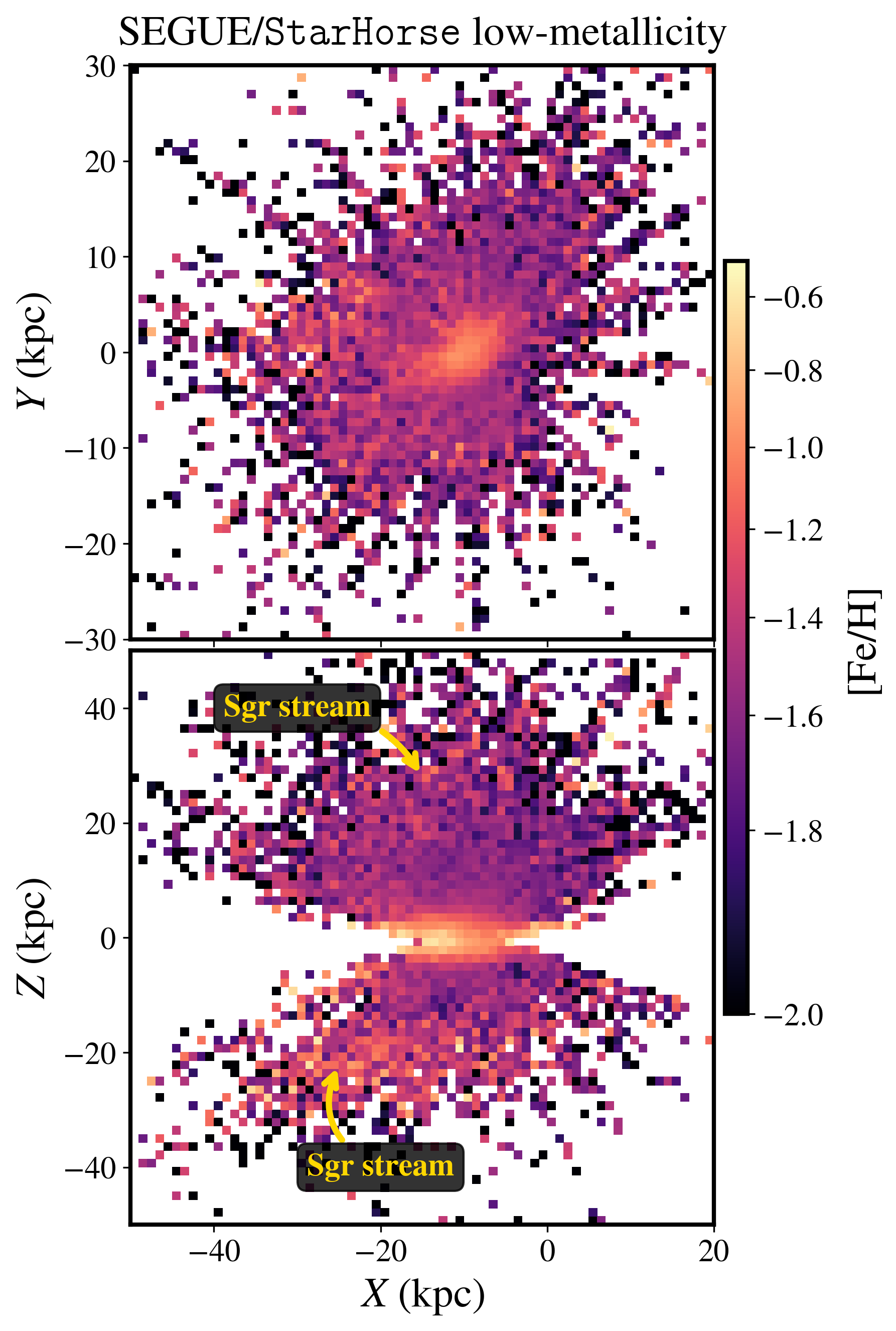
Figure 1: Cartesian Galactocentric projections of the SEGUE/StarHorse low-metallicity sample. Top: $(X,Y)$. Bottom: $(X,Z)$. Spatial bins are color-coded by their mean [Fe/H] values. The attentive reader may notice the footprint of Sgr stream as metal-rich trails at ${|Z|}\gtrsim 20\,{\rm kpc}$.

We applied StarHorse to this SEGUE$+$Gaia EDR3 sample in order to estimate precise distances that would allow us to study the Sgr stream; at ${\geq}10\,{\rm kpc}$ from the Sun, our derived uncertainties are at the level of ${\sim}13\%$. The medians of the derived posterior distributions are adopted as our nominal values, while $16$th and $84$th percentiles are taken as uncertainties. Further details regarding stellar-evolution models and geometric priors can be found in Queiroz et al. (2018, 2020) and Anders et al. (2019). See also Anders et al. (2022) for details regarding the compiled photometric data.

With the StarHorse output at hand, we restrict our sample to stars with moderate ($<$20%) fractional Gaussian uncertainties in their estimated distance values. We refer to this catalog as the “SEGUE/StarHorse low-metallicity sample” or close variations of that. We refer the interested reader to Perottoni et al. (2022) for an initial application of these data. Its coverage in a Cartesian Galactocentric projection can be appreciated in Figure 1. By color-coding this plot with the mean [Fe/H] in spatial bins, the footprint of Sgr stream is already perceptible as metal-rich trails at ${|Z|}\gtrsim 20\,{\rm kpc}$.

2.2 Kinematics and Dynamics

Positions ($\alpha$, $\delta$) and proper motions ($\mu_{\alpha}^{*}=\mu_{\alpha}\cos{\delta}$, $\mu_{\delta}$) on the sky, $v_{\rm los}$ values from SEGUE, and StarHorse heliocentric distances are converted to Galactocentric Cartesian phase-space coordinates using Astropy Python tools (Astropy Collaboration et al., 2013, 2018). The adopted position of the Sun with respect to the Galactic center is $(X,Y,Z)_{\odot}=(-8.2,0.0,0.0208)\,{\rm kpc}$ (Bland-Hawthorn & Gerhard, 2016; Bennett & Bovy, 2019). The local circular velocity is $\mathbf{V_{\rm circ}}=(0.0,232.8,0.0)\,{\rm km\,s^{-1}}$ (McMillan, 2017), while the Sun’s peculiar motion with respect to $\mathbf{V_{\rm circ}}$ is $(U,V,W)_{\odot}=(11.10,12.24,7.25)\,{\rm km\ s^{-1}}$ (Schönrich et al., 2010).

For reference, we write, below, how each component of the total angular momentum ($\boldsymbol{L}$) is calculated.

$$L_{x}=YV_{z}-ZV_{y}$$ (1)

$$L_{y}=ZV_{x}-XV_{z}$$

$$L_{z}=XV_{y}-YV_{x}{,}$$

where $L=\sqrt{L_{x}^{2}+L_{y}^{2}+L_{z}^{2}}$. We recall that, although $\boldsymbol{L}$ is not fully conserved in an axisymmetric potential, with the exception of the $L_{z}$ component, it has been historically used for the identification of substructure in the Galaxy as it preserves reasonable amount of clumping over time (see Helmi 2020 for a review)

For the entire SEGUE/StarHorse low-metallicity sample, we also compute other dynamical parameters, such as orbital energy ($E$) and actions ($\boldsymbol{J}=(J_{R},J_{\phi},J_{z})$ in cylindrical frame). The azimuthal action is equivalent to the vertical component of angular momentum ($J_{\phi}\equiv L_{z}$) and we use these nomenclatures interchangeably. In order to obtain these quantities, orbits are integrated for 10 Gyr forward with the AGAMA package (Vasiliev, 2019) within the axisymmetric Galactic model of McMillan (2017). A total of 100 initial conditions were generated for each star with a Monte Carlo approach, accounting for uncertainties in proper motions, $v_{\rm los}$, and distance. The final orbital parameters are taken as the medians of the resulting distributions, with $16$th and $84$th percentiles as uncertainties.

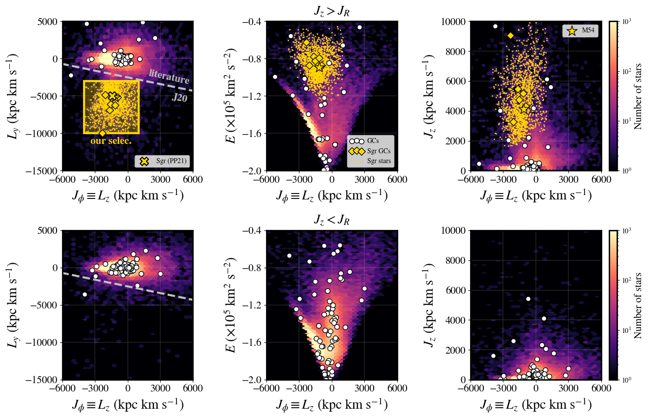
Figure 2: Upper row: $J_{z}>J_{R}$ (predominantly polar orbits). Bottom: $J_{z}<J_{R}$ (radial/eccentric orbits). Background density maps are produced with the full SEGUE/StarHorse low-metallicity sample. White dots are Galactic GCs. Those associated with Sgr dSph/stream are displayed as yellow diamonds, with M54 as the star symbol (see text). Left panels: $(L_{z},L_{y})$. Our Sgr stream selection is shown as the yellow box. The gray dashed line exhibits the J20 criterion. The yellow cross is the central location of Sgr in this space according to PP21. Yellow dots represent Sgr stream members. Middle: $(L_{z},E)$. Right: $(L_{z},J_{z})$.

3 Sgr Stream in SEGUE

3.1 Selection of Members

Given our goals, we seek to construct a sample of Sgr stream members that is both ($i$) larger in size and ($ii$) with greater purity than previously considered by J20, but ($iii$) with a similarly extended metallicity range, reaching the extremely metal-poor ($\rm[Fe/H]<-3$) regime. J20 have shown that stars from the Sgr stream can be selected to exquisite completeness in the ($L_{z},L_{y}$) plane, which exploits the polar nature of their orbits. We reproduce their criterion in Figure 2 (left panels, dashed lines). However, PP21 have recently argued that the J20’s criterion also includes ${\approx}21\%$ of interlopers.

We inspect the aforementioned ($L_{z},L_{y}$) plane, splitting it into $J_{z}>J_{R}$ (predominantly polar orbits; Figure 2, top row) and $J_{z}<J_{R}$ (radial/eccentric orbits; bottom row) as was done in Naidu et al. (2020). In Figure 2, there exists an excess of stars toward negative values of $L_{y}$ (top left panel), which is prograde (top middle), and with $J_{z}\gtrsim 2000\,{\rm kpc\,km\,s^{-1}}$ (top right; Thomas & Battaglia, 2022), corresponding to the footprint of Sgr stream (see Malhan et al., 2022). In the case where $J_{z}<J_{R}$, where Sgr stream completely vanishes, the ($L_{z},E$) space is dominated by the Gaia Sausage/Enceladus (GSE; Belokurov et al., 2018; Haywood et al., 2018, also Helmi et al. 2018).

Developing on the above-described facts, we quantify how useful the $J_{z}>J_{R}$ condition is for eliminating potential GSE contaminants within our Sgr stream members. We look at a suite of chemodynamical simulations of Milky Way-mass galaxies with stellar halos produced by a single GSE-like merger presented in Amarante et al. (2022). Within these models, the fraction of GSE debris that end up (at redshift $z=0$) on orbits with $J_{z}>J_{R}$ is always below 9%. Therefore, we incorporated this condition to our selection as it should remove ${>}90\%$ of potential GSE stars.

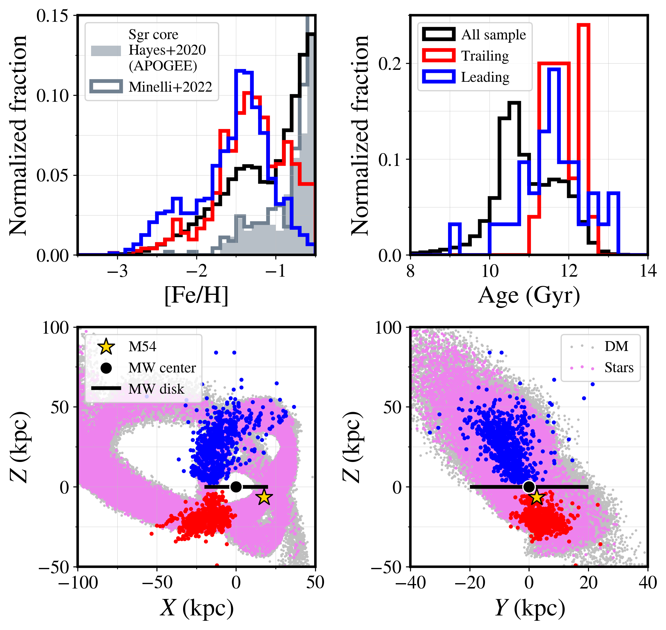
Figure 3: Top row: metallicity (left) and age (right) distributions. In both panels, blue and red histograms represent the leading and trailing arms of Sgr stream, respectively. Filled and empty grayish histograms show the $\rm[Fe/H]$ distributions of Sgr’s core according to Hayes et al. (2020, updated to APOGEE DR17) and Minelli et al. (2022), respectively. The complete SEGUE/StarHorse low-metallicity sample is shown in black. Bottom row: configuration space in the Galactic Cartesian coordinate system. Left: $(X,Z)$. Right: $(Y,Z)$. Blue and red dots are stars associated with the leading and trailing arms, respectively. The location of the M54 GC, which coincides with the center of Sgr dSph, is shown as the yellow star symbol. The background Sgr model (stream$+$surviving core) is from V21, where gray and pink dots are dark matter and stellar particles, respectively. The Milky Way’s center and disk (40 kpc diameter) are illustrated by the black circle and line, respectively.

Lastly, we restrict the kinematic locus occupied by Sgr stream in ($L_{z},L_{y}$) in comparison to J20 and consider only those stars at ${>}6$ kpc from the Sun, in conformity with the V21 model. In this work, the conditions that a star must fulfill in order to be considered a genuine member of Sgr stream are listed below:

• $J_{z}>J_{R}$;

• ${\rm heliocentric\ distance}>6\,{\rm kpc}$;

• $-10<L_{y}/(10^{3}\,{\rm kpc}\,{\rm km}\,{\rm s}^{-1})<-3$;

• $-4<L_{z}/(10^{3}\,{\rm kpc}\,{\rm km}\,{\rm s}^{-1})<+1$.

This selection is delineated by the yellow box in the top left panel of Figure 2. It is clear that our criteria is more conservative than J20’s. Nevertheless, the raw size of our final Sgr stream sample (${\sim}1600$ stars) is twice as large as the one presented by these authors despite the sharp cut at $\rm[Fe/H]<-0.5$. Moreover, the metallicity range covered reaches $\rm[Fe/H]\sim-3$, with ${\gtrsim}200$ VMP stars in the sample (top left in Figure 3). Finally, although these Sgr stream candidates were identified from their locus in ($L_{z},L_{y}$), we found them to be spatially cohesive and in agreement with the V21 model in configuration space (bottom row of Figure 3). Even so, the potential contamination by other known polar streams (see Malhan et al., 2021) is explored in Appendix A.

With this new set of selection criteria at hand, we verified which known Galactic globular clusters (GCs) would be connected to the Sgr system. Consequently, we examined the orbital properties of 170 GCs from the Gaia EDR3-based catalog of Vasiliev & Baumgardt (2021). We found that a total of seven GCs can be linked to this group, including NGC 6715/M54, Whiting1, Koposov1, Terzan7, Arp2, Terzan8, and Pal12. We note that M54 has long been recognized to be the nuclear star cluster of Sgr dSph (e.g., Bellazzini et al., 2008). Furthermore, most of these other GCs had already been attributed to Sgr by several authors (Massari et al., 2019; Bellazzini et al., 2020; Forbes, 2020; Kruijssen et al., 2020; Callingham et al., 2022; Malhan et al., 2022).

3.2 Leading and Trailing Arms

We begin our study of Sgr stream’s stellar populations by looking at the metallicity distributions obtained for the leading and trailing arms and differences between them. In Figure 3, the immediately perceptible feature is the excess of VMP stars in the leading arm. On the contrary, the trailing arm presents a significant contribution of metal-rich ($\rm[Fe/H]\gtrsim-1$) stars. This property had already been noticed by several authors (e.g., Carlin et al., 2018; Hayes et al., 2020) and is recovered despite the intentional bias of the SEGUE catalog to low-metallicity stars (note the excess at $\rm[Fe/H]\lesssim-1$ in the black/all-sample histogram; see Bonifacio et al. 2021 and Whitten et al. 2021 for discussions).

The final median [Fe/H] values we obtained for the leading and trailing arms are $-1.46^{+0.02}_{-0.03}$ and $-1.28^{+0.03}_{-0.05}$, respectively, where upper and lower limits represent bootstrapped ($10^{4}$ times) 95% confidence intervals. These metallicity values derived from SEGUE are $\sim$0.3–0.4 dex lower than the ones obtained from APOGEE data (Hayes et al., 2020; Limberg et al., 2022), but we recall that this is due to SEGUE’s target selection function (Rockosi et al., 2022).

We further notice that the location of these metallicity peaks for both arms of the stream are well aligned with the secondary, more metal-poor, $\rm[Fe/H]$ peak for stars in the core of Sgr (grayish histograms in Figure 3; Hayes et al. 2020/APOGEE and Minelli et al. 2022). Although differences in metallicity scales might be at play, this observation could be relevant for the evolution of the Sgr system in the presence of the Milky Way and LMC.

From StarHorse’s output, we should also, in principle, be able to access information regarding ages for individual stars as this parameter is a byproduct of the isochrone-fitting procedure (e.g., Edvardsson et al. 1993, Jørgensen & Lindegren 2005, and Sanders & Das 2018). However, there are some caveats in this approach. First, it becomes increasingly difficult to distinguish between isochrones of different ages toward both the cooler regions of the main sequence as well as the upper portions of the red giant branch (see figure 2 of Souza et al. 2020 for a didactic visualization). However, it is still possible to go around this issue by looking at the turnoff and subgiant areas where isochrones tend to be better segregated (see discussion in Vickers et al., 2021). Second, even at these evolutionary stages, variations in ages and metallicities have similar effects on the color–magnitude diagram (e.g., Yi et al. 2001, Demarque et al. 2004, Pietrinferni et al. 2004, 2006, and Dotter et al. 2008). Hence, spectroscopic [Fe/H] values can be leveraged as informative priors to break this age–metallicity degeneracy. Third, distant non-giant stars are quite faint, which is the case for our Sgr stream sample. This is where SEGUE’s exquisite depth, with targets as faint as $g=19.5$, where $g$ is SDSS broad band centered at $4800$ Å (Fukugita et al., 1996), comes in handy.

In this spirit, we attempt to provide a first estimate of the typical ages for stars in Sgr stream. Similar to recent efforts (Bonaca et al., 2020; Buder et al., 2022; Xiang & Rix, 2022), we selected stars in the SEGUE/StarHorse low-metallicity sample near the turnoff and subgiant stages. For the sake of consistency, for this task, we utilized stellar parameters derived by StarHorse itself during the isochrone-fitting process as these will be directly correlated with the ages at hand. These turnoff and subgiant stars are mostly contained within $4.5<\log g_{\rm SH}\lesssim 3.6$ and $T_{\rm eff,SH}\gtrsim 5250\,{\rm K}$, where the subscript “SH” indicates values from StarHorse instead of SSPP. A parallel paper describes in detail this (sub)sample with reliable ages (Queiroz et al., submitted). In any case, for the purpose of this work, we highlight that typical differences between SEGUE’s atmospheric parameters and those obtained with StarHorse are at the level of SSPP’s internal precision.

We found a total of 56 turnoff or subgiant stars in Sgr stream (31 in the leading arm plus 25 in the trailing one) for which ages are most reliable (top right panel of Figure 3). As expected, these are quite faint ($17.5<g<19.5$), which reinforces the value of a deep spectroscopic survey such as SEGUE. Members of Sgr stream (blue and red histograms representing leading and trailing arms, respectively) appear to be older (11–12 Gyr) than the bulk of our sample, which is mostly composed of thick-disk stars. It is reassuring that the age distribution for the entire SEGUE/StarHorse low-metallicity sample (black) peaks at 10–11 Gyr, which is, indeed, in agreement with ages derived from asteroseismic data for the chemically-defined, i.e., high-$\alpha$, thick-disk population (Silva Aguirre et al., 2018; Miglio et al., 2021). We quantify this visual interpretation with a kinematically-selected thick-disk sample, following $100<|\mathbf{V}-\mathbf{V_{\rm circ}|/({\rm km\,s^{-1}}})<180$ (check Venn et al., 2004; Bensby et al., 2014; Li & Zhao, 2017; Posti et al., 2018; Koppelman et al., 2020), where $\mathbf{V}=(V_{x},V_{y},V_{z})$ is the total velocity vector of a given star, i.e., $V=\sqrt{V_{x}^{2}+V_{y}^{2}+V_{z}^{2}}$. Within the SEGUE/StarHorse low-metallicity data (${\sim}7,800$ stars), we found a median age of 10.6 Gyr for this population.

For Sgr stream specifically, the bootstrapped median age for the leading arm is $11.6^{+0.4}_{-0.2}\,{\rm Gyr}$. For the trailing arm, we found $11.8^{+0.3}_{-0.2}\,{\rm Gyr}$. This translates to $11.7^{+0.3}_{-0.2}\,{\rm Gyr}$ considering all Sgr stream stars. Of course, uncertainties for individual stars are still substantial, usually at the level of ${>}25\%$ (${\sim}3$ Gyr). Therefore, we hope that it will be possible to test this scenario, that the Sgr stream is dominated by stars older (by ${\sim}1$ Gyr) than those from the Galactic thick disk, with data provided by the upcoming generation of spectroscopic surveys, such as 4MOST (de Jong et al., 2019), SDSS-V (Kollmeier et al., 2017), and WEAVE (Dalton et al., 2016), and building on the statistical isochrone-fitting framework of StarHorse.

3.3 Evolution of Velocity Dispersion with Metallicity

The original motivation for us to identify Sgr stream members in the SEGUE/StarHorse catalog was to analyze the evolution of its kinematics extending deeply into the VMP regime, similar to Gibbons et al. (2017) and J20. The former was the first to propose the existence of two populations in Sgr stream. Its main limitation was the lack of complete phase-space information, which are now available thanks to Gaia. Regarding the latter, the caveats were the small amount of (${\sim}50$) VMP stars in their sample (from H3 survey) and potential contamination by Milky Way foreground stars ( PP21, ). Here, instead of splitting Sgr stream into two components, our approach is to model its velocity distribution across different [Fe/H] intervals. The results of this exercise can provide constraints to future chemodynamical simulations attempting to reproduce the Sgr system as was recently done for GSE (Amarante et al., 2022).

Figure 4 displays the distributions of total velocity ($V$) across different metallicity ranges, from VMP (left) to metal-rich (right). The color scheme is blue/red for leading/trailing arm as in Figure 3. From visual inspection, one can notice that both histograms become broader at lower [Fe/H] values. In order to quantify this effect of increasing velocity dispersion ($\sigma_{V}$) with decreasing [Fe/H], we model these distributions, while also accounting for uncertainties, using a Markov chain Monte Carlo (MCMC) method implemented with the emcee Python package (Foreman-Mackey et al., 2013). As in Li et al. (2017, 2018), the Gaussian $\log$-likelihood function is written as

$$\log{\mathcal{L}}=-\dfrac{1}{2}\sum_{i=1}^{N}\left[\log{\left(\sigma^{2}_{V}+\sigma^{2}_{V,i}\right)}+\dfrac{\left(V_{i}-\langle V\rangle\right)^{2}}{\left(\sigma^{2}_{V}+\sigma^{2}_{V,i}\right)}\right]{,}$$ (2)

where $V_{i}$ and $\sigma_{V,i}$ are the total velocity and its respective uncertainty for the $i$th star within a given [Fe/H] bin. We adopt only the following uniform priors: $0<\langle V\rangle/({\rm km}\,{\rm s}^{-1})<500$ and $\sigma_{V}>0$. Lastly, we run the MCMC sampler for 500 steps with 50 walkers, including a burn-in stage of 100. Although some of the $V$ histograms in Figure 4 show non-Gaussian tails, this exercise is sufficient for the present purpose.

The results of our MCMC calculations are presented in Table 1. Upper and lower limits are 16th and 84th percentiles, respectively, from the posterior distributions. Between $-1.5<\rm[Fe/H]\leq-0.5$, we found no statistically-significant (${<}1\sigma$) evidence for $\sigma_{V}$ variations. However, at $\rm[Fe/H]\leq-1.5$, the $\sigma_{V}$ increases substantially for both arms. According to present data, the VMP component of Sgr stream (left panel of Figure 4) is dynamically hotter than its metal-rich counterpart at the ${\gtrsim}2\sigma$ level. We also verified that this effect is less prominent (${\sim}1\sigma$) for GSE (green histograms in Figure 4; Table 1) even with a not-so-pure (at least 18% contamination; Limberg et al. 2022) selection (Feuillet et al., 2020), which is to be expected given the advanced stage of phase-mixing of this substructure.

Figure 4: Distributions of $V=\sqrt{V_{x}^{2}+V_{y}^{2}+V_{z}^{2}}$ in intervals of [Fe/H]. From left to right, we move from the VMP to the metal-rich regime. Blue, red, and green histograms represent the leading arm, trailing arm, and GSE, respectively.

Table 1: Velocity Dispersion for the Leading and Trailing Arms of Sgr, as well as GSE, in bins of [Fe/H]

Substructure	$\sigma_{V}$	$\sigma_{V}$	$\sigma_{V}$	$\sigma_{V}$
	(km s-1)	(km s-1)	(km s-1)	(km s-1)
	$\rm[Fe/H]\leq-2.0$	$-2.0<\rm[Fe/H]\leq-1.5$	$-1.5<\rm[Fe/H]\leq-1.0$	$-1.0<\rm[Fe/H]\leq-0.5$
Leading	$70^{+4}_{-4}\%$   (194)	$62^{+3}_{-3}\%$   (284)	$51^{+2}_{-2}\%$   (405)	$53^{+5}_{-4}\%$    (94)
Trailing	$44^{+6}_{-5}\%$    (62)	$38^{+3}_{-3}\%$   (185)	$32^{+2}_{-5}\%$   (319)	$28^{+2}_{-2}\%$   (203)
GSE	$87^{+2}_{-2}\%$ (1153)	$86^{+1}_{-1}\%$ (4314)	$83^{+1}_{-1}\%$ (8020)	$82^{+2}_{-2}\%$ (1322)

Now, we put our results in context with those in the literature. With the understanding that Sgr stream is comprised of two kinematically distinct populations (J20), the increasing $\sigma_{V}$ as a function of decreasing metallicity can be interpreted as larger fractions of the “diffuse” ( J20, ) component contributing to the low-[Fe/H] (dynamically hotter) bins. On the contrary, the “main” component, which contains most of the stars of the substructure, is preferentially associated with the high-[Fe/H] (dynamically colder) intervals.

PP21 recently argued that the broad velocity distribution for metal-poor stars in Sgr stream could be an artifact of Milky Way contamination in the J20 Sgr stream data. However, this effect is still clearly present in our $2{\times}$ larger sample with more rigorous selection criteria. To summarize, in the low-metallicity regime, there appears to be considerable contribution from both ancient and recently formed wraps of the stream. On the other hand, at high metallicities ($\rm[Fe/H]>-1.0$), only the newest wrap is represented.

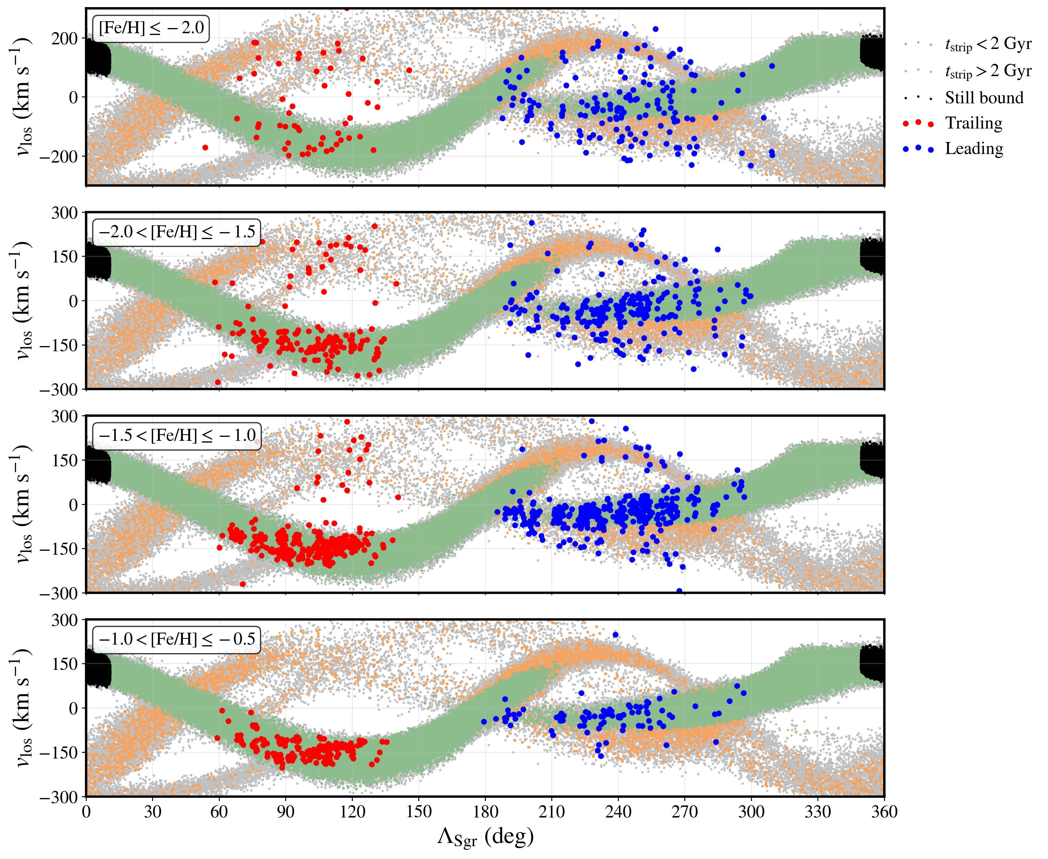
Figure 5: Sgr stream in $(\Lambda_{\rm Sgr},v_{\rm los})$ space. As in Figure 3, blue and red dots are stars associated with the leading and trailing arms, respectively. Dark matter and stellar particles from the V21 model are shown as gray and colored dots, respectively. Green dots are attributed to the new ($t_{\rm strip}<2\,{\rm Gyr}$) and orange ones to the old ($t_{\rm strip}>2\,{\rm Gyr}$) wraps. Black dots remain bound to the progenitor until the present day (redshift $z=0$), i.e., the end of the simulation. From top to bottom, we move from the VMP to the metal-rich regime following the same [Fe/H] ranges of Figure 4 and Table 1.

4 Model Comparisons

In this section, we interpret the phase-space properties of Sgr stream and how they correlate with chemistry via the comparison of our Sgr sample with the V21 model.

4.1 Model Properties, Assumptions, and Limitations

V21’s is a tailored $N$-body model of the Sgr system designed to match several properties of its tidal tails. In particular, in order to mimic the aforementioned misalignment between the stream track and its proper motions in the leading arm, the authors invoke the presence an LMC with a total mass of $1.5\times 10^{11}\,M_{\odot}$, compatible with Erkal et al. (2019), Shipp et al. (2021), and Koposov et al. (2022). The initial conditions are set to reproduce the present-day positions and velocities of both Sgr and LMC building on earlier results (Vasiliev & Belokurov, 2020). However, unlike the LMC and Sgr, the Milky Way is not modeled in a live $N$-body scheme. Hence, it comes with the limitation that V21 depend on the Chandrasekhar analytical prescription for dynamical friction (e.g., Mo et al., 2010). See Ramos et al. (2022) for a discussion on how this approximation might influence the stripping history of the stream.

In the fiducial model, the initial stellar mass of Sgr dSph is $2\times 10^{8}\,M_{\odot}$ and follows a spherical King density profile (King, 1962). Moreover, the system is embedded in an, also spherical, extended dark matter halo of $3.6\times 10^{9}\,M_{\odot}$. Other key features of V21’s work is the capability of recovering crucial kinematic and structural features of Sgr’s remnant (as in Vasiliev & Belokurov, 2020), accounting for perturbations introduced by the gravitational field of LMC (Garavito-Camargo et al., 2019, 2021; Cunningham et al., 2020; Petersen & Peñarrubia, 2020, 2021; Erkal et al., 2021), and properly following mass loss suffered by the system.

Despite the close match between observations and the V21 model, there are a few limitations that could affect their results. For instance, the model does not account for the gaseous component , which may be relevant for the distribution of the debris as discussed in Wang et al. (2022) and references therein. An additional caveat is the lack of bifurcations in the modeled stream, as originally observed by Belokurov et al. (2006) and Koposov et al. (2012, see discussions by ). Finally, Sgr likely experienced at least one pericentric passage $\gtrsim$6 Gyr ago as can be inferred from dynamical perturbations in the Galactic disk (Binney & Schönrich, 2018; Laporte et al., 2018, 2019; Bland-Hawthorn & Tepper-García, 2021; McMillan et al., 2022, and see Antoja et al. 2018) as well as the star-formation histories of both the Milky Way (Ruiz-Lara et al., 2020) and Sgr itself (Siegel et al., 2007; de Boer et al., 2015). Hence, the V21 simulation, which starts only 3 Gyr in the past, is unable to cover this earlier interaction.

4.2 New and Old Wraps

Figure 5 shows observational and simulation data in $(\Lambda_{\rm Sgr},v_{\rm los})$, where $\Lambda_{\rm Sgr}$ is the stream longitude coordinate as defined by Majewski et al. (2003) based on Sgr’s orbital plane. Leading/trailing arm stars are blue/red dots. These are overlaid to the V21 model, where gray and colored points are dark matter and stellar particles, respectively. We split these simulated particles according to their stripping time ($t_{\rm strip}$). For the remainder of this paper, we refer to the portion of the (simulated) stream formed more recently ($t_{\rm strip}<2\,{\rm Gyr}$) as the “new” wrap (green). The more ancient ($t_{\rm strip}>2\,{\rm Gyr}$) component is henceforth the “old” wrap (orange). Stellar particles that are still bound to the progenitor by the end of the simulation (redshift $z=0$) are colored black.

We divide our Sgr stream data in the same metallicity intervals as Figure 4/Table 1. Essentially, our selected members of Sgr stream share all regions of phase space with the V21 model particles. Notwithstanding, the bottom-most panel of Figure 5 reveals a first interesting feature. Metal-rich stars in the sample are almost exclusively associated with the new wrap, though this is more difficult to immediately assert for the leading arm because of the overlap between new and old portions within $180\degree\lesssim\Lambda_{\rm Sgr}<300\degree$.

As we move toward lower-metallicity (upper) panels of Figure 5, we see larger fractions of observed Sgr stream stars coinciding with the old wrap in phase space. At the same time, the dense groups of stars overlapping with the new wrap fade away as we reach the VMP regime (top panel). As a direct consequence, stream members are more spread along the $v_{\rm los}$ axis in Figure 5, which, then, translates into the higher $\sigma_{V}$ discussed in Section 3.3 for metal-poor/VMP stars. In general, the new wrap is preferentially associated with metal-rich stars, but also extends into the VMP realm. Conversely, the old component contains exclusively metal-poor ($\rm[Fe/H]\lesssim-1$) stars. Therefore, these suggest that, at low metallicities, Sgr stream is composed of a mixture between old and new wraps and this phenomenon drives the increasing $\sigma_{V}$ quantified in Table 1.

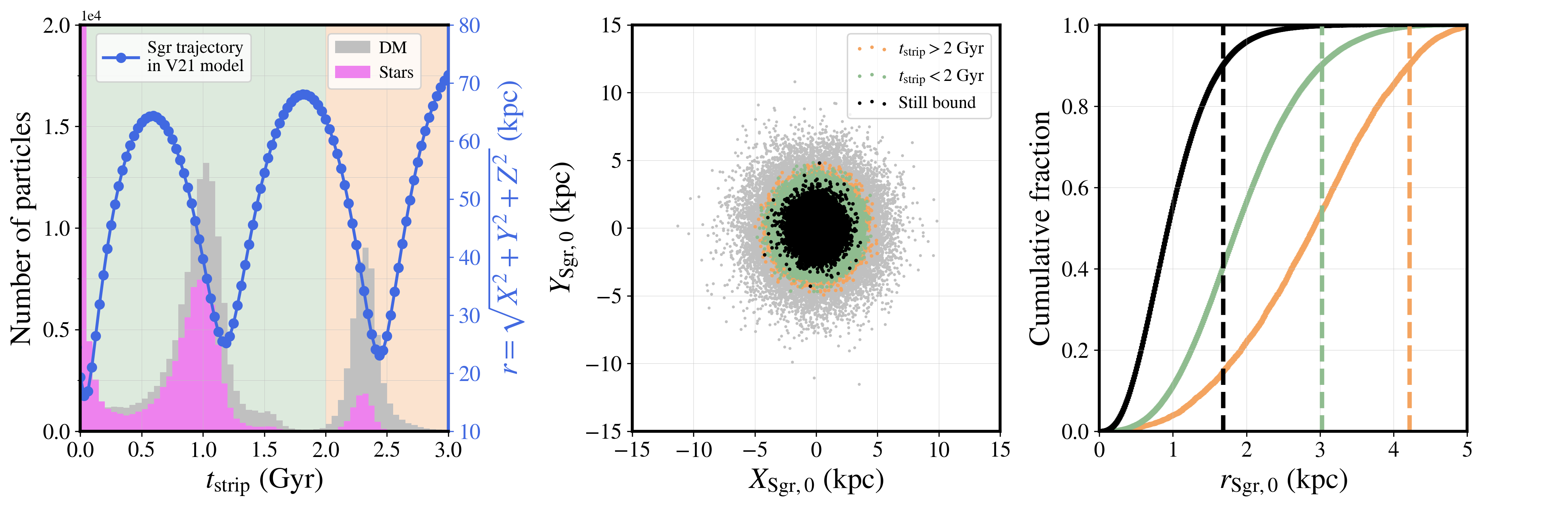
Figure 6: Left: distributions of $t_{\rm strip}$ for dark matter (gray) and stellar (pink) particles in the V21 model of Sgr (stream$+$dSph) system. The orbital trajectory of Sgr in the form of Galactocentric distance is presented as the overlapping blue line and circles. Middle: dark matter and stellar (colored dots) particles in configuration space, where $(X,Y)_{\rm Sgr,0}$ are spatial coordinates in a Sgr-centered sytem in the initial snapshot of the same V21 model (see text). Right: cumulative distribution functions of galactocentric radii ($r_{\rm Sgr,0}$) of the same model particles, also centered around Sgr in the initial snapshot. Vertical dashed lines mark the positions containing 90% of the stars of each component. In all panels, the color scheme is the same as Figure 5, where orange represents stars that end up as the old wrap of the stream ($t_{\rm strip}>2$ Gyr), green is for the new wrap ($t_{\rm strip}<2$ Gyr), and black are those particles that remain bound to Sgr dSph until present-day/end of the simulation ($t_{\rm strip}=0$).

4.3 Sgr dSph Before its Disruption

The dichotomy between metal-rich/cold and metal-poor/hot portions of Sgr stream has been suggested, by J20, to be linked to the existence of a stellar halo-like structure in Sgr dSph prior to its infall. This stellar halo would have larger velocity dispersion, be spatially more extended, and have lower metallicity than the rest of the Sgr galaxy. As a consequence of its kinematics, this component would be stripped at earlier times. Indeed, we verified that the old wrap of Sgr stream, stripped ${>}2\,{\rm Gyr}$ ago in V21’s model, is mainly associated with metal-poor stars (Figure 5), in conformity with J20’s hypothesis. Meanwhile, the majority of the most metal-rich stars can be attributed to the new wrap. In order to check how the present-day properties of Sgr stream are connected to those of its dSph progenitor, hence testing other conjectures of J20, we now look at the initial snapshot of V21’s simulation, including the satellite’s orbit and disruption history.

Simply to comprehend the assembly of the stream over time according to the V21 model, we plot the distribution of $t_{\rm strip}$ in the left panel of Figure 6. The excess at $t_{\rm strip}=0$ is due to $N$-body particles that remain bound to the progenitor. On top of these histograms, we add the trajectory of Sgr dSph in the simulation (blue line and dots) in terms of its Galactocentric distance. With this visualization, it is clear how intense episodes of material being stripped (at both $2.0<t_{\rm strip}/{\rm Gyr}\lesssim 2.7$ and $0.5\lesssim t_{\rm strip}/{\rm Gyr}\lesssim 1.5$) are intrinsically related to close encounters between Sgr and the Milky Way (at ${\sim}2.5$ and ${\sim}1.2$ Gyr ago), which originates the new and old wraps discussed in Section 4.2. Also, note how most of the material is associated with the recently formed component (new wrap) of the stream.

In order to test J20’s conjecture that the stripped portion of Sgr dSph associated with the formation of the old wrap was already dynamically hotter than the new one prior to the galaxy’s disruption, we check the $\sigma_{V}$, with respect to Sgr, of these components in the initial snapshot of V21’s simulation, which starts 3 Gyr in the past (redshift $z\sim 0.25$ in Planck Collaboration et al. 2020 cosmology). Indeed, the $\sigma_{V}$ of stars that end up forming the old wrap, i.e., stripped at earlier times, is higher (${\sim}18$ km s^-1) in comparison to the $\sigma_{V}$ of stars from the new component (${\sim}14$ km s^-1).

In the middle panel of Figure 6, the initial snapshot is presented in configuration space as $(X,Y)_{\rm Sgr,0}$, a Sgr-centered frame. The orange dots ($t_{\rm strip}>2$ Gyr/old wrap) in this plot are less centrally concentrated (90% of stellar particles within $\sim$4 kpc) than the green ones ($t_{\rm strip}<2$ Gyr/new wrap; 90% within 3 kpc). This behavior is clear from the right panel of the same figure that shows the cumulative distributions of galactocentric radii ($r_{\rm Sgr,0}$) in the same system. Also, stars that remain bound until redshift $z=0$ have even lower $\sigma_{V}$ (${\sim}11$ km s^-1) and are spatially more concentrated (90% within ${<}2$ kpc) than the other components.

From the above-described properties of the V21 model, we can infer that the periphery of the simulated Sgr dSph contains a larger fraction of stars that end up as the old wrap (stripped earlier) in comparison to its central regions. Therefore, with the understanding that the old wrap is essentially composed of low-metallicity stars), we reach the conclusion that the core regions of Sgr dSph were more metal-rich than its outskirts prior to its accretion. We recall that, indeed, previous works reported evidence for a metallicity gradient in the Sgr remnant (Bellazzini et al., 1999; Layden & Sarajedini, 2000; Siegel et al., 2007; McDonald et al., 2013; Mucciarelli et al., 2017; Vitali et al., 2022). Nevertheless, fully understanding how these stellar-population variations in the Sgr system relate to its interaction with the Milky Way remains to be seem (for example, via induced star-formation bursts; Hasselquist et al. 2021).

Although our interpretation favors a scenario where Sgr dSph had enough time to develop a metallicity gradient before its disruption, quantifying this effect is difficult. One way to approach this would be painting the model with ad hoc metallicity gradients and, then, comparing with, for instance, the present-day [Fe/H] variations observed across the Sgr stream (Hayes et al. 2020 and references therein). We defer this exploration to a forthcoming paper.

5 Chemical Abundances

5.1 $\alpha$ Elements

Apart from $T_{\rm eff}$, $\log g$, and $\rm[Fe/H]$, the SSPP also estimates $\alpha$-element abundances based on the wavelength range of $4500\leq\lambda/{\rm\textup{\AA}}\leq 5500$ (Lee et al., 2011), which contains several Ti I and Ti II lines as well as the Mg I triplet (${\sim}5200$ Å). de Boer et al. (2014) utilized $[\alpha/{\rm Fe}]$ values made available by SEGUE for stars in Sgr stream to argue that a “knee” existed at $\rm[Fe/H]\lesssim-1.3$ in the [$\alpha$/Fe]–[Fe/H] diagram (Wallerstein, 1962; Tinsley, 1979) for this substructure. However, this result is not supported by contemporaneous high-resolution spectroscopic data, specially from APOGEE (Hayes et al., 2020; Horta et al., 2022; Limberg et al., 2022), also H3 (Johnson et al., 2020; Naidu et al., 2020). If the position of Sgr’s $\alpha$ knee was truly located at such high [Fe/H], it would imply that it should be even more massive than GSE under standard chemical-evolution prescriptions (e.g., Matteucci & Brocato, 1990).

Here, we revisit the $\alpha$ abundances for Sgr stream using SEGUE, but with a larger sample with lower contamination. In the left panel of Figure 7, we see the continuous decrease of [$\alpha$/Fe] as a function of increasing metallicity for both the Sgr stream and GSE. Most important, at a given value of [Fe/H], the median [$\alpha$/Fe] of Sgr stream (both leading and trailing arms) is lower than GSE’s. This difference becomes more prominent at $\rm[Fe/H]\gtrsim-1.5$, in agreement with the aforementioned high-resolution spectroscopy results from both H3 and APOGEE. Despite that, the low accuracy/precision of [$\alpha$/Fe] in SEGUE still makes it difficult to attribute stars to certain populations on an individual basis.

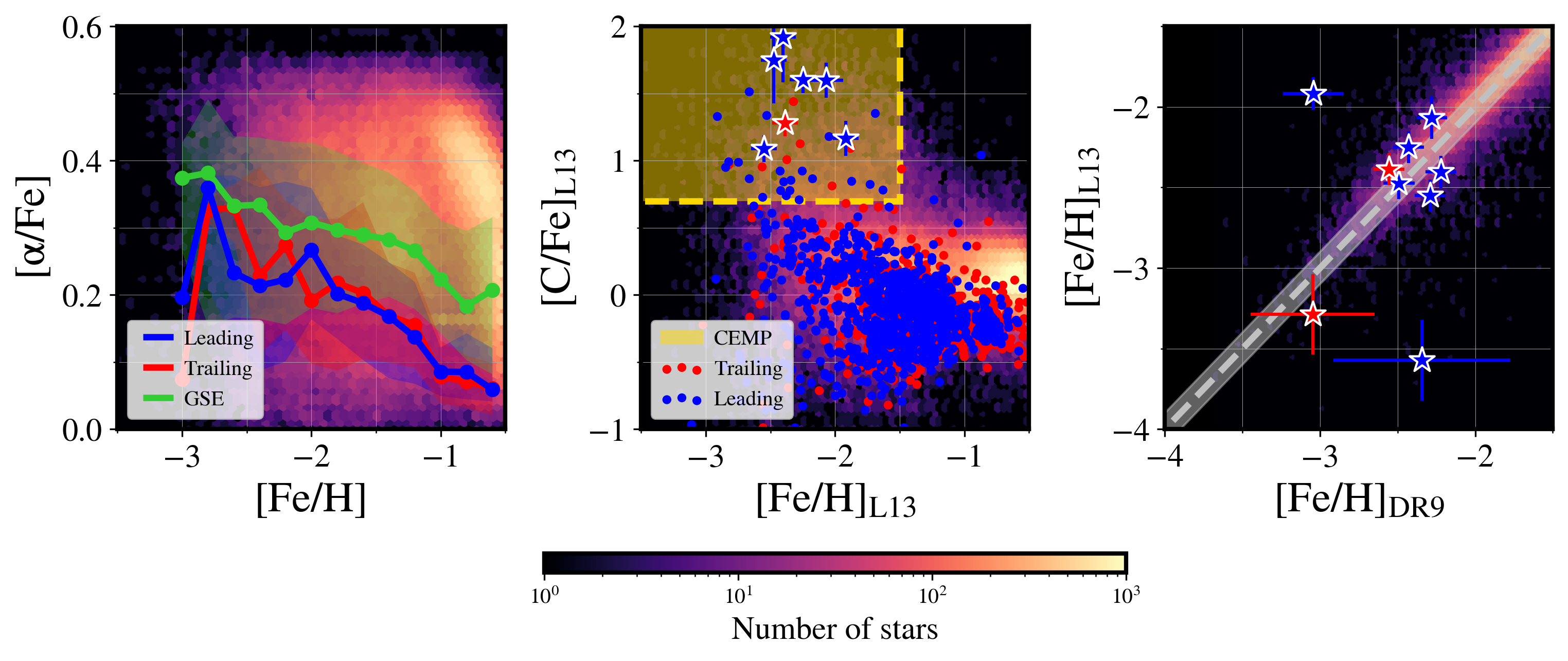
Figure 7: Left: [$\alpha$/Fe]–[Fe/H]. Green line is the running median of GSE’s [$\alpha$/Fe] values in bins of 0.2 dex in [Fe/H], with the shaded area covering 16th and 84th percentiles. Blue and red lines and shaded regions are the same, but for the leading and trailing arms of Sgr stream, respectively. Middle: [C/Fe]–[Fe/H]. The yellow rectangle marks the locus of CEMP stars. Blue/red symbols are leading/trailing arm stars. Candidate ($3\sigma$; see text) CEMP stars are shown as star symbols. Right: $\rm[Fe/H]_{\rm L13}$–$\rm[Fe/H]_{\rm DR9}$, where the “L13”and “DR9” subscripts refer to [Fe/H] values either from Lee et al. (2013) or SEGUE’s standard catalog from SDSS DR9. Background density maps represent the full SEGUE/StarHorse low-metallicity sample.

5.2 Carbon

With the SEGUE low-metallicity data at hand, we also explore carbon abundances. In particular, we are interested in finding carbon-enhanced metal-poor (CEMP; $\rm[C/Fe]>+0.7$ and $\rm[Fe/H]<-1$; see Beers & Christlieb 2005, Aoki et al. 2007, and Placco et al. 2014) stars in Sgr stream. The reasoning for that being the recent results by Chiti et al. (2020, also and ) where these authors found no CEMP star in their sample of Sgr dSph members within $-3.1<\rm[Fe/H]\lesssim-1.5$. Moreover, we utilize observations of Sgr stream as a shortcut to check for potential differences in CEMP fractions between a dwarf galaxy and the Milky Way’s stellar halo (see Venn et al., 2012; Kirby et al., 2015; Salvadori et al., 2015; Chiti et al., 2018) in a homogeneous setting. Given that the CEMP phenomenon, specially at $\rm[Fe/H]\lesssim-2.5$, is connected to nucleosynthesis events associated with the first generations of stars, perhaps Population III (e.g., Nomoto et al., 2013; Yoon et al., 2016; Chiaki et al., 2017), identifying such objects provide clues about the first chemical-enrichment processes that happened in a galaxy.

Throughout this section, we consider carbon abundances obtained for SEGUE spectra by Lee et al. (2013, see also , , and ). Inconveniently, this catalog also comes with slight variations of the stellar atmospheric parameters in comparison with the public SEGUE DR9 release. Therefore, in order to confidently identify CEMP stars, we first select candidates using only Lee et al. (2013) [C/Fe] and [Fe/H] (subscripts “L13” in Figure 7). Then, we compare $\rm[Fe/H]_{\rm L13}$ with [Fe/H] values from our standard DR9 sample ($\rm[Fe/H]_{\rm DR9}$; right panel of Figure 7) to confirm their low-metallicity nature.

The middle panel of Figure 7 ([C/Fe]–[Fe/H]) exhibits our selection of CEMP candidates (yellow box). Note that we take only those stars at $\rm[Fe/H]_{\rm L13}<-1.5$, for consistency with the metallicity range covered by Chiti et al. (2020). Expanding this boundary to $\rm[Fe/H]_{\rm L13}<-1$ would only include a couple of additional CEMP candidates. We discovered a total of 39 likely-CEMP stars (33 at $\rm[Fe/H]_{\rm L13}<-2$). With this sample at hand, we looked for those candidates confidently ($3\sigma$ in $\rm[C/Fe]_{\rm L13}$) encompassed by the CEMP criteria. We found 7 such objects, shown as star symbols in Figure 7. Although two of these CEMP stars have discrepant metallicity determinations ($\rm[Fe/H]_{\rm L13}$ vs. $\rm[Fe/H]_{\rm DR9}$; right panel of Figure 7), we can still confidently assert that there exist CEMP stars in Sgr stream.

A possible explanation for the lack of CEMP stars in Chiti et al.’s (2020) sample could be their photometric target selection, which was based on SkyMapper DR1 (Wolf et al., 2018). The excess of carbon, hence the exquisite strength of the CH $G$-band, is capable of depressing the continuum extending to the wavelength region of the Ca II K/H lines, close to the center of SkyMapper’s $v$ filter ($3825\textup{\AA}$; see Da Costa et al. 2019 and references therein), a phenomenon referred to as “carbon veiling” (Yoon et al., 2020). A scenario where, if confirmed, the surviving core of Sgr dSph has a lower CEMP fraction than its outskirts/stream at a given metallicity could be similar to what potentially happens to the Milky Way’s bulge and halo (Arentsen et al., 2021). Either way, the unbiased discovery of additional VMP stars in Sgr as well as other dSph satellites (e.g., Skúladóttir et al., 2021) will be paramount for us to advance our understanding about the earliest stages of chemical enrichment in these systems.

Finally, we also calculate the fraction of CEMP stars in Sgr stream and compare it with the Milky Way. Arentsen et al. (2022) has recently demonstrated that various observational efforts focused on the discovery and analysis of metal-poor stars via low/medium-resolution (up to $\mathcal{R}\sim 3000$) spectroscopy report inconsistent CEMP fractions among them (Lee et al., 2013; Placco et al., 2018, 2019; Aguado et al., 2019; Arentsen et al., 2020; Yuan et al., 2020b; Limberg et al., 2021a; Shank et al., 2022). However, we reinforce that it is not our goal to provide absolute CEMP fractions (e.g., Rossi et al., 2005; Lucatello et al., 2006; Yoon et al., 2018), but rather use the SEGUE/StarHorse low-metallicity sample to make a homogeneous comparison. For this reason, we do not perform any evolutionary corrections (as in Placco et al. 2014) to the carbon abundances of Lee et al. (2013). The overall fraction of CEMP stars in the whole sample at $\rm[Fe/H]<-2$, but excluding Sgr, is $19\pm 1\%$ within the same $\log g$ range. For the whole Sgr stream, leading and trailing arms altogether, this number is $16\pm 5\%$. Limiting our analysis to only giants ($T_{\rm eff}<5800$ K and $\log g<4$), we find 12% for both the stream and full sample. Therefore, we conclude the SEGUE carbon-abundance data does not provide evidence for variations in the CEMP frequency between Sgr (stream) and the Milky Way.

6 Conclusions

In this work, we performed a chemodynamical study of Sgr stream, the tidal tails produced by the ongoing disruption of Sgr dSph galaxy. Because of recent literature results, we were particularly interested in exploring the VMP regime of this substructure. Our main goals were to quantify the kinematic properties of this population as well as search for CEMP stars. For the task, we leveraged low-resolution spectroscopic and astrometric data from SEGUE DR9 and Gaia EDR3, respectively. Moreover, this catalog was combined with broad-band photometry from various sources in order to deliver precise distances for ${\sim}175,000$ low-metallicity ($\rm[Fe/H]\leq-0.5$) stars via Bayesian isochrone-fitting in a new StarHorse run (Figure 1), an effort that is fully described in an accompanying paper (Queiroz et al., submitted). Our main conclusions can be summarized as follows.

• We delineated a new set of selection criteria for the Sgr stream based on angular momenta and actions (Figure 2). Despite being more conservative than previous works (e.g., J20 and Naidu et al. 2020), we identify ${\sim}1600$ members of Sgr stream, which is twice as many as these authors. Out of these, there are ${>}200$ VMP stars as well as 7 GCs.

• Reassuringly, although the SEGUE target selection inflates the number of metal-poor stars ($\rm[Fe/H]<-1$; Figure 3), we found the leading arm to be more metal-poor, by ${\sim}0.2$ dex, than the trailing one. This is in agreement with many previous works (notably Hayes et al., 2020).

• We provided the first age estimates for individual stars in Sgr stream. For the task, we constructed a subsample of 56 turnoff/subgiant stars in this substructure, for which StarHorse ages are most reliable. We found an overall median age of $11.7^{+0.3}_{-0.2}\,{\rm Gyr}$, which is ${\sim}1$ Gyr older than the bulk of thick-disk stars according both to our own SEGUE/StarHorse data as well as asteroseismic estimates (Miglio et al., 2021).

• We found ($2\sigma$) evidence for increasing velocity dispersion in Sgr stream between its metal-rich and VMP populations (Figure 4/Table 1). Similar findings were presented by J20, but were contested by PP21. Now, we reassert the former’s findings with a $2{\times}$ larger sample and more rigorously-selected Sgr stream members (Figure 4/Table 1).

• With the $N$-body model of V21, we found that the new wrap (composed of stars recently stripped; $t_{\rm strip}<2\,{\rm Gyr}$) of Sgr stream preferentially contains metal-rich ($\rm[Fe/H]>-1.0$) stars. Conversely, the old wrap ($t_{\rm strip}>2\,{\rm Gyr}$) is exclusively associated with metal-poor stars ($\rm[Fe/H]<-1.0$) in phase space. Hence, the increasing velocity dispersion with decreasing [Fe/H] is driven by the mixture between these components, i.e., larger fractions of the old wrap are found at lower metallicities, while the metal-rich population is only representative of the new wrap (Figure 5).

• Looking at the initial snapshot of the V21 simulation, we found that stars that end up forming the old wrap are dynamically hotter and less centrally concentrated than those that compose the new wrap. With the understanding that the old wrap contains stars of lower metallicities, this implies that the outskirts of Sgr dSph, prior to disruption, were more metal-poor than is core regions, i.e., internal [Fe/H] variations in the galaxy.

• On the chemical-abundance front, SEGUE data allowed us to verify that the [$\alpha$/Fe] of Sgr stream decreases with increasing [Fe/H]. Most important, at a given metallicity, we ascertained that the median [$\alpha$/Fe] of Sgr stream is lower than GSE’s, in conformity with other recent efforts (Hasselquist et al., 2021; Horta et al., 2022; Limberg et al., 2022).

• We confidently (${>}3\sigma$) identify CEMP stars in Sgr stream. Also, its CEMP fraction is compatible ($1\sigma$) with the overall SEGUE catalog. Hence, we argue that the apparent lack of CEMP stars in Sgr dSph (Chiti et al., 2020, and references therein) could be associated with target-selection effects and/or small sample sizes.

This paper emphasizes how powerful the synergy between deep spectroscopy and astrometric data can be in our quest to unravel the outer Galactic halo. It also shows how crucial the fully Bayesian approach of StarHorse is for the task of deriving precise parameters (mainly distances) even for faint stars. In fact, the SEGUE/StarHorse catalog provides a glimpse of the scientific potential that will be unlocked by the next generation of wide-field surveys such as 4MOST, SDSS-V, and WEAVE. Finally, we reinforce the importance of tailored $N$-body models as fundamental tools for interpreting of the complex debris left behind by disrupted dwarf galaxies in the Milky Way’s halo.

Appendix A Other Dwarf-galaxy Polar Streams

In order to test if our Sgr stream selection is robust against the presence of other known dwarf-galaxy polar stellar streams (see Malhan et al., 2021), we assembled literature data for Cetus (Yuan et al., 2019, originally found by Newberg et al. 2009), Orphan (Koposov et al., 2019, first described by Belokurov et al. 2006, 2007), LMS-1/Wukong (Yuan et al., 2020a, also Naidu et al. 2020), and Helmi streams (O’Hare et al., 2020, discovered by Helmi et al. 1999). In this process, we made an effort to compile only members of streams found with automatic algorithms (Myeong et al., 2018a, b; Yuan et al., 2018). The only exception is Orphan, whose members were selected based on the stream’s track on the sky as well as proper motions. Note that, originally, Yuan et al. (2020a) dubbed the LMS-1/Wukong substructure as “low-mass stellar-debris stream”, hence the acronym. Almost at the same time, Naidu et al. (2020) identified a very similar dynamical group of stars in $(L_{z},E)$ with the H3 survey and referred to it as “Wukong”. For now, we keep both nomenclatures, similar to what several authors adopt for GSE. Apart from the $J_{z}>J_{R}$ condition, we followed Naidu et al. (2022) and Limberg et al. (2021b, which builds on , , and ) to apply further constraints to both Orphan and Helmi streams, respectively, in order to guarantee better purity for these samples.

The kinematic/dynamical locus occupied by the polar streams is shown in Figure 8. Crucially, they do not overlap the box in $(L_{z},L_{y})$ defined for Sgr (yellow region in the left panel). However, note how the J20 criteria actually encompasses the bulk of Orphan stream stars, which emphasizes the importance of our more rigorous selection. Helmi stream stars are the ones that reach the closest to our Sgr boundary in angular-momentum space. Although no stars from this substructure actually fulfill our entire set of selection criteria for Sgr, it is difficult to assert that Helmi stream interlopers are nonexistent in our Sgr sample. One way to quantify the cross-contamination between halo substructures would be to explore $N$-body models, similar to what has been recently done by Sharpe et al. (2022). For the time being, even without such a dedicated effort, we highlight that our criteria achieves several benchmarks, such as eliminating ${>}90\%$ of potential GSE stars, removing low-$J_{z}$ contaminants from the Galactic disk(s), and excluding most stars from other well-known dwarf-galaxy streams.

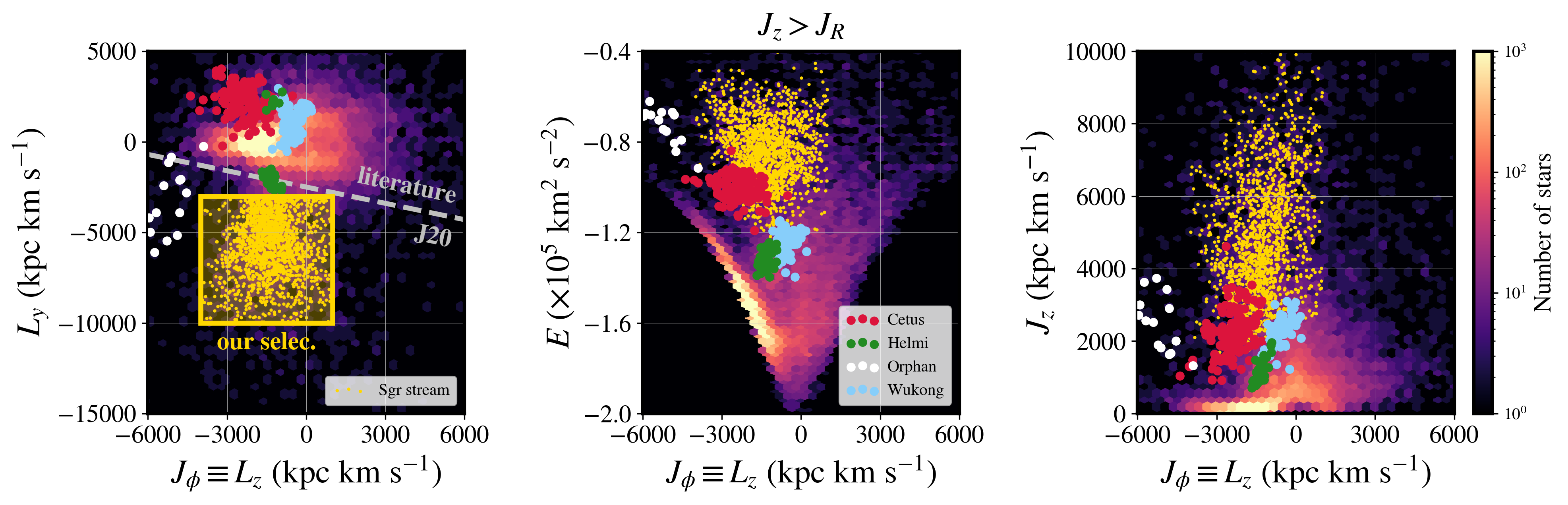
Figure 8: Similar to the top row of Figure 2 ($J_{z}>J_{R}$), but including literature data for dwarf-galaxy polar streams. Left: $(L_{z},L_{y})$. The dashed line shows the J20 criterion for selecting Sgr members. The yellow box exhibits our criteria. Colored dots represent stars from Sgr (yellow), Cetus (red), Orphan (white), LMS-1/Wukong (blue), and Helmi (green) streams (see text). Middle: $(L_{z},E)$. Right: $(L_{z},J_{z})$ In all panels, density maps represent the full SEGUE/StarHorse low-metallicity sample.

References

- Abdurro’uf et al. (2022) Abdurro’uf, Accetta, K., Aerts, C., et al. 2022, ApJS, 259, 35, doi: 10.3847/1538-4365/ac4414
- Aguado et al. (2019) Aguado, D. S., Youakim, K., González Hernández, J. I., et al. 2019, MNRAS, 490, 2241, doi: 10.1093/mnras/stz2643
- Aguado et al. (2021) Aguado, D. S., Myeong, G. C., Belokurov, V., et al. 2021, MNRAS, 500, 889, doi: 10.1093/mnras/staa3250
- Ahn et al. (2012) Ahn, C. P., Alexandroff, R., Allende Prieto, C., et al. 2012, ApJS, 203, 21, doi: 10.1088/0067-0049/203/2/21
- Alard (1996) Alard, C. 1996, ApJ, 458, L17, doi: 10.1086/309917
- Allende Prieto et al. (2008) Allende Prieto, C., Sivarani, T., Beers, T. C., et al. 2008, AJ, 136, 2070, doi: 10.1088/0004-6256/136/5/2070
- Amarante et al. (2022) Amarante, J. A. S., Debattista, V. P., Beraldo E Silva, L., Laporte, C. F. P., & Deg, N. 2022, ApJ, 937, 12, doi: 10.3847/1538-4357/ac8b0d
- Anders et al. (2019) Anders, F., Khalatyan, A., Chiappini, C., et al. 2019, A&A, 628, A94, doi: 10.1051/0004-6361/201935765
- Anders et al. (2022) Anders, F., Khalatyan, A., Queiroz, A. B. A., et al. 2022, A&A, 658, A91, doi: 10.1051/0004-6361/202142369
- Antoja et al. (2020) Antoja, T., Ramos, P., Mateu, C., et al. 2020, A&A, 635, L3, doi: 10.1051/0004-6361/201937145
- Antoja et al. (2018) Antoja, T., Helmi, A., Romero-Gómez, M., et al. 2018, Nature, 561, 360, doi: 10.1038/s41586-018-0510-7
- Aoki et al. (2007) Aoki, W., Beers, T. C., Christlieb, N., et al. 2007, ApJ, 655, 492, doi: 10.1086/509817
- Arentsen et al. (2022) Arentsen, A., Placco, V. M., Lee, Y. S., et al. 2022, arXiv e-prints, arXiv:2206.04081. https://arxiv.org/abs/2206.04081
- Arentsen et al. (2020) Arentsen, A., Starkenburg, E., Martin, N. F., et al. 2020, MNRAS, 496, 4964, doi: 10.1093/mnras/staa1661
- Arentsen et al. (2021) Arentsen, A., Starkenburg, E., Aguado, D. S., et al. 2021, MNRAS, 505, 1239, doi: 10.1093/mnras/stab1343
- Astropy Collaboration et al. (2013) Astropy Collaboration, Robitaille, T. P., Tollerud, E. J., et al. 2013, A&A, 558, A33, doi: 10.1051/0004-6361/201322068
- Astropy Collaboration et al. (2018) Astropy Collaboration, Price-Whelan, A. M., Sipőcz, B. M., et al. 2018, AJ, 156, 123, doi: 10.3847/1538-3881/aabc4f
- Beers & Christlieb (2005) Beers, T. C., & Christlieb, N. 2005, ARA&A, 43, 531, doi: 10.1146/annurev.astro.42.053102.134057
- Bellazzini et al. (1999) Bellazzini, M., Ferraro, F. R., & Buonanno, R. 1999, MNRAS, 304, 633, doi: 10.1046/j.1365-8711.1999.02377.x
- Bellazzini et al. (2020) Bellazzini, M., Ibata, R., Malhan, K., et al. 2020, A&A, 636, A107, doi: 10.1051/0004-6361/202037621
- Bellazzini et al. (2006) Bellazzini, M., Newberg, H. J., Correnti, M., Ferraro, F. R., & Monaco, L. 2006, A&A, 457, L21, doi: 10.1051/0004-6361:20066002
- Bellazzini et al. (2008) Bellazzini, M., Ibata, R. A., Chapman, S. C., et al. 2008, AJ, 136, 1147, doi: 10.1088/0004-6256/136/3/1147
- Belokurov et al. (2018) Belokurov, V., Erkal, D., Evans, N. W., Koposov, S. E., & Deason, A. J. 2018, MNRAS, 478, 611, doi: 10.1093/mnras/sty982
- Belokurov et al. (2006) Belokurov, V., Zucker, D. B., Evans, N. W., et al. 2006, ApJ, 642, L137, doi: 10.1086/504797
- Belokurov et al. (2007) Belokurov, V., Evans, N. W., Irwin, M. J., et al. 2007, ApJ, 658, 337, doi: 10.1086/511302
- Belokurov et al. (2014) Belokurov, V., Koposov, S. E., Evans, N. W., et al. 2014, MNRAS, 437, 116, doi: 10.1093/mnras/stt1862
- Bennett & Bovy (2019) Bennett, M., & Bovy, J. 2019, MNRAS, 482, 1417, doi: 10.1093/mnras/sty2813
- Bensby et al. (2014) Bensby, T., Feltzing, S., & Oey, M. S. 2014, A&A, 562, A71, doi: 10.1051/0004-6361/201322631
- Binney & Schönrich (2018) Binney, J., & Schönrich, R. 2018, MNRAS, 481, 1501, doi: 10.1093/mnras/sty2378
- Bland-Hawthorn & Gerhard (2016) Bland-Hawthorn, J., & Gerhard, O. 2016, ARA&A, 54, 529, doi: 10.1146/annurev-astro-081915-023441
- Bland-Hawthorn & Tepper-García (2021) Bland-Hawthorn, J., & Tepper-García, T. 2021, MNRAS, 504, 3168, doi: 10.1093/mnras/stab704
- Bonaca et al. (2020) Bonaca, A., Conroy, C., Cargile, P. A., et al. 2020, ApJ, 897, L18, doi: 10.3847/2041-8213/ab9caa
- Bonifacio et al. (2021) Bonifacio, P., Monaco, L., Salvadori, S., et al. 2021, A&A, 651, A79, doi: 10.1051/0004-6361/202140816
- Buder et al. (2022) Buder, S., Lind, K., Ness, M. K., et al. 2022, MNRAS, 510, 2407, doi: 10.1093/mnras/stab3504
- Bullock & Johnston (2005) Bullock, J. S., & Johnston, K. V. 2005, ApJ, 635, 931, doi: 10.1086/497422
- Callingham et al. (2022) Callingham, T. M., Cautun, M., Deason, A. J., et al. 2022, MNRAS, 513, 4107, doi: 10.1093/mnras/stac1145
- Cargile et al. (2020) Cargile, P. A., Conroy, C., Johnson, B. D., et al. 2020, ApJ, 900, 28, doi: 10.3847/1538-4357/aba43b
- Carlin et al. (2018) Carlin, J. L., Sheffield, A. A., Cunha, K., & Smith, V. V. 2018, ApJ, 859, L10, doi: 10.3847/2041-8213/aac3d8
- Carollo et al. (2012) Carollo, D., Beers, T. C., Bovy, J., et al. 2012, ApJ, 744, 195, doi: 10.1088/0004-637X/744/2/195
- Chandra et al. (2022) Chandra, V., Naidu, R. P., Conroy, C., et al. 2022, arXiv e-prints, arXiv:2212.00806. https://arxiv.org/abs/2212.00806
- Chiaki et al. (2017) Chiaki, G., Tominaga, N., & Nozawa, T. 2017, MNRAS, 472, L115, doi: 10.1093/mnrasl/slx163
- Chiti & Frebel (2019) Chiti, A., & Frebel, A. 2019, ApJ, 875, 112, doi: 10.3847/1538-4357/ab0f9f
- Chiti et al. (2020) Chiti, A., Hansen, K. Y., & Frebel, A. 2020, ApJ, 901, 164, doi: 10.3847/1538-4357/abb1ae
- Chiti et al. (2018) Chiti, A., Simon, J. D., Frebel, A., et al. 2018, ApJ, 856, 142, doi: 10.3847/1538-4357/aab663
- Chou et al. (2010) Chou, M.-Y., Cunha, K., Majewski, S. R., et al. 2010, ApJ, 708, 1290, doi: 10.1088/0004-637X/708/2/1290
- Chou et al. (2007) Chou, M.-Y., Majewski, S. R., Cunha, K., et al. 2007, ApJ, 670, 346, doi: 10.1086/522483
- Conroy et al. (2019) Conroy, C., Bonaca, A., Cargile, P., et al. 2019, ApJ, 883, 107, doi: 10.3847/1538-4357/ab38b8
- Cooper et al. (2013) Cooper, A. P., D’Souza, R., Kauffmann, G., et al. 2013, MNRAS, 434, 3348, doi: 10.1093/mnras/stt1245
- Cooper et al. (2010) Cooper, A. P., Cole, S., Frenk, C. S., et al. 2010, MNRAS, 406, 744, doi: 10.1111/j.1365-2966.2010.16740.x
- Coronado et al. (2018) Coronado, J., Rix, H.-W., & Trick, W. H. 2018, MNRAS, 481, 2970, doi: 10.1093/mnras/sty2468
- Crnojević et al. (2016) Crnojević, D., Sand, D. J., Spekkens, K., et al. 2016, ApJ, 823, 19, doi: 10.3847/0004-637X/823/1/19
- Cunningham et al. (2020) Cunningham, E. C., Garavito-Camargo, N., Deason, A. J., et al. 2020, ApJ, 898, 4, doi: 10.3847/1538-4357/ab9b88
- Da Costa et al. (2019) Da Costa, G. S., Bessell, M. S., Mackey, A. D., et al. 2019, MNRAS, 489, 5900, doi: 10.1093/mnras/stz2550
- Dalton et al. (2016) Dalton, G., Trager, S., Abrams, D. C., et al. 2016, in Society of Photo-Optical Instrumentation Engineers (SPIE) Conference Series, Vol. 9908, Ground-based and Airborne Instrumentation for Astronomy VI, ed. C. J. Evans, L. Simard, & H. Takami, 99081G, doi: 10.1117/12.2231078
- de Boer et al. (2014) de Boer, T. J. L., Belokurov, V., Beers, T. C., & Lee, Y. S. 2014, MNRAS, 443, 658, doi: 10.1093/mnras/stu1176
- de Boer et al. (2015) de Boer, T. J. L., Belokurov, V., & Koposov, S. 2015, MNRAS, 451, 3489, doi: 10.1093/mnras/stv946
- de Jong et al. (2019) de Jong, R. S., Agertz, O., Berbel, A. A., et al. 2019, The Messenger, 175, 3, doi: 10.18727/0722-6691/5117
- Demarque et al. (2004) Demarque, P., Woo, J.-H., Kim, Y.-C., & Yi, S. K. 2004, ApJS, 155, 667, doi: 10.1086/424966
- Dotter et al. (2008) Dotter, A., Chaboyer, B., Jevremović, D., et al. 2008, ApJS, 178, 89, doi: 10.1086/589654
- Edvardsson et al. (1993) Edvardsson, B., Andersen, J., Gustafsson, B., et al. 1993, A&A, 275, 101
- Erkal et al. (2019) Erkal, D., Belokurov, V., Laporte, C. F. P., et al. 2019, MNRAS, 487, 2685, doi: 10.1093/mnras/stz1371
- Erkal et al. (2021) Erkal, D., Deason, A. J., Belokurov, V., et al. 2021, MNRAS, 506, 2677, doi: 10.1093/mnras/stab1828
- Fabricius et al. (2021) Fabricius, C., Luri, X., Arenou, F., et al. 2021, A&A, 649, A5, doi: 10.1051/0004-6361/202039834
- Fellhauer et al. (2006) Fellhauer, M., Belokurov, V., Evans, N. W., et al. 2006, ApJ, 651, 167, doi: 10.1086/507128
- Feuillet et al. (2020) Feuillet, D. K., Feltzing, S., Sahlholdt, C. L., & Casagrande, L. 2020, MNRAS, 497, 109, doi: 10.1093/mnras/staa1888
- Forbes (2020) Forbes, D. A. 2020, MNRAS, 493, 847, doi: 10.1093/mnras/staa245
- Foreman-Mackey (2016) Foreman-Mackey, D. 2016, JOSS, 1, 24, doi: 10.21105/joss.00024
- Foreman-Mackey et al. (2013) Foreman-Mackey, D., Hogg, D. W., Lang, D., & Goodman, J. 2013, PASP, 125, 306, doi: 10.1086/670067
- Fukugita et al. (1996) Fukugita, M., Ichikawa, T., Gunn, J. E., et al. 1996, AJ, 111, 1748, doi: 10.1086/117915
- Gaia Collaboration et al. (2016a) Gaia Collaboration, Prusti, T., de Bruijne, J. H. J., et al. 2016a, A&A, 595, A1, doi: 10.1051/0004-6361/201629272
- Gaia Collaboration et al. (2016b) Gaia Collaboration, Brown, A. G. A., Vallenari, A., et al. 2016b, A&A, 595, A2, doi: 10.1051/0004-6361/201629512
- Gaia Collaboration et al. (2018) —. 2018, A&A, 616, A1, doi: 10.1051/0004-6361/201833051
- Gaia Collaboration et al. (2021) —. 2021, A&A, 649, A1, doi: 10.1051/0004-6361/202039657
- Garavito-Camargo et al. (2019) Garavito-Camargo, N., Besla, G., Laporte, C. F. P., et al. 2019, ApJ, 884, 51, doi: 10.3847/1538-4357/ab32eb
- Garavito-Camargo et al. (2021) —. 2021, ApJ, 919, 109, doi: 10.3847/1538-4357/ac0b44
- Gibbons et al. (2017) Gibbons, S. L. J., Belokurov, V., & Evans, N. W. 2017, MNRAS, 464, 794, doi: 10.1093/mnras/stw2328
- Hansen et al. (2018) Hansen, C. J., El-Souri, M., Monaco, L., et al. 2018, ApJ, 855, 83, doi: 10.3847/1538-4357/aa978f
- Hasselquist et al. (2021) Hasselquist, S., Hayes, C. R., Lian, J., et al. 2021, ApJ, 923, 172, doi: 10.3847/1538-4357/ac25f9
- Hayes et al. (2020) Hayes, C. R., Majewski, S. R., Hasselquist, S., et al. 2020, ApJ, 889, 63, doi: 10.3847/1538-4357/ab62ad
- Haywood et al. (2018) Haywood, M., Di Matteo, P., Lehnert, M. D., et al. 2018, ApJ, 863, 113, doi: 10.3847/1538-4357/aad235
- Helmi (2004) Helmi, A. 2004, ApJ, 610, L97, doi: 10.1086/423340
- Helmi (2020) —. 2020, ARA&A, 58, 205, doi: 10.1146/annurev-astro-032620-021917
- Helmi et al. (2018) Helmi, A., Babusiaux, C., Koppelman, H. H., et al. 2018, Nature, 563, 85, doi: 10.1038/s41586-018-0625-x
- Helmi & White (1999) Helmi, A., & White, S. D. M. 1999, MNRAS, 307, 495, doi: 10.1046/j.1365-8711.1999.02616.x
- Helmi & White (2001) —. 2001, MNRAS, 323, 529, doi: 10.1046/j.1365-8711.2001.04238.x
- Helmi et al. (1999) Helmi, A., White, S. D. M., de Zeeuw, P. T., & Zhao, H. 1999, Nature, 402, 53, doi: 10.1038/46980
- Hernitschek et al. (2017) Hernitschek, N., Sesar, B., Rix, H.-W., et al. 2017, ApJ, 850, 96, doi: 10.3847/1538-4357/aa960c
- Hogg et al. (2019) Hogg, D. W., Eilers, A.-C., & Rix, H.-W. 2019, AJ, 158, 147, doi: 10.3847/1538-3881/ab398c
- Horta et al. (2022) Horta, D., Schiavon, R. P., Mackereth, J. T., et al. 2022, arXiv e-prints, arXiv:2204.04233. https://arxiv.org/abs/2204.04233
- Hunter (2007) Hunter, J. D. 2007, Computing in Science and Engineering, 9, 90, doi: 10.1109/MCSE.2007.55
- Hyde et al. (2015) Hyde, E. A., Keller, S., Zucker, D. B., et al. 2015, ApJ, 805, 189, doi: 10.1088/0004-637X/805/2/189
- Ibata et al. (2020) Ibata, R., Bellazzini, M., Thomas, G., et al. 2020, ApJ, 891, L19, doi: 10.3847/2041-8213/ab77c7
- Ibata et al. (2001a) Ibata, R., Irwin, M., Lewis, G., Ferguson, A. M. N., & Tanvir, N. 2001a, Nature, 412, 49. https://arxiv.org/abs/astro-ph/0107090
- Ibata et al. (2001b) Ibata, R., Irwin, M., Lewis, G. F., & Stolte, A. 2001b, ApJ, 547, L133, doi: 10.1086/318894
- Ibata et al. (1994) Ibata, R. A., Gilmore, G., & Irwin, M. J. 1994, Nature, 370, 194, doi: 10.1038/370194a0
- Ibata et al. (1995) —. 1995, MNRAS, 277, 781, doi: 10.1093/mnras/277.3.781
- Johnson et al. (2020) Johnson, B. D., Conroy, C., Naidu, R. P., et al. 2020, ApJ, 900, 103, doi: 10.3847/1538-4357/abab08
- Johnston (1998) Johnston, K. V. 1998, ApJ, 495, 297, doi: 10.1086/305273
- Johnston et al. (2005) Johnston, K. V., Law, D. R., & Majewski, S. R. 2005, ApJ, 619, 800, doi: 10.1086/426777
- Jørgensen & Lindegren (2005) Jørgensen, B. R., & Lindegren, L. 2005, A&A, 436, 127, doi: 10.1051/0004-6361:20042185
- Kauffmann et al. (1993) Kauffmann, G., White, S. D. M., & Guiderdoni, B. 1993, MNRAS, 264, 201, doi: 10.1093/mnras/264.1.201
- Keller et al. (2010) Keller, S. C., Yong, D., & Da Costa, G. S. 2010, ApJ, 720, 940, doi: 10.1088/0004-637X/720/1/940
- Kim et al. (2022) Kim, C., Lee, Y. S., Beers, T. C., & Masseron, T. 2022, JKAS, 55, 23, doi: 10.5303/JKAS.2022.55.2.23
- King (1962) King, I. 1962, AJ, 67, 471, doi: 10.1086/108756
- Kirby et al. (2015) Kirby, E. N., Guo, M., Zhang, A. J., et al. 2015, ApJ, 801, 125, doi: 10.1088/0004-637X/801/2/125
- Kluyver et al. (2016) Kluyver, T., Ragan-Kelley, B., Pérez, F., et al. 2016, in Positioning and Power in Academic Publishing: Players, Agents and Agendas, ed. F. Loizides & B. Schmidt (Amsterdam: IOS Press), 87
- Kollmeier et al. (2017) Kollmeier, J. A., Zasowski, G., Rix, H.-W., et al. 2017, arXiv e-prints, arXiv:1711.03234. https://arxiv.org/abs/1711.03234
- Koo et al. (2022) Koo, J.-R., Lee, Y. S., Park, H.-J., Kim, Y. K., & Beers, T. C. 2022, ApJ, 925, 35, doi: 10.3847/1538-4357/ac3423
- Koposov et al. (2010) Koposov, S. E., Rix, H.-W., & Hogg, D. W. 2010, ApJ, 712, 260, doi: 10.1088/0004-637X/712/1/260
- Koposov et al. (2012) Koposov, S. E., Belokurov, V., Evans, N. W., et al. 2012, ApJ, 750, 80, doi: 10.1088/0004-637X/750/1/80
- Koposov et al. (2019) Koposov, S. E., Belokurov, V., Li, T. S., et al. 2019, MNRAS, 485, 4726, doi: 10.1093/mnras/stz457
- Koposov et al. (2022) Koposov, S. E., Erkal, D., Li, T. S., et al. 2022, arXiv e-prints, arXiv:2211.04495. https://arxiv.org/abs/2211.04495
- Koppelman et al. (2020) Koppelman, H. H., Hagen, J. H. J., & Helmi, A. 2020, arXiv e-prints, arXiv:2009.04849. https://arxiv.org/abs/2009.04849
- Koppelman et al. (2019) Koppelman, H. H., Helmi, A., Massari, D., Roelenga, S., & Bastian, U. 2019, A&A, 625, A5, doi: 10.1051/0004-6361/201834769
- Kruijssen et al. (2020) Kruijssen, J. M. D., Pfeffer, J. L., Chevance, M., et al. 2020, MNRAS, 498, 2472, doi: 10.1093/mnras/staa2452
- Laporte et al. (2018) Laporte, C. F. P., Johnston, K. V., Gómez, F. A., Garavito-Camargo, N., & Besla, G. 2018, MNRAS, 481, 286, doi: 10.1093/mnras/sty1574
- Laporte et al. (2019) Laporte, C. F. P., Minchev, I., Johnston, K. V., & Gómez, F. A. 2019, MNRAS, 485, 3134, doi: 10.1093/mnras/stz583
- Law et al. (2005) Law, D. R., Johnston, K. V., & Majewski, S. R. 2005, ApJ, 619, 807, doi: 10.1086/426779
- Law & Majewski (2010) Law, D. R., & Majewski, S. R. 2010, ApJ, 714, 229, doi: 10.1088/0004-637X/714/1/229
- Layden & Sarajedini (2000) Layden, A. C., & Sarajedini, A. 2000, AJ, 119, 1760, doi: 10.1086/301293
- Lee et al. (2019) Lee, Y. S., Beers, T. C., & Kim, Y. K. 2019, ApJ, 885, 102, doi: 10.3847/1538-4357/ab4791
- Lee et al. (2017) Lee, Y. S., Beers, T. C., Kim, Y. K., et al. 2017, ApJ, 836, 91, doi: 10.3847/1538-4357/836/1/91
- Lee et al. (2008a) Lee, Y. S., Beers, T. C., Sivarani, T., et al. 2008a, AJ, 136, 2022, doi: 10.1088/0004-6256/136/5/2022
- Lee et al. (2008b) —. 2008b, AJ, 136, 2050, doi: 10.1088/0004-6256/136/5/2050
- Lee et al. (2011) Lee, Y. S., Beers, T. C., Allende Prieto, C., et al. 2011, AJ, 141, 90, doi: 10.1088/0004-6256/141/3/90
- Lee et al. (2013) Lee, Y. S., Beers, T. C., Masseron, T., et al. 2013, AJ, 146, 132, doi: 10.1088/0004-6256/146/5/132
- Leung & Bovy (2019) Leung, H. W., & Bovy, J. 2019, MNRAS, 489, 2079, doi: 10.1093/mnras/stz2245
- Li & Zhao (2017) Li, C., & Zhao, G. 2017, ApJ, 850, 25, doi: 10.3847/1538-4357/aa93f4
- Li et al. (2019) Li, J., Liu, C., Xue, X., et al. 2019, ApJ, 874, 138, doi: 10.3847/1538-4357/ab09ef
- Li et al. (2016) Li, J., Smith, M. C., Zhong, J., et al. 2016, ApJ, 823, 59, doi: 10.3847/0004-637X/823/1/59
- Li et al. (2017) Li, T. S., Simon, J. D., Drlica-Wagner, A., et al. 2017, ApJ, 838, 8, doi: 10.3847/1538-4357/aa6113
- Li et al. (2018) Li, T. S., Simon, J. D., Kuehn, K., et al. 2018, ApJ, 866, 22, doi: 10.3847/1538-4357/aadf91
- Li et al. (2021) Li, T. S., Koposov, S. E., Erkal, D., et al. 2021, ApJ, 911, 149, doi: 10.3847/1538-4357/abeb18
- Limberg et al. (2022) Limberg, G., Souza, S. O., Pérez-Villegas, A., et al. 2022, ApJ, 935, 109, doi: 10.3847/1538-4357/ac8159
- Limberg et al. (2021a) Limberg, G., Santucci, R. M., Rossi, S., et al. 2021a, ApJ, 913, 11, doi: 10.3847/1538-4357/abeefe
- Limberg et al. (2021b) —. 2021b, ApJ, 913, L28, doi: 10.3847/2041-8213/ac0056
- Limberg et al. (2021c) Limberg, G., Rossi, S., Beers, T. C., et al. 2021c, ApJ, 907, 10, doi: 10.3847/1538-4357/abcb87
- Lindegren et al. (2021a) Lindegren, L., Klioner, S. A., Hernández, J., et al. 2021a, A&A, 649, A2, doi: 10.1051/0004-6361/202039709
- Lindegren et al. (2021b) Lindegren, L., Bastian, U., Biermann, M., et al. 2021b, A&A, 649, A4, doi: 10.1051/0004-6361/202039653
- Lucatello et al. (2006) Lucatello, S., Beers, T. C., Christlieb, N., et al. 2006, ApJ, 652, L37, doi: 10.1086/509780
- Majewski et al. (2003) Majewski, S. R., Skrutskie, M. F., Weinberg, M. D., & Ostheimer, J. C. 2003, ApJ, 599, 1082, doi: 10.1086/379504
- Majewski et al. (2004) Majewski, S. R., Kunkel, W. E., Law, D. R., et al. 2004, AJ, 128, 245, doi: 10.1086/421372
- Majewski et al. (2017) Majewski, S. R., Schiavon, R. P., Frinchaboy, P. M., et al. 2017, AJ, 154, 94, doi: 10.3847/1538-3881/aa784d
- Malhan et al. (2018) Malhan, K., Ibata, R. A., & Martin, N. F. 2018, MNRAS, 481, 3442, doi: 10.1093/mnras/sty2474
- Malhan et al. (2021) Malhan, K., Yuan, Z., Ibata, R. A., et al. 2021, ApJ, 920, 51, doi: 10.3847/1538-4357/ac1675
- Malhan et al. (2022) Malhan, K., Ibata, R. A., Sharma, S., et al. 2022, ApJ, 926, 107, doi: 10.3847/1538-4357/ac4d2a
- Martínez-Delgado et al. (2004) Martínez-Delgado, D., Gómez-Flechoso, M. Á., Aparicio, A., & Carrera, R. 2004, ApJ, 601, 242, doi: 10.1086/380298
- Martínez-Delgado et al. (2021) Martínez-Delgado, D., Román, J., Erkal, D., et al. 2021, MNRAS, 506, 5030, doi: 10.1093/mnras/stab1874
- Massari et al. (2019) Massari, D., Koppelman, H. H., & Helmi, A. 2019, A&A, 630, L4, doi: 10.1051/0004-6361/201936135
- Mateo et al. (1996) Mateo, M., Mirabal, N., Udalski, A., et al. 1996, ApJ, 458, L13, doi: 10.1086/309919
- Mateo et al. (1998) Mateo, M., Olszewski, E. W., & Morrison, H. L. 1998, ApJ, 508, L55, doi: 10.1086/311720
- Matteucci & Brocato (1990) Matteucci, F., & Brocato, E. 1990, ApJ, 365, 539, doi: 10.1086/169508
- McDonald et al. (2013) McDonald, I., Zijlstra, A. A., Sloan, G. C., et al. 2013, MNRAS, 436, 413, doi: 10.1093/mnras/stt1576
- McMillan (2017) McMillan, P. J. 2017, MNRAS, 465, 76, doi: 10.1093/mnras/stw2759
- McMillan et al. (2018) McMillan, P. J., Kordopatis, G., Kunder, A., et al. 2018, MNRAS, 477, 5279, doi: 10.1093/mnras/sty990
- McMillan et al. (2022) McMillan, P. J., Petersson, J., Tepper-Garcia, T., et al. 2022, MNRAS, 516, 4988, doi: 10.1093/mnras/stac2571
- Miglio et al. (2021) Miglio, A., Chiappini, C., Mackereth, J. T., et al. 2021, A&A, 645, A85, doi: 10.1051/0004-6361/202038307
- Minelli et al. (2022) Minelli, A., Bellazzini, M., Mucciarelli, A., et al. 2022, arXiv e-prints, arXiv:2211.06727. https://arxiv.org/abs/2211.06727
- Mo et al. (2010) Mo, H., van den Bosch, F. C., & White, S. 2010, Galaxy Formation and Evolution (Cambridge: Cambridge Univ. Press)
- Monaco et al. (2007) Monaco, L., Bellazzini, M., Bonifacio, P., et al. 2007, A&A, 464, 201, doi: 10.1051/0004-6361:20066228
- Monaco et al. (2005) —. 2005, A&A, 441, 141, doi: 10.1051/0004-6361:20053333
- Morinaga et al. (2019) Morinaga, Y., Ishiyama, T., Kirihara, T., & Kinjo, K. 2019, MNRAS, 487, 2718, doi: 10.1093/mnras/stz1373
- Mucciarelli et al. (2017) Mucciarelli, A., Bellazzini, M., Ibata, R., et al. 2017, A&A, 605, A46, doi: 10.1051/0004-6361/201730707
- Myeong et al. (2018a) Myeong, G. C., Evans, N. W., Belokurov, V., Amorisco, N. C., & Koposov, S. E. 2018a, MNRAS, 475, 1537, doi: 10.1093/mnras/stx3262
- Myeong et al. (2018b) Myeong, G. C., Evans, N. W., Belokurov, V., Sanders, J. L., & Koposov, S. E. 2018b, MNRAS, 478, 5449, doi: 10.1093/mnras/sty1403
- Naidu et al. (2020) Naidu, R. P., Conroy, C., Bonaca, A., et al. 2020, ApJ, 901, 48, doi: 10.3847/1538-4357/abaef4
- Naidu et al. (2022) —. 2022, arXiv e-prints, arXiv:2204.09057. https://arxiv.org/abs/2204.09057
- Newberg et al. (2010) Newberg, H. J., Willett, B. A., Yanny, B., & Xu, Y. 2010, ApJ, 711, 32, doi: 10.1088/0004-637X/711/1/32
- Newberg et al. (2009) Newberg, H. J., Yanny, B., & Willett, B. A. 2009, ApJ, 700, L61, doi: 10.1088/0004-637X/700/2/L61
- Newberg et al. (2003) Newberg, H. J., Yanny, B., Grebel, E. K., et al. 2003, ApJ, 596, L191, doi: 10.1086/379316
- Nomoto et al. (2013) Nomoto, K., Kobayashi, C., & Tominaga, N. 2013, ARA&A, 51, 457, doi: 10.1146/annurev-astro-082812-140956
- Ochsenbein et al. (2000) Ochsenbein, F., Bauer, P., & Marcout, J. 2000, A&AS, 143, 23, doi: 10.1051/aas:2000169
- O’Hare et al. (2020) O’Hare, C. A. J., Evans, N. W., McCabe, C., Myeong, G., & Belokurov, V. 2020, Phys. Rev. D, 101, 023006, doi: 10.1103/PhysRevD.101.023006
- Oria et al. (2022) Oria, P.-A., Ibata, R., Ramos, P., Famaey, B., & Errani, R. 2022, ApJ, 932, L14, doi: 10.3847/2041-8213/ac738c
- Peñarrubia et al. (2010) Peñarrubia, J., Belokurov, V., Evans, N. W., et al. 2010, MNRAS, 408, L26, doi: 10.1111/j.1745-3933.2010.00921.x
- Peñarrubia & Petersen (2021) Peñarrubia, J., & Petersen, M. S. 2021, MNRAS, 508, L26, doi: 10.1093/mnrasl/slab090
- Pedregosa et al. (2012) Pedregosa, F., Varoquaux, G., Gramfort, A., et al. 2012, arXiv e-prints, arXiv:1201.0490. https://arxiv.org/abs/1201.0490
- Perottoni et al. (2022) Perottoni, H. D., Limberg, G., Amarante, J. A. S., et al. 2022, ApJ, 936, L2, doi: 10.3847/2041-8213/ac88d6
- Petersen & Peñarrubia (2020) Petersen, M. S., & Peñarrubia, J. 2020, MNRAS, 494, L11, doi: 10.1093/mnrasl/slaa029
- Petersen & Peñarrubia (2021) —. 2021, NatAs, 5, 251, doi: 10.1038/s41550-020-01254-3
- Pietrinferni et al. (2004) Pietrinferni, A., Cassisi, S., Salaris, M., & Castelli, F. 2004, ApJ, 612, 168, doi: 10.1086/422498
- Pietrinferni et al. (2006) —. 2006, ApJ, 642, 797, doi: 10.1086/501344
- Pillepich et al. (2015) Pillepich, A., Madau, P., & Mayer, L. 2015, ApJ, 799, 184, doi: 10.1088/0004-637X/799/2/184
- Placco et al. (2014) Placco, V. M., Frebel, A., Beers, T. C., & Stancliffe, R. J. 2014, ApJ, 797, 21, doi: 10.1088/0004-637X/797/1/21
- Placco et al. (2018) Placco, V. M., Beers, T. C., Santucci, R. M., et al. 2018, AJ, 155, 256, doi: 10.3847/1538-3881/aac20c
- Placco et al. (2019) Placco, V. M., Santucci, R. M., Beers, T. C., et al. 2019, ApJ, 870, 122, doi: 10.3847/1538-4357/aaf3b9
- Planck Collaboration et al. (2020) Planck Collaboration, Aghanim, N., Akrami, Y., et al. 2020, A&A, 641, A6, doi: 10.1051/0004-6361/201833910
- Posti et al. (2018) Posti, L., Helmi, A., Veljanoski, J., & Breddels, M. A. 2018, A&A, 615, A70, doi: 10.1051/0004-6361/201732277
- Price-Whelan (2017) Price-Whelan, A. M. 2017, JOSS, 2, 388, doi: 10.21105/joss.00388
- Price-Whelan & Bonaca (2018) Price-Whelan, A. M., & Bonaca, A. 2018, ApJ, 863, L20, doi: 10.3847/2041-8213/aad7b5
- Queiroz et al. (2018) Queiroz, A. B. A., Anders, F., Santiago, B. X., et al. 2018, MNRAS, 476, 2556, doi: 10.1093/mnras/sty330
- Queiroz et al. (2020) Queiroz, A. B. A., Anders, F., Chiappini, C., et al. 2020, A&A, 638, A76, doi: 10.1051/0004-6361/201937364
- Ramos et al. (2020) Ramos, P., Mateu, C., Antoja, T., et al. 2020, A&A, 638, A104, doi: 10.1051/0004-6361/202037819
- Ramos et al. (2022) Ramos, P., Antoja, T., Yuan, Z., et al. 2022, A&A, 666, A64, doi: 10.1051/0004-6361/202142830
- Riley & Strigari (2020) Riley, A. H., & Strigari, L. E. 2020, MNRAS, 494, 983, doi: 10.1093/mnras/staa710
- Rockosi et al. (2022) Rockosi, C. M., Lee, Y. S., Morrison, H. L., et al. 2022, ApJS, 259, 60, doi: 10.3847/1538-4365/ac5323
- Rossi et al. (2005) Rossi, S., Beers, T. C., Sneden, C., et al. 2005, AJ, 130, 2804, doi: 10.1086/497164
- Ruiz-Lara et al. (2020) Ruiz-Lara, T., Gallart, C., Bernard, E. J., & Cassisi, S. 2020, NatAs, 4, 965, doi: 10.1038/s41550-020-1097-0
- Rybizki et al. (2022) Rybizki, J., Green, G. M., Rix, H.-W., et al. 2022, MNRAS, 510, 2597, doi: 10.1093/mnras/stab3588
- Salvadori et al. (2015) Salvadori, S., Skúladóttir, Á., & Tolstoy, E. 2015, MNRAS, 454, 1320, doi: 10.1093/mnras/stv1969
- Sanders & Das (2018) Sanders, J. L., & Das, P. 2018, MNRAS, 481, 4093, doi: 10.1093/mnras/sty2490
- Santiago et al. (2016) Santiago, B. X., Brauer, D. E., Anders, F., et al. 2016, A&A, 585, A42, doi: 10.1051/0004-6361/201323177
- Schönrich et al. (2010) Schönrich, R., Binney, J., & Dehnen, W. 2010, MNRAS, 403, 1829, doi: 10.1111/j.1365-2966.2010.16253.x
- Searle & Zinn (1978) Searle, L., & Zinn, R. 1978, ApJ, 225, 357, doi: 10.1086/156499
- Shank et al. (2022) Shank, D., Beers, T. C., Placco, V. M., et al. 2022, ApJ, 926, 26, doi: 10.3847/1538-4357/ac409a
- Sharpe et al. (2022) Sharpe, K., Naidu, R. P., & Conroy, C. 2022, arXiv e-prints, arXiv:2211.04562. https://arxiv.org/abs/2211.04562
- Shi et al. (2012) Shi, W. B., Chen, Y. Q., Carrell, K., & Zhao, G. 2012, ApJ, 751, 130, doi: 10.1088/0004-637X/751/2/130
- Shipp et al. (2019) Shipp, N., Li, T. S., Pace, A. B., et al. 2019, ApJ, 885, 3, doi: 10.3847/1538-4357/ab44bf
- Shipp et al. (2021) Shipp, N., Erkal, D., Drlica-Wagner, A., et al. 2021, ApJ, 923, 149, doi: 10.3847/1538-4357/ac2e93
- Siegel et al. (2007) Siegel, M. H., Dotter, A., Majewski, S. R., et al. 2007, ApJ, 667, L57, doi: 10.1086/522003
- Silva Aguirre et al. (2018) Silva Aguirre, V., Bojsen-Hansen, M., Slumstrup, D., et al. 2018, MNRAS, 475, 5487, doi: 10.1093/mnras/sty150
- Skúladóttir et al. (2021) Skúladóttir, Á., Salvadori, S., Amarsi, A. M., et al. 2021, ApJ, 915, L30, doi: 10.3847/2041-8213/ac0dc2
- Smolinski et al. (2011) Smolinski, J. P., Lee, Y. S., Beers, T. C., et al. 2011, AJ, 141, 89, doi: 10.1088/0004-6256/141/3/89
- Souza et al. (2020) Souza, S. O., Kerber, L. O., Barbuy, B., et al. 2020, ApJ, 890, 38, doi: 10.3847/1538-4357/ab6a0f
- Springel et al. (2006) Springel, V., Frenk, C. S., & White, S. D. M. 2006, Nature, 440, 1137, doi: 10.1038/nature04805
- Taylor (2005) Taylor, M. B. 2005, in Astronomical Society of the Pacific Conference Series, Vol. 347, Astronomical Data Analysis Software and Systems XIV, ed. P. Shopbell, M. Britton, & R. Ebert, 29
- The pandas development team (2020) The pandas development team. 2020, pandas-dev/pandas: Pandas, 1.3.5, Zenodo, doi: 10.5281/zenodo.3509134
- Thomas & Battaglia (2022) Thomas, G. F., & Battaglia, G. 2022, A&A, 660, A29, doi: 10.1051/0004-6361/202142347
- Tinsley (1979) Tinsley, B. M. 1979, ApJ, 229, 1046, doi: 10.1086/157039
- van der Walt et al. (2011) van der Walt, S., Colbert, S. C., & Varoquaux, G. 2011, Computing in Science and Engineering, 13, 22, doi: 10.1109/MCSE.2011.37
- Vasiliev (2019) Vasiliev, E. 2019, MNRAS, 482, 1525, doi: 10.1093/mnras/sty2672
- Vasiliev & Baumgardt (2021) Vasiliev, E., & Baumgardt, H. 2021, MNRAS, 505, 5978, doi: 10.1093/mnras/stab1475
- Vasiliev & Belokurov (2020) Vasiliev, E., & Belokurov, V. 2020, MNRAS, 497, 4162, doi: 10.1093/mnras/staa2114
- Vasiliev et al. (2021) Vasiliev, E., Belokurov, V., & Erkal, D. 2021, MNRAS, 501, 2279, doi: 10.1093/mnras/staa3673
- Venn et al. (2004) Venn, K. A., Irwin, M., Shetrone, M. D., et al. 2004, AJ, 128, 1177, doi: 10.1086/422734
- Venn et al. (2012) Venn, K. A., Shetrone, M. D., Irwin, M. J., et al. 2012, ApJ, 751, 102, doi: 10.1088/0004-637X/751/2/102
- Vickers et al. (2021) Vickers, J. J., Shen, J., & Li, Z.-Y. 2021, ApJ, 922, 189, doi: 10.3847/1538-4357/ac27a9
- Virtanen et al. (2020) Virtanen, P., Gommers, R., Oliphant, T. E., et al. 2020, NatMe, 17, 261, doi: https://doi.org/10.1038/s41592-019-0686-2
- Vitali et al. (2022) Vitali, S., Arentsen, A., Starkenburg, E., et al. 2022, MNRAS, 517, 6121, doi: 10.1093/mnras/stac2869
- Vivas et al. (2005) Vivas, A. K., Zinn, R., & Gallart, C. 2005, AJ, 129, 189, doi: 10.1086/426561
- Wallerstein (1962) Wallerstein, G. 1962, ApJS, 6, 407, doi: 10.1086/190067
- Wang et al. (2022) Wang, H.-F., Yang, Y.-B., Hammer, F., & Wang, J.-L. 2022, arXiv e-prints, arXiv:2204.08542. https://arxiv.org/abs/2204.08542
- White & Frenk (1991) White, S. D. M., & Frenk, C. S. 1991, ApJ, 379, 52, doi: 10.1086/170483
- Whitten et al. (2021) Whitten, D. D., Placco, V. M., Beers, T. C., et al. 2021, ApJ, 912, 147, doi: 10.3847/1538-4357/abee7e
- Wilson (1927) Wilson, E. B. 1927, Journal of the American Statistical Association, 22, 209, doi: 10.1080/01621459.1927.10502953
- Wolf et al. (2018) Wolf, C., Onken, C. A., Luvaul, L. C., et al. 2018, PASA, 35, e010, doi: 10.1017/pasa.2018.5
- Xiang & Rix (2022) Xiang, M., & Rix, H.-W. 2022, Nature, 603, 599, doi: 10.1038/s41586-022-04496-5
- Yang et al. (2019) Yang, C., Xue, X.-X., Li, J., et al. 2019, ApJ, 886, 154, doi: 10.3847/1538-4357/ab48e2
- Yanny et al. (2009a) Yanny, B., Newberg, H. J., Johnson, J. A., et al. 2009a, ApJ, 700, 1282, doi: 10.1088/0004-637X/700/2/1282
- Yanny et al. (2009b) Yanny, B., Rockosi, C., Newberg, H. J., et al. 2009b, AJ, 137, 4377, doi: 10.1088/0004-6256/137/5/4377
- Yi et al. (2001) Yi, S., Demarque, P., Kim, Y.-C., et al. 2001, ApJS, 136, 417, doi: 10.1086/321795
- Yoon et al. (2020) Yoon, J., Whitten, D. D., Beers, T. C., et al. 2020, ApJ, 894, 7, doi: 10.3847/1538-4357/ab7daf
- Yoon et al. (2016) Yoon, J., Beers, T. C., Placco, V. M., et al. 2016, ApJ, 833, 20, doi: 10.3847/0004-637X/833/1/20
- Yoon et al. (2018) Yoon, J., Beers, T. C., Dietz, S., et al. 2018, ApJ, 861, 146, doi: 10.3847/1538-4357/aaccea
- York et al. (2000) York, D. G., Adelman, J., Anderson, John E., J., et al. 2000, AJ, 120, 1579, doi: 10.1086/301513
- Yuan et al. (2018) Yuan, Z., Chang, J., Banerjee, P., et al. 2018, ApJ, 863, 26, doi: 10.3847/1538-4357/aacd0d
- Yuan et al. (2020a) Yuan, Z., Chang, J., Beers, T. C., & Huang, Y. 2020a, ApJ, 898, L37, doi: 10.3847/2041-8213/aba49f
- Yuan et al. (2019) Yuan, Z., Smith, M. C., Xue, X.-X., et al. 2019, ApJ, 881, 164, doi: 10.3847/1538-4357/ab2e09
- Yuan et al. (2020b) Yuan, Z., Myeong, G. C., Beers, T. C., et al. 2020b, ApJ, 891, 39, doi: 10.3847/1538-4357/ab6ef7