Quantum sensing of temperature close to absolute zero in a Bose-Einstein condensate

Abstract

We propose a theoretical scheme for quantum sensing of temperature close to absolute zero in a quasi-one-dimensional Bose-Einstein condensate (BEC). In our scheme, a single-atom impurity qubit is used as a temperature sensor. We investigate the sensitivity of the single-atom sensor in estimating the temperature of the BEC. We demonstrate that the sensitivity of the temperature sensor can saturate the quantum Cramér-Rao bound by means of measuring quantum coherence of the probe qubit. We study the temperature sensing performance by the use of quantum signal-to-noise ratio (QSNR). It is indicated that there is an optimal encoding time that the QSNR can reach its maximum in the full-temperature regime. In particular, we find that the QSNR reaches a finite upper bound in the weak coupling regime even when the temperature is close to absolute zero, which implies that the sensing-error-divergence problem is avoided in our scheme. Our work opens a way for quantum sensing of temperature close to absolute zero in the BEC.

I Introduction

Temperature is the most basic physical quantity in both classical and quantum thermodynamics. Precise sensing of temperature is of wide importance for both fundamental nature science and the developing quantum technologies Giazotto2006 ; Sanpera2019 . Traditional temperature measurement techniques such as time-of-flight absorption can be precise, but are often inherently destructive Leanhardt2003 ; Hemmerling2006 ; Gati2006 ; Olf2015 . Using a small quantum system such as a two-level system  Brunelli2011 ; Brunelli2012 ; White2014 ; Jevtic2015 ; Seveso2018 ; Razavian2019 ; Mitchison2020 or a harmonic oscillator Mehboudi2019 ; Khan2022- ; Khan2021 , acting as a quantum thermometer, to measure the temperature of a quantum reservoir has attracted much attention Marzolino2013 ; Dragan2013 ; Mehboudi2015 ; Hohmann2016 ; Johnson2016 ; Seah2019 ; Tamascelli2020 ; Mancino2020 ; Kirkova2021 ; Rubio2021 ; Oghittu2022- ; Adam2022- . The back actions on the sample induced by the small quantum system are negligible and therefore the measurement process can be considered to be non-destructive. In quantum thermometry, one aims to enhance the temperature sensing precision as much as possible by using quantum features such as quantum coherence Razavian2019 ; Mitchison2020 ; Stace2010 ; Candeloro2021 , quantum correlation Francesca2020 ; Ather2021 ; Kenfack2021 ; Planella2022 , quantum Non-Markovian zhou2021 ; Wu2021 ; Zhang2022 , coupling strength  Mitchison2020 ; Correa2017 , periodic driving Glatthard2022 and dynamic control Feyles2019 ; Mukherjee2019 ; Kiilerich2018 .

Achieving ultra-low temperatures is essential for quantum simulation and computation in many experiment platforms Bloch2008 ; Bloch2012 ; Sanpera2019 . With the development of cooling technology, cold atomic gases have been successfully cooled to sub-nanokelvin regime, and even down to few picokelvins  Leanhardt2003 ; Olf2015 ; Bloch2012 . However, there exist fundamental precision limitations that render accurately measuring such low temperature remarkably difficult Reeb2015 ; Correa2015 ; Paris2015 ; Hovhannisyan2018 ; Potts2019 ; Potts2020 . It has been shown for the thermal equilibrium probes, where the probes thermalize with the sample and the temperature sensing precision depends on the heat capacity, the sensing error will diverge exponentially as $T\rightarrow 0$ Reeb2015 ; Correa2015 ; Paris2015 . Even though in some cases for non-thermal equilibrium probes, where quantum probes do not thermalize with the sample and reach a non-thermal steady state, instead of exponential divergence, a polynomial divergence still exist Hovhannisyan2018 ; Potts2019 ; Potts2020 . Therefore, how to overcome the error-divergence in the low-temperature regime has become an open question. Recently, for a gapless harmonic oscillator probe some efforts have been paid to avoid the error-divergence Hovhannisyan2018 ; Zhang2022 ; Glatthard2022 , but for a qubit probe it is still missing.

To address above question, we investigate the temperature sensing performance of a single-qubit quantum thermometer immersed in a thermally equilibrated quasi-one-dimensional Bose-Einstein condensate (BEC). The qubit coupled to collective excitations of the BEC is described by a pure dephasing model Recati2005 ; Cirone2009 ; Song2019 , which is exactly solvable Breuer2007 ; Kuang1999 ; Tong1999 and is considered to be an ideal test bed for investigating the problems of open quantum system such as the transitions from Markovian to non-Markovian dynamics Haikka2011 ; Haikka2013 ; Yuan2017 . In the sub-nK regime, we numerically investigate dynamical behaves of the quantum signal-to-noise ratio (QSNR), which quantifies the ultimate sensitivity limit of the qubit thermometer. We find there is an optimal encoding time that the QSNR reaches its maximum. More interesting, we find the optimal encoding time is inversely proportional to temperature, which is helpful for determining the optimal encoding time when one employs the probe’nonequilibrium dynamics for low-temperature sensing Hangleiter2015 ; Mancino2017 ; Hofer2017 ; Vasco2018 ; Bouton2020 . We further find that weaker coupling between the qubit and the BEC can enhance low-temperature sensing performance. In particular, as the coupling strength deceases, the optimal QSNR will increase to a same value for all temperatures. This indicates in our model there may be an upper bound of the QSNR in the weak-coupling limit. Under Ohmic spectrum density approximation, we obtain an analytical expression of the QSNR and successfully prove above numerical results. In the weak-coupling and low-temperature limits, we get a constant upper bound of the QSNR. This implies the relative error does not diverge as temperature tends to absolute zero in our model. We will show that weak coupling, selecting optimal encoding time and sensitive of dephasing dynamics on the ultra-low temperature change can be used to avoid the error-divergence in our model.

II Physical model

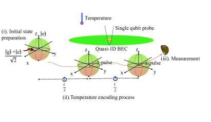
Figure 1: (color online) Schematic of the physical system under consideration: An atomic qubit is immersed in a thermally equilibrated quasi-1D BEC, which acts as a quantum sensor to estimate the temperature of the BEC. Our sensing protocol as following: (i) First we initialize the probe qubit in the superposition state $(|g\rangle+|e\rangle)/\sqrt{2}$, which is denoted by the Bloch sphere. (ii) Then the probe qubit undergoes a temperature encoding process via interacting with the BEC. (iii) Finally, choosing an optimal encoding time, we perform a measurement $\hat{\sigma}_{x}$ on the probe qubit, which can saturate the quantum Cramér-Rao bound.

As shown in Fig. 1, we consider a single impurity-atomic qubit immersed in a thermally equilibrated quasi-1D BEC at temperature $T$. The qubit is confined in a harmonic trap $V_{A}({\bf x})=m_{A}\omega_{A}^{2}{\bf x}^{2}/2$ that is independent of the internal states, where $m_{A}$ is the mass of the impurity and $\omega_{A}$ is the trap frequency. For $\hbar\omega_{A}\gg k_{B}T$, the spatial wave function of the qubit is the ground state of $V_{A}(\mathbf{x})$, i.e., $\varphi_{A}({\bf x})=\pi^{-3/4}\ell_{A}^{-3/2}\exp[-{\bf x}^{2}/(2\ell_{A}^{2})]$ with $\ell_{A}=\sqrt{\hbar/(m_{A}\omega_{A})}$. The Hamiltonian of the qubit is $\hat{H}_{A}=\Omega_{A}|e\rangle\langle e|$, where $\Omega_{A}$ is level splitting between the ground ($|g\rangle$) and excited ($|e\rangle$) states.

For the BEC, we assume that the gas is confined by a harmonic potential $V_{B}(\rho)=m_{B}\omega_{B}^{2}\rho^{2}/2$ in the x,y-directions($\rho^{2}=x^{2}+y^{2}$), where $\omega_{B}$ is the trap frequency. For sufficiently large $\omega_{B}$, the motion of the atoms along the $x$, $y$ axis is frozen to the ground state of $V_{B}(\rho)$, i.e., $\varphi_{B}(r)=\pi^{-1/2}\ell_{B}^{-1}\exp[-\rho^{2}/(2\ell_{B}^{2})]$ with $\ell_{B}=\sqrt{\hbar/(m_{B}\omega_{B})}$, which effectively reduces the BEC into a quasi-1D one. Finally, for small $T$, we may assume that most of the atoms are condensed to zero momentum state with a line density $n$. Then, following Bogoliubov’s method, the uncondensed atoms are described by the quasiparticle Hamiltonian

$$\hat{H}_{B}=\sum_{{\bf k}\neq 0}\epsilon_{\mathbf{k}}\hat{b}^{{\dagger}}_{{\bf k}}\hat{b}_{{\bf k}},$$ (1)

where $\hat{b}_{\mathbf{k}}$ is annihilation operator for the quasiparticle with the wave vector ${\mathbf{k}}$. Excitation energy $\epsilon_{\mathbf{k}}$ is

$$\epsilon_{\mathbf{k}}=\sqrt{E_{\mathbf{k}}^{2}+2ng_{B}E_{\mathbf{k}}}$$ (2)

where $E_{\mathbf{k}}=\hbar^{2}k^{2}/(2m_{B})$ is the kinetic energy and $g_{B}=2\hbar^{2}a_{B}/(m_{B}\ell_{B}^{2})$ is coupling constant with $a_{B}$ being the $s$-wave scattering length. In this work, we take the Bogoliubov Excitations in Eq. (1) as the reservoir of the qubit sensor.

For the sensor-reservoir coupling, the qubit probe undergoes spin-dependent $s$-wave collisions with the ultracold gas. We assume the qubit and the gas interact only when the qubit is in state $|e\rangle$ ,which can be achieved by tuning the scattering length for state $|g\rangle$ to zero via Feshbach resonance Chin2010 . Let $a_{AB}$ be the scattering length in state $|e\rangle$, the qubit-BEC interaction Hamiltonian is then

$$\hat{H}_{AB}=\delta_{e}|e\rangle\langle e|+|e\rangle\langle e|\sum_{\mathbf{k}\neq 0}g_{\mathbf{k}}\left(\hat{b}_{\mathbf{k}}+\hat{b}^{{\dagger}}_{\mathbf{k}}\right),$$ (3)

where $\delta_{e}=2\hbar^{2}na_{AB}/[m_{AB}(\ell^{2}_{A}+\ell^{2}_{B})]$ is the excited level shift due to the collision, $m_{AB}=m_{A}m_{B}/(m_{A}+m_{B})$ is the reduced mass, and the sensor-reservoir coupling parameter is

$$g_{\mathbf{k}}=\frac{\delta_{e}}{\sqrt{nL}}\sqrt{\frac{E_{\mathbf{k}}}{\epsilon_{\mathbf{k}}}}e^{-(\ell_{A}k)^{2}/4}$$ (4)

with $L$ being the size of the quasi-1D BEC .

Now the total Hamiltonian, $\hat{H}=\hat{H}_{A}+\hat{H}_{B}+\hat{H}_{AB}$, is

$$\hat{H}=(\Omega_{A}+\delta_{e})|e\rangle\langle e|+\sum_{{\mathbf{k}}\neq 0}\epsilon_{\mathbf{k}}\hat{b}^{{\dagger}}_{\mathbf{k}}\hat{b}_{\mathbf{k}}+|e\rangle\langle e|\sum_{\mathbf{k}\neq 0}g_{\mathbf{k}}\left(\hat{b}_{\mathbf{k}}+\hat{b}^{{\dagger}}_{\mathbf{k}}\right),$$ (5)

Since $\hat{H}_{A}$ commutes with $\hat{H}_{AB}$, the dynamics of the impurity qubit in reservoir is purely dephasing.

III Temperature sensing protocol by a dephasing qubit

As shown in Fig. 1, we consider the following temperature sensing protocol. (i) First we initialize the probe qubit in the superposition state $(|g\rangle+|e\rangle)/\sqrt{2}$, which is denoted by the Bloch sphere. (ii) Then the Probe qubit undergoes a temperature encoding process via interacting with the BEC. (iii) Finally, choosing an optimal encoding time, we perform a measurement $\hat{\sigma}_{x}$ on the probe qubit, which can saturate the quantum Cramér-Rao bound. Next we will specify the sensing protocol. The initial state of the total system is prepared as $(|g\rangle+|e\rangle)/\sqrt{2}\otimes\hat{\rho}_{B}(T)$, where $\hat{\rho}_{B}(T)=\prod_{\mathbf{k}}\left(1-e^{\beta\epsilon_{\mathbf{k}}}\right)e^{-\beta\epsilon_{\mathbf{k}}b_{{\mathbf{k}}}^{{\dagger}}b_{{\bf k}}}$ is a thermal state of the BEC, where $\beta=1/k_{B}T$ with $k_{B}$ and $T$ being the Boltzmann constant and temperature, respectively. Let the whole system evolve under the control of the Hamiltonian (5) for a certain time $t/2$, after which a $\pi$-pulse about $x$ is applied to the qubit. Then the system is allowed to evolve for the same time period $t/2$ and another $\pi$-pulse is applied. Through these processes, the quantum state of the qubit probe at time $t$ can be given as

$$\rho_{A}(t)=\frac{1}{2}\left(\begin{array}[]{cc}1&e^{-\Gamma(t,T)}\\ e^{-\Gamma(t,T)}&1\\ \end{array}\right),$$ (6)

where $\Gamma(t,T)$ is the dephasing factor with following expression

$$\Gamma(t,T)=\sum_{\mathbf{k}\neq 0}\frac{2g_{\mathbf{k}}^{2}}{\epsilon_{\mathbf{k}}^{2}}\sin\left(\frac{\epsilon_{\mathbf{k}}t}{2\hbar}\right)^{2}\coth\left(\frac{\epsilon_{\mathbf{k}}}{2k_{B}T}\right).$$ (7)

From above equation, one see the temperature information are encoded into the sensor’dephasing factor after encoding time $t$. Substituting $g_{\mathbf{k}}$ in Eq. (4) into above equation and using the continuum limit $\frac{1}{L}\sum_{\mathbf{k}}\rightarrow\frac{1}{\pi}\int^{\infty}_{0}dk$, we further obtain the dephasing factor as

$$\Gamma(t,T)=P\int^{\infty}_{0}dk\frac{e^{-(\ell_{A}k)^{2}/2}}{\epsilon_{\mathbf{k}}(E_{\mathbf{k}}+2ng_{B})}\sin\left(\frac{\epsilon_{\mathbf{k}}t}{2\hbar}\right)^{2}\coth\left(\frac{\epsilon_{\mathbf{k}}}{2k_{B}T}\right)$$ (8)

with the parameter $P=8n\hbar^{4}a_{AB}^{2}/[\pi m_{AB}^{2}\left(\ell^{2}_{A}+\ell^{2}_{B}\right)^{2}]$.

In the following, we introduce the quantum parameter estimate theory to quantify temperature sensing precision of the state in Eq. (6). As is well-known, the temperature sensing precision is restricted to the quantum Cramér-Rao bound

$$\delta T\geq\delta T_{QCR}\equiv\frac{1}{\sqrt{\nu\mathcal{F}^{Q}_{T}}}.$$ (9)

Here $\delta T$ is the mean square error, $\nu$ represents the number of repeated experiments and $\mathcal{F}^{Q}_{T}$ denotes quantum Fisher information (QFI) with respect to the temperature $T$. It is more convenient for a qubit to express QFI in Bloch representation. Any qubit state in the Bloch sphere representation can be written as $\hat{\rho}=1/2(\hat{I}+\mathbf{w}\cdot\mathbf{\hat{\sigma}})$, where $\hat{I}$ is $2$ identity matrix, $\mathbf{w}=(w_{x},w_{y},w_{z})^{T}$ is the real Bloch vector and $\mathbf{\hat{\sigma}}=(\hat{\sigma}_{x},\hat{\sigma}_{y},\hat{\sigma}_{z})$ represents the pauli matrices. The eigenvalues of the density operator $\rho$ can be given as $(1\pm w)/2$, where $w$ is the length of the Bloch vector. The length $w=1$ for pure state and $w<1$ for mixed state. In the Bloch sphere representation the QFI with respect to the estimated parameter $\lambda$ can be given as follows Wei2013 ; Jing2019

$$\mathcal{F}^{Q}_{\lambda}=\left\{\begin{array}[]{ll}\left|\partial_{\lambda}\mathbf{w}\right|^{2},&\hbox{$w=1;$}\\ \left|\partial_{\lambda}\mathbf{w}\right|^{2}+\frac{\left(\mathbf{w}\hskip 1.42271pt\cdot\hskip 1.42271pt\partial_{\lambda}\mathbf{w}\right)^{2}}{1-w^{2}},&\hbox{$w<1$.}\par\end{array}\right.,$$ (10)

where $\partial_{\lambda}$ denotes the derivative with respect to the estimated parameter $\lambda$. Therefore, to obtain the $\mathcal{F}^{Q}_{T}$ of the quantum state in Eq. (6) , we rewritten the quantum state as $\rho_{A}(t)=1/2(I+\mathbf{w}\cdot\mathbf{\sigma})$, where the Bloch vector $\mathbf{w}=(e^{-\Gamma},e^{-\Gamma},0)$. In the light of above equation, the concrete expression of the $\mathcal{F}^{Q}_{T}$ is obtained easily as follows

$$\mathcal{F}^{Q}_{T}=\frac{\left(\partial_{T}\Gamma\right)^{2}}{e^{2\Gamma}-1}.$$ (11)

The temperature sensing performance can be characterized by the QSNR

$$\mathcal{Q}_{T}=T^{2}\mathcal{F}^{Q}_{T}.$$ (12)

From the QCR bound in Eq. (9), the optimal relative error $(\delta T)_{min}/T$ and the QSNR $\mathcal{Q}_{T}$ has the following relation

$$\frac{(\delta T)_{min}}{T}=\frac{1}{\sqrt{\nu\mathcal{Q}_{T}}},$$ (13)

which means that the larger is the QSNR the better is the temperature sensing performance.

The last step of the temperature sensing protocol, we propose a measurement scheme at time $t$ which can saturate the quantum Cramér-Rao bound. For a two-level system, the Fisher information associated with the measurement can be presented as Mitchison2020

$$\mathcal{F}_{T}=\frac{1}{\langle\Delta\hat{X}^{2}\rangle}\left(\frac{\partial\langle\hat{X}\rangle}{\partial T}\right)^{2},$$ (14)

where $\langle\hat{X}\rangle$ and $\langle\Delta\hat{X}^{2}\rangle$ are mean and variance of the measured observable. The QFI is the upper bound of the Fisher information associated with the measurement $\hat{X}$, i.e., $\mathcal{F}^{Q}_{T}=\max_{\hat{X}}\mathcal{F}_{T}(\hat{X})=\mathcal{F}_{T}(\hat{\Lambda})$. It is very important to find an optimal measurement $\hat{\Lambda}$ for experimental implementation. In this work we choose $\langle\hat{\sigma}_{x}\rangle$ as the measurement signal, which can be observed using Ramsey interferometry Adam2022- ; Scelle2013 ; Cetina2016 .

Based on the quantum state of the single-atom temperature sensor given by Eq. (6), it is straightforward to obtain

$$\langle\hat{\sigma}_{x}\rangle=e^{-\Gamma},\hskip 5.69046pt\langle\Delta\hat{\sigma}_{x}^{2}\rangle=1-e^{-2\Gamma}.$$ (15)

The Fisher information associated with the measurement $\hat{\sigma}_{x}$ is obtained by substituting above equation into Eq. (14)

$$\mathcal{F}_{T}(\sigma_{x})=\frac{\left(\partial_{T}\Gamma\right)^{2}}{e^{2\Gamma}-1},$$ (16)

which is exactly eqaul to the quantum Fisher information given by Eq. (11). Therefore, we can conclude that the sensitivity of the temperature sensor in present scheme can saturate the quantum Cramér-Rao bound through performing the measurement $\hat{\sigma}_{x}$ on the probe qubit

IV Numerical results of the temperature sensing performance

In this section we investigate numerically the temperature sensing performance via studying the dynamics of QSNR. For facilitating the procedure of numerical calculation, we transfer the parameters in the dephasing factor in Eq. (8) into dimensionless form as

$$\Gamma(\tilde{t},\tilde{T})=\tilde{P}\int^{\infty}_{0}d\tilde{k}\frac{e^{\frac{-(\sigma\tilde{k})^{2}}{2}}}{\tilde{\epsilon}_{\mathbf{k}}(\tilde{k}^{2}+2\alpha)}\sin\left(\frac{\tilde{\epsilon}_{\mathbf{k}}\tilde{t}}{2\tilde{T}}\right)^{2}\coth\left(\frac{\tilde{\epsilon}_{\mathbf{k}}}{2\tilde{T}}\right),$$ (17)

where the dimensionless parameter $\tilde{P}=32na_{AB}^{2}(m_{A}+m_{B})^{2}/\left[\pi\ell_{B}m_{A}^{2}(1+\sigma^{2})^{2}\right]$ with $\sigma=\ell_{A}/\ell_{B}$, the dimensionless wave vector $\tilde{k}=\ell_{B}k$, excitation energy $\tilde{\epsilon}_{\mathbf{k}}=\sqrt{\tilde{k}^{4}+2\alpha\tilde{k}^{2}}$ with $\alpha=4na_{B}$ ,time $\tilde{t}=\omega_{T}t$ with $\omega_{T}=k_{B}T/\hbar$ and temperature $\tilde{T}=2k_{B}T/(\hbar\omega_{B})$. To present our results, we consider a single ²³Na atom with the mass $m_{A}\approx 3.82\times 10^{-26}$kg immersed in a ⁸⁷Rb BEC with the atomic mass $m_{B}\approx 14.45\times 10^{-26}$kg. We assume a typical trap frequency $\omega_{B}=2\pi\times 10^{3}\,{\rm Hz}$, the corresponding harmonic oscillator width is $\ell_{B}\simeq 3.4\times 10^{-5}\,{\rm cm}$. Next, we consider a typical condensate peak density of $10^{14}\,{\rm cm}^{-3}$, the line density is then $n=3.6\times 10^{5}\,{\rm cm}^{-1}$. In this work, the scattering length of the BEC takes its nature value of $a_{B}=a_{Rb}\approx 5.3$nm and the dimensionless parameter $\sigma$ is given by $\sigma=0.5$. When it is not a variable, we take the scattering length $a_{AB}=55a_{0}\approx 2.9$nm with $a_{0}$ being the Bohr radiusHaikka2011 . Consequently, we have $\tilde{P}\approx 0.13$ and $\alpha\approx 0.77$.

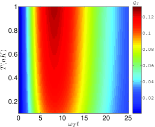
Figure 2: (color online) The QSNR as a function of dimensionless time $\omega_{T}t$ and temperature $T$.The values of relevant parameters are shown in the first paragraph of section IV.

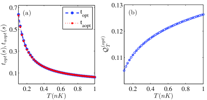
Figure 3: (Color online) (a) Comparision of the numerical optimal encoding time $t_{opt}$ and the approximate optimal encoding time $t_{aopt}=8.2/\omega_{T}$. (b) The optimal QSNR $\mathcal{Q}^{(opt)}_{T}$ as a function of the temperature $T$.

Figure 2 plots the dynamical behaviors of the QSNR in the sub-nK range from $0.1$ nK to $1$ nK. It is shown the QSNR increases firstly and then decreases with time for full temperature range. This means that for a given temperature there is an optimal encoding time $t_{opt}$ that the QSNR reaches its maximum, which is called optimal QSNR $\mathcal{Q}^{(opt)}_{T}$. Moreover, figure 2 reveals that the optimal encoding time $t_{opt}$ may satisfy the following relation

$$\omega_{T}t_{opt}=R,$$ (18)

where $R$ is a temperature-independent parameter. It follows that the optimal encoding time is inversely proportional to the temperature. To confirm this, Figure 3(a) compares the numerical optimal encoding time $t_{opt}$ and the approximate optimal encoding time $t_{aopt}=8.2/\omega_{T}$. As can be seen, the agreement is remarkable. Figure 3(b) corresponds to the maximal QSNR $\mathcal{Q}^{(opt)}_{T}$ as a function of the temperature $T$. It is a natural result that the optimal QSNR increases with temperature.

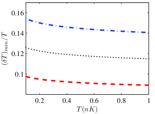
Figure 4: (Color online) The optimal relative error $(\delta T)_{min}/T$ as a function of temperature $T$ after 400 (blue, dash-dotted), 600(black, dotted) and 1000(red, dashed) measurements.

Figure 4 plots the optimal relative error $(\delta T)_{min}/T$ as a function of temperature $T$ after 400 (blue, dash-dotted), 600(black, dotted) and 1000(red, dashed) measurements. We can see in the sub-nk regime the optimal relative error is insensitive to temperature changes, which is different from the sensing schemes of the sub-nK temperature being encoded into the qubit’s relative phase White2014 or the harmonic oscillator’s position quadrature Mehboudi2019 ; Khan2022- . In these schemes, as temperature decreases from $0.3$ nK, the upward tendency of the optimal relative error will become apparent. This implies our scheme may be more suitable for designing sub-nK-lower quantum sensor. From Fig. (4), one can see with only 400 measurements, the optimal relative error can be kept below $16\%$ for full temperatures( see blue dash-dotted line ). As the number of the measurements increases to $1000$ , the optimal relative error will drop below $10\%$ (see red dashed line). For the temperature sensing performance, the qubit sensor is comparable to the harmonic oscillator sensor in the sub-nk regime Mehboudi2019 ; Khan2022- .

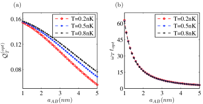
Figure 5: (Color online) (a) The optimal QSNR $\mathcal{Q}^{(opt)}_{T}$ as a function of the scattering length $a_{{}_{AB}}$ for $0.2nK$, $0.5nK$ and $0.8nK$. (b) The dimensionless optimal encoding time $\omega_{T}t_{opt}$ as a function of the scattering length $a_{{}_{AB}}$ for $0.2nK$, $0.5nK$ and $0.8nK$. Other related parameters are the same as in Fig. 2.

In the following, we study the effects of the coupling strength between the sensor and the BEC on the optimal QSNR and the optimal encoding time. From Eq. (4), we see the coupling strength can be well controlled by adjusting the scattering length $a_{{}_{AB}}$ via Feshbach resonance Chin2010 . Therefore, figure 5(a) plots the optimal QSNR $\mathcal{Q}^{(opt)}_{T}$ as a function of the scattering length $a_{{}_{AB}}$ for $0.2nK$, $0.5nK$ and $0.8nK$. It is shown the optimal QSNR $\mathcal{Q}^{(opt)}_{T}$ decreases as increases the scattering length $a_{{}_{AB}}$ for all temperatures. It is demonstrated that weaker coupling can enhance temperature sensing precision, which also holds in the temperature sensing process of a dephasing qubit immersed in a cold Fermi gas Mitchison2020 , but is contrary for a harmonic oscillator probe, where strong coupling is considered as a resource to enhance the temperature sensing precision Correa2017 . More interestingly, as the scattering length $a_{{}_{AB}}$ decreases to $1$nm, all optimal QSNRs increase to the same value. This implies there may be a temperature-independent upper limit value of the QSNR when the scattering length $a_{{}_{AB}}$ is small enough. Corresponding, the optimal encoding time $\omega_{T}t_{opt}$ is shown in Fig. 5(b). As can be seen, the optimal time $\omega_{T}t_{opt}$ increases with decreaseing the scattering length $a_{{}_{AB}}$. Moreover, the three curves for $0.2nK$, $0.5nK$ and $0.8nK$ overlap very well, which indicates the equation (18) still holds for different coupling strengths and only the temperature-independent parameter $R$ increases with decreasing the scattering length $a_{{}_{AB}}$. Combining Fig. 5(a) and Fig.  5(b), we see there is a trade-off between optimal QSNR and optimal encoding time, which is controlled by the scattering length $a_{{}_{AB}}$. The price of obtaining larger optimal QSNR has to pay longer optimal encoding time.

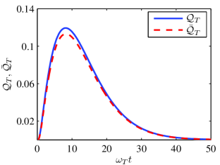
Figure 6: (Color online) Comparison the time evolution of the numerical QSNR $\mathcal{Q}_{T}$ and the analytical QSNR $\bar{\mathcal{Q}}_{T}$ in Eq.(22). The temperature $T=0.5nK$, other related parameters are the same as in Fig. 2.

V Analytical results of the temperature sensing performance

In this section, we study analytically the temperature sensing performance of the dephasing qubit and try to give an analysis of above numerical results under some approximations. For the wave vector $k\ll\xi^{-1}=\sqrt{m_{B}ng_{B}}/\hbar$ with $\xi$ being the healing length, the excitations of the BEC are phonons with the dispersion relation $\epsilon_{\mathbf{k}}=\hbar c_{s}k$, where $c_{s}=\sqrt{ng_{B}/m_{B}}$ is the velocity of sound. We notice the phonon excitations make the major contributions for the time evolution of the QSNR. Therefore, as an approximation, in the full wave vector region, we substitute the phonon dispersion relation $\epsilon_{\mathbf{k}}=\hbar c_{s}k$ into the sensor-reservoir coupling parameter $g_{\mathbf{k}}$ in Eq. (4) and obtain an analytical expression of reservoir spectrum density function $J(\omega)\equiv\sum_{\mathbf{k}}|g_{\mathbf{k}}|^{2}\delta(\omega-\omega_{\mathbf{k}})$ as

$$J(\omega)=\eta\omega e^{-\frac{\omega^{2}}{\omega_{c}^{2}}},$$ (19)

where the dimensionless reservoir coupling parameter

$$\eta=\frac{na_{AB}^{2}\ell_{B}^{3}(m_{A}+m_{B})^{2}}{\sqrt{2}\pi(\ell_{A}^{2}+\ell_{B}^{2})^{2}m_{A}^{2}}\left(\frac{1}{na_{B}}\right)^{\frac{3}{2}}$$ (20)

and the cutoff frequency $\omega_{c}=\sqrt{2}c_{s}/\ell_{A}$. From Eq. (20), we see the reservoir coupling parameter $\eta$ is proportional to the square of the scattering length $a_{AB}$ . It is worth noting that the scattering length $a_{AB}$ only appears in the dimensionless reservoir coupling parameter $\eta$ in our model. So adjusting the scattering length $a_{AB}$ is equivalent to controlling the reservoir coupling parameter $\eta$. For $1$ nm $\leq a_{AB}\leq 5$nm, the reservoir coupling parameter $\eta$ is in the range of $0.004\leq\eta\leq 0.1$ with related parameters being the same as in Fig. 2. For getting a concrete analytical expression of the QSNR, we further approximate the spectrum density function as the standard Ohmic spectrum density $J(\omega)=\eta\omega e^{-\frac{\omega}{\omega_{c}}}$ Benedetti2018 ; Sehdaran2019 ; Tan2022 . Then under condition $\omega_{c}/\omega_{T}>>1$ (in our model, $\omega_{c}/\omega_{T}=84$ for $T=1nK$ ), the dephasing factor is given as

$$\bar{\Gamma}=\frac{\eta}{2}\ln(1+\omega_{c}^{2}t^{2})+\eta\ln\left[\frac{1}{\pi\omega_{T}t}\sinh(\pi\omega_{T}t)\right].$$ (21)

Substituting above equation into Eqs. (11) and (12), we find QSNR analytically that

$$\bar{\mathcal{Q}}_{T}=\frac{\eta^{2}\left[\pi\omega_{T}t\coth(\pi\omega_{T}t)-1\right]^{2}}{(1+\omega_{c}^{2}t^{2})^{\eta}\left[\frac{1}{\pi\omega_{T}t}\sinh(\pi\omega_{T}t)\right]^{2\eta}-1}.$$ (22)

In Fig. (6), we compare the time evolution of the numerical QSNR $\mathcal{Q}_{T}$ and the analytical QSNR $\bar{\mathcal{Q}}_{T}$ in Eq. (22) with $T=0.5$ nK. As can be seen, except for the slight difference at maximum point, the agreement is remarkable. In fact, such agreement still holds for other temperatures.

Now according to the analytical expression of QSNR $\bar{\mathcal{Q}}_{T}$, we would like to provide an analytical description of the numerical results obtained. We firstly analyze the QSNR varying with time. In order to find the extreme-value point $\bar{t}_{opt}$, we take the derivative of QSNR $\bar{\mathcal{Q}}_{T}$ with respect time $t$. We shall analytically indicate that there exists an optimal encoding time $\bar{t}_{opt}$. When $t<\bar{t}_{opt}$, the derivative $\partial\bar{\mathcal{Q}}_{T}/\partial t>0$, otherwise, $\partial\bar{\mathcal{Q}}_{T}/\partial t<0$. Therefore, as shown in Fig. 2, the QSNR increases firstly then decreases with time. We further find, under the conditions of $\omega_{c}\bar{t}_{opt}>>1$ and $\pi\omega_{T}\bar{t}_{opt}>>1$ ( the conditions are well satisfied, see the numerical results in Fig. 5 (b)), the optimal encoding time satisfies the following equation

$$\omega_{T}\bar{t}_{opt}=\frac{1}{\pi\eta}\left(1-\frac{1}{\zeta_{T}^{2\eta}e^{2\pi\eta\omega_{T}\bar{t}_{opt}}}\right),$$ (23)

where $\zeta_{T}=\omega_{c}/(2\pi\omega_{T})$.

In the following, we shall analyze the optimal encoding time $\bar{t}_{opt}$ as the function of the temperature and the scattering length $a_{AB}$. We will analytically indicate why $\omega_{T}t_{opt}$ can be approximated as a temperature-independent parameter $R$ in Eq. (18) and whether there is a concrete expression of $R$, which matches the behavior in Fig. 5 (b). We rewrite Eq. (23) as the following form

$$\omega_{T}\bar{t}_{opt}=\frac{1}{\pi\eta}\left(1-z-2z^{2}+o(z^{3})\right),$$ (24)

where $z$ is a temperature-dependent parameter with following form

$$z(T)=\frac{1}{e^{2}}\left(\frac{2\pi k_{B}T}{\hbar\omega_{c}}\right)^{2\eta}.$$ (25)

Above equation shows the parameter $z$ is an increasing function of temperature $T$ and decreasing function of reservoir coupling parameter $\eta$ due to $2\pi k_{B}T/\hbar\omega_{c}<1$. Substituting the values of related parameters in the first paragraph of section IV into Eq. ( 25), we obtain $0.05\leq z\leq 0.13$ in the temperature range of $0.1nK\leq T\leq 1nK$ and $1nm\leq a_{AB}\leq 5nm$. The temperature-dependent parameter $z$ can be further made Taylor series expansion of temperature at temperature $T_{0}$ as $z=z(T_{0})+2\eta(T-T_{0})/T_{0}+o(\eta^{2})$. In the sub-nK regime, we take $T_{0}=0.5nK$, then obtain $|(T-T_{0})/T_{0}|\leq 1$ and $z(T_{0})=1/(e^{2}27^{2\eta})$. Due to $\eta$ being a small quantity and $z$ itself also a small quantity in Eq. (24), it is reasonable to substitute $z\approx z(T_{0})=1/(e^{2}27^{2\eta})$ into Eq. (24) and obtain

$$\omega_{T}\bar{t}_{opt}=\bar{R}=\frac{1}{\pi\eta}\left[1-z(T_{0})-2z^{2}(T_{0})+o\left(z^{3}(T_{0})\right)\right].$$ (26)

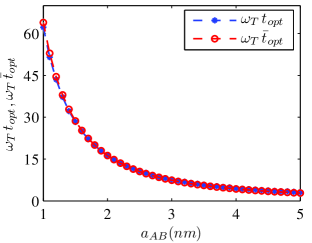
Figure 7: (Color online) Comparison the numerical optimal encoding time $\omega_{T}t_{opt}$ and the analytical optimal encoding time $\omega_{T}\bar{t}_{opt}$ in Eq. (26) as a function of the scattering length $a_{{}_{AB}}$.

In Fig. 7 we make a comparison between the numerical optimal encoding time $\omega_{T}t_{opt}$ and the analytical optimal encoding time $\omega_{T}\bar{t}_{opt}$ in Eq. (26) as a function of the scattering length $a_{{}_{AB}}$. Figure. 7 indicates the good agreement between the numerical and analytical optimal encoding time and $R=\bar{R}$.

We now analytically investigate the influence of the temperature and the scattering length $a_{AB}$ on the optimal QSNR. Substituting the analytically optimal encoding time given by Eq. (24) into Eq. (22), we can obtain the analytically optimal QSNR $\bar{\mathcal{Q}}^{(opt)}_{T}$ with the following expression

$$\bar{\mathcal{Q}}^{(opt)}_{T}=(1-2\eta)z+(1-4\eta)z^{2}+2(1-6\eta)z^{3}+o(z^{4}).$$ (27)

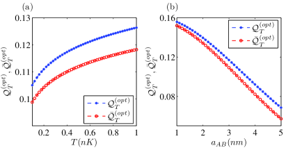
Figure 8: (Color online) (a) Comparison the numerical optimal QSNR $\mathcal{Q}^{(opt)}_{T}$ and the analytical optimal QSNR $\bar{\mathcal{Q}}^{(opt)}_{T}$ in Eq. (27) as a function of temperature. the scattering length $a_{AB}$ is taken as $2.9nm$. (b) Comparison the numerical optimal QSNR $\mathcal{Q}^{(opt)}_{T}$ and the analytical optimal QSNR $\bar{\mathcal{Q}}^{(opt)}_{T}$ in Eq. (27) as a function of scattering length $a_{AB}$. the temperature is taken as $T=0.5nK$.

In order to compare the analytical and numerical results of the optimal QSNR, we have plotted the analytically and numerically optimal QSNR as a function of temperature and the scattering length in Fig. 8(a) and Fig. 8(b), respectively. From Fig. 8(a) and Fig. 8(b), we can see that the analytical optimal QSNR is highly consistent with the numerical optimal QSNR. In particular, the lower the temperature is or the smaller the scattering length is, the better the consistency between the analytical and numerical results is.

We now analytically study the optimal QSNR in the weak coupling limit and show that the optimal QSNR can tend to the same value which is independent of temperature when the scattering length decreases to the $1nm$ scale. Specifically, the reservoir coupling parameter $\eta$ becomes very small, $\eta\approx 0.004$, as the scattering length $a_{AB}=1nm$. In this case, the temperature-dependent parameter $z$ in Eq. (25) becomes very insensitive to temperature. In fact, when $\eta=0.004$, it is calculated as $z(T=1nK)=0.132$ and $z(T=0.1nK)=0.130$, which shows the temperature effects on the optimal QSNR in Eq. (27) becomes negligible. Thanks to the parameter $z$ being a decreasing function of reservoir coupling parameter $\eta$, one can conclude from Eq. (27) that the optimal QSNR is a decreasing function of reservoir coupling parameter $\eta$. This means weaker coupling can enhance the temperature sensing precision as shown in Fig. 5(a). Inspiring by these analyses, based on Eq. (27), we can get an upper bound of the QSNR as

$$\mathcal{Q}_{T}^{up}=\lim_{\eta\rightarrow 0}\bar{\mathcal{Q}}_{T}^{(opt)}=\frac{1}{e^{2}}+\frac{1}{e^{4}}+\frac{2}{e^{6}}+o\left(\frac{1}{e^{8}}\right)\approx 0.16,$$ (28)

which is applicable in the range of $T<<\hbar\omega_{c}/k_{B}$ and $\eta<<1$ for an Ohmic reservoir. It is worth noting for arbitrarily low temperature, as long as the $\eta$ is small enough, the QSNR also can close to the upper bound $\mathcal{Q}_{T}^{up}$. This can be understood from the dynamics of quantum coherence of the temperature sensor. Figure 9 plots the dynamics of quantum coherence $|\rho^{(A)}_{eg}|$ for $0.01nK$, $0.03nK$ and $0.05nK$. It is demonstrated that the dynamics is still sensitive with sub-nK-lower temperature change, although the sensitivity takes longer to be prominent.

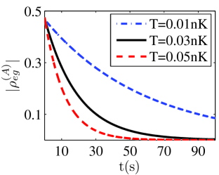
Figure 9: (Color online) The dynamics of quantum coherence $|\rho^{(A)}_{eg}|$ of the sensor for $0.01nK$, $0.03nK$ and $0.05nK$. The dimensionless reservoir coupling parameter $\eta=0.004$.

Finally, we analytically discuss the behaviors of optimal QSNR when temperature is close to absolute zero. It is well known that for the thermal equilibrium probes, the QSNR satisfies $\mathcal{Q}_{T}\sim e^{-\Delta/(k_{B}T)}$ with $\Delta$ being energy gap, which indicates the QSNR will decay exponentially fast to zero in the limit $T\rightarrow 0$, and for a non-thermal equilibrium harmonic oscillator probe, a quartic scaling law $\mathcal{Q}_{T}\sim T^{4}$ can be achieved, which demonstrates QSNR still decays to zero in the limit $T\rightarrow 0$  Hovhannisyan2018 ; Potts2019 ; Potts2020 . In our model, according to Eqs. (25) and (27), we can obtain the scaling law $\bar{\mathcal{Q}}_{T}^{(opt)}\sim T^{2\eta}$ in the limit $T\rightarrow 0$. This implies that when the parameter $\eta$ approaches to zero, one can prevent the optimal QSNR from decaying to zero as the temperature is close to absolute zero. As a matter of fact, in the weak coupling limit, using the limit relation $\lim_{x,y\rightarrow 0}x^{y}=1$, we can obtain

$$\lim_{\eta,T\rightarrow 0}\bar{\mathcal{Q}}_{T}^{(opt)}=\mathcal{Q}_{T}^{up},$$ (29)

where the upper bound of the QSNR $\mathcal{Q}_{T}^{up}$ is given by Eq. (28). Therefore, we can conclude that the temperature sensing error in our model does not diverge as temperature is close to absolute zero in the weak coupling limit. We should point out the weak coupling, selecting optimal encoding time to achieve the optimal QSNR, and sensitivity of dephasing dynamics on the ultra-low temperature change are responsible for avoiding the error-divergence in our model.

VI Conclusions

In conclusion, we have studied the quantum sensing scheme of temperature close to absolute zero in a quasi-one-dimensional BEC. We have demonstrated that the sensitivity of the temperature sensor can saturate the quantum Cramér-Rao bound by means of measuring quantum coherence of the probe qubit, and weaker coupling between the probe qubit and the BEC can enhance the temperature sensing precision. We have investigated numerically and analytically the temperature sensing performance. It has been indicated that there is an optimal encoding time in which the QSNR can reach its maximum in the full-temperature regime. In particular, it has been found that the QSNR can reach a finite temperature-independent upper bound under the weak coupling condition even when the temperature is close to absolute zero. This implies that the sensing-error-divergence problem is avoided in our scheme. It has been shown that weak coupling, selecting optimal encoding time and sensitive dephasing dynamics on the ultra-low temperature change are responsible for avoiding the error-divergence. Our work opens a way for quantum sensing of temperature close to absolute zero in the BEC.

- (1) F. Giazotto, T. T. Heikkilä, A. Luukanen, A. M. Savin, and J. P. Pekola, Opportunities for mesoscopics in thermometry and refrigeration: Physics and applications, Rev. Mod. Phys. 78, 217 (2006).
- (2) M. Mehboudi, A. Sanpera, and L. A. Correa, Thermometry in the quantum regime: recent theoretical progress, J. Phys. A: Math. Theor. 52, 303001 (2019).
- (3) A. Leanhardt, T. Pasquini, M. Saba, A. Schirotzek, Y. Shin, D. Kielpinski, D. Pritchard, and W. Ketterle, Cooling Bose-Einstein condensates below 500 picokelvin, Science 301, 1513 (2003).
- (4) R. Gati, B. Hemmerling, J. Fölling, M. Albiez, and M. K. Oberthaler, Noise Thermometry with Two Weakly Coupled Bose-Einstein Condensates, Phys. Rev. Lett. 96, 130404 (2006).
- (5) R. Gati, J. Esteve, B. Hemmerling, T. Ottenstein, J. Appmeier, A. Weller, and M. Oberthaler, A primary noise thermometer for ultracold Bose gases, New J. Phys. 8, 189 (2006).
- (6) R. Olf, F. Fang, G. E. Marti, A. MacRae, and D.M. Stamper-Kurn, Thermometry and cooling of a Bose-Einstein condensate to 0.02 times the critical temperature, Nat. Phys. 11, 720 (2015).
- (7) M. Brunelli, S. Olivares, and M. G. A. Paris, Qubit thermometry for micromechanical resonators, Phys. Rev. A 84, 032105 (2011).
- (8) M. Brunelli, S. Olivares, M. Paternostro, and M. G. A. Paris, Qubit-assisted thermometry of a quantum harmonic oscillator, Phys. Rev. A 86, 012125 (2012).
- (9) C. Sabín, A. White, L. Hackermuller, and I. Fuentes, Impurities as a quantum thermometer for a Bose-Einstein condensate, Sci. Rep. 4, 6436 (2014).
- (10) S. Jevtic, D. Newman, T. Rudolph, and T. M. Stace, Single-qubit thermometry, Phys. Rev. A 91, 012331 (2015).
- (11) L. Seveso and M. G. A. Paris, Trade-off between information and disturbance in qubit thermometry, Phys. Rev. A 97, 032129 (2018).
- (12) S. Razavian, C. Benedetti, M. Bina, Y. Akbari-Kourbolagh, and M. G. A. Paris, Quantum thermometry by single-qubit dephas- ing, Eur. Phys. J. Plus 134, 284 (2019).
- (13) M. T. Mitchison, T. Fogarty, G. Guarnieri, S. Campbell, T. Busch, and J. Goold, In situ thermometry of a cold fermi gas via dephasing impurities, Phys. Rev. Lett. 125, 080402 (2020).
- (14) M. Mehboudi, A. Lampo, C. Charalambous, L. A. Correa, M. Á. García-March, and M. Lewenstein, Using Polarons for sub-nK Quantum Nondemolition Thermometry in a Bose-Einstein Condensate, Phys. Rev. Lett. 122, 030403 (2019).
- (15) M. M. Khan, M. Mehboudi, H. Terças, M. Lewenstein, and M. A. Garcia-March, Subnanokelvin thermometry of an interacting -dimensional homogeneous Bose gas, Phys. Rev. Research 4, 023191 (2022).
- (16) M. Miskeen Khan, H. Terccas, J. T. Mendonca, J. Wehr, C. Charalambous, M. Lewenstein, and M. A. Garcia- March, Quantum dynamics of a bose polaron in a d-dimensional bose-einstein condensate, Phys. Rev. A 103, 023303 (2021).
- (17) U. Marzolino and D. Braun, Precision measurements of temperature and chemical potential of quantum gases,Phys. Rev. A 88, 063609 (2013)
- (18) E. Martín-Martínez, A. Dragan, R. B. Mann, and I. Fuentes, Berry phase quantum thermometer, New J. Phys. 15, 053036 (2013).
- (19) M. Mehboudi, M. Moreno-Cardoner, G. De Chiara, and A. Sanpera, Thermometry precision in strongly correlated ultracold lattice gases, New Journal of Physics 17, 055020 (2015).
- (20) M. Hohmann, F. Kindermann, T. Lausch, D. Mayer, F. Schmidt, and A. Widera, Single-atom thermometer for ultracold gases, Phys. Rev. A 93, 043607 (2016).
- (21) T. H. Johnson, F. Cosco, M. T. Mitchison, D. Jaksch, and S. R. Clark, Thermometry of ultracold atoms via nonequilibrium work distributions, Phys. Rev. A 93, 053619 (2016).
- (22) S. Seah, S. Nimmrichter, D. Grimmer, J. P. Santos, V. Scarani, and G. T. Landi, Collisional Quantum Thermometry, Phys. Rev. Lett. 123, 180602 (2019).
- (23) D. Tamascelli, C. Benedetti, H. P. Breuer, and M. G. A. Paris, Quantum probing beyond pure dephasing, New Journal of Physics 22, 083027 (2020).
- (24) L. Mancino, M. G. Genoni, M. Barbieri, and M. Paternostro, Nonequilibrium readiness and precision of Gaussian quantum thermometers, Phys. Rev. Research 2, 033498 (2020).
- (25) A. V. Kirkova, W. Li, and P. A. Ivanov, Adiabatic sensing technique for optimal temperature estimation using trapped ions, Phys. Rev. Research 3, 013244 (2021).
- (26) J. Rubio, J. Anders, and L. A. Correa, Global Quantum Thermometry, Phys. Rev. Lett. 127, 190402 (2021).
- (27) L. Oghittu and A. Negretti,Quantum-limited thermometry of a Fermi gas with a charged spin particle, Phys. Rev. Research 4, 023069 (2022).
- (28) D. Adam, Q. Bouton, J. Nettersheim, S. Burgardt, and A. Widera, Coherent and Dephasing Spectroscopy for Single-Impurity Probing of an Ultracold Bath,Phys. Rev. Lett. 129, 120404 (2022).
- (29) T.M. Stace, Quantum limits of thermometry, Phys. Rev. A 82, 011611 (2010).
- (30) A. Candeloro and M. G. A. Paris, Discrimination of ohmic thermal baths by quantum dephasing probes, Phys. Rev. A 103, 012217 (2021).
- (31) F. Gebbia, C. Benedetti, F. Benatti, R. Floreanini, M. Bina, and M. G. A. Paris, Two-qubit quantum probes for the temperature of an ohmic environment, Phys. Rev. A 101, 032112(2020).
- (32) H. Ather and A. Z. Chaudhry, Improving the estimation of environment parameters via initial probe-environment correlations, Phys. Rev. A 104, 012211 (2021).
- (33) L. T. Kenfack, W. D. W. Gueagni, M. Tchoffo, and L. CorneliusFai, Temperature estimation in a quantum spin bath through entangled and separable two-qubit probes, The European Physical Journal Plus 136, 220 (2021).
- (34) G. Planella, M. F. B. Cenni, A. Acin, and M. Mehboudi, Bath-Induced Correlations Enhance Thermometry Precision at Low Temperatures, Phys. Rev. Lett. 128, 040502 (2022).
- (35) Z. Z. Zhang and W. Wu, Non-Markovian temperature sensing, Phys. Rev. Research 3, 043039 (2021).
- (36) W. Wu, S. Y. Bai, and J. H. An, Non-Markovian Sensing of a Quantum Reservoir, Phys. Rev. A 103, 010601 (2021).
- (37) N. Zhang, C. Chen, S. Y. Bai, W. Wu, and J. H. An, Non-Markovian quantum thermometry, Phys. Rev. Applied 17, 034073 (2022).
- (38) L. A. Correa, M. Perarnau-Llobet, K. V.Hovhannisyan, S. Hernández-Santana, M. Mehboudi, and A. Sanpera, Enhancement of low-temperature thermometry by strong coupling, Phys.Rev. A 96, 062103 (2017).
- (39) J. Glatthard and L. A. Correa, Bending the rules of low-temperature thermometry with periodic driving, arXiv:2203.02436v3(2022).
- (40) A. H. Kiilerich, A. De Pasquale, and V. Giovannetti, Dynamical approach to ancilla-assisted quantum thermometry, Phys. Rev. A 98, 042124 (2018).
- (41) M. M. Feyles, L. Mancino, M. Sbroscia, I. Gianani, and M. Barbieri, Dynamical role of quantum signatures in quantum thermometry, Phys. Rev. A 99, 062114 (2019).
- (42) V. Mukherjee, A. Zwick, A. Ghosh, X. Chen, and G. Kur-izki, Enhanced precision bound of low-temperature quan- tum thermometry via dynamical control, Commun. Phys. 2, 162 (2019).
- (43) I. Bloch, J. Dalibard, and W. Zwerger,Many-body physics with ultracold gases, Rev. Mod. Phys. 80, 885 (2008).
- (44) I. Bloch, J. Dalibard, and S. Nascimbene, Quantum simulations with ultracold quantum gases, Nat. Phys. 8, 267 (2012).
- (45) D. Reeb and M. M. Wolf, Tight bound on relative entropy by entropy difference, IEEE Trans. Inf. Theory 61, 1458 (2015).
- (46) L. A. Correa, M. Mehboudi, G. Adesso,and A. Sanpera, Individual quantum probes for optimal thermometry, Phys. Rev. Lett. 114, 220405 (2015).
- (47) Matteo G A Paris, Achieving the landau bound to precision of quantum thermometry in systems with vanishing gap, Journal of Physics A: Mathematical and Theoretical 49, 03LT02 (2015).
- (48) K. V. Hovhannisyan and L. A. Correa, Measuring the temperature of cold many-body quantum systems, Phys. Rev. B 98, 045101 (2018).
- (49) P. P. Potts, J. B. Brask, and N. Brunner, Fundamental limits on low-temperature quantum thermometry with finite resolution, Quantum 3, 161 (2019).
- (50) M. R. Jørgensen , P. P. Potts , M. G. A. Paris , and J. B. Brask, Tight bound on finite-resolution quantum thermometry at low temperatures, Phys. Rev. Research 3, 033394 (2020).
- (51) A. Recati, P.O. Fedichev, W. Zwerger, J. von Delft, and P. Zoller, Atomic Quantum Dots Coupled to a Reservoir of a Superfluid Bose-Einstein Condensate, Phys. Rev. Lett. 94, 040404 (2005).
- (52) M. A. Cirone, G. De Chiara, G. M. Palma, and A. Recati, Collective decoherence of cold atoms coupled to a Bose-Einstein condensate, New J. Phys. 11, 103055 (2009).
- (53) Y. J. Song and L. M. Kuang, Controlling Decoherence Speed Limit of a Single Impurity Atom in a Bose-Einstein-Condensate Reservoir, Ann. Phys. 531, 1800423 (2019).
- (54) H. P. Breuer and F. Petruccione, The Theory of Open Quantum Systems (Oxford University Press, Oxford, 2007).
- (55) L. M. Kuang, H. S. Zeng, and Z. Y. Tong, Nonlinear decoherence in quantum state preparation of a trapped ion, Phys. Rev. A 60, 3815 (1999).
- (56) L. M. Kuang, Z. Y. Tong, Z. W Ouyang, and H. S. Zeng, Decoherence in two Bose-Einstein condensates, Phys. Rev. A 61, 013608 (1999).
- (57) P. Haikka, S. McEndoo, G. De Chiara, G. M. Palma, and S. Maniscalco, Quantifying, characterizing, and controlling information flow in ultracold atomic gases, Phys. Rev. A 84, 031602(R) (2011).
- (58) P. Haikka, S. McEndoo, and S. Maniscalco, Non-Markovian probes in ultracold gases, Phys. Rev. A 87, 012127 (2013).
- (59) J. B. Yuan, H. J. Xing, L. M. Kuang, and S. Yi, Quantum non-Markovian reservoirs of atomic condensates engineered via dipolar interactions, Phys. Rev. A 95, 033610 (2017).
- (60) D. Hangleiter, M. T. Mitchison, T. H. Johnson, M. Bruderer, M. B. Plenio, and D. Jaksch, Nondestructive selective probing of phononic excitations in a cold Bose gas using impurities, Phys. Rev. A 91, 013611 (2015).
- (61) L. Mancino, M. Sbroscia, I. Gianani, E. Roccia, and M. Barbieri, Quantum Simulation of Single-Qubit Thermometry Using Linear Optics, Phys. Rev. Lett. 118, 130502 (2017).
- (62) P.P. Hofer, J. B. Brask, M. Perarnau-Llobet, and N. Brunner, Quantum Thermal Machine as a Thermometer, Phys. Rev. Lett. 119, 090603 (2017).
- (63) V. Cavina, L. Mancino, A. D. Pasquale,I. Gianani, M. Sbroscia, R. I. Booth,E. Roccia, R. Raimondi, V. Giovan-netti, and M. Barbieri, Bridging thermodynamics and metrology in nonequilibrium quantum thermometry, Phys. Rev. A 98, 050101(R) (2018).
- (64) Q. Bouton, J. Nettersheim, D. Adam, F. Schmidt, D. Mayer, T. Lausch, E. Tiemann , and A. Widera, Single-Atom Quantum Probes for Ultracold Gases Boosted by Nonequilibrium Spin Dynamics, Phys. Rev. X 10, 011018 (2020).
- (65) C. Chin, R. Grimm, P. Julienne, and E. Tiesinga, Feshbach resonances in ultracold gases, Rev. Mod. Phys. 82, 1225 (2010).
- (66) W. Zhong, Z. Sun, J. Ma, X. G. Wang, and F. Nori, Fisherer information under decoherence in bloch representation, Phys. Rev. A 87, 022337 (2013).
- (67) J. Liu, H. D. Yuan, X. M. Lu, and X. G. Wang, Quantum Fisherer information matrix and multiparameter estimation, Journal of Physics A: Mathematical and Theoretical 53, 023001 (2019).
- (68) R. Scelle, T. Rentrop, A. Trautmann, T. Schuster, and M.K. Oberthaler, Motional Coherence of Fermions Immersed in a Bose Gas, Phys. Rev. Lett. 111, 070401 (2013).
- (69) M. Cetina, M. Jag, R. S. Lous, I. Fritsche, J. T.M. Walraven, R. Grimm, J. Levinsen, M. M. Parish, R. Schmidt, M. Knap, and E. Demler, Ultrafast many-body interferometry of impurities coupled to a Fermi sea, Science 354, 96 (2016).
- (70) C. Benedetti, F. Salari Sehdaran, M. H. Zandi, and M. G. A. Paris, Quantum probes for the cutoff frequency of ohmic envi- ronments, Phys. Rev. A 97, 012126 (2018).
- (71) F. S. Sehdaran, M. Bina, C. Benedetti, and M. G. A. Paris, Quantum probes for ohmic environments at thermal equilibrium, Entropy 21, 486 (2019).
- (72) Q. S. Tan , W. Wu, L. Xu, J. Liu, and L. M. Kuang, Quantum sensing of supersensitivity for the Ohmic quantum reservoir, Phys. Rev. A 106, 032602 (2022).