Materials Discovery using Max $K$-Armed Bandit

Abstract

Search algorithms for the bandit problems are applicable in materials discovery. However, the objectives of the conventional bandit problem are different from those of materials discovery. The conventional bandit problem aims to maximize the total rewards, whereas materials discovery aims to achieve breakthroughs in material properties. The max $K$-armed bandit (MKB) problem, which aims to acquire the single best reward, matches with the discovery tasks better than the conventional bandit. Thus, here, we propose a search algorithm for materials discovery based on the MKB problem using a pseudo-value of the upper confidence bound of expected improvement of the best reward. This approach is pseudo-guaranteed to be asymptotic oracles that do not depends on the time horizon. In addition, compared with other MKB algorithms, the proposed algorithm has only one hyperparameter, which is advantageous in materials discovery. We applied the proposed algorithm to synthetic problems and molecular-design demonstrations using a Monte Carlo tree search. According to the results, the proposed algorithm stably outperformed other bandit algorithms in the late stage of the search process when the optimal arm of the MKB could not be determined based on its expectation reward.

Keywords: Max $K$-armed bandit problem, Confidence bounds, Monte Carlo tree search, Molecular design, greedy oracle

1 Introduction

Materials discovery integrated with machine learning is a field with immense growth potential. Material property predictions using regression and clustering methods (Liu et al., 2017; Meredig et al., 2018; Butler et al., 2018; Ramprasad et al., 2017; Pilania et al., 2013) are recognized as a beneficial approach in the development workplace. Materials discovery using deep learning (Agrawal and Choudhary, 2019; Jha et al., 2018), transfer learning (Jha et al., 2019; Yamada et al., 2019), and generative models (Sanchez-Lengeling et al., 2017; Sanchez-Lengeling and Aspuru-Guzik, 2018) is actively under investigation in advanced researches. Autonomous searches based on Bayesian optimization (Ueno et al., 2016; Kusne et al., 2020), Monte Carlo tree search (MCTS) (M. Dieb et al., 2017; Yang et al., 2017; Ju et al., 2018; Segler et al., 2018; Kiyohara and Mizoguchi, 2018; M. Dieb et al., 2018; Kajita et al., 2020; Kikkawa et al., 2020; Patra et al., 2020), and reinforcement learning (RL) (Sanchez-Lengeling et al., 2017; Popova et al., 2018; Olivecrona et al., 2017) have also been investigated to accelerate materials discovery. Active learning approaches (Kusne et al., 2020; Del Rosario et al., 2020) and the effective use of failed experiments (Raccuglia et al., 2016) are also important for overcoming the limitations of data generation in materials science.

Finding novel materials with record-breaking properties of interest is one of the goals of materials discovery. However, the guiding principles of MCTS and RL appear to differ from the goal of materials discovery because these approaches mainly focus on maximizing the total reward (Auer et al., 2002; Kocsis and Szepesvári, 2006; Browne et al., 2012; Sutton and Barto, 2018) rather than discovering a record-breaking material property. Therefore, these approaches tend to avoid selections with high failure rates even though those could lead to a few great breakthroughs. Because failure is often a prerequisite for success, these approaches are not always optimal for achiving a significant discovery.

The max $K$-armed bandit (MKB) problem (Cicirello and Smith, 2005), also called the extreme bandit (Carpentier and Valko, 2014) or the max bandit (David and Shimkin, 2016), is a promising problem setting for materials discovery. In the MKB problem, a player aims to maximize the single best reward from a slot with $K$ arms instead of the total reward in the conventional bandit problem (Lai and Robbins, 1985). Owing to these modifications, the algorithms for the MKB problem can explore the adventurous arm rather than the stable arm (Carpentier and Valko, 2014; Streeter and Smith, 2006b; Achab et al., 2017).

Several algorithms have been proposed for the MKB problem (Carpentier and Valko, 2014; David and Shimkin, 2016; Streeter and Smith, 2006b; Achab et al., 2017; Streeter and Smith, 2006a). However, their practical applications in materials discovery are limited. Some of them consider the time horizon $T$ as a hyperparameter, even though their applications for MCTS are associated with many drawbacks. Other methods involve many hyperparameters depending on unknown reward distributions. This requires a time-consuming parameter tuning, which is extremely costly for materials discovery. To overcome these difficulties, we propose a MKB algorithm with one hyperparameter that employs a pseudo-value of upper confidence bound (UCB) of the expected improvement (EI) of the maximum reward as the selection index of the arm. We apply this algorithm to synthetic problems and demonstrations of materials discovery using MCTS.

The primary contributions of this study are as follows:

1. We propose a MKB algorithm by introducing a pseudo-value of the UCB of EI of the best reward, which has only one hyper-parameter.

2. We demonstrate the effectiveness of the proposed algorithm for materials discovery using MCTS and compare the results with those obtained using other bandit algorithms.

3. We prove that asymptotically optimal MKB algorithms can be generated using UCB of EI of the best reward.

4. We propose a time-independent oracle named Kikkawa’s greedy oracle. This oracle makes it possible to discuss the MKB problem in the almost same manner as the conventional bandit problem.

5. To the best of our knowledge, this is the first study to actually apply the MKB algorithm to materials discovery.

The remainder of this paper is structured as follows. Section 2 describes the related work of MKB, materials discovery using MCTS, and related algorithms. After that, we define some terms and representations in Section 3. In Section 4, we describe the idea to create a MKB algorithm. In the following Section 5, the derivation of the proposed algorithm is presented. Section 6 demonstrates the experiments conducted for comparing the proposed algorithm with other bandit algorithms. In Section 7, we discuss the subtleties of the MKB problem and the theoretical aspect of our idea. Finally, Section 8 presents our conclusions and discussions on the future outlook of the proposed algorithm.

2 Related Work

In this section, we first describe the related work of MKB, materials discovery using MCTS, and related algorithms.

2.1 Max $K$-armd bandit problem

The MKB problem is expressed as a policy-decision problem that maximizes the single best reward $\mathop{\max}_{t\in[T]}r_{k(t)}(t)$, where $[T]\coloneqq\{1,2,\ldots,T\}$, $r_{k(t)}$ is the reward from the $k$-th arm at time $t$ with a time-independent distribution $f_{k}(r)$, and $k(t)$ is the selected arm index at time $t$ determined based on the policy to be tuned (Cicirello and Smith, 2005). This is a simple variant of the conventional bandit problem, which aims to maximize the total reward $\sum_{t\in[T]}r_{k(t)}(t)$ (Lai and Robbins, 1985).

The MKB problem was first proposed by Cicirello and Smith (2005), who derived the optimal allocation order for the Gumbel-type reward distribution. The following year, Streeter and Smith (2006a) proposed an asymptotically optimal algorithm using the explore-then-commit (ETC) approach. They also proposed a UCB algorithm for the MKB problem, called ThresholdAscent, in the same year (Streeter and Smith, 2006b). This algorithm used a UCB of $\mathbb{E}[\mathbbm{1}[r_{k}>r^{s\text{-th}}]]$ as the selection index, where $r^{s\text{-th}}$ was the $s$-th maximum of observed rewards.

The next stream of the algorithm development for the MKB problem was undertaken by Carpentier and Valko (2014). They estimated a finite-time upper bound of $\mathbb{E}[r^{\max}]$ assuming the reward distribution as the second-order Pareto distribution and proposed ExtremeHunter algorithm based on it. The ETC version of ExtremeHunter was proposed by Achab et al. (2017), and they also proposed a simple algorithm, denoted RobustUCBMax in this paper. The RobustUCBMax used a robust UCB (Bubeck et al., 2013) of $\mathbb{E}[r_{k}\mathbbm{1}[r_{k}>u]]$, where $u$ was a threshold parameter. A probably approximately correct (PAC) approach for the MKB problem called Max-CB was discussed theoretically by David and Shimkin (2016). Here, we summarize the features of the MKB algorithms in Table 1. Additionally, we show the main target of these algorithms in this table. The MKB algorithms have not been applied for materials discovery in the previous studies, although it was discussed by David and Shimkin (2016).

Table 1: MKB algorithms. The term “Anytime” refers to algorithms that do not employ $T$ as a hyperparameter.

Algorithm	Approach	Anytime	# of parameters	Target
MaxSearch (this work)	pseudo-UCB	yes	1	synthetic problem, materials discovery
asymptotically algorithm	ETC	no	2	-
ThresholdAscent	UCB	no	2	scheduling
ExtremeHunter	finite-time upper bound	no	$>1$	synthetic problems, traffic analysis
ExtremeETC	ETC	no	$>1$	synthetic problem
RobustUCBMax	UCB	yes	3	synthetic problem
Max-CB	PAC	yes	2	-

Some researchers also contributed theoretically. Cicirello and Smith (2005) stated that in the case of the MKB problem with the Gumbel-type reward distributions, the optimal algorithm should sample the observed best arm at a rate increasing double exponentially relative to the other arms. Carpentier and Valko (2014) introduced an expected regret, called extreme regret, for the MKB problem. They also proposed an algorithm where the regret had $o(\mathbb{E}\left[\max_{t\in[T]}r_{k}(t)\right])$. Although those theoretical progresses were traced to the analogies of the conventional bandit problem, Nishihara et al. (2016) proved that no policy is guaranteed to asymptotically approach the oracle used by Carpentier and Valko (2014). Nishihara et al. (2016) also pointed out some other subtleties on the MKB problem and proposed an oracle using EI although they does not analyze it much.

2.2 Materials discovery using Monte Carlo tree search

There are several studies relating to materials discovery using MCTS (M. Dieb et al., 2017; Yang et al., 2017; Ju et al., 2018; Segler et al., 2018; Kiyohara and Mizoguchi, 2018; M. Dieb et al., 2018; Kajita et al., 2020; Kikkawa et al., 2020; Patra et al., 2020). M. Dieb et al. (2017), in the pioneering work, compiled Si-Ge interfacial conformations into binaries and optimized them to maximize the thermal conductance using MCTS. Ju et al. (2018) also optimized the interface roughness by ternary embedding. The optimizations of the grain boundary (Kiyohara and Mizoguchi, 2018), doping (M. Dieb et al., 2018), and chemical syntheses (Segler et al., 2018; Patra et al., 2020) have also been investigated.

Yang et al. (2017) applied MCTS to the optimization of chemical structures. They introduced a search tree in which nodes correspond to the simplified molecular-input line-entry system (SMILES) characters (Weininger, 1988), e.g., “C” “O”, “(”, and “)”. Because the SMILES grammer can express most of molecules, the chemical-structure optimization is regarded as a string optimization in this approach. They showed that the MCTS approach outperformed other approaches in the SMILES search.

The MCTS approach using SMILES was employed in subsequent studies. Kajita et al. (2020) introduced fragments of SMILES, such as “CC” and “CO” to restrict the search space of chemical structures. In their study, they attempted 5,500 evaluations 10 times using molecular dynamics (MD) simulations in a search run. They also confirmed the properties of the molecules with high rewards by synthetic experiments. Kikkawa et al. (2020) improved the flexibility of the restriction by introducing rule-based grammar into the search tree using a maze game. They also evaluated several thousands molecules in a search run using MD simulations.

2.3 Other algorithms

The application of single-player MCTS (Schadd et al., 2008) for materials discovery has also been considered. In this approach, a variance-dependent term is empirically added to the selection index of the UCB. Herein, we denote the bandit algorithm using this modified index spUCB.

We note that the best-arm identification, such as the UCBE algorithm (Audibert et al., 2010), is different from the MKB algorithm. The best-arm identification aims to find the arm with the maximum “expectation”reward not the “single” maximum through a search run. The algorithms based on the best-arm identification barely select arms with a low expectation reward even if the arm affords a high reward at low rates.

3 Definitions

The definitions used in this section through Section 5 are listed as follows:

Definition 1 (Bandit problem)

The $K$-armed bandit problem, or simply bandit problem, is a problem to maximize (minimize) some objective

$$G\left[\left\{k(t)\right\}_{t\in[T]};\left\{r_{k}(t)\right\}_{k\in[K],t\in[T]}\right]$$ (1)

in a selection game with $K$ arms during time horizon $T$, where $k(t),t\in[T]$ is a player’s selections which should be optimized. The arm $k\in[K]$ returns a reward $r_{k}(t),t\in[T]$ at time $t$, following unknown time-independent reward distirbution $f_{k}(r)$. A player also does not know $T$ in the ”anytime” setting. We usually omit the dependency of $G$ on $k(t)$ and $r_{k}(t),k\in[K],t\in[T]$.

Definition 2 (Conventional bandit problem)

The conventional bandit problem is a bandit problem to maximize the total reward

$$G^{\text{sum}}\left[\left\{k(t)\right\}_{t\in[T]}\right]\coloneqq\sum_{t\in[T]}r_{k(t)}(t).$$ (2)

Definition 3 (MKB problem)

The MKB problem is a bandit problem to maximize the sigle maximum reward

$$G^{\text{max}}\left[\left\{k(t)\right\}_{t\in[T]}\right]\coloneqq\max_{t\in[T]}r_{k(t)}(t).$$ (3)

Definition 4 (EI)

In the bandit problem, the EI of arm $k$ at time $\tau\leq T$ is defined as

$$EI\left[k,\tau;G\right]\coloneqq\mathbb{E}_{f_{k}}\left[G\left[\{\tilde{k}(t)\}_{t\in[\tau]}\right]\right]-\mathbb{E}_{f_{k}}\left[G\left[\left\{k(t)\right\}_{t\in[\tau-1]}\right]\right],$$ (4)

where $\tilde{k}(t)=k(t)$ when $t\in[\tau-1]$ and $\tilde{k}(t)=k$ when $t=\tau$.

Definition 5 (UCB of EI)

A representation of a UCB of $EI[k,\tau;G]$ is denoted as $z(k,\mathcal{R}(\tau-1);G)$, where $\mathcal{R}(\tau)\coloneqq\left\{\{k(t),r_{k(t)}(t)\}\right\}_{t\in\tau}$ is the set of the pairs of the selected arm ids and rewards previously played and obtained.

Definition 6 (Sub-Gaussian)

A distribution $f(r)$ is called a sub-Gaussian distribution when $\exists m\in\mathbb{R}$ and $\exists s\in\mathbb{R}^{+}$, such that

$${\mathbb{P}_{f}[|r|<u]}\leq U(u;m,s^{2}),$$ (5)

where

$$U(r;m,s^{2})\coloneqq 2\exp\left[-\frac{(r-m)^{2}}{2s^{2}}\right].$$ (6)

The $m$ and $s^{2}$ are called the mean and variance proxies, respectively.

Definition 7

$$I(r;m,s^{2})\coloneqq\int_{r}^{\infty}U(u;m,s^{2})du=\sqrt{2\pi s^{2}}~{}{\rm erfc}\left[\frac{r-m}{\sqrt{2s^{2}}}\right],$$ (7)

where $~{}{\rm erfc}(x)$ denotes the complementary error function.

Definition 8 (Pseudo-Upper Bound)

The symbol $\lessapprox$ means that the right value is a pseudo-value of the upper bound of the left value.

Definition 9 (Sub-exponential)

Distribution $g(x)$ is called a sub-exponential when $\exists b\geq 0$, such that

$$\mathbb{P}_{g(x)}\{x\geq u\}\leq 2\exp{\left(-\frac{u}{b}\right)}.$$ (8)

4 Our Concept

Our main claim of this article is the effectiveness of Algotihm 1 which uses a UCB of EI of the single best reward as the selection index. We first show the reasonability of the use of a UCB of EI for the bandit algorithm by taking the conventional UCB (Auer et al., 2002; Bubeck et al., 2013) as an example. This example is intuitively clear although it is not rigorous. We provide a more theoretical discussion in Section 7. We also show in Lemmas 11 and 12 that the EI of the single best reward can be calculated from a survival function of $f_{k}(r)$. The substantial value is estimated in Theorem 13 in the next section.

In the conventional bandit problem, the EI becomes the expected reward as shown in the following lemma.

Lemma 10 (EI of conventional bandit problem)

In the conventional bandit problem,

$$EI\left[k,\tau;G^{\text{sum}}\right]=\mathbb{E}_{f_{k}}[r].$$ (9)

Based on this proposition, we can consider that the conventional UCB algorithm (Auer et al., 2002) uses a UCB of $EI[k,\tau;G^{\text{sum}}]$ as a selection index. This relation of the conventional UCB and EI implies that the same approach is valid in the MKB problem. Namely, Algorithm 1 using $z(k,\mathcal{R}(\tau-1);G^{\text{sum}})$ in Definition 5 as a selection index can be generated conceptually. Because Definition 5 does not state the substantial form of $z(k,\mathcal{R}(\tau-1);G^{\text{max}})$, we should estimate it to use Algorithm 1. The following proposition and theorem are footholds for the estimation.

Lemma 11 (EI of MKB problem)

In the MKB problem, let $r^{\text{max}}\coloneqq\max_{t\in[\tau-1]}r_{k(t)}(t)$ be given. Then,

$$EI[k,\tau;G^{\text{max}}]=\mathbb{E}_{f_{k}}\left[\max\{r_{k(t)}(t),r^{\text{max}}\}\right]-r^{\text{max}}.$$ (10)

Lemma 12 (EI and Survival Function)

Let $r$ be an independent identical distributed (i.i.d.) random variable following $f(r)$ and $r_{0}$ be given. Then,

$$\mathbb{E}_{f}\left[\max\left\{r,r_{0}\right\}\right]-r_{0}=\int_{r_{0}}^{\infty}S(u)du,$$ (11)

where

$$S(r)\coloneqq\int_{r}^{\infty}f(u)du$$ (12)

is the survival function of $f(r)$.

Proof 

$$\begin{split}\mathbb{E}_{f}\left[\max\left\{r,r_{0}\right\}\right]&=\int_{-\infty}^{r_{0}}r_{0}f(r)dr+\int_{r_{0}}^{\infty}rf(r)dr\\ &=\int_{-\infty}^{r_{0}}r_{0}f(r)dr+\int_{r_{0}}^{\infty}\int_{0}^{r}duf(r)dr\\ &=\int_{-\infty}^{r_{0}}r_{0}f(r)dr+\int_{0}^{r_{0}}du\int_{r_{0}}^{\infty}f(r)dr+\int_{r_{0}}^{\infty}du\int_{u}^{\infty}f(r)dr\\ &=r_{0}+\int_{r_{0}}^{\infty}S(u)du.\end{split}$$ (13)

Here, in switching the order of the integration, we used

$$r_{0}\leq r\cap 0\leq u\leq r\Leftrightarrow(0\leq u\leq r_{0}\cap r_{0}\leq r)\cup(r_{0}\leq u\cap u\leq r).$$ (14)

 
Lemma 11 assumes $r^{\text{max}}$ given. It is no problem in the implementation because $r^{\text{max}}$ can be recorded a $O(1)$ memory. Lemma 12 says that the EI in Lemma 11 can be calculated from the survival function of the reward distribution. Because of this, the remained work to obtain the selection index is the estimation of a substantial form of a UCB of $\int_{r^{\text{max}}}^{\infty}S_{k}(r)dr$ with some assumption for the reward distribution.

Algorithm 1 MaxSearch

0:  number of arms $K$, current time $\tau$, and previous records $\mathcal{R}(\tau-1)$.

0:  selected arm index $\hat{k}$.

1:  for each $k\in[K]$ do

2:     calculate $z_{k}=z(k,\mathcal{R}(\tau-1);G^{\text{max}})$

3:  end for

4:  $\hat{k}\leftarrow\mathop{\rm argmax}\limits_{k\in[K]}z_{k}$

5:  return  $\hat{k}$

5 Estimation for Selection Index

Employing the sub-gaussian assumption in the reward distributions,

$$\int_{r^{\text{max}}}^{\infty}S_{k}(r)dr\leq I(r^{\text{max}};m_{k},s^{2}_{k}).$$ (15)

Therefore, we can use a UCB of $I(r;m,s^{2})$ as the selection index $z(k,\mathcal{R}(\tau-1);G^{\text{sum}})$. We could only estimate a pseudo-value of this UCB as follows:

Theorem 13 (Pseudo-UCB of $I(r;m,s^{2})$)

Let $f(r)$ be a sub-Gaussian distribution with mean proxy $m$ and variance proxy $s^{2}$. Let $S(r)$ be a survival function of $f(r)$. Let $r_{i},i\in[n]$ be i.i.d. sub-Gaussian random variables following $f(r)$. Let $r^{\text{max}}$ be $\max_{i\in[n]}r_{i}$. Then,

$$I(r^{\text{max}};m,s^{2})\lessapprox I(r^{\text{max}};\tilde{m},\tilde{s}^{2})$$ (16)

with the confidential level $0<1-\alpha<1-\exp[-(\sqrt{2}-\sqrt{2-\ln{2}})^{2}n]$, or almost equivalently $n>-13.613\ln\alpha>0$. where

$$\tilde{m}\coloneqq\frac{1}{n}\sum_{i=1}^{n}r_{i},$$ (17)

$$\tilde{s}^{2}\coloneqq\frac{1}{2[\ln 2-\gamma(\alpha,n)]}\left(\frac{1}{n}\sum_{i=1}^{n}r_{i}^{2}-\tilde{m}^{2}\right),$$ (18)

and

$$\gamma(\alpha,n)\coloneqq\frac{\ln\alpha}{n}+2\sqrt{\frac{-2\ln\alpha}{n}}.$$ (19)

This theorem is weak due to state only a pseudo-value. However, Algorithm 1 with the selection index calculated from Algorithm 2, which is based on Theorem 13, demonstrated a good performance shown in Section 6.

Algorithm 2 PseudoUCB

0:  total number of selections previously performed $\nu$, number of times the target arm is selected $n$, sum of the rewards obtained from the target arm $R$, sum of the square rewards obtained from the target arm $Q$, the maximum reward obtained until the current time $r^{\max}$, and the hyperparameter $c$.

0:  selection index $z$.

1:  if $n=0$ or $\nu<2$ then

2:     $z\leftarrow\infty$

3:  else

4:     $\beta\leftarrow c\sqrt{(\ln\nu)/n}$

5:     $\gamma\leftarrow-\beta^{2}+2\sqrt{2}\beta$

6:     if $\gamma>\ln 2$ then

7:        $z\leftarrow\infty$

8:     else

9:        $\tilde{m}\leftarrow R/n$

10:        $\tilde{s}^{2}\leftarrow(Q/n-\tilde{m}^{2})/[2(\ln 2-\gamma)]$

11:        $z\leftarrow\sqrt{2\pi\tilde{s}^{2}}~{}{\rm erfc}\left[(r^{\max}-\tilde{m})/\sqrt{2\tilde{s}^{2}}\right]$

12:     end if

13:  end if

14:  return  $z$

The weakness of Theorem 13 comes from no upper bound of $s^{2}$ in the sub-gaussian assumption, indicated in Proposition 15. We alternatively use a lower bound of $s^{2}$ in this proposition to derive Theorem 13. The term ”pseudo” in this theorem represents the theoretical inauthenticity of this treatment. The derivation of Theorem 13 is based on Bernstein’s inequality in Proposition 17 because the lower bound of $s^{2}$ contains the expected square value of the reward. See the following subsections for details.

5.1 Sub-Gaussian assumption

We aim to apply the MKB algorithm into materials discovery. Materials properties usually are approximately normally distirbuted. However, they are sometimes bounded and may have jumps by material group. Fortunately, many properties are not heavily-tailed, so the sub-gaussian assumption is an innocuous assumption for our purpose.

Using the sub-gaussian assumption, a UCB of $I(r;m,s^{2})$ is given by the following conceptual proposition.

Lemma 14 (UCB of $I(r;m,s^{2})$)

Consider $n$ samples $\{r_{i}\},i\in[n]$ taken from the sub-Gaussian distribution $f(r)$ with mean proxy $m$ and variance proxy $s^{2}$. Let $\tilde{m}$ and $\tilde{s}^{2}$ be UCBs of the mean and variance proxies with the confidence level $0<1-\alpha<1$, respectively. Then,

$$I(r;m,s^{2})\leq I(r;\tilde{m},\tilde{s}^{2})$$ (20)

with the confidence level $1-\alpha$, when $r\geq m$.

Proof  With the confidence level $1-\alpha$, $m\leq\tilde{m}$ and $s^{2}\leq\tilde{s}^{2}$. $I(m;m,s^{2})\leq I(m;\tilde{m},\tilde{s}^{2})$. $I(r;m,s^{2})$ is monotonically decreasing for $r$ and increasing for $m$ and $s^{2}$. Then, $I(r;m,s^{2})\leq I(r;\tilde{m},\tilde{s}^{2})$ when $r\geq m$.  
In this lemma, UCBs denoted as $\tilde{m}$ and $\tilde{s}^{2}$ are virtual. We represent it using the term ”conceptual”. Badly, as the following lemma indicates, even the upper bound of $s^{2}$ cannot be determined under the sub-gaussian assumption.

Lemma 15 (Bounds on $s^{2}$)

Let $f(r)$ is a sub-gaussian with mean proxy $m$ and variance proxy $s^{2}$. Then,

$$2s^{2}\geq\frac{\mathbb{E}_{f}[(r-m)^{2}]}{\ln 2}.$$ (21)

There are no upper bounds on $s^{2}$.

Proof  Lower bound: As an equivalent condition to the sub-gaussian on Definition 6, the following Orlicz condition is established (Vershynin, 2018).

$$\mathbb{E}_{f}\left[\exp\left[\frac{(r-m)^{2}}{2s^{2}}\right]\right]\leq 2.$$ (22)

Applying Jensen’s inequality to this condition, we obtain $\exp\left[\mathbb{E}_{f}[(r-m)^{2}]/(2s^{2})\right]\leq 2$. Then, $2s^{2}\geq\mathbb{E}_{f}[(r-m)^{2}]/\ln 2$.

No upper bound: From the sub-gaussian defintion, $f(r)\leq U(r;m,s^{2})$. Then, $f(r)\leq U(r;m,\hat{s}^{2})$, where $\hat{s}^{2}>s^{2}$. Therefore, $f(r)$ can be considered as a sub-gaussian with variance proxy $\hat{s}^{2}>s^{2}$. It means no upper bound of $s^{2}$.  
Because of this proposition, we gave up deriving a rigor UCB of $s^{2}$. Alternatively, we decided to use a UCB of the lower bound $\mathbb{E}_{f}[(r-m)^{2}]/\ln 2$ as a pseudo-UCB.

5.2 Derivation for Theorem 13

To estimate a UCB of $\mathbb{E}_{f}[(r-m)^{2}]/\ln 2$, we first indicate the sub-exponential property of $(r-m)^{2}$ in Lemma 16. An UCB of the expected value of the sub-exponential distribution is known to be estimated from Bernstein’s inequality (Vershynin, 2018). Therefore, we estimate a UCB of $\mathbb{E}_{f}[(r-m)^{2}]/\ln 2$ using a variant of Bernstein’s inequality in Proposition 17. This result gives a pseudo-UCB of $s^{2}$ in Lemma 19. Then, applying Lemma 19 into Lemma 14, we obtain Theorem 13.

As is shown in the following lemma, $(r-m)^{2}$ becomes sub-exponential under the sub-gaussian assumption.

Lemma 16 (Sub-Exponential Property of Square Reward)

Let $r$ be an i.i.d. random variable following sub-Gaussian $f(r)$ with variance proxy $s^{2}$. Then, $\forall m\in\mathbb{R}$, $x=(r-m)^{2}$ follows a sub-exponential with parameter $b=2s^{2}$.

Proof  Let $r$ be an i.i.d. random variable following a sub-Gaussian $f(r)$ with mean proxy $m$ and variance proxy $s^{2}$. Let $g(x)$ be the distribution of $x=(r-m)^{2}$. Then, $\forall u\geq 0$,

$$\begin{split}\mathbb{P}_{g}\{x\geq u\}&=\mathbb{P}_{f}\{(r-m)^{2}\geq u\}=\mathbb{P}_{f}\{|r-m|\geq\sqrt{u}\}\\ &\leq 2\exp{\left(-\frac{u}{2s^{2}}\right)}=2\exp{\left(-\frac{u}{b}\right)},\end{split}$$ (23)

where $b=2s^{2}$. We used the definition of sub-exponential property for the last inequality.  
Using the sub-exponential property of $(r-m)^{2}$, a UCB of $\mathbb{E}_{f}[(r-m)^{2}]$ can be estimated from a variant of Bernstein’s inequality.

Proposition 17 (Bernstein’s inequality)

Let $g(x)$ be a sub-exponential distribution with parameter $b$. Let $x_{1},x_{2},\ldots,x_{n}>0$ be i.i.d. sub-exponential random variables following $g(x)$. Then,

$$\mathbb{P}_{g}\left\{\frac{1}{n}\sum_{i=1}^{n}x_{i}-\mathbb{E}_{g}\left[x\right]\geq u\right\}\leq\exp{(2\sqrt{2}nw_{+}-nw_{+}^{2}-2n)},$$ (24)

and

$$\mathbb{P}_{g}\left\{\mathbb{E}_{g}\left[x\right]-\frac{1}{n}\sum_{i=1}^{n}x_{i}\geq u\right\}\leq\left\{\begin{array}[]{ll}\exp{(2\sqrt{2}nw_{-}-nw_{-}^{2}-2n)}&0\leq u<3b/2\\ \exp{\left[-\left(ub^{-1}+1\right)n\right]}&3b/2\leq u,\end{array}\right.$$ (25)

where $u\geq 0$ and $w_{\pm}\coloneqq\sqrt{\pm ub^{-1}+2}$.

The proof is presented in Appendix A. From Lemma 16 and Proposition 17, a UCB of $\mathbb{E}_{f}[(r-m)^{2}]$ is given as follows:

Corollary 18 (Confidence Bounds of $\mathbb{E}_{f}[(r-m)^{2}]$)

Consider $n$ samples $\{r_{i}\}_{i\in[n]}$ taken from the sub-Gaussian distribution $f(r)$ with mean proxy $m$ and variance proxy $s^{2}$. Then,

$$\frac{1}{n}\sum_{i=1}^{n}(r_{i}-m)^{2}-\gamma_{+}b\leq\mathbb{E}_{f}\left[(r-m)^{2}\right]\leq\frac{1}{n}\sum_{i=1}^{n}(r_{i}-m)^{2}+\gamma_{-}b,$$ (26)

when $\gamma_{+}\coloneqq\beta^{2}+2\sqrt{2}\beta$ and

$$\gamma_{-}\coloneqq\left\{\begin{array}[]{ll}-\beta^{2}+2\sqrt{2}\beta&0<\beta<1/\sqrt{2}\\ 1+\beta^{2}&1/\sqrt{2}\leq\beta,\end{array}\right.$$

with a confidence level of $0<1-\alpha<1$, where $\beta\coloneqq\sqrt{-\ln\alpha/n}$ and $b\coloneqq 2s^{2}$.

Using this corollary, we obtain a pseudo-UCB of $s^{2}$ as follows:

Lemma 19 (Pseudo-UCB of $s^{2}$)

Consider $n$ samples $\{r_{i}\}_{i\in[n]}$ taken from the sub-Gaussian distribution $f(r)$ with mean proxy $m$ and variance proxy $s^{2}$. Then,

$$s^{2}\lessapprox\frac{1}{2n(\ln 2-\gamma)}\sum_{i=1}^{n}(r_{i}-m)^{2}$$ (27)

with the confidence level $0<1-\alpha<1-\exp[-(\sqrt{2}-\sqrt{2-\ln{2}})^{2}n]$, or almost equivalently $n>-13.613\ln\alpha>0$. $\gamma\coloneqq-\beta^{2}+2\sqrt{2}\beta$, where $\beta\coloneqq\sqrt{-\ln\alpha/n}$.

Proof  Substituting $2s^{2}\ln 2=\mathbb{E}_{f}[(r-m)^{2}]$ into Corollary 18

$$2s^{2}\ln 2\leq\frac{1}{n}\sum_{i=1}^{n}(r_{i}-m)^{2}+2s^{2}\gamma_{-}.$$ (28)

Then, when $0<\gamma_{-}<\ln 2<1/\sqrt{2}$,

$$s^{2}\leq\frac{1}{2n(\ln 2-\gamma_{-})}\sum_{i=1}^{n}(r_{i}-m)^{2}.$$ (29)

From the bounds of $\gamma_{-}$, $0<\beta<\sqrt{2}-\sqrt{2-\ln 2}$, which is equivalent to the bounds of $\alpha$ in this lemma.  

Lemmas 14 and 19 contain unknown $\tilde{m}$ and $m$. We simply select $m=\tilde{m}=(\sum_{i=1}^{n}r_{i})/n$ because we only estimated the pseudo-value of $\tilde{s}^{2}$. Then, Theorem 13 is obtained from these lemmas. Using the sample means for $m$ and $\tilde{m}$ is also justified in terms of the order of convergence. The confidence bounds of the sample mean of the reward converge to the expected mean at $O(n^{-1/2})$ (Auer et al., 2002). Then, we expect that $m$ and $\tilde{m}$ also converge in the same order. This order is faster than $O(n^{-1/4})$, which is the order of convergence of $\tilde{s}$ in Lemma 19. In this case, $I(r;\tilde{m},\tilde{s}^{2})$ in Lemma 14 converges to $\lim_{n\to\infty}I(r;\tilde{m},\tilde{s}^{2})$ at the same order of $\tilde{s}$. Because of this, it is sufficient to correctly evaluate only $\tilde{s}$.

5.3 Derivation for Algorithm 2

Setting $\alpha=\nu^{-c^{2}}$, where $\nu$ is the current number of selections, we can implement UCB in Theorem 13 as Algorithm 2. We use $\nu$ instead of $\tau-1$ because of the generality in MCTS. In this algorithm, $c$ is a hyperparameter that controls the balance between exploration and exploitation. We recommend $c=1/\sqrt{13.613}$ to satisfy the condition, $\gamma<\ln 2$, when $n>\ln\nu$. To explore the search space more randomly, a larger $c$ should be used. In the implementation, when the same $z$ value was obtained from other arms, one of the arms was selected randomly.

The inequality, $n>\ln\nu$, indicates that our algorithm allocates at least $\ln\nu$ trials for the non-optimal arms. This allocation order is consistent with the optimal order for the conventional bandit problem (Auer et al., 2002), whereas it is inconsistent with the double exponential order, which is optimal in the MKB with the Gumbel-type reward distribution (Cicirello and Smith, 2005). Considering the uncertainty of the MKB problem discussed in Section 7, the optimal allocation order will be explored in future work.

6 Experiments and Results

We conduct two types of numerical experiments to compare our algorithm with other algorithms. One is the synthetic bandit problems with the Gaussian reward distributions, and the other is SMILES optimization using MCTS (Yang et al., 2017; Kajita et al., 2020; Kikkawa et al., 2020) as the demonstrations for materials discovery. We employed a single set of recommended or reasonable hyperparameters for all the experiments because the tuning of hyperparameters for the actual applications in materials discovery is extremely expensive. We set $T=10,000$ considering the realistic applications (Kajita et al., 2020; Kikkawa et al., 2020) unless the observed maximum reward clearly does not converge. We present the details of other algorithms in Appendix B.

6.1 Synthetic problems for bandits

The synthetic problems explored in the experiments include the following:

“easy” problem

This problem consists of three arms with the Gaussian parameters $(\mu_{1},\sigma_{1})=(1,1)$, $(\mu_{2},\sigma_{2})$ $=(0,2)$, and $(\mu_{3},\sigma_{3})=(-1,3)$. Arm 3 is optimal for the MKB problem because of its large variance. However, in the conventional bandit approaches, arm 1 is preferred because of its high expectation reward.

“difficult” problem

This problem consists of three arms with $(\mu_{1},\sigma_{1})=(-0.2,1.1)$, $(\mu_{2},\sigma_{2})=(0,1)$, and $(\mu_{3},\sigma_{3})=(-0.8,1.2)$. In this problem, the optimal arm in the MKB problem switches depending on the total number of trials. Arm 1 is optimal $10^{2}\ll T\ll 10^{9}$ because $\mu_{1}+2\sigma_{1}=\mu_{2}+2\sigma_{2}$ and $\mu_{1}+6\sigma_{1}=\mu_{3}+6\sigma_{3}$. The algorithms for determining the arm with the maximum expectation reward will select arm 2. An algorithm with a strong tendency to choose arms with high variances will have a higher preference toward arm 3 than arm 1. It is a challenge for the MKB algorithm to select arm 1 correctly.

“unfavorable” problem

This problem comprises three arms with the same variance; the Gaussian parameters of each arm were set to $(\mu_{1},\sigma_{1})=(1,1)$, $(\mu_{2},\sigma_{2})=(0,1)$, and $(\mu_{3},\sigma_{3})=(-1,1)$, respectively. In this setting, arm 1 is optimal. the conventional UCB will select the optimal arm correctly because this arm has the highest mean reward. The MKB algorithms will lose the conventional UCB because these algorithms incur costs for estimating the variance of each arm.

The transition plots of the observed maximum and the ratio of the optimal arm selection averaged over 100 independent runs are shown in Figure 1. The plots of the observed maximum can directly evaluate the performance of MKB; however it is susceptible to data variability. The ratio of the optimal arm selection can help in that case.

In the result of the “easy” problem, the MKB algorithms exhibit higher observed maximum reward than the random search on average. Although the obtained maximum rewards are similar among these MKB algorithms, the ratios of the optimal arm selected clearly show that our algorithm identifies the best arm first. As expected, the conventional UCB mainly selected the non-optimal arm. The spUCB and UCBE also afforded worse results than those of the random search.

In the “difficult” problem, the selection ratios show that the MKB algorithms selected the optimal arm more frequently than the random search, although slight differences were observed in the observed maximum reward. In particular, our algorithm was the most efficient in selecting the optimal arm. The performances of the random search and UCBE were almost the same, and spUCB and the conventional UCB exhibited the worse performances.

In the “unfavorable” case, the conventional UCB worked the best from the viewpoint of the selection ratio. The performance of spUCB is similar to that of the conventional UCB. Our algorithm also exhibited good performance, although the ratios were slightly lower than those of the conventional UCB. The results of ThresholdAscent and RobustUCBMax were better than those of UCBE. The random search afforded the worst result.

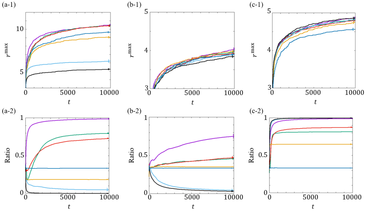
Figure 1: Transition plots of (x-1) the observed maximum and (x-2) the ratio of the optimal arm selection. (a) “Easy” problem, (b) “difficult” problem, and (c) “unfavorable” problem. The colors represent the following: purple, this work; green, ThresholdAscent; red, RobustUCBMax; sky blue, spUCB; orange, UCBE; black, conventional UCB; and blue, random search. The error bars indicate the standard errors of 100 independent runs. If the differences between the two methods are more than two times the standard errors, there will be a significant difference between these methods with a 5 % significance level.

6.2 Molecular discovery using tree search

As a demonstration of the molecular discovery problem, we attempted to optimize the molecular structure $M$ which maximized either of the properties defined by the following empirical equations (Joback and Reid, 1987):

$$T_{\text{b}}(M)\text{[K]}=198.2+\sum_{i\in\text{frag}(M)}T_{\text{b},i},$$

$$P_{\text{c}}(M)\text{[bar]}=\left[0.113+0.0032N_{\text{a}}(M)+\sum_{i\in\text{frag}(M)}P_{\text{c},i}\right]^{-2},$$

$$\eta_{300\text{K}}(M)\text{[Pa$\cdot$s]}=M_{\text{w}}(M)\exp{\left[\frac{\sum_{i\in\text{frag}(M)}\eta_{\text{a},i}-597.82}{300}+\sum_{i\in\text{frag}(M)}\eta_{\text{b},i}-11.202\right]},$$

where $T_{\text{b}}$, $P_{\text{c}}$, and $\eta_{300\text{K}}$ are the boiling temperature, critical pressure, and liquid dynamic viscosity at $300$ K of molecule $M$, respectively; $\text{frag}(M)$ was a set of atomic fragments of $M$, determined by Joback and Raid. The fragments simply determined for each atom type, such as carbon in methyl group, halogens, and ether oxygen in a ring group, etc. The functions $N_{\text{a}}(M)$ and $M_{\text{w}}(M)$ were the number of atoms in $M$ and molecular weight of $M$, respectively. The empirical parameters, $T_{\text{b},i}$, $P_{\text{c},i}$, $\eta_{\text{a},i}$, and $\eta_{\text{b},i}$, were optimized to reproduce the experimental properties. The properties, $T_{\text{b}}$, $P_{\text{c}}$, and $\eta_{300\text{K}}$, depended on the molecular structure through these parameters. In addition to those three properties, the topological polar surface area $\text{TPSA}(M)$ [$\text{\AA}^{2}$] ($\text{\AA}=0.1\text{nm}$) (Ertl et al., 2000) was maximized. Using these empirical formulas, we can verify the performance of the search algorithms in a short time.

During the search process, the candidate molecular structures were generated using the following context-free grammar (Hopcroft et al., 2001) of the SMILES strings (Weininger, 1988). Using the context-free grammar, we could create a simple maze game (Kikkawa et al., 2020) systematically. Here, we applied the following rules:

$$\begin{split}S&\rightarrow\text{C($X$)($Y$)($Y$)($Y$)},\text{C(=O)($Y$)($Y$)},\text{C($Y$)C($Y$)(=C($Y$)C($Y$))},{\rm or}\;\text{C(=O)(O($Y$))($Y$)},\\ X&\rightarrow\text{[H]},\text{F},\text{Cl},\text{Br},\text{C($X$)($Y$)($Y$)},\text{O($Y$)},\text{N($Y$)($Y$)},\text{C(=O)($Y$)},\\ \phantom{X}&\phantom{\rightarrow,,}\text{C($Y$)(=C($Y$)($Y$))},{\rm or}\;\text{C(=O)(O($Y$))},\\ Y&\rightarrow\text{[H]},\text{F},\text{Cl},\text{Br},\text{C($X$)($Y$)($Y$)},\text{C(=O)($Y$)},\text{C($Y$)(=C($Y$)($Y$))},{\rm or}\;\text{C(=O)(O($Y$))},\end{split}$$

where $S$, $X$, and $Y$ denote the non-terminal variables, and the upright characters denote the terminals. The start variable is set to $S$, and a string-generation process is completed when the string no longer has variables. The following additional rule was applied when the number of alphabets was greater than 40:

$$X\;{\rm or}\;Y\rightarrow\text{[H]}.$$

This rule guarantees the termination of the generation process within the moderate molecular size. This limit is approximately 500 g/mol in molecular weight, and most of the known molecules in the database are within the limit. We employed hydrogen as the termination atom, which is commonly used in organic chemistry. The alphabets include the explicit “H”, and exclude the parenthesis and equal symbols. The string “Br” and “Cl” are considered as two alphabets. The search space of this molecular generator contains significantly more than $6.248\times 10^{13}$ molecular species, which is the number of isomers in $\text{C}_{40}\text{H}_{82}$ (Yeh, 1995). We did not consider the synthesizability and the target scope of generated molecules; however, it can be considered by modifying the grammar in practical use.

The context-free language can be projected to a tree graph (Fig.2). Therefore, the molecular generator can be easily implemented with an MCTS algorithm, as shown in Algorithm 3. The node selection in each layer continues until a complete molecular string is created. Subsequently, the chemical property evaluation is performed, after which the property value is used as the reward. The reward value is recorded in each node passed in the creation, and it is used to calculate the selection indices in the next creation. The complete SMILES strings assigned on the different leaves are treated as the different molecules in this search algorithm even if these molecules have the same molecular symmetries.

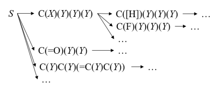
Figure 2: Tree image of SMILES generation.

Algorithm 3 MCTS

0:  number of trials $T$.

1:  $\tau=0$

2:  while $\tau<T$ do

3:     $\tau\leftarrow\tau+1$

4:     $v\leftarrow root()$ {the root node of the search tree.}

5:     $L\leftarrow\{v\}$

6:     while $v$ is not a leaf node do

7:        $k\leftarrow policy(records)${$policy$ : Algorithm 1 or the algorithms in Appendix B.$records$ : statistic data such as $K$, $n_{k}$, $R_{k}$, $R_{k}^{2}$, and $r^{\max}$ in Algorithm 1.}

8:        $L\leftarrow L\cup k$

9:        $v\leftarrow child(k,v)$ {the $k$-th child of the node $v$.}

10:     end while

11:     $r\leftarrow reward(L)$ {the reward of the selected path $L$.}

12:     $records.add(L,r)$ {record the path $L$ and the reward $r$.}

13:  end while

The properties, $T_{\text{b}}$, $P_{\text{c}}$, and $\eta_{300\text{K}}$ were calculated using the python thermo.joback module (Bell and Contributors, 2016), and TPSA was calculated using the RDKit library (Landrum, 2016). When using $\eta_{300\text{K}}$ as the reward, the rules containing one of F, N, and =C were excluded because their empirical parameters were not available. Additionally, we note that all of the generated SMILES were valid in the network test of RDKit.

Using the transition plots of the observed maximum, we compared MaxSearch and other algorithms in Figure 3. The plots of $T_{\text{b}}$, $P_{\text{c}}$, and TPSA were obtained by averaging over each 100 independent search runs. The plots of $\eta_{300\text{K}}$ were medians of the 100 runs with quantile error bars. Because of the large reward dispersion and skewness of $\eta_{300\text{K}}$, this treatment was required for the graph readability.

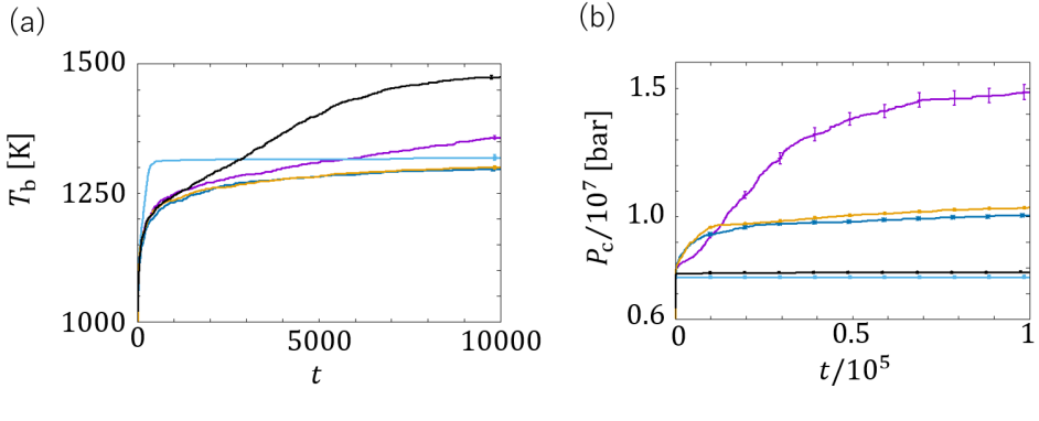
Figure 3: Transition plots of the molecular discovery. (a) $T_{\text{b}}$, (b) $P_{\text{c}}$, (c) $\eta_{300\text{K}}$, and (d) TPSA. The other notations are the same as those in Figure 1. The colors have the following representation: purple, this work; sky blue, spUCB; orange, UCBE; black, conventional UCB; and blue, random search. The error bars indicate the standard errors of the 100 independent runs in (a), (b), and (d). In (c), the quantiles are displayed instead of the standard errors. ThresholdAscent and RobustUCBMax cannot be implemented in MCTS because of the many hyperparameters involved.

In the search of $T_{\text{b}}$ in Fig. 3(a), the conventional UCB afforded the highest rewards at $t=10,000$. This result is expected because the empirical formula of $T_{\text{b}}$ is a simple sum of the fragment parameters. In such case, the optimal arm is almost equivalent to the arm with the best expectation reward. This condition corresponds to the “unfavorable” case of synthetic problems. In fact, the searches for other properties expressed by simple summation in the Joback method afforded similar results. For $t<2,500$, spUCB demonstrated the best performance. This result is probably due to the exploitative hyperparameters recommended in the original article (Schadd et al., 2008). The conventional UCB with a smaller $c$ gave a similar transition plot. Our algorithm exhibited the second-best performance in the late stage of the search process. The results of UCBE and the random search were worse than the above.

In the searches of $P_{\text{c}}$, $\eta_{300\text{K}}$, and TPSA, our algorithm demonstrated the best performance in the late stage. In the early stage of the search processes, UCBE exchibited better and highly stable performance. There are some different tendencies in these transition plots. These differences are probably due to the differences in the population distributions of rewards. For example, for $\eta_{300K}$, there are chemical structures with enormously high rewards in the search space. Our algorithm can find these structures with a high efficiency and success rate. In contrast, for TPSA, the population distribution probably has an upper bound near $290\text{ \AA}^{2}$. Even if such case, our algorithm worked well. These results evidence the wide application range of our proposed algorithm.

Samples of chemical structures with the highest $T_{b}$, $P_{c}$, $\eta_{300\text{K}}$, or TPSA of each run are shown in Figure 4. We have some understandings for high score molecules:

• Carboxyl groups are favorable for high $T_{b}$.

• Alcohol, carboxyl, and halogen groups are favorable for high viscosity.

• Polarized oxygen groups are favorable for high TPSA.

These understandings are consistent with chemical knowledge. More complicated and highly optimized structures can be found in our algorithm than in other algorithms.

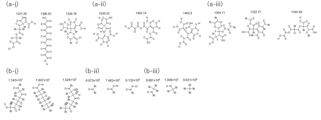
Figure 4: Sample of the chemical structures with the highest properties of each run. (a) $T_{b}$, (b) $P_{c}$, (c) $\eta_{300\text{K}}$, and (d) TPSA. (i) This work, (ii) UCB, and (iii) random search.

7 Discussion

The numerical experiments in the previous section show that a UCB of EI is suitable for the selection index for the MKB problem. In this section, we discuss why that is so. Our discussion would contain nonlogical arguments. However, we believe that this discussion will help with future work.

7.1 Subtleties of Extreme Regret

For our discussion, we should mention the subtleties of extreme regret, first pointed out by Nishihara et al. (2016). In this section, we review these subtleties.

The extreme regret was introduced by Carpentier and Valko (2014), defined as follows:

Definition 20 (Carpentier’s Regret)

In the MKB problem, Carpentier’s regret when $k(t),t\in[T]$ are selected is defined as follows:

$$R^{k_{*}(t),k(t)}_{\text{C}}(T)\coloneqq\mathbb{E}\left[\max_{t\in[T]}r_{k_{*}(t)}(t)\right]-\mathbb{E}\left[\max_{t\in[T]}r_{k(t)}(t)\right],$$ (30)

where $k_{*}(t),t\in[T]$ denotes an oracle policy. The asymptotically optimal policy should satisfy

$$R^{k_{*}(t),k(t)}_{\text{C}}(T)=o\left(\mathbb{E}\left[\max_{t\in[T]}r_{k_{*}(t)}(t)\right]\right).$$ (31)

A subtlety of Carpentier’s regret is that the regret asymptotically approaches $0$ for most policies in some settings. For example, we consider all reward distributions of the arms have bounded support. Then, any policy that selects each arm infinitely often achieves an asymtotically zero regret, meaning that even the random search is asymptotically optimal in the setting. It is a serious problem in previously proposed MKB algorithms because most of them are essentially based on Carpentier’s regret.

The problem of Carpentier’s regret means that this regret is unsuitable as an indicator of the asymptotically optimal policy. To avoid this, Nishihara et al. (2016) defined an alternative regret:

Definition 21 (Nishihara’s Regret)

In the MKB problem, Nishihara’s regret when $k(t),t\in[T^{\prime}]$ are selected is defined as follows:

$$R^{k_{*}(t),k(t)}_{\text{N}}(T)\coloneqq\frac{1}{T}\min_{T^{\prime}\geq 1}\left\{T^{\prime}:\mathbb{E}\left[\max_{t\in[T^{\prime}]}r_{k(t)}(t)\right]\geq\mathbb{E}\left[\max_{t\in[T]}r_{k_{*}(t)}(t)\right]\right\},$$ (32)

where $k_{*}(t),t\in[T]$ denotes an oracle policy. The asymptotically optimal policy should satisfy

$$\limsup_{T\to\infty}R^{k_{*}(t),k(t)}_{\text{N}}(T)\leq 1.$$ (33)

This regret works even when the reward distributions have finite supports. However, Nishihara et al. (2016) showed that there is a set of reward distributions such that

$$\limsup_{T\to\infty}R^{k_{*}^{\text{SA}},k(t)}_{\text{N}}(T)\geq K$$

for any policy, where $k_{*}^{\text{SA}}$ is the selection of single-armed oracle defined in Definition 22. Namely, no policy is asymptotically optimal under Nishihara’s regret.

Another subtlety exists in the definition of the oracle policy. The previous works are essentially based on the single-armed oracle (Nishihara et al., 2016) as follows:

Definition 22 (Single-Armed Oracle)

In the MKB problem, the single-armed oracle is the policy that plays the single arm

$$k_{*}^{\text{SA}}:={\mathop{\rm argmax}\limits}_{k\in[K]}\mathbb{E}\left[\max_{t\in[T]}r_{k}(t)\right]$$ (34)

over a time horizon $T$.

However, this oracle gives different $k_{*}^{\text{SA}}$ depending on $T$. This fact can be confirmed by the following example.

Example 1

Consider the MKB problem with $K=3$. Let the reward distributions of each arm be $f_{1}(r)=\mathcal{N}(r;0,0.01)$, $f_{2}(r)=\mathcal{N}(r;-1,0.25)$, $f_{3}(r)=\mathcal{N}(r;-15,4)$. Then, the single-armed oracle gives $k_{*}^{\text{SA}}=1$ if $T\leq 11$, $k_{*}^{\text{SA}}=2$ if $1.4\times 10^{11}\leq T\leq 5.4\times 10^{13}$, and $k_{*}^{\text{SA}}=3$ if $T\geq 3.9\times 10^{202}$.

Proof  The expected maximum reward sampled from the $k$-th arm over a time horizon $T$ is bounded by

$$\mu_{k}+\frac{1}{\sqrt{\pi\ln 2}}\sigma_{k}\sqrt{\ln T}\leq\mathbb{E}\left[\max_{t\in[T]}r_{k}(t)\right]\leq\mu_{k}+\sqrt{2}\sigma_{k}\sqrt{\ln T},$$ (35)

where $\mu_{k}$ and $\sigma^{2}_{k}$ are the mean and variance of the Gaussian reward distribution, $f_{k}(r)$, respectively (Kamath, 2015). Then, the example is established.  
The $T$-dependency of the single-armed oracle means that the best arm cannot be determined without information on $T$ (Nishihara et al., 2016). This raises a question about the regret analysis using the infinity limit of $T$. In Example 1, arm $3$ should be selected most often to achieve the asymptotically zero regret. However, arm $1$ or $2$ is a more suitable choice when $T<5.4\times 10^{13}$. Because many applications cannot perform such a large number of trials, the regret analysis result is impractical. The $T$-dependency of the oracle is also seriously inconvenient in MCTS applications. In an MCTS algorithm, $T$ is not given except for the root node. Then, one cannot determine the best arm except for the root node even if the reward distribution is known.

7.2 $T$-independent oracles and asymptotics of UCB approach

An oracle independent of $T$ was also proposed by Nishihara et al. (2016).

Definition 23 (Nishihara’s Greedy Oracle)

In the MKB problem, Nishihara’s greedy oracle is the policy that plays the arm with the maximum EI. Namely, this oracle plays

$$k_{*}^{\text{N}}(\tau):=\mathop{\rm argmax}\limits_{k\in[K]}\mathbb{E}\left[\max\left\{r_{k}(\tau),r_{*}^{\text{max}}(\tau-1)\right\}-r_{*}^{\text{max}}(\tau-1)|\{r_{k_{*}^{\text{N}}(t)}(t)\}_{t\in\tau-1}\right]$$ (36)

at time $\tau$, where $r_{*}^{\text{max}}(\tau)\coloneqq\max_{t\in[\tau]}r_{k_{*}^{\text{N}}}(t)$.

This oracle uses EI to avoid the dependency on $T$. Therefore, in terms of Nishihara’s greedy oracle, it is natural that we employ EI to derive a $T$-independent MKB algorithm. Although Nishihara et al. (2016) did not analyze this oracle much, we note that Nishihara’s greedy oracle gives different $k_{*}^{\text{N}}(\tau)$ depending on the oracle value $r_{*}^{\text{max}}(\tau)$ instead of $T$, as shown in the following example:

Example 2

Consider the MKB problem with $K=3$. Let the reward distributions of each arm be $f_{1}(r)=\mathcal{N}(r;0,1)$, $f_{2}(r)=\mathcal{N}(r;-2,2)$, $f_{3}(r)=\mathcal{N}(r;-6,3)$. Then, Nishihara’s greedy oracle gives $k_{*}^{\text{N}}(\tau)=1$ if $r_{*}^{\text{max}}(\tau-1)\leq 1.3$, $k_{*}^{\text{N}}(\tau)=2$ if $7.0\leq r_{*}^{\text{max}}(\tau-1)\leq 11.9$, and $k_{*}^{\text{N}}(\tau)=3$ if $r_{*}^{\text{max}}(\tau-1)\geq 18.9$,

Proof  Because of Lemma 12, we should consider the integral of the survival function. The survival function of $f_{k}(r)=\mathcal{N}(r;\mu_{k},\sigma_{k}^{2})$ is expressed as follows:

$$S(r)\coloneqq\int_{r}^{\infty}f_{k}(u)du=\frac{1}{2}~{}{\rm erfc}\left[\frac{r-\mu_{k}}{2\sigma_{k}}\right]$$ (37)

The bounds of $~{}{\rm erfc}(x),x>0$ are given by

$$c\exp(-\beta x^{2})<~{}{\rm erfc}(x)<\exp(-x^{2}),$$ (38)

where

$$c=\sqrt{\frac{2e}{\pi}}\frac{\sqrt{\beta-1}}{\beta},$$ (39)

and $\beta>1$ (Chiani et al., 2003; Chang et al., 2011). Then,

$$\frac{c}{2}\int_{y}^{\infty}\exp(-\beta x^{2})dx<\frac{1}{2}\int_{y}^{\infty}~{}{\rm erfc}(x)dx<\frac{1}{2}\int_{y}^{\infty}\exp(-x^{2})dx,$$ (40)

where $y>0$. Using the definition and bounds of $~{}{\rm erfc}(x)$ again, we obtain

$$\frac{\sqrt{\pi}c^{2}}{4\sqrt{\beta}}\exp(-\beta^{2}y^{2})<\frac{1}{2}\int_{y}^{\infty}~{}{\rm erfc}(x)dx<\frac{\sqrt{\pi}}{4}\exp(-y^{2}).$$ (41)

These bounds give the example.  
This dependency generates a subtlety in an adaptive case. Consider one obtains $r^{\text{max}}(\tau)<11.9$ under a selections $\{k(t)\}_{t\in[\tau]}$ in Example 2. A problem arises when the oracle value $r_{*}^{\text{max}}(\tau)>18.9$ at that time. In this case, the next selection of Nishihara’s greedy oracle differs from the selection with the maximum EI, meaning that a policy simply approaching Nishihara’s greedy oracle is not always effective in the MKB problem.

The subtlety due to the dependence on the oracle value $r_{*}^{\text{max}}(\tau)$ is solved using the observed value $r^{\text{max}}(\tau)$ alternatively. we define this oracle as follows:

Definition 24 (Kikkawa’s Greedy Oracle)

In the MKB problem, let $k(t),t\in[\tau-1]$ be the previous selections. Then, Kikkawa’s greedy oracle plays

$$k_{*}^{\text{K}}(\tau):=\mathop{\rm argmax}\limits_{k\in[K]}\mathbb{E}\left[\max\left\{r_{k}(\tau),r^{\text{max}}(\tau-1)\right\}-r^{\text{max}}(\tau-1)|\{r_{k(t)}(t)\}_{t\in\tau-1}\right]$$ (42)

at time $\tau$, where $r^{\text{max}}(\tau)\coloneqq\max_{t\in[\tau]}r_{k(t)}(t)$.

This oracle is equivalent to Nishihara’s greedy oracle when all selections follow this oracle. In addition, this oracle gives the arm that has the maximum EI even when the non-oracle selections exist in $k(t),t\in[\tau-1]$. The following proposition states that Kikkawa’s greedy oracle asymptotically approaches Nishihara’s greedy oracle in terms of Carpentier’s regret.

Proposition 25 (Asymptotics of Kikkawa’s Greedy Oracle)

Let $k(t),t\in[T]$ contain $o(T)$ non-oracle selections and other selections follow Kikkawa’s greedy oracle. Then,

$$R^{k_{*}^{N}(t),k(t)}_{\text{C}}(T)=o\left(\mathbb{E}\left[\max_{t\in[T]}r_{k_{*}^{N}(t)}(t)\right]\right),$$ (43)

when

$$\mathbb{E}\left[\max_{t\in[T]}r_{k_{*}^{N}(t)}(t)\right]\geq O(1)\ \text{and}\ EI\left[k,T;G^{\text{max}}\right]\leq O(T^{-1}).$$ (44)

Proof  Let $n_{k}(T),k\in[K]$ and $n_{k}^{\text{N}}(T),k\in[K]$ be the numbers of the $k$-th arm selected in $k(t),t\in[T]$ and $k_{*}^{\text{N}}(t),t\in[T]$, respectively. Then, $\delta n\coloneqq\left|n_{k}^{\text{N}}(T)-n_{k}(T)\right|=o(T)$ is expected. Therefore,

$$\begin{split}\left|R^{k_{*}^{\text{N}}(t),k(t)}_{\text{C}}(T)\right|&=\left|\mathbb{E}\left[\max_{k\in[K]}\max_{n\in[n_{k}^{\text{N}}(T)]}r_{k}(n)\right]-\mathbb{E}\left[\max_{k\in[K]}\max_{n\in[n_{k}(T)]}r_{k}(n)\right]\right|\\ &=\left|\mathbb{E}\left[\max_{k\in[K]}\left[\max\left\{\max_{n\in[n^{\text{min}}]}r_{k}(n),\max_{n\in[\delta n]}r_{k}(n+n^{\text{min}})\right\}-\max_{n\in[n^{\text{min}}]}r_{k}(n)\right]\right]\right|\\ &\leq\sum_{k\in[K]}\left|\mathbb{E}\left[\max\left\{\max_{n\in[n^{\text{min}}]}r_{k}(n),\max_{n\in[o(T)]}r_{k}(n+n^{\text{min}})\right\}-\max_{n\in[n^{\text{min}}]}r_{k}(n)\right]\right|\\ &\leq\sum_{k\in[K]}\left|o(T)EI\left[k,n^{\text{min}};G^{\text{max}}\right]\right|=o(1)\leq O\left(\mathbb{E}\left[\max_{t\in[T]}r_{k_{*}^{\text{N}}(t)}(t)\right]\right),\end{split}$$ (45)

where $n^{\text{min}}\coloneqq\min\{n_{k}^{\text{N}}(T),n_{k}(T)\}$.  
The proposition states that $o(T)$ mistakes are allowed in the asymptotically optimal policy under the condition related to the maximum value. This condition can be satisfied by Gaussian distributions at least.

Our concept in Section 4 can be obtained by simply substituting the EI in Kikkawa’s greedy oracle into its UCB. Therefore, our conceptual algorithm is expected to approach Kikkawa’s greedy oracle for large $T$. The number of non-oracle selections in the algorithm can be estimated as follows:

Proposition 26 (Number of Non-Oracle Selections)

Consider the MKB problem. Let $\overline{EI}\left[k,\mathcal{R}(t-1);G^{\text{sum}}\right],t\in[T]$ be an estimator of $EI\left[k,t;G^{\text{max}}\right]$. Suppose a confidence interval between $EI\left[k,t;G^{\text{max}}\right]$ and $\overline{EI}\left[k,\mathcal{R}(t-1);G^{\text{sum}}\right]$ is known as

$$\left|EI\left[k,t;G^{\text{max}}\right]-\overline{EI}\left[k,\mathcal{R}(t-1);G^{\text{sum}}\right]\right|\leq C(k,\alpha(t),n_{k}(t)),$$ (46)

with confidence level $1-\alpha(t)$, where $n_{k}(t),k\in[K]$ be the numbers of the $k$-th arm selected under Algorithm 1 with this confidence interval. Then, the number of non-oracle selections becomes $o(T)$ when $\alpha(t)=o(1)$ and $C(k,\alpha(t),n_{k}(t))=o(\{t/n_{k}(t)\}^{d})$ where $d>0$.

Proof  Consider the following events:

$$\begin{split}&A_{k_{*}^{\text{K}}(t),t}:\\ &\ \ \overline{EI}\left[k_{*}^{\text{K}}(t),\mathcal{R}(t-1);G^{\text{sum}}\right]\geq EI\left[k_{*}^{\text{K}}(t),t;G^{\text{max}}\right]-C\left(k_{*}^{\text{K}}(t),\alpha(t),n_{k_{*}^{\text{K}}(t)}(t)\right).\end{split}$$ (47)

$$A_{\kappa(t),t}:\overline{EI}\left[\kappa(t),\mathcal{R}(t-1);G^{\text{sum}}\right]\leq EI\left[\kappa(t),t;G^{\text{max}}\right]+C\left(\kappa(t),\alpha(t),n_{\kappa(t)}(t)\right),$$ (48)

where $\kappa(t)\in[K]/k_{*}^{\text{K}}(t)$. Then, the number of complementary cases can easily be counted as follows:

$$\sum_{t\in[T]}\mathbb{E}\left[\mathbbm{1}\left[\bigcup_{k\in[K]}A_{k,t}^{c}\right]\right]\leq K\sum_{t\in[T]}\alpha(t)=o(T).$$ (49)

Conversely, in the case of all $A_{k,t}$ established, the non-oracle arm is selected when

$$\begin{split}\overline{EI}\left[\kappa(t),\mathcal{R}(t-1);G^{\text{sum}}\right]&+C\left(\kappa(t),\alpha(t),n_{\kappa(t)}(t)\right)\\ &\geq\overline{EI}\left[k_{*}^{\text{K}}(t),\mathcal{R}(t-1);G^{\text{sum}}\right]+C\left(k_{*}^{\text{K}}(t),\alpha(t),n_{\kappa(t)}(t)\right),\end{split}$$ (50)

for any $\kappa(t)$. Then,

$$\begin{split}EI\left[k_{*}^{\text{K}}(t),t;G^{\text{max}}\right]&\leq\overline{EI}\left[k_{*}^{\text{K}}(t),\mathcal{R}(t-1);G^{\text{sum}}\right]+C(k_{*}^{\text{AG}}(t),\alpha(t),n_{k_{*}^{\text{K}}(t)}(t))\\ &\leq\overline{EI}\left[\kappa(t),\mathcal{R}(t-1);G^{\text{sum}}\right]+C(\kappa(t),\alpha(t),n_{\kappa(t)}(t))\\ &\leq EI\left[\kappa(t),t;G^{\text{max}}\right]+2C(\kappa(t),\alpha(t),n_{\kappa(t)}(t)).\end{split}$$ (51)

Equations (47), (48), and (50) are used in the first, second, and third inequalities, respectively. Then, solving for $n_{\kappa(t)}(t)$ using $C(k,\alpha(t),n_{\kappa(t)}(t))=o(\{t/n_{k}(t)\}^{d})$, we obtain

$$n_{\kappa(t)}(t)\leq 2^{1/d}\Delta_{\kappa(t)}(t)^{-1/d}o(t),$$ (52)

where

$$\Delta_{k}(t)=EI\left[k_{*}^{\text{K}}(t),t;G^{\text{max}}\right]-EI\left[k,t;G^{\text{max}}\right].$$ (53)

Using Equations (49) and (52), we obtain the proposition.  
This proposition means that Algorithm 1 asymptotically approaches Kikkawa’s greedy oracle in terms of the number of non-oracle selections. Considering Proposition 25, Algorithm 1 is also an asymptotically optimal policy in terms of Nishihara’s greedy oracle and Carpentier’s regret.

Notably, the proof of Proposition 26 is an analog of the proof for the conventional bandit problem (Auer et al., 2002; Jamieson, 2018) except for the optimal arm depending on the time $t$. This treatment can be allowed because the selections by Kikkawa’s greedy oracle correspond to the arms with the maximum EI for any $t$. This feature of Kikkawa’s greedy oracle is strong. We are sure that several other proofs for the conventional bandit problem will be established formally in the MKB problem using Kikkawa’s greedy oracle.

8 Conclusion

Here, we proposed an MKB algorithm and applied it to synthetic problems and molecular-design demonstrations using MCTS for materials discovery. The proposed algorithm only uses one hyperparameter and is easy to implement for MCTS. This feature gives the proposed algorithm an advantage over other MKB algorithms (Carpentier and Valko, 2014; David and Shimkin, 2016; Streeter and Smith, 2006b; Achab et al., 2017; Streeter and Smith, 2006a), and enables its application for materials discovery. In fact, to the best of our knowledge, this is the first case where the MKB algorithm is actually employed for materials discovery. The performance of the proposed algorithm was examined using the synthetic problems and the molecular-structure optimizations. The experimental results demonstrated that the proposed algorithm found the maximum reward more efficiently than other algorithms when the optimal arm could not be determined only based on the expectation reward. In real molecular designs, most of the molecular properties would have a high complexity; thus, we believe that the proposed algorithm is useful for these tasks.

In the theoretical aspect, we mainly contribute in two aspects. One is the proof of the effectiveness of the use of a UCB of EI. The proof result has wide flexibility and using this, other algorithms can be proposed with other assumptions for variables, which will be addressed in future work. The other is the proposal of Kikkawa’s greedy oracle. Using the proposed oracle, we can avoid many of the subtleties of the MKB problem.

Although we do not treat in this study, heuristics to reduce the required trials are also important for actual use. For example, the combination of the algorithm with UCBE may present a strategy for reducing the required trials. In addition, a combination with a supervised learning approach holds significant promise. The application of the proposed algorithm and the derivation into other areas are also important aspects that require further investigation.

Acknowledgments

We wish to thank Dr. Ryosuke Jinnouchi in TCRDL for reviewing our early draft.

Appendix A Proof of Theorem 17

Let $X_{i}$ be independent random variables drawn from the same sub-exponential $g(X)$ with parameter $b>0$. Then,

$$\begin{split}&\mathbb{P}\left\{\left|\frac{1}{n}\sum_{i=1}^{n}X_{i}-\mathbb{E}_{g(X)}\left[X\right]\right|\geq u\right\}\\ &=\mathbb{P}\left\{\frac{1}{n}\sum_{i=1}^{n}X_{i}-\mathbb{E}_{g(X)}\geq u\;\text{or}\;\mathbb{E}_{g(X)}-\mathbb{P}\left\{\frac{1}{n}\sum_{i=1}^{n}X_{i}\right\}\geq u\right\},\end{split}$$ (54)

where $u>0$. Therefore, in the former case,

$$\begin{split}&\mathbb{P}\left\{\frac{1}{n}\sum_{i=1}^{n}X_{i}-\mathbb{E}_{g(X)}\left[X\right]\geq u\right\}\\ &=\mathbb{P}\left\{\exp{\left(\frac{\lambda}{n}\sum_{i=1}^{n}X_{i}\right)}\geq\exp{\left[\lambda(u+\mathbb{E}_{g(X)}\left[X\right])\right]}\right\}\\ &\leq\exp{\left[-\lambda(u+\mathbb{E}_{g(X)}\left[X\right])\right]}\mathbb{E}\left[\exp{\left(\frac{\lambda}{n}\sum_{i=1}^{n}X_{i}\right)}\right],\;\;\;\langle{\rm Markov^{\prime}s}\;{\rm inequality}\rangle\end{split}$$ (55)

where $\lambda>0$ is an arbitrary parameter. Since the random variables $X_{i}$ are independent of each other, their moment-generating function can be separated. Thus, we obtain

$$\begin{split}&\mathbb{P}\left\{\frac{1}{n}\sum_{i=1}^{n}X_{i}-\mathbb{E}_{g(X)}\left[X\right]\geq u\right\}\\ &\leq\exp{\left[-\lambda(u+\mathbb{E}_{g(X)}\left[X\right])\right]}\left\{\mathbb{E}_{g(X)}\left[\exp{\left(\frac{\lambda X}{n}\right)}\right]\right\}^{n}\\ &=\exp{\left[-\lambda(u+\mathbb{E}_{g(X)}\left[X\right])\right]}\left(1+\frac{\lambda\mathbb{E}_{g(X)}\left[X\right]}{n}+\sum_{p=2}^{\infty}\frac{\lambda^{p}\mathbb{E}_{g(X)}\left[X^{p}\right]}{n^{p}p!}\right)^{n}\\ &\leq\exp{\left[-\lambda u+\sum_{p=2}^{\infty}\frac{\lambda^{p}\mathbb{E}_{g(X)}\left[X^{p}\right]}{n^{p-1}p!}\right]}\;\;\;\langle{\rm Since}\,1+x\leq\exp{x}\rangle\\ &=\exp{\left[-\lambda u+\sum_{p=2}^{\infty}\frac{\lambda^{p}}{n^{p-1}p!}\int_{0}^{\infty}\mathbb{P}_{g(X)}\{X^{p}\geq u\}\;du\right]}\;\;\;\langle{\rm Integral}\;{\rm identity}\rangle\\ &=\exp{\left[-\lambda u+\sum_{p=2}^{\infty}\frac{\lambda^{p}}{n^{p-1}p!}\int_{0}^{\infty}\mathbb{P}_{g(X)}\{X\geq bv\}pb^{p}v^{p-1}\;dv\right]}\;\;\;\langle{\rm Replace}\;u\;{\rm with}\;b^{p}v^{p}\rangle\\ &\leq\exp{\left[-\lambda u+2\sum_{p=2}^{\infty}\frac{\lambda^{p}b^{p}}{n^{p-1}(p-1)!}\int_{0}^{\infty}e^{-v}v^{p-1}\;dv\right]}.\;\;\;\langle{\rm Sub\mathchar 45\relax exponential}\rangle\end{split}$$ (56)

The above integral corresponds to the Gamma function. Therefore,

$$\begin{split}\mathbb{P}\left\{\frac{1}{n}\sum_{i=1}^{n}X_{i}-\mathbb{E}_{g(X)}\left[X\right]\geq u\right\}&\leq\exp{\left[-\lambda u+2\sum_{p=2}^{\infty}\frac{b^{p}\lambda^{p}\Gamma(p)}{n^{p-1}(p-1)!}\right]}\\ &=\exp{\left[-\lambda u+2\sum_{p=2}^{\infty}\frac{b^{p}\lambda^{p}}{n^{p-1}}\right]}\\ &=\exp{\left[-\lambda u+\frac{2b^{2}\lambda^{2}}{n-b\lambda}\right]},\end{split}$$ (57)

where $\left|b\lambda/n\right|<1$. Replacing $n-b\lambda$ with $\xi_{+}$, we obtain

$$\mathbb{P}\left\{\frac{1}{n}\sum_{i=1}^{n}X_{i}-\mathbb{E}_{g(X)}\left[X\right]\geq u\right\}\leq\exp{\left[\left(\frac{u}{b}+2\right)\xi_{+}+\frac{2n^{2}}{\xi_{+}}-\frac{nu}{b}-4n\right]},$$ (58)

where $0<\xi_{+}<2n$. Hence, the optimized $\xi_{+}$ is

$$\xi_{+}=\sqrt{\frac{2n^{2}b}{2b+u}}.$$ (59)

Then,

$$\mathbb{P}\left\{\frac{1}{n}\sum_{i=1}^{n}X_{i}-\mathbb{E}_{g(X)}\left[X\right]\geq u\right\}\leq\exp{\left(2\sqrt{2}nw_{+}-nw_{+}^{2}-2n\right)},$$ (60)

where $w_{+}\coloneqq\sqrt{ub^{-1}+2}\geq\sqrt{2}$. Moreover, using the same approach, we obtain

$$\mathbb{P}\left\{\mathbb{E}_{g(X)}\left[X\right]-\frac{1}{n}\sum_{i=1}^{n}X_{i}\geq u\right\}\leq\exp{\left[\left(-\frac{u}{b}+2\right)\xi_{-}+\frac{2n^{2}}{\xi_{-}}+\frac{nu}{b}-4n\right]},$$ (61)

where $\xi_{-}\coloneqq n+b\lambda$ and $0<\xi_{-}<2n$. Hence, the optimized $\xi_{-}$ is

$$\xi_{-}=\left\{\begin{array}[]{ll}\sqrt{2n^{2}b/(2b-u)}&0\leq u<3b/2\\ 2n-\epsilon&3b/2\leq u,\end{array}\right.$$ (62)

where $\epsilon$ is an infinitesimal. Then, we obtain

$$\mathbb{P}\left\{\mathbb{E}_{g(X)}\left[X\right]-\frac{1}{n}\sum_{i=1}^{n}X_{i}\geq u\right\}\leq\left\{\begin{array}[]{ll}\exp{(2\sqrt{2}nw_{-}-nw_{-}^{2}-2n)}&0\leq u<3b/2\\ \exp{\left[\left(-ub^{-1}+1\right)n+O(\epsilon)\right]}&3b/2\leq u,\end{array}\right.$$ (63)

where $w_{-}\coloneqq\sqrt{-ub^{-1}+2}>1/\sqrt{2}$. Equations 60 and 63 show that $\mathbb{E}\left[X\right]$ is bounded at a confidence level of $1-\alpha>0$ as follows:

$$\frac{1}{n}\sum_{i=1}^{n}X_{i}-u_{+}^{*}\leq\mathbb{E}\left[X\right]\leq\frac{1}{n}\sum_{i=1}^{n}X_{i}+u_{-}^{*},$$ (64)

where

$$\alpha=\exp{\left[2\sqrt{2}nw_{+}^{*}-n(w_{+}^{*})^{2}-2n\right]},$$ (65)

when $u_{+}^{*}\geq 0$, and

$$\alpha=\left\{\begin{array}[]{ll}\exp{\left[2\sqrt{2}nw_{-}^{*}-n(w_{-}^{*})^{2}-2n\right]}&0\leq u_{-}^{*}<3b/2\\ \exp{\left[\left(-u_{-}^{*}b^{-1}+1\right)n\right]}&3b/2\leq u_{-}^{*},\end{array}\right.$$ (66)

where $w_{\pm}^{*}\coloneqq\sqrt{\pm u_{\pm}^{*}b^{-1}+2}$ (double sign in the same order). From Eq. 65, we obtain

$$w_{+}^{*}=\sqrt{2}+\beta,$$ (67)

and

$$u_{+}^{*}=(\beta^{2}+2\sqrt{2}\beta)b,$$ (68)

where $\beta\coloneqq\sqrt{-\ln\alpha/n}$. In addition, from Eq. 66,

$$u_{-}^{*}=\left\{\begin{array}[]{ll}(-\beta^{2}+2\sqrt{2}\beta)b&0\leq\beta<1/\sqrt{2}\\ (\beta^{2}+1)b&1/\sqrt{2}\leq\beta.\end{array}\right.$$ (69)

The theorem follows from Eqs. 60 and 63.

Appendix B Compared Algorithms

We compared our algorithm with Algorithms 4-9. We employed the following hyperparameters and applied some modifications for the implementation. In ThresholdAscent, the hyper-parameters were set to $s=100$ and $\delta=2\ln\nu$. We used the reward ranking instead of the iteration used in the original code (Streeter and Smith, 2006b). In RobustUCBMax, we set $u=r^{100\text{-th}}$, $v=(r^{\max}-u)^{1+\epsilon}$, and $\epsilon=0.4$, according to the original paper (Achab et al., 2017). Although the original paper employed the robust UCB with the truncated mean estimator, we used a simple version of the robust UCB (Bubeck et al., 2013). In spUCB, $c=0.1$ and $D=32$ are used as the hyper-parameters. These values are recommended in the original paper (Schadd et al., 2008). In UCBE (Audibert et al., 2010) and the conventional UCB (Auer et al., 2002), we used $c=1$ as the hyperparameter. In some algorithms, we estimated the variance parameter, $\sigma$, as the sample variance of the first $P=10$ random searches.

Algorithm 4 ThresholdAscent

0:  number of arms $K$, time horizon $T$, the $s$-th maximum of observed reward $r^{s\text{-th}}$ number of times the $k$-th arm is selected $n_{k}$, the $i$-th reward from the $k$-th arm $r_{k,i}$, and hyper-parameter $\delta$.

0:  selected arm index $\hat{k}$.

1:  for each $k\in[K]$ do

2:     if $n_{k}=0$ or $\nu<2$ then

3:        $z_{k}\leftarrow\infty$

4:     else

5:        $S_{k}=\sum_{i\in[n_{k}]}\mathbbm{1}[r_{k,i}>r^{s\text{-th}}]$

6:        $\alpha\leftarrow\ln(2TK/\delta)$

7:        $z_{k}\leftarrow S_{k}/n_{k}+(\alpha+\sqrt{\alpha(2S_{k}+\alpha)})/n_{k}$

8:     end if

9:  end for

10:  $\hat{k}\leftarrow\mathop{\rm argmax}\limits_{k\in[K]}z_{k}$

11:  return  $\hat{k}$

Algorithm 5 RobustUCBMax

0:  number of arms $K$, number of times the $k$-th arm is selected $n_{k}$, the $i$-th reward from the $k$-th arm $r_{k,i}$, and hyper-parameters $u$, $v$, and $\epsilon$.

0:  selected arm index $\hat{k}$.

1:  $\nu=\sum_{k\in[K]}n_{k}$

2:  for each $k\in[K]$ do

3:     if $n_{k}=0$ or $\nu<2$ then

4:        $z_{k}\leftarrow\infty$

5:     else

6:        $S_{k}=\sum_{i\in[n_{k}]}r_{k,i}\mathbbm{1}[r_{k,i}>u]$

7:        $z_{k}\leftarrow S_{k}/n_{k}\ +4v^{1/(1+\epsilon)}(2\ln\nu/n_{k})^{\epsilon/(1+\epsilon)}$

8:     end if

9:  end for

10:  $\hat{k}\leftarrow\mathop{\rm argmax}\limits_{k\in[K]}z_{k}$

11:  return  $\hat{k}$

Algorithm 6 spUCB

0:  number of arms $K$, current time $\tau$, number of times the $k$-th arm is selected $n_{k}$, sum of the rewards obtained from the $k$-th arm $R_{k}$, sum of square rewards obtained from the $k$-th arm $Q_{k}$, and sample variance obtained from the first $P$ trials $\sigma$.

0:  selected arm index $\hat{k}$.

1:  if $\tau\leq P$ then

2:     $\hat{k}\leftarrow RandomSearch(K)$

3:  else

4:     $\nu=\sum_{k\in[K]}n_{k}$

5:     for each $k\in[K]$ do

6:        if $n_{k}=0$ or $\nu<2$ then

7:           $z_{k}\leftarrow\infty$

8:        else

9:           $m_{k}\leftarrow R_{k}/n_{k}$

10:           $z_{k}\leftarrow m_{k}+c\sigma\sqrt{\ln\nu/n_{k}}\ +\sqrt{\frac{Q_{k}-n_{k}m_{k}^{2}+D}{n_{k}}}$

11:        end if

12:     end for

13:     $\hat{k}\leftarrow\mathop{\rm argmax}\limits_{k\in[K]}z_{k}$

14:  end if

15:  return  $\hat{k}$

Algorithm 7 UCBE

0:  number of arms $K$, current time $\tau$, number of times the $k$-th arm is selected $n_{k}$, sum of the rewards obtained from the $k$-th arm $R_{k}$, and sample variance obtained from the first $P$ trials $\sigma$.

0:  selected arm index $\hat{k}$.

1:  if $\tau\leq P$ then

2:     $\hat{k}\leftarrow RandomSearch(K)$

3:  else

4:     $\nu=\sum_{k\in[K]}n_{k}$

5:     for each $k\in[K]$ do

6:        if $n_{k}=0$ or $\nu<2$ then

7:           $z_{k}\leftarrow\infty$

8:        else

9:           $z_{k}\leftarrow R_{k}/n_{k}+c\sigma\sqrt{\nu/n_{k}}$

10:        end if

11:     end for

12:     $\hat{k}\leftarrow\mathop{\rm argmax}\limits_{k\in[K]}z_{k}$

13:  end if

14:  return  $\hat{k}$

Algorithm 8 UCB

0:  number of arms $K$, current time $\tau$, number of times the $k$-th arm is selected $n_{k}$, sum of the rewards obtained from the $k$-th arm $R_{k}$, and sample variance obtained from the first $P$ trials $\sigma$.

0:  selected arm index $\hat{k}$.

1:  if $\tau\leq P$ then

2:     $\hat{k}\leftarrow RandomSearch(K)$

3:  else

4:     $\nu=\sum_{k\in[K]}n_{k}$

5:     for each $k\in[K]$ do

6:        if $n_{k}=0$ or $\nu<2$ then

7:           $z_{k}\leftarrow\infty$

8:        else

9:           $z_{k}\leftarrow R_{k}/n_{k}+c\sigma\sqrt{\ln\nu/n_{k}}$

10:        end if

11:     end for

12:     $\hat{k}\leftarrow\mathop{\rm argmax}\limits_{k\in[K]}z_{k}$

13:  end if

14:  return  $\hat{k}$

Algorithm 9 RandomSearch

0:  number of arms $K$.

0:  selected arm index $\hat{k}$.

1:  $\hat{k}\leftarrow random(K)$ {randomly select any of $1,...,K$.}

2:  return  $\hat{k}$

References

- Achab et al. (2017) Mastane Achab, Stephan Clémençon, Aurélien Garivier, Anne Sabourin, and Claire Vernade. Max k-armed bandit: On the extremehunter algorithm and beyond. In Joint European Conference on Machine Learning and Knowledge Discovery in Databases, pages 389–404. Springer, 2017.
- Agrawal and Choudhary (2019) Ankit Agrawal and Alok Choudhary. Deep materials informatics: Applications of deep learning in materials science. MRS Communications, 9(3):779–792, 2019.
- Audibert et al. (2010) Jean-Yves Audibert, Sébastien Bubeck, and Rémi Munos. Best arm identification in multi-armed bandits. In COLT, pages 41–53. Citeseer, 2010.
- Auer et al. (2002) Peter Auer, Nicolo Cesa-Bianchi, and Paul Fischer. Finite-time analysis of the multiarmed bandit problem. Machine learning, 47(2):235–256, 2002.
- Bell and Contributors (2016) Caleb Bell and Contributors. Thermo: Chemical properties component of chemical engineering design library (chedl). 2016. URL https://github.com/CalebBell/thermo.
- Browne et al. (2012) Cameron B Browne, Edward Powley, Daniel Whitehouse, Simon M Lucas, Peter I Cowling, Philipp Rohlfshagen, Stephen Tavener, Diego Perez, Spyridon Samothrakis, and Simon Colton. A survey of monte carlo tree search methods. IEEE Transactions on Computational Intelligence and AI in games, 4(1):1–43, 2012.
- Bubeck et al. (2013) Sébastien Bubeck, Nicolo Cesa-Bianchi, and Gábor Lugosi. Bandits with heavy tail. IEEE Transactions on Information Theory, 59(11):7711–7717, 2013.
- Butler et al. (2018) Keith T Butler, Daniel W Davies, Hugh Cartwright, Olexandr Isayev, and Aron Walsh. Machine learning for molecular and materials science. Nature, 559(7715):547–555, 2018.
- Carpentier and Valko (2014) Alexandra Carpentier and Michal Valko. Extreme bandits. In Neural Information Processing Systems, 2014.
- Chang et al. (2011) Seok-Ho Chang, Pamela C Cosman, and Laurence B Milstein. Chernoff-type bounds for the gaussian error function. IEEE Transactions on Communications, 59(11):2939–2944, 2011.
- Chiani et al. (2003) Marco Chiani, Davide Dardari, and Marvin K Simon. New exponential bounds and approximations for the computation of error probability in fading channels. IEEE Transactions on Wireless Communications, 2(4):840–845, 2003.
- Cicirello and Smith (2005) Vincent A Cicirello and Stephen F Smith. The max k-armed bandit: A new model of exploration applied to search heuristic selection. In The Proceedings of the Twentieth National Conference on Artificial Intelligence, volume 3, pages 1355–1361, 2005.
- David and Shimkin (2016) Yahel David and Nahum Shimkin. PAC lower bounds and efficient algorithms for the max k-armed bandit problem. In International Conference on Machine Learning, pages 878–887. PMLR, 2016.
- Del Rosario et al. (2020) Zachary Del Rosario, Matthias Rupp, Yoolhee Kim, Erin Antono, and Julia Ling. Assessing the frontier: Active learning, model accuracy, and multi-objective candidate discovery and optimization. The Journal of Chemical Physics, 153(2):024112, 2020.
- Ertl et al. (2000) Peter Ertl, Bernhard Rohde, and Paul Selzer. Fast calculation of molecular polar surface area as a sum of fragment-based contributions and its application to the prediction of drug transport properties. Journal of Medicinal Chemistry, 43(20):3714–3717, Oct 2000. ISSN 0022-2623. doi: 10.1021/jm000942e. URL https://doi.org/10.1021/jm000942e.
- Hopcroft et al. (2001) John E. Hopcroft, Rajeev Motwani, and Jeffrey D. Ullman. Introduction to automata theory, languages, and computation, 2nd edition. SIGACT News, 32(1):60–65, March 2001. ISSN 0163-5700. doi: 10.1145/568438.568455. URL https://doi.org/10.1145/568438.568455.
- Jamieson (2018) Kevin Jamieson. Lecture 3: Stochastic multi-armed bandits, regret minimization, 2018. URL https://courses.cs.washington.edu/courses/cse599i/18wi/resources/lecture3/lecture3.pdf.
- Jha et al. (2018) Dipendra Jha, Logan Ward, Arindam Paul, Wei-keng Liao, Alok Choudhary, Chris Wolverton, and Ankit Agrawal. Elemnet: Deep learning the chemistry of materials from only elemental composition. Scientific reports, 8(1):1–13, 2018.
- Jha et al. (2019) Dipendra Jha, Kamal Choudhary, Francesca Tavazza, Wei-keng Liao, Alok Choudhary, Carelyn Campbell, and Ankit Agrawal. Enhancing materials property prediction by leveraging computational and experimental data using deep transfer learning. Nature communications, 10(1):1–12, 2019.
- Joback and Reid (1987) K. G. Joback and R. Reid. Estimation of pure-component properties from group-contributions. Chemical Engineering Communications, 57:233–243, 1987.
- Ju et al. (2018) Shenghong Ju, TM Dieb, K Tsuda, and J Shiomi. Optimizing interface/surface roughness for thermal transport. In Machine Learning for Molecules and Materials NIPS 2018 Workshop, 2018.
- Kajita et al. (2020) Seiji Kajita, Tomoyuki Kinjo, and Tomoki Nishi. Autonomous molecular design by Monte-Carlo tree search and rapid evaluations using molecular dynamics simulations. Communications Physics, 3(1):1–11, 2020.
- Kamath (2015) Gautam Kamath. Bounds on the expectation of the maximum of samples from a gaussian. URL http://www. gautamkamath. com/writings/gaussian max. pdf, 2015.
- Kikkawa et al. (2020) Nobuaki Kikkawa, Seiji Kajita, and Kensuke Takechi. Self-learning molecular design for high lithium-ion conductive ionic liquids using maze game. Journal of Chemical Information and Modeling, 60(10):4904–4911, 2020.
- Kiyohara and Mizoguchi (2018) Shin Kiyohara and Teruyasu Mizoguchi. Searching the stable segregation configuration at the grain boundary by a monte carlo tree search. The Journal of chemical physics, 148(24):241741, 2018.
- Kocsis and Szepesvári (2006) Levente Kocsis and Csaba Szepesvári. Bandit based monte-carlo planning. In European conference on machine learning, pages 282–293. Springer, 2006.
- Kusne et al. (2020) A Gilad Kusne, Heshan Yu, Changming Wu, Huairuo Zhang, Jason Hattrick-Simpers, Brian DeCost, Suchismita Sarker, Corey Oses, Cormac Toher, Stefano Curtarolo, et al. On-the-fly closed-loop materials discovery via Bayesian active learning. Nature communications, 11(1):1–11, 2020.
- Lai and Robbins (1985) Tze Leung Lai and Herbert Robbins. Asymptotically efficient adaptive allocation rules. Advances in applied mathematics, 6(1):4–22, 1985.
- Landrum (2016) Greg Landrum. RDKit: Open-source cheminformatics software. 2016. URL https://github.com/rdkit/rdkit/releases/tag/Release_2016_09_04.
- Liu et al. (2017) Yue Liu, Tianlu Zhao, Wangwei Ju, and Siqi Shi. Materials discovery and design using machine learning. Journal of Materiomics, 3(3):159–177, 2017. ISSN 2352-8478. doi: https://doi.org/10.1016/j.jmat.2017.08.002.
- M. Dieb et al. (2017) Thaer M. Dieb, Shenghong Ju, Kazuki Yoshizoe, Zhufeng Hou, Junichiro Shiomi, and Koji Tsuda. MDTS: automatic complex materials design using Monte Carlo tree search. Science and technology of advanced materials, 18(1):498–503, 2017.
- M. Dieb et al. (2018) Thaer M. Dieb, Zhufeng Hou, and Koji Tsuda. Structure prediction of boron-doped graphene by machine learning. The Journal of chemical physics, 148(24):241716, 2018.
- Meredig et al. (2018) Bryce Meredig, Erin Antono, Carena Church, Maxwell Hutchinson, Julia Ling, Sean Paradiso, Ben Blaiszik, Ian Foster, Brenna Gibbons, Jason Hattrick-Simpers, Apurva Mehta, and Logan Ward. Can machine learning identify the next high-temperature superconductor? examining extrapolation performance for materials discovery. Mol. Syst. Des. Eng., 3:819–825, 2018. doi: 10.1039/C8ME00012C.
- Nishihara et al. (2016) Robert Nishihara, David Lopez-Paz, and Léon Bottou. No regret bound for extreme bandits. In Artificial Intelligence and Statistics, pages 259–267. PMLR, 2016.
- Olivecrona et al. (2017) Marcus Olivecrona, Thomas Blaschke, Ola Engkvist, and Hongming Chen. Molecular de-novo design through deep reinforcement learning. Journal of cheminformatics, 9(1):1–14, 2017.
- Patra et al. (2020) Tarak K Patra, Troy D Loeffler, and Subramanian KRS Sankaranarayanan. Accelerating copolymer inverse design using monte carlo tree search. Nanoscale, 12(46):23653–23662, 2020.
- Pilania et al. (2013) Ghanshyam Pilania, Chenchen Wang, Xun Jiang, Sanguthevar Rajasekaran, and Ramamurthy Ramprasad. Accelerating materials property predictions using machine learning. Scientific reports, 3(1):1–6, 2013.
- Popova et al. (2018) Mariya Popova, Olexandr Isayev, and Alexander Tropsha. Deep reinforcement learning for de novo drug design. Science advances, 4(7):eaap7885, 2018.
- Raccuglia et al. (2016) Paul Raccuglia, Katherine C Elbert, Philip DF Adler, Casey Falk, Malia B Wenny, Aurelio Mollo, Matthias Zeller, Sorelle A Friedler, Joshua Schrier, and Alexander J Norquist. Machine-learning-assisted materials discovery using failed experiments. Nature, 533(7601):73–76, 2016.
- Ramprasad et al. (2017) Rampi Ramprasad, Rohit Batra, Ghanshyam Pilania, Arun Mannodi-Kanakkithodi, and Chiho Kim. Machine learning in materials informatics: recent applications and prospects. npj Computational Materials, 3(1):1–13, 2017.
- Sanchez-Lengeling and Aspuru-Guzik (2018) Benjamin Sanchez-Lengeling and Alán Aspuru-Guzik. Inverse molecular design using machine learning: Generative models for matter engineering. Science, 361(6400):360–365, 2018.
- Sanchez-Lengeling et al. (2017) Benjamin Sanchez-Lengeling, Carlos Outeiral, Gabriel L Guimaraes, and Alan Aspuru-Guzik. Optimizing distributions over molecular space. an objective-reinforced generative adversarial network for inverse-design chemistry (ORGANIC). ChemRxiv, 2017, 2017.
- Schadd et al. (2008) Maarten PD Schadd, Mark HM Winands, H Jaap Van Den Herik, Guillaume MJ-B Chaslot, and Jos WHM Uiterwijk. Single-player monte-carlo tree search. In International Conference on Computers and Games, pages 1–12. Springer, 2008.
- Segler et al. (2018) Marwin HS Segler, Mike Preuss, and Mark P Waller. Planning chemical syntheses with deep neural networks and symbolic AI. Nature, 555(7698):604–610, 2018.
- Streeter and Smith (2006a) Matthew J Streeter and Stephen F Smith. An asymptotically optimal algorithm for the max k-armed bandit problem. In AAAI, pages 135–142, 2006a.
- Streeter and Smith (2006b) Matthew J Streeter and Stephen F Smith. A simple distribution-free approach to the max k-armed bandit problem. In International Conference on Principles and Practice of Constraint Programming, pages 560–574. Springer, 2006b.
- Sutton and Barto (2018) Richard S Sutton and Andrew G Barto. Reinforcement learning: An introduction. MIT press, 2018.
- Ueno et al. (2016) Tsuyoshi Ueno, Trevor David Rhone, Zhufeng Hou, Teruyasu Mizoguchi, and Koji Tsuda. COMBO: an efficient Bayesian optimization library for materials science. Materials discovery, 4:18–21, 2016.
- Vershynin (2018) Roman Vershynin. High-dimensional probability: An introduction with applications in data science, volume 47. Cambridge university press, 2018.
- Weininger (1988) David Weininger. SMILES, a chemical language and information system. 1. introduction to methodology and encoding rules. Journal of Chemical Information and Computer Sciences, 28(1):31–36, Feb 1988. ISSN 0095-2338. doi: 10.1021/ci00057a005. URL https://pubs.acs.org/doi/abs/10.1021/ci00057a005.
- Yamada et al. (2019) Hironao Yamada, Chang Liu, Stephen Wu, Yukinori Koyama, Shenghong Ju, Junichiro Shiomi, Junko Morikawa, and Ryo Yoshida. Predicting materials properties with little data using shotgun transfer learning. ACS central science, 5(10):1717–1730, 2019.
- Yang et al. (2017) Xiufeng Yang, Jinzhe Zhang, Kazuki Yoshizoe, Kei Terayama, and Koji Tsuda. ChemTS: an efficient python library for de novo molecular generation. Science and technology of advanced materials, 18(1):972–976, 2017.
- Yeh (1995) Chin-yah Yeh. Isomer enumeration of alkanes, labeled alkanes, and monosubstituted alkanes. Journal of chemical information and computer sciences, 35(5):912–913, 1995.