Rationally Inattentive Statistical Discrimination: Arrow Meets Phelps

Abstract

When information acquisition is costly but flexible, a principal may rationally acquire information that favors “majorities” over “minorities.” Majorities therefore face incentives to invest in becoming productive, whereas minorities are discouraged from such investments. The principal, in turn, rationally ignores minorities unless they surprise him with a genuinely outstanding outcome, precisely because they are less likely to invest. We give conditions under which the resulting discriminatory equilibrium is most preferred by the principal, despite that all groups are ex-ante identical. Our results add to the discussions of affirmative action, implicit bias, and occupational segregation and stereotypes.

Keywords: Statistical discrimination; rational inattention; incentive contracting

JEL codes: D82, D86, D31, J71

1 Introduction

We provide a new account of statistical discrimination. A demographic group is discriminated against in the labor market because its members rationally choose to underinvest in the skills needed to succeed. Their investment choice is reinforced by the endogenous allocation of an employer’s limited attention across groups, based on which beliefs about the returns to investing are formed, and labor market decisions are made. In equilibrium, discriminatory attention allocation and differing investment choices between ex-ante identical groups are mutually reinforcing. Under some conditions, discriminatory equilibria are the most profitable to the employer.

The theory of statistical discrimination posits that groups of individuals with certain demographic traits are discriminated against in the labor market, because rational employers correctly infer that these groups should be treated differently. As an explanation for discrimination, the theory does not rely on bias or adversarial feelings towards discriminated groups, although both bias and rational beliefs may play a role in any given real-world instance of discrimination. A key element of the theory is the mechanism by which employers form discriminatory beliefs.

Economists have put forward two canonical models of statistical discrimination: the Arrovian model of coordination failure, and the Phelpsian model of information heterogeneity. Arrow (1971, 1998) argues that discrimination may arise as the result of coordination failure. One demographic collective, call it Group 1, expects to be discriminated against, and therefore does not undertake the costly investments that are needed to succeed in the labor market. Group 2 expects to be favored, and therefore finds it worthwhile to invest. Employers, in turn, rationally discriminate against Group 1 in favor of Group 2 because the latter is expected to invest and the former is not. Such a discriminatory equilibrium is, typically, Pareto dominated by an impartial equilibrium whereby employers hold uniformly positive beliefs about all groups, and the latter all invest.

The second canonical model follows Phelps (1972) (see also Aigner and Cain 1977) to argue that statistical discrimination emerges from differing qualities of information. Groups 1 and 2 have the same, exogenous, skill distribution, but employers have access to better-quality information about members of Group 2 than of Group 1. As a result, members of Group 2 enjoy, on average, a favorable treatment in the labor market. Beyond a few well-studied cases such as biases in testing methodology, shared language, cultural background, or social connections (Cornell and Welch, 1996), the reasons behind the informational heterogeneity are often left unspecified.

The current paper combines ideas from the canonical Arrovian and Phelpsian models, with the chief aim of endogenizing employer’s acquisition of information about workers’ skills. In our story, workers choose whether to undertake a costly investment that results in an increased likelihood of being productive. An employer chooses a labor market outcome (a promotion decision, in our model), based on his endogenously gleaned information about workers’ productivity. We borrow from the recent literature on rational inattention (Sims, 2003) to model how an employer chooses a costly signal structure that will inform him about workers’ productivity. In equilibrium, workers’ incentives to invest are affected by how they expect to be rewarded by the employer, a decision that is filtered through the endogenously chosen information structure. In turn, the employer chooses an optimal information structure and labor market outcome, given his belief about workers’ investment decisions.

We first demonstrate that there always exists an impartial equilibrium: analogous to the equilibria without coordination failure in Arrow’s model, but with the new feature that the information structure endogenously chosen by the employer is also impartial about groups. In an impartial equilibrium, there is neither Arrovian coordination failure nor Phelpsian information heterogeneity.

Our main results describe the emergence of a discriminatory equilibrium, one that is not impartial. In a discriminatory equilibrium, members of different groups face different incentives to undertake costly investments. Again, as in Arrow, some groups choose not to invest because they are not expected to, while others do invest, and correctly expect to be rewarded. In our model, however, workers’ differing investment decisions are mirrored in the employer’s choice of a discriminatory information structure — one that favors the group who chooses to invest, unless the underinvested group is strictly more productive than the former; Arrow meets Phelps. In this way, the employer can efficiently deploy his limited attentional resources according to workers’ investment decisions, focusing mainly on whether the underinvested group surprises him with a genuinely outstanding outcome. The resulting belief favors the invested group most of the time, and thus reinforces workers’ expectations that they will be treated differently; a vicious circle is closed.

The following diagram plots the model’s behavior against an attention cost parameter that captures how costly it is for the employer to acquire information:

Our model exhibits two regimes: one in which the only equilibrium is impartial, and one where an impartial equilibrium and a discriminatory equilibrium coexist. The impartial equilibrium features high worker investments when the attention cost parameter is low, and low investments when the attention cost is high. A discriminatory equilibrium emerges when the attention cost parameter is intermediate, and it constitutes the most profitable equilibrium to the employer when it coexists with an impartial equilibrium that induces low worker investments.

There are three basic takeaway messages from our main results. First, a discriminatory signal structure can emerge endogenously, when workers are ex-ante identical but nonetheless face different incentives to invest. The differential incentives between workers explains the use of a discriminatory signal structure by the employer, which in turn leads workers to invest differently in equilibrium.

Second, the discriminatory equilibrium may be strictly preferred by the employer to an impartial equilibrium (in contrast with the baseline Arrovian model where discrimination is Pareto-dominated by the impartial equilibrium). The reason is that, when the attention cost is high, the only way to maintain impartiality is to acquire noisy information that provides uniformly low incentives to all workers. Ranking these equally poorly motivated workers requires considerable time and energy from the employer, who — in the case where the attention cost is high but not excessive — prefers to live in a world in which only some workers are properly incentivized, while others are rationally ignored unless they prove to be strictly more productive than the former group. Such an outcome allows the employer to be rationally inattentive and therefore saves on attention cost, in addition to boosting employer revenue. To the extent that employers can affect the selection of equilibrium in their interactions with workers, they may steer the system towards discrimination. This equilibrium selection feature of our model is absent from Arrow’s explanation of statistical discrimination based purely on coordination failure, which portrays discrimination as a Pareto-dominated, “bad” equilibrium to all parties involved.

Third, the degree of discrimination in the most profitable equilibrium is nonmonotonic in the attention cost parameter. Our model has no discriminatory equilibrium when the attention cost parameter is (close to) zero or very high. A discriminatory equilibrium emerges when the attention cost parameter is intermediate and can sometimes constitute the most profitable equilibrium to the employers. Depending on the exact starting and ending points, the effect of lowering the attention cost parameter on the equilibrium degree of discrimination is in general ambiguous.

Our comparative statics result speaks to the de-biasing programs used by real-world organizations to address discrimination. These programs train stakeholders to “slow down, meditate, and follow elaborate procedures;” and are based on the conventional wisdom in social psychology that limited attention triggers implicit biases (Greenwald and Banaji, 1995; Macrae and Bodenhausen, 2000). They seek to base decisions on deliberation and facts rather than quick instinctive reactions. In our language, the programs operate through modulating the employer’s (shadow) cost of paying attention. Recent meta analysis of these programs reveals mixed, if not disappointing, results about their effectiveness (Eberhardt, 2020; Greenwald and Lai, 2020). Our comparative statics result suggests that such an ambiguity — which has annoyed and puzzled researchers and practitioners — should not be surprising. Further details are in Section 3.3.

Our model not only adds to the theory of statistical discrimination; it also provides a tractable framework to discuss various policy issues, as well as phenomena associated with labor market discrimination. In Section 5, we use our model to evaluate the effectiveness of affirmative action quotas in addressing discriminatory situations. We show that mandating a quota that requires members of different groups be promoted with equal probability eliminates discriminatory equilibria without impacting on impartial equilibria. Unlike in the previous literature, the use of quota doesn’t generate any new equilibrium. The quota may thus seem like a desirable policy, although our results regarding the most profitable equilibrium may call into question (i) its duration and long-term effects, as well as (ii) the desirability of equity from the perspective of social welfare. Details are in Section 5.

Our model can be used to capture occupational discrimination. There is clear evidence that men and women work on very different jobs even within narrowly defined industries or firms (Blau and Kahn, 2017); their performance evaluations are based on stereotypical traits, and overlook their achievements in counter-stereotypical tasks (Bohnet et al., 2016; Correll et al., 2020). In Section 6, we consider a variant of the baseline model featuring multiple tasks that require distinct skills to fulfill. Workers may undertake multidimensional investments to improve their skills in each task, and they are screened and selected by the employer to perform the various tasks. We show that a similar mechanism to the one generating discriminatory outcomes in our baseline model, can also explain why different categories of workers invest in different skills and are assigned different tasks. The idea is to let the employer label one task as “traditionally male” and the other task as “traditionally female,” and screen different workers favorably for their respective tasks. The use of stereotypical screening is then mirrored in workers’ differential investments in task-specific skills, which, in equilibrium, gives rise to occupational segregation and stereotypes. This happens despite that workers have a priori symmetrical aptitudes towards the differing tasks, and may indeed constitute the most profitable equilibrium to the employer. Our results, as well as their policy implications, are detailed in Section 6.

1.1 Related literature

Rational inattention.

The literature on rational inattention (RI) pioneered by Sims (2003) has grown substantially in recent years; see Maćkowiak et al. (2023) for a survey. We use the ideas and techniques developed in this literature to study statistical discrimination. Conceptually, our results exploit the flexibility associated with RI information acquisition. The link between attentional flexibility and discrimination has long been recognized and documented by psychologists, using mainly anecdotes and lab experiments (Eberhardt, 2020). Recent economic studies by Bartoš et al. (2016), Glover et al. (2017), and Huang et al. (2022) further corroborate this link using field experiments and administrative data. Technically, Matějka and McKay (2015) and Yang (2020) provide a complete characterization of the optimal signal structure for binary decision problems, while Matveenko and Mikhalishchev (2021) study how imposing quotas on the average decision probabilities affects the solution to the RI decision problem studied by Matějka and McKay (2015). Our analysis builds on their results.

Statistical discrimination.

The literature on statistical discrimination is vast and would be impossible to exhaust here. We refer the reader to the surveys by Fang and Moro (2011) and Onuchic (2022), and focus here on the direct precedents and most related papers to ours.

The most important precedent to our work is Coate and Loury (1993). These authors develop an Arrovian model of statistical discrimination with an exogenous, symmetric, signal of workers’ skills, and show that discrimination can emerge in a Pareto-dominated, “bad” equilibrium featuring coordination failure. Our model differs from Coate and Loury’s in two aspects: first, the signal structure is endogenously chosen by an RI employer; second, workers compete in a tournament, rather than being assigned to different tasks on an individual basis. As will be discussed shortly and in Section 4.3, both differences are crucial for our result concerning discrimination as the most profitable, Pareto-undominated, equilibrium. The model of Coate and Loury has been extended by, e.g., Fang (2001) to endogenous group identities, and by Chaudhuri and Sethi (2008) to encompass peer effects. The issue of endogenous information has, however, not been analyzed until recently (more on this later).

Our work provides a new foundation for the discriminatory information structure assumed by Phelpsian models of statistical discrimination. Recently, Chambers and Echenique (2021) examine Phelpsian statistical discrimination from the angle of information design, but the authors do not endogenize the signal structure and instead relate the presence of Phelpsian statistical discrimination to the problem of identifying a skill distribution. Escudé et al. (2022) further the connection to Blackwell’s theorem, and provide a more nuanced relation between discrimination and informativeness than allowed for in Chambers and Echenique. Deb and Renou (2022) characterize the wage distributions that are consistent with Phelpsian statistical discrimination using ideas and tools borrowed from information design.

Recently, Bartoš et al. (2016) and Fosgerau et al. (2023) propose models of job market discrimination with employers choosing costly information structures. The model of Bartoš et al. (2016) takes as given the exogenous differences between groups, as well as employers’ default decisions regarding whether to accept or reject minorities absent information acquisition. Employers are shown to acquire too little information about minorities in cherry-picking markets, and too much information about them in lemon-dropping markets. Here, workers’ investment decisions and the employer’s choice of signal structure are mutually enforcing. This additional source of endogeneity raises the possibility of sustaining a discriminatory signal structure among ex-ante identical workers, and predicts a nonmonotonic relation between the equilibrium degree of discrimination and the cost of information acquisition.

Fosgerau et al. (2023) study an Arrovian model where a screener incurs a general posterior-separable attention cost to acquire information about a continuum of job candidates. A key difference between our models is that candidates are screened on an individual basis, hence the most profitable equilibrium between a screener-candidate pair is generically unique. In our model, workers compete for a limited opportunity — which under rational inattention turns into a competition for the employer’s limited attention. Using a discriminatory signal structure to screen and select, the employer saves on attention cost and can sometimes sustain discrimination as the most profitable equilibrium among ex-ante identical workers. The channel we emphasize has not been explored by the existing literature on rational inattention and Arrovian statistical discrimination.

Incentive contracting.

Since Alchian and Demsetz (1972), there has been a long tradition of studying the role of monitoring cost in shaping the organization of principal-agent relationships. Li and Yang (2020) examine the problem faced by a rationally inattentive principal who can simultaneously design the monitoring technology and incentive scheme as a package. Their analysis assumes partitional monitoring technologies and focuses mainly on the single-agent case. Here the incentive scheme is taken as exogenously given, and the focus is on the optimal, unrestricted, information structure that guides the competition between multiple agents.

The theory of contests has been used to inform affirmative action policies that level the playing field for heterogeneous participants. Factors that bias the optimal contest have been an important area of study, with the most conventional view in the literature attributing biases to asymmetric contestants or the favoritism practiced by the principal (see Chowdhury et al. 2020 for a survey). Recently, a rising number of authors starts to realize that the optimal contest between symmetric agents can still be biased, provided that the principal’s objective is sufficiently general, or there are sufficiently many agents (Drugov and Ryvkin, 2017; Fu and Wu, 2020). We examine a simple contest game in order to delineate the role of rational inattention in biasing the optimal contest.

2 Model

We study a game between three players: a principal, and two agents who are called Michael ($m$) and Wendy ($w$). The principal must choose one of the agents to promote. The promotion decision serves to induce the agents to exert effort so as to be more productive. It delivers a unit benefit to the chosen agent, as well as the agent’s productivity to the principal. One can broadly interpret the promotion opportunity as a reward (e.g., salary raise, employee recognition, favorable task assignment) that motivates agents to undertake costly investments. For the sake of concreteness, we shall stick to the interpretation of promotion throughout.

Specifically, each agent $i\in\{m,w\}$ chooses a level of effort $\mu_{i}\in\{\underline{\mu},\overline{\mu}\}$, with $0<\underline{\mu}<\overline{\mu}<1$, at a cost $C(\mu_{i})$. Suppose that $C(\underline{\mu})=0$ and that $C(\overline{\mu})=C\in(0,1/2)$. The effort $\mu_{i}$ generates a random productivity $\tilde{\theta}_{i}$ for agent $i$, with $\mu_{i}$ being the probability that $\tilde{\theta}_{i}=1$ and $1-\mu_{i}$ the probability that $\tilde{\theta}_{i}=0$. Given the profile $\bm{\mu}\coloneqq(\mu_{m},\mu_{w})$, productivities are drawn independently across the agents.

The principal does not know the realizations of $\tilde{\theta}_{m}$ and $\tilde{\theta}_{w}$, but can acquire information about them. Information, however, is costly. Given the information that the principal gleans about $\tilde{\bm{\theta}}\coloneqq(\tilde{\theta}_{m},\tilde{\theta}_{w})$, he chooses whom to promote. Specifically, the principal selects $a\in\{0,1\}$, where $a=0$ means that Wendy is promoted, and $a=1$ means that Michael is promoted.

Information acquisition is modeled as the choice of a signal structure $\pi:\{0,1\}^{2}\to\Delta(S)$, which maps each profile of productivity values to a random signal taking values in a set $S$. We assume that $S$ is finite and that $|S|\geq 2$; later we shall demonstrate that these assumptions about $S$ are without loss of generality. Otherwise we impose no restriction on the signal structure, in order to model attentional flexibility and to study its impact on statistical discrimination (as suggested by the supporting evidence reviewed in Section 1.1). A promotion rule is a function $a:S\to\Delta(\{0,1\})$, which maps each signal realization to a (random) decision on whether to promote Michael or Wendy. The profile $(\pi,a(\cdot))$ of signal structure and promotion rule fully captures the principal’s strategy.

Given a profile $\bm{\mu}$ of effort choices by the agents, the principal’s expected payoff is

$$\mathbb{E}\left[\tilde{a}\tilde{\theta}_{m}+(1-\tilde{a})\tilde{\theta}_{w}\mid\bm{\mu},\pi,a(\cdot)\right]-\lambda I(\pi\mid\bm{\mu}),$$

where $\lambda>0$ parameterizes the cost of information acquisition, and is hereinafter referred to as the attention cost parameter; $I$ is the mutual information (or reduction in Shannon entropy) between the random productivity profile $\tilde{\bm{\theta}}$ and the random signal generated by $\pi$. In words, the principal’s payoff equals the productivity of the promoted agent, which is estimated according to the information generated by the signal structure of his choice. As the latter becomes more informative of agents’ productivities, the cost of information acquisition increases.

The game begins with the principal and agents moving simultaneously: the former chooses a signal structure $\pi$ and a promotion rule $a(\cdot)$, whereas the latter make effort choices $\mu_{i}$s. After agents have made their choices, productivities and signals are realized. Then the principal’s promotion decision is implemented. When choosing an agent to promote, the principal observes neither agents’ efforts, or productivities, thus facing a moral hazard problem. Agents do not observe the principal’s choice of the signal structure or promotion rule — an assumption that reflects the subjective nature of employee evaluation and promotion in practice. A variation of the game sequence, with the principal first committing to a signal structure, is explored in Online Appendix O.2.

We examine Bayes Nash equilibria in which agents adopt pure strategies (hereinafter, equilibrium for short). When multiple equilibria coexist, we characterize them all, with a particular focus on the most profitable equilibrium to the principal. Our equilibrium selection mechanism is standard in the contract theory literature, and it best captures situations in which the principal has strong bargaining power and so can steer the selection of equilibrium as desired. Online Appendix O.4 considers equilibria in mixed strategies.

3 Results

To proceed with our main results, we first present some preliminary concepts, followed by formal statements of the results, then intuitions, and finally comparative statics, as well as policy and welfare implications.

3.1 Preliminaries

We first simplify the principal’s strategy in a manner that is now standard in the RI literature; for a textbook treatment, see Matějka and McKay (2015). Define $\Delta\theta\coloneqq\theta_{m}-\theta_{w}$ as the differential productivity value between $m$ and $w$, and note that $\Delta\theta\in\{-1,0,1\}$. For any given effort profile $\bm{\mu}$, rewrite the principal’s expected payoff as

$$\underbrace{\mathbb{E}\left[\tilde{a}\Delta\tilde{\theta}\mid\bm{\mu},\pi,a(\cdot)\right]+\mu_{w}}_{\text{Expected revenue}}-\lambda I(\pi\mid\bm{\mu}),$$

where $\mu_{w}$ is $w$’s expected productivity, and $\tilde{a}\Delta\tilde{\theta}$ is the change in the principal’s revenue by promoting $m$ rather than $w$. Crucially, the expected revenue depends on the principal’s strategy $(\pi,a(\cdot))$ only through $\Delta\tilde{\theta}$. Therefore, we may restrict attention to signal structures that prescribe a (random) promotion recommendation to the principal based on the differential productivity value between $m$ and $w$, i.e., $\pi:\{-1,0,1\}\rightarrow\Delta(\{m,w\})$, as any information beyond the aforementioned is redundant and therefore shouldn’t be acquired. Moreover, any optimal signal structure, if nondegenerate, must prescribe promotion recommendations that the principal strictly prefer to obey, i.e., $a(m)=1$ and $a(w)=0$. We refer to this property as strict obedience, and note that it implies that the principal must be sequentially rational. Hereinafter, we shall represent the principal’s strategy by $\pi:\{-1,0,1\}\rightarrow[0,1]$, where each $\pi(\Delta\theta)$, $\Delta\theta\in\{-1,0,1\}$, specifies the probability that $m$ is recommended for promotion when the differential productivity value between $m$ and $w$ equals $\Delta\theta$.

Next are the key concepts that embody the notion of discrimination.

Definition 1.

A signal structure $\pi$ is impartial if the probability of promoting an agent depends only on his or her productivity difference with the other agent, and not on agents’ identities. That is, $\pi(\Delta\theta)=1-\pi(-\Delta\theta)$ $\forall\Delta\theta\in\{-1,0,1\}$. Otherwise $\pi$ is discriminatory.

Definition 2.

An equilibrium is impartial (resp. discriminatory) if the equilibrium signal structure is impartial (resp. discriminatory).

We will show that an impartial equilibrium must induce the same level of effort from both agents, whereas a discriminatory equilibrium must induce different levels of effort from the two agents. By symmetry, it is without loss of generality (w.l.o.g.) to focus on discriminatory equilibria that induce high effort from $m$ and low effort from $w$ — a convention we will follow in the remainder of the paper.

Lastly we introduce a regularity condition. For ease of notation, we write $\Delta\mu$ for $\overline{\mu}-\underline{\mu}$, $c$ for $C/\Delta\mu$, $A$ for $\overline{\mu}(1-\underline{\mu})$, and $B$ for $\underline{\mu}(1-\overline{\mu})$.

Assumption 1.

$\overline{\mu}+\underline{\mu}>1$ and $c<\overline{\mu}(1-\overline{\mu})/(A+B)$.

The role of Assumption 1 will be discussed in Section 4.3. The second part of Assumption 1 is stronger than $C<1/2$ — a condition that makes the high effort profile sustainable in an equilibrium when information acquisition is costless, and is maintained throughout the paper to make the analysis interesting.

3.2 Main results

Our main results are twofold. The first concerns the existence and uniqueness of impartial and discriminatory equilibria. The second pinpoints the most profitable equilibrium to the principal.

Theorem 1.

For any $C$, $\overline{\mu}$, and $\underline{\mu}$ that satisfy Assumption 1, there exist values $\underline{\lambda},\overline{\lambda}$, and $\lambda^{*}$ of the attention cost parameter such that $0<\underline{\lambda}<\overline{\lambda}<+\infty$ and $\lambda^{*}>0$, and the following statements are true:

1. An impartial equilibrium always exists. For all $\lambda\neq\lambda^{*}$, the impartial equilibrium is unique; it sustains the high effort profile high effort profile $(\overline{\mu},\overline{\mu})$ if the attention cost parameter is low, i.e., $\lambda<\lambda^{*}$, and the low effort profile $(\underline{\mu},\underline{\mu})$ if the attention cost parameter is high, i.e., $\lambda>\lambda^{*}$.

2. A discriminatory equilibrium exists if and only if the attention cost parameter is intermediate, i.e., $\lambda\in[\underline{\lambda},\overline{\lambda}]$. Whenever a discriminatory equilibrium exists, there is a unique discriminatory equilibrium that sustains $(\overline{\mu},\underline{\mu})$.

3. $\underline{\lambda}<\lambda^{*}$ always holds. $\lambda^{*}<\overline{\lambda}$ holds if and only if $\underline{\mu}>1/2$ and Condition (5) in Appendix A holds.

Theorem 2.

Let everything be as in Theorem 1, and suppose that $\lambda^{*}<\overline{\lambda}$. Then the most profitable equilibrium to the principal is discriminatory if and only if $\lambda\in(\lambda^{*},\overline{\lambda}]$.

To better understand the intuitions behind these results, we first restrict the principal to using impartial signal structures. Under this restriction, the signal acquired by the principal becomes less informative about agents’ productivities, in the sense of Blackwell, as the attention cost parameter increases. Agents best respond by exerting high effort when the attention cost parameter is low, and low effort when the attention cost parameter is high. The symmetry in agents’ effort choices, in turn, justifies the use of an impartial signal structure to begin with. The two regimes are separated by the threshold value $\lambda^{*}>0$, at which the game has two impartial equilibria. For all $\lambda\neq\lambda^{*}$, the impartial equilibrium is unique.

We next allow the principal to use discriminatory signal structures, which is shown to sustain a discriminatory effort profile in equilibrium when the attention cost parameter is intermediate, i.e., $\lambda\in[\underline{\lambda},\overline{\lambda}]$. As an illustration, consider the numerical example in Table 1, which takes a discriminatory effort profile as given and solves for the optimal signal structure, i.e., one that maximizes the principal’s expected profit.

Table 1: Optimal signal structure for $\bm{\mu}=(\overline{\mu},\underline{\mu})=(.8,.6)$, $\lambda=.3$.

$\Delta\theta$	1	0	-1
$\mathbb{P}(\Delta\theta\mid\bm{\mu})$	.32	.56	.12
$\pi(\Delta\theta)$	.98	.74	.09

Since $m$ is known to work harder than $w$, promoting $m$ over $w$ is the safer choice for the principal. In consequence, a rationally inattentive principal will favor $m$ unless $w$ is strictly more productive. While $w$ is strongly favored by the principal when she is strictly more productive than $m$ (i.e., $\pi(-1)=.09$), that event occurs with a small probability because $m$ works harder than $w$. $w$ is treated unfavorably otherwise. In particular, and importantly, this occurs when she is as productive as $m$ (i.e., $\pi(0)=.74$). A benefit stemming from this distortion is that the principal doesn’t need to carefully distinguish between whether $m$ is more productive than, or equally productive as $w$ (indeed $\pi(1)=.98$ is not very different from $\pi(0)=.74$) — a practice that saves on attention cost. At the same time, the signal structure still does a decent job in selecting the most productive agent, as it generates an expected revenue of $.90$, compared to the expected revenue $.92$ in the benchmark case where information acquisition is costless.

Turning to agents’ incentives to invest, under the above numerical assumptions, $w$ can only increase her winning probability by

$$\Delta\mu[\overline{\mu}(\pi(1)-\pi(0))+(1-\overline{\mu})(\pi(0)-\pi(-1))]=.081$$

if she exerts high effort rather than low effort, holding everything else constant. The analogous decrease for $m$ is

$$\Delta\mu[(1-\underline{\mu})(\pi(1)-\pi(0))+\underline{\mu}(\pi(0)-\pi(-1))]=.098$$

if he shirks rather than work. If $C\in(.081,.098)$, then it is indeed optimal for $m$ to exert high effort and $w$ low effort. In turn, this justifies the principal’s use of the discriminatory signal structure that favors $m$.

Taken together, our main results present an important lesson: Discrimination in labor market outcomes could stem from the discrimination in information acquisition. Conducting discriminatory performance evaluations allows the principal to be rationally inattentive and to sustain a discriminatory effort profile in equilibrium when the attention cost parameter is intermediate, i.e., $\lambda\in[\underline{\lambda},\overline{\lambda}]$. Compared to the impartial equilibrium that induces the low effort profile, the discriminatory equilibrium enjoys a revenue advantage because it still induces one agent to work, as well as a cost advantage because it is cheaper to implement. In contrast, the impartial equilibrium provides uniformly low incentives to both agents when the attention cost parameter is high, i.e., $\lambda>\lambda^{*}$. When it comes to selecting the most productive agent, the choice is a priori nonobvious because both agents work equally hard, and so the principal must compare them carefully at a significant cost. For these reasons, the discriminatory equilibrium is more profitable than the impartial equilibrium when $\lambda\in(\lambda^{*},\overline{\lambda}]$.

The comparison between the discriminatory equilibrium and the impartial equilibrium that sustains the high effort profile is more delicate, because the former has, roughly speaking, a cost advantage (though not always), but at the same time a definitive revenue disadvantage over the latter. It turns out that the revenue concern is always of a first-order importance, which renders the discriminatory equilibrium least profitable when both types of equilibria coexist (i.e., when $\lambda\in[\underline{\lambda},\lambda^{*}]$).

3.3 Implications

We have explained the intuitions behind our main results in the previous section. We now proceed to examine their comparative statics and welfare consequences, as well as their implications for the various phenomena associated with labor market discrimination.

Implicit bias, stereotype, and the effectiveness of de-biasing programs.

Perhaps the most obvious implication of our results is the connection between attention and implicit discrimination. Many scholars, across multiple disciplines, have advanced the notion that limited attention triggers implicit biases and stereotypes. The idea is that in attempting to make sense of other people, we regularly construct and use categorical representations to simplify our process of perception. This mode of thought, formally known as social categorization, offers tangible cognitive benefits, such as the efficient deployment of limited processing resources. By now, it is commonly agreed among psychologists that the activation of social categories is modulated by the availability of attentional resources, and that deficits in the attentional capacity increase the likelihood that decision makers will apply stereotypes when dealing with other people (Greenwald and Banaji, 1995; Macrae and Bodenhausen, 2000). This profound idea lays the foundation for the famous Implicit Association Test (IAT), developed by Greenwald et al. (1998) to detect and measure automatic, unconscious, biases.

Evidence on the connection between attention and implicit discrimination abounds. In human resource management, Chugh (2004) argues that managers operate under time pressure, and that this leads to decisions that are tainted by automatic, unconscious, biases. Bertrand et al. (2005) interpret the well-known study of discrimination through African-American names of Bertrand and Mullainathan (2004) as evidence that time-constrained recruiters may allow implicit biases to guide their decisions. Similar arguments have been used to explain the discriminatory practices observed in other contexts, such as criminal justice, education, and healthcare (Eberhardt, 2020; Warikoo et al., 2016; Chapman et al., 2013).

Our model formalizes a causal link between limited attention and implicit bias. It predicts a nonmonotonic relation between the attention cost parameter and the equilibrium degree of discrimination; recall the statement of Theorem 1, or the diagram in the introduction. The nonmonotone nature of the comparative-statics speaks to the varying effectiveness of the de-biasing training programs used by real-world organizations to address discrimination. These programs share a common instruction: Every time a supervisor is supposed to make decisions that might adversely affect the supervisees (e.g., conduct performance evaluations), it is reminded that he or she should “slow down, deliberate, meditate, and follow elaborate procedures,” so that the decision is made based on facts rather than instincts (Eberhardt, 2020). The idea (and hope) behind is that one could alter the principal’s (shadow) cost of acquiring information (as captured by $\lambda$), through factors such as the amount of time committed to conducting performance evaluations. By now, numerous corporations, nonprofit organizations, hospitals, public welfare organizations, schools, universities, court systems, and police departments, have implemented programs of a similar sort, and tons of data are available for program evaluation. Unfortunately, the results of meta-analysis are mixed, leading Greenwald and Lai (2020) to conclude that “The popular media often suggests relying on one’s own mental resources to intercept implicit biases. Convincing evidence for the effectiveness of these strategies is not yet available in peer-reviewed publications.” Our results put these mixed findings into perspective, and suggest that they may share the same root. Rather than to abandoning the premise that limited attention triggers implicit biases, an alternative way to reconcile the aforementioned findings is to recognize that the exact relation between attention and implicit discrimination is more nuanced than previously thought.

Welfare.

An important aspect of our results is that one cannot Pareto rank the different kinds of equilibria.

Figure 1: Welfare regimes.

This is illustrated by Figure 1, which plots the varying welfare regimes against the attention cost parameter. As demonstrated in Section 3.2, the principal most prefers the impartial equilibrium that sustains the high effort profile, followed by the discriminatory equilibrium, and then the impartial equilibrium that sustains the low effort profile. Meanwhile since agents compete for a limited opportunity, they jointly (as measured by the sum of expected utilities) most prefer the impartial equilibrium that sustains the low effort profile, followed by the discriminatory equilibrium, and finally the impartial equilibrium that sustains the high effort profile. Thus whenever a discriminatory equilibrium and an impartial equilibrium coexist, i.e., $\lambda\in[\underline{\lambda},\overline{\lambda}]$, the principal and agents have the exact opposite preferences between them. Depending on the exact welfare weights of the principal and agents, reduced discrimination may either enhance or undermine social welfare. This finding further complicates the picture painted by our results, suggesting that the aforementioned de-biasing programs might not only send the equilibrium degree of discrimination in the wrong direction, but could also have unintended welfare consequences.

The above finding differs from the standard Arrovian mechanism of coordination failure, which obtains discrimination as a Pareto-dominated, “bad” equilibrium for all parties involved (see, e.g., Coate and Loury 1993). Rational inattention is clearly at work here, because had information acquisition been costless, i.e., $\lambda=0$, our game would have a unique, impartial, equilibrium (recall the diagram in the introduction); it would not feature the coordination failure that is distinctive of Arrow’s model of statistical discrimination. Discrimination arises only when $\lambda\in[\underline{\lambda},\overline{\lambda}]$, and it becomes the most profitable equilibrium to the principal when $\lambda\in(\lambda^{*},\overline{\lambda}]$. The role of tournaments as the relevant incentive scheme in our model is also key. We elaborate on this issue in Section 4.3, showing that had the principal formed separate contractual relationships with individual agents as in Coate and Loury (1993), the most preferred equilibrium outcome by either the principal or agents must be impartial.

Gender and racial gap in subjective performance evaluation.

Gender and racial stereotypes continue to disadvantage women and minorities through biased subjective performance appraisals (Mackenzie et al., 2019). Years of sociological research reveal that women get shorter, more vague, and less constructive critical feedback (Wynn and Correll, 2018), and that they are held to higher performance standards and face increased scrutiny when being evaluated (Correll and Simard, 2016).

Our model speaks to these stylized facts. It predicts that minorities are rated more harshly than majorities in the discriminatory equilibrium, and that the only way for minorities to gain recognition from the employer is to surpass the majorities by a large margin. Such a hurdle discourages minorities from undertaking costly investments, resulting in less frequent promotions and lower earnings on average.

Our model formalizes a causal link between limited managerial attention and biased subjective performance evaluation. To the extent that subjective performance evaluation affects various labor market outcomes, such as termination, pay, and career trajectories (Baker et al., 1988; Prendergast, 1999), our model sheds light on the role of limited managerial attention in shaping these outcomes.

4 Analysis

This section provides a detailed analysis of Theorem 1. The proof of Theorem 2 is more technical and is relegated to Appendix A. We begin by characterizing players’ best response functions, followed by a complete characterization of equilibria (obtained by intersecting the best response functions). We conclude this section by discussing the roles played by the various assumptions and model ingredients.

For ease of notation, we shall hereinafter write $\overline{\pi}$ for the average probability that an arbitrary signal structure $\pi$ recommends $m$ for promotion, as well as $X$ for $\pi(1)-\pi(0)$ and $Y$ for $\pi(0)-\pi(-1)$. Note that $\pi$ is impartial if and only if $\pi(0)=1/2$ and $X=Y$. We will also write $\gamma$ for $\exp(1/\lambda)$ and note that $\gamma$ is strictly decreasing in $\lambda$, $\gamma\rightarrow+\infty$ as $\lambda\rightarrow 0$, and $\gamma\rightarrow 1$ as $\lambda\rightarrow+\infty$. Finally, recall that $\Delta\mu\coloneqq\overline{\mu}-\underline{\mu}$, $c\coloneqq C/\Delta\mu$, $A\coloneqq\overline{\mu}(1-\underline{\mu})$, and $B\coloneqq\underline{\mu}(1-\overline{\mu})$; note that $A>B$.

4.1 Best response functions

Consider first the problem faced by the principal, holding agents’ effort profile $\bm{\mu}$ fixed. Call the solution to this problem the optimal signal structure for $\bm{\mu}$. By Matějka and McKay (2015), this signal structure is either degenerate, satisfying $\pi(\Delta\theta)\equiv 0$ or $1$, or it is nondegenerate and satisfies $\pi(\Delta\theta)\in(0,1)$ $\forall\Delta\theta$. The next lemma solves for the optimal signal structure for every effort profile.

Lemma 1.

1. The optimal signal structure for $(\overline{\mu},\overline{\mu})$ or $(\underline{\mu},\underline{\mu})$ is nondegenerate and impartial. It satisfies $\overline{\pi}=\pi(0)=1/2$ and $X=Y=g(\gamma)$, where

   $$g(\gamma)=\frac{\gamma-1}{2(\gamma+1)}\text{ satisfies }g>0\text{ and }\frac{dg(\gamma)}{d\lambda}<0\text{ }\forall\lambda>0.$$

2. The optimal signal structure for $(\overline{\mu},\underline{\mu})$ is degenerate if $\lambda\geq\breve{\lambda}=(\ln(A/B))^{-1}>0$, and it is nondegenerate otherwise. In the second case, the signal structure is discriminatory and satisfies $\overline{\pi}=\pi(0)=(\gamma A-B)[(\gamma-1)(A+B)]^{-1}\in(1/2,1)$ and $X=f(\gamma)<Y=Af(\gamma)/B$, where

   $$f(\gamma)=\frac{(\gamma A-B)(\gamma B-A)}{(\gamma^{2}-1)(A+B)A}\text{ satisfies }f>0\text{ and }\frac{df(\gamma)}{d\lambda}<0\text{ }\forall\lambda\in(0,\breve{\lambda}).$$

Lemma 1 conveys three important messages. First, in the case where an optimal signal structure is nondegenerate, the conditional probability that it recommends $m$ for promotion is strictly increasing in the differential productivity between $m$ and $w$, i.e., $X,Y>0$. When both agents attain the same level of productivity, the conditional probability that $m$ is promoted equals the average probability, i.e., $\pi(0)=\overline{\pi}$. In light of these findings, we shall hereinafter interpret $X$ as the extent to which outperforming $w$ increases $m$’s promotion probability above the average, and $Y$ as the extent to which underperforming $w$ reduces $m$’s promotion probability below the average.

Second, the optimal signal structure is impartial when both agents exert the same level of effort, and it is discriminatory otherwise. The first result is easy to understand. To gain insights into the second result, notice that when $m$ is more hard-working than $w$, promoting $m$ is a safe option. The optimal signal structure favors $m$ unless $w$ is strictly more productive, as doing so does not require a careful distinction between whether $m$ is strictly more productive than, or equally productive as $w$ (i.e., $X$ is small), and therefore saves on attention cost. At the same time, it still does a decent job in selecting the most productive agent, since $m$ works harder than $w$ after all. While $w$ is strongly favored by the principal when she is strictly more productive than $m$ (i.e., $Y$ is large), that event occurs with a small probability because $m$ works hard. $w$ is treated unfavorably otherwise and, in particular, when she is equally productive as $m$ (i.e., $\pi(0),\pi(1)>1/2$). Since $\pi(0)=\overline{\pi}$, $w$ is also treated less favorably on average.

Finally, as the attention cost parameter $\lambda$ increases, any optimal signal structure becomes “noisier,” in that the conditional probabilities that it recommends the most productive agent for promotion become more concentrated around the average probability, i.e., $X$ and $Y$ are both decreasing in $\lambda$.

We next turn to agents’ best response functions. The next lemma solves for an agent’s best response to a given signal structure and the other agent’s effort choice.

Lemma 2.

Fix any signal structure $\pi$. For any $\mu_{w}\in\{\underline{\mu},\overline{\mu}\}$, $m$ prefers to exert high effort rather than to exert low effort if and only if

$$(1-\mu_{w})X+\mu_{w}Y\geq c.$$

For any $\mu_{m}\in\{\underline{\mu},\overline{\mu}\}$, $w$ prefers to exert high effort rather than to exert low effort if and only if

$$\mu_{m}X+(1-\mu_{m})Y\geq c.$$

From $m$’s perspective, $X$ is a carrot that is effective when $w$ has a low productivity (hence $m$ can outperform $w$ and raise his chance of getting promoted), whereas $-Y$ is a stick that is effective when $w$ has a high productivity. The overall incentive power that a signal structure provides to him is thus $(1-\mu_{w})X+\mu_{m}Y$. By exerting high effort rather than low effort, $m$ can increase his chance of getting promoted by $\Delta\mu[(1-\mu_{w})X+\mu_{m}Y]$. In the case where $(1-\mu_{w})X+\mu_{m}Y$ exceeds the effective cost $c\coloneqq C/\Delta\mu$ of exerting high effort, exerting high effort is optimal for $m$.

The problem faced by $w$ can be solved analogously. In case $\pi$ is an optimal signal structure, Lemma 1 implies that sustaining high effort becomes harder as $\lambda$ increases.

4.2 Equilibria

Consider first the case of impartial equilibria, in which the optimal signal structure satisfies $X=Y=g(\gamma)$. It induces both agents to exert high effort if $g(\gamma)\geq c$, and low effort if $g(\gamma)\leq c$. The two regimes are separate by a single threshold:

$$\lambda^{*}\coloneqq(\ln g^{-1}(c))^{-1},$$

at which the game has two impartial equilibria. For all $\lambda\neq\lambda^{*}$, the impartial equilibrium is unique.

The discriminatory case is illustrated by Figure 2. In order to induce high effort from $m$ and low effort from $w$, the profile $(X,Y)$ must lie above the black line segment and below the blue line segment.

Figure 2: Equilibrium in the discriminatory case.

The intersecting area, marked grey, must lie above the 45-degree line under the assumption that $\overline{\mu}+\underline{\mu}>1$. Meanwhile, $(X,Y)$ must lie on the red ray $Y=AX/B$ in order for the signal structure to be optimal for the principal. Since $A>B$, the red ray crosses the grey area twice, at $(\underline{X},A\underline{X}/B)$ and $(\overline{X},A\overline{X}/B)$, respectively. Thus for any $X=f(\gamma)\in[\underline{X},\overline{X}]$, the profile $(X,AX/B)$ can arise in an equilibrium. The last condition is equivalent to $\lambda\in[\underline{\lambda},\overline{\lambda}]$, where

$$\underline{\lambda}\coloneqq(\ln f^{-1}(\overline{X}))^{-1}\text{ and }\overline{\lambda}\coloneqq(\ln f^{-1}(\underline{X}))^{-1}.$$

It remains to sign and rank $\underline{\lambda}$, $\lambda^{*}$, and $\overline{\lambda}$. This step is technical and is relegated to Appendix A. The regularities of these thresholds are ensured by Assumption 1, whose role we now turn to.

4.3 Model discussion

We conclude the analysis section by clarifying the roles played by the varying assumptions and model ingredients.

Regularity condition.

Assumption 1 has two parts. The first part: $\overline{\mu}+\underline{\mu}>1$, is necessary for a discriminatory equilibrium to exist. If, instead, $\overline{\mu}+\underline{\mu}=1$, then the blue and black line segments in Figure 2 collapse, which renders the grey area empty and a discriminatory equilibrium nonexistent generically. The case of $\overline{\mu}+\underline{\mu}<1$ is depicted in Figure 3: since $(X,Y)$ must now lie below the 45-degree line in order to satisfy both agents’ incentive compatibility constraints, and that area does not intersect the red ray, no discriminatory equilibrium exists when $\overline{\mu}+\underline{\mu}<1$.

The second part of Assumption 1: $c<\overline{\mu}(1-\overline{\mu})/(A+B)$, ensures that $\lambda^{*},\underline{\lambda}>0$. We postpone the proof of this claim to the appendix, and focus here on its implications: in the limiting case where information acquisition is (almost) costless, i.e., $\lambda\approx 0$, our game has a unique, impartial, equilibrium that sustains the high effort profile (recall the diagram in the introduction). Given this benchmark, one may attribute all our findings — especially those regarding the discriminatory equilibrium — to rational inattention.

Figure 3: No discriminatory equilibrium exists when $\overline{\mu}+\underline{\mu}<1$.

Tournament.

Our story relies crucially on the competition between agents for a limited promotion opportunity. Rational inattention turns this competition into a competition for the principal’s limited attention, and justifies the use of a discriminatory signal structure in the principal’s most preferred equilibrium. If, instead, the principal forms separate contractual relationships with individual agents as in, e.g., Coate and Loury (1993) and Fosgerau et al. (2023), then the most profitable equilibrium signal structure between a principal-agent pair is generically unique, hence discrimination cannot generically arise as the most profitable equilibrium among ex-ante identical agents. Likewise, the most preferred equilibrium by agents must be impartial as well, although it might differ from the principal’s preferred equilibrium. These observations together suggest that while Arrow’s insight into discrimination as coordination failure is a general one, its exact manifestation hinges on the incentive scheme that is being used.

Variations of other assumptions.

In the online appendix, we vary other assumptions of the baseline model and examine its impact on our predictions. First, we allow agents to differ in their effort costs or degrees of risk aversion. Second, we consider an alternative game sequence whereby the principal can commit to a signal structure before agents make investment decisions. Third, we entertain alternative attention cost functions, with particular focuses on the replication-proofness proposal of Bloedel and Zhong (2020) and the prior-invariance proposal of Denti et al. (2022). Fourth, we allow agents to make a continuum of effort choices and to play mixed strategies. Some of these extensions can be solved analytically; for others we present numerical solutions. With qualifications, the messages of our baseline model remain valid.

5 Affirmative action quota

Our model serves to evaluate some of the affirmative action policies that have been used to address discrimination.

We focus on affirmative action quotas that ensure a certain representation of each demographic group. In our model, this translates into an equal probability of promotion for $m$ and $w$ on average:

$$\overline{\pi}=\frac{1}{2}.$$ (Q)

The next theorem delineates the channel through which the promotion quota operates.

Theorem 3.

Under the assumption that $\overline{\mu}+\underline{\mu}>1$, equilibria of the game with quota coincide with the impartial equilibria of the baseline model.

Time has not quelled controversy over affirmative action quotas since their introductions in the 1960s and 1970s. Recent studies seek to understand the channels through which affirmative action quotas operate, as well as the duration of their effects (see Holzer and Neumark 2000, Fang and Moro 2011, and Doleac 2021 for surveys). Theorem 3 adds to this debate, showing that in the current context, the promotion quota operates through eliminating the discriminatory equilibrium of the baseline model without impacting on the impartial equilibria. Furthermore, the use of quota does not generate any new equilibrium as a byproduct. While the first finding is somewhat anticipated, the second one invokes a more nuanced argument (to be presented shortly), and sets our analysis apart from alternative models of Arrovian discrimination.

As for the duration of quota’s effect, our result offers a bleak possibility: in the case where the discriminatory equilibrium is the most profitable to the principal, lifting the quota will probably reverse its effect, as the principal’s ultimate goal is best achieved by the discriminatory equilibrium. Such a reversal may not be welfare detrimental though, since we cannot Pareto rank the discriminatory equilibrium against the impartial equilibria in general.

As it turns out, quota operates in our model through effectively subsidizing the principal for hiring the minority. Technically, it turns the the principal’s problem into the following, holding agents’ effort choices fixed:

$$\max_{\pi,a(\cdot)}\mathbb{E}\left[\tilde{a}(\Delta\tilde{\theta}-\nu)\mid\bm{\mu},\pi,a(\cdot)\right]+\mu_{w}-\lambda I(\pi\mid\bm{\mu}).$$ (1)

In the above expression, the term $\nu$ represents the Lagrange multiplier associated with constraint (Q). It equals zero if agents exert the same level of effort, and so the baseline equilibrium is impartial and automatically satisfies (Q); it is strictly positive if $\mu_{m}>\mu_{w}$, and so (Q) is binding from above; finally, it is strictly negative if $\mu_{m}<\mu_{w}$, and so (Q) is binding from below. It is thus clear that the use of quota eliminates the discriminatory equilibria of the baseline model without impacting on the impartial equilibria.

It remains to show that the use of a quota does not generate new equilibria. The next lemma provides a partial characterization of the solution to (1) for any $\nu>0$.

Lemma 3.

Fix any $\nu>0$. In the case where the solution to (1) satisfies (Q), it must also satisfy $\pi(0)<1/2$ and $X>Y>0$.

Lemma 3 shows that if the principal faces a subsidy for hiring $w$ and happens to promote the agents with equal probability on average, then he must treat $w$ more favorably unless $m$ is strictly more productive. Yet such a screening strategy cannot induce $m$ to work and $w$ to shirk.

Figure 4: Under the assumption that $\overline{\mu}+\underline{\mu}>1$, a signal structure with $X>Y>0$ cannot satisfy both agents’ IC constraints at $\bm{\mu}=(\overline{\mu},\underline{\mu})$.

This is illustrated by Figure 4, which gathers all $(X,Y)$ profiles that satisfy both agents’ incentive compatibility constraints in the grey area. Under the assumption that $\overline{\mu}+\underline{\mu}>1$, the grey area lies above the 45 degree line and so does not contain the optimal signal structure. The latter is shown to satisfy $X>Y$ and so must lie below the 45 degree line — an area in which satisfying one agent’s incentive compatibility constraint would necessarily violate the incentive compatibility constraint of the other agent. The proof for the case where $m$ shirks and $w$ works is analogous and so is omitted.

6 Multiple tasks and occupational discrimination

This section extends the baseline model to encompass multiple tasks. The main takeaway from our analysis is that the ideas developed in the baseline model can be adapted to explain the rise and persistence of occupational discrimination.

Setup.

There are two tasks that need to be performed: $t=1,2$, each arriving randomly with probability $\alpha^{t}\in(0,1/2]$. The two tasks never arrive simultaneously, thus it is always the case that exactly one of the tasks needs to be performed.

Agents can undertake multidimensional, costly, investments to improve their task-specific skills. Agent $i$’s investment in skill $t$ is $\mu_{i}^{t}\in\{\underline{\mu},\overline{\mu}\}$. Investment yields a high skill, $\theta_{i}^{t}=1$, with probability $\mu_{i}^{t}$, and a low skill, $\theta_{i}^{t}=0$, with the complementary probability $1-\mu_{i}^{t}$. Investing incurs a cost $C^{t}(\mu_{i}^{t})$ to the agent, where $C^{t}(\underline{\mu})=0$ and $C^{t}(\overline{\mu})=C^{t}>0$. If the task that has to be performed is $t$, and agent $i$ is chosen to perform it, then that agent earns a reward $\beta^{t}>0$, and the principal (who values the skill of the agent that is assigned to perform the task) gets a payoff of $\theta_{i}^{t}$.

The principal does not directly observe $\theta_{i}^{t}$s, but can acquire costly information about them. The signal that he uses to screen agents for task $t$ is $\pi^{t}:\{-1,0,1\}\rightarrow[0,1]$. For each level of the differential productivity $\Delta\theta^{t}\coloneqq\theta_{m}^{t}-\theta_{w}^{t}$ between $m$ and $w$, the signal specifies the probability $\pi^{t}(\Delta\theta^{t})$ that $m$ is assigned to perform task $t$.

The game begins with all players moving simultaneously: the principal specifies the signal structures $\pi^{t}$, $t=1,2$; and agents decide whether to invest in each skill. After that, the task that needs to be performed arrives, and agents are screened according to the pre-specified signal structure. If $t$ is the relevant task, then $\pi^{t}(\Delta\theta^{t})$ is the probability that $m$ is assigned to perform the task. We examine the pure strategy Bayes Nash equilibria of this game.

Preliminaries.

First, it is useful to develop some notational conventions. For each $t\in\{1,2\}$, define $c^{t}\coloneqq C^{t}/(\alpha^{t}\beta^{t}\Delta\mu)$, and assume w.l.o.g. that $c^{1}\leq c^{2}$. Intuitively, $c^{t}$ captures the effective cost that agents must incur in order to win the assignment of task $t$; while $c^{1}\leq c^{2}$ implies that skill 1 is more valuable than skill 2.

In the baseline model, we defined three cutpoints in the attention cost parameter: $\lambda^{*}$, $\overline{\lambda}$, and $\underline{\lambda}$. As we increase $c$ — the effective cost of exerting high effort — these cutpoints must decrease, because more information (and, hence, a reduced information acquisition cost) is needed to motivate agents to work hard. In what follows, we shall write the cutpoints as $\lambda^{*}(c)$, $\overline{\lambda}(c)$, and $\underline{\lambda}(c)$ in order to signify their dependence on $c$. The assumption $c^{1}\leq c^{2}$ implies that the cutpoints are weakly higher for task 1 than for task 2.

Next is our notion of specialization.

Definition 3.

Call an equilibrium non-specialized if both agents adopt the same investment strategy. Call an equilibrium specialized if one agent invests in skill 1 and the other agent invests in skill 2.

One may think of a non-specialized equilibrium as the multidimensional analog of an impartial equilibrium. In a non-specialized equilibrium, agents invest in the same skill and are screened indiscriminately by the principal. In a specialized equilibrium, however, agents invest in different skills and are screened differently. In the case where $m$ invests in skill 1 and $w$ in skill 2 (which will be our focus), the principal labels task 1 as “traditionally male” and task 2 as “traditionally female,” and screens $m$ and $w$ favorably for their respective tasks. Anticipating the discriminatory behavior on the part of the principal, agents invest in the skills that they are screened favorably for, which in turn reinforces the use of specialized screening. In equilibrium, occupational segregation and stereotypes emerge, whereby $m$ and $w$ are believed to possess the needed skills for succeeding in different tasks, and they do so indeed in spite of being identical ex ante.

Results.

We present two results that are analogous to Theorems 1 and 2. The first result establishes the existence and uniqueness of specialized and non-specialized equilibria.

Proposition 1.

Suppose that the regularity conditions stated in Theorem 1 hold for each $t\in\{1,2\}$, and hence that $0<\underline{\lambda}(c^{t})<\lambda^{*}(c^{t})<\overline{\lambda}(c^{t})$ for each $t\in\{1,2\}$. The following statements are true.

1. A non-specialized equilibrium always exists. Generically, there is a unique equilibrium as such, which induces both agents to invest in both skills when $\lambda<\lambda^{*}(c^{2})$, no agent to invest in any skill when $\lambda>\lambda^{*}(c^{1})$, and both agents to invest in skill 1 but not skill 2 when $\lambda\in(\lambda^{*}(c^{2}),\lambda^{*}(c^{1}))$.

2. A specialized equilibrium exists if and only if

   $$\frac{c^{1}}{c^{2}}\geq\frac{\overline{\mu}(1-\overline{\mu})}{\underline{\mu}(1-\underline{\mu})}\text{ and }\lambda\in[\underline{\lambda}(c^{1}),\overline{\lambda}(c^{2})].$$

   Whenever a specialized equilibrium exists, there is a unique specialized equilibrium in which $m$ invests in skill 1 and $w$ in skill 2.

Proposition 1 extends Theorem 1 to multidimensional tasks and skills. In the non-specialized case, the signal structures used to screen agents become less Blackwell informative as the attention cost parameter increases. When the attention cost parameter is below $\lambda^{*}(c^{2})$, screening is meticulous for both tasks, and agents best-respond by investing in both skills. When the attention cost parameter is above $\lambda^{*}(c^{1})$, screening is too noisy to incentivize high levels of investment. For the in-between case $\lambda\in(\lambda^{*}(c^{2}),\lambda^{*}(c^{1}))$, screening provides agents with just enough incentives to invest in the most valuable skill, but not enough incentives to invest in the other skill.

The specialized case arises when the attention cost parameter is intermediate. To induce one and only one agent to invest in skill $t\in\{1,2\}$, we need $\lambda\in[\underline{\lambda}(c^{t}),\overline{\lambda}(c^{t})]$. Taking intersections between skills and simplifying using $\overline{\lambda}(c^{2})\leq\overline{\lambda}(c^{1})$ and $\underline{\lambda}(c^{2})\leq\underline{\lambda}(c^{1})$, we obtain $[\underline{\lambda}(c^{1}),\overline{\lambda}(c^{2})]$ as the parameter region that sustains specialization in an equilibrium. To ensure that $\underline{\lambda}(c^{1})\leq\overline{\lambda}(c^{2})$, the two tasks must be sufficiently similar in terms of their costs and benefits to the agents, i.e., $c^{1}/c^{2}\geq\overline{\mu}(1-\overline{\mu})/\underline{\mu}(1-\underline{\mu})$. If the last condition fails, then both agents prefer to invest in the more valuable skill, hence the force behind specialization will unravel.

The second result concerns which of the specialized and non-specialized equilibria is the most profitable to the principal. The comparison is the most straightforward when the two tasks are equally profitable to the principal, i.e., $\alpha^{1}=\alpha^{2}$.

Proposition 2.

Let everything be as in Proposition 1, and suppose that $\alpha^{1}=\alpha^{2}$. The following statements are true.

1. When the game has a specialized equilibrium and a non-specialized equilibrium in which both agents invest in both skills, i.e., $\lambda\in[\underline{\lambda}(c^{1}),\overline{\lambda}(c^{2})]\cap[0,\lambda^{*}(c^{2})]$, the non-specialized equilibrium is the most profitable.

2. When the game has a specialized equilibrium and a non-specialized equilibrium in which no agent invests in any skill, i.e., $\lambda\in[\underline{\lambda}(c^{1}),\overline{\lambda}(c^{2})]\cap(\lambda^{*}(c^{1}),+\infty)$, the specialized equilibrium is the most profitable.

3. When the game has a specialized equilibrium and a non-specialized equilibrium in which both agents invest in skill 1 but not skill 2, i.e., $\lambda\in[\underline{\lambda}(c^{1}),\overline{\lambda}(c^{2})]\cap(\lambda^{*}(c^{2}),\lambda^{*}(c^{1})]$, the specialized equilibrium is the most profitable.

Parts (i) and (ii) of Proposition 2 are immediate from Theorem 2. Part (iii) of this proposition is new. To understand the intuition behind it, notice that when the attention cost parameter is intermediate, each agent has just enough incentives to invest in one skill, but no more. Now, who should invest in which skill? In the non-specialized case, both agents invest in the same skill. As a result, the principal has to compare and contrast them carefully every time a task needs to be assigned, which incurs a significant attention cost. In the specialized case, agents are expected to opt into separate career trajectories, one labeled as “traditionally male” and the other labeled as “traditionally female.” This is achieved by giving stereotypical performance evaluations that favor $m$ in the assignment of the traditionally male task, and $w$ in the assignment of the traditionally female task. Anticipating this, $m$ and $w$ invest in different skills and specialize in different tasks. In turn, this allows the principal to be rationally inattentive, favoring $m$ unless $w$ is strictly more productive in the assignment of the male task, and doing the opposite for the female task. Overall, the specialized equilibrium enjoys both a revenue advantage and a cost advantage compared to the non-specialized equilibrium. Interestingly, the mathematical proof of this claim differs from that of Theorem 2.

Implications.

There is ample evidence that men and women work on very different jobs, even within narrowly defined firms or industries (Blau and Kahn, 2017). Recent sociological and experimental research stresses the role of gender-stereotypical performance evaluations in sustaining and perpetuating this pattern. For example, after coding and analyzing managers’ written reviews of employees at a Fortune 500 tech company, Correll et al. (2020) find that women are evaluated based on their personalities and likeabilities, and that they are under rewarded for traits associated with men such as taking charges and being visionary. In a related lab experiment, Bohnet et al. (2016) find that both genders are overlooked for counter-stereotypical tasks, although the problem can be alleviated if employees are evaluated jointly as a team.

Stereotypical performance evaluation is also cited as a culprit for women’s underrepresentation in STEM fields. Among others, Lavy and Sand (2018) compare the scores between school exams graded by teachers and national exams graded blindly by external examiners. On subjects such as math and sciences, a gender gap exists and is positively related to the teacher’s bias in favor of boys. Female evaluators are not exempt from stereotypes: in a double-blinded study, Moss-Racusin et al. (2012) find that both male and female faculties give lower ratings to female applicants for a lab manager position, despite that the latter are equally capable as their male counterpart.

Our results throw new light on these empirical findings, by telling a story of endogenous stereotype formation and occupational segregation based on limited attention only. While our model abstracts away from many important, practical, considerations — such as the differing attitudes of men and women towards risks and competition, gender social roles, as well as factors inside and outside families that affect women’s supply of labor, demand for flexibility, and cost of investing in human capital (Niederle and Vesterlund, 2011; Blau and Kahn, 2017; Bertrand, 2018) — it singles out a new channel through which occupational segregation and stereotypes could arise and perpetuate, and raises the possibility of curtailing these phenomena through modulating the availability of attentional resources.

7 Concluding remarks

We conclude by discussing open questions and directions for future research. Our analysis is static and largely orthogonal to the issues that arise in discrimination dynamics (see, e.g., Fryer 2007; Bohren et al. 2019). However, it is natural to imagine dynamic feedback mechanisms that may exacerbate our static channel for statistical discrimination, whereby the discriminatory allocation of employer’s attention today may result in a worsened starting point for minority workers tomorrow. The exploration of such dynamic versions of our model is a natural and promising avenue for future research.

Our theoretical model provides a useful framework to conceptualize and address various applied questions related to statistical discrimination, but the analysis relies on rather involved strategic reasoning. So it seems natural to evaluate the model experimentally. Experimentalists have already implemented some designs that are inspired by the rational inattention literature (see, e.g., Dean and Neligh, forthcoming); see also Dianat et al. (2022) and the references therein for the rich experimental literature on testing models of Arrovian statistical discrimination.

A common feature of Arrovian models is their symmetry, which leaves the direction of discrimination unspecified. Additional mechanisms that are outside the model — such as historical path dependence — are usually invoked to explain the direction of discrimination. In our paper, discrimination against either $m$ and $w$ is possible. An experimental analysis along the lines of, e.g., Dianat et al. (2022), could be used to explore the roles of aforementioned mechanisms in shaping the direction of discrimination. In all, given the state of the literature, an empirical investigation of our theory by means of a laboratory experiment seems both interesting and doable.

Appendix A Proofs

Throughout this appendix, we follow the notational conventions developed in the main text. Specifically, we use $\bm{\mu}\coloneqq(\mu_{m},\mu_{w})$ denote the profile of effort choices by $m$ and $w$, and $\Delta\theta\in\{-1,0,1\}$ to denote the differential productivity between them. For any signal structure $\pi$, we use $\overline{\pi}$ to denote the average probability that $m$ is recommended for promotion, and write $X$ and $Y$ for $\pi(1)-\pi(0)$ and $\pi(0)-\pi(-1)$, respectively. Finally, recall the following definitions: $\Delta\mu\coloneqq\overline{\mu}-\underline{\mu}$, $c\coloneqq C/\Delta\mu$, $A\coloneqq\overline{\mu}(1-\underline{\mu})$, $B\coloneqq\underline{\mu}(1-\overline{\mu})$, and $\gamma\coloneqq\exp(1/\lambda)$. Note that $A>B$, and that $\gamma$ is decreasing in $\lambda$ and satisfies $\gamma\rightarrow+\infty$ as $\lambda\rightarrow 0$ and $\gamma\rightarrow 1$ as $\lambda\rightarrow+\infty$.

A.1 Useful lemmas and their proofs

Proof of Lemma 1.

Fix any effort profile $\bm{\mu}\in\{\underline{\mu},\overline{\mu}\}^{2}$. By Proposition 1 of Yang (2020), the optimal signal for $\bm{\mu}$ — which we denote simply by $\pi$ — uniquely exists and satisfies $\pi(\Delta\theta)\equiv 1$ if $\mathbb{E}[\exp(-\Delta\theta/\lambda)\mid\bm{\mu}]\leq 1$, $\pi(\Delta\theta)\equiv 0$ if $\mathbb{E}[\exp(\Delta\theta/\lambda)\mid\bm{\mu}]\leq 1$, and $\pi(\Delta\theta)\in(0,1)$ $\forall\Delta\theta$ otherwise. Let $p(\Delta\theta)$ denote the probability that $\Delta\theta$ occurs under $\bm{\mu}$. Simplifying the last condition shows that $\forall\Delta\theta\in\{-1,0,1\}$:

$$\pi(\Delta\theta)\begin{cases}=1&\text{ if }p(1)/p(-1)\geq\gamma,\\ =0&\text{ if }p(1)/p(-1)\leq 1/\gamma,\\ \in(0,1)&\text{ else}.\end{cases}$$ (2)

In what follows, we say that $\pi$ is degenerate in the first two case, and that it is nondegenerate in the last case. When nondegenerate, $\pi$ satisfies the multinomial logit formula prescribed by Theorem 1 of Matějka and McKay (2015):

$$\pi(\Delta\theta)=\frac{\overline{\pi}\exp(\Delta\theta/\lambda)}{\overline{\pi}\exp(\Delta\theta/\lambda)+1-\overline{\pi}}\quad\forall\Delta\theta,$$ (3)

where $\overline{\pi}$ denotes the average probability that $\pi$ recommends $m$ for promotion. Bayes’s plausibility mandates that

$$\sum_{\Delta\theta\in\{-1,0,1\}}p(\Delta\theta)\pi(\Delta\theta)=\overline{\pi},$$ (4)

which, together with (3), fully pins down $\pi$.

Part (i): When $\bm{\mu}=(\overline{\mu},\overline{\mu})$, we have $p(1)=p(-1)=\overline{\mu}(1-\overline{\mu})$ and so $p(1)/p(-1)=1\in(1/\gamma,\gamma)$. This means that $\pi$ is always nondegenerate and is fully pinned down by (3) and (4). Solving $\pi$ explicitly yields:

$$\overline{\pi}=\pi(0)=\frac{1}{2}\text{ and }X=Y=g(\gamma)\coloneqq\frac{\gamma-1}{2(\gamma+1)},$$

where $g>0$ and $g^{\prime}>0$ $\forall\gamma>1$. Since $\gamma\coloneqq\exp(1/\lambda)$ is decreasing in $\lambda$, the last result can be rewritten as $dg(\gamma)/d\lambda<0$ $\forall\lambda>0$. The proof for the case of $\bm{\mu}=(\underline{\mu},\underline{\mu})$ is analogous and so is omitted.

Part (ii): When $\bm{\mu}=(\overline{\mu},\underline{\mu})$, we have $p(1)=A$, $p(-1)=B$, and so $p(1)/p(-1)=A/B>1$. Thus $p(1)/p(-1)<1/\gamma$ can never happen, whereas $p(1)/p(-1)\geq\gamma$ holds if and only if

$$\gamma\leq\breve{\gamma}\coloneqq\frac{A}{B},\text{ or, equivalently, }\lambda\geq\breve{\lambda}\coloneqq(\ln\breve{\gamma})^{-1}.$$

For all $\lambda<\breve{\lambda}$, $\pi$ is nondegenerate and is fully pinned down by (3) and (4). Solving $\pi$ explicitly for this case yields:

$$\overline{\pi}=\pi(0)=\frac{\gamma A-B}{(\gamma-1)(A+B)},\text{ }X=f(\gamma)\coloneqq\frac{(\gamma A-B)(\gamma B-A)}{(\gamma^{2}-1)(A+B)A},\text{ and }Y=\frac{A}{B}f(\gamma),$$

where $f>0$ and $f^{\prime}>0$ $\forall\gamma>\breve{\gamma}$ (or, equivalently, $df(\gamma)/d\lambda<0$ $\forall\lambda<\breve{\lambda}$). The proof for the case of $\bm{\mu}=(\underline{\mu},\overline{\mu})$ is analogous and so is omitted. ∎

Proof of Lemma 2.

For any given $\mu_{w}$ and $\pi$, $m$ prefers to exert high effort rather than low effort if and only if

$$\overline{\mu}(1-\mu_{w})\pi(1)+(1-\overline{\mu})\mu_{w}\pi(-1)+[1-\overline{\mu}(1-\mu_{w})-(1-\overline{\mu})\mu]\pi(0)-C\\ \geq\underline{\mu}(1-\mu_{w})\pi(1)+(1-\underline{\mu})\mu_{w}\pi(-1)+[1-\underline{\mu}(1-\mu_{w})-(1-\underline{\mu})\mu]\pi(0),$$

or, equivalently,

$$(1-\mu_{w})X+\mu_{w}Y\geq c\coloneqq\frac{C}{\Delta\mu}.$$

Likewise, $w$ prefers to exert high effort rather than low effort if and only if

$$(1-\overline{\mu})\mu_{m}\pi(1)+\overline{\mu}(1-\mu_{m})\pi(-1)+[1-(1-\overline{\mu})\mu_{m}-\overline{\mu}(1-\mu_{m})]\pi(0)-C\\ \geq(1-\underline{\mu})\mu_{m}\pi(1)+\underline{\mu}(1-\mu_{m})\pi(-1)+[1-(1-\underline{\mu})\mu_{m}-\underline{\mu}(1-\mu_{m})]\pi(0),$$

or, equivalently,

$$\mu_{m}X+(1-\mu_{m})Y\geq c.\qed$$

Proof of Lemma 3.

Fix any $\nu>0$. A careful inspection reveals that problem (1):

$$\max_{\pi,a(\cdot)}\mathbb{E}\left[\tilde{a}(\Delta\tilde{\theta}-\nu)\mid\bm{\mu},\pi,a(\cdot)\right]+\mu_{w}-\lambda I(\pi\mid\bm{\mu}),$$

is nothing but the very kind of the RI decision problem studied by Matějka and McKay (2015), whereby the principal’s payoff difference from choosing $m$ over $w$ is $\Delta\tilde{\theta}-\nu$ (rather than $\Delta\tilde{\theta}$ as in the baseline case). Modifying (3) accordingly yields:

$$\pi(\Delta\theta)=\frac{\overline{\pi}\exp((\Delta\theta-\nu)/\lambda)}{\overline{\pi}\exp((\Delta\theta-\nu)/\lambda)+1-\overline{\pi}}\quad\forall\Delta\theta$$

if $\pi$ is nondegenerate. In the case where $\overline{\pi}=1/2$, the above expression simplifies to:

$$\pi(\Delta\theta)=\frac{\exp((\Delta\theta-\nu)/\lambda)}{\exp((\Delta\theta-\nu)/\lambda)+1}\quad\forall\Delta\theta,$$

so in particular $\pi(0)<1/2$. Further algebra shows that

$$X=\frac{\exp(1/\lambda)-1}{[\exp((1-\nu)/\lambda)+1][\exp(\nu/\lambda)+1]}\text{ and }Y=\frac{\exp(\nu/\lambda)(\exp(1/\lambda)-1)}{[\exp(\nu/\lambda)+1][\exp((\nu+1)/\lambda)+1]}.$$

Thus

$$\frac{X}{Y}=\frac{\exp((\nu+1)/\lambda)+1}{\exp(1/\lambda)+\exp(\nu/\lambda)}>1,$$

where the inequality follows from the convexity of the exponential function. ∎

Lemma 4.

Let $V(\bm{\mu};\gamma)$ and $I(\bm{\mu};\gamma)$ denote the expected revenue and mutual information cost generated by the optimal signal structure for $\bm{\mu}$, respectively, when the attention cost parameter is $(\ln\gamma)^{-1}$. Define $h(x)\coloneqq x\ln x+(1-x)\ln(1-x)$ $\forall x\in[0,1]$. Then

$$V((\overline{\mu},\overline{\mu});\gamma)=\overline{\mu}+\overline{\mu}(1-\overline{\mu})\frac{\gamma-1}{\gamma+1},\text{ }V((\overline{\mu},\underline{\mu});\gamma)=\underline{\mu}+\frac{\gamma A-B}{\gamma+1},$$

$$V((\underline{\mu},\underline{\mu});\gamma)=\underline{\mu}+\underline{\mu}(1-\underline{\mu})\frac{\gamma-1}{\gamma+1},\text{ }V((\overline{\mu},\overline{\mu});\gamma)-V((\overline{\mu},\underline{\mu});\gamma)=\frac{\Delta\mu}{\gamma+1}[\gamma-(\gamma-1)\overline{\mu}],$$

$$V((\overline{\mu},\underline{\mu});\gamma)-V((\underline{\mu},\underline{\mu});\gamma)=\frac{\Delta\mu}{\gamma+1}[\gamma-(\gamma-1)\underline{\mu}],$$

$$\frac{d}{d\gamma}V((\overline{\mu},\overline{\mu});\gamma)-V((\overline{\mu},\underline{\mu});\gamma)=\frac{\Delta\mu(1-2\overline{\mu})}{(\gamma+1)^{2}},\text{ and}$$

$$\frac{d}{d\gamma}V((\overline{\mu},\underline{\mu});\gamma)-V((\underline{\mu},\underline{\mu});\gamma)=\frac{\Delta\mu(1-2\underline{\mu})}{(\gamma+1)^{2}},$$

whereas

$$I((\overline{\mu},\overline{\mu});\gamma)=2\overline{\mu}(1-\overline{\mu})[h\left(\frac{\gamma}{\gamma+1}\right)-h\left(\frac{1}{2}\right)],$$

$$I((\overline{\mu},\underline{\mu});\gamma)=Ah\left(\frac{\gamma(\gamma A-B)}{(\gamma^{2}-1)A}\right)+Bh\left(\frac{\gamma A-B}{(\gamma^{2}-1)B}\right)-(A+B)h\left(\frac{\gamma A-B}{(\gamma-1)(A+B)}\right),$$

$$I((\underline{\mu},\underline{\mu});\gamma)=2\underline{\mu}(1-\underline{\mu})[h\left(\frac{\gamma}{\gamma+1}\right)-h\left(\frac{1}{2}\right)],$$

$$\frac{d}{d\gamma}I((\overline{\mu},\overline{\mu});\gamma)-I((\overline{\mu},\underline{\mu});\gamma)=\frac{\Delta\mu(1-2\overline{\mu})\ln\gamma}{(\gamma+1)^{2}},\text{and }$$

$$\frac{d}{d\gamma}I((\overline{\mu},\underline{\mu});\gamma)-I((\underline{\mu},\underline{\mu});\gamma)=\frac{\Delta\mu(1-2\underline{\mu})\ln\gamma}{(\gamma+1)^{2}}.$$

Proof.

When proving Lemma 1, we solved for the optimal signal structure for any given $\bm{\mu}$. Substituting these solutions into the expressions for $V(\cdot;\gamma)$ and $I(\cdot;\gamma)$ gives the desired result. We omit most algebra, but point out an intermediate step we used when calculating $I(\bm{\mu};\gamma)-I(\bm{\mu}^{\prime};\gamma)$, $\bm{\mu}\neq\bm{\mu}^{\prime}$:

$$\frac{d}{d\gamma}I((\overline{\mu},\overline{\mu});\gamma)=\frac{2\overline{\mu}(1-\overline{\mu})\ln\gamma}{(\gamma+1)^{2}},\text{ }\frac{d}{d\gamma}I((\overline{\mu},\underline{\mu});\gamma)=\frac{(A+B)\ln\gamma}{(\gamma+1)^{2}},$$

$$\text{ and }\frac{d}{d\gamma}I((\underline{\mu},\underline{\mu});\gamma)=\frac{2\underline{\mu}(1-\underline{\mu})\ln\gamma}{(\gamma+1)^{2}}.$$

This result follows from doing lengthy algebra, which is available upon request. ∎

A.2 Proofs of theorems and propositions

Proof of Theorem 1.

For starters, notice that under Assumption 1, i.e., $\overline{\mu}+\underline{\mu}>1$ and $c<\overline{\mu}(1-\overline{\mu})/(A+B)$, the following must hold:

$$\frac{\overline{\mu}(1-\overline{\mu})}{A+B}-\frac{1}{2}=\frac{\Delta\mu(1-2\overline{\mu})}{2(A+B)}<0\text{ and }\frac{\overline{\mu}(1-\overline{\mu})}{A+B}-\frac{\underline{\mu}(1-\underline{\mu})}{A+B}=\frac{\Delta\mu(1-\overline{\mu}-\underline{\mu})}{A+B}<0,$$

Thus

$$c<\min\{\frac{1}{2},\frac{\underline{\mu}(1-\underline{\mu})}{A+B}\},$$

a condition that will be invoked extensively in the upcoming proof.

Part (i): Lemma 1(i) and Lemma 2 together imply that $(\overline{\mu},\overline{\mu})$ can be sustained in an equilibrium if and only if $g(\gamma)\geq c$. Since $g(1)=0$, $g^{\prime}>0$ on $(1,+\infty)$, and $\lim_{\gamma\rightarrow+\infty}g(\gamma)=1/2>c$, $g(\gamma)\geq c$ holds if and only if

$$\gamma\geq\gamma^{*}\coloneqq g^{-1}(c),\text{ or, equivalently, }\lambda\leq(\ln\gamma^{*})^{-1}\coloneqq\lambda^{*}>0.$$

When the last condition fails, we have $g(\gamma)<c$ and so can sustain $(\underline{\mu},\underline{\mu})$ can in an equilibrium. At $\gamma=\gamma^{*}$ (or, equivalently, $\lambda=\lambda^{*}$), both $(\overline{\mu},\overline{\mu})$ and $(\underline{\mu},\underline{\mu})$ can be sustained in an equilibrium.

Part (ii): $(\overline{\mu},\underline{\mu})$ can be sustained in an equilibrium if and only the optimal signal structure for $(\overline{\mu},\underline{\mu})$ satisfies (i) $X=f(\gamma)$, (ii) $Y=AX/B$, and (iii) agents’ incentive compatibility constraints, i.e., $(1-\underline{\mu})X+\underline{\mu}Y\geq c$ and $\overline{\mu}X+(1-\overline{\mu})Y\leq c$. Solving (ii) and (iii) simultaneously yields $X\in[\underline{X},\overline{X}]$, where

$$\underline{X}\coloneqq\frac{c(1-\overline{\mu})}{1-\underline{\mu}}\text{ and }\overline{X}\coloneqq\frac{c\underline{\mu}}{\overline{\mu}}.$$

Note that $\underline{X}$ and $\overline{X}$ are both independent of $\gamma$. Moreover, $\underline{X}<B/(A+B)$ because

$$\underline{X}<\frac{B}{A+B}\Longleftrightarrow c<\frac{\underline{\mu}(1-\underline{\mu})}{A+B}\Longleftarrow\text{Assumption \ref{assm_regularity}},$$

and $\overline{X}<B/(A+B)$ because

$$\overline{X}=\frac{c\underline{\mu}}{\overline{\mu}}<\frac{\overline{\mu}(1-\overline{\mu})}{A+B}\frac{\underline{\mu}}{\overline{\mu}}=\frac{B}{A+B}.$$

Then from $f^{\prime}>0$ $\forall\gamma\in(\breve{\gamma},+\infty)$, $f(\breve{\gamma})=0$, and $\lim_{\gamma\rightarrow+\infty}f(\gamma)=B/(A+B)$, it follows that (i) holds if and only if $\gamma\in[\underline{\gamma},\overline{\gamma}]$, where

$$\underline{\gamma}\coloneqq f^{-1}(\underline{X})\text{ and }\overline{\gamma}\coloneqq f^{-1}(\overline{X})$$

are both finite. Define

$$\underline{\lambda}\coloneqq(\ln\overline{\gamma})^{-1}\text{ and }\overline{\lambda}\coloneqq(\ln\underline{\gamma})^{-1},$$

and note that $0<\underline{\lambda}<\overline{\lambda}<\breve{\lambda}<+\infty$.

It remains to show that $\underline{\lambda}<\lambda^{*}$ (equivalently, $\gamma^{*}<\overline{\gamma}$) always holds, and that $\lambda^{*}<\overline{\lambda}$ (equivalently, $\underline{\gamma}<\gamma^{*}$) holds under additional conditions. To prove the first claim, rewrite $f(\gamma)=\overline{X}$ as

$$\varphi(\gamma)\coloneqq\frac{(\gamma A-B)(\gamma B-A)}{(\gamma^{2}-1)\underline{\mu}(1-\underline{\mu})(A+B)}=c,$$

where $\varphi:[\breve{\gamma},+\infty)\rightarrow\mathbb{R}$ satisfies $\varphi(\breve{\gamma})=0$ and $\varphi^{\prime}>0$ $\forall\gamma>\breve{\gamma}$. Then $\overline{\gamma}$ is the unique root of $\varphi(\gamma)=c$, whereas $\gamma^{*}$ is the unique root of $g(\gamma)=c$, with $g:[1,+\infty)\rightarrow\mathbb{R}$ satisfying $g(1)=0$ and $g^{\prime}>0$ $\forall\gamma>1$. Tedious algebra shows that

$$\frac{d}{d\gamma}\frac{\varphi(\gamma)}{g(\gamma)}=\frac{2(A-B)^{2}(\gamma+1)}{\underline{\mu}(1-\underline{\mu})(A+B)(\gamma-1)^{3}}>0$$

and that

$$\lim_{\gamma\rightarrow+\infty}\varphi(\gamma)=\frac{\overline{\mu}(1-\overline{\mu})}{A+B}<\frac{1}{2}=\lim_{\gamma\rightarrow+\infty}g(\gamma).$$

Therefore, $\varphi(\gamma)<g(\gamma)$ $\forall\gamma\in[\breve{\gamma},+\infty)$, and so $\gamma^{*}<\overline{\gamma}$ must hold.

To pin down the conditions for $\underline{\gamma}<\gamma^{*}$ to hold, rewrite $f(\gamma)=\underline{X}$ as

$$\psi(\gamma)\coloneqq\frac{\underline{\mu}(1-\underline{\mu})}{\overline{\mu}(1-\overline{\mu})}\varphi(\gamma)=c,$$

and $\underline{\gamma}$ as the unique root of $\psi(\gamma)=c$. From the above derivation, we deduce that

$$\frac{d}{d\gamma}\frac{\psi(\gamma)}{g(\gamma)}>0$$

and that

$$\lim_{\gamma\rightarrow+\infty}\psi(\gamma)-\lim_{\gamma\rightarrow+\infty}g(\gamma)=\frac{\underline{\mu}(1-\underline{\mu})}{A+B}-\frac{1}{2}=\frac{\Delta\mu(2\underline{\mu}-1)}{2(A+B)}.$$

Thus $\gamma^{*}>\underline{\gamma}$ if and only if

$$\underline{\mu}>\frac{1}{2}\text{ and }c>g(\hat{\gamma}),$$ (5)

where $\hat{\gamma}$ denotes the unique root of $g(\gamma)=\psi(\gamma)$. Numerical analysis shows that (5) can hold simultaneously with Assumption 1. ∎

Proof of Theorem 2.

We proceed in three steps.

Step 1.

By Lemma 4, the following must hold for all $\gamma>1$:

$$V((\overline{\mu},\overline{\mu});\gamma)-V((\underline{\mu},\underline{\mu});\gamma)=\frac{\Delta\mu}{\gamma+1}[2\gamma-(\gamma-1)(\overline{\mu}+\underline{\mu})]>0,\\ \text{ and }I((\overline{\mu},\overline{\mu});\gamma)-I((\underline{\mu},\underline{\mu});\gamma)=-2\Delta\mu(\overline{\mu}+\underline{\mu}-1)[h\left(\frac{\gamma}{\gamma+1}\right)-h\left(\frac{1}{2}\right)]<0,$$

where the last inequality follows from the assumption that $\overline{\mu}+\underline{\mu}>1$ and the fact that $\mbox{argmin}_{[0,1]}h=1/2$. Thus at $\gamma=\gamma^{*}$, the impartial equilibrium sustaining $(\overline{\mu},\overline{\mu})$ is more profitable than the impartial equilibrium sustaining $(\underline{\mu},\underline{\mu})$. The remaining proof divides $[\underline{\gamma},\overline{\gamma}]$ into two disjoint intervals $[\underline{\gamma},\gamma^{*})$ and $[\gamma^{*},\overline{\gamma}]$, and pinpoints the most profitable equilibrium on each interval.

Step 2.

Show that the discriminatory equilibrium is the most profitable equilibrium on $[\underline{\gamma},\gamma^{*})$.

On this interval, we have two equilibria, one sustaining $(\underline{\mu},\underline{\mu})$ and the other $(\overline{\mu},\underline{\mu})$. Write $\Delta V(\gamma)$ for $V((\overline{\mu},\underline{\mu});\gamma)-V((\underline{\mu},\underline{\mu});\gamma)$, $\Delta I(\gamma)$ for $I((\overline{\mu},\underline{\mu});\gamma)-I((\underline{\mu},\underline{\mu});\gamma)$, and $\Delta R(\gamma)$ for $\Delta V(\gamma)-\Delta I(\gamma)/\ln\gamma$. We wish to show that $\Delta V(\gamma)-\Delta I(\gamma)/\ln\gamma>0$. For starters, recall from Lemma 4 that $\forall\gamma\in[\breve{\gamma},+\infty)$:

$$\Delta V(\gamma)>0\text{ and }\frac{d}{d\gamma}\Delta I(\gamma)=\frac{\Delta\mu(1-2\underline{\mu})\ln\gamma}{(\gamma+1)^{2}}.$$

Thus when $\underline{\mu}>1/2$ (as required by the theorem), $\Delta I(\gamma)$ is decreasing in $\gamma$ on $[\breve{\gamma},+\infty)$. Then from

$$\Delta I\left(\breve{\gamma}\right)=0-2\underline{\mu}(1-\underline{\mu})[h\left(\frac{\breve{\gamma}}{\breve{\gamma}+1}\right)-h\left(\frac{1}{2}\right)]<0,$$

it follows that $\Delta I(\gamma)<0$ $\forall\gamma\geq\breve{\gamma}$, and so $\Delta R(\gamma)>0$ $\forall\gamma\geq\breve{\gamma}$ as desired.

Step 3.

Show that the discriminatory equilibrium is the least profitable equilibrium on $[\gamma^{*},\overline{\gamma}]$.

On this interval, the equilibria of our interest are the discriminatory equilibrium sustaining $(\overline{\mu},\underline{\mu})$ and the impartial equilibrium sustaining $(\overline{\mu},\overline{\mu})$. Write $\Delta V(\gamma)$ for $V((\overline{\mu},\overline{\mu});\gamma)-V((\overline{\mu},\underline{\mu});\gamma)$, $\Delta I(\gamma)$ for $I((\overline{\mu},\overline{\mu});\gamma)-I((\overline{\mu},\underline{\mu});\gamma)$, and $\Delta R(\gamma)$ for $\Delta V(\gamma)-\Delta I(\gamma)/\ln\gamma$. Since

$$\Delta I\left(\breve{\gamma}\right)=2\overline{\mu}(1-\overline{\mu})[h\left(\frac{\breve{\gamma}}{\breve{\gamma}+1}\right)-h\left(\frac{1}{2}\right)]-0>0$$

and

$$\frac{d}{d\gamma}\Delta I(\gamma)=\frac{\Delta\mu(1-2\overline{\mu})\ln\gamma}{(\gamma+1)^{2}}<0,$$

either $\Delta I(\gamma)>0$ $\forall\gamma\in[\breve{\gamma},+\infty)$, or it single crosses the horizontal line from above at some $\tilde{\gamma}>\breve{\gamma}$. Then from

$$\frac{d}{d\gamma}\Delta R(\gamma) =\frac{d}{d\gamma}[\Delta V(\gamma)-\frac{1}{\ln\gamma}\Delta I(\gamma)]$$

$$=\frac{d\Delta V(\gamma)}{d\gamma}-\frac{1}{\ln\gamma}\frac{d\Delta I(\gamma)}{d\gamma}+\frac{\Delta I(\gamma)}{\gamma(\ln\gamma)^{2}}$$

$$=\cancel{\frac{\Delta\mu(1-2\overline{\mu})}{(\gamma+1)^{2}}}-\cancel{\frac{1}{\ln\gamma}\frac{\Delta\mu(1-2\overline{\mu})\ln\gamma}{(\gamma+1)^{2}}}+\frac{\Delta I(\gamma)}{\gamma(\ln\gamma)^{2}}, \because$$ ( Lemma 4)

it follows that $\Delta R(\gamma)$ is either monotonically increasing on $[\breve{\gamma},+\infty)$, or it first increases on $[\breve{\gamma},\tilde{\gamma}]$ and then decreases on $(\tilde{\gamma},+\infty)$. In both situations, we have

$$\lim_{\gamma\rightarrow+\infty}\Delta R(\gamma)=\lim_{\gamma\rightarrow+\infty}\Delta V(\gamma)-0\cdot\lim_{\gamma\rightarrow+\infty}\Delta I(\gamma)=\Delta\mu(1-\overline{\mu})-0>0.$$

Thus if $\Delta R(\breve{\gamma})>0$, then $\Delta R(\gamma)>0$ $\forall\gamma\in[\breve{\gamma},+\infty)$ as desired.

To show that $\Delta R(\breve{\gamma})>0$, note that $V((\overline{\mu},\underline{\mu});\breve{\gamma})=\underline{\mu}$ by Lemma 4, and that $I(\overline{\mu},\underline{\mu});\breve{\gamma})=0$ by Lemma 1. Also note that $V((\overline{\mu},\overline{\mu});\breve{\gamma})-I((\overline{\mu},\overline{\mu});\breve{\gamma})/\ln\breve{\gamma}\geq\overline{\mu}$, where $\overline{\mu}$ is the expected profit generated by $(\overline{\mu},\overline{\mu})$ if the principal uses a degenerate signal structure that recommends $m$ for promotion for sure, and the inequality follows from optimality, i.e., the optimal signal structure for $(\overline{\mu},\overline{\mu})$ generates a (weakly) higher expected profit to the principal than the aforementioned degenerate signal structure. Taken together, we conclude that $\Delta R(\breve{\gamma})>\Delta\mu>0$ as conjectured. ∎

Proof of Theorems 3.

It is clear that the use of quota eliminates the discriminatory equilibrium of the baseline model without impacting on any impartial equilibrium. What is left is to show that it does not generate any new equilibrium in which different agents exert different levels of effort.

W.l.o.g. let the effort profile $\bm{\mu}$ be $(\overline{\mu},\underline{\mu})$, and formalize the principal’s problem under $\bm{\mu}$ (hereinafter, the primal problem), as:

$$\max_{\pi,a(\cdot)}\mathbb{E}\left[\tilde{a}\Delta\tilde{\theta}\mid\bm{\mu},\pi,a(\cdot)\right]+\mu_{w}-\lambda I(\pi\mid\bm{\mu})\text{ s.t. }\underbrace{\frac{1}{2}\geq\mathbb{E}\left[\tilde{a}\mid\bm{\mu},\pi,a(\cdot)\right]}_{\text{(\ref{eqn_quota})}}.\vspace{-10pt}$$

Note that in the objective function, only the term $I(\pi\mid\bm{\mu})$ is convex in $\pi$ (Cover and Thomas, 2006), whereas all remaining terms are linear in $(\pi,a(\cdot))$. Moreover, there clearly exists a $(\pi,a(\cdot))$ that strictly satisfies (Q), hence Slater’s condition is met. As a result, strong duality holds, and so the primal problem can be solved using the Lagrangian method. Let $\nu\geq 0$ denote the Lagrange multiplier associated with (Q), and define the Lagrangian function as:

$$\mathcal{L}(\pi,a(\cdot),\nu)=\mathbb{E}\left[\tilde{a}(\Delta\tilde{\theta}-\nu)\mid\bm{\mu},\pi,a(\cdot)\right]-\lambda I(\pi\mid\bm{\mu})+\mu_{w}+\frac{\nu}{2}.$$

Write the primal problem as $\sup_{\pi,a(\cdot)}\inf_{\nu\geq 0}\mathcal{L}(\pi,a(\cdot),\nu)$, and the dual problem as $\inf_{\nu\geq 0}\sup_{\pi,a(\cdot)}\mathcal{L}(\pi,a(\cdot),\nu)$. Strong duality stipulates that these problems must have the same solution(s).

Let $(\pi^{*},a^{*}(\cdot),\nu^{*})$ denote a solution, which clearly exists. A careful inspection of the problem $\sup_{\pi,a(\cdot)}\mathcal{L}(\pi,a(\cdot),\nu^{*})$ reveals its equivalence to (1) at $\nu=\nu^{*}$. In Lemma 3, we already characterized the solution to the last problem, showing, in particular, that the signal structure is of form $\pi^{*}:\{-1,0,1\}\rightarrow[0,1]$, and that it satisfies $X>Y$ if $\nu^{*}>0$ and $\overline{\pi}^{*}=1/2$. To verify the last condition, notice that (Q) must bind at the optimum, and so $(\pi^{*},a^{*}(\cdot),\nu^{*})$ must satisfy complementary slackness. But then $\pi^{*}$ cannot simultaneously satisfy both agents’ incentive compatibility constraints at $\bm{\mu}=(\overline{\mu},\underline{\mu})$, as argued in the main text. This completes the proof that the use of quota does not generate new equilibria. ∎

Proof of Proposition 1.

First notice that for each task $t\in\{1,2\}$ and effort profile $\bm{\mu}^{t}\coloneqq(\mu_{m}^{t},\mu_{w}^{t})$, the principal’s problem is the same as in the baseline model. Thus, what is left is to verify that the joint signal structure $(\pi^{1},\pi^{2})$ satisfies the agents’ IC constraints.

Compared to the baseline model, agents can now commit two-step deviations that revise their effort choices for both tasks, in addition to one-step deviations that revise their effort choices for a single task. However, since the problems they face are additive separable across tasks, it suffices to deter one-step deviations only. Given this, we can treat the multidimensional problem as two separate single-dimensional problems — an approach we will follow in the remainder of the proof.

Part (i): The optimal signal structure for $((\overline{\mu},\overline{\mu}),(\overline{\mu},\overline{\mu}))$ is incentive compatible if and only if $\lambda\leq\min\{\lambda^{*}(c^{1}),\lambda^{*}(c^{2})\}$. Since $c^{1}\leq c^{2}$ and $\lambda^{*}(\cdot)$ is decreasing in its argument, the last condition is equivalent to $\lambda\leq\lambda^{*}(c^{2})$. Likewise, the optimal signal structure for $((\underline{\mu},\underline{\mu}),(\underline{\mu},\underline{\mu}))$ is incentive compatible if and only if $\lambda\geq\max\{\lambda^{*}(c^{1}),\lambda^{*}(c^{2})\}=\lambda^{*}(c^{1})$, and the optimal signal structure for $((\overline{\mu},\overline{\mu}),(\underline{\mu},\underline{\mu}))$ is incentive compatible if and only if $\lambda\in[\lambda^{*}(c^{2}),\lambda^{*}(c^{1})]$. The optimal signal structure for $((\underline{\mu},\underline{\mu}),(\overline{\mu},\overline{\mu}))$ isn’t incentive compatible unless $c^{1}=c^{2}$.

Part (ii): The optimal signal structure for $((\overline{\mu},\underline{\mu}),(\underline{\mu},\overline{\mu}))$ is incentive compatible if and only if $\lambda\in\displaystyle\cap_{t=1}^{2}[\underline{\lambda}(c^{t}),\overline{\lambda}(c^{t})]$. Since $\underline{\lambda}(\cdot)$ and $\overline{\lambda}(\cdot)$ are decreasing in their arguments, $\cap_{t=1}^{2}[\underline{\lambda}(c^{t}),\overline{\lambda}(c^{t})]\neq\emptyset$ if and only if $\underline{\lambda}(c^{1})\leq\overline{\lambda}(c^{2})$. To reduce the last condition to model primitives, let $(X,AX/B)$ be the optimal signal structure for $(\overline{\mu},\underline{\mu})$ when the attention cost parameter equals $\lambda$. In the proof of Theorem 1, we established that $\lambda\geq\underline{\lambda}(c^{1})$ if and only if

$$X\leq\overline{X}(c^{1})=\frac{c^{1}\underline{\mu}}{\overline{\mu}},$$

and that $\lambda\geq\overline{\lambda}(c^{2})$ if and only if

$$X\geq\underline{X}(c^{2})=\frac{c^{2}(1-\overline{\mu})}{1-\underline{\mu}}.$$

Thus $\underline{\lambda}(c^{1})\leq\overline{\lambda}(c^{2})$ if and only if $\overline{X}(c^{1})\geq\underline{X}(c^{2})$, which, after simplifying, becomes:

$$\frac{c^{1}}{c^{2}}\geq\frac{\overline{\mu}(1-\overline{\mu})}{\underline{\mu}(1-\underline{\mu})}.$$

As a concluding remark, notice that the method developed above also speaks to situations in which agents undertake the same level of investment in one task, but different levels of investment in the other task. For example, the optimal signal structure for $((\overline{\mu},\overline{\mu}),(\overline{\mu},\underline{\mu}))$ is incentive compatible if and only if $\lambda\leq\lambda^{*}(c^{1})$ and $\lambda\in[\underline{\lambda}(c^{2}),\overline{\lambda}(c^{2})]$. To save space, we choose not to exhaust all possibilities, but instead focus on specialized and non-specialized equilibria only. ∎

Proof of Proposition 2.

Parts (i) and (ii) of this proposition are immediate from Theorem 2. To show Part (iii), let $V(\bm{\mu};\gamma)$ and $I(\bm{\mu};\gamma)$ denote the expected revenue and mutual information cost generated by the optimal signal structure for $\bm{\mu}$, respectively, when the attention cost parameter is $(\ln\gamma)^{-1}$. Write $\Delta V^{1}(\gamma)$ for $V((\overline{\mu},\overline{\mu});\gamma)-V((\overline{\mu},\underline{\mu});\gamma)$, $\Delta V^{2}(\gamma)$ for $V((\overline{\mu},\underline{\mu});\gamma)-V((\underline{\mu},\underline{\mu});\gamma)$, $\Delta I^{1}(\gamma)$ for $I((\overline{\mu},\overline{\mu});\gamma)-I((\overline{\mu},\underline{\mu});\gamma)$, and $\Delta I^{2}(\gamma)$ for $I((\overline{\mu},\underline{\mu});\gamma)-I((\underline{\mu},\underline{\mu});\gamma)$.

We wish to show that

$$\Delta V^{1}(\gamma)-\frac{1}{\ln\gamma}\Delta I^{1}(\gamma)-[\Delta V^{2}(\gamma)-\frac{1}{\ln\gamma}\Delta I^{2}(\gamma)]<0\quad\forall\gamma\in[\breve{\gamma},+\infty).$$

In what follows, we prove a stronger claim, namely $\Delta V^{1}(\gamma)<\Delta V^{2}(\gamma)$ and $\Delta I^{1}(\gamma)>\Delta V^{2}(\gamma)$ $\forall\gamma\in[\breve{\gamma},+\infty)$.

To show that $\Delta V^{1}(\gamma)<\Delta V^{2}(\gamma)$, recall from Lemma 4 that

$$\Delta V^{1}(\gamma)=\frac{\Delta\mu}{\gamma+1}[\gamma-(\gamma-1)\overline{\mu}]\text{ and }\Delta V^{2}(\gamma)=\frac{\Delta\mu}{\gamma+1}[\gamma-(\gamma-1)\underline{\mu}].$$

Thus,

$$\Delta V^{1}(\gamma)-\Delta V^{2}(\gamma)=-\frac{(\gamma-1)(\Delta\mu)^{2}}{\gamma+1}<0$$

as desired.

To show that $\Delta I^{1}(\gamma)>\Delta I^{2}(\gamma)$ $\forall\gamma\in[\breve{\gamma},+\infty)$, notice that the claim is clearly true at $\gamma=\breve{\gamma}$, since $\Delta I^{1}(\breve{\gamma})>0$ and $\Delta I^{2}(\breve{\gamma})<0$. It is also true when $\gamma$ is very large, since

$$\lim_{\gamma\rightarrow+\infty}\Delta I^{1}(\gamma)-\Delta I^{2}(\gamma)$$

$$=2[\overline{\mu}(1-\overline{\mu})+\underline{\mu}(1-\underline{\mu})]\ln 2-2[A\ln\left(\frac{A+B}{A}\right)+B\ln\left(\frac{A+B}{B}\right)]$$

$$>0.$$ (Verify using Mathematica)

Then from

$$\frac{d}{d\gamma}\Delta I^{1}(\gamma)-\Delta I^{2}(\gamma)$$

$$=\frac{\Delta\mu(1-2\overline{\mu})\ln\gamma}{(\gamma+1)^{2}}-\frac{\Delta\mu(1-2\underline{\mu})\ln\gamma}{(\gamma+1)^{2}} \because$$ ( Lemma 4)

$$=-\frac{2(\Delta\mu)^{2}\ln\gamma}{(\gamma+1)^{2}}<0,$$

it follows that $\Delta I^{1}(\gamma)-\Delta I^{2}(\gamma)$ is everywhere positive on $[\breve{\gamma},+\infty)$ as desired. ∎

Online Appendix for
“Rationally Inattentive Statistical Discrimination: Arrow Meets Phelps”
by Federico Echenique and Anqi Li

Appendix O.1 Heterogeneous agents

In this appendix, we relax the assumption that agents are ex-ante identical and instead allow them to be heterogeneous. We consider two kinds of heterogeneity: heterogeneous effort costs and heterogeneous degrees of risk aversion.

Heterogeneous effort costs.

Let $C_{i}$ denote agent $i$’s cost of exerting high effort, $i\in\{m,w\}$, and assume w.l.o.g. that $C_{m}\leq C_{w}$. The case where $C_{m}=C_{w}$ was examined in the main body of the paper.

To state our result properly, it is useful to recall a few concepts. In Lemma 1 of the main text, we defined two functions:

$$g(\gamma)\coloneqq\frac{\gamma-1}{2(\gamma+1)}\text{ and }f(\gamma)\coloneqq\frac{(\gamma A-B)(\gamma B-A)}{(\gamma^{2}-1)(A+B)A},$$

and showed that they satisfy (i) $g>0$, $g^{\prime}>0$ $\forall\gamma>1$, and $\lim_{\gamma\rightarrow+\infty}g(\gamma)=1/2$, as well as (ii) $f>0$, $f^{\prime}>0$ $\forall\gamma>A/B$, and $\lim_{\gamma\rightarrow+\infty}f(\gamma)=B/(A+B)$. Then in the proof of Theorem 1, we defined, for each $c>0$:

$$\underline{X}(c)\coloneqq\frac{c(1-\overline{\mu})}{1-\underline{\mu}}\text{ and }\overline{X}(c)\coloneqq\frac{c\underline{\mu}}{\overline{\mu}},$$

together with three threshold values:

$$\gamma^{*}(c)\coloneqq g^{-1}(\min\left\{1/2,c\right\}),\quad \overline{\gamma}(c)\coloneqq f^{-1}(\min\{\overline{X}(c),B/(A+B)\}),$$

and $$\underline{\gamma}(c)\coloneqq f^{-1}(\min\{\underline{X}(c),B/(A+B)\}).$$

It is easy to check that these threshold values are all positive, and that they are finite under the regularity conditions stated in Assumption 1. Define $c_{i}\coloneqq C_{i}/\Delta\mu$ as the effective effort cost that agent $i\in\{m,w\}$ incurs from exerting high effort, and note that $c_{m}\leq c_{w}$ by assumption.

The next proposition characterizes the equilibria of our game when agents can differ in their effort costs. For ease of notation, we write $\gamma$ for $\exp(1/\lambda)$ as in the proof of Theorem 1.

Proposition O.1.

When $c_{m}\leq c_{w}$, our game has (i) an impartial equilibrium that sustains $(\underline{\mu},\underline{\mu})$ if $\gamma\leq\gamma^{*}(c_{m})$; (ii) an impartial equilibrium that sustains $(\overline{\mu},\overline{\mu})$ if $\gamma\geq\gamma^{*}(c_{w})$; (iii) a discriminatory equilibrium that sustains $(\overline{\mu},\underline{\mu})$ if $\overline{\mu}+\underline{\mu}>1$ and $\gamma\in[\underline{\gamma}(c_{m}),\overline{\gamma}(c_{w})]$, or if $\overline{\mu}+\underline{\mu}<1$, $c_{w}/c_{m}>\overline{\mu}(1-\overline{\mu})[\underline{\mu}(1-\underline{\mu})]^{-1}$, and $\gamma\in[\underline{\gamma}(c_{m}),\overline{\gamma}(c_{w})]$; (iv) a discriminatory equilibrium that sustains $(\underline{\mu},\overline{\mu})$ if $\overline{\mu}+\underline{\mu}>1$, $c_{w}/c_{m}<\underline{\mu}(1-\underline{\mu})[\overline{\mu}(1-\overline{\mu})]^{-1}$, and $\gamma\in[\underline{\gamma}(c_{w}),\overline{\gamma}(c_{m})]$.

The messages conveyed by Proposition O.1 are largely to be expected. When the effort cost differs between agents, the two regimes that sustain the high effort profile and low effort profile in an impartial equilibrium, respectively, may no longer be adjacent to each other. This is because inducing both agents to work requires that we deter $w$ from shirking, i.e., $\gamma\geq\gamma^{*}(c_{w})$, whereas inducing both of them to shirk requires that we discourage $m$ from working, i.e., $\gamma\leq\gamma^{*}(c_{m})$. Since $\gamma^{*}(\cdot)$ is an increasing function, the two regimes are disjoint if $c_{m}<c_{w}<1/2$.

As before, sustaining a discriminatory effort profile in an equilibrium is only possible when the attention cost parameter takes intermediate values. However, the exact conditions differ, depending on which agent is working and which one is shirking, resulting in a proliferation of cases. Unlike the homogeneous case in which $\overline{\mu}+\underline{\mu}>1$ is always needed to sustain a discriminatory equilibrium, now inducing $m$ to work and $w$ to shirk becomes possible when $\overline{\mu}+\underline{\mu}<1$, provided that the effort cost is significantly higher for $w$ than for $m$, i.e., $c_{w}/c_{m}>\overline{\mu}(1-\overline{\mu})[\underline{\mu}(1-\underline{\mu})]^{-1}$. Inducing $w$ to work and $m$ to shirk becomes harder than before, in that in addition to $\overline{\mu}+\underline{\mu}>1$ and $\gamma\in[\underline{\gamma}(c_{w}),\overline{\gamma}(c_{m})]$, we need $c_{w}/c_{m}<\underline{\mu}(1-\underline{\mu})[\overline{\mu}(1-\overline{\mu})]^{-1}$ to hold. The last condition stipulates that while it is more costly for $w$ to work than for $m$, the difference between their effort costs must not be excessive.

The proof of Proposition O.1 works by recognizing that in our model, heterogeneous effort costs operate only through adjusting the agents’ incentive compatibility (IC) constraints. In the meantime, they do not affect the principal’s optimal signal structure for any given profile of effort choices, and so do not alter the profitability ranking between impartial and discriminatory equilibria when the latter coexist. To complete the equilibrium characterization, all we need to do is to shift the blue and black line segments in Figure 2 of the main text, to appropriately reflect the changes in effort costs. The algebraic details are tedious and so are omitted, but they are available upon request.

Heterogeneous degrees of risk aversion.

So far we have assumed that agents are risk neutral, in spite of the ample evidence suggesting that gender and ethnic minorities differ in their degrees of risk aversion from the majorities. To capture this empirical regularity and examine its equilibrium consequences, suppose that $m$ and $w$ are expected utility maximizers with Bernoulli utility functions $u_{m}$ and $u_{w}$, respectively. For each $i\in\{m,w\},$ define $\Delta u_{i}\coloneqq u_{i}(1)-u_{i}(0)$ as agent $i$’s utility gain from getting promoted. Then $m$ prefers to exert high effort rather than low effort if

$$(1-\mu_{w})X+\mu_{w}Y\geq\frac{c_{m}}{\Delta u_{m}},$$

and $w$ prefers to exert high effort rather than low effort if

$$\mu_{m}X+(1-\mu_{m})Y\geq\frac{c_{w}}{\Delta u_{w}}.$$

Comparing the above IC constraints with those in the main text, we can see that heterogeneous degrees of risk aversion operate in our model through the exact same channel as heterogeneous effort costs. Fortunately, we already know how to handle the latter by now.

Appendix O.2 Commitment

In the main body of the paper, we assumed that the principal moves simultaneously with the agents and therefore cannot commit to the use of a signal structure. In this appendix, we examine an alternative game sequence whereby the principal moves first and commits to a signal structure. Agents observe the signal structure chosen by the principal before making effort choices simultaneously among themselves.

The next proposition shows that allowing the principal to commit makes it easier to sustain discrimination in equilibrium.

Proposition O.2.

Let everything be as in Theorem 1, except that the game sequence has the principal first choosing a signal structure, as described above.

1. For any $\lambda\leq\lambda^{*}$, the equilibrium of the game induces the high effort profile $(\overline{\mu},\overline{\mu})$ using the same impartial signal structure as in the baseline model.

2. For any $\lambda\in(\lambda^{*},\overline{\lambda}]$, the equilibrium of the game induces either the high effort profile $(\overline{\mu},\overline{\mu})$ using a discriminatory signal structure, or it induces the discriminatory effort profile $(\overline{\mu},\underline{\mu})$ using the same discriminatory signal structure as in the baseline model.

3. For any $\lambda>\overline{\lambda}$, the equilibrium signal structure may be discriminatory, whereas that of the baseline model must be impartial.

To develop intuitions, recall that in the baseline model, the agents’ IC constraints are generically slack, and the principal most prefers the impartial equilibrium that induces the high effort profile, followed by the discriminatory equilibrium, and then the impartial equilibrium that sustains the low effort profile. Together, these results imply that whenever the principal can induce the high effort profile without commitment, she will do continue to do so with commitment, using the exact same signal structure as before (as in Part (i) of Proposition O.2).

Part (iii) of Proposition O.2 is also easy to see. Without commitment, the principal can only induce the low effort profile when $\lambda>\overline{\lambda}$. With commitment, she can still induce the low effort profile using the same impartial signal structure as before, and she may be able to do better. The signal structure used in the second case can only be more discriminatory than that in the first case.

Part (ii) of Proposition O.2 is the most delicate. Without commitment, the principal can induce both the discriminatory effort profile and the low effort profile when $\lambda\in(\lambda^{*},\overline{\lambda}]$, and she strictly prefers the first outcome to the second one. With commitment, she faces a new possibility, that of inducing the high effort profile using a signal structure that makes one agent’s IC constraint binding and the other agent’s IC constraint slack. In Appendix O.5, we show that the signal structure used in the last case must be discriminatory, as the Lagrange multiplier associated with the binding IC constraint now appears in the Lagrangian function and distorts the optimal signal structure away from being impartial. Thus even if the principal finds it optimal to induce the high effort profile, she will do so using a discriminatory signal structure rather than an impartial one.

In practice, commitment to discriminatory practices is prohibited by law in many places. Whenever this is the case, the principal has a strong incentive to forgo the first-mover advantage (as presented above) and switch to the use of subjective monitoring (as in the main body of the paper). One consequence of Proposition O.2 is, then, related to curbing explicit discrimination. Arguably, a law that bans explicit discrimination may work against the kind of discrimination obtained when the principal first announces a discriminatory promotion treatment, as in Proposition O.2. It would, however, be ineffective against the sorts of implicit discrimination that we focused on in the main body of the paper.

Appendix O.3 Alternative attention cost functions

We used mutual information to measure the cost of information acquisition in the main body of the paper. The justification for this assumption differs, depending on whether one models information acquisition as processing information or producing information.

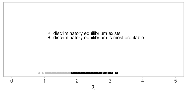
Figure 6: $\underline{\mu}=0.55$, $\overline{\mu}=.65$, $C=.03$, $\lambda$ ranges from $.1$ to $5$, and # of grids is 100. An impartial equilibrium always exists; it sustains the high effort profile if $\mu<1.67$ and the low effort profile if $\mu>1.67$.

In the case of information processing, it has been recognized by various authors that mutual information captures an ideal situation in which the decision maker can learn about how to optimally encode states before processing the already available information. The result of optimal encoding is a property called “compression invariance,” whereby all payoff-equivalent states are treated as identical. Reality, however, is full of situations in which payoff-equivalent states are treated differently based on their perceptual properties (Dean and Neligh, forthcoming). To address this “perceptual distance critique,” Caplin et al. (2022) invent the class of uniform posterior separable (UPS) costs that nests mutual information as a special case. While we cannot solve our model analytically for alternative UPS costs, we have conducted numerical analysis and obtained qualitatively similar results to those under the mutual information cost. Figure 6 of Appendix O.6 depicts the equilibrium regimes obtained under total information — a UPS cost that is proposed by Bloedel and Zhong (2020) and enjoys several desirable properties.

To model information production, several authors have advocated the use of prior invariant costs (see, e.g., Denti et al. 2022), whereas Bloedel and Zhong (2020) provide a foundation for UPS costs based on sequential learning-proofness. We take no stand on this debate, but only stress that prior dependence is key to our comparative statics results, as illustrated by the next example.

Example O.1.

The following entropy-based cost function is proposed by Denti et al. (2022) as an alternative to the mutual information cost:

$$K(\pi)\coloneqq I(\pi\mid q).$$

In words, $K(\pi)$ is the mutual information of the productivity state generated by a fixed, “reference,” prior $q$, and the promotion recommendations prescribed by signal structure $\pi$. By construction, $K$ is independent of the true prior distribution of the state, hence the name “prior invariance.” Meanwhile, it becomes the mutual information cost when the reference prior equals the true prior, and so provides us with an ideal candidate for delineating the role of prior dependence in shaping our results.

We characterize the optimal signal structure obtained under $K$. To this end, we fix a profile $\bm{\mu}\in\{\underline{\mu},\overline{\mu}\}^{2}$ of effort choices by the agents, and let $p$ denote the true prior distribution of the productivity state under $\bm{\mu}$. We also use $\overline{\pi}_{q}$ to denote the average probability that a signal structure $\pi$ recommends $m$ for promotion under the reference prior $q$. In the case where the principal’s optimal signal structure for $\bm{\mu}$ is nondegenerate, it is fully pinned down by (i) an augmented version of the multinomial logit formula:

$$\pi(\Delta\theta)=\frac{\overline{\pi}_{q}\exp\left(\frac{\Delta\theta}{\lambda}\frac{p(\Delta\theta)}{q(\Delta\theta)}\right)}{\overline{\pi}_{q}\exp\left(\frac{\Delta\theta}{\lambda}\frac{p(\Delta\theta)}{q(\Delta\theta)}\right)+1-\overline{\pi}_{q}}\text{ }\forall\Delta\theta\in\{-1,0,1\},$$

and (ii) Bayes’s plausibility under the reference prior:

$$\sum_{\Delta\theta\in\{-1,0,1\}}q(\Delta\theta)\pi(\Delta\theta)=\overline{\pi}_{q}.$$

Solving these conditions simultaneously yields:

$$\overline{\pi}_{q}=\frac{(\alpha-1)\beta q(1)-(\beta-1)q(-1)}{(\alpha-1)(\beta-1)[q(1)+q(-1)]},$$

where

$$\alpha\coloneqq\exp\left(\frac{p(1)}{\lambda q(1)}\right)\text{ and }\beta\coloneqq\exp\left(\frac{p(-1)}{\lambda q(-1)}\right).$$

Consider first the case where $m$ and $w$ exert the same level of effort, so that the true prior is symmetric between them, i.e., $p(1)=p(-1)$. In the main body of the paper, we demonstrated that the symmetry of the true prior leads to the use of an impartial signal structure under the mutual information cost. When the reference prior differs from the true prior, it turns out that the optimal signal structure remains impartial if and only if the reference prior is symmetric across agents, i.e., $q(1)=q(-1)$. Intuitively, if the principal believes that $m$ is more productive $w$, i.e., $q(1)>q(-1)$, when calculating the attention cost, she will distort the optimal signal structure away from being impartial, despite that $w$ works equally as hard as $m$ in reality.

As for the exact nature of the distortion, our findings are in general ambiguous, depending on the trade-off between two countervailing forces. On the one hand, if $m$ is believed to be more productive than $w$, i.e., $q(1)>q(-1)$, then the good state $\Delta\theta=1$ is weighted heavily on the left-hand side of Bayes’s plausibility. On the other hand, the conditional probability that the signal structure recommends $m$ for promotion is discounted heavily in the good state (by $q(1)$ in the exponential term), and, unlike in the case of mutual information, we cannot raise the true prior $p(1)$ in the good state to cancel this effect out. Depending on how these forces play out, the average probability of promoting $m$ can be greater than or smaller than $1/2$, regardless of whether the true prior or the reference prior is used to calculate the average. More nuanced features of the distortion, as captured by $X\coloneqq\pi(1)-\pi(0)$ and $Y\coloneqq\pi(0)-\pi(-1)$, lack clear-cut predictions.

For the case where $\mu_{m}\neq\mu_{w}$, all we can show is that the optimal signal structure is never impartial. Thus while biased priors alone may lead to the use of a discriminatory signal structure, the underlying mechanism can be rather nuanced, and the resulting comparative statics can sometimes be counterintuitive. $\diamondsuit$

Appendix O.4 Additional robustness checks

Continuous effort choices.

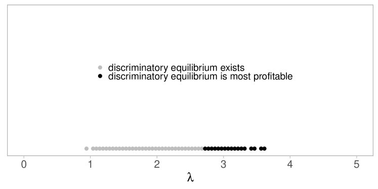
Figure 5: The cost of exerting $\mu\in[0,1]$ units of effort is $C(\mu)=.65\mu^{2}/2$, $\lambda$ ranges from 0.1 to 5, and # of grids is 100. An impartial equilibrium always exists.

While we have focused on the case of binary efforts for the sake of analytical tractability, we have also considered a variant of the model where effort choice can be any number between zero and one, and determines the agent’s probability of having a high productivity value. Figure 5 of Appendix O.6 depicts the numerical solutions obtained in a representative case; results therein resemble the equilibrium regimes predicted by the baseline model. Of course, there are many ways to weaken the assumption of binary choices. The takeaway from our numerical analysis is that that the results in the main body of the paper are not the mere artifact of binary choices, but instead survive (in essence) even without this assumption.

Mixed strategy equilibria.

So far we have restricted agents to playing pure strategies (while imposing no restriction on the principal’s strategy space). It turns out that generically, allowing mixed strategies on the part of agents makes it easier to sustain discrimination in equilibrium, in the following sense.

Proposition O.3.

For all $\lambda\neq\lambda^{*}$, any equilibrium in which at least one agent strictly mixes must be discriminatory.

The proof presented in Appendix O.5 also prescribes an algorithm for computing the mixed strategy equilibria of our model.

Appendix O.5 Proofs

Proof of Proposition O.2.

Parts (i) and (iii) of this proposition have already been shown in Appendix O.2. To show Part (ii), notice that when $\lambda\in(\lambda^{*},\overline{\lambda}]$, the principal can induce $(\overline{\mu},\underline{\mu})$ and $(\underline{\mu},\underline{\mu})$ as in the main body of the paper, and she prefers the first outcome to the second one. The only way to do better is to induce $(\overline{\mu},\overline{\mu})$ using a signal structure that makes one agent’s IC constraint binding and the other agent’s IC constraint slack.

Suppose w.l.o.g. that it is $m$ whose IC constraint is binding and $w$ whose IC constraint is slack. In that case, the principal’s problem can be formalized as follows:

$$\max_{\pi:\{-1,0,1\}\rightarrow[0,1]} \sum_{\Delta\theta\in\{-1,0,1\}}p(\Delta\theta)\pi(\Delta\theta)\Delta\theta+\overline{\mu}-\lambda I(\pi\mid p)$$

s.t. $$(1-\overline{\mu})[\pi(1)-\pi(0)]+\overline{\mu}[\pi(0)-\pi(-1)]\geq c,$$ (IC_m)

where the term $p(\Delta\theta)$ in the objective function denotes the probability that $\Delta\theta$ occurs under $(\overline{\mu},\overline{\mu})$, and $I(\pi\mid p)$ denotes the mutual information cost when the underlying states follow distribution $p$. Since the objective function is concave in $\pi$ and the constraint is linear in $\pi$, strong duality holds. Let $\nu_{m}$ denote the Lagrange multiplier associated with the constraint, and rewrite the principal’s problem as

$$\max_{\pi:\{-1,0,1\}\rightarrow[0,1]}\begin{Bmatrix}p(1)\pi(1)[1+\frac{\nu_{m}(1-\overline{\mu})}{p(1)}]+p(0)\pi(0)[0+\frac{\nu_{m}(2\overline{\mu}-1)}{p(0)}]\\ +p(-1)\pi(-1)[-1-\frac{\nu_{m}\overline{\mu}}{p(-1)}]\end{Bmatrix}-\lambda I(\pi\mid p).$$

By Matějka and McKay (2015), the solution to the last problem must satisfy

$$\pi(\Delta\theta)=\frac{\overline{\pi}\exp\left(v(\Delta\theta)/\lambda\right)}{\overline{\pi}\exp\left(v(\Delta\theta)/\lambda\right)+1-\overline{\pi}}\text{ }\forall\Delta\theta\in\{-1,0,1\}$$

if it is nondegenerate, where

$$v(1)\coloneqq 1+\frac{\nu_{m}(1-\overline{\mu})}{p(1)},v(0)\coloneqq\frac{\nu_{m}(2\overline{\mu}-1)}{p(0)},\text{ and }v(-1)\coloneqq-1-\frac{\nu_{m}\overline{\mu}}{p(-1)}.$$

In the case where the solution is impartial, we must have $\overline{\pi}=1/2$, as well as

$$\pi(0)=\frac{\overline{\pi}\exp\left(v(0)/\lambda\right)}{\overline{\pi}\exp\left(v(0)/\lambda\right)+1-\overline{\pi}}>1/2,$$

where the last inequality exploits the fact that $\overline{\mu}>1/2$ and $\nu_{m}>0$. Since impartiality requires that $\pi(0)=1/2$, we have reached a contradiction, hence the solution must be discriminatory, as desired. ∎

Proof of Proposition O.3.

When mixed strategies are allowed, let $\sigma_{i}\in[0,1]$ denote the probability that agent $i\in\{m,w\}$ exerts high effort, and assume w.l.o.g. that $\sigma_{m}\geq\sigma_{w}$. Then $\nu(\sigma_{i})\coloneqq\underline{\mu}+\sigma_{i}\Delta\mu$ is the probability that agent $i$ has a high productivity value, $\nu(\sigma_{m})[1-\nu(\sigma_{w})]$ is the probability that $m$ has a high productivity value and $w$ has a low productivity value, and $\nu(\sigma_{w})[1-\nu(\sigma_{m})]$ is the probability of the opposite situation. Write $A$ and $B$ for the last two quantities. Substituting them into Lemma 1 of the main text yields the principal’s optimal signal structure for any given profile $\bm{\sigma}\coloneqq(\sigma_{m},\sigma_{w})$ of the agents’ strategies, which satisfies

$$X=\frac{(\gamma A-B)(\gamma B-A)}{(\gamma^{2}-1)(A+B)A}\text{ and }Y=\frac{A}{B}X$$ (5)

if it is nondegenerate. Meanwhile, agents must be indifferent when they decide to strictly mix between high and low efforts. For $m$, this happens when

$$[1-\nu(\sigma_{w})]X+\nu(\sigma_{w})Y=c.$$ (6)

For $w$, this happens when

$$\nu(\sigma_{m})X+[1-\nu(\sigma_{m})]Y=c.$$ (7)

Solving (6) and (7) simultaneously yields either $X=Y=c$, or $\nu(\sigma_{m})+\nu(\sigma_{w})=1$, or both.

$\bullet$ In the first case, it follows from (5) that $A=B$ and $c=(\gamma-1)[2(\gamma+1)]^{-1}\coloneqq g(\gamma)$. The last equation holds if and only if $\gamma=g^{-1}(c)\coloneqq\gamma^{*}$, or, equivalently, $\lambda=\lambda^{*}$.

$\bullet$ In the second case, either $\nu(\sigma_{m})\neq\nu(\sigma_{w})$, and we are done. Alternatively, $\nu(\sigma_{m})=\nu(\sigma_{w})$, which, together with (5)-(7), implies that $A=B$ and $X=Y=c$, as in the first case.

Taken together, we conclude that for all $\lambda\neq\lambda^{*}$, any equilibrium in which both agents strictly mix must be discriminatory.

It remains to consider equilibria in which one and only one agent strictly mixes. There are two possibilities: (i) $\sigma_{m}\in(0,1)$ and $\sigma_{w}=0$, and (ii) $\sigma_{m}=1$ and $\sigma_{w}\in(0,1)$. $(\sigma_{m},\sigma_{w})$ is fully pinned down by (5) and (6) in the first case, and by (5) and (7) in the second case. Whenever a solution exists, it must be discriminatory. ∎

Appendix O.6 Figures

References

- (1)
- Aigner and Cain (1977) Aigner, Dennis J and Glen G Cain, “Statistical theories of discrimination in labor markets,” Industrial and Labor Relations Review, 1977, 30 (2), 175–187.
- Alchian and Demsetz (1972) Alchian, Armen A and Harold Demsetz, “Production, information costs, and economic organization,” American Economic Review, 1972, 62 (5), 777–795.
- Arrow (1971) Arrow, Kenneth J, “Some models of racial discrimination in the labor market,” Technical Report RM-6253-RC, RAND 1971.
- Arrow (1998) , “What has economics to say about racial discrimination?,” Journal of Economic Perspectives, 1998, 12 (2), 91–100.
- Baker et al. (1988) Baker, George P, Michael C Jensen, and Kevin J Murphy, “Compensation and incentives: Practice vs. theory,” Journal of Finance, 1988, 43 (3), 593–616.
- Bartoš et al. (2016) Bartoš, Vojtěch, Michal Bauer, Julie Chytilová, and Filip Matějka, “Attention discrimination: Theory and field experiments with monitoring information acquisition,” American Economic Review, 2016, 106 (6), 1437–1475.
- Becker (1957) Becker, Gary S, The Theory of Discrimination, University of Chicago Press, 1957.
- Bertrand (2018) Bertrand, Marianne, “Coase lecture–the glass ceiling,” Economica, 2018, 85 (338), 205–231.
- Bertrand and Mullainathan (2004) and Sendhil Mullainathan, “Are Emily and Greg more employable than Lakisha and Jamal? A field experiment on labor market discrimination,” American Economic Review, 2004, 94 (4), 991–1013.
- Bertrand et al. (2005) , Dolly Chugh, and Sendhil Mullainathan, “Implicit discrimination,” American Economic Review, 2005, 95 (2), 94–98.
- Blau and Kahn (2017) Blau, Francine D and Lawrence M Kahn, “The gender wage gap: Extent, trends, and explanations,” Journal of Economic Literature, 2017, 55 (3), 789–865.
- Bloedel and Zhong (2020) Bloedel, Alexander W and Weijie Zhong, “The cost of optimally-acquired information,” Unpublished Manuscript, 2020.
- Bohnet et al. (2016) Bohnet, Iris, Alexandra Van Geen, and Max Bazerman, “When performance trumps gender bias: Joint vs. separate evaluation,” Management Science, 2016, 62 (5), 1225–1234.
- Bohren et al. (2019) Bohren, Aislinn, Alex Imas, and Michael Rosenberg, “The dynamics of discrimination: Theory and evidence,” American Economic Review, 2019, 109 (10), 3395–3436.
- Borjas and Goldberg (1978) Borjas, George J and Matthew S Goldberg, “Biased screening and discrimination in the labor market,” American Economic Review, 1978, 68 (5), 918–922.
- Caplin et al. (2022) Caplin, Andrew, Mark Dean, and John Leahy, “Rationally inattentive behavior: Characterizing and generalizing Shannon entropy,” Journal of Political Economy, 2022, 130 (6), 1676–1715.
- Chambers and Echenique (2021) Chambers, Christopher P and Federico Echenique, “A characterisation of “Phelpsian” statistical discrimination,” The Economic Journal, 2021, 131 (637), 2018–2032.
- Chapman et al. (2013) Chapman, Elizabeth N, Anna Kaatz, and Molly Carnes, “Physicians and implicit bias: How doctors may unwittingly perpetuate health care disparities,” Journal of General Internal Medicine, 2013, 28 (11), 1504–1510.
- Chaudhuri and Sethi (2008) Chaudhuri, Shubham and Rajiv Sethi, “Statistical discrimination with peer effects: Can integration eliminate negative stereotypes?,” Review of Economic Studies, 2008, 75 (2), 579–596.
- Chowdhury et al. (2020) Chowdhury, Subhasish M, Patricia Esteve-González, and Anwesha Mukherjee, “Heterogeneity, leveling the playing field, and affirmative action in contests,” Southern Economic Journal, 2020.
- Chugh (2004) Chugh, Dolly, “Societal and managerial implications of implicit social cognition: Why milliseconds matter,” Social Justice Research, 2004, 17 (2), 203–222.
- Coate and Loury (1993) Coate, Stephen and Glenn C Loury, “Will affirmative-action policies eliminate negative stereotypes?,” American Economic Review, 1993, 83 (5), 1220–1240.
- Cornell and Welch (1996) Cornell, Bradford and Ivo Welch, “Culture, information, and screening discrimination,” Journal of Political Economy, 1996, 104 (3), 542–571.
- Correll and Simard (2016) Correll, Shelley and Caroline Simard, “Research: Vague feedback is holding women back,” Harvard Business Review, 2016, 29.
- Correll et al. (2020) Correll, Shelley J, Katherine R Weisshaar, Alison T Wynn, and JoAnne Delfino Wehner, “Inside the black box of organizational life: The gendered language of performance assessment,” American Sociological Review, 2020, 85 (6), 1022–1050.
- Cover and Thomas (2006) Cover, Thomas M and Joy A Thomas, Elements of Information Theory, John Wiley & Sons, 2006.
- de Haan et al. (2017) de Haan, Thomas, Theo Offerman, and Randolph Sloof, “Discrimination in the labour market: The curse of competition between workers,” The Economic Journal, 2017, 127 (603), 1433–1466.
- Dean and Neligh (forthcoming) Dean, Mark and Nate Leigh Neligh, “Experimental tests of rational inattention,” Journal of Political Economy, forthcoming.
- Deb and Renou (2022) Deb, Rahul and Ludovic Renou, “Which wage distributions are consistent with statistical discrimination?,” Working paper, 2022.
- Denti et al. (2022) Denti, Tommaso, Massimo Marinacci, and Aldo Rustichini, “Experimental cost of information,” American Economic Review, 2022, 112 (9), 3106–3123.
- Dianat et al. (2022) Dianat, Ahrash, Federico Echenique, and Leeat Yariv, “Statistical discrimination and affirmative action in the lab,” Games and Economic Behavior, 2022, 132, 41–58.
- Doleac (2021) Doleac, Jennifer L, “A review of Thomas Sowell’s discrimination and disparities,” Journal of Economic Literature, 2021, 59 (2), 574–89.
- Drugov and Ryvkin (2017) Drugov, Mikhail and Dmitry Ryvkin, “Biased contests for symmetric players,” Games and Economic Behavior, 2017, 103, 116–144.
- Eberhardt (2020) Eberhardt, Jennifer L, Biased: Uncovering the Hidden Prejudice that Shapes What We See, Think, and Do, Penguin, 2020.
- Escudé et al. (2022) Escudé, Matteo, Paula Onuchic, Ludvig Sinander, and Quitzé Valenzuela-Stookey, “Statistical discrimination and statistical informativeness,” arXiv preprint arXiv:2205.07128, 2022.
- Fang (2001) Fang, Hanming, “Social culture and economic performance,” American Economic Review, 2001, 91 (4), 924–937.
- Fang and Moro (2011) and Andrea Moro, “Theories of statistical discrimination and affirmative action: A survey,” Handbook of Social Economics, 2011, 1, 133–200.
- Fosgerau et al. (2023) Fosgerau, Mogens, Rajiv Sethi, and Jorgen W Weibull, “Equilibrium screening and categorical inequality,” American Economic Journal: Microeconomics, 2023, 15 (3), 201–242.
- Fryer (2007) Fryer, Roland, “Belief flipping in a dynamic model of statistical discrimination,” Journal of Public Economics, 2007, 91 (5-6), 1151–1166.
- Fryer and Jackson (2008) and Matthew O Jackson, “A categorical model of cognition and biased decision-making,” BE Journal of Theoretical Economics, 2008, 8 (1), 1–42.
- Fu and Wu (2020) Fu, Qiang and Zenan Wu, “On the optimal design of biased contests,” Theoretical Economics, 2020, 15 (4), 1435–1470.
- Glover et al. (2017) Glover, Dylan, Amanda Pallais, and William Pariente, “Discrimination as a self-fulfilling prophecy: Evidence from French grocery stores,” Quarterly Journal of Economics, 2017, 132 (3), 1219–1260.
- Greenwald and Lai (2020) Greenwald, Anthony G and Calvin K Lai, “Implicit social cognition,” Annual Review of Psychology, 2020, 71 (1), 419–445.
- Greenwald and Banaji (1995) and Mahzarin R Banaji, “Implicit social cognition: Attitudes, self-esteem, and stereotypes,” Psychological Review, 1995, 102 (1), 4–27.
- Greenwald et al. (1998) , Debbie E McGhee, and Jordan LK Schwartz, “Measuring individual differences in implicit cognition: The implicit association test,” Journal of Personality and Social Psychology, 1998, 74 (6), 1464–1480.
- Holzer and Neumark (2000) Holzer, Harry and David Neumark, “Assessing affirmative action,” Journal of Economic Literature, 2000, 38 (3), 483–568.
- Hu et al. (2023) Hu, Lin, Anqi Li, and Ilya Segal, “The politics of personalized news aggregation,” Journal of Political Economy Microeconomics, 2023, 1 (3), 463–505.
- Huang et al. (2022) Huang, Bo, Jiacui Li, Tse-Chun Lin, Mingzhu Tai, and Yiyuan Zhou, “Attention constraints and financial inclusion,” Working Paper, 2022.
- Knowles et al. (2001) Knowles, John, Nicola Persico, and Petra Todd, “Racial bias in motor vehicle searches: Theory and evidence,” Journal of Political Economy, 2001, 109 (1), 203–229.
- Lavy and Sand (2018) Lavy, Victor and Edith Sand, “On the origins of gender gaps in human capital: Short-and long-term consequences of teachers’ biases,” Journal of Public Economics, 2018, 167, 263–279.
- Li and Yang (2020) Li, Anqi and Ming Yang, “Optimal incentive contract with endogenous monitoring technology,” Theoretical Economics, 2020, 15 (3), 1135–1173.
- Lundberg and Startz (1983) Lundberg, Shelly J and Richard Startz, “Private discrimination and social intervention in competitive labor market,” American Economic Review, 1983, 73 (3), 340–347.
- Mackenzie et al. (2019) Mackenzie, Lori, JoAnne Wehner, and Shelley J Correll, “Why most performance evaluations are biased, and how to fix them,” Harvard Business Review, 2019.
- Maćkowiak et al. (2023) Maćkowiak, Bartosz, Filip Matějka, and Mirko Wiederholt, “Rational inattention: A review,” Journal of Economic Literature, 2023, 61 (1), 226–273.
- Macrae and Bodenhausen (2000) Macrae, C Neil and Galen V Bodenhausen, “Social cognition: Thinking categorically,” Annual Review of Psychology, 2000, 51, 93–120.
- Matějka and McKay (2015) Matějka, Filip and Alisdair McKay, “Rational inattention to discrete choices: A new foundation for the multinomial logit model,” American Economic Review, 2015, 105 (1), 272–98.
- Matveenko and Mikhalishchev (2021) Matveenko, Andrei and Sergei Mikhalishchev, “Attentional role of quota implementation,” Journal of Economic Theory, 2021, 198, 105356.
- Moss-Racusin et al. (2012) Moss-Racusin, Corinne A, John F Dovidio, Victoria L Brescoll, Mark J Graham, and Jo Handelsman, “Science faculty’s subtle gender biases favor male students,” Proceedings of the National Academy of Sciences, 2012, 109 (41), 16474–16479.
- Niederle and Vesterlund (2011) Niederle, Muriel and Lise Vesterlund, “Gender and competition,” Annual Review of Economics, 2011, 3 (1), 601–630.
- Onuchic (2022) Onuchic, Paula, “Recent contributions to theories of discrimination,” arXiv preprint arXiv:2205.05994, 2022.
- Phelps (1972) Phelps, Edmund S, “The statistical theory of racism and sexism,” American Economic Review, 1972, 62 (4), 659–661.
- Prendergast (1999) Prendergast, Canice, “The provision of incentives in firms,” Journal of Economic Literature, 1999, 37 (1), 7–63.
- Ravid (2020) Ravid, Doron, “Ultimatum bargaining with rational inattention,” American Economic Review, 2020, 110 (9), 2948–2963.
- Sims (2003) Sims, Christopher A, “Implications of rational inattention,” Journal of Monetary Economics, 2003, 50 (3), 665–690.
- Warikoo et al. (2016) Warikoo, Natasha, Stacey Sinclair, Jessica Fei, and Drew Jacoby-Senghor, “Examining racial bias in education: A new approach,” Educational Researcher, 2016, 45 (9), 508–514.
- Wynn and Correll (2018) Wynn, Alison T and Shelley J Correll, “Combating gender bias in modern workplaces,” in “Handbook of the Sociology of Gender,” Springer, 2018, pp. 509–521.
- Yang (2020) Yang, Ming, “Optimality of debt under flexible information acquisition,” Review of Economic Studies, 2020, 87 (1), 487–536.