Asymptotic Analysis of Deep Residual Networks111Alain Rossier’s research was supported through EPSRC Centre for Doctoral Training in Mathematics of Random Systems: Analysis, Modelling and Simulation (EP/S023925/1).
Abstract
We investigate the asymptotic properties of deep Residual networks (ResNets) as the number of layers increases. We first show the existence of scaling regimes for trained weights markedly different from those implicitly assumed in the neural ODE literature. We study the convergence of the hidden state dynamics in these scaling regimes, showing that one may obtain an ODE, a stochastic differential equation (SDE) or neither of these. In particular, our findings point to the existence of a diffusive regime in which the deep network limit is described by a class of stochastic differential equations (SDEs). Finally, we derive the corresponding scaling limits for the backpropagation dynamics.
1 Introduction
Residual networks, or ResNets, are multilayer neural network architectures in which a skip connection is introduced at every layer ([13]). This allows very deep networks to be trained by circumventing vanishing and exploding gradients, mentioned in [3]. The increased depth in ResNets has lead to commensurate performance gains in applications ranging from speech recognition [14, 33] to computer vision [13, 16].
A residual network with layers may be represented as
| (1.1) |
where is the hidden state at layer , the input, the output, a nonlinear activation function, its component-wise extension to , and , , and trainable network weights for .
ResNets have been the focus of several theoretical studies due to a perceived link with a class of differential equations. The idea, put forth in [12] and [4], is to view (1.1) as a discretization of a system of ordinary differential equations
| (1.2) |
where and are appropriate smooth functions and . This may be justified ([31]) by assuming that
| (1.3) |
as increases. Such models, named neural ordinary differential equations or neural ODEs [4, 7], have motivated the use of optimal control methods to train ResNets [8].
However, the precise link between deep ResNets and the neural ODE (1.2) is unclear: in practice, the weights and result from training, yet the validity of the scaling assumptions (1.3) for trained weights is far from obvious. As a matter of fact, there is empirical evidence showing that using a scaling factor can deteriorate the network accuracy [2]. Also, there is no guarantee that weights obtained through training have a non-zero limit which depends smoothly on the layer, as (1.3) would require. In fact, for ResNet architectures used in practice, empirical evidence points to the contrary [5]. These observations motivate an in-depth examination of the actual scaling behavior of weights with network depth in ResNets and of its impact on the asymptotic behavior of those networks.
Contributions. We systematically investigate the scaling behavior of trained networks weights and examine in detail the consequence of this scaling for the asymptotic properties of ResNets as the number of layers increases. We first show, through detailed numerical experiments, the existence of scaling regimes for trained weights markedly different from those implicitly assumed in the neural ODE literature. We study the convergence of the hidden state dynamics in these scaling regimes, showing that one may obtain an ODE, a stochastic differential equation (SDE) or neither of these. More precisely, we show strong convergence of the hidden state dynamics to a limiting ODE or SDE, by viewing the discrete hidden state dynamics as a “nonlinear Euler scheme” of the limiting equation. At a mathematical level, we extend the convergence analysis of Higham et al. [15] for discretization schemes of time-homogeneous (Markov) diffusions to a class of nonlinear approximations for Itô processes with bounded coefficients.
In particular, our findings point to the existence of a “diffusive regime” in which the deep network limit is described by a class of stochastic differential equations (SDEs). These novel findings on the relation between ResNets and neural ODEs complement previous work [31, 9, 11, 25, 29]. Finally, we derive the corresponding scaling limit for the backpropagation dynamics. The results we obtain are different from previous ones on asymptotics of ResNets [4, 12, 23], and correspond to a different scaling regime which is relevant for trained weights in practical settings.
In particular, in the diffusive regime we find a limit different from the “Neural SDE” literature [21]. Indeed, we observe that the Jacobian of the output with respect to the hidden states depends on hidden states across all levels, so may not be directly expressed as the solution of a forward or backward stochastic differential equation, as proposed in [21]. However, in Section 5 we obtain a representation for the asymptotics of the backpropagation dynamics in terms of an auxiliary forward SDE.
Outline. Section 2 describes the various scaling regimes for trained weights evidenced in [5] and the methodology for studying this scaling behaviour in the deep network limit. In Section 3, we report detailed numerical experiments on the scaling of trained network weights across a range of ResNet architectures and datasets, showing the existence of at least three different scaling regimes, none of which correspond to (1.3). In Section 4, we show that under these scaling regimes, the dynamics of the the hidden state may be described in terms of a class of ordinary or stochastic differential equations, different from the neural ODEs studied in [4, 12, 23]. In Section 5, we derive the large depth limit of the backpropagation dynamics under each scaling regime.
Notations. Let denote the Euclidean norm of a vector . For a matrix , denote its transpose, its diagonal vector, its trace and its Frobenius norm. Denote the integer part of a real number . Let denote the Gaussian distribution with mean and (co)variance , denote the tensor product, and ( times). Define the vectorisation operator by , and let be the indicator function of a set . is the space of continuous functions, for , is the space of -Hölder continuous functions, and is the Sobolev space of order .
2 Scaling regimes
We start by providing a framework for describing the scaling regimes for trained network weights, as identified in numerical experiments on deep ResNets [5].
2.1 Scaling regimes for trained network weights
As described in Section 1, the neural ODE limit assumes
| (2.1) |
for , where and are smooth functions [31]. Our numerical experiments, detailed in Section 3, show that the norm of the weights generally shrinks as increases (see for example Figures 2 and 4), so one cannot expect the above assumption to hold, unless weights are renormalized in some way. We consider here a more general assumption which includes (2.1) but allows for shrinking weights.
Scaling regime 1.
There exist and such that
| (2.2) |
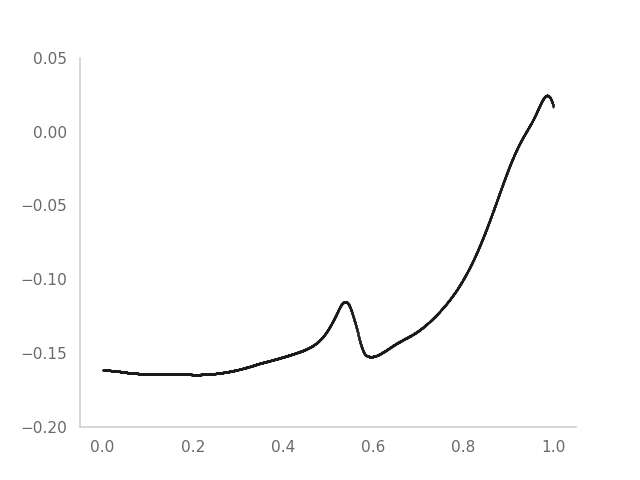
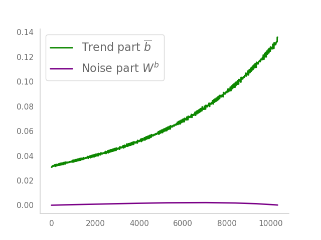
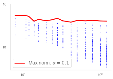
These renormalized weights do converge to a continuous function of the layer in some cases, as shown in Figure 1 (top) which displays a ResNet (1.1) with fully connected layers and activation function, without explicit regularization (see Section 3.2).
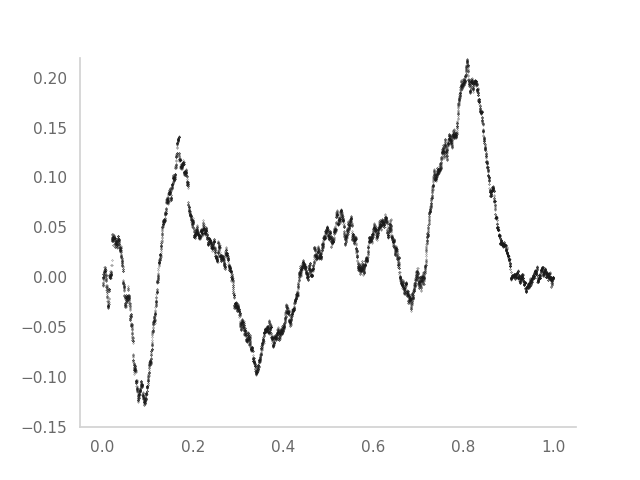
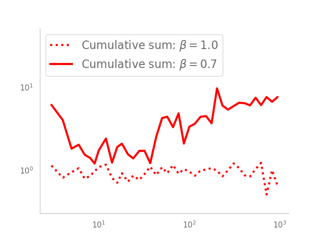
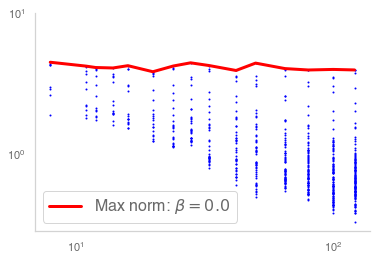
Yet, it is not the case that network weights always converge to a smooth function of the layer, even after rescaling. Indeed, network weights are usually initialized to random, independent and identically distributed (i.i.d.) values, whose scaling limit would then correspond to a white noise, which cannot be represented as a function of the layer. In this case, the cumulative sum of the weights behaves like a random walk, which does have a well-defined scaling limit . Figure 1 (bottom) shows that, for a ResNet with fully-connected layers, this cumulative sum of trained weights converges to an irregular, that is, non-smooth function of the layer.
This observation motivates the consideration of a different scaling regime where the weights are represented as the increments of a continuous function , i.e. the cumulative sum of the weights may converges to a limit but not the weight themselves. We also allow for a trend term as in Scaling regime 1.
Scaling regime 2.
There exist , , and non-zero such that and
| (2.3) |
The above decomposition is unique. Indeed, for ,
| (2.4) |
The integral of is thus uniquely determined by the weights , so can be obtained by discretization and by fitting the residual error in (2.4). In addition, Scaling Regimes 1 and 2 are mutually exclusive since Scaling regime 2 requires to be non-zero.
Remark 1.
In the case of independent Gaussian weights
where is the -th entry of and is the -th entry of , we can represent the weights as the increments of a matrix-valued Brownian motion
which is a special case of Scaling regime 2.
This remark shows that Scaling regime 2 corresponds to a ’diffusive’ regime.
2.2 Smoothness of weights with respect to the layer
A question related to the existence of a scaling limit is the degree of smoothness of the limits or , if they exist. To quantify the smoothness of the function mapping the layer number to the corresponding network weight, we define in Table 2.2 several quantities which may be viewed as discrete versions of various (semi-)norms used to measure the smoothness of functions.
| Quantity | Definition |
|---|---|
| Maximum norm | |
| Cumulative sum norm | |
| -scaled norm of increments | |
| Root sum of squares |
3 Scaling behavior of trained weights: numerical experiments
We now report on detailed numerical experiments to investigate the scaling properties and asymptotic behavior of trained weights for residual networks as the number of layers increases. We focus on two types of architectures: fully-connected and convolutional networks.
3.1 Methodology
We underline that Scaling Regimes 1 and 2 are mutually exclusive since Scaling regime 2 requires to be non-zero. In order to examine whether one of these scaling regimes, or neither, holds for the trained weights and , we proceed as follows.
Step 1: First, to obtain the scaling exponent , note that under Scaling regime 2,
Hence, we perform a logarithmic regression of the cumulative sum norm of with respect to , and the rate of increase of as is .
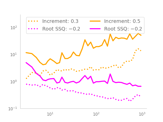
Step 2: After identifying the correct scale for the weights, we compute the -scaled norm of increments of to check whether they satisfy Scaling regime 1 and measure the smoothness of the trained weights. On one hand, if the -scaled norm of increments of does not vanish as , it means that the rescaled weights cannot be represented as a continuous function of the layer, as in Scaling regime 1. On the other hand, if the -scaled norm of increments of vanishes (say, as ) when increases, it supports Scaling regime 1 with a Hölder-continuous limit function .
Step 3: To discriminate between Scaling regimes 1 and 2, we decompose the cumulative sum of the trained weights into a trend component and a noise component , as shown in (2.4). The presence of non-negligible noise term favors Scaling regime 2.
Step 4: Finally, we estimate the regularity of the term under Scaling regime 2. If has diffusive behavior, as in the example of i.i.d. random weights, then its quadratic variation tensor defined by
has a finite limit as . Hence, using (2.3) and Cauchy-Schwarz, we obtain
| (3.1) |
where is the Hilbert-Schmidt norm. As is continuous on a compact domain, its norm is finite. Hence, if we have , the fact that the root sum of squares of is upper bounded as implies that the quadratic variation of is finite.
We follow all of the above steps for as well. Note that the scaling exponent may not be the same for and .
Remark 2.
Note that is homogeneous of degree , so we can write
Hence, when analyzing the scaling of trained weights in the case of a activation with fully-connected layers, we look at the quantities and , as they represent the total scaling of the residual connection.
3.2 Results for fully-connected layers
We first consider the case where the network layers are fully-connected. We consider the network architecture (1.1) for two different setups:
-
(i)
, trainable,
-
(ii)
, trainable.
We choose to present these two cases for the following reasons. First, both and are widely used in practice. Further, having scalar makes the derivation of the limiting behavior simpler. Also, since is an odd function, the sign of can be absorbed into the activation. Therefore, we can assume that is non-negative for . Regarding , having a shared would hinder the expressiveness of the network. Indeed, if for instance , we would get element-wise since is non-negative. This would imply that , which is not desirable. The same argument applies to the case . Thus, we let depend on the layer number for networks.
We consider two data sets. The first one is synthetic: fix and generate i.i.d samples coming from the dimensional uniform distribution in . Let and simulate the following dynamical system:
where . The targets are defined as . The motivation behind this low-dimensional dataset is to be able to train very deep residual networks and to be sure that there exists at least a (sparse) optimal solution.
The second dataset is a low-dimensional embedding of the MNIST handwritten digits dataset [20]. Let be an input image and its corresponding class. We transform into a lower dimensional embedding using an untrained convolutional projection, where . More precisely, we stack two convolutional layers initialized randomly, we apply them to the input and we flatten the downsized image into a dimensional vector. Doing so reduces the dimensionality of the problem while allowing very deep networks to reach at least training accuracy. The target is the one-hot encoding of the corresponding class.
The weights are updated by stochastic gradient descent (SGD) using batches of size on the mean-square loss and a constant learning rate , until the loss falls below , or when the maximum number of updates is reached. We repeat the experiments for depths varying from to . Details are given in Appendix A.
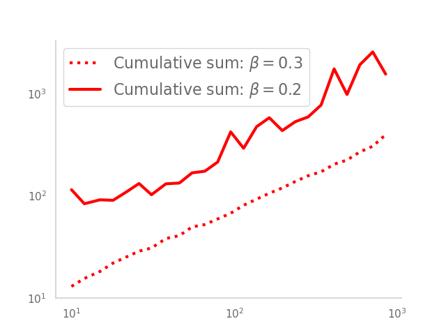
Results. For the case of a activation (i), we observe in Figure 2 that for both datasets, clearly decreases as increases, and decreases slightly when increases. We deduce that for the MNIST dataset and for the synthetic dataset.
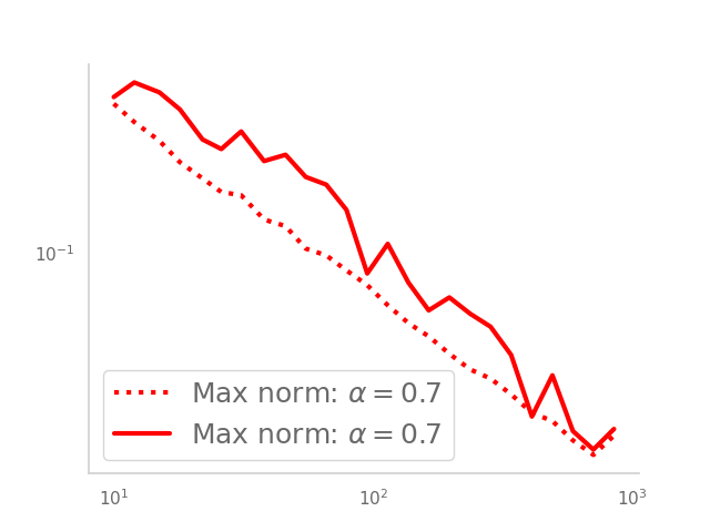
We use these results to identify the scaling behavior of . We observe in Figure 3 (left) that the -scaled norm of increments of decreases like , suggesting that Scaling regime 1 holds, with being Hölder continuous. This is confirmed in Figure 3 (right), as the trend part is visibly continuous and even of class . The noise part is negligible. This observation is even more striking given that the weights are trained without explicit regularization.
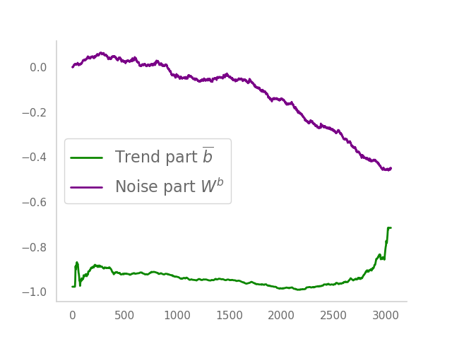
Regarding the case of a activation function (ii), we observe in Figure 4 (left) that the trend part of the residual connection scales like for the synthetic dataset and like for the MNIST dataset. We see in Figure 4 (right) that keeping the sign of is important, as the sign oscillates considerably throughout the network depth .
Figure 5 (left) shows that the -scaled norm of increments diverges as the depth increases. This suggests that there exists a noise part . Following (3.1), the fact that the root sum of squares of is upper bounded as and implies that has finite quadratic variation. These claims are also supported by Figure 5 (right): there is a non-zero trend part , and a non-negligible noise part .
Given the scaling behavior of the trained weights, we conclude that Scaling regime 1 seems to be a plausible description for the case (i), but Scaling regime 2 provides a better description for the case (ii).
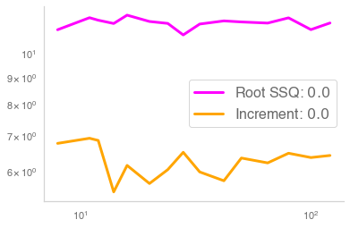
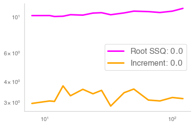
Scaling behavior of are shown for the case in Figure 6 and for the case in Figure 7. We observe that the cumulative sum norm, the scaled norm of the increments and the root sum of squares of scales in the same way as as the depth increases. In particular, the scaling exponent for is equal to the scaling exponent of , justifying the setup considered in Section 2.
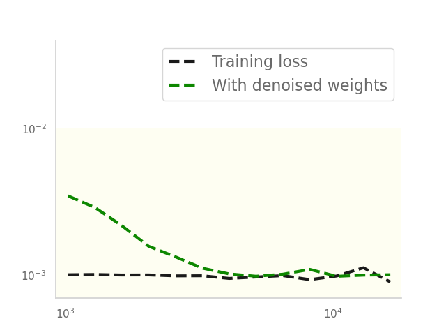
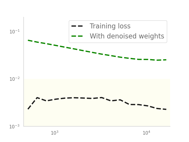
Importance of the stochastic term . It is legitimate to ask whether the noise term plays a significant role in the output accuracy of the network. To test this, we create a residual network with denoised weights , compute its training error and we compare it to the original training error. We observe in Figure 8 (left) that for , the noise part is negligible and does not influence the loss. However, for , the loss with denoised weights is one order of magnitude above the original training loss, meaning that the noise part plays a significant role in the accuracy of the trained network.
Sensitivity of and with respect to the hyperparameters. The values of and stem from the trained weights, which are themselves a function of the initialization and the training algorithm. We are using stochastic gradient descent, and the most significant hyperparameters of SGD are the learning rate and the batch size .
Hence, we report the value and found for the and trainable architecture on the synthetic data with different batch sizes and learning rates , with different realizations for the initialization. We report the average values of and for different seeds in Table 2 below.
We observe that the learning rate does affect and while keeping around , and the batch size does not affect or . A plausible explanation for these observations is that a higher batch size means a more precise descent direction at the cost of efficiency, but the shape of the solution is not supposed to change.
3.3 Results for convolutional networks
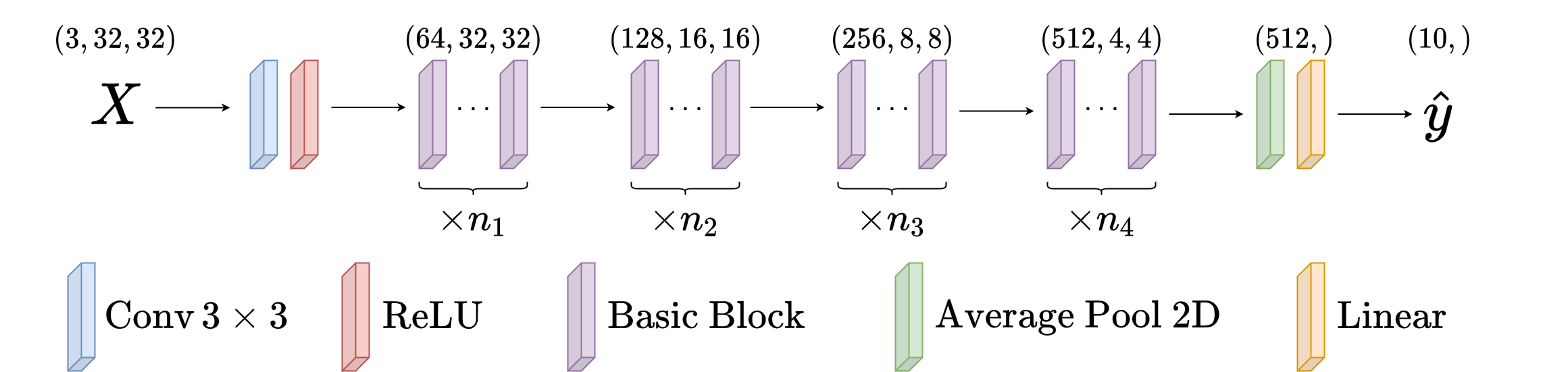
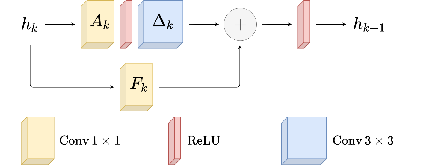
We now consider the original ResNet with convolutional layers introduced in [13]. This architecture is close to the state-of-the-art methods used for image recognition tasks. We do not include batch normalization [17] since it only slightly improves the performance of the network while making the analysis significantly more complicated. The architecture is displayed in Figures 9 and 10.
Our network still possesses the skip connections from (1.1): the dynamics of the hidden state reads
| (3.2) |
for , where . Here, , , and are kernels and denotes convolution. Note that plays the same role as from (1.1). To lighten the notation, we omit the superscripts (the input) and (the number of layers).
We train our residual networks at depths ranging from to on the CIFAR-10 [19] dataset with the unregularized relative entropy loss. Here, ’depth’ is the number of residual connections. We note that a network with is already very deep. As a comparison, a standard ResNet-152 [13] has depth in our framework.
Results. Table 3.3 shows the accuracy of our convolutional residual networks trained on an NVIDIA GeForce RTX 2080 GPU on the CIFAR-10 dataset. The results are in line with those of traditional ResNet architectures [13], even though our networks do not have batch normalization layers [17]. It is also noteworthy to add that our concept of depth is not that of traditional ResNets. We define the number of layers as the number of skip connections in the network, that is the number of kernels in (3.2).
| 8 | 11 | 12 | 14 | 16 | 20 | 24 | 28 | |
|---|---|---|---|---|---|---|---|---|
| Test error | 6.64 | 6.37 | 6.32 | 5.98 | 6.25 | 5.98 | 6.24 | 7.03 |
| 33 | 42 | 50 | 65 | 80 | 100 | 121 | ||
| Test error | 6.13 | 6.21 | 6.32 | 6.19 | 6.30 | 6.20 | 6.37 |
As in Section 3.2, we investigate how the weights scale with depth and whether Scaling regime 1 or Scaling regime 2 holds true for convolutional layers. To that end, we follow the steps of [30] to get the singular values, and therefore the spectral norms, of the linear operators defined by the convolutional kernels and . Figure 11 shows the maximum norm, and hence the scaling of and against the network depth . We observe that and with and .
We then use the values obtained for and to verify which Scaling regime holds. Figure 12 shows that both the -scaled norm of increments of and the -scaled norm of increments of seem to have lower bounds as the depth grows. This suggests that Scaling regime 1 does not hold for convolutional layers.
We also observe that the root sum of squares stays in the same order as the depth increases. Coupled with the fact that the maximum norms of and are close to constant order as the depth increases, this suggests that the scaling limit is sparse with a finite number of weights being of constant order in .
3.4 Summary: three scaling regimes
Our experiments show different scaling regimes for trained weights based on the network architecture.F or fully-connected layers with activation and a shared , we observe a behavior consistent with Scaling regime 1 for both the synthetic dataset and MNIST. For fully-connected layers with activation and , we observe that Scaling regime 2 holds for the synthetic dataset and MNIST. We deduce that the results for fully-connected layers are consistent with our findings in Figure 1.
In the case of convolutional architectures trained on CIFAR-10 and presented in Section 3.3, we observe that the maximum norm of the trained weights does not decrease with the network depth and the trained weights display a sparse structure, indicating a third scaling regime corresponding to sparse scaling limits for both and . These results are consistent with previous evidence on the existence of sparse CNN representations for image recognition [24]. We stress that the setup for our CIFAR-10 experiments has been chosen to approach state-of-the-art performance with our generic architecture, as shown in Figures 9 and 10.
4 Deep network limit
In this section, we study the scaling limit of the hiddent state dynamics (1.1) under scaling regimes 1 and 2.
4.1 Scaling regime 1: ODE limit
First, we show that the scaling regime 1 together with a smooth and Lipschitz-continuous activation function lead to two ODE limits under different parameter regimes, including the neural ODE described in [4, 31, 12] as a special case.
We focus our analysis on smooth activation functions.
Assumption 1 (Activation function).
The activation function satisfies , , , and has a bounded third derivative .
Most smooth activation functions, including , satisfy this condition. The boundedness of the third derivative may be relaxed to an exponential growth condition [26].
As observed in the numerical experiments, non-smooth activation functions such as lead to a different scaling regime to that of smooth functions.
We now describe ODE limits under Scaling regime 1. Let be a continuous-time extension of the hidden states :
| (4.2) |
4.2 Scaling regime 2
Let be a probability space with a -complete filtration . Let , resp. , be -dimensional, resp. -dimensional, -standard uncorrelated Brownian motions. We consider a setup which is consistent with Section 3 where the noise part comes from the increment of some stochastic process and for some :
| (4.5) | ||||
with
where and are Itô processes [28] adapted to and can be written in the form:
| (4.6) | ||||
with , , and for . We use the following notation for the quadratic variation of and :
| (4.7) |
where and are bounded processes with values respectively in and . From (4.6) and (4.7), we have the quadratic variation process as follows:
| (4.8) |
Here , , and are progressively measurable processes that satisfy the following conditions.
Assumption 2 (Regularity of the Ito processes and continuous functions ).
We assume:
-
(i)
There exists a constant such that almost surely
(4.9) -
(ii)
There exist and such that almost surely
(4.10) and
(4.11)
Note that (4.9) implies that are almost surely uniformly bounded and (4.10) implies that are almost surely Hölder continuous with exponent .
Lemma 1 (Uniform integrability).
Proof.
Write , where each component is defined, for , as
| (4.13) |
Let be a continuous-time extension of the hidden states :
| (4.14) |
Assumption 3 (Uniform integrability).
There exist and a constant such that for all ,
| (4.15) |
Assumption 3 is standard in the convergence of approximation schemes for SDEs [15]. In practice, condition (4.15) is guaranteed throughout the training as both the inputs and the outputs of the network are bounded.
Let us now describe the intuition behind the deep network limit when . Denote and define for :
Using Itô’s formula [18] to for , we obtain the following approximation
| (4.16) |
where
We observe from that (4.16) admits a diffusive limit only when . In this case, we see that and do not explode only when , corresponding to a stochastic differential equation (SDE) limit that is diffusive. Another case where we obtain a non-trivial limit is when and , which leads to an ODE limit.
We now provide a precise mathematical description of the different scaling limits of for various values of and , using the concept of uniform convergence in , also known as strong convergence. For a general exponent , we have the following definition.
Definition 1 (Uniform convergence in ).
Let and be the class of random functions such that
We say that a sequence converges uniformly in to if
| (4.17) |
We now show that Scaling regime 2 together with a smooth activation function lead to an ODE limit (which is different from the neural ODE) or a stochastic differential equation (SDE) depending on the values of and .
Theorem 2 (ODE limit under Scaling regime 2).
In particular, this implies the convergence of the hidden state process for any typical initialization (i.e almost surely with respect to the initialization). Note that in Theorem 2, the limit (4.18) defines a linear input-output map behaving like a linear network [1]. This is different from the neural ODE (1.2), where the activation function appears in the limit.
Theorem 3 (SDE limit under Scaling regime 2).
The proofs of Theorem 3 is given in Section 4.4. And the proof of Theorem 2 follows similar ideas. In particular, and vanish in the limit when in (4.16).
Interestingly, when the activation function is smooth, all limits in both Theorems 2 and 3 depend on the activation only through (assumed to be for simplicity) and . In contrast to the behavior of the neural ODE limit (1.2), the characteristics of away from are not relevant to the limit. In addition, our proofs rely on the smoothness of at . If the activation function is not differentiable at , then a different limit should be expected.
The case , , , and in Theorem 3 is considered in [26], under the additional assumption that and are Brownian motions with constant drift. We consider a more general setup, where we introduce nonzero terms and and we allow and to be arbitrary Itô processes. Moreover, [26] prove weak convergence, which corresponds to convergence of quantities averaged across many trained networks with random independent initializations, whereas in practice, the training is done only once. Thus, the strong convergence, shown in Theorems 1 and 3, is a more relevant notion for studying the asymptotic behavior of deep neural networks.
Although the ResNet dynamics (4.5) is not expressed as an Euler scheme of a (ordinary or stochastic) differential equation, we nevertheless show strong convergence to a limitng ODE (in the case of Theorem 2) or SDE (in the case of Theorem 3), using techniques inspired by [15]. The challenge is to bound the difference between the ResNet dynamics and the Euler scheme of the limiting SDE. It is worth mentioning that the results in [15] hold for a class of time-homogeneous (Markov) diffusion processes whereas our result holds for Itô processes with bounded coefficients. This distinction is important for training neural networks since the “diffusion” assumption involves the distribution of the hidden state dynamics which can never be tested in practice. We can only verify the smoothness of the hidden state dynamics as detailed in Section 3. In addition, we also relax one technical condition assumed in [15], which is difficult to verify in practice. See Remark 3.
Note that we assume that the Ito processes and are driven by uncorrelated Brownian motions and . This assumption might look strong, but we pose it for ease of exposition: assuming a generic correlation structure between and would only a cross-term in the definition of .
4.3 Link with numerical experiments
Let us now discuss how the analysis above sheds light on the numerical results in Section 3.2 and Section 3.3.
Figure 2 shows that and for the synthetic dataset with fully-connected layers and activation function. This corresponds to the assumptions of Theorem 1 with the ODE limit (4.18). This is also consistent with the estimated decomposition in Figure 3 (right) where the noise part is negligible.
Regarding activation with fully-connected layers, we observe that from Figure 4 (left). Since ReLU is homogeneous of degree 1 (see Remark 2), can be moved inside , so without loss of generality we can assume and . If we replace the function by a smooth version , then the limit is described by the stochastic differential equation (4.19). The case would then correspond to a limit of this equation as . The existence of such a limit is, however, nontrivial and left for future work.
From the experiments with convolutional architectures, we observe that the maximum norm (Figure 11), the scaled norm of the increments, and the root sum of squares (Figure 12) are upper bounded as the number of layers increases. This indicates that the weights fall into a sparse regime when is large. In this case, there is no continuous ODE or SDE limit and Scaling regimes 1 and 2 both fail.
4.4 Detailed proofs
4.4.1 Proof of Theorem 1
It suffices to prove the second case with limit (4.4). First we show that there exists such that
| (4.20) |
Indeed, denote as the Lipschitz constant of . Then
where , , and . Hence
By induction:
Hence (4.20) holds.
Denote and . From (4.16) we have
Denote as well and the -th element of and , respectively. Applying a third-order Taylor expansion of around with the help of Assumption 1, for , we get
| (4.21) |
with . The last equation holds since . Denote for as the uniform partition of the interval . For , define and
Then we have for all . Recall the solution to the ODE (4.4). Denote for and define the errors
We first bound . Note that by definition:
| (4.22) |
where . Therefore we have
Next, we bound . For ,
| (4.23) |
Denote , hence from (4.21) and (4.23),
Denote . Then,
Hence, we deduce
The last equation holds by (4.22). Then, we have for ,
| (4.24) |
with and a constant independent of and . Finally, when we have from (4.24):
| (4.25) |
and for ,
| (4.26) | |||||
(4.26) holds since and when . Therefore, we conclude
4.4.2 Proof of Theorem 2
We provide a complete proof of Theorem 2 for the case and . Other cases follow similarly. When and , we define the targeted SDE limit for the discrete scheme (4.5) as follows:
| (4.27) |
in which
| (4.28) | ||||
with and . Here the quadratic variation process is the Itô correction term for the drift. On the one hand this correction term introduces non-linearity into the drift and makes the proof challenging. On the other hand, this term is the key for the convergence analysis. See (4.55) and (4.56).
Euler-Maruyama scheme of the limiting SDE. Denote as the sub-interval length and , as the uniform partition of the interval . Further denote and as the increment of the stochastic processes. Define the Euler-Maruyama discretization scheme of the SDE (4.27) as:
| (4.29) |
and the one-step forward increment follows:
| (4.30) |
Therefore (4.29) can be rewritten as .
Continuous-time extension. Recall that we extend the scheme to a continuous-time process on by a piecewise constant and right-continuous interpolation of :
| (4.31) |
We call the continuous-time extension (CTE) of .
Continuous-time approximation. Denote
| (4.32) | |||||
and from (4.16) we thus have
Denote and the -th element of and , respectively. Applying a third-order Taylor expansion of around with the help of Assumption 1, for , we get
with . The increment of the ResNet has two parts: the increment of the Euler-Maruyama scheme and the residual
| (4.33) |
It is clear from here that the Euler-Maruyama scheme of the limiting SDE is different from the ResNet dynamics. Hence classical results on the convergence of discrete SDE schemes cannot be applied directly.
In our analysis it will be more natural to work with the following continuous-time approximation (CTA), defined as
| (4.34) |
where and is the integer for which for a given .
Here approximates the CTE (4.31) with a continuous version, with interpolations both in time and in space, of the part while the residual term remains the same. By design we have , that is, and coincide with the discrete solution at grid points , . This relationship is instrumental in order to control the error.
We will first study the difference between and , and then the difference between and , in the supremum norm. The sum of the two will give a bound for the error of the discrete approximation.
4.4.3 Preliminary result
Lemma 2 (Local Lipschitz condition and uniform integrability).
Remark 3.
Note that [15] assumes the uniform integrability condition for which is difficult to verify in practice. Here we relax this condition by only assuming the uniform integrability condition for the ResNet dynamics , see Assumption 3. We can then prove (4.36) under Assumption 3 and some properties of the Itô processes.
Proof of Lemma 2.
First, there exists such that
| (4.37) |
since is quadratic in and . Then,
Note that since and almost surely according to (4.9), respectively. Therefore (4.35) holds by taking .
Thanks to the assumption in Theorem 3, there exists a constant such that then we only need to show that (4.36) holds for for some . To see this, let be the integer for which for a given . Then
Hence, by the Minkowski inequality,
| (4.38) |
for some , as is quadratic in . The value of will be determined later. From (4.38), we get
| (4.39) | |||||
for some constants independent of , and . The first inequality holds by the Hölder and (4.39) holds by the Minkowski inequality. Take . Then, (4.39) is bounded thanks to Assumption 3 for , and we have and by (4.12). Hence, by the Minkowski inequality, we have
∎
4.4.4 Proof of Theorem 3
We are now ready to show the proof of Theorem 3.
Proof.
Let us define two stopping times to utilize the local Lipschitz property of :
| (4.40) |
and define the approximation errors
| (4.41) |
The proof contains two steps. The first step is to show and the second step is to show .
Following the idea in [15], we first show that for any (to be determined later):
| (4.42) |
where and are defined in (4.36). To see this, recall that by Young’s inequality, for , we have
| (4.43) |
First decompose the left-hand side of (4.42) to obtain, for all ,
| (4.44) | |||||
where we apply (4.43) with to the second term. Now
| (4.45) |
A similar result can be derived for , so that we have
| (4.46) |
Using the inequalities in (4.45)–(4.46), along with
| (4.47) |
To obtain a uniform bound on , we bound the first term on the right-hand side of (4.42). Using the definition of the targeted SDE limit in (4.27):
and the continuous-time approximation (4.34), we get
We first bound the above using Cauchy-Schwarz inequality:
Now, from the local Lipschitz condition (4.35) and Doob’s martingale inequality [28], we have for any ,
| (4.48) |
where . First, we give an upper bound for \fontsize{8.5pt}{0}\fontfamily{and}\selectfont2⃝. By the Cauchy–Schwarz inequality,
Hence, for , the following holds almost surely by (4.10):
| (4.49) |
Under Assumption 3, there exists a constant such that
Hence by Tonelli’s theorem,
| (4.50) |
Upper bound on \fontsize{8.5pt}{0}\fontfamily{and}\selectfont3⃝. Define the following discrete filtration
| (4.51) |
Note that is -measurable but not -measurable. Define for and for :
We can then decompose
Hence, we deduce the following bound on \fontsize{8.5pt}{0}\fontfamily{and}\selectfont3⃝ by Cauchy-Schwarz.
| (4.52) |
We provide an upper bound for each of the four terms in (4.52). For the first term, denote and so that is a –martingale. Hence, by Doob’s martingale inequality, we have
| (4.53) |
Fix . For , we compute the following conditional expectation.
| (4.54) |
The cross-term disappear as by definition of . Furthermore, conditionally on and on , observe that is the centered square of a normal random variable whose variance is uniformly in by (4.9), so there exist depending only on such that
Hence, plugging back into (4.53), we obtain
| (4.55) |
For the second term involving , we explicitly compute the conditional expectation using the definition of in (4.28) and the definition of in (4.13).
By Cauchy-Schwarz, Tonelli and (4.10) in Assumption 2 we obtain:
| (4.56) |
where depends only on . Moving to the third term of (4.52) involving , observe that
for some independent of since and almost surely. Then there exists depending only on such that
| (4.57) |
Finally, we bound the fourth term of (4.52) using Cauchy-Schwarz, Assumption 1 and property (4.9) of the Itô processes:
| (4.58) |
for some constant depending only on . Combining the results in (4.55), (4.56), (4.57) and (4.58), there exists constants depending only on such that
| (4.59) |
Upper bound on \fontsize{8.5pt}{0}\fontfamily{and}\selectfont1⃝. Given , we have
| (4.60) | |||||
by continuity of . Hence
| (4.61) |
Now, from the local Lipschitz condition (4.35), for we have almost surely
Combining the two previous inequalities we obtain
Hence, using (4.36) and the Lyapunov inequality [27], we get
| (4.62) | |||||
Combining the results in (4.50), (4.59) and (4.62), we have in (4.48) that
Applying the Grönwall inequality,
| (4.63) |
where is a universal constant independent of , and and is a constant only depending on . Combining (4.63) with (4.42), we have
| (4.64) |
Given any , we can choose so that , then choose so that , and finally choose sufficiently large so that
Therefore in (4.64), we have,
| (4.65) |
It remains to provide a uniform bound for . Recall the relationship between and defined in (4.60): by (4.9) we have almost surely that
Therefore,
| (4.66) |
First, by Assumption 3,
| (4.67) |
Second, by the Power Mean inequality and Doob’s martingale inequality,
Hence
| (4.68) |
By Hölder inequality,
| (4.69) |
Combining (4.67), (4.68), and (4.69) in (4.66), we obtain
for some constant . By choosing , we have
| (4.70) |
Finally, combining (4.65) and (4.70) leads to the desired result.
∎
5 Asymptotic analysis of the backpropagation dynamics
The most widely used method to train neural networks is the pairing of
-
•
the backpropagation algorithm to find the exact gradient (or a stochastic approximation) of the loss function with respect to the network weights, and
-
•
a variant of the gradient descent algorithm to iteratively update the network weights.
We are interested to study the behaviour of the former in residual networks, under our Scaling regimes 1 and 2. To do so, we will first formalize the objective function and the discrete backward equation linking the gradient of the loss function across layers.
5.1 Backpropagation in supervised learning
Suppose we want to learn the mapping through a dataset of input-target pairs , where for some compact and . The goal of any parametric supervised learning is to find, given a class of mappings , the parameter that minimizes the average training error:
| (5.1) |
Here, is a loss function, for example the squared error . In the following, we omit the dependence in . Fix and define
For an input , recall the following forward dynamics for the residual network
| (5.2) | ||||
We define . Our goal is to compute . Observe from the definition (5.1) and the chain rule that
The terms and are straightforward to obtain, so the crux of the challenge lies in computing . Using (5.2), for , we get
| (5.3) |
where for . The terminal condition is given by . We now obtain the asymptotic dynamics of under three different cases. In particular, we derive (backward) ODE limits for any set of weights under Scaling regime 1 and the asymptotic limit derived from an SDE under Scaling regime 2. For clarity, we omit the dependence in the input for .
5.2 Backward equation for the Jacobian under Scaling regime 1
Let be a continuous-time extension of the Jacobians defined in (5.3):
| (5.4) |
Theorem 4 (Backpropagation limits under Scaling regime 1).
Under the same assumptions as Theorem 1,
-
•
Neural ODE regime: If , , and is the solution to the neural ODE (4.3), then the backpropagation dynamics converge uniformly to the solution to the linear (backward) ODE
(5.5) in the sense that .
-
•
Linear ODE regime: If , , and is the solution to the linear ODE (4.4), then the backpropagation dynamics converge uniformly to the solution to the linear (backward) ODE
(5.6) in the sense that .
The ideas of the proof follow closely those of Theorem 1 and the complete proof is given in Section 5.4.1. We readily see that under Scaling regime 1, the backward dynamics of the gradient become linear. When , which is the case observed in practice, the dependence on the activation function disappears in the large depth limit, exactly as for the forward dynamics.
5.3 Backward equation for the Jacobian under Scaling regime 2
Recall the set-up of Theorem 3. Let be a probability space with a -complete filtration . Let , resp. , be -dimensional, resp. -dimensional, independent -Brownian motions. Recall that for Scaling regime 2,
| (5.7) |
where and are Itô processes [28] adapted to and can be written in the form:
| (5.8) | ||||
with , , and for . We use the notation in (4.7) and (4.8) for the quadratic variation of and .
Define
| (5.9) |
We will use the following assumption for the results in this section:
Assumption 4.
The boundedness of the fourth moment of the Jacobians in is similar to Assumption (3) and is standard in the convergence of approximation schemes for SDE. The second part of Assumption 4 is a technical condition: we need the fourth moment of the to be bounded. Theorem 5 proves that the process satisfy a linear SDE with drift linear in , so we need finiteness of the norm of the exponential of the drift, see Lemma 3 for more details. In practice, and stay bounded during training, so Assumption (4) is satisfied.
Theorem 5 (Backpropagation dynamics under Scaling regime 2).
The steps to prove Theorem 5 are similar to those of Theorem 3 but the details are technically more involved. Indeed, terms that depend on are not a priori adapted to the filtration generated by the Ito processes and . To overcome this challenge, we denote
| (5.12) |
and we can rewrite . This leads to a new perspective to understand through two components and . The first term is adapted to the filtration generated by the Ito processes, and is the Jacobian of the output with respect to the input, and does not depend on the layer. The complete proof is provided in Section 5.4.2.
5.3.1 Connection with Neural SDE
In a recent work, [21] show that, when the hidden state satisfies a continuous-time ’neural SDE’ dynamics, the Jacobian of the output with respect to the hidden states satisfies a backward SDE:
| (5.13) |
where is the time-reversed Brownian motion defined by , and is the solution of the backward flow of diffeomorphisms generated by the forward SDE (4.19).
It is clear that the limit in (5.11) differs from the adjoint process (5.13). Our limit does not satisfy any forward nor backward SDE, as its solution is a function of which depends on weights across all layers i.e. the entire path of . Indeed, Theorem 3.1 in [32] states that solves the following SDE.
Therefore, one can write
| (5.14) |
One can readily see that depends on for all . Note that the quadratic variation drift correction term stems from using Ito integrals instead of Stratonovitch integrals.
In contrast to (5.13),
(5.14) is the exact large-depth limit of gradients computed by backpropagation in finite depth residual networks, as stated in Theorem 5.
5.4 Proofs
5.4.1 Proof of Theorem 4
The ideas of the proof follow closely those of Theorem 1, and we will provide here the main arguments to the Neural ODE case. The other case is very similar.
Denote , as the uniform partition of the interval . For , define
where and are specified in Theorem 1. Hence, we can directly deduce that
By continuity of , and , the first supremum is finite and by a similar argument as in the proof of Theorem 1, the second supremum is also finite. Thus, there exists a constant such that . Now, we also have, for ,
Hence, for , we can estimate
where and . Now, recall that is uniformly bounded in , and we have and , so there exists a constant such that . Thus,
By Gronwall’s lemma and the fact that , we deduce that and conclude
5.4.2 Proof of Theorem 5
The ideas of the proof follow closely those of Theorem 3, and we will provide here the main arguments for the case and . Other cases follow similarly. For the ease of notation exposition, we consider and we use to denote some generic constant (independent from and other parameters, such as , , and , to be defined later) that may vary from step to step.
The proof consists of 11 steps that can be summarized as follows. Step 1 decomposes the discrete gradient into two terms: the Jacobian of the output with respect to the input, and the Jacobian of the hidden state with respect to the input, which we denote by . We then write a forward equation for . Step 2 defines a continuous-time approximation and a continuous-time interpolation . Step 3 establishes a uniform bound between and . Step 4 defines high-probability events under which the hidden states and the continuous-time limit are uniformly bounded. Step 5 decomposes the difference between and with a drift term and an error term , which can be further decomposed into a variance term and a Taylor remainder term . Step 6 proves that uniformly vanishes as . Step 7 decomposes into three terms. Step 8 and 9 prove that these terms uniformly vanishes as . Step 10 wraps everything together to show a uniform bound between and . Step 11 uses it to prove a uniform bound between the discrete gradients and their limit .
Step 0: Well-posedness of the statement. The matrix-valued linear stochastic differential equation (5.10) has a continuous and adapted solution, and this solution is unique in the sense that almost all sample processes of any two solutions coincide, see for example [10]. Furthermore, a.s., is invertible for all , see Corollary 2.1 in [6]. Also, Theorem 3.1 in [32] states that solves the following SDE.
Recall from Assumption 2 that the quadratic variation of is uniformly continuous with resepect to the Lesbegue measure. Therefore, by Lemma 3 and Assumption 4, we conclude that the fourth moments of the supremum of and are finite.
| (5.15) |
Step 1: Rewrite the discrete backpropagation equation. First, observe that multiplying (5.3) together gives, for ,
| (5.16) |
Define and for :
| (5.17) |
Note that by the chain rule, we directly have and . In the following, we omit the explicit dependence on the initial data when the context is clear. Recall now the definition from (4.32). By Taylor’s theorem on , as is continuous, for each , there exists such that
Hence, using , , and (5.7), we get
| (5.18) |
where we define the error term .
Step 2: Continuous-time approximation. Recall the (forward) SDE defined in the statement of the theorem
Recall the definition of in (4.31), and define similarly the continuous-time extension (CTE) of :
| (5.19) |
Let the index for which . Define the continuous-time approximation (CTA) of as
| (5.20) |
Step 3: Uniform bound between and . Using (5.18) and (5.20), we have, for ,
Hence,
By Assumptions 3 and 4, and equation (4.68):
| (5.21) |
Step 4: Initial computations for a uniform bound between and . Fix , and let (to be determined later) that only depends on and . Define for
| (5.22) |
Using Assumption 3 and (5.15), we obtain similarly to (4.45) that
| (5.23) |
Now, by Cauchy-Schwarz inequality, we have
We use it to decompose the distance between and :
Now, we have the following estimate
Therefore, by Assumption 4 and (5.15),
| (5.24) |
Step 5: Initial computations for a uniform bound between and . First we estimate, for ,
| (5.25) |
The goal is to find an upper bound of the first two terms, consisting of the sum of the distance between and and terms vanishing uniformly in . We also want to show that the error term uniformly vanishes in . To handle the term involving the drift , we first observe that for , , and , we have
We used the fact that is linear in and is Hölder continuous. We directly deduce that
| (5.26) | |||
| (5.27) |
The last inequality holds by Theorem 3. Hence, we obtain from (5.25)
| (5.28) |
We applied Doob’s martingale inequality [28] on the second term of (5.25), as , , and are adapted to the filtration generated by . We now estimate the error term in (5.28). Recall that it decomposes into a variance term and a Taylor remainder term .
Step 6: Prove that the remainder uniformly vanishes. We proceed to show that
| (5.29) |
which is straightforward since:
The last inequality holds for the same reasons as (4.57).
Step 7: Prove that the remainder uniformly vanishes. First note that we can write , where
| (5.30) |
We assumed that the Ito processes and are driven by uncorrelated Brownian motions, hence uniformly vanishes in at rate . Thus, we get
| (5.31) |
Using the discrete (forward) filtration defined in (4.51), we now expand (5.30) using the definition of Scaling regime 2.
Step 8: Prove that the term \fontsize{8.5pt}{0}\fontfamily{and}\selectfont1⃝ uniformly vanishes. Define
and . Observe that is a martingale, where the filtration is defined in (4.51). Hence, by Doob’s martingale inequality, we have
| (5.33) |
Fix and compute the following conditional expectation.
| (5.34) |
The cross-term disappear as . Furthermore, conditionally on , observe that is the variance of a product of two normal random variable with variance, uniformly in by (4.9), so
Hence, plugging it back into (5.33), we obtain
| (5.35) |
Step 9: Prove that the terms uniformly vanishes. The term \fontsize{8.5pt}{0}\fontfamily{and}\selectfont2⃝ can be estimated directly using Cauchy-Schwarz, Tonelli, and (4.10):
| (5.36) |
The estimation for term \fontsize{8.5pt}{0}\fontfamily{and}\selectfont3⃝ is straightforward and similar to (4.57):
| (5.37) |
Step 10: Uniform bound between and . From equations (5.29) (5.31), (5.35), (5.36), and (5.37), we deduce that
| (5.38) |
We then plug (5.38) into (5.28), together with Tonelli’s theorem, to get
We use (5.21) for the last inequality. Hence, by Gronwall lemma, we deduce:
| (5.39) |
Step 11: Difference between and . We first estimate the distance between the discrete gradients and the continuous-time limit . For each , we have the identity
Hence, by Assumption 4, (5.15), (5.21), and (5.39):
We plug it in (5.24) to obtain
| (5.40) |
To conclude, given any , we can choose such that , and then choose so that , and finally sufficiently large so that
Therefore, we have in (5.40)
References
- [1] S. Arora, N. Cohen, N. Golowich, and W. Hu, A Convergence Analysis of Gradient Descent for Deep Linear Neural Networks, in 7th International Conference on Learning Representations (ICLR), 2019.
- [2] T. Bachlechner, B. P. Majumder, H. Mao, G. Cottrell, and J. McAuley, ReZero is all you need: fast convergence at large depth, in Proceedings of Machine Learning Research, vol. 161, PMLR, 2021, pp. 1352–1361.
- [3] Y. Bengio, P. Simard, and P. Frasconi, Learning long-term dependencies with gradient descent is difficult, IEEE Transactions on Neural Networks, 5 (1994), pp. 157–166.
- [4] R. T. Q. Chen, Y. Rubanova, J. Bettencourt, and D. K. Duvenaud, Neural Ordinary Differential Equations, in Advances in Neural Information Processing Systems 31, 2018, pp. 6571–6583.
- [5] A.-S. Cohen, R. Cont, A. Rossier, and R. Xu, Scaling properties of deep residual networks, in Proceedings of the 38th International Conference on Machine Learning, M. Meila and T. Zhang, eds., vol. 139 of Proceedings of Machine Learning Research, PMLR, 18–24 Jul 2021, pp. 2039–2048.
- [6] H. M. Dietz, On the solution of matrix-valued linear stochastic differential equations driven by semimartingales, Stochastics: An International Journal of Probability and Stochastic Processes, 34 (1991), pp. 127–147.
- [7] E. Dupont, A. Doucet, and Y. W. Teh, Augmented Neural ODEs, in Advances in Neural Information Processing Systems, vol. 32, 2019.
- [8] W. E, J. Han, and Q. Li, A mean-field optimal control formulation of deep learning, Research in the Mathematical Sciences, 6 (2019), pp. 1–41.
- [9] W. E, C. Ma, Q. Wang, and L. Wu, Analysis of the gradient descent algorithm for a deep neural network model with skip-connections, CoRR, abs/1904.05263 (2019).
- [10] M. Emery, Equations différentielles stochastiques lipschitziennes: étude de la stabilité, Séminaire de probabilités (Strasbourg), 13 (1979), pp. 281–293.
- [11] S. Frei, Y. Cao, and Q. Gu, Algorithm-dependent generalization bounds for overparameterized deep residual networks, CoRR, abs/1910.02934 (2019).
- [12] E. Haber and L. Ruthotto, Stable architectures for deep neural networks, Inverse Problems, 34 (2018).
- [13] K. He, X. Zhang, S. Ren, and J. Sun, Deep Residual Learning for Image Recognition, in 2016 IEEE Conference on Computer Vision and Pattern Recognition, CVPR 2016, Las Vegas, NV, USA, June 27-30, 2016, IEEE Computer Society, 2016, pp. 770–778.
- [14] J. Heymann, L. Drude, and R. Haeb-Umbach, Wide Residual BLSTM Network with Discriminative Speaker Adaptation for Robust Speech Recognition, in Computer Speech and Language, 2016.
- [15] D. J. Higham, X. Mao, and A. M. Stuart, Strong convergence of euler-type methods for nonlinear stochastic differential equations, SIAM Journal on Numerical Analysis, 40 (2002), pp. 1041–1063.
- [16] G. Huang, Y. Sun, Z. Liu, D. Sedra, and K. Weinberger, Deep Networks with Stochastic Depth, in European Conference on Computer Vision, 2016.
- [17] S. Ioffe and C. Szegedy, Batch normalization: Accelerating deep network training by reducing internal covariate shift, CoRR, abs/1502.03167 (2015).
- [18] K. Itô, Stochastic integral, Proc. Imp. Acad., 20 (1944), pp. 519–524.
- [19] A. Krizhevsky, G. Hinton, et al., Learning multiple layers of features from tiny images, Citeseer, (2009).
- [20] Y. LeCun, L. Bottou, Y. Bengio, and P. Haffner, Gradient-based learning applied to document recognition, in Proceedings of the IEEE, vol. 86, 1998, pp. 2278–2324.
- [21] X. Li, T.-K. L. Wong, R. T. Q. Chen, and D. K. Duvenaud, Scalable Gradients and Variational Inference for Stochastic Differential Equations, in Proceedings of The 2nd Symposium on Advances in Approximate Bayesian Inference, vol. 118 of Proceedings of Machine Learning Research, PMLR, 2020, pp. 1–28.
- [22] I. Loshchilov and F. Hutter, SGDR: stochastic gradient descent with restarts, CoRR, abs/1608.03983 (2016).
- [23] Y. Lu, C. Ma, Y. Lu, J. Lu, and L. Ying, A mean field analysis of deep ResNet and beyond: Towards provably optimization via overparameterization from depth, in International Conference on Machine Learning, PMLR, 2020, pp. 6426–6436.
- [24] S. Mallat, Understanding deep convolutional networks, Philosophical Transactions of the Royal Society A: Mathematical, Physical and Engineering Sciences, 374 (2016).
- [25] K. Ott, P. Katiyar, P. Hennig, and M. Tiemann, ResNet After All: Neural ODEs and Their Numerical Solution, in International Conference on Learning Representations, 2021.
- [26] S. Peluchetti and S. Favaro, Infinitely deep neural networks as diffusion processes, in Intl Conference on Artificial Intelligence and Statistics, PMLR, 2020, pp. 1126–1136.
- [27] E. Platen and N. Bruti-Liberati, Numerical solution of stochastic differential equations with jumps in finance, vol. 64, Springer Science & Business Media, 2010.
- [28] D. Revuz and M. Yor, Continuous martingales and Brownian motion, Springer, 2013.
- [29] M. E. Sander, P. Ablin, and G. Peyré, Do Residual Neural Networks discretize Neural Ordinary Differential Equations?, in Advances in Neural Information Processing Systems, vol. 35, 2022.
- [30] H. Sedghi, V. Gupta, and P. M. Long, The Singular Values of Convolutional Layers, CoRR, abs/1805.10408 (2018).
- [31] M. Thorpe and Y. van Gennip, Deep Limits of Residual Neural Networks, Res. Math Sci., 10 (2023).
- [32] L. Yan, Right and left matrix-valued stochastic exponentials and explicit solutions to systems of sdes, Stochastic Analysis and Applications, 30:1 (2012), pp. 160–173.
- [33] S. Zagoruyko and N. Komodakis, Wide Residual Networks, in Proceedings of the British Machine Vision Conference (BMVC), BMVA Press, 2016, pp. 87.1–87.12.
Appendix A Hyperparameters
We provide in Table A the training hyperparameters used in our numerical experiments. In Table A, we give a short description of each hyperparameter. For the convolutional architecture, we also use a momentum of 0.9, a weight decay of and a cosine annealing learning rate scheduler [22].
| Dataset | Layers | ||||||||
|---|---|---|---|---|---|---|---|---|---|
| Synthetic | Fully-connected | 1,024 | 32 | 0.01 | 3 | 10,321 | 160 | 5 | 0.01 |
| MNIST | Fully-connected | 60,000 | 50 | 0.01 | 3 | 942 | 12,000 | 10 | 0.01 |
| CIFAR-10 | Convolutional | 60,000 | 128 | 0.1 | 8 | 121 | 93,800 | 200 | None |
| Parameter | Description |
|---|---|
| number of training samples | |
| minibatch size | |
| learning rate | |
| smallest network depth | |
| largest network depth | |
| max number of SGD updates | |
| max number of epochs | |
| early stopping value |
Appendix B Auxiliary lemma
Lemma 3.
Let be a continuous semimartingale that can be decomposed as , where is a square-integrable adapted process, is a continuous square-integrable martingale with quadratic variation , and , where is a deterministic constant. Let be the unique solution to the linear matrix-valued SDE , with being a deterministic non-zero matrix. Then, for each , there exists a constant such that
Proof.
We apply the multidimensional Ito formula and linearity of the trace operator to first get
Now, by cyclic permutation invariance of the trace, we have
Therefore,
| (B.1) |
where
| (B.2) |
is a martingale with quadratic variation given by
By the Kunita-Watanabe inequality,
| (B.3) |
The second inequality follows from Cauchy-Schwarz. Now, by conditioning on if necessary, we have by the Ito’s formula and (B.1)
Hence, by integrating and taking the exponential, we get
where denotes the stochastic exponential of . The first inequality follows from . Therefore, for , by Cauchy-Schwarz,
| (B.4) |
Now, as , Novikov condition implies that is a (continuous) martingale. Therefore, by Doob’s inequality, we get
Finally, we use the definition of the stochastic exponential and Cauchy-Schwarz to obtain
We plug this last inequality into (B.4) to conclude the proof, with
∎