Tunable tachyon mass in the PT-broken massive Thirring model

Abstract

We study the full phase diagram of a non-Hermitian PT-symmetric generalization of the paradigmatic two-dimensional massive Thirring model. Employing the non-perturbative functional renormalization-group, we find that the model hosts a regime where PT symmetry is spontaneously broken. This new phase is characterized by a relevant imaginary mass, corresponding to monstronic excitations displaying exponentially growing amplitudes for time-like intervals and tachyonic (Lieb-Robison-bound breaking, oscillatory) excitations for space-like intervals. Furthermore, since the phase manifests itself as an unconventional attractive spinodal fixed point, which is typically unreachable in finite real-life systems, we find that the effective renormalized mass reached can be tuned through the microscopic parameters of the model. Our results further predict that the new phase is robust to external gauge fields, contrary to the celebrated BKT phase in the PT unbroken sector. The gauge field then provides an effective and easy means to tune the renormalized imaginary mass through a wide range of values, and therefore the amplitude growth/oscillation rate of the corresponding excitations.

I Introduction

The study of quantum-mechanical systems has largely relied on the assumption of Hermiticity of Hamiltonians. This effectively ensures the reality of their spectrum and guaranties the conservation of probability. Real systems nevertheless tend to interact with their environment leading to non-unitary evolutions which can be described in terms of non-Hermitian effective Hamitonians. It was however realized that non-Hermiticity does not necessarily invalidate the essential properties of Hermitian Hamitonians. In particular, a broad class of non-Hermitian matrices termed pseudo-Hermitian was shown to exhibit real spectra Mostafazadeh (2002a, b, c). While this typically includes Hamitonians possessing a range of antilinear symmetries Bender et al. (2002), one of them stands out for its experimental accessibility: PT symmetry Bender and Boettcher (1998), $i.e.$ simultaneous reversal of space and time. A Hamiltonian $H$ is PT-symmetric if it commutes with the product operator $\mathcal{P}\mathcal{T}$ where $\mathcal{P}$ and $\mathcal{T}$ are the parity and time-reversal operators, while not necessarily commuting with $\mathcal{P}$ or $\mathcal{T}$ individually.

An intuitive way to picture a PT-symmetric system is to consider two subsystems related through spatial inversion handled in such a way that the gains encountered by the former correspond exactly to the losses experienced by the latter Bender et al. (2018). In this picture, one naturally understands how such a symmetry can be implemented through spatial engineering of gain-loss structures. In addition to its experimental accessibility, this class of non-Hermitian Hamitonians often displays a rich distinctive feature, namely the possibility of breaking PT symmetry spontaneously Ashida et al. (2020); Bender et al. (2018). PT symmetry is said to be unbroken if every eigenstate of the Hamitonian $H$ is an eigenstate of the PT operator. In this case, the spectrum of $H$ is entirely real despite its non-Hermiticity. In contrast, PT symmetry is spontaneously broken if some eigenstates have complex eigenvalues. These then occur in complex conjugate pairs. The spontaneous breaking of PT symmetry is generally associated with the coalescence of eigenvalues and their respective eigenstates at an exceptional point Kato (1995) in the discrete spectrum or at spectral singularities Mostafazadeh (2009) in the continuum. Altogether, this makes PT symmetry an extraordinary platform to explore novel critical behaviours in non-Hermitian systems.

While in the past research in non-Hermitian systems has largely focused on single and effective few-body problems, recent technological advances in the design of open many-body systems in ultracold atoms and exciton-polariton condensates Takasu et al. (2020); Barontini et al. (2013); Brennecke et al. (2013); Ashida and Ueda (2015); Gao et al. (2015); Klinder et al. (2015); El-Ganainy et al. (2018); Zeuner et al. (2015); Rüter et al. (2010) have opened a new arena for strongly-interacting non-Hermitian systems and in particular non-Hermitian quantum critical phenomena. Historically, the study of phase transitions in non-Hermitian systems started out with the investigation of the Lee-Yang edge singularity, where the Ising model in the presence of an imaginary magnetic field was demonstrated to present a universal scaling, connected to its equilibrium criticality Lee and Yang (1952); Fisher (1978). While these predictions were long viewed as purely of theoretical interest, the aforementioned recent experimental developments have opened the door to the experimental exploration of a wide variety of collective non-Hermitian phenomena Longhi (2019); Lee et al. (2014); Ni et al. (2018); Zhou et al. (2018); Kawabata et al. (2019); Wei and Jin (2017). Specifically, Yang-Lee edge singularities have been detected in recent experiments on a normal metal connected to superconducting leads Brandner et al. (2017a); Peng et al. (2015); Brandner et al. (2017b).

Recent studies have predicted a host of phenomena in non-Hermitian many-body systems, including a many-body localization-delocalization transition Hamazaki et al. (2019), dynamical phase transitions Syed et al. (2022), continuous quantum phase transitions unaccompanied by gap closures Matsumoto et al. (2020) and Kibble-Zurek scaling across exceptional points Dóra et al. (2019). Interplays between the spontaneous breaking of both PT and a continuous symmetry have also been explored Alexandre et al. (2018, 2017); Fring and Taira (2020); Mannheim (2019); Begun et al. (2021). PT symmetry breaking may also occur in concurrence with topological scaling phenomena as was predicted in a non-Hermitian generalization of the sine-Gordon model, a model of profound relevance to both condensed matter and high-energy physics Zhao et al. (2015); Ashida et al. (2017). Such imaginary-coupled sine-Gordon model was formally predicted to host excitations with amplitudes that grow exponentially in time, termed monstrons Zamolodchikov (1994). Perturbative RG has flagged the presence of semicircular flows breaking the $c$-theorem Zamolodchikov (1986) in the PT symmetry broken phases of the generalized sine-Gordon model Ashida et al. (2017) and non-Hermitian Kondo models Nakagawa et al. (2018); Lourenço et al. (2018). Clearly, these results warrant an in-depth revision of the standard notions of critical behaviour and universality.

In this paper, we investigate the interplay between topological scaling and PT symmetry breaking in the non-Hermitian generalization of the massive Thirring model in (1+1)-dimensions. The paradigmatic original Hermitian model is dual to the quantum sine-Gordon model Coleman (1975a) and manifests the BKT transition Nosov et al. (2017). To study its generalization, we employ the functional renormalization group (FRG), a versatile formalism based on the effective action paradigm Delamotte (2012); Gies (2012); Wetterich (1993a); Berges et al. (2002a). FRG has recently been used to study interactions in the non-Hermitian setting Zambelli and Zanusso (2017); Grunwald et al. (2022); Bender et al. (2021); Ashida (2020). We obtain the full non-perturbative flow diagram of the model. Our FRG analysis predicts a new phase displaying a relevant imaginary mass, corresponding for spacelike intervals to tachyonic (Lieb-Robison bound breaking, oscillatory) excitations, or excitations displaying exponentially growing amplitudes for timelike intervals called monstrons. This novel phase manifests itself as an unconventional attractive spinodial fixed point. Consequently, the effective renormalized mass can be tuned through the microscopic parameters of the model.

It was shown that the BKT transition in the original Hermitian model was wiped out by the presence of external gauge fields Nosov et al. (2017). It is therefore of great interest to study their influence on the extended phase diagram of the PT-symmetric non-Hermitian generalization of the massive Thirring, and in particular on the PT-broken sector. The external gauge fields are relevant to many physical systems: they can notably be realized as incommensurabilities in classical systems Pokrovsky and Talapov (1979); Puga et al. (1982), magnetic fields in spin systems Chitra and Giamarchi (1997) soliton fugacities Horovitz et al. (1983) in bosonic settings or chemical potentials Schulz (1980) in fermionic systems. While our results further predict a dramatic change in the renormalization group flows in the presence of an external gauge field, the new tachyonic phase is robust and the gauge field is shown to provide an additional practical way to tune the corresponding imaginary mass.

II Generalized massive Thirring.

We consider the generalized massive Thirring model in $(1+1)$-dimensional space-time, whose Hamiltonian is given by

$${H}=\int dx\left[\bar{\psi}\left(-i\not{\nabla}+{m}_{1}+{m}_{2}\gamma_{5}\right)\psi+\lambda(\bar{\psi}\psi)^{2}\right],$$ (1)

where $\bar{\psi}({x},t)=\psi^{\dagger}({x},t)\gamma_{0}$. With the following conventions $\gamma_{0}$ $=\sigma_{1}$ , $\gamma_{1}=i\sigma_{2}$ and $\gamma_{5}=\gamma_{0}\gamma_{1}=\sigma_{3}$, where $\sigma$ are the Pauli matrices, we have $\gamma_{0}^{2}=\gamma_{5}^{2}=1$ and $\gamma_{1}^{2}=-1$. Eq. (1) reduces to the massive Thirring model for $m_{2}=0$. The parity operator $\mathcal{P}$ acts as

$$\mathcal{P}\psi(x,t)\mathcal{P}=\gamma_{0}\psi(-x,t),\;\mathcal{P}\bar{\psi}(x,t)\mathcal{P}=\bar{\psi}(-x,t)\gamma_{0}.$$ (2)

The time-reversal operator $\mathcal{T}$ acts as

$$\mathcal{T}\psi(x,t)\mathcal{T}=\gamma_{0}\psi(x,-t),\;\mathcal{T}\bar{\psi}(x,t)\mathcal{T}=\bar{\psi}(x,-t)\gamma_{0},$$ (3)

which is identical to the action of $\mathcal{P}$ if not for the fact that $\mathcal{T}$ is antilinear. Using these definitions, we can check that the Hamitonian is Hermitian for $m_{2}=0$. Note that it is also separately invariant under parity and time-reversal in this case.

The $\gamma_{5}-$dependent mass term $m_{2}$ renders the Hamiltonian non-Hermitian because the sign of the $m_{2}$-term is reverted under Hermitian conjugation. This sign change takes place because $\gamma_{0}$ and $\gamma_{5}$ anticommute. The Hamitonian is moreover not invariant under either $\mathcal{P}$ or $\mathcal{T}$ separately because the $m_{2}$-term changes sign under both these operations. It is however invariant under the product operator $\mathcal{P}\mathcal{T}$. Thus, $H$ is PT-symmetric.

Spontaneously broken PT symmetry manifests as the occurrence of non-real eigenvalues for the many-body Hamiltonian (1). Considering the free theory ($\lambda=0$) at first, we write the field equations of motion for $\psi$, which square to a Klein-Gordon equation with square mass Bender et al. (2018)

$$\mu^{2}=m_{1}^{2}-m_{2}^{2}.$$ (4)

The physical mass $\mu$ that propagates is therefore real for $m_{1}>m_{2}$ ($\mu^{2}>0$), which we refer to as the PT-unbroken sector. Conversely, $m_{1}<m_{2}$ ($\mu^{2}<0$) corresponds to the PT-broken sector, for which the mass is purely imaginary $\mu=\pm i|\mu|$.

As we will see, whether PT symmetry is spontaneously broken or not is crucial in determining the asymptotic behaviour of propagators. The spacetime propagator for the generalized Thirring fermions $\Delta_{F}(x)$ can be written as

$$-i\Delta_{F}(x,t)=(i\not{\partial}-m_{1}-m_{2}\gamma_{5})\Delta(x,t)$$ (5)

where the form of $\Delta(x)$ is given according to the sign of $\mu^{2}$ as follows. For $\mu^{2}>0$, $i.e.$ the PT-symmetric regime,

$$\Delta(x,t)=\left\{\begin{array}[]{lll}-\frac{1}{2\pi}K_{0}(\mu r)&\quad\mbox{(spacelike)}\\[14.22636pt] -\frac{i}{4}H_{0}^{(2)}(\mu s)&\quad\mbox{(timelike)}\end{array}\right.$$ (6)

where $r=\sqrt{-t^{2}+x^{2}}$ and $s=\sqrt{+t^{2}-x^{2}}$, $H_{0}^{(2)}$ is the Hankel function of the second kind which represents an outgoing wave for large times $|t|$, while $K_{0}$ is the modified Bessel function of the second kind displaying exponential decay at large distances $|x|$ (therefore ensuring exponential suppression of amplitudes outside of the lightcone). In contrast, for $\mu^{2}<0$, $i.e.$ when PT symmetry is spontaneously broken, one finds (see Appendix A)

$$\Delta(x,t)=\left\{\begin{array}[]{lll}\frac{i}{4}H_{0}^{(2)}(|\mu|r)&\quad\mbox{(spacelike)}\\[14.22636pt] \frac{1}{2\pi}K_{0}(|\mu|s)+\frac{i}{2}I_{0}(|\mu|s)&\quad\mbox{(timelike)}\end{array}\right.$$ (7)

where $I_{0}$ is the modified Bessel function of the first kind, displaying exponential growth at large times $|t|$. This implies exponentially growing amplitudes for timelike intervals ($i.e.$ within the lightcone), indicating the presence of excitations that we call monstrons Zamolodchikov (1994). While such unitarity-violating modes have to be excluded in closed (Hermitian) systems, nothing prevents their occurrence in non-Hermitian settings. Outside of the lightcone (beyond the Lieb-Robinson bound), we see oscillatory behaviour indicative of tachyonic modes. These results are schematically summarized in FIG 1. Since both types of modes are the manifestation of the imaginary mass $\mu$ associated with PT breaking, the modulus $|\mu|$ may either refer to the growth rate of the amplitudes of the monstronic modes or the oscillation rate of tachyonic amplitudes depending on whether we are inside or outside of the lightcone. In the following, we shall refer for simplicity mainly to tachyons, which we use from now on as a generic term for modes characterized by an imaginary mass.

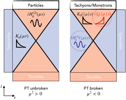
Figure 1: Schematic of the asymptotic behaviour of the propagator $\Delta(x,t)$ for large spacetime intervals inside and outside of the lightcone in the case of (left) unbroken ($\mu^{2}>0$) and (right) spontaneously broken ($\mu^{2}<0$) PT symmetry. For large timelike intervals ($i.e.$ inside the lightcone), while amplitudes asymptotically display oscillatory ($H_{0}^{(2)}$) behaviour in the PT-unbroken sector, they can display exponential growth ($I_{0}$) in the PT-broken sector, or in other words monstronic behaviour. For spacelike intervals ($i.e.$ outside the lightcone, beyond the Lieb-Robinson bound), amplitudes in the PT-broken sector asymptotically display oscillatory (tachyonic) behaviour in contrast with their exponential suppression ($K_{0}$) when PT symmetry is unbroken.

III Renormalization group analysis

It is known that the Hermitian massive Thirring model admits a continuous line of interacting massless fixed points, which is either attractive or repulsive depending on the bare mass and coupling strength. We now study the behaviour of the generalized massive Thirring model under renormalization to investigate how the occurrence of a $\gamma_{5}$-dependent mass and the interplay between interactions and non-Hermiticity modify those results. Of particular interest is the behaviour of the model under renormalization when the propagating mass is imaginary in the PT-broken sector ($\mu^{2}<0$). The renormalization group analysis detailed in Appendix B predicts the following flow equations for the mass $m_{1}$ and its $\gamma_{5}$-dependent counterpart $m_{2}$

$$\partial_{\tau}\bar{m}_{i}=\bar{m}_{i}\left[1+\frac{2\bar{\lambda}}{\pi\left(1+4\bar{\mu}^{2}\right)}\right],\quad\quad(i=1,2)$$ (8)

where $\tau$ is the ’RG time’ $|\tau|=\ln(\Lambda/k)$ and the dimensionless masses $\bar{m}_{i}=(2k)^{-1}{m}_{k,i}$ and coupling strength $\bar{\lambda}=\lambda_{k}/2$ are expressed in units of the running momentum scale $k$. The ultraviolet cutoff $\Lambda$ is naturally provided by the lattice spacing if the underlying microscopic model is defined on a lattice. Noticing the similarity between the flow equations for $m_{1}$ and $m_{2}$, one can show that the ratio between $m_{1}$ and $m_{2}$ remains constant under renormalization

$$\partial_{\tau}\left(\frac{\bar{m}_{1}}{\bar{m}_{2}}\right)=0.$$ (9)

The structure of the RG flow reflects the fact that the only physically-relevant mass in the problem (namely the one appearing in the propagator) is given by $\mu$. Accordingly, in the PT-unbroken sector, the Hamiltonian of the generalized non-Hermitian massive Thirring (1) is known to admit the same spectrum Bender et al. (2018) as that of the Hermitian massive Thirring with mass $\mu=\sqrt{m_{1}^{2}-m_{2}^{2}}$. Given these considerations, the flow equations can be expressed entirely in terms of $\bar{\mu}^{2}=\bar{m}_{1}^{2}-\bar{m}_{2}^{2}$ (whose sign is therefore also preserved under renormalization) and $\bar{\lambda}$ as

$$\tfrac{1}{2}\partial_{\tau}\bar{\mu}^{2} =\bar{\mu}^{2}\left[1+\frac{2\bar{\lambda}}{\pi\left(1+4\bar{\mu}^{2}\right)}\right],$$ (10)

$$\partial_{\tau}\bar{\lambda} =\frac{16}{\pi}\frac{\bar{\lambda}^{2}\bar{\mu}^{2}}{\left(1+4\bar{\mu}^{2}\right)^{2}}.$$

The phase diagram of the non-Hermitian Thirring model obtained from the FRG flow Eqs. (10) is reported in Fig. 2.

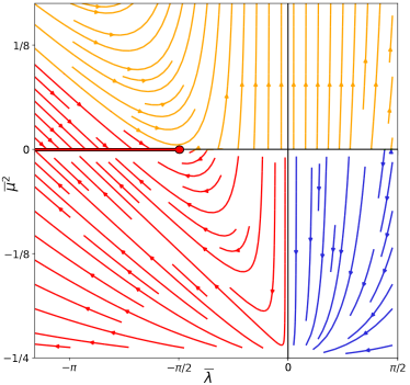
Figure 2: RG flow for the dimensionless square mass $\bar{\mu}^{2}$ and quartic coupling strength $\bar{\lambda}$. In the PT-unbroken sector ($\mu^{2}>0$), the flows qualitatively reproduce the traditional BKT picture: the line of fixed points with $\bar{\mu}^{2}=0$ that is attractive for $\bar{\lambda}\leq-\pi/2$ (red solid line) and repulsive otherwise. This results in a massless BKT (red) and a massive (yellow) phase separated by the well-known BKT point. The PT-broken sector ($\bar{\mu}^{2}<0$) displays for $\bar{\lambda}<0$ semicircular flows consistent with previous perturbative RG studies of the generalized sine-Gordon Ashida et al. (2017). In this region, the BKT line is attractive also for $-\pi/2\leq\bar{\lambda}\leq 0$, resulting in the stabilization of the power-law scaling for all attractive interaction strengths (red). For repulsive interactions $\bar{\lambda}\geq 0$, a novel massive phase emerges characterized by a finite imaginary mass and leading to exponentially-growing (monstronic) amplitudes for large timelike intervals and oscillatory (tachyonic) amplitudes for large spacelike intervals.

For $\bar{\mu}^{2}>0$ ($i.e.$ the PT-unbroken sector), the flow reproduces the well-known BKT physics: one finds a line of fixed points at $\bar{\mu}^{2}=0$ that is attractive (double red line) for $\bar{\lambda}\leq-\pi/2$ and repulsive otherwise. The unbinding point at $\bar{\lambda}=-\pi/2$ is reported as a red full circle. More interestingly, in the PT-broken sector $\bar{\mu}^{2}<0$, the flow Eqs. (10) display a spinodial line at $\bar{\mu}^{2}=-1/4$, where both beta functions become infinite. This spinodal line represents the UV limit of the theory. For each point above this line $\bar{\mu}^{2}>-1/4$ with $\bar{\lambda}<0$, the flows are semicircular and the system will eventually end up in any of the attractive BKT fixed points. In this regime, the behaviour of the non-Hermitian Thirring model reproduces the one of the generalized sine-Gordon model Ashida et al. (2017), as expected from duality arguments Coleman (1975a).

This analogy fails when the fermions, representing the sine-Gordon solitons, become repulsive, $i.e.$ when $\bar{\lambda}>0$. While the PT-unbroken sector displays the same infrared behaviour for any $\bar{\lambda}>-\pi/2$ (yellow region in Fig. 2), a novel infrared phase emerges in the PT-broken sector of the massive Thirring model for $\bar{\lambda}>0$ (blue region in Fig. 2). There, the flow is attracted to an infrared spinodal point $(\bar{\mu}^{2},\bar{\lambda})=(-1/4,0)$, which is the termination of the UV spinodal line described for $\bar{\lambda}<0$. This point corresponds to a non-interacting theory with an imaginary propagating mass ($\bar{\mu}^{2}=-1/4$). Yet, the spinodal nature of this attractive infrared point causes the flow to terminate at a finite scale $k_{c}$ in its vicinity Nagy (2012). The spinodal point stemming from the singularity in the beta functions is also known to arise in Hermitian systems. In Hermitian systems, $k_{c}$ represents a finite correlation lengthscale of the system and the value of the couplings at the breakdown of the flow coincide with the thermodynamic properties of the system in the massive infrared phase Nagy (2012). These effective parameters describing the renormalized theory are non-universal and depend on the microscopic (bare) initial conditions of the flow. Therefore, the spinodal infrared point describes a non-critical massive phase.

At $\bar{\lambda}=0$, a phase transition occurs between a massless (interacting) phase and a phase with an imaginary propagating mass. As explained above, this phase is characterized by tachyonic modes. Since the flows interrupt before reaching the singularity, the renormalized (imaginary) mass depends on the microscopic parameters of the model, providing a way to tune the corresponding mode oscillation/amplification rate. We mention that an infrared phase was evidenced in the non-perturbative treatment of the non-Hermitian sine-Gordon model. There, the semi-circular flows occurring in the PT-broken phase break down at a finite value of the superfluid stiffness $K$, where a new infrared phase appears Ashida (2020). Whereas this phase has found no clear interpretation in the sine-Gordon paradigm, the fermionic Thirring picture provides a physical meaning for this phase as a truly non-Hermitian phase hosting tachyonic excitations occurring when the interaction between the fermions (the solitons of the sine-Gordon model Coleman (1975b)) becomes repulsive in the PT-broken sector. In the following we will show how the transparency of the Thirring picture allows us to generalize our findings to the presence of external gauge fields.

IV Generalized massive Thirring with external gauge-field

We now study the influence of an additional external gauge-field on the phase diagram of the generalized massive Thirring model, with particular focus on the interplay between such interactions and spontaneous symmetry breaking of PT symmetry. As mentionned before, these terms may be used to model various phenomena depending on the setting such as incommensurabilities in classical systems Pokrovsky and Talapov (1979); Puga et al. (1982), magnetic fields in spin systems Chitra and Giamarchi (1997) soliton fugacities Horovitz et al. (1983) in bosonic settings or chemical potentials Schulz (1980) in fermionic systems. The modified Hamiltonian obtained via the minimal substitution $\partial_{\mu}\rightarrow D_{\mu}=\partial_{\mu}-id_{\mu}$ with $d_{0}=d$ and $d_{1}=0$ reads

$$H=\int dx\left[\bar{\psi}\left(-i\not{\nabla}+d\gamma_{0}+{m}_{1}+{m}_{2}\gamma_{5}\right)\psi+\lambda(\bar{\psi}\psi)^{2}\right].$$ (11)

We first note that $\mu^{2}=m_{1}^{2}-m_{2}^{2}$ remains the effective mass even when $d\neq 0$ (this can be checked by writing the field equations of motion for the gauged-transformed fermions $\tilde{\psi}\equiv e^{id^{\mu}x_{\mu}}\psi$). The RG flow reflects this fact and (9) remains unchanged. The associated flow equations derived in Appendix B can again be expressed in terms of $\bar{\mu}^{2}$

$$\tfrac{1}{2}\partial_{\tau}\bar{\mu}^{2} =\bar{\mu}^{2}\left(1+\frac{\bar{\lambda}}{4\pi\bar{d}^{2}}\frac{\left(1-4\bar{d}^{2}+4\bar{\mu}^{2}\right)}{\sqrt{\left[2\left(\frac{1-4\bar{d}^{2}+4\bar{\mu}^{2}}{4\bar{d}}\right)^{2}+1\right]^{2}-1}}\right),$$ (12)

$$\tfrac{1}{2}\partial_{\tau}\bar{d}^{2} =\bar{d}^{2}-\frac{\bar{\lambda}}{4\pi}$$

$$+ \frac{\bar{\lambda}}{4\pi}\frac{\left(1-4\bar{d}^{2}+4\bar{\mu}^{2}\right)\left(1+\frac{1}{8\bar{d}^{2}}\left[1-4\bar{d}^{2}+4\bar{\mu}^{2}\right]\right)}{\sqrt{\left[2\left(\frac{1-4\bar{d}^{2}+4\bar{\mu}^{2}}{4\bar{d}}\right)^{2}+1\right]^{2}-1}},$$

$$\partial_{\tau}\bar{\lambda} =-\frac{2\bar{\lambda}^{2}}{\pi}\left(1-\frac{\bar{\mu}^{2}}{\bar{d}^{2}}\right)\frac{1}{\sqrt{\left[2\left(\frac{1-4\bar{d}^{2}+4\bar{\mu}^{2}}{4\bar{d}}\right)^{2}+1\right]^{2}-1}}.$$

The flow diagram for the following combination of couplings $(\bar{\mu}^{2}-\bar{d}^{2},\bar{\lambda})$ is displayed in Fig. 3.

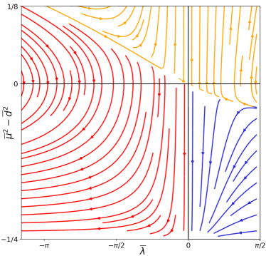
Figure 3: RG flow slice for the coupling combination $\bar{\mu}^{2}-\bar{d}^{2}$ and the quartic coupling strength $\bar{\lambda}$ (for $\bar{d}$ fixed at $0.3$, other values of $\bar{d}$ lead to qualitatively equivalent flow charts). In particular, the flow no longer displays $\bar{\mu}^{2}=0$ as a continuum of fixed points for $\bar{d}\neq 0$, effectively ruling out the BKT transition as pointed out in a recent study Nosov et al. (2017). For points belonging to a region (in blue) included in the lower-left quadrant ($\bar{\lambda}>0$ and $\bar{\mu}^{2}<d^{2}$), the flows converge to $\bar{\mu}^{2}-\bar{d}^{2}=-1/4$ and $\bar{\lambda}=0$. This includes the PT-broken sector for which $\bar{\mu}^{2}<0$ and a part of of the PT-unbroken sector $\bar{\mu}^{2}>0$.

Comparing Figs. 2 and 3, we see that the flow lines are strongly modified by the gauge-field. As a notable feature, for $d\neq 0$, the flow equations no longer display $\bar{\mu}^{2}=0$ as a continuum line of fixed points (parametrized by the interaction $\bar{\lambda}$), effectively ruling out the BKT transition. This is consistent with a recent study focusing on the Hermitian model Nosov et al. (2017). Instead, the trajectories in red in Fig. 3 flow towards increasingly strong attractive interactions $\bar{\lambda}<0$. Note that for $\bar{\lambda}\ll 0$, $\bar{\mu}^{2}$ and the corresponding beta function $\partial_{t}\bar{\mu}^{2}$ have opposite signs, as can be inferred from (12). Hence, the trajectories in the lower left sector of the phase diagram in Fig. 3 converge towards $\bar{\mu}^{2}=0$. Thus, while the original gapless BKT phase (in red in Fig. 2) is lost in the presence of external gauge fields, the corresponding phase at finite $d$ (in red in Fig. 3) remains massless nonetheless.

As shown in Fig. 3, the point $(\bar{\mu}^{2}-\bar{d}^{2},\bar{\lambda})=(-1/4,0)$ has a basin of attraction contained in the region defined by ${\bar{\lambda}}>0$ and $\bar{\mu}^{2}<\bar{d}^{2}$ (the lower-left quadrant). This includes the PT-broken sector for which $\bar{\mu}^{2}<0$ and a part of the PT-unbroken sector $\bar{\mu}^{2}>0$. In contrast to the BKT phase which is wiped out by the gauge field, the new tachyonic phase is preserved. Furthermore, since the renormalized theory is only subject to the constraint $\bar{\mu}^{2}-\bar{d}^{2}=-1/4$, the renormalized mass itself can be continuously tuned via the bare parameters $\bar{\mu}_{0}$, $\bar{d}_{0}$ and $\bar{\lambda}_{0}$. This is demonstrated in Fig. 4 which displays the flow of $\bar{\mu}^{2}$, $\bar{d}^{2}$ and $\bar{\mu}^{2}-\bar{d}^{2}$ together with $\bar{\lambda}$ for different starting points (solid black dots) corresponding to distinct bare values of the coupling strengths.

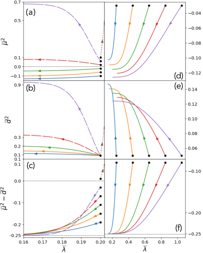
Figure 4: Flow diagrams for the dimensionless propagating mass $\bar{\mu}^{2}$, external gauge field $\bar{d}^{2}$ as well as the combination $\bar{\mu}^{2}-\bar{d}^{2}$ together with $\bar{\lambda}$ for different initial conditions obtained by varying the bare value of the mass $\bar{\mu}_{0}^{2}$ in panels (a), (b) and (c) or by tuning the strength of the bare interaction $\bar{\lambda}_{0}$ in the region of positive $\bar{\lambda}$ in panels (d), (e) and (f). Unless the initial value for $\bar{\mu}^{2}-\bar{d}^{2}$ is above a given threshold (dotted trajectories), $\bar{\lambda}$ is irrelevant and $\bar{\mu}^{2}-\bar{d}^{2}$ converges towards $-1/4$. For all trajectories in this regime, one observes that different bare conditions lead to different values of the renormalized square mass $\bar{\mu}^{2}$, to which $\bar{d}^{2}$ adapts since the renormalized difference is constrained. This is the case for the region of the PT-unbroken ($\bar{\mu}^{2}>0$) sector in the aforementioned regime (dashed lines) and for the PT-broken sector (solid lines). The renormalized propagating mass can therefore be tuned through the microscopic (bare) parameters of the model.

We first focus on the panels (a), (b) and (c) in Fig. 4, which displays the flows of $\bar{\mu}^{2}$, $\bar{d}^{2}$ and $\bar{\mu}^{2}-\bar{d}^{2}$, respectively, as a function of $\bar{\lambda}$ for different initial (bare) values of the propagating mass $\bar{\mu}_{0}$. The bare values of the gauge field $\bar{d}_{0}$ and coupling $\bar{\lambda}_{0}$ are kept fixed. Three different regimes are identified, corresponding respectively to the dotted, dashed and solid flow lines. In panel (c), there exists a threshold value $\bar{\mu}^{2}_{0}-\bar{d}^{2}_{0}\approx 0$ for the bare difference in coupling strengths above which both $\bar{\lambda}$ and $\bar{\mu}^{2}-\bar{d}^{2}$ flow towards arbitrary high values (dotted curve). In this regime, both $\bar{\mu}$ and $\bar{d}$ diverge (see panels (a) and (b)). This phase corresponds to the yellow region in the upper right ($\bar{\lambda}>0$) quadrant in Fig. 3. In contrast, below this threshold, we have flows which converge to $\bar{\mu}^{2}-\bar{d}^{2}=-1/4$ and $\bar{\lambda}=0$ (dashed and solid lines in panel (c)). This corresponds to the blue region in the lower right quadrant ($\bar{\lambda}>0$) in Fig. 3. From panel (a), we infer that these trajectories arise in both the unbroken PT sector (dashed lines) where $\bar{\mu}^{2}>0$ and the PT-broken sector (solid lines) where $\bar{\mu}^{2}<0$. In both cases, each value of the bare mass $\bar{\mu}_{0}^{2}$ (solid black dots) leads to a different value of the renormalized mass $\bar{\mu}^{2}$. The value of $\bar{d}^{2}$ for the dashed and solid trajectories adapts correspondingly, see panel (b), so that $\bar{\mu}^{2}-\bar{d}^{2}\to-1/4$ as displayed in panel (c).

Panels (d), (e) and (f) show the flows of $\bar{\mu}^{2}$, $\bar{d}^{2}$ and $\bar{\mu}^{2}-\bar{d}^{2}$ as a function of $\bar{\lambda}$ for different initial (bare) values $\bar{\lambda}_{0}$ of the quartic coupling strength. The bare values $\bar{d}_{0},\bar{\mu}_{0}$ are kept fixed and chosen in the PT-broken sector ($\bar{\mu}^{2}<0$) so that the trajectories belong to the blue region in FIG. 4. As shown in panel (d), each value of the bare coupling strength $\bar{\lambda}_{0}$ (solid black dots) leads to a different value of the renormalized mass $\bar{\mu}^{2}$. Once again, $\bar{d}$ adapts, see panel (e), so that $\bar{\mu}^{2}-\bar{d}^{2}\to-1/4$ asymptotically as shown in panel (f). To summarize, we see that the renormalized mass and the corresponding asymptotic properties of the propagator can be tuned via the bare parameters of the model ($\bar{\mu}_{0}$, $\bar{d}_{0}$, $\bar{\lambda}_{0}$). In particular, one can tune in the PT-broken sector the amplification/oscillation rate of amplitudes of the tachyonic modes. We note that this applies to a part of the PT-unbroken sector in which the (now real) mass of the particle modes can be tuned as well.

V Conclusion/Discussion.

The functional renormalization-group was employed to investigate putative phase transitions and the influence of external gauge fields in a generalized PT-symmetric two-dimensional massive Thirring model. We see that this model spontaneously breaks PT symmetry in a certain coupling regime. We find that for attractive interactions, PT symmetry is restored in the asymptotic flow. However, for repulsive interactions, our analysis predicts a novel PT-broken phase, which manifests as an attractive spinodal fixed point of the flow equations, characterized by the termination of the flow at a finite non-zero momentum $k_{c}$. This phase harbours an imaginary mass describing tachyonic  excitations, which display exponentially (oscillatory) amplitudes for timelike (spacelike) intervals and potentially violate Lieb-Robinson bounds.

The presence of an additional gauge field is shown to dramatically alter the renormalization group flows. The tachyonic PT-broken phase is however robust to this gauge field. As opposed to standard massive phases, the renormalized imaginary mass of the tachyons can be tuned in a controlled manner via the microscopic parameters.

Future perspectives include the quantitative study of the relation between the generalized Thirring model and the PT-broken sine-Gordon model Ashida (2020), generalizing the duality argument to the non-Hermitian setting Coleman (1975a). Other possible enlightening perspectives might include the computation of the mass of lowest excitation as a function of the interaction strength in the PT-symmetric Thirring/sine-Gordon models, aiming to generalize previous results based on the derivative expansion in the Hermitian setting Daviet and Dupuis (2019) to the PT-broken regime. Lastly, it would be exciting to explore prospects for realizing such novel monstronic/tachyonic modes stemming from PT symmetry breaking in realistic experimental platforms which can simulate non-Hermitian Hamiltonians such as ultracold atoms and exciton-polariton condensates Takasu et al. (2020); Barontini et al. (2013); Brennecke et al. (2013); Ashida and Ueda (2015); Gao et al. (2015); Klinder et al. (2015); El-Ganainy et al. (2018); Zeuner et al. (2015); Rüter et al. (2010).

Appendix A Tachyonic propagator in the PT-broken phase.

Whether PT symmetry is spontaneously broken (or equivalently the sign of the square propagating mass $\mu^{2}$) is crucial to determine the asymptotic decay of propagators. A standard calculation in the PT-symmetric case ($\mu^{2}>0$) leads to asymptotic properties of amplitudes analogous to the purely Hermitian case: equation (6) only differs from the Hermitian case through the substitution $\mu\rightarrow m_{1}$. In contrast, we will see that PT symmetry breaking ($\mu^{2}>0$) has dramatic consequences for the asymptotic decay of propagators. The fermion propagator can be generally obtained as follows

$$-i\Delta_{F}(x,t)=(i\not{\partial}-m_{1}-m_{2}\gamma_{5})\Delta(x,t),\mbox{ where }\Delta(x,t)\equiv\int\frac{d^{2}k}{(2\pi)^{2}}\frac{ie^{-ik^{\mu}x_{\mu}}}{k^{2}-\mu^{2}+i\epsilon},$$ (13)

in which $\epsilon\rightarrow 0^{+}$. In the PT-broken phase, the propagating mass $\mu$ becomes imaginary $\mu=i|\mu|$. We now derive a closed form for $\Delta(x,t)$ in this particular case:

$$\Delta(x,t) =\int\frac{d^{2}k}{(2\pi)^{2}}\frac{ie^{-ik^{\mu}x_{\mu}}}{k^{2}+|\mu|^{2}+i\epsilon}$$ (14)

$$=\int\frac{dk_{1}dk_{0}}{(2\pi)^{2}}\frac{ie^{-ik_{0}t+i{k}_{1}{x}}}{k^{2}_{0}-k_{1}^{2}+\mu^{2}+i\epsilon}$$

$$=i\int_{|{k}_{1}|<|\mu|}\frac{d{k}_{1}}{(2\pi)}\frac{e^{-\sqrt{|\mu|^{2}-k_{1}^{2}}|t|}}{2\sqrt{|\mu|^{2}-k_{1}^{2}}}e^{+i{k}_{1}{x}}+\int_{|{k}_{1}|>|\mu|}\frac{d{k}_{1}}{(2\pi)}\frac{e^{-i\sqrt{k_{1}^{2}-|\mu|^{2}}|t|}}{2\sqrt{k_{1}^{2}-|\mu|^{2}}}e^{+i{k}_{1}{x}}$$

$$=i\int_{0}^{|\mu|}\frac{d{k}_{1}}{(2\pi)}\frac{e^{-\sqrt{|\mu|^{2}-k_{1}^{2}}|t|}}{\sqrt{|\mu|^{2}-k_{1}^{2}}}\cos(k_{1}x)+\int_{|\mu|}^{\infty}\frac{d{k}_{1}}{(2\pi)}\frac{e^{-i\sqrt{k_{1}^{2}-|\mu|^{2}}|t|}}{\sqrt{k_{1}^{2}-|\mu|^{2}}}\cos(k_{1}x),$$

in which we have evaluated the integral in $k_{0}$ as follows:

$$\int_{-\infty}^{+\infty}\frac{dk_{0}}{2\pi}\frac{ie^{-ik_{0}t}}{{k^{2}_{0}-k_{1}^{2}+\mu^{2}+i\epsilon}}=\frac{e^{-i\sqrt{k_{1}^{2}-|\mu|^{2}}|t|}}{2\sqrt{k_{1}^{2}-|\mu|^{2}}}\theta(k_{1}^{2}-|\mu|^{2})+\frac{e^{-\sqrt{|\mu|^{2}-k_{1}^{2}}|t|}}{-2i\sqrt{|\mu|^{2}-k_{1}^{2}}}\theta(|\mu|^{2}-k_{1}^{2}),$$ (15)

taking into account the fact that for $|k_{1}|>|\mu|$, the poles are on the real axis at $k_{0}=\pm\sqrt{k_{1}^{2}-|\mu|^{2}}$ while for $|k_{1}|<|\mu|$, they are on the imaginary axis at $k_{0}=\pm i\sqrt{|\mu|^{2}-k_{1}^{2}}$. For spacelike intervals, we can pick a frame of reference such that the spacetime interval is purely spatial and revert back to the original coordinates to find

$$\Delta(x,t) =i\int_{0}^{\mu}\frac{d{k}_{1}}{(2\pi)}\frac{\cos(k_{1}r)}{\sqrt{|\mu|^{2}-k_{1}^{2}}}+\int_{\mu}^{\infty}\frac{d{k}_{1}}{(2\pi)}\frac{\cos(k_{1}r)}{\sqrt{k_{1}^{2}-|\mu|^{2}}}$$

$$=\frac{i}{4}J_{0}(|\mu|r)-\frac{1}{4}Y_{0}(|\mu|r)$$

$$=\frac{i}{4}H_{0}(|\mu|r),$$

where $r=\sqrt{-t^{2}+x^{2}}$. Similarly for timelike intervals, we can write

$$\Delta(x,t) =i\int_{0}^{|\mu|}\frac{d{k}_{1}}{(2\pi)}\frac{e^{-\sqrt{|\mu|^{2}-k_{1}^{2}}s}}{\sqrt{|\mu|^{2}-k_{1}^{2}}}+\int_{{|\mu|}}^{\infty}\frac{d{k}_{1}}{(2\pi)}\frac{e^{-i\sqrt{k_{1}^{2}-|\mu|^{2}}s}}{\sqrt{k_{1}^{2}-|\mu|^{2}}}$$ (16)

$$=i\int_{0}^{|\mu|}\frac{dp}{(2\pi)}\frac{e^{-ps}}{\sqrt{|\mu|^{2}-p^{2}}}+\int_{{|\mu|}}^{\infty}\frac{dl}{(2\pi)}\frac{e^{-ils}}{\sqrt{l^{2}+|\mu|^{2}}}$$

$$=\frac{i}{2}I_{0}(|\mu|s)+\frac{1}{2\pi}K(|\mu|s),$$

where $s=\sqrt{+t^{2}-x^{2}}$. Note that the fact that the presence of the Bessel function $I_{0}(|\mu|s)$ implies exponential growth of amplitudes with time. This intrinsically violates unitarity of dynamics, which is generally assumed. This apparent problem is sometimes cured through the instauration of an infrared cutoff for $k_{1}$ at $|\mu|$. Perepelitsa (2016) In the non-Hermitian setting, these cannot however be excluded, particularly in the PT-broken phase where unitarity cannot be restored through a choice of scalar product. Bender et al. (2018)

Appendix B Derivation of the flow equations.

Summary. The flow equations (12) are derived from the Wetterich equation based on a LPA scheme coupled with an expansion in the field-dependent part of the inverse regularized propagator applied onto the euclidean action corresponding to the generalized massive Thirring Hamiltonian in the presence of an external gauge field (11). Equations (12) reduce to (10) for $d=0$. The sharp cutoff $r\left(\frac{q^{2}}{k^{2}}\right)=\left\{\begin{array}[]{cc}\infty,&q^{2}<k^{2}\\ 0,&q^{2}>k^{2}\end{array}\right.$ is employed, which facilitates explicit evaluation of the threshold functions. Details of the calculation are provided below and closely follow the FRG treatment of the Hermitian massive Thirring model in the presence of external gauge fields Nosov et al. (2017) while generalizing them to the non-Hermitian case. In particular, the computation differs in the additional presence of a $\gamma_{5}$-dependent mass term $\gamma_{5}m_{2}$ with ${\gamma_{5}=\sigma_{3}}$.

Euclidean action. We start by writing the Euclidean action corresponding to the Hamiltonian (11) for the two-dimensional massive Thirring model in the presence of external gauge fields :

$$S=i\int d^{2}r\left[\bar{\psi}\left(\sigma_{\mu}D_{\mu}+m_{1}+m_{2}\sigma_{3}\right)\psi+\lambda(\bar{\psi}\psi)^{2}\right],$$ (17)

where the covariant derivative $D_{\mu}=\partial_{\mu}-d\delta_{\mu,1}$ is given in terms of the external gauge field $d$. Through a Fourier transform

$$\psi(\mathbf{x})=\int\frac{d^{2}\mathbf{p}}{(2\pi)^{2}}e^{i\mathbf{px}}\psi_{\mathbf{p}}\equiv\int_{p}e^{i\mathbf{px}}\psi_{\mathbf{p}},$$ (18)

the action (17) can be written as follows in momentum space

$${S}= \int\frac{d^{2}\mathbf{p}}{(2\pi)^{2}}\bar{\psi}_{\mathbf{p}}(-\not{p}-i\not{d}+i{m}_{1}+im_{2}\sigma_{3})\psi_{\mathbf{p}}+(2\pi)^{2}\lambda$$ (19)

$$\times\int\prod_{i=1}^{4}\frac{d^{2}\mathbf{p}_{i}}{(2\pi)^{2}}\left(\bar{\psi}_{\mathbf{p}_{1}}\psi_{\mathbf{p}_{2}}\right)\left(\bar{\psi}_{\mathbf{p}_{3}}\psi_{\mathbf{p}_{4}}\right)$$

$$\times\delta\left(-\mathbf{p}_{\mathbf{1}}+\mathbf{p}_{\mathbf{2}}-\mathbf{p}_{\mathbf{3}}+\mathbf{p}_{\mathbf{4}}\right),$$

where the (newly redefined) slashed notations $\not{p}=p_{\mu}\sigma_{\mu},\not{d}=d\sigma_{1}$ are used.

FRG. Wetterich’s formulation of RG is based on the effective average action $\Gamma_{k}$, a generalization of the effective action including only rapidly-oscillating modes, namely fluctuations with wavevectors satisfying $q^{2}\geqslant k^{2}$, where $k$ is a UV for slow modes Wetterich (1993b). This is implemented through the use of a regulator (IR cutoff) $R_{k}$ in the inverse propagator. The regulator decouples slowly oscillating modes with momenta $q^{2}\leqslant k^{2}$ by largely increasing their mass, while high momentum modes remain unaffected.

The Wetterich equation governs how $\Gamma_{k}$ depends on the scale $k$

$$\partial_{k}\Gamma_{k}=-\frac{1}{2}\operatorname{Tr}\left[\frac{\partial_{k}R_{k}}{\Gamma^{(2)}+R_{k}}\right]=-\frac{1}{2}\tilde{\partial}_{k}\operatorname{Tr}\log\left(\Gamma^{(2)}+R_{k}\right),$$ (20)

with $\Gamma^{(2)}$ denoting the second functional derivative of $\Gamma_{k}$ with respect to the fields. The trace is here meant as both an integration over momenta as well as a sum over internal indices. The tilde on the derivative $\tilde{\partial}_{k}$ is intended as a sign that it acts only on the $k$-dependence of the regulator $R_{k}$ and not on that of $\Gamma^{(2)}$. The minus sign on the right-hand side of Eq. (20) is due to the Grassman nature of the fields $\bar{\psi}$ and $\psi$ Berges et al. (2002b).

Effective action. By definition, for $k=0$, the average action is identical to the effective action, as the IR cutoff is not present and all modes are included. Similarly to (19) the effective action is defined as

$$\Gamma_{k}= \int\frac{d^{2}\mathbf{p}}{(2\pi)^{2}}\bar{\psi}_{\mathbf{p}}\left(-\not{p}-i\not{d}_{k}+i{m}_{1,k}+i{m}_{2,k}\sigma_{3}\right)\psi_{\mathbf{p}}+(2\pi)^{2}$$ (21)

$$\times\lambda_{k}\int\prod_{i=1}^{4}\frac{d^{2}\mathbf{p}_{i}}{(2\pi)^{2}}\left(\bar{\psi}_{\mathbf{p}_{1}}\psi_{\mathbf{p}_{2}}\right)\left(\bar{\psi}_{\mathbf{p}_{3}}\psi_{\mathbf{p}_{4}}\right)$$

$$\times\delta\left(-\mathbf{p}_{1}+\mathbf{p}_{2}-\mathbf{p}_{3}+\mathbf{p}_{4}\right),$$

where the momentum-scale index $k$ indicated the scale-dependence of all parameters in the effective action.

Regularized propagator expansion in the field-dependent part. Using Eq. (20), the effects of the interaction $\lambda$ on the various parameters and in particular their flows and fixed points can be studied systematically. To be able to make analytical predictions, one may split the inverse regularized propagator into the field-independent $\left(\Gamma_{k,0}^{(2)}+R_{k}\right)$ and the field-dependent $\left(\Delta\Gamma_{k}^{(2)}\right)$ parts, which yields

$$\frac{\partial_{k}R_{k}}{\Gamma^{(2)}+R_{k}}= \tilde{\partial}_{k}\log\left(\Gamma_{k,0}^{(2)}+\Delta\Gamma_{k}^{(2)}+R_{k}\right)$$ (22)

$$= \tilde{\partial}_{k}\log\left(\Gamma_{k,0}^{(2)}+R_{k}\right)+\tilde{\partial}_{k}\frac{\Delta\Gamma_{k}^{(2)}}{\Gamma_{k,0}^{(2)}+R_{k}}$$

$$-\frac{1}{2}\tilde{\partial}_{k}\left(\frac{\Delta\Gamma_{k}^{(2)}}{\Gamma_{k,0}^{(2)}+R_{k}}\right)^{2}+\cdots$$

Regulator. The regulator may be chosen as Gies and Janssen (2010); Braun (2012)

$$R_{k}=-\frac{\delta_{p,q}}{(2\pi)^{2}}r\left(\frac{q^{2}}{k^{2}}\right)\left(\begin{array}[]{cc}0&\not{q}^{T}\\ \not{q}&0\end{array}\right)$$ (23)

for Thirring fermions. We now compute explicitly the field-independent part of the inverse (regularized) propagator and the corresponding field-dependent part.

Inverse propagator computation. The matrix of second derivatives of $\Gamma_{k}$ with respect to the fermionic fields can be obtained from Eq. (21):

$$\Gamma_{k}^{(2)}(p,q)=\left(\begin{array}[]{ll}\vec{\partial}_{\psi_{-p}^{T}}\Gamma_{k}\overleftarrow{\partial}_{\psi_{q}}&\vec{\partial}_{\psi_{-p}^{T}}\Gamma_{k}\overleftarrow{\partial}_{\bar{\psi}_{-q}^{T}}\\ \vec{\partial}_{\bar{\psi}_{p}}\Gamma_{k}\overleftarrow{\partial}_{\psi_{q}}&\vec{\partial}_{\bar{\psi}_{p}}\Gamma_{k}\overleftarrow{\partial}_{\bar{\psi}_{-q}^{T}}\end{array}\right),$$ (24)

which yields the field-independent part

$$\Gamma_{k,0}^{(2)}(p,q)=\frac{\delta_{p,q}}{(2\pi)^{2}}\left(\begin{array}[]{cc}0&-\not{p}^{T}+i\not{d}^{T}-i{m}_{1,k}{-im_{2,k}\sigma_{3}}\\ -\not{p}-i\not{d}+i{m}_{1,k}{+im_{2,k}\sigma_{3}}&0\end{array}\right).$$ (25)

The inverted regularized propagator therefore reads

$$\frac{\left(\Gamma_{k,0}^{(2)}+R_{k}\right)_{(p,q)}}{\frac{\delta_{p,q}}{(2\pi)^{2}}}=\left(\begin{array}[]{cc}0&-\not{p}^{T}\left[1+r\left(\frac{q^{2}}{k^{2}}\right)\right]+i\not{d}^{T}-i{m}_{1,k}{-im_{2,k}\sigma_{3}}\\ -\not{p}\left[1+r\left(\frac{q^{2}}{k^{2}}\right)\right]-i\not{d}+i{m}_{1,k}{+im_{2,k}\sigma_{3}}&0\end{array}\right),$$ (26)

the inverse of the matrix yields the result (29). To find the form of the field-dependent part (25) the property $\bar{\psi}\psi=-\psi^{T}\bar{\psi}^{T}$ appears to be useful.

If $B$ and $C$ are invertible matrices, we have that

$$\left[\begin{array}[]{cc}0&B\\ C&0\end{array}\right]^{-1}=\left[\begin{array}[]{cc}0&C^{-1}\\ B^{-1}&0\end{array}\right],$$ (27)

which we can apply to the inverted regularized propagator together with inversion of linear combinations of sigma matrices

$$(z_{0}\sigma_{0}+z_{1}\sigma_{1}+z_{2}\sigma_{2}+z_{3}\sigma_{3})^{-1}=\frac{z_{0}\sigma_{0}-z_{1}\sigma_{1}-z_{2}\sigma_{2}-z_{3}\sigma_{3}}{z_{0}^{2}-z_{1}^{2}-z_{2}^{2}-z_{3}^{2}},$$ (28)

provided that $z_{0}^{2}-z_{1}^{2}-z_{2}^{2}-z_{3}^{2}\neq 0$. Using those identities, the propagator is found to be

$$\left(\Gamma_{k,0}^{(2)}+R_{k}\right)^{-1}=(2\pi)^{2}\delta_{p,q}\left(\begin{array}[]{cc}0&\frac{\not{\alpha}_{k}-i{m}_{1,k}{+im_{2,k}}}{\alpha_{k}^{2}+\mu_{k}^{2}}\\ \frac{\not{\beta}_{k}^{T}+i{m}_{1,k}{-im_{2,k}}}{\beta_{k}^{2}+\mu_{k}^{2}}&0\end{array}\right)=(2\pi)^{2}\hat{G}_{0}\delta_{p,q},$$ (29)

where $\not{\alpha}_{k}=-\not{q}\left[1+r\left(\frac{q^{2}}{k^{2}}\right)\right]-i\not{d}_{k}\equiv a_{k}\not{q}-i\not{d}_{k}$ and $\not{\beta}_{k}=$ $-\not{q}\left[1+r\left(\frac{q^{2}}{k^{2}}\right)\right]+i\not{d}_{k}\equiv a_{k}\not{q}+i\not{d}_{k};\quad\alpha^{2}=\alpha_{1}^{2}+\alpha_{2}^{2}\quad$ and $\beta^{2}=\beta_{1}^{2}+\beta_{2}^{2}$ and $\mu_{k}^{2}\equiv m_{1,k}^{2}-m_{2,k}^{2}$.

Computation of the field-dependent part of the propagator. The field-dependent part of the propagator $\Delta\Gamma_{k}^{(2)}\propto\lambda_{k}G_{1}$ remains unchanged with respect to the Hermitian case, namely directly follows the computation in Nosov et al. (2017). We directly obtain

$$\Delta\Gamma_{k}^{(2)}= 2(2\pi)^{2}\lambda_{k}$$ (30)

$$\times\left(\begin{array}[]{cc}-\bar{\psi}^{T}\bar{\psi}&\bar{\psi}^{T}\psi^{T}+\psi^{T}\bar{\psi}^{T}\\ \psi\bar{\psi}+\bar{\psi}\psi&-\psi\psi^{T}\end{array}\right)\delta_{p,q}$$

$$= 2(2\pi)^{2}\lambda_{k}\hat{G}_{1}\delta_{p,q},$$

where the derivative is evaluated at constant background fields. this means that $\Delta\Gamma_{k}^{(2)}$ is evaluated in momentum space at $\psi_{\mathbf{p}}=(2\pi)^{2}\psi\delta(\mathbf{p})$ and $\psi(\bar{\psi})$ on the right-hand side are constants Braun (2012).

Flow equation expansion. By combining Eqs. (20) and (26), we now expand the flow equation in powers of the fields :

$$\partial_{k}\Gamma_{k}= -\frac{1}{2}\operatorname{Tr}\left[\tilde{\partial}_{k}\log\left(\Gamma_{k,0}^{(2)}+R_{k}\right)\right]-\frac{1}{2}\operatorname{Tr}\left[\tilde{\partial}_{k}\frac{\Delta\Gamma_{k}^{(2)}}{\Gamma_{k,0}^{(2)}+R_{k}}\right]$$ (31)

$$+\frac{1}{4}\operatorname{Tr}\left[\tilde{\partial}_{k}\left(\frac{\Delta\Gamma_{k}^{(2)}}{\Gamma_{k,0}^{(2)}+R_{k}}\right)^{2}\right]+\cdots$$

The beta functions for the various coupling strengths may be obtained by comparing the coefficients of each fermion monomial of the right-hand side of Eq. (31) with the coupling terms included in the anzatz (21). We now compute the beta functions for the two-fermion and four-fermion terms in Eq. (31).

Two-fermion beta function. We focus here on the RG flow equations for the coupling strengths appearing in the quadratic part of the action. The only term contributing in the expansion (31) is given by

$$-\frac{1}{2}\operatorname{Tr}\left[\frac{\Delta\Gamma_{k}^{(2)}}{\Gamma_{k,0}^{(2)}+R_{k}}\right]=-\lambda_{k}\Omega\int\frac{d^{2}q}{(2\pi)^{2}}\operatorname{Tr}\left[\hat{G}_{1}\hat{G}_{0}\right],$$ (32)

where $\Omega$ is the volume of the system and $\hat{G}_{1}$ is defined in Eq. (30). Using $\mathrm{Tr}(\psi\bar{\psi}A)=-(\bar{\psi}A\psi)$ valid for Grassmann fields and some algebra, we compute

$$\operatorname{Tr}\left[\hat{G}_{1}\hat{G}_{0}\right]= -\frac{\alpha_{k\mu}}{\alpha_{k}^{2}+\mu_{k}^{2}}\left(\bar{\psi}\sigma_{\mu}\psi\right)+\frac{\beta_{k\mu}}{\beta_{k}^{2}+\mu_{k}^{2}}\left(\bar{\psi}\sigma_{\mu}\psi\right)+\left(\frac{1}{\alpha_{k}^{2}+\mu_{k}^{2}}+\frac{1}{\beta_{k}^{2}+\mu_{k}^{2}}\right)(-i{m}_{1,k}(\bar{\psi}\psi){-i{m}_{2,k}(\bar{\psi}\sigma_{3}\psi)})$$ (33)

$$= -2i{m}_{1,k}\frac{a_{k}^{2}q^{2}-d_{k}^{2}+\mu_{k}^{2}}{\left(a_{k}^{2}q^{2}-d_{k}^{2}+\mu_{k}^{2}\right)^{2}+4a_{k}^{2}d_{k}^{2}q_{1}^{2}}(\bar{\psi}\psi)+2id_{k}\frac{a_{k}^{2}q^{2}-d_{k}^{2}+\mu_{k}^{2}-2a_{k}^{2}q_{1}^{2}}{\left(a_{k}^{2}q^{2}-d_{k}^{2}+\mu_{k}^{2}\right)^{2}+4a_{k}^{2}d_{k}^{2}q_{1}^{2}}\left(\bar{\psi}\sigma_{1}\psi\right)$$

$$-4id_{k}\frac{a_{k}^{2}q_{1}q_{2}}{\left(a_{k}^{2}q^{2}-d_{k}^{2}+\mu_{k}^{2}\right)^{2}+4a_{k}^{2}d_{k}^{2}q_{1}^{2}}\left(\bar{\psi}\sigma_{2}\psi\right){-2i{m}_{2,k}\frac{a_{k}^{2}q^{2}-d_{k}^{2}+\mu_{k}^{2}}{\left(a_{k}^{2}q^{2}-d_{k}^{2}+\mu_{k}^{2}\right)^{2}+4a_{k}^{2}d_{k}^{2}q_{1}^{2}}(\bar{\psi}\sigma_{3}\psi)}.$$

After integration over the momentum $\mathbf{q}$ in Eq. (32), the third term ($\propto q_{1}q_{2}$) in Eq. (33) drops out. This yields

$$-\frac{1}{2}\operatorname{Tr}\left[\tilde{\partial}_{k}\frac{\Delta\Gamma_{k}^{(2)}}{\Gamma_{k,0}^{(2)}+R_{k}}\right]=2i\Omega{m}_{1,k}\lambda_{k}\tilde{\partial}_{k}\mathcal{L}_{1}(\bar{\psi}\psi)+2i\Omega{m}_{2,k}\lambda_{k}\tilde{\partial}_{k}\mathcal{L}_{1}(\bar{\psi}\sigma_{3}\psi)-2i\Omega d_{k}\lambda_{k}\tilde{\partial}_{k}\mathcal{L}_{2}\left(\bar{\psi}\sigma_{1}\psi\right),$$ (34)

where the threshold functions $\mathcal{L}_{1}$ and $\mathcal{L}_{2}$ are given by

$$\mathcal{L}_{1} =\int\frac{d^{2}q}{(2\pi)^{2}}\frac{a_{k}^{2}q^{2}-d_{k}^{2}+\mu_{k}^{2}}{\left(a_{k}^{2}q^{2}-d_{k}^{2}+\mu_{k}^{2}\right)^{2}+4a_{k}^{2}d_{k}^{2}q_{1}^{2}},$$ (35)

$$\mathcal{L}_{2} =\int\frac{d^{2}q}{(2\pi)^{2}}\frac{a_{k}^{2}q^{2}-d_{k}^{2}+\mu_{k}^{2}-2a_{k}^{2}q_{1}^{2}}{\left(a_{k}^{2}q^{2}-d_{k}^{2}+\mu_{k}^{2}\right)^{2}+4a_{k}^{2}d_{k}^{2}q_{1}^{2}}.$$

From the ansatz for the quadratic part of the effective action (21), we have that

$$\partial_{k}\Gamma_{k}=-i\Omega\left(\partial_{k}d_{k}\right)\left(\bar{\psi}\sigma_{1}\psi\right)+i\Omega\left(\partial_{k}{m}_{1,k}\right)\bar{\psi}\psi+i\Omega\left(\partial_{k}{m}_{2,k}\right)(\bar{\psi}\sigma_{3}\psi).$$ (36)

Identifying the coefficients of the quadratic contributions in Eqs. (34) and (36) to the flow equations yields the expressions for the beta functions of the mass $m_{1,k}$, its $\gamma_{5}$-dependent counterpart $m_{2,k}$ and the external gauge field $d_{k}$

$$\partial_{k}m_{1,k} =2\lambda_{k}m_{1,k}\tilde{\partial}_{k}\mathcal{L}_{1},$$ (37)

$${\partial_{k}m_{2,k}} =2\lambda_{k}m_{2,k}\tilde{\partial}_{k}\mathcal{L}_{1},$$

$$\partial_{k}d_{k} =2\lambda_{k}d_{k}\tilde{\partial}_{k}\mathcal{L}_{2}.$$

Four-fermion beta function. Now turning to the four-fermion beta function, we have

$$\frac{1}{4}\operatorname{Tr}\left[\tilde{\partial}_{k}\left(\frac{\Delta\Gamma_{k}^{(2)}}{\Gamma_{k,0}^{(2)}+R_{k}}\right)^{2}\right]=\lambda_{k}^{2}\Omega\int\frac{d^{2}q}{(2\pi)^{2}}\operatorname{Tr}\left[\hat{G}_{1}\hat{G}_{0}\hat{G}_{1}\hat{G}_{0}\right].$$ (38)

We must evaluate

$$\operatorname{Tr}\left[\hat{G}_{1}\hat{G}_{0}\hat{G}_{1}\hat{G}_{0}\right]=\left\{-\operatorname{det}\left(\frac{\not{\alpha}_{k}-i{m}_{1,k}+im_{2,k}\sigma_{3}}{\alpha_{k}^{2}+\mu_{k}^{2}}\right)-\operatorname{det}\left(\frac{\not{\beta}_{k}-i{m}_{1,k}+im_{2,k}\sigma_{3}}{\beta_{k}^{2}+\mu_{k}^{2}}\right)\right.$$ (39)

$$\left.+2\mathcal{X}\left(\frac{\not{\alpha}_{k}-i{m}_{1,k}+im_{2,k}\sigma_{3}}{\alpha_{k}^{2}+\mu_{k}^{2}},\frac{\not{\beta}_{k}+i{m}_{1,k}+im_{2,k}\sigma_{3}}{\beta_{k}^{2}+\mu_{k}^{2}}\right)\right\}(\bar{\psi}\psi)^{2},$$

where $\mathcal{X}$ takes matrix arguments and is defined through

$$\mathcal{X}(\hat{M},\hat{N})=\frac{1}{2}\left(M_{11}N_{22}-M_{12}N_{21}-M_{21}N_{12}+M_{22}N_{11}\right).$$ (40)

Evaluating the quartic part of ansatz (21) for constant fields, we have

$$\Gamma_{k}=\Omega\lambda_{k}(\bar{\psi}\psi)^{2}.$$ (41)

The flow for the coupling constant $\lambda_{k}$ is obtained by using Eqs. (38) and (41) and comparing both sides of Eq. (31):

$$\partial_{k}\lambda_{k}=\lambda_{k}^{2}\tilde{\partial}_{k}\mathcal{L}_{3},$$ (42)

where the threshold function $\mathcal{L}_{3}$ is given by

$$\mathcal{L}_{3}=\int\frac{d^{2}q}{(2\pi)^{2}}\left\{-\operatorname{det}\left(\frac{\not{\alpha}_{k}-i{m}_{1,k}+im_{2,k}\sigma_{3}}{\alpha_{k}^{2}+\mu_{k}^{2}}\right)-\operatorname{det}\left(\frac{\not{\beta}_{k}-i{m}_{1,k}+im_{2,k}\sigma_{3}}{\beta_{k}^{2}+\mu_{k}^{2}}\right)\right.$$ (43)

$$\left.+2\mathcal{X}\left(\frac{\alpha_{k}-i{m}_{1,k}+im_{2,k}\sigma_{3}}{\alpha_{k}^{2}+\mu_{k}^{2}},\frac{\not{p}_{k}+i{m}_{1,k}+im_{2,k}\sigma_{3}}{\beta_{k}^{2}+\mu_{k}^{2}}\right)\right\}.$$

Summarizing, we have so far obtained equations (37) and (42), which express the beta functions of the various coupling strengths in terms of the regulator scale dependence of momentum integrals given by the threshold functions $\mathcal{L}_{1,2,3}$. Practical derivations of the flow equations may be performed using the sharp cutoff regulator:

$$r\left(\frac{q^{2}}{k^{2}}\right)=\left\{\begin{array}[]{ll}\infty,&q^{2}<k^{2},\\ 0,&q^{2}>k^{2},\end{array}\right.$$ (44)

which renders most easy the explicit analytical evaluation of the threshold functions $\mathcal{L}_{1,2,3}$. Detailed calculations are given in section C and yield

$$k\tilde{\partial}_{k}\mathcal{L}_{1} =-\frac{\left(k^{2}-d_{k}^{2}+\mu_{k}^{2}\right)}{4\pi d_{k}^{2}}\frac{1}{\sqrt{\left[2\left(\frac{k^{2}-d_{k}^{2}+\mu_{k}^{2}}{2kd_{k}}\right)^{2}+1\right]^{2}-1}}$$ (45)

$$k\tilde{\partial}_{k}\mathcal{L}_{2} =\left[1+\frac{1}{2d^{2}}\left(k^{2}-d_{k}^{2}+\mu_{k}^{2}\right)\right]k\tilde{\partial}_{k}\mathcal{L}_{1}+\frac{k^{2}}{4\pi d^{2}_{k}}$$

$$k\tilde{\partial}_{k}\mathcal{L}_{3} =\frac{4\left(\mu_{k}^{2}-d_{k}^{2}\right)}{\left(k^{2}-d_{k}^{2}+\mu_{k}^{2}\right)}k\tilde{\partial}_{k}\mathcal{L}_{1}.$$

We now the latter in terms of the dimensionless coupling strengths $\bar{\lambda}=\lambda_{k}/2,\bar{m}_{1}=(2k)^{-1}{m}_{1,k}$, $\bar{m}_{2}=(2k)^{-1}{m}_{2,k}$, $\bar{\mu}^{2}=\bar{m}_{1}^{2}-\bar{m}_{2}^{2}$, $\bar{d}=(2k)^{-1}d_{k}$, defined in units of the running scale $k$. The resulting RG equations read

$$\partial_{t}\bar{m}_{1} =\bar{m}_{1}+\frac{\bar{m}_{1}\bar{\lambda}}{4\pi\bar{d}^{2}}\frac{\left(1-4\bar{d}^{2}+4\bar{\mu}^{2}\right)}{\sqrt{\left[2\left(\frac{1-4\bar{d}^{2}+4\bar{\mu}^{2}}{4\bar{d}}\right)^{2}+1\right]^{2}-1}}$$ (46)

$$\partial_{t}\bar{m}_{2} =\bar{m}_{2}+\frac{\bar{m}_{2}\bar{\lambda}}{4\pi\bar{d}^{2}}\frac{\left(1-4\bar{d}^{2}+4\bar{\mu}^{2}\right)}{\sqrt{\left[2\left(\frac{1-4\bar{d}^{2}+4\bar{\mu}^{2}}{4\bar{d}}\right)^{2}+1\right]^{2}-1}}$$

$$\partial_{t}\bar{d} =\bar{d}-\frac{\bar{\lambda}}{4\pi\bar{d}}+\frac{\bar{\lambda}}{4\pi\bar{d}}\frac{\left(1-4\bar{d}^{2}+4\bar{\mu}^{2}\right)\left(1+\frac{1}{8\bar{d}^{2}}\left[1-4\bar{d}^{2}+4\bar{\mu}^{2}\right]\right)}{\sqrt{\left[2\left(\frac{1-4\bar{d}^{2}+4\bar{\mu}^{2}}{4\bar{d}}\right)^{2}+1\right]^{2}-1}}$$

$$\partial_{t}\bar{\lambda} =-\frac{2\bar{\lambda}^{2}}{\pi}\left(1-\frac{\bar{\mu}^{2}}{\bar{d}^{2}}\right)\frac{1}{\sqrt{\left[2\left(\frac{1-4\bar{d}^{2}+4\bar{\mu}^{2}}{4\bar{d}}\right)^{2}+1\right]^{2}-1}},$$

where the ”RG time” $|t|=\ln(\Lambda/k)$. As explained in the text, since the renormalization of $m_{1}$ and $m_{2}$ are not independent, equations (46) can be reexpressed entirely in terms of the propagating mass $\mu$, which leads to the flow equations (12) upon which we base our analysis.

Appendix C Threshold functions

The threshold functions defined in Eqs. (35), and (43) contain the details of the scale dependence of the regulator in the regularized propagator. In the flow equations $\tilde{\partial}_{k}$ is defined to act on the regulator’s $k$ dependence. The sharp cut-off regulator (44) remarkably enables the explicit analytical evaluation of all threshold integrals. In polar coordinates, we find

$$\tilde{\partial}_{k}\mathcal{L}_{1}=\tilde{\partial}_{k}\int_{k}^{\Lambda}\frac{dq}{(2\pi)^{2}}\int_{0}^{2\pi}d\phi\frac{q\left(q^{2}-d_{k}^{2}+\mu_{k}^{2}\right)}{\left(q^{2}-d_{k}^{2}+\mu_{k}^{2}\right)^{2}+4d_{k}^{2}q^{2}\cos^{2}\phi},$$ (47)

where $\Lambda$ is the UV cutoff, and $a=-1$ for the cutoff (44). The $k$-dependence is only present for values of momenta $q^{2}$ smaller than $k^{2}$ in the momentum integral. Using:

$$\tilde{\partial}_{k}\mathcal{L}_{1}=\tilde{\partial}_{k}\int_{k}^{\Lambda}dq\,f(q)=\tilde{\partial}_{k}\int_{0}^{\Lambda}dq\,f(q)\theta(k-q)=\int_{0}^{\Lambda}dq\,f(q)(-\delta(k-q))=-f(k),$$ (48)

one obtains

$$k\tilde{\partial}_{k}\mathcal{L}_{1}=-\frac{1}{8\pi^{2}}\frac{\left(k^{2}-d_{k}^{2}+\mu_{k}^{2}\right)}{d^{2}}\int_{0}^{2\pi}\frac{d\phi}{2\left(\frac{k^{2}-d_{k}^{2}+\mu_{k}^{2}}{2kd_{k}}\right)^{2}+1+\cos 2\phi}.$$ (49)

Performing the integral yields the RG running of $\mathcal{L}_{1}$

$$k\tilde{\partial}_{k}\mathcal{L}_{1}=-\frac{\left(k^{2}-d_{k}^{2}+\mu_{k}^{2}\right)}{4\pi d_{k}^{2}}\frac{1}{\sqrt{\left[2\left(\frac{k^{2}-d_{k}^{2}+\mu_{k}^{2}}{2kd_{k}}\right)^{2}+1\right]^{2}-1}}.$$ (50)

Similarly, the scale dependence of $\mathcal{L}_{2}$ is given by

$$k\tilde{\partial}_{k}\mathcal{L}_{2}=\left[1+\frac{1}{2d^{2}}\left(k^{2}-d_{k}^{2}+\mu^{2}_{k}\right)\right]k\tilde{\partial}_{k}\mathcal{L}_{1}+\frac{k^{2}}{4\pi d^{2}_{k}}.$$ (51)

To find the scale derivative of $\mathcal{L}_{3}$, we make use of the following identities

$$\operatorname{det}\left(\frac{\not{\alpha}_{k}-im_{1,k}+i{m}_{2,k}\sigma_{3}}{\alpha_{k}^{2}+\mu_{k}^{2}}\right)=-\frac{1}{\alpha_{k}^{2}+\mu_{k}^{2}},\quad\operatorname{det}\left(\frac{\not{\beta}_{k}+i{m}_{1,k}-i{m}_{2,k}\sigma_{3}}{\beta_{k}^{2}+\mu_{k}^{2}}\right)=-\frac{1}{\beta_{k}^{2}+\mu_{k}^{2}},$$ (52)

and

$$\mathcal{X}\left(\frac{\not{\alpha}_{k}-im_{1,k}+im_{2,k}\sigma_{3}}{\alpha_{k}^{2}+\mu_{k}^{2}},\frac{\not{\beta}_{k}+i{m}_{1,k}-i{m}_{2,k}\sigma_{3}}{\beta_{k}^{2}+\mu_{k}^{2}}\right)=\frac{\mu_{k}^{2}-\alpha_{1k}\beta_{1k}-\alpha_{2k}\beta_{2k}}{\left(\alpha_{k}^{2}+\mu_{k}^{2}\right)\left(\beta_{k}^{2}+\mu_{k}^{2}\right)}.$$ (53)

Therefore,

$$-\operatorname{det}\left(\frac{\not{\alpha}_{k}-i{m}_{1,k}+i{m}_{2,k}\sigma_{3}}{\alpha_{k}^{2}+\mu_{k}^{2}}\right)-\operatorname{det}\left(\frac{\not{\beta}_{k}-i{m}_{1,k}+i{m}_{2,k}\sigma_{3}}{\beta_{k}^{2}+\mu_{k}^{2}}\right)$$ (54)

$$+2\mathcal{X}\left(\frac{\not{\alpha}_{k}-i{m}_{1,k}+i{m}_{2,k}\sigma_{3}}{\alpha_{k}^{2}+\mu_{k}^{2}},\frac{\not{\beta}_{k}+i{m}_{1,k}-i{m}_{2,k}\sigma_{3}}{\beta_{k}^{2}+\mu_{k}^{2}}\right)$$

$$=\frac{4\mu_{k}^{2}+\left(\alpha_{1k}-\beta_{1k}\right)^{2}+\left(\alpha_{2k}-\beta_{2k}\right)^{2}}{\left(\alpha_{k}^{2}+\mu_{k}^{2}\right)\left(\beta_{k}^{2}+\mu_{k}^{2}\right)}.$$

The choice of the sharp cutoff (23), for which $\alpha_{1k}-\beta_{1k}=-2id_{k}$ and $\alpha_{2k}-\beta_{2k}=0$, yields

$$\frac{4\left(\mu_{k}^{2}-d_{k}^{2}\right)}{\left(q^{2}-d_{k}^{2}+\mu_{k}^{2}\right)^{2}+4q_{1}^{2}d_{k}^{2}}.$$ (55)

Inserting this result in Eq. (43), we obtain

$$\mathcal{L}_{3}=\frac{1}{\pi^{2}}\int_{k}^{\Lambda}dqq\int_{0}^{2\pi}d\phi\frac{\left(\mu_{k}^{2}-d_{k}^{2}\right)}{\left(q^{2}-d_{k}^{2}+\mu_{k}^{2}\right)^{2}+4q^{2}d_{k}^{2}\cos^{2}\phi}.$$ (56)

In particular, one finds that

$$k\tilde{\partial}_{k}\mathcal{L}_{3}=\frac{4\left(\mu_{k}^{2}-d_{k}^{2}\right)}{\left(k^{2}-d_{k}^{2}+\mu_{k}^{2}\right)}k\tilde{\partial}_{k}\mathcal{L}_{1}.$$ (57)

References

- Mostafazadeh (2002a) A. Mostafazadeh, J. Math. Phys. 43, 205 (2002a).
- Mostafazadeh (2002b) A. Mostafazadeh, J. Math. Phys. 43, 2814 (2002b).
- Mostafazadeh (2002c) A. Mostafazadeh, J. Math. Phys. 43, 3944 (2002c).
- Bender et al. (2002) C. M. Bender, M. V. Berry, and A. Mandilara, J. Phys. A: Math. Gen. 35, L467 (2002).
- Bender and Boettcher (1998) C. M. Bender and S. Boettcher, Phys. Rev. Lett. 80, 5243 (1998).
- Bender et al. (2018) C. Bender, R. Tateo, P. Dorey, T. Dunning, G. Levai, S. Kuzhel, H. Jones, A. Fring, and D. Hook, PT-Symmetry in Quantum And Classical Physics (World Scientific Publishing Company, 2018).
- Ashida et al. (2020) Y. Ashida, Z. Gong, and M. Ueda, Adv. Phys. 69, 249 (2020).
- Kato (1995) T. Kato, Perturbation Theory for Linear Operators (Springer Berlin Heidelberg, 1995).
- Mostafazadeh (2009) A. Mostafazadeh, Phys. Rev. Lett. 102, 220402 (2009).
- Takasu et al. (2020) Y. Takasu, T. Yagami, Y. Ashida, R. Hamazaki, Y. Kuno, and Y. Takahashi, Prog. Theor. Exp. Phys. 2020 (2020).
- Barontini et al. (2013) G. Barontini, R. Labouvie, F. Stubenrauch, A. Vogler, V. Guarrera, and H. Ott, Phys. Rev. Lett. 110, 035302 (2013).
- Brennecke et al. (2013) F. Brennecke, R. Mottl, K. Baumann, R. Landig, T. Donner, and T. Esslinger, Proc. Natl. Acad. Sci. 110, 11763 (2013).
- Ashida and Ueda (2015) Y. Ashida and M. Ueda, Phys. Rev. Lett. 115, 095301 (2015).
- Gao et al. (2015) T. Gao, E. Estrecho, K. Y. Bliokh, T. C. H. Liew, M. D. Fraser, S. Brodbeck, M. Kamp, C. Schneider, S. Höfling, Y. Yamamoto, F. Nori, Y. S. Kivshar, A. G. Truscott, R. G. Dall, and E. A. Ostrovskaya, Nature 526, 554 (2015).
- Klinder et al. (2015) J. Klinder, H. Keßler, M. Wolke, L. Mathey, and A. Hemmerich, Proc. Natl. Acad. Sci. 112, 3290 (2015).
- El-Ganainy et al. (2018) R. El-Ganainy, K. G. Makris, M. Khajavikhan, Z. H. Musslimani, S. Rotter, and D. N. Christodoulides, Nat. Phys. 14, 11 (2018).
- Zeuner et al. (2015) J. M. Zeuner, M. C. Rechtsman, Y. Plotnik, Y. Lumer, S. Nolte, M. S. Rudner, M. Segev, and A. Szameit, Phys. Rev. Lett. 115, 040402 (2015).
- Rüter et al. (2010) C. E. Rüter, K. G. Makris, R. El-Ganainy, D. N. Christodoulides, M. Segev, and D. Kip, Nat. Phys. 6, 192 (2010).
- Lee and Yang (1952) T. D. Lee and C. N. Yang, Phys. Rev. 87, 410 (1952).
- Fisher (1978) M. E. Fisher, Phys. Rev. Lett. 40, 1610 (1978).
- Longhi (2019) S. Longhi, Phys. Rev. Lett. 122, 237601 (2019).
- Lee et al. (2014) T. E. Lee, F. Reiter, and N. Moiseyev, Phys. Rev. Lett. 113, 250401 (2014).
- Ni et al. (2018) X. Ni, D. Smirnova, A. Poddubny, D. Leykam, Y. Chong, and A. B. Khanikaev, Phys. Rev. B 98, 165129 (2018).
- Zhou et al. (2018) L. Zhou, Q.-h. Wang, H. Wang, and J. Gong, Phys. Rev. A 98, 022129 (2018).
- Kawabata et al. (2019) K. Kawabata, K. Shiozaki, M. Ueda, and M. Sato, Phys. Rev. X 9, 041015 (2019).
- Wei and Jin (2017) B.-B. Wei and L. Jin, Sci. Rep. 7 (2017).
- Brandner et al. (2017a) K. Brandner, V. F. Maisi, J. P. Pekola, J. P. Garrahan, and C. Flindt, Phys. Rev. Lett. 118, 180601 (2017a).
- Peng et al. (2015) X. Peng, H. Zhou, B.-B. Wei, J. Cui, J. Du, and R.-B. Liu, Phys. Rev. Lett. 114, 010601 (2015).
- Brandner et al. (2017b) K. Brandner, V. F. Maisi, J. P. Pekola, J. P. Garrahan, and C. Flindt, Phys. Rev. Lett. 118, 180601 (2017b).
- Hamazaki et al. (2019) R. Hamazaki, K. Kawabata, and M. Ueda, Phys. Rev. Lett. 123, 090603 (2019).
- Syed et al. (2022) M. Syed, T. Enss, and N. Defenu, Phys. Rev. B 105, 224302 (2022).
- Matsumoto et al. (2020) N. Matsumoto, K. Kawabata, Y. Ashida, S. Furukawa, and M. Ueda, Phys. Rev. Lett. 125, 260601 (2020).
- Dóra et al. (2019) B. Dóra, M. Heyl, and R. Moessner, Nat. Commun. 10 (2019).
- Alexandre et al. (2018) J. Alexandre, J. Ellis, P. Millington, and D. Seynaeve, Phys. Rev. D 98, 045001 (2018).
- Alexandre et al. (2017) J. Alexandre, P. Millington, and D. Seynaeve, Phys. Rev. D 96, 065027 (2017).
- Fring and Taira (2020) A. Fring and T. Taira, Nucl. Phys. B. 950, 114834 (2020).
- Mannheim (2019) P. D. Mannheim, Phys. Rev. D 99 (2019).
- Begun et al. (2021) A. M. Begun, M. N. Chernodub, and A. V. Molochkov, Phys. Rev. D 104, 056024 (2021).
- Zhao et al. (2015) H. Zhao, S. Longhi, and L. Feng, Sci. Rep. 5 (2015).
- Ashida et al. (2017) Y. Ashida, S. Furukawa, and M. Ueda, Nat. Commun. 8 (2017).
- Zamolodchikov (1994) A. Zamolodchikov, Phys. Lett. B 335, 436 (1994).
- Zamolodchikov (1986) A. B. Zamolodchikov, JETP Lett. 43, 730 (1986).
- Nakagawa et al. (2018) M. Nakagawa, N. Kawakami, and M. Ueda, Phys. Rev. Lett. 121, 203001 (2018).
- Lourenço et al. (2018) J. A. S. Lourenço, R. L. Eneias, and R. G. Pereira, Phys. Rev. B 98, 085126 (2018).
- Coleman (1975a) S. Coleman, Phys. Rev. D 11, 2088 (1975a).
- Nosov et al. (2017) P. A. Nosov, J.-i. Kishine, A. S. Ovchinnikov, and I. Proskurin, Phys. Rev. B 96, 235126 (2017).
- Delamotte (2012) B. Delamotte, Lect. Notes Phys. , 49–132 (2012).
- Gies (2012) H. Gies, Lect. Notes Phys. , 287–348 (2012).
- Wetterich (1993a) C. Wetterich, Phys. Lett. B 301, 90–94 (1993a).
- Berges et al. (2002a) J. Berges, N. Tetradis, and C. Wetterich, Phys. Rep. 363, 223 (2002a).
- Zambelli and Zanusso (2017) L. Zambelli and O. Zanusso, Phys. Rev. D 95, 085001 (2017).
- Grunwald et al. (2022) L. Grunwald, V. Meden, and D. Kennes, SciPost Phys. 12 (2022).
- Bender et al. (2021) C. M. Bender, A. Felski, S. P. Klevansky, and S. Sarkar, (2021), arXiv:2103.14864 .
- Ashida (2020) Y. Ashida, Quantum Many-Body Physics in Open Systems: Measurement and Strong Correlations (2020).
- Pokrovsky and Talapov (1979) V. L. Pokrovsky and A. L. Talapov, Phys. Rev. Lett. 42, 65 (1979).
- Puga et al. (1982) M. W. Puga, E. Simanek, and H. Beck, Phys. Rev. B 26, 2673 (1982).
- Chitra and Giamarchi (1997) R. Chitra and T. Giamarchi, Phys. Rev. B 55, 5816 (1997).
- Horovitz et al. (1983) B. Horovitz, T. Bohr, J. M. Kosterlitz, and H. J. Schulz, Phys. Rev. B 28, 6596 (1983).
- Schulz (1980) H. J. Schulz, Phys. Rev. B 22, 5274 (1980).
- Nagy (2012) S. Nagy, Phys. Rev. D 86, 085020 (2012).
- Coleman (1975b) S. Coleman, Phys. Rev. D 11, 2088 (1975b).
- Daviet and Dupuis (2019) R. Daviet and N. Dupuis, Phys. Rev. Lett. 122 (2019).
- Perepelitsa (2016) V. F. Perepelitsa, (2016), arXiv:1605.03425 .
- Wetterich (1993b) C. Wetterich, Phys. Lett. B 301, 90 (1993b).
- Berges et al. (2002b) J. Berges, N. Tetradis, and C. Wetterich, Phys. Rep. 363, 223 (2002b).
- Gies and Janssen (2010) H. Gies and L. Janssen, Phys. Rev. D 82, 085018 (2010).
- Braun (2012) J. Braun, J. Phys. G: Nucl. Part. Phys. 39, 033001 (2012).