capbtabboxtable[][\FBwidth]
The Supercooling Window at Weak and Strong Coupling
Abstract
Supercooled first order phase transitions are typical of theories where conformal symmetry is predominantly spontaneously broken. In these theories the fate of the flat scalar direction is highly sensitive to the size and the scaling dimension of the explicit breaking deformations. For a given deformation, the coupling must lie in a particular region to realize a supercooled first order phase transition. We identify the supercooling window in weakly coupled theories and derive a fully analytical understanding of its boundaries. Mapping these boundaries allows us to identify the deformations enlarging the supercooling window and to characterize their dynamics analytically. For completeness we also discuss strongly coupled conformal field theories with an holographic dual, where the complete characterization of the supercooling window is challenged by calculability issues.
I Introduction
The detection of gravitational waves (GWs) from compact object mergers has reinvigorated the prospects of observing a stochastic GW background. Looking beyond the mergers observed at LIGO-VIRGO LIGOScientific:2016aoc , fundamental physics can be directly responsible for numerous potentially observable stochastic sources, see for example Refs. LISACosmologyWorkingGroup:2022jok ; Bertone:2019irm . One such signal is the unique remnants of an early Universe first-order phase transition (PT), which generically produce GWs Witten:1984rs ; Hogan:1986qda ; Kamionkowski:1993fg . However, the detectability of these signals is highly sensitive to the dynamics of the microscopic theory. For instance, the amplitude of the GW signal today depends on the energy released in the transition and its duration, see for example Ref. Caprini:2018mtu .
PTs liberating large amounts of energy stand out as the most promising candidates to produce detectable GW signals. If this energy originates from the vacuum energy of the meta-stable minimum, the PT is accompanied by a period of supercooling. This occurs when the meta-stable vacuum energy begins to dominate the energy density of the Universe, resulting in an additional period of inflation. It has long been understood that supercooled first order PTs are expected in theories with an approximate scale invariance at weak Coleman:1973jx ; Gildener:1976ih ; Witten:1980ez ; Hambye:2013dgv ; Iso:2017uuu ; Azatov:2019png and strong coupling Randall:2006py ; Nardini:2007me ; Konstandin:2011dr , where the dilaton dynamics determines the vacuum tunneling rate.
The information regarding the supercooled transition is encoded in the zero temperature dilaton potential and its interactions with the thermal plasma. These must be carefully arranged to enter a supercooling phase and at the same time end it via a strongly first order transition.
In this paper we explore how generic a supercooled PT can be for a given dilaton potential. To quantify this statement, we identify the boundaries of the supercooling window in minimal setups and discuss how these can be extended/reduced in non-minimal constructions.
Many of the results presented here have appeared in some form within the extensive literature on supercooling. Our goal is to systematize the discussion and put forward a semi-analytical understanding of the behavior of the vacuum tunneling rate independently of any specific model. This will allow us to extract the general parametric dependence of the supercooling window.
Our approach exploits the re-parameterization invariance of the equations of motion and of the Euclidean bounce action, allowing the latter to be written in terms of a reduced number of parameters Adams:1993zs ; Sarid:1998sn . The bounce action can then more easily be determined by a fit to the full solution, obtained numerically with standard codes Guada:2020xnz ; Wainwright:2011kj . This simple observation allow us to obtain a detailed analytical characterization of the supercooling window for a large class of theories.
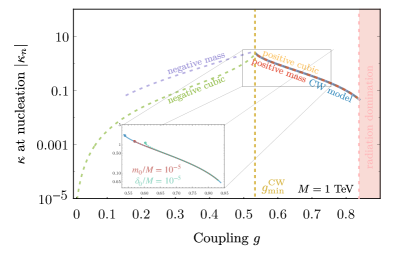
For weakly coupled theories, in the minimal setup, the dilaton potential is dominated by thermal corrections, as it is in the Coleman-Weinberg model Coleman:1973jx ; Dolan:1974gu ; Fukuda:1975di ; Kang:1974yj ; Weinberg:1992ds or the Gildener-Weinberg model Gildener:1976ih . Moreover, the dynamics of the PT can be fully captured in the high-temperature expansion. We show how cubic thermal corrections become dominant near the boundary of the supercooling window, where the expected signal is the strongest. This observation allow us to find an analytic approximation of the boundary of the supercooling window which we present in Eq. (20) and agrees astonishingly well with the full numerics as shown in Fig. 2.
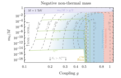
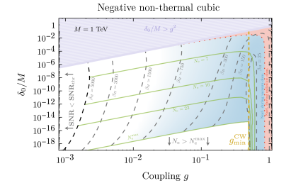
The supercooling window can be enlarged with respect to the purely radiative case by adding a small temperature-independent deformation destabilizing the origin at low enough temperatures, hence ensuring the completion of the supercooled PT.111Explicit examples of this general mechanism were introduced in specific models in Ref. vonHarling:2017yew ; Iso:2017uuu . The scaling dimension of the relevant deformation (a negative mass squared or a negative cubic at weak coupling) controls the timescale of the PT which is strongly correlated with the strength of the GW signal. We show in Eq. 33 how the negative cubic favors slow first order PTs with respect to the negative mass squared leading to a wider parameter space where a strong GW signal can be realized. Our analytical estimates match the numerical results shown in Fig. 4.
Vice-versa, relevant deformations stabilizing the origin (a positive mass squared or a positive cubic at weak coupling) obstruct the completion of the PTs and must be suppressed compared to the cut-off scale, in order to ensure that the supercooling window does not shrink substantially compared to the purely radiative case. We derive a simple analytical parametric of these deformations in Eq. (40) which we compare against the full numerical solution in Fig. 6.
For strongly coupled conformal field theories (CFTs) with a holographic description in the Randall-Sundrum Rattazzi:2000hs ; Creminelli:2001th ; Randall:2006py ; Agashe:2019lhy ; Agashe:2020lfz ; DelleRose:2019pgi setup, we derive the supercooling window by refining the original argument of Ref. Kaplan:2006yi . However, we find that the calculability of the bounce action breaks down well before the boundary of the supercooling window is attained Agashe:2019lhy ; DelleRose:2019pgi ; Agashe:2020lfz .
Our paper is organized as follows: Before turning to our results, we review in Sec. II the useful formulas necessary to describe the dynamics of PTs in the early Universe. Readers already familiar with the subject may wish to skip this summary. In Section III we define the supercooling window for weakly coupled theories in the simplest setup, where the breaking of conformal invariance is fully dominated by the interactions of the dilaton with the thermal bath, while in Section III.1 we discuss departures from this configuration. In Section IV, we define the supercooling window for strongly coupled CFTs admitting a Randall Sundrum description. We conclude in Section V. The details of our fitting procedure and the behavior of the bounce action are described in Appendix A. In Appendices C and B we provide a summary of the standard formulas used to compute the GW signal and the reach of present and future experiments.
II Phase transitions toolkit
In this section we summarize the essential conventions, notations and methodology for studying cosmological first order PTs, proceeding via the nucleation and percolation of true vacuum bubbles. We encourage expert readers to skip this section and proceed to Section III, although here and in Appendix B we provide a careful treatment of the approximations used to derive analytical results in the proceeding sections.
The nucleation rate of true vacuum bubbles is controlled by the tunneling rate between the scalar potential’s false and true vacuum due to either thermal222We use a simplified expression for the pre-factor of the thermal tunnelings’ exponent, instead of the usual approximation . This simplification does not lead to qualitative changes in the results, but does allow analytic results to be derived. or quantum fluctuations
| (1) |
Under the assumption of spherically symmetric bubbles Coleman:1977py ; Coleman:1977th and for a single scalar field controlling the tunneling rate is defined by the -dimensional O()-symmetric Euclidean action
| (2) |
where with and being the Euclidean time and position and is the wave function renormalization. To determine the initial bubble radius appearing in Eq. (1), one must solve the field profile that satisfies the so called “bounce” equation of motion
| (3) |
with boundary conditions and . Here the metastable vacuum is assumed to lie at the origin and is the location of a deeper minimum in the potential. The final step requires inserting the solution for into the action in Eq. 2 and minimizing with respect to the radius.
In what follows we make extensive use of the re-parameterization invariance of Eq. 3, and the induced re-scaling of Eq. 2. More specifically an appropriate choice of field and coordinate transformations can be used to reduce the number of free parameters controlling the scalar potential. Starting from Eq. (2), we may write the action as
| (4) |
utilizing and . We then obtain the dimensionless action and scalar potentials (denoted with a tilde)
| (5) |
As we will show the dimensionless action reduces weakly coupled renormalizable models to a single parameter system.
We now detail the micro-physics inputs required to describe the PT: i) the PT strength , ii) the duration of the PT and how it connects to the bubble size at collision iii) the time at which the PT completes. The last parameter to predict the GW spectrum is the wall velocity which depends on the interactions of the expanding vacuum bubble with the surrounding plasma. We detail the exact treatment of these dynamics for our numerical results in Appendix B.
The strength of the transition parameterizes the amount of energy available for GW production, in the form of latent heat normalized by the radiation energy density
| (6) |
where is the positive potential difference between the false and true vacuum at a given temperature and the contribution of the temperature derivative of the effective potential can be easily neglected for supercooled PTs Espinosa:2010hh . The radiation energy density is with , where encodes the usual SM radiation degrees of freedom and is model dependent.
Next we define the timescale of the PT. The nucleation rates in Eq. 1 are dominated by their exponents. Expanding these around , the transition timescale for a thermal PT can be defined as
| (7) |
where . For fast enough PT’s (i.e. ) the time of the PT can be easily related to the mean bubble size at Turner:1992tz
| (8) |
where is the probability of finding a point in the false vacuum Coleman:1977py ; Guth:1979bh ; Guth:1981uk . In Appendix B we detail the behavior , but for fast enough PTs we can approximate Eq. 8 as assuming that . Interestingly one can show that the bubble size maximizing the energy distribution satisfies which agrees with the standard formula as long as is large enough (see Appendix B for a detailed derivation).
For thermal PTs, the critical temperature is defined as the point where true and false vacuum are degenerate: . As the temperature decreases, the tunneling rate grows quickly, leading to the nucleation temperature , which marks the onset of the PT. This is defined by the time-integrated probability of a single bubble being nucleated per Hubble volume reaching one. This can be approximated as Ellis:2018mja ; Ellis:2019oqb , where is the usual Hubble rate . This is well approximated by for supercooled PTs. If the PT is fast enough, the nucleation temperature is a good approximation of . Throughout the analytic section of this work we use . In Appendix B we show that this approximation deviates at most by 20% by the percolation temperature defined as . For numerical results we use throughout as it gives a more accurate determination of .
III The supercooling window at weak coupling
At the renormalizable level, the most general potential for a single real scalar may be written as
| (9) |
where the vacuum energy can always be set to zero, and any tadpole in reabsorbed via a linear redefinition. In general, , and are complicated functions of the temperature and of any other couplings or mass scales in the theory. The re-parameterization invariance introduced in Eq. 5 allows us to rewrite the potential as a function of a single parameter. Identifying
| (10) |
yields
| (11) |
where takes values between and the scalar kinetic term is canonically normalized (). The equation defines the critical temperature where the two minima of the potential in Eq. 11 are exactly degenerate.333Strictly speaking a bounce can be defined for , where the origin becomes the global minimum and the far away vacuum the false one. For larger than the potential in Eq. 11 has only one global minimum at the origin.
The bounce solution can be deduced once and for all by numerically computing the bounce for different values of and then performing a one-parameter fit (see Ref. Adams:1993zs ; Sarid:1998sn for similar results). For weakly coupled theories the tunneling rate is always dominated by thermal fluctuations (see Appendix A) and we can take neglecting 1-loop correction to the wave function. Using this approach the symmetric bounce action can be written as
| (12) |
where is given explicitly in Appendix A and it is defined such that and the two fitting functions match at where the bounce action admits a known analytical limit Brezin:1978 . For the functional dependence for is fixed to reproduce the thin-wall approximation at zeroth order in the thin-wall expansion Coleman:1977py . The subleading terms computed in Ref. Ivanov:2022osf do not impact significantly our results. For the solution is chosen such that for we recover the solution of Ref. Brezin:1992sq .
III.1 Radiative breaking of conformal symmetry
Taking the theory to be classically scale invariant, and assuming the thermal corrections to be dominated by a single coupling , we obtain simple expressions for the parameters of the scalar field potential in the high- expansion:
| (13) |
where is the number of the bosonic degrees of freedom in the thermal bath.444 Fermionic and bosonic degrees of freedom both contribute to the thermal potential. We assume to get a positive quartic from radiative corrections.
In these scenarios, the classically flat direction is lifted by radiative corrections, which generate a stable vacuum at where conformal symmetry is radiatively broken. At the true minimum, the heavy states obtain a mass of order , while the scalar flat direction mass is loop suppressed . At zero temperature, the energy difference between the stable minimum and the origin is therefore of order .
Concrete realizations of this scaling are the Coleman-Weinberg model (CW model) Coleman:1973jx ; Dolan:1974gu ; Fukuda:1975di ; Kang:1974yj ; Weinberg:1992ds , consisting of a complex scalar charged under a gauge symmetry with coupling strength and the Gildener-Weinberg setup (GW model) Gildener:1976ih which consists of real scalars coupled through quartic interactions with strength . For simplicity, we present our results in terms of the CW model where and define where and is the renormalization scale in the scheme. The potential energy difference at zero temperature is proportional to as
| (14) |
Our results easily generalize to the GW model by replacing and to account for numerical factors coming from the different finite pieces in the 1-loop potential between vector and scalar normalization.
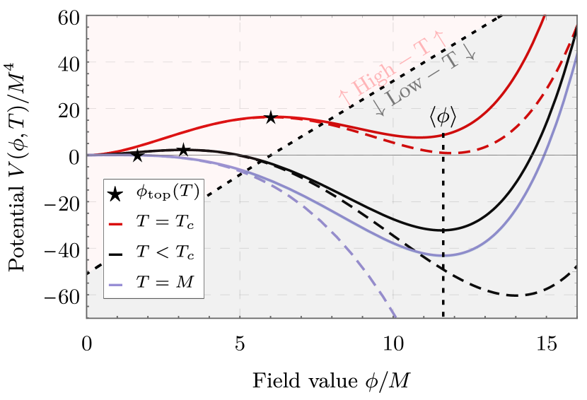
We now proceed to describing the thermal history of the CW model. At early times, the origin is the true vacuum of the theory. As the Universe cool down, the dilaton potential undergoes a PT whose dynamics can be fully captured within the high- expansion of Eq. 13 as shown in Fig. 1. This can be verified by tracking the position of the top of the barrier between the two vacua , whose existence ensures that the PT is of the first order. We find that , where is the value of at the critical temperature , with estimated in the high-T expansion. This ratio scales as easily satisfying the high- condition at the temperatures which are relevant for the PT dynamics.
Since the onset of nucleation is governed by the nucleation condition becomes
| (15) |
In the parametrization of Eq. 11 the bounce action reads
| (16) |
where we used the relations and . Equipped with Eq. 16, we can now study the parametric dependence of the first order PT on the gauge coupling .
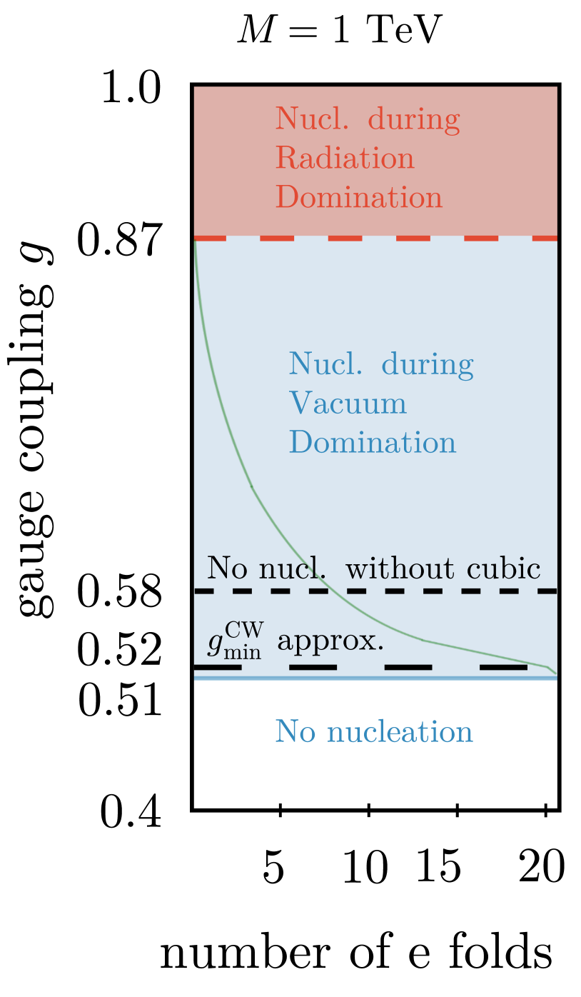
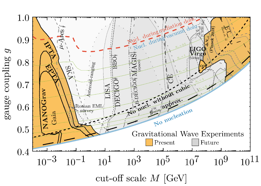
We are particularly interested in understanding the boundaries of the supercooling region – defined as the regime where a first order PT completes with (i.e. after a period of inflation). Our results are summarized in Fig. 2 where we observe the following: i) The lower bound on separates the region where the PT completes from the region where inflation does not end. ii) The upper bound on separates the supercooling region from the region where the first order PT completes during radiation domination.
Interestingly, from the right panel of Fig. 2 we see that the totality of the supercooling window can be probed at future GW detection experiments as long as the scale of the PT lies below (with the usual optimism in the expected reach of proposed future experiments as detailed in Appendix B). We checked that this conclusion is unaffected by possibly larger astrophysical background in the LIGO frequency band Zhou:2022otw ; Zhou:2022nmt , essentially because of the enormous GW signal generated by the supercooled PTs.
As we see from Fig. 2, the lower bound on the gauge coupling is of crucial phenomenological relevance since it distinguishes a strong first order PT from a regime in which the period inflation is eternal and its fate depends on the behavior of quantum fluctuations Kearney:2015vba ; Joti:2017fwe ; Lewicki:2021xku . The upper bound of the supercooling window is instead only indicating where stops being larger than . This does not have an immediate phenomenological impact since, depending on the experiment, first order PTs with can also lead to a detectable GW signal.
The number of e-foldings of inflation before the PT completes is defined as
| (17) |
with being the temperature where the energy density in radiation and vacuum energy is equal. In Fig. 2 and all subsequent figures we show as light green contours. The number of e-folds is bounded from above by requiring i) quantum fluctuations of the dilaton field to be negligible, ii) the CMB power spectrum to match the Planck observations Planck:2018jri . These two constraints require to be less than and respectively and ended up being unimportant in the phenomenologically interesting region of the CW model.
In the remainder of this section we derive analytic expressions for the lower and upper boundaries of the supercooling window in the CW model.
The lower bound on supercooling
can be defined by studying the nucleation condition during vacuum domination (VD), which reads
| (18) |
where we defined . We have taken the expression for the bounce action, defined in Eq. 16, as is expected to hold in this regime. An approximate formula for the boundary of nucleation in the large supercooling limit can be found by expanding the above expression for (i.e. )
| (19) |
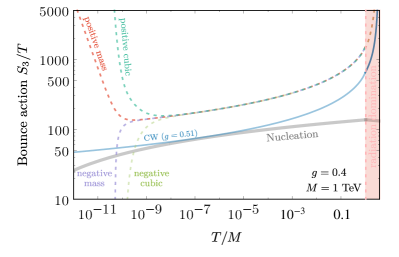
where the constant term on the left-hand side is the leading-order contribution to the bounce due to the cubic scalar self-interaction introduced in Eq. 11. Naively, one would like to approximate the nucleation temperature by ignoring the constant term and getting a simple analytical solution , which is often quoted in the literature. However, this approximation is only justified for which in practice is never realized in the relevant parameter space. The actual behavior of is shown in Fig. 3 right where we can see that at the boundary of the supercooling window. Therefore, the thermal cubic should be included in order to reliably describe the nucleation in the deep supercooling regime. We find that the solution of Eq. (19) approximate up to corrections which correspond to having neglected the higher orders in the expansion. Luckily these corrections have a negligible impact on the determination of lower bound on the supercooling window.
Studying the zeros of the discriminant of Eq. (19) we can find the boundary values of that give an interception point between the bounce action and the nucleation curve. The discriminant is a cubic equation in with coefficients depending on so that the boundary of the supercooling window corresponds to a single real solution if the discriminant is negative or the smallest of the three real solutions if the discriminant is positive.555For completeness we give the full equation describing the zeros of the discriminant here in terms of : with , and . Series expanding the result to yields
| (20) |
This corresponds to the minimal nucleation temperature at which the PT completes avoiding eternal inflation. The leading term in Eq. 20 is , which corresponds to the lowest possible coupling neglecting the thermal cubic contribution. The new correction proportional to is controlled by the thermal cubic whose role is to reduce the value of , enlarging the supercooling window. Fig. 2 shows that our analytic approximation (dashed black line) reproduces very well the boundary of the supercooling window obtained by a brute force numerical scan which is plotted in blue (see Ref. Azatov:2019png for a similar numerical analysis of the CW model).
The value of is also modified by next-to-leading order corrections to the thermal potential. The inclusion of daisy diagrams Dolan:1973qd ; Carrington:1991hz ; Delaunay:2007wb ; Curtin:2016urg , i.e. a resummation of the leading-order hard thermal loops, serve to reduce the thermal barrier and subsequently extend the parameter space where nucleation is viable. In the language of Eq. 13, we can write the shift in the mass and cubic induced by these corrections as
| (21) | ||||
| (22) |
Note that these closed form expressions require series expanding in small , which is a good assumption around the thermal barrier, as well as a field redefinition to remove the term that arises linear in . Here we see that the inclusion of Daisy diagrams decrease while simultaneously increasing the size of the negative cubic throughout the supercooling regime. The effects of the Daisy diagrams accounts for the difference between the analytic approximation in Eq. 20 and the full numerical result in Fig. 2.
The upper bound on supercooling
can be defined imposing , where is the temperature below which the Hubble rate shifts from radiation to vacuum dominated and reads
| (24) |
where we used the energy difference between the false and true vacuum at zero temperature in the CW model, see Eq. 14. The nucleation condition defining can be written as
| (25) |
where for , the quartic implies as follows from Eq. 11 allowing for a simple parameterization of . The equation above is an algebraic equation which defines and can be solved in general. This is shown as a dashed red curve in the right-hand panel of Fig. 2.
III.2 Additional sources of explicit breaking
We now wish to study the consequences of incorporating additional scales breaking explicitly the conformal symmetry in the zero temperature potential. In the high temperature expansion, these deformations can be parameterized as shifts of the temperature dependent terms in Eq. 13. In what follows we study the set of possible deformations, examining how their presence changes the behavior of and ultimately the possibility of realizing supercooled PTs. A schematic view of how these deformations affect is presented in Fig. 3 left. In Sec. III.2.1 we describe deformations destabilizing the origin with either a negative squared mass or a cubic.666Note that here we use the terminology positive or negative with respect to its sign in the scalar potential. These will make decreasing at low temperature as shown by the violet and green lines in Fig. 3, hence enlarging the supercooling window compared to the CW case as shown in Fig. 4. In Sec. III.2.2 we describe deformations stabilizing the fake vacuum at origin with either a positive squared mass or a positive cubic. These will make increasing at low temperature as shown by the red and orange lines in Fig. 3, hence shrinking the supercooling window compared to the CW case as shown in Fig. 6.
III.2.1 Enlarging the supercooling window
Here, we would like to explore how the boundary of the supercooling window is extended as explicit breaking contributions destabilizing the origin are added to Eq. 13. This prospect can be studied by introducing non-thermal relevant deformations, which act to eliminate the thermally induced barrier at some finite temperature , implying that the PT necessarily completes, even outside of the classically invariant supercooling window. The obvious candidates are a negative mass or a negative cubic term , whose bounce actions are shown in the left panel of Fig. 3. In this figure, the bounce follows the conformal case until it reaches temperatures comparable to the scale of the relevant deformations, where it quickly drops to zero corresponding to lowering the thermal barrier.
If nucleation only occurs just before (or after) the thermal barrier disappears the PT is effectively second order and no strong GW signal is expected. The relevant question to quantify here is then how large is the parameter space where the PT completes with a large enough GW signal. As we will see this depends very much on the scaling of , which is controlled by the slope of the bounce action drop and very sensitive to the scaling dimension of the temperature-independent deformation.
The effects of introducing small temperature-independent deformations can easily encoded in the high- expansion as
| (26) | ||||
| (27) |
Importantly, the negative non-thermal cubic also affects the thermal mass at one loop, as
| (28) |
where we expanded the loop contribution at leading order for small . The mass shift arises from the tadpole for , induced at one-loop by the presence of the cubic. Performing a field redefinition to remove this term gives rise to the shift in Eq. 28.
As can be seen from Eqs. 28 and 26, for both deformations there is a temperature such that the effective thermal mass vanishes: . In the region of interest the nucleation temperature should be very close to . Approaching the parameter defined in Eq. 11 tends to zero as explicitly shown in the right panel of Fig. 3. These two features characterize the dynamics of PTs that complete for , where the nucleation is triggered mostly by the temperature-independent deformations.
To describe this region we can then work under two simplifying assumptions: ) we take to be a small parameter keeping only the leading order term in the expansion, ) we expand the bounce action for . In this limit the bounce action can be written in general as
| (29) |
Setting we can use Eq. 29 to get a simple expression for the nucleation temperature around the limit of a vanishing barrier:
| (30) |
Lastly, we can estimate the timescale of the PT by expressing in the same limit
| (31) |
where we already substituted the value of obtained in Eq. (30).
The above formulas can be used to get simple parameterics for the two deformations at hand. Finding the zeroes of Eqs. 26 and 28 we get at first order in to be
| (32) |
from which one can easily derive the behavior of and in the two cases. Putting all these together we get the asymptotic behavior of for for the two deformations:
| (33) |
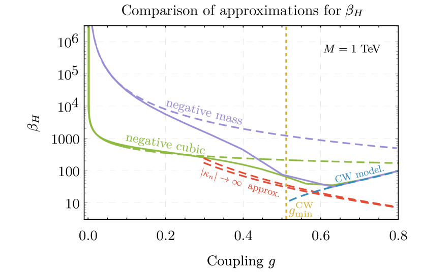
The different scaling of with the gauge coupling can be simply understood from Eq. (31) by remembering that for the for the mass deformation: , and ; while for the cubic deformation: , and . The asymptotic behavior of Eq. (33) agrees extremely well with the full numerical result for as shown in Fig. 5. In the same figure we show the departure from CW behavior. This behavior is universal in both cases and can be easily derived as (dashed red line).
As a result, our parametric can easily explain why the cubic deformation enlarges the supercooling parameter space so much more than the mass one as shown in Fig. 4. The scaling dimension of the deformation controls the dependence of on which ultimately sets the strength of GW signal.
The left boundary for small in Fig. 4 is determined purely by which controls both the strength and the peak frequency of the PT in the limit where (see Appendix C for details). In particular if we focus on the sound wave contribution, that typically dominates the GW production in our setup, the peak frequency scales as while the signal strength scales as . The precise boundary of the parameter space will depend on the details of the signal and the experimental reach and we do not find it particularly enlightening to quantify. Our shading in Fig. 4 indicates that are the maximal allowed to obtain a detectable GW signal at any frequency, although for particular frequency windows the amazing expected reach of future GW interferometers could probe even larger values of .
The fact that the size of the deformation cannot be too small compared to the cut-off can be easily understood from the fact that the smaller the deformation, the longer the bounce will track the CW solution before nucleation, resulting in a larger number of e-folds of inflation as defined in Eq. 17. The upper bound on the number of e-folds of inflation gives a lower bound on and hence a lower bound on the size of the deformation which is shown in Fig. 4.
Before concluding this section, we briefly comment on explicit models where the cubic deformation dominates over the mass and the quartic. One example is the linear coupling of the CW dilaton to an operator which dynamically develops a vacuum expectation value. The dilaton potential at zero temperature can be schematically written as
| (34) |
where in the CW model and we added the VEV of an operator of dimension with . Shifting the tadpole term by using the field redefinition induces a mass and negative cubic terms for scaling as . In the limit the induced mass becomes sub-dominant compared to the cubic, which is the leading deformation from classical scale invariance. This model can then be mapped to our parametrization above by identifying . Explicit examples were discussed in Refs. vonHarling:2017yew ; Iso:2017uuu .
In realistic scenarios both a positive mass squared and a cubic deformation will be generated at tree level, so we briefly discuss how our result is modified when both and are present. As shown in Fig. 3 if a large positive non-thermal mass squared dominates the dynamics, it will make the bounce growing to infinity at low temperatures before meeting the nucleation condition. The existence of a solution to requires then an upper bound on , which however does not seem to require any additional fine-tuning to be fulfilled.
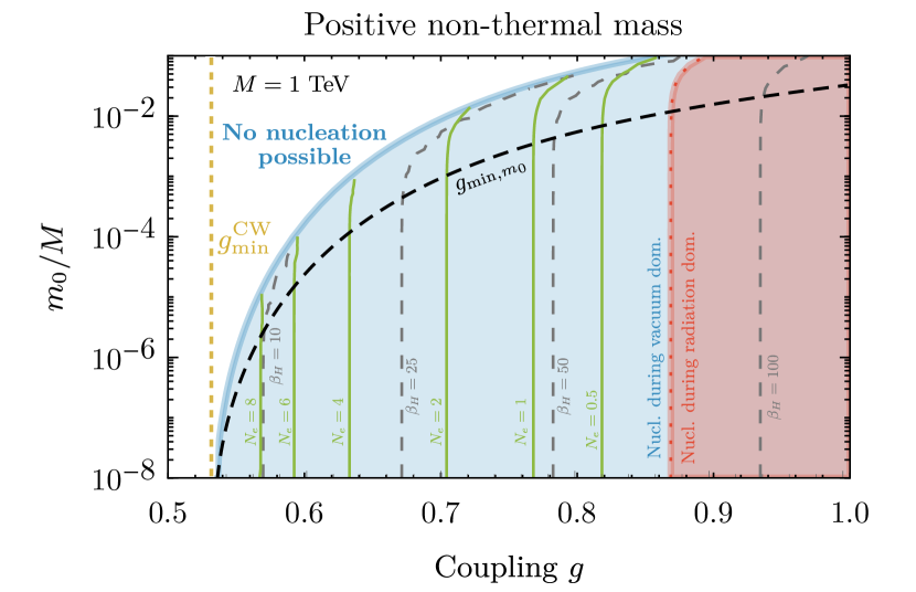
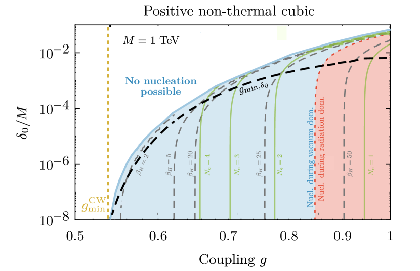
III.2.2 Shrinking the supercooling window
In this section we study how the boundary of the supercooling window shrinks once deformations stabilizing the origin are added to Eq. 13. In contrast to the CW case, the action in these cases does not continue to decrease indefinitely. From both the red and orange curves in Fig. 3 we observe that the action reaches a minimum at a temperature comparable to the size of the explicit breaking. Hence, it is expected that for sufficiently large values of the explicit breaking parameter nucleation will be prevented.
We will examine the case of a positive mass-squared and that of a positive cubic term which can be easily captured in the high- expansion by shifting the thermal mass and cubic in Eq. 13 respectively:
| (35) | |||
| (36) |
In both cases, when the deformations are small, the supercooling boundary can be determined by expanding the action to leading order in , keeping the first non-trivial correction due to or . The right panel of Fig. 3 confirms that this approximation is justified. In the large limit the bounce action admits the following simple form
| (37) |
where can be easily found for the two deformations of interest:
| (38) |
At zeroth order in the expansion of we can express the new supercooling window boundary, as
| (39) |
where is the CW result of Eq. 20 and encodes the effects of the explicit breaking. Solving the nucleation condition we get
| (40) |
The shrinking of the supercooling window can then be understood by studying the properties of given in Eq. 40. Namely, is minimized for (corresponding to the zeroth order conformal result) and otherwise it is an increasing function of . Since for the deformations in question we always find that it is clear that increases with , reducing the viable parameter space for supercooling.
The only remaining step to obtain the supercooling boundary is determining which amounts to find the minimum of Eq. 37. For the two deformations under consideration we find
| (41) |
with for the mass case and in the cubic case. Plugging the expressions from Eq. 41 into Eq. (40) we explicitly see that as get larger, the value of increases until the supercooling window closes completely. Since the for the cubic deformation increases parameterically faster as a function of than in the mass case, the corresponding supercooling parameter space shrinks faster than in the mass case as shown in Fig. 6.
The full behavior of the deformation dependent shift for both deformations is shown in Fig. 6, where we also plot the behavior of the nucleation temperature and of . Our crude approximation in Eq. (40) (shown as the black dashed line in Fig. 6) captures only the qualitative behavior of the boundary but fails completely as soon as the deformation become sufficiently large.
From Fig. 6 we clearly see that the deformation term should be at least loop suppressed in order for the supercooling window to not shrink completely.
IV The supercooling window at strong coupling
In this section, we derive the supercooling window for a class of strongly coupled theories which have a known holographic dual. We focus on large CFT with spontaneously broken conformal symmetry where the dilaton potential and the holographic principle Maldacena:1997re ; Randall:1999ee can be used to trace the PT between broken and unbroken conformal symmetry as first shown in Ref. Creminelli:2001th .
If conformal invariance is mainly spontaneously broken, the confined phase can be well described by the effective dilaton potential, radiatively generated by the coupling of the dilaton to a marginally irrelevant operator of dimension with coupling strength . The zero temperature dilaton potential describing the confined phase can be written as
| (42) |
where is the dilaton VEV which is defined in terms of the cut-off as . Here and are the values of the dilaton quartic and the coupling strength at the UV scale . Moreover, we have expanded the running dilaton quartic at the leading order in small , defining .
The above construction can be viewed as the holographic dual of a 5-dimensional theory of gravity in anti-de Sitter space with IR and UV branes Randall:1999ee stabilized by the Goldberger-Wise mechanism Goldberger:1999uk ; Goldberger:1999un . The dilaton is interpreted as the radion, describing the position of the IR brane. A non-flat radion potential is therefore associated with the breaking of conformal symmetry. The dilaton potential in Eq. 42 can be shown to match the radion potential, for small .
We take as the bare dilaton quartic and parametrizes the small positive anomalous dimension. The normalization of the dilaton potential can be obtained via the AdS/CFT correspondence or directly by considering the contribution of the irrelevant operator to the trace anomaly Rattazzi:2000hs ; Arkani-Hamed:2000ijo . The smallness of , determines the hierarchy of scales between the dilaton and the other CFT states so that the vacuum structure can be studied in terms of the dilaton potential alone. This is analogous to the loop suppression of the dilaton mass in the CW model of Sec. III.1. We also assume the number of degrees of freedom contributing thermally to the dilaton potential after confinement to be small which requires .
At high temperatures, the system is in its deconfined phase, consisting of a strongly coupled large CFT. The contribution of the thermal CFT plasma to the free energy is as supported by holographic results Witten:1998zw . The details of the full potential in this phase depends on the strongly coupled dynamics and are incalculable. This introduces a certain arbitrariness in matching the dilaton potential in the confined phase with the value of the free energy in the deconfined phase (see Refs. Agashe:2019lhy ; DelleRose:2019pgi ; Agashe:2020lfz for an extensive discussion). The simplest option is to take
| (43) |
where the two sides of the potential are then glued together at the origin of field space and the dilaton potential in the deconfined/confined phases is denoted by negative/positive field values for , respectively. In what follows, we will show the region of parameter space which is insensitive to the choice of deconfined potential.
The potential energy difference between the false vacuum at the origin and the dilaton VEV at zero temperature is simply
| (44) |
where is the effective confinement scale, defined similarly to Kaplan:2006yi . The free energies of both phases equilibrate at , so that a (de)confining PT which completes at must always be supercooled, as . This is in sharp contrast with the weak coupling case where the same model could describe a PT both in vacuum and radiation domination.
The full potential describing the PT dynamics is then given by the sum of the confined and the deconfined dilaton potential and can be written as
| (45) |
where we used the reparametrization invariance defined in Eq. (5) with
| (46) |
to get a lagrangian that up to an overall rescaling by , depends only on a single parameter
| (47) |
Here, ranges between , where its critical value is , at which the two phases have the same vacuum energy.
The dimensional bounce action is given by
| (48) |
where is a fitting function regularized over the TW solution, admitted near the critical value . Unlike in the weakly coupled case, the thermally driven bounce does not always dominate, hence the tunneling rate is dictated by the . Due to their different scaling with , it is expected that for sufficiently low and the quantum contribution may dominate, i.e. . Explicit forms for the actions, as well as a comparison between the two, are given in Appendix A. In Section A.2 we find that for the majority of the relevant parameter space, quantum tunneling dominates and ultimately controls the boundary of nucleation.
The supercooling boundary can now be found by solving the induced nucleation condition Eq. 15 in the limit (i.e. ). admits a simple solution for the nucleation temperature, given explicitly in Eq. 68, with the lowest possible temperature obtained at
| (49) |
Requiring sets a lower bound on the explicit breaking of conformal symmetry as
| (50) |
In deriving Eq. 49, we completely ignored the contribution to the action due to the motion along the deconfined region of the potential, i.e. . We can estimate the contribution of this motion to the bounce in the TW approximation Agashe:2019lhy ; DelleRose:2019pgi neglecting friction, as
| (51) |
where is the critical bubble size, resulting in
| (52) |
Note that the surface tension in Eq. 51 is integrated between and , implicitly taking the dilaton potential on the CFT side to be minimized at . While this assumption is well motivated in the holographic picture by the existence of the AdS black hole solution Creminelli:2001th , relaxing it can drastically change the values of the bounce actions in Eq. 52, which scale linearly with the CFT vacuum position as .
The truly calculable region of parameter space is then defined by requiring , which sets an upper boundary on the explicit breaking of conformal symmetry
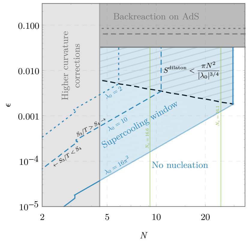
| (53) |
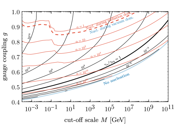
In Fig. 7 we show the supercooling window for a strongly coupled CFT as a function of and , fixing the confinement scale and varying the bare quartic . The only calculable boundary of the window is the one for smaller which is the analogous of the small boundary in the weakly coupled case. As already noticed in Ref. Kaplan:2006yi requiring a non-empty Universe imposes a strong upper bound on which can be large enough to justify the large expansion only for very large values of the dilaton quartic .
V Conclusions
Supercooled PTs offer one of the best possibilities to produce sizeable GW stochastic backgrounds in the early Universe. This motivated us to understand their dynamics systematically, characterizing the available parameter space with the goal of understanding how generic a supercooled PT can be. This is critical as it is well known that supercooled PTs live at the boundary of eternal inflation Guth:2007ng ; Kaplan:2006yi ; Arkani-Hamed:2007ryv ; Dubovsky:2011uy . In practice this implies for minimal models that the coupling constant controlling the close-to-marginal operator breaking conformal symmetry has to be judiciously chosen to allow the PT to complete. As a starting point of our analysis we quantify precisely the allowed range for this coupling which we call the supercooling window for weakly coupled and strongly coupled theories.
The boundary of the supercooling window at weak coupling where conformal symmetry is radiatively broken is well described by a simple formula we derived in Eq. 20 up to the daisy resummation of the thermal loops (see Fig. 2). Our simple formula highlights the importance of the thermally generated cubic which was neglected in previous analytical approximations. This contribution dominates the dynamics close to the boundary of the supercooling window because it reduces the thermal barrier hence favoring bubble nucleation. At the same time, the small range of couplings where supercooling can be realized suggests looking beyond the minimal model.
Depending on their relative sign with respect to the thermal contributions, small zero-temperature deformations of the potential can either increase or decrease the size of the thermal barrier between the false vacuum and the true vacuum. While in the former case the supercooling window obviously shrinks, it is interesting to ask what happens in the latter case where at some sufficiently low temperature the barrier completely disappears and the PT behaves as a second order or cross-over transition.
We explicitly study the cases of mass and cubic deformation destabilizing the origin, deriving analytically the parametric scaling of the time scale of the PT (often called in the literature). We show that in both cases the supercooling window is enlarged with respect to the minimal case. Compared to the mass case, the cubic deformation gives a wider region where a strong first order PT completes before the barrier disappears. This can be understood analytically from Eq. (33) comparing how fast the the barrier disappears with respect to the time scale of nucleation. Adding a cubic deformation makes the supercooling window wide enough at the price of realizing a large hierarchy between the dynamics generating the cubic deformation and the one responsible for the spontaneous breaking of conformal symmetry. Examples of concrete setups were given in Ref. vonHarling:2017yew ; Iso:2017uuu .
For completeness we define the supercooling window in strongly coupled gauge theories with a holographic dual. Analogously to previous studies Gubser:1999vj ; Kaplan:2006yi we find that a successful nucleation generically challenges the large expansion and the small-backreaction limit. Our analysis reinforces the need for constructing fully calculable strongly coupled setups at large where supercooled PTs can occur. Non minimal models addressing this issue were put forward in Ref. Randall:2006py ; Nardini:2007me ; Konstandin:2011dr ; Konstandin:2010cd ; Dillon:2017ctw ; vonHarling:2017yew ; Bruggisser:2018mus ; Bruggisser:2018mrt ; Megias:2018sxv ; Bunk:2017fic ; Baratella:2018pxi ; Agashe:2019lhy ; Fujikura:2019oyi ; Azatov:2020nbe ; Megias:2020vek ; Agashe:2020lfz and more recently in Ref. Agrawal:2021alq . We hope to return to these issues in the future.
Acknowledgments
We thank Nathaniel Craig and Alberto Mariotti for collaboration at an early stage of this project, as well as Pedro Schwaller, Andrea Tesi and Lorenzo Ubaldi for many useful comments and discussions. NL would like to thank the Milner Foundation for the award of a Milner Fellowship. We thank Alberto Mariotti and Andrea Tesi for feedback on the draft.
References
- (1) LIGO Scientific, Virgo Collaboration, B. P. Abbott et al., Observation of Gravitational Waves from a Binary Black Hole Merger, Phys. Rev. Lett. 116 (2016), no. 6 061102, [1602.03837].
- (2) LISA Cosmology Working Group Collaboration, P. Auclair et al., Cosmology with the Laser Interferometer Space Antenna, 2204.05434.
- (3) G. Bertone et al., Gravitational wave probes of dark matter: challenges and opportunities, SciPost Phys. Core 3 (2020) 007, [1907.10610].
- (4) E. Witten, Cosmic Separation of Phases, Phys. Rev. D 30 (1984) 272–285.
- (5) C. J. Hogan, Gravitational radiation from cosmological phase transitions, Mon. Not. Roy. Astron. Soc. 218 (1986) 629–636.
- (6) M. Kamionkowski, A. Kosowsky, and M. S. Turner, Gravitational radiation from first order phase transitions, Phys. Rev. D 49 (1994) 2837–2851, [astro-ph/9310044].
- (7) C. Caprini and D. G. Figueroa, Cosmological Backgrounds of Gravitational Waves, Class. Quant. Grav. 35 (2018), no. 16 163001, [1801.04268].
- (8) S. R. Coleman and E. J. Weinberg, Radiative Corrections as the Origin of Spontaneous Symmetry Breaking, Phys. Rev. D 7 (1973) 1888–1910.
- (9) E. Gildener and S. Weinberg, Symmetry Breaking and Scalar Bosons, Phys. Rev. D 13 (1976) 3333.
- (10) E. Witten, Cosmological Consequences of a Light Higgs Boson, Nucl. Phys. B 177 (1981) 477–488.
- (11) T. Hambye and A. Strumia, Dynamical generation of the weak and Dark Matter scale, Phys. Rev. D 88 (2013) 055022, [1306.2329].
- (12) S. Iso, P. D. Serpico, and K. Shimada, QCD-Electroweak First-Order Phase Transition in a Supercooled Universe, Phys. Rev. Lett. 119 (2017), no. 14 141301, [1704.04955].
- (13) A. Azatov, D. Barducci, and F. Sgarlata, Gravitational traces of broken gauge symmetries, JCAP 07 (2020) 027, [1910.01124].
- (14) L. Randall and G. Servant, Gravitational waves from warped spacetime, JHEP 05 (2007) 054, [hep-ph/0607158].
- (15) G. Nardini, M. Quiros, and A. Wulzer, A Confining Strong First-Order Electroweak Phase Transition, JHEP 09 (2007) 077, [0706.3388].
- (16) T. Konstandin and G. Servant, Cosmological Consequences of Nearly Conformal Dynamics at the TeV scale, JCAP 12 (2011) 009, [1104.4791].
- (17) F. C. Adams, General solutions for tunneling of scalar fields with quartic potentials, Phys. Rev. D 48 (1993) 2800–2805, [hep-ph/9302321].
- (18) U. Sarid, Tools for tunneling, Phys. Rev. D 58 (1998) 085017, [hep-ph/9804308].
- (19) V. Guada, M. Nemevšek, and M. Pintar, FindBounce: Package for multi-field bounce actions, Comput. Phys. Commun. 256 (2020) 107480, [2002.00881].
- (20) C. L. Wainwright, Cosmotransitions: Computing Cosmological Phase Transition Temperatures and Bubble Profiles with Multiple Fields, Comput. Phys. Commun. 183 (2012) 2006–2013, [1109.4189].
- (21) L. Dolan and R. Jackiw, Gauge Invariant Signal for Gauge Symmetry Breaking, Phys. Rev. D 9 (1974) 2904.
- (22) R. Fukuda and T. Kugo, Gauge Invariance in the Effective Action and Potential, Phys. Rev. D 13 (1976) 3469.
- (23) J. S. Kang, Gauge Invariance of the Scalar-Vector Mass Ratio in the Coleman-Weinberg Model, Phys. Rev. D 10 (1974) 3455.
- (24) E. J. Weinberg, Vacuum Decay in Theories with Symmetry Breaking by Radiative Corrections, Phys. Rev. D 47 (1993) 4614–4627, [hep-ph/9211314].
- (25) B. von Harling and G. Servant, QCD-Induced Electroweak Phase Transition, JHEP 01 (2018) 159, [1711.11554].
- (26) R. Rattazzi and A. Zaffaroni, Comments on the holographic picture of the Randall-Sundrum model, JHEP 04 (2001) 021, [hep-th/0012248].
- (27) P. Creminelli, A. Nicolis, and R. Rattazzi, Holography and the Electroweak Phase Transition, JHEP 03 (2002) 051, [hep-th/0107141].
- (28) K. Agashe, P. Du, M. Ekhterachian, S. Kumar, and R. Sundrum, Cosmological Phase Transition of Spontaneous Confinement, JHEP 05 (2020) 086, [1910.06238].
- (29) K. Agashe, P. Du, M. Ekhterachian, S. Kumar, and R. Sundrum, Phase Transitions from the Fifth Dimension, JHEP 02 (2021) 051, [2010.04083].
- (30) L. Delle Rose, G. Panico, M. Redi, and A. Tesi, Gravitational Waves from Supercool Axions, JHEP 04 (2020) 025, [1912.06139].
- (31) J. Kaplan, P. C. Schuster, and N. Toro, Avoiding an Empty Universe in RS I Models and Large-N Gauge Theories, hep-ph/0609012.
- (32) S. R. Coleman, The Fate of the False Vacuum. 1. Semiclassical Theory, Phys. Rev. D 15 (1977) 2929–2936. [Erratum: Phys.Rev.D 16, 1248 (1977)].
- (33) S. R. Coleman, V. Glaser, and A. Martin, Action Minima Among Solutions to a Class of Euclidean Scalar Field Equations, Commun. Math. Phys. 58 (1978) 211–221.
- (34) J. R. Espinosa, T. Konstandin, J. M. No, and G. Servant, Energy Budget of Cosmological First-order Phase Transitions, JCAP 06 (2010) 028, [1004.4187].
- (35) M. S. Turner, E. J. Weinberg, and L. M. Widrow, Bubble nucleation in first order inflation and other cosmological phase transitions, Phys. Rev. D 46 (1992) 2384–2403.
- (36) A. H. Guth and S. H. H. Tye, Phase Transitions and Magnetic Monopole Production in the Very Early Universe, Phys. Rev. Lett. 44 (1980) 631. [Erratum: Phys.Rev.Lett. 44, 963 (1980)].
- (37) A. H. Guth and E. J. Weinberg, Cosmological Consequences of a First Order Phase Transition in the SU(5) Grand Unified Model, Phys. Rev. D 23 (1981) 876.
- (38) J. Ellis, M. Lewicki, and J. M. No, On the Maximal Strength of a First-Order Electroweak Phase Transition and its Gravitational Wave Signal, JCAP 04 (2019) 003, [1809.08242].
- (39) J. Ellis, M. Lewicki, J. M. No, and V. Vaskonen, Gravitational wave energy budget in strongly supercooled phase transitions, JCAP 06 (2019) 024, [1903.09642].
- (40) E. Brézin and G. Parisi, Critical exponents and large-order behavior of perturbation theory, Journal of Statistical Physics 19 (1978), no. 3 269–292.
- (41) A. Ivanov, M. Matteini, M. Nemevšek, and L. Ubaldi, Analytic thin wall false vacuum decay rate, JHEP 03 (2022) 209, [2202.04498].
- (42) E. Brezin and G. Parisi, Critical exponents and large order behavior of perturbation theory, .
- (43) B. Zhou, L. Reali, E. Berti, M. Çalışkan, C. Creque-Sarbinowski, M. Kamionkowski, and B. S. Sathyaprakash, Compact Binary Foreground Subtraction in Next-Generation Ground-Based Observatories, 2209.01221.
- (44) B. Zhou, L. Reali, E. Berti, M. Çalışkan, C. Creque-Sarbinowski, M. Kamionkowski, and B. S. Sathyaprakash, Subtracting Compact Binary Foregrounds to Search for Subdominant Gravitational-Wave Backgrounds in Next-Generation Ground-Based Observatories, 2209.01310.
- (45) J. Kearney, H. Yoo, and K. M. Zurek, Is a Higgs Vacuum Instability Fatal for High-Scale Inflation?, Phys. Rev. D 91 (2015), no. 12 123537, [1503.05193].
- (46) A. Joti, A. Katsis, D. Loupas, A. Salvio, A. Strumia, N. Tetradis, and A. Urbano, (Higgs) vacuum decay during inflation, JHEP 07 (2017) 058, [1706.00792].
- (47) M. Lewicki, O. Pujolàs, and V. Vaskonen, Escape from supercooling with or without bubbles: gravitational wave signatures, Eur. Phys. J. C 81 (2021), no. 9 857, [2106.09706].
- (48) Planck Collaboration, Y. Akrami et al., Planck 2018 results. X. Constraints on inflation, Astron. Astrophys. 641 (2020) A10, [1807.06211].
- (49) L. Dolan and R. Jackiw, Symmetry Behavior at Finite Temperature, Phys. Rev. D 9 (1974) 3320–3341.
- (50) M. E. Carrington, The Effective potential at finite temperature in the Standard Model, Phys. Rev. D 45 (1992) 2933–2944.
- (51) C. Delaunay, C. Grojean, and J. D. Wells, Dynamics of Non-renormalizable Electroweak Symmetry Breaking, JHEP 04 (2008) 029, [0711.2511].
- (52) D. Curtin, P. Meade, and H. Ramani, Thermal Resummation and Phase Transitions, Eur. Phys. J. C78 (2018), no. 9 787, [1612.00466].
- (53) J. M. Maldacena, The Large N limit of superconformal field theories and supergravity, Adv. Theor. Math. Phys. 2 (1998) 231–252, [hep-th/9711200].
- (54) L. Randall and R. Sundrum, A Large mass hierarchy from a small extra dimension, Phys. Rev. Lett. 83 (1999) 3370–3373, [hep-ph/9905221].
- (55) W. D. Goldberger and M. B. Wise, Modulus stabilization with bulk fields, Phys. Rev. Lett. 83 (1999) 4922–4925, [hep-ph/9907447].
- (56) W. D. Goldberger and M. B. Wise, Phenomenology of a stabilized modulus, Phys. Lett. B 475 (2000) 275–279, [hep-ph/9911457].
- (57) N. Arkani-Hamed, M. Porrati, and L. Randall, Holography and phenomenology, JHEP 08 (2001) 017, [hep-th/0012148].
- (58) E. Witten, Anti-de Sitter space, thermal phase transition, and confinement in gauge theories, Adv. Theor. Math. Phys. 2 (1998) 505–532, [hep-th/9803131].
- (59) A. H. Guth, Eternal inflation and its implications, J. Phys. A 40 (2007) 6811–6826, [hep-th/0702178].
- (60) N. Arkani-Hamed, S. Dubovsky, A. Nicolis, E. Trincherini, and G. Villadoro, A Measure of de Sitter entropy and eternal inflation, JHEP 05 (2007) 055, [0704.1814].
- (61) S. Dubovsky, L. Senatore, and G. Villadoro, Universality of the Volume Bound in Slow-Roll Eternal Inflation, JHEP 05 (2012) 035, [1111.1725].
- (62) S. S. Gubser, AdS / CFT and gravity, Phys. Rev. D 63 (2001) 084017, [hep-th/9912001].
- (63) T. Konstandin, G. Nardini, and M. Quiros, Gravitational Backreaction Effects on the Holographic Phase Transition, Phys. Rev. D 82 (2010) 083513, [1007.1468].
- (64) B. M. Dillon, B. K. El-Menoufi, S. J. Huber, and J. P. Manuel, Rapid holographic phase transition with brane-localized curvature, Phys. Rev. D 98 (2018), no. 8 086005, [1708.02953].
- (65) S. Bruggisser, B. Von Harling, O. Matsedonskyi, and G. Servant, Baryon Asymmetry from a Composite Higgs Boson, Phys. Rev. Lett. 121 (2018), no. 13 131801, [1803.08546].
- (66) S. Bruggisser, B. Von Harling, O. Matsedonskyi, and G. Servant, Electroweak Phase Transition and Baryogenesis in Composite Higgs Models, JHEP 12 (2018) 099, [1804.07314].
- (67) E. Megías, G. Nardini, and M. Quirós, Cosmological Phase Transitions in Warped Space: Gravitational Waves and Collider Signatures, JHEP 09 (2018) 095, [1806.04877].
- (68) D. Bunk, J. Hubisz, and B. Jain, A Perturbative RS I Cosmological Phase Transition, Eur. Phys. J. C 78 (2018), no. 1 78, [1705.00001].
- (69) P. Baratella, A. Pomarol, and F. Rompineve, The Supercooled Universe, JHEP 03 (2019) 100, [1812.06996].
- (70) K. Fujikura, Y. Nakai, and M. Yamada, A more attractive scheme for radion stabilization and supercooled phase transition, JHEP 02 (2020) 111, [1910.07546].
- (71) A. Azatov and M. Vanvlasselaer, Phase transitions in perturbative walking dynamics, JHEP 09 (2020) 085, [2003.10265].
- (72) E. Megias, G. Nardini, and M. Quiros, Gravitational Imprints from Heavy Kaluza-Klein Resonances, Phys. Rev. D 102 (2020), no. 5 055004, [2005.04127].
- (73) P. Agrawal and M. Nee, Avoided deconfinement in Randall-Sundrum models, JHEP 10 (2021) 105, [2103.05646].
- (74) D. Croon, O. Gould, P. Schicho, T. V. I. Tenkanen, and G. White, Theoretical uncertainties for cosmological first-order phase transitions, JHEP 04 (2021) 055, [2009.10080].
- (75) D. Cutting, M. Hindmarsh, and D. J. Weir, Gravitational waves from vacuum first-order phase transitions: from the envelope to the lattice, Phys. Rev. D 97 (2018), no. 12 123513, [1802.05712].
- (76) Particle Data Group Collaboration, P. A. Zyla et al., Review of Particle Physics, PTEP 2020 (2020), no. 8 083C01.
- (77) D. Cutting, E. G. Escartin, M. Hindmarsh, and D. J. Weir, Gravitational waves from vacuum first order phase transitions II: from thin to thick walls, Phys. Rev. D 103 (2021), no. 2 023531, [2005.13537].
- (78) M. Hindmarsh, S. J. Huber, K. Rummukainen, and D. J. Weir, Shape of the acoustic gravitational wave power spectrum from a first order phase transition, Phys. Rev. D 96 (2017), no. 10 103520, [1704.05871]. [Erratum: Phys.Rev.D 101, 089902 (2020)].
- (79) N. Craig, N. Levi, A. Mariotti, and D. Redigolo, Ripples in Spacetime from Broken Supersymmetry, JHEP 21 (2020) 184, [2011.13949].
- (80) M. Breitbach, J. Kopp, E. Madge, T. Opferkuch, and P. Schwaller, Dark, Cold, and Noisy: Constraining Secluded Hidden Sectors with Gravitational Waves, JCAP 07 (2019) 007, [1811.11175].
- (81) K. Schmitz, New Sensitivity Curves for Gravitational-Wave Signals from Cosmological Phase Transitions, JHEP 01 (2021) 097, [2002.04615].
- (82) A. J. Farmer and E. S. Phinney, The gravitational wave background from cosmological compact binaries, Mon. Not. Roy. Astron. Soc. 346 (2003) 1197, [astro-ph/0304393].
- (83) N. Cornish and T. Robson, Galactic binary science with the new LISA design, J. Phys. Conf. Ser. 840 (2017), no. 1 012024, [1703.09858].
- (84) T. Robson, N. J. Cornish, and C. Liu, The construction and use of LISA sensitivity curves, Class. Quant. Grav. 36 (2019), no. 10 105011, [1803.01944].
- (85) LIGO Scientific, Virgo. Collaboration, “H1 calibrated sensitivity spectra jun 10 2017.” https://dcc.ligo.org/LIGO-G1801950/public. Accessed: 2022-04-12.
- (86) LIGO Scientific, Virgo. Collaboration, “L1 calibrated sensitivity spectra aug 06 2017.” https://dcc.ligo.org/LIGO-G1801952/public. Accessed: 2022-04-12.
- (87) LIGO Scientific, Virgo. Collaboration, “Gwtc-1: Fig. 1.” https://dcc.ligo.org/LIGO-P1800374/public. Accessed: 2022-04-12.
- (88) LIGO Scientific, VIRGO, KAGRA Collaboration, R. Abbott et al., GWTC-3: Compact Binary Coalescences Observed by LIGO and Virgo During the Second Part of the Third Observing Run, 2111.03606.
- (89) LIGO Scientific, Virgo. Collaboration, “Data behind the figures for gwtc-3.” https://zenodo.org/record/6368595#.YlYCl5rML0o. Accessed: 2022-04-12.
- (90) KAGRA, LIGO Scientific, Virgo, VIRGO Collaboration, B. P. Abbott et al., Prospects for observing and localizing gravitational-wave transients with Advanced LIGO, Advanced Virgo and KAGRA, Living Rev. Rel. 21 (2018), no. 1 3, [1304.0670].
- (91) B. Sathyaprakash et al., Scientific Objectives of Einstein Telescope, Class. Quant. Grav. 29 (2012) 124013, [1206.0331]. [Erratum: Class.Quant.Grav. 30, 079501 (2013)].
- (92) LIGO Scientific Collaboration, B. P. Abbott et al., Exploring the Sensitivity of Next Generation Gravitational Wave Detectors, Class. Quant. Grav. 34 (2017), no. 4 044001, [1607.08697].
- (93) S. Isoyama, H. Nakano, and T. Nakamura, Multiband Gravitational-Wave Astronomy: Observing binary inspirals with a decihertz detector, B-DECIGO, PTEP 2018 (2018), no. 7 073E01, [1802.06977].
- (94) K. Yagi, Scientific Potential of DECIGO Pathfinder and Testing GR with Space-Borne Gravitational Wave Interferometers, Int. J. Mod. Phys. D 22 (2013) 1341013, [1302.2388].
- (95) K. Yagi, N. Tanahashi, and T. Tanaka, Probing the size of extra dimension with gravitational wave astronomy, Phys. Rev. D 83 (2011) 084036, [1101.4997].
- (96) G. M. Harry, P. Fritschel, D. A. Shaddock, W. Folkner, and E. S. Phinney, Laser interferometry for the big bang observer, Class. Quant. Grav. 23 (2006) 4887–4894. [Erratum: Class.Quant.Grav. 23, 7361 (2006)].
- (97) MAGIS Collaboration, P. W. Graham, J. M. Hogan, M. A. Kasevich, S. Rajendran, and R. W. Romani, Mid-band gravitational wave detection with precision atomic sensors, 1711.02225.
- (98) P. W. Graham, J. M. Hogan, M. A. Kasevich, and S. Rajendran, Resonant mode for gravitational wave detectors based on atom interferometry, Phys. Rev. D 94 (2016), no. 10 104022, [1606.01860].
- (99) L. Badurina et al., AION: An Atom Interferometer Observatory and Network, JCAP 05 (2020) 011, [1911.11755].
- (100) A. Sesana et al., Unveiling the gravitational universe at -Hz frequencies, Exper. Astron. 51 (2021), no. 3 1333–1383, [1908.11391].
- (101) M. A. Fedderke, P. W. Graham, and S. Rajendran, Asteroids for Hz gravitational-wave detection, 2112.11431.
- (102) Y. Wang, K. Pardo, T.-C. Chang, and O. Doré, Gravitational Wave Detection with Photometric Surveys, Phys. Rev. D 103 (2021), no. 8 084007, [2010.02218].
- (103) S. A. Klioner, Gaia-like astrometry and gravitational waves, Class. Quant. Grav. 35 (2018), no. 4 045005, [1710.11474].
- (104) C. J. Moore, D. P. Mihaylov, A. Lasenby, and G. Gilmore, Astrometric Search Method for Individually Resolvable Gravitational Wave Sources with Gaia, Phys. Rev. Lett. 119 (2017), no. 26 261102, [1707.06239].
- (105) NANOGRAV Collaboration, Z. Arzoumanian et al., The NANOGrav 11-year Data Set: Pulsar-timing Constraints On The Stochastic Gravitational-wave Background, Astrophys. J. 859 (2018), no. 1 47, [1801.02617].
- (106) L. Lentati et al., European Pulsar Timing Array Limits On An Isotropic Stochastic Gravitational-Wave Background, Mon. Not. Roy. Astron. Soc. 453 (2015), no. 3 2576–2598, [1504.03692].
- (107) G. Desvignes et al., High-precision timing of 42 millisecond pulsars with the European Pulsar Timing Array, Mon. Not. Roy. Astron. Soc. 458 (2016), no. 3 3341–3380, [1602.08511].
- (108) G. Janssen et al., Gravitational wave astronomy with the SKA, PoS AASKA14 (2015) 037, [1501.00127].
- (109) A. Weltman et al., Fundamental physics with the Square Kilometre Array, Publ. Astron. Soc. Austral. 37 (2020) e002, [1810.02680].
- (110) J. Antoniadis et al., The International Pulsar Timing Array second data release: Search for an isotropic gravitational wave background, Mon. Not. Roy. Astron. Soc. 510 (2022), no. 4 4873–4887, [2201.03980].
- (111) T. Opferkuch, P. Schwaller, and B. A. Stefanek, Ricci Reheating, JCAP 07 (2019) 016, [1905.06823].
- (112) Planck Collaboration, N. Aghanim et al., Planck 2018 results. VI. Cosmological parameters, Astron. Astrophys. 641 (2020) A6, [1807.06209]. [Erratum: Astron.Astrophys. 652, C4 (2021)].
- (113) CMB-S4 Collaboration, K. N. Abazajian et al., CMB-S4 Science Book, First Edition, 1610.02743.
Appendix A Analysis of the Single Parameter Bounce at Weak and Strong Coupling
Here, we elucidate the fitting procedure used to derive Eq. 12 for the dimensionless potential given in Eq. 11, then repeat the derivation for the dilaton potential given by Eq. 45. Finally, we determine whether quantum or thermal tunneling dominates at weak and strong coupling for the models studied in the main text.
A.1 Fitting the Single Parameter Bounce
- Weak coupling
-
The bounce action for the weakly coupled models described in Section III can be written as a product of a single parameter dimensionless function and a scaling coefficient, which depends on a combination of the thermal mass, cubic or quartic couplings. These are defined in Eq. 5, with explicit forms for the actions given as
(54) with , and . Since , and are known once a model is specified, the problem of computing the full bounce actions reduces to a single numerical fit for .
First, we generate the numerical bounce data via the FindBounce package Guada:2020xnz , using the potential in Eq. 11. Then we use analytical solutions known for special values of to constrain the functional shape of the fit. These are known in three regimes: i) The limit describes potentials with a positive quartic, approaching the critical temperature, where the two potential vacua are degenerate. These bounce solutions are appropriately described in the Thin Wall (TW) approximation, first derived by Coleman in Coleman:1977py . In this limit the bounce actions are given at leading order in by
(55) These actions diverge as , corresponding to the limit , where the tunneling rate is expected to vanish. ii) For the potential has a negative quartic with a vanishing cubic term. The bounce action in this limit was first studied by Brézin and Parisi (BP) in Brezin:1978 and it is given at the leading order in by
(56) where the scaling of the bounce action is fixed by reparametrization invariance up to a number. iii) For the quartic interaction term vanishes and the cubic dominates. The behavior of the bounce action is once again fixed by reparametrization invariance up to a number at it is given at the leading order in by
(57) 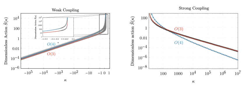
Figure 8: Fits to data of the bounce actions in the parameterization. Left: Results for the weakly coupled models, for the positive quartic potential in Eq. 11, regularized over the Thin Wall limit in Eq. 55 (), and the negative quartic, describing the BP limit in Eq. 56 (). The numerical solutions are obtained using the FindBounce Guada:2020xnz Mathematica package, regularized over the TW(BP) solution, shown as data points. The solid curve interpolates the fitted solutions for the regularized bounce . Right: Results for the strongly coupled (de)confining PT. Here, we show the bounce shape functions from Eqs. 65 and 64. Clearly, for sufficiently large the symmetric action dominates the tunneling rate, implying that quantum fluctuations drive the PT. Equipped with these results we take the approach of Ref. Adams:1993zs and numerically fit the intermediate regimes as a function of , both for positive and negative quartics (). We constrain the fit to match the known limits and require smoothness at . Starting with the positive it is useful to define the regularized functions
(58) where is the thin wall solution in (55). Close to the thin wall solution, we perform a reduced squares fit for , using the variable , optimizing over the free parameters while far away from the thin wall limit we match the fitting function smoothly to the cubic solution in Eq. 57. The resulting fitting function is
(59) where by definition the fitting function is normalized with respect to the thin wall regime. For convenience in the main text we define
(60) normalizing with respect to the pure cubic solution.
Turning to the negative regime, we perform a similar procedure, but regularizing over the BP solution in Eq. 56, as it describes the large negative limit of the full solution,
(61) These solutions are also constrained to admit the limit in order to converge with the cubic solution in Eq. 57. The fitting functions for negative are given by
(62) which asymptote to a constant, correctly describing the cubic bounce solution. Our results for match the fitting functions quoted in Sarid:1998sn , under the appropriate variable and scaling transformations, while the solutions constitute a new result. The full fitting functions are shown against the numerical solutions, obtained using the Mathematica package FindBounce Guada:2020xnz , in Fig. 8. We note that the goodness of fit for both positive and negative is at up to floating point numerical errors.
- Strong coupling
-
The bounce action for the strongly coupled theory discussed in Section IV can be written as a product of two functions, similar to the weakly coupled case, as
(63) where is a dimensionless function of . We shall appeal once more to the simple limit of , where the TW approximation is expected to hold. Here, the TW approximation for the reduced actions is given to leading order by
(64) The fitting functions are then obtained as
(65) with corresponding for respectively. The full bounce actions are then given by
(66) We note that in order to derive the nucleation temperature given in Eq. 49, one must expand the full actions in the limit of small temperature (i.e. ), and solve the nucleation condition using the following actions
(67) The nucleation temperature admits a simple form when driven by quantum fluctuations, given by
(68) This temperature is minimized at , where as in Kaplan:2006yi , resulting in Eqs. 49 and 50. A similar derivation for thermally driven transitions does not lead to an analytic expression for the nucleation temperature due to the factor which appears in Eq. 67, requiring the solution of a seventh order equation for . However, an upper bound on can still be obtained by considering the discriminant of the nucleation condition, leading to an upper bound given by .
A.2 Thermal/Quantum Tunneling at Weak/Strong Coupling
The vacuum decay rate can be dominated by either thermal or quantum fluctuations. Due to the negative exponential dependence of the tunneling rate on the bounce action, as seen from Eq. 1, it is sufficient to compare (quantum) against (thermal) to determine which one drives the PT. The lesser of the two actions at a given temperature is therefore the dominant contribution to the rate.
The two actions have different scaling with the model parameters, and potentially, either one may dominate at a different regime of coupling strengths. Here, we discuss whether nucleation proceeds via thermal or quantum tunneling for the models discussed in the main text.
- Weak coupling
-
We begin with the weakly coupled models considered in Section III. The two relevant actions are then given by Eq. 54. Since these actions must converge to the TW approximation at sufficiently high temperature, and knowing that has a double pole in , while has a triple pole in , we conclude that at , implying that high- transitions are induced by thermal fluctuations. Lowering the temperature, the condition for continued thermal dominance over quantum is simply , translated via Eq. 54 to , where the most stringent condition can be found by requiring that there exist no for which this condition is met. By inspection, the left panel of Fig. 8 demonstrates that the functions are monotonically increasing with , with their minimal value obtained at . In this limit, both actions admit simple forms given by Eq. 56, scaling as , rendering their ratio constant. The aforementioned condition for is then translated to the simple constraint
(69) This condition can be cast into the various models. For the classically scale invariant CW potential, the thermal action contribution is smaller only if the coupling strength is large . When adding a non-thermal mass, the condition is only slightly reduced, to . In the case of the non-thermal cubic addition, this condition is even easier to satisfy as the effective thermal mass can only decrease, requiring even larger values of to break Eq. 69. These results conclusively show that coupling values for which the quantum fluctuations dominate the tunneling rate are well outside the supercooling window for any of the weakly coupled models in question, and thus irrelevant.
- Strong coupling
-
We now turn to the strongly coupled model discussed in Section IV. The inequality can be written as
(70) and implies that nucleation proceeds via quantum tunneling, with the nucleation condition satisfied at . This inequality can also be written as a lower bound on the quartic
(71) where the thermal dominates for smaller . As shown in Fig. 7 within the supercooling the PT is fully controlled by quantum tunneling for a confinement scale TeV.
Appendix B Gravitational Wave Simulation Parameters
B.1 Phase Transition Temperature and Timescale
In this section we detail firstly how the correct temperature measure of the PTs completion, , changes as a function of and secondly, how this measure affects the mapping between and and therefore the predicted GW signal. It is important to recall that the definition of hinges on the assumption of exponential nucleation. For , Taylor expanding the exponent around the PT completion time defines
| (72) |
From this expansion one easily recovers the definition of (see Eq. 7) as a function of temperature. With this definition we can then assess the relevant temperature choices for :
- Nucleation temperature
-
As defined in the main body of this paper this is defined as the time-integrated probability of nucleating a single bubble per Hubble volume, which to a very good approximation is the condition .
- Percolation temperature
-
The percolation temperature is defined as the temperature where the probability of finding a point in the false vacuum falls below Coleman:1977py ; Guth:1979bh ; Guth:1981uk where the exponent can be written as (see also Ref. Azatov:2019png )
(73) The term inside the square brackets depends on the bubble wall velocity and accounts for the competition between bubble and Hubble expansion after nucleation. For fast transitions with respect to the expanding background we have .
- Temperature where false vacuum volume start decreasing
-
If the PT is delayed such that the vacuum energy of the false vacuum begins to dominate, subsequent accelerated expansion can inhibit the completion of the PT. For these slow transitions it can be necessary to use a more stringent measure for the progress of the transition; namely, requiring that the normalized volume of the false vacuum decrease as a function of time
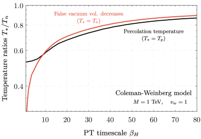
(74) where . For the case of exponential nucleation it can be shown that this translates to the requirement that Turner:1992tz , i.e this condition is more stringent than the percolation requirement at values of . This behavior is shown in the left-hand panel of Fig. 9, where the temperature ratios with respect to the nucleation temperature are shown as a function of in the context of the Coleman-Weinberg model.
To summarize the discussion of , for fast PTs or equivalently signals the completion of the transition as while for supercooled transitions , that is suffices except for extremely small values of .
With the appropriate temperature for a given identified, we must now identify the typical bubbles size at the point of their collisions. This is crucial as not only does the energy density in the bubble scale with its volume, but the majority of bubble simulations rely crucially on this measure to determine numerically the resulting GW signal. Following Ref. Turner:1992tz we can determine the size of a bubble, , at time that was originally nucleated at time as
| (75) |
The distribution of the bubble number density therefore follows as
| (76) |
Note, that the above is written as a function of time rather than temperature, which is significantly simpler for an inflating background. Assuming perfect de Sitter with scale factor we can firstly evaluate
| (77) |
Then using the relation between a bubble size at time given that it was nucleated at time
| (78) |
the bubble distribution becomes
| (79) |
There are two choices for determining a useful measure of :
- Mean bubble size
-
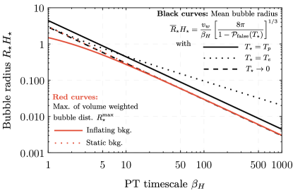
This is the most common measure used in the literature. Here we simply determine the number density of bubbles at a given time, , and use this to extract the length scale . For an inflating background we obtain
(80) Here refers to the (incomplete) Gamma functions rather than the bubble nucleation rate. Taking the large limit, i.e. the PT completes much faster than a Hubble time, yields
(81) With we recover the often used relationship between and in Eq. 8.
- Maximum of the volume weighted bubble distribution
-
As the energy density of a bubble scales with its volume, a more accurate description of the bubble size that is most pertinent to the production of GWs is through determining the maximum of the distribution in Eq. 79. This yields
(82) Interestingly, this result is independent of temperature and depends only on the size of the box and the timescale of the transition.
We summarize the results of these two choices of in Fig. 9. Shown in black is the results assuming that is large, therefore neglecting the expansion of the background, with three different choices of . While in red we show the resulting maximum of the volume weighted bubble distributions, for an inflating background (solid) and a static background/fast transition (dotted). We see that for , both red curves agree well with one another while the case with , i.e. , agrees well with defined above.
B.2 Bubble Wall Friction and Boost Factor
The final component of the PT parameters depend on the dynamics of the bubble walls during their expansion. Motivated by the results of Ref. Azatov:2019png , we use a simplified treatment for evaluating the Lorentz boost of the bubble walls at equilibrium and at the time of collision . The equilibrium scenario occurs when the leading-order pressure is balanced against the next-to-leading order emission of radiation from the bubble wall
| (83) |
where
| (84) |
The leading-order pressure is defined as the sum over all particles which gain mass in the course of the transition, where is the degrees of freedom of each species and for scalars (fermions), respectively. The next-to-leading order contribution presumes that there is vector emission (with its strength determined by coupling ) from the bubble wall with a boost-factor as the scalar field vacuum changes by an amount . The final component is the boost-factor itself at the time of bubble wall collision. Based on thin-wall approximations corroborated by numerical approaches extrapolating beyond this limit, we approximate the boost-factor as
| (85) |
See Ref. Azatov:2019png for additional details. In this expression, follows from the previous section while is the initial size of the bubbles at nucleation determined by solving the Euclidean action. We show the resulting on the same plane as earlier figures in Fig. 10 along with contours of . To summarize in Table 1 we give two representative benchmark points and the numerical values of the parameters relevant to the GW signal prediction.
| BP1 | BP2 | |
| Subsequent values evaluated at | ||
B.3 GW Simulation Parameters
To assess the detectability of a given PT, its parameters (, , and ) must be mapped to the spectrum of sourced gravitational waves. This mapping requires a combination of both lattice and magnetohydrodynamic simulations. This leads to sizeable theoretical errors, potentially larger than those of the above parameters Croon:2020cgk . As a result we make conservative assumptions when utilizing the simulation results and include only two of the possible GW generation mechanisms; bubble-wall collisions and sound waves in the plasma.777We disregard the possibility of GW generation through turbulent flows as there remain difficulties in understanding the time-scales under which the sound-wave contributions develop into turbulent flows and the subsequent loss of energy through high- modes. We will use the short-hand but often confusing notation for the total signal:
| (86) |
These two fitting functions and the additional derived quantities are given in the following subsections. Note that due to the values of in the models under consideration, the sound-wave contribution dominates over the signal generated from bubble wall collisions.
B.3.1 Bubble-wall Collisions
The latest simulations of bubble-wall sourced GWs give the following fitting functions Cutting:2018tjt [note the addition of the redshifting factor compared to Eq. (52)]
| (87) |
The redshifting factor for the GW amplitude is given by
| (88) |
with the normalized energy density in photons today being ParticleDataGroup:2020ssz , the relativistic dofs in the photon bath , and the entropy degrees of freedom at matter-radiation equality . Here we have also assumed that .
The above can be re-written in the following form
| (89) | ||||
| (90) |
with , and . More sophisticated results depending on the initial bubble wall profile are can be found in Ref. Cutting:2020nla . The scalar field generated peak frequency today is given by
| (91) | ||||
| (92) |
The last piece is the energy fraction that the bubble wall carries .
| (95) |
The above expressions are taken from Ref. Azatov:2019png . Here, is the boost-factor whereby the friction effects (both leading and next-to-leading order) balance against the energy released in the PT, while is the approximate boost of the bubble walls at percolation. Lastly, , i.e. the size of the leading order friction effects normalized to the energy density in the radiation bath.
B.3.2 Sound-wave Contribution
We use the most up-to-date expression from fitting acoustic sound-wave simulations, making comparisons to other works in the literature. Starting from the corrected expression, Eq. (2), in the erratum of Ref. Hindmarsh:2017gnf the sound-wave contribution to the GW signal is
| (96) |
For comparison to other works and to aid in navigating the diverse confusing array of notation used in the literature, we concretely take (valid for a relativistic plasma), as suggested from simulations (c.f Ref. Hindmarsh:2017gnf ) and
| (97) |
The peak frequency for the sound wave spectrum is
| (98) |
while the efficiency factor is
| (101) |
Based on the determination of the boost factor at the percolation time (following Ref. Azatov:2019png ) we find that , which from Ref. Espinosa:2010hh gives
| (102) |
The above can be rewritten in terms of and a modified shape function utilized in Ref. Craig:2020jfv
| (103) | |||
| (104) |
This yields (for the case where )
| (105) | ||||
| (106) |
where the numerical coefficient differs from Eq. (2.25) of Ref. Craig:2020jfv by approximatel a factor of 2.
We also compare our results with Ref. Azatov:2019png . Defining [according to their definition below Eq. (41)] and explicitly substituting in yields
| (107) | ||||
| (108) |
This result is over an order of magnitude smaller than the result in Eq. (39) of Ref. Azatov:2019png , namely a numerical prefactor of that likely arises from a typo in their definition of (as this was updated in the erratum of Ref. Hindmarsh:2017gnf ).
Appendix C Gravitational wave experimental noise curves and signal-to-noise ratios
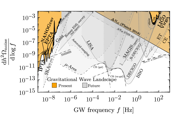
To assess the detectability of a given PT signal we adapt a frequentist approach following closely appendix B of Ref. Breitbach:2018ddu . We express the signal-to-noise ratio in the following form
| (109) |
where is the PT signal from Appendix B and is the effective noise curve of a single detector or network of detectors. This effective noise curve is derived using
| (110) |
where , are the overlap reduction functions which depend on the network of detectors considered (here we follow the derivation from Appendix A.2 in Ref. Schmitz:2020syl ) and is the noise curve for an individual detector. The final missing components are the values for the observation time , , and the signal-to-noise threshold which are given in Table 2. For future observatories we have used a signal-to-noise threshold of 10 unless otherwise stated in the projection papers, while for PTAs noise curves are often not given, hence the threshold is reverse-engineered (see Appendix B of Ref. Breitbach:2018ddu ). The multiplicative factor is determined by the presence of more than one detector to allow for cross-correlations in the signal searches.
In Fig. 11 we show the resulting effective noise curves . Current experiments are shaded as orange regions while future experiments are shaded in grey with varying line styles. Lastly, the expected astrophysical backgrounds are given be black dot-dashed lines. These are the super-massive binary black-hole background (SMBHB), compact binary mergers (CB) from both galactic (gal) and extra-galactic (ex-gal) sources which form an unresolvable stochastic background Farmer:2003pa ; Cornish:2017vip ; Robson:2018ifk . Also shown on Fig. 11 are bounds arising from measurements where the energy density in GWs is behaving like extra radiation during the CMB and BBN epochs. The comparison here with dedicated GW experiments is possible only through the assumption of a signal shape, namely we have assumed the shape to be delta function of a given frequency and amplitude. This is a good approximation to the typical broken power-laws of the PT GW signals as the energy density in GWs is dominated by the relatively narrow peak in the spectrum. Recall however, that GW experiments can detect signals with amplitudes at least one order of magnitude smaller their respective noise curves. To that end in Fig. 12 we also show the sensitivity to a mock phase transition signal based on the BP1 of Table 1, where we simply shift the signals peak frequency and amplitude. Here we see explicitly that the LIGO/VIRGO sensitivity is comparable to measurements.
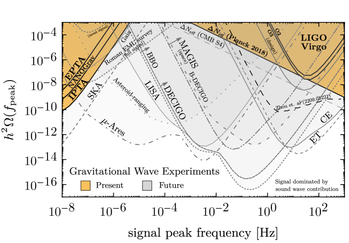
| Experiment | and | |||
| Ground-based GW interferometers | ||||
| LIGO/Virgo O2 | 150 days | 10 | 2 | Taken from Ref. Schmitz:2020syl based on public data LHO:2017aaa ; LLO:2017aaa ; Virgo:2017aaa |
| LIGO/Virgo O3 | 11 months | 10 | 2 | Network sens. based on method in Schmitz:2020syl , data from LIGOScientific:2021djp (Fig. 2 from Virgo:2022aaa ) |
| LIGO/Virgo/KAGRA Design | 2 yrs | 10 | 2 | Same as above, data from KAGRA:2013rdx |
| ET | 5 yrs | 5 | 1 | ET-D configuration from Fig. 4 of Sathyaprakash:2012jk |
| CE | 5 yrs | 5 | 1 | Wide-band projection from Fig. 2 of LIGOScientific:2016wof |
| Space-based GW experiments | ||||
| LISA | 4 yrs | 10 | 1 | Eq. 13 of Robson:2018ifk |
| BDECIGO | 4 yrs | 8 | 1 | Fig. 1 of Isoyama:2018rjb |
| DECIGO | 4 yrs | 10 | 2 | Fig. 2 of Yagi:2013du |
| BBO | 4 yrs | 10 | 2 | Fig. 1 of Yagi:2011yu based on Harry:2006fi |
| AION/MAGIS space | 5 yrs | 5 | 1 | Fig. 1 of Graham:2017pmn (see also Graham:2016plp ; Badurina:2019hst ) |
| -Ares | 10 yrs | 10 | 1 | Fig. 5 of Sesana:2019vho |
| Astrometric and pulsar timing | ||||
| Asteroid-ranging | 10 yrs | 10 | 2 | Optimistic projection from Fig. 5 of Fedderke:2021kuy |
| GAIA | 5 yrs | 10 | 2 | Fig. 3 of Wang:2020pmf (based on Klioner:2017asb ; Moore:2017ity ) |
| Roman EML survey | 5 yrs | 10 | 2 | Fig. 3 of Wang:2020pmf (mean and full signal subtraction shown) |
| NANOGrav | 11 yrs | 0.696 | 2 | Extracted from NANOGRAV:2018hou (see App. B of Breitbach:2018ddu ) |
| EPTA | 18 yrs | 1.19 | 2 | Extracted from Lentati:2015qwp ; Desvignes:2016yex (see App. B of Breitbach:2018ddu ) |
| SKA | 10 yrs | 4 | 2 | From projections in App. B of Breitbach:2018ddu based on Janssen:2014dka ; Weltman:2018zrl |
| IPTA | 18 yrs | 4 | 2 | Central value measurements from Fig. 1 of Antoniadis:2022pcn |
| Cosmology | bound | |||
| Planck 2018 | Recast performed in Opferkuch:2019zbd based on Planck:2018vyg | |||
| CMB Stage 4 | Recast performed in Opferkuch:2019zbd based on CMB-S4:2016ple | |||