Mod-Squad: Designing Mixture of Experts As Modular Multi-Task Learners

Abstract

Optimization in multi-task learning (MTL) is more challenging than single-task learning (STL), as the gradient from different tasks can be contradictory. When tasks are related, it can be beneficial to share some parameters among them (cooperation). However, some tasks require additional parameters with expertise in a specific type of data or discrimination (specialization). To address the MTL challenge, we propose Mod-Squad, a new model that is Modularized into groups of experts (a ‘Squad’). This structure allows us to formalize cooperation and specialization as the process of matching experts and tasks. We optimize this matching process during the training of a single model. Specifically, we incorporate mixture of experts (MoE) layers into a transformer model, with a new loss that incorporates the mutual dependence between tasks and experts. As a result, only a small set of experts are activated for each task. This prevents the sharing of the entire backbone model between all tasks, which strengthens the model, especially when the training set size and the number of tasks scale up. More interestingly, for each task, we can extract the small set of experts as a standalone model that maintains the same performance as the large model. Extensive experiments on the Taskonomy dataset with 13 vision tasks and the PASCAL-Context dataset with 5 vision tasks show the superiority of our approach.

1 Introduction

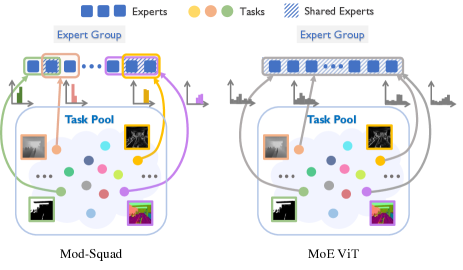
Figure 1: A comparison between Mod-Squad and MoE ViT. Our key motivation is that experts should leverage commonalities in some tasks (cooperation) but focus on a subset of tasks that require specific features and do not interfere with each other (specialization).

Computer vision involves a great number of tasks including recognition, depth estimation, edge detection, etc. Some of them have a clear and strong relationship: they are likely to benefit from shared features. An example would be a task to classify cars and pedestrians and a task to segment the same classes. Other tasks appear to be less related: it is not clear what features they would share. An example could be tumor detection in medical images and face recognition.

Multi-task learning (MTL) aims to model the relationships among tasks and build a unified model for a diverse set of tasks. On the one hand, tasks often benefit by sharing parameters, i.e., cooperation. On the other hand, some tasks may require specialized expertise that only benefits that single task, i.e., specialization. A good MTL system should be flexible to optimize experts for the dual purposes of cooperation and specialization.

There are two well-known challenges in MTL: (1) gradient conflicts across tasks [5, 38]; and (2) how to design architectures that have both high accuracy and computational efficiency. Previous efforts include manually designing architectures [4] or conducting neural architecture search [1] to induce cooperation and specialization in different parts of the model. However, these methods either require heavy manual customization, reducing generality and limiting applicability, or require very long training times.

To address these challenges, we introduce Mod-Squad, a new model that constructs a Mixture of Experts (MoE) [31] to be modularized multi-task learners (a squad). Our design allows experts to cooperate on tasks when it is helpful, rather than penalizing experts that do not participate in every task. At the same time, some experts naturally develop a deep specialization in particular tasks, improving performance. The left figure in Fig. 1 shows an example of the specialization and cooperation of experts in Mod-Squad. A further and important side benefit, discussed below, is that this sparsification of experts allows our model to be decomposed into much smaller single-task models that perform extremely well.

We achieve these goals by first integrating mixture of experts (MoE) layers into our vision transformer [6] backbone network. The motivation is to divide the model into groups of experts, and for each expert to construct a minimum part of the model that can be shared among tasks or be specialized for one task. The experts can have any network structure (e.g., MLP or attention network [40]) so that we can incorporate advanced model designs. Our modular design allows cooperation and specialization via the distribution of tasks to experts and also experts to tasks. Below, we formalize this idea mathematically by analyzing the probability distribution over tasks and experts, and using a novel loss function to induce a specific structure on this distribution.

Many previous MoE works [31, 29, 40] use a load-balancing loss that encourages the frequency of expert usage (across all tasks and batches) to be highly similar. Some MoE methods [18, 26] directly apply this loss after the forward pass of each task on the multi-task scenario so that each task evenly uses all experts. However, this approach may force experts to set parameters on conflicting tasks with learning gradients that counteract each other. In other words, while an expert may benefit from being shared among certain pairs of tasks, it may be harmed by being forced to share among other pairs of tasks. This is an explanation for the difficulty of training multi-task models under such an expert-balancing loss.

In comparison, we contend that experts should leverage commonalities in some tasks (cooperation) but also create a subset of experts that learn specific features (as needed by some tasks) and do not interfere with each other (specialization). Such an assignment of tasks to experts can be represented via a sparse but strong dependence between experts and tasks. Fig. 1 illustrates this key difference between our model and previous MoE work, showing how our model induces a sparser structure in the assignment of experts to tasks. To implement this idea, we add a loss term to maximize the mutual information between experts and tasks. This induces a strong dependency between experts and tasks, with each task heavily related to a small set of experts and vice versa.

Interestingly, we find that our model converges to a state in which, after training, most experts are never or rarely used for many tasks (evidence of specialization), but the experts are still balanced in their activation frequency. This property enables us to extract a compact sub-network from the giant model for each task. The small networks extracted in this fashion work independently as standalone models for individual tasks with no performance drop. This property enables us to train a giant, sparse model in a scaled-up multi-task learning scenario and later get compact sub-networks for each task with high performance.

Our main contributions can be summarized as follows:

• Modular multi-task learner. We propose a new modular backbone model, Mod-Squad, that is composed of a large group of attention and feed-forward experts. The experts can be flexibly assigned a subset of tasks to achieve specialization and cooperation.

• Optimizing the joint distribution over tasks and experts. Mod-Squad includes a new loss term that encourages a sparse but strong dependence between experts and tasks. This is done by measuring and maximizing the mutual information between tasks and experts.

• Effective and Efficient multi-task learners at scale. Experiment results show that Mod-Squad achieves state-of-the-art performance on two major multi-task datasets while maintaining its computational efficiency.

• Extracting small sets of experts as standalone models with no performance drop. We further show that Mod-Squad can be effectively pruned for a designated task without sacrificing performance.

2 Related Work

Multi-task Learning. Multi-task learning jointly learns multiple tasks by sharing parameters among tasks. One common approach is to manually design the architecture, sharing the bottom layers of a model across tasks [4, 14, 2]. Some works [34] design the architecture according to task affinity. Others [1, 2, 32] leverage Neural Architecture Search or a routing network [30] to learn sharing patterns across tasks and automatically learn the architecture. Recently, transformer-based MTL architectures [36] have been explored and have shown advantages over CNN-based models. In comparison, we customize MoE layers into vision transformers; each MoE module constructs a minimum part of the model that can be distributed to a subset of all tasks instead of all tasks. As a result, our model is flexible in its creation of cooperation and specialization.

Mixture of Experts (MoE). The MoE was first proposed by Jacobs et al. [12] as a technique to combine a series of sub-models and perform conditional computation. Recent work [31] in NLP proposes sparse MoE to reduce computation cost, and some works [15, 8] train gigantic models with trillions of parameters based on the sparse model. Some have used the MoE technique to train huge models in vision [29, 35] or multi-modal applications [26]. These works typically focused on combining the Feed-Forward Network layer with the MoE or develop a better routing strategy [16, 27]. MoA [40] proposes a new module that combines the attention network with the MoE while having a low computational cost and the same parameter budget as a regular attention network. More recently, M³ViT [18] uses MoE techniques to design a multi-task learning model that is computationally efficient during training. Compared to these previous methods, we demonstrate a MoE model that is not only computationally efficient, but is also flexible as a modularized multi-task learner that can easily induce both cooperation and specialization. Although M³ViT [18] also use MoE in their approach, the experts in their model share between all tasks and cannot be specialized for tasks.

Pruning. Pruning refers to the process of removing components of a larger model to produce a smaller model for inference, with the goal of maintaining as much accuracy as possible while improving runtime computation efficiency. Generally, pruning is categorized into unstructured pruning [10], which removes individual weights that have a minimal contribution to accuracy and structured pruning [11, 17], which ranks filters or blocks and prunes these based on some criterion. Usually, extra fine-tuning is conducted for the pruned network to help maintain the performance [28, 20, 37]. Most of pruning is for single task and very few of them consider the case in multi-task learning. In this work, our proposed model has a unique property that a series of small sub-network for each task can be extracted from it with no performance drop and no additional fine-tuning. This is somehow similar to pruning but more likely to be an advantage of our model rather than a new way of pruning.

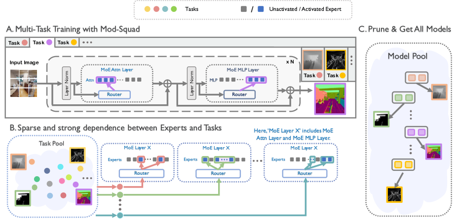
Figure 2: The pipeline of our multi-task foundation model. Each transformer block in Mod-Squad consists a MoE attention network (MoE attn.) and a MoE MLP network. The multi-task model Mod-Squad is trained with our proposed mutual information loss. Mod-Squad develops a strong dependence between experts and tasks. Then we can extract a small sub-network from Mod-Squad for each task with no performance drop.

3 Method

We start with the definition of multi-task learning. Suppose we have $M$ tasks $T_{1},T_{2},...,T_{M}$ and $Q$ images $I_{1},I_{2},...,I_{Q}$. We define a task $T$ as a function that maps image $I_{q}$ to $T(I_{q})$. Our dataset $D$ contains for each task $T_{i}$ a set of training pairs $(I_{q};T_{i}(I_{q}))$, e.g. (image; depthMap). Here, for simplicity, we assume that every task contains a training pair for every one of the $Q$ images, but note that our approach can be extended to the case in which every task contains a different subset of images in its training pairs.

3.1 Preliminaries

Mixture of Experts. A Mixture of Experts (MoE) layer typically contains a set of expert networks $E_{1},E_{2},...,E_{N}$ along with a routing network $G$. The output of a MoE layer is the weighted sum of the output $E_{k}(x)$ from every expert. The routing network model $G$ calculates the weight $G^{k}$ for each expert given input $x$. Formally, the output of a MoE layer is

$$y= \sum_{k=1}^{N}G^{k}(x)E_{k}({x}).$$ (1)

The routing network $G$ is a Noisy Top-$K$ Routing network [31] with parameters $W_{g}$ and $W_{noise}$. It models $P(E_{k}|x)$ as the probability of using expert $E_{k}$ and selects the Top-$K$ to contribute to the final output. The whole process is shown as follows:

$$G(x)= \operatorname{TopK}(\operatorname{Softmax}(xW_{g}$$

$$+\mathcal{N}(0,1)\operatorname{Softplus}(xW_{noise}))),$$ (2)

where $\operatorname{TopK}(\cdot,k)$ sets all elements in the vector to zero except the elements with the largest $K$ values, $\operatorname{Softplus}$ is the smooth approximation to the ReLU function:

$$\operatorname{Softplus}(x)= log\left(1+\exp\left(x\right)\right).$$ (3)

3.2 Mod-Squad

Mod-Squad is a multi-task model with the vision transformer as the backbone network and several parallel task-specific heads. As shown in Fig. 2, a key design in our model is customizing MoE into the vision transformer so that each expert can construct a minimum part of the model that can be either shared between tasks or specialized for tasks. Specifically, we customize the MoE attention block (MoA) [40] and MoE MLP block [31] into the transformer layer. Each MoE block consists of $N$ experts $E_{1},E_{2},...,E_{N}$ which can be either an attention head or an MLP layer along with $M$ task-specific routing networks $G_{1},G_{2},...,G_{M}$ that select experts conditioned on input tokens. Note that each routing network $G_{i}$ has its own parameters $\left(W_{g}^{i},W_{noise}^{i}\right)$. We also add a learnable task embedding to the hidden input state so that each expert is aware of the target task. Thus, in Mod-Squad, the output of each MoE layer is

$$y=\sum^{N}_{k=1}G^{k}_{i}(x)\cdot E_{k}\left(x+e_{i}\right),$$ (4)

where $i$ is the task id and $e_{i}$ is the respective task embedding.

3.3 A joint probability model over tasks and experts

In order to model cooperation and specialization, we define a probability model over tasks $T$ and experts $E$. We assume that when our trained network is deployed, it will be assigned a random task $T$ according to a global distribution over tasks $P(T)$. (Typically we assume this distribution to be uniform over tasks.) Subsequently, it will be given a random image $X$ according to $P(X|T)$.

For a given MoE layer, we model the probability $P(E_{i}|T_{j})$ of using expert $E_{i}$ with task $T_{j}$ as the frequency with which $E_{i}$ is assigned to task $T_{j}$ by the routing network. For example, for 100 images in task $T_{j}$, if the routing network assigns 30 of them to expert $E_{i}$, then $P(E_{i}|T_{j})=0.3$. Since the routing network does not make hard assignments of experts to tasks, but rather assigns weights resulting from a softmax function to each expert, we sum these soft weights to measure the frequency:

$$P(E_{i}|T_{j})=\sum_{k=1}^{Q_{T_{i}}}G_{T_{j}}^{E_{i}}(x_{k}),$$

where $G_{T_{j}}^{E_{i}}$ gives the weight for expert $E_{i}$ for task $T_{j}$ on the input $x_{k}$ from image $I_{k}$. $Q_{T_{i}}$ is the number of images for task $T_{i}$. Given this definition of conditional probability, the joint probability $P(E,T)=P(E|T)P(T)$, and of course, we can obtain $P(E)=\sum_{T}P(E,T)$.

A key intuition in our work is that experts should be dependent on tasks, that is, experts should specialize in specific tasks, at least to some extent. This notion can be captured by measuring the mutual information (MI) between tasks and experts, using the probability model defined above:

$$I(T;E)= \sum_{i=1}^{M}\sum_{j=1}^{N}P(T_{i},E_{j})\log\frac{P(T_{i},E_{j})}{P(T_{i})P(E_{j})}.$$ (5)

If experts are assigned with equal frequency to all tasks, then the mutual information will be 0. If each expert is assigned to exactly one task (when $M=N$), then the dependence (and hence the mutual information) is maximized.

3.4 Maximize mutual information between experts and tasks

To understand what mutual information do, we break down the Equation. 5 as following:

$$I(T;E)= \sum_{i=1}^{M}\sum_{j=1}^{K}P(T_{i},E_{j})\log P(T_{i},E_{j})$$

$$-\sum_{i=1}^{M}P(T_{i})\log P(T_{i})$$

$$-\sum_{j=1}^{K}P(E_{j})\log P(E_{j}).$$ (6)

In Eq. 3.4, the first term is the negative entropy of $P(T_{i},E_{j})=P(E_{i}|T_{j})P(T_{j})$. Maximizing this term encourages the sharpness of the conditional distributions $P(E_{i}|T_{j})$, since $P(T_{j})$ is a constant decided by data distribution, and is not affected by model parameters. The second term is the entropy of $P(T_{i})$ which, again, is a constant and can be ignored. The third term is the entropy of $P(E_{j})$. Maximizing the term encourages a high-entropy or flat distribution of $P(E_{j})$, encouraging the experts to be evenly used across the entire dataset.

In practice, we add $-I(T;E_{Y})$ to our total loss for each MoE layer $Y$ with a weight parameter $w_{MI}$ where $E_{Y}$ represents all the experts in $Y$. We follow [13] to learn an auto-balancing weight $w_{T}$ for each task $T$ and add the task-specific loss $L_{T}$ for all tasks. So the total loss is

$$\mathtt{L}=\sum^{M}_{i=1}w_{T_{i}}L_{T_{i}}-w_{MI}\sum_{\forall MoE\ \mathtt{layers}\ Y}I(T;E_{Y}).$$ (7)

3.5 Train Once and Get All

In previous MoE works[18, 26], they use a subset of the experts for one input image but all the experts for each task. In comparison, Mod-Squad activates a subset of the experts when forwarding both single image and multiple images from the same task. Further, all the experts are evenly used in Mod-Squad when forwarding the whole multi-task dataset. This guarantees that the capacity of Mod-Squad is fully utilized and not wasted. A typical relation between tasks and experts will be demonstrated in Sec. 4.3.

Benefiting from the constant sparsity of Mod-Squad at the image-level and the task-level, unused or rarely used experts can be removed in each MoE module when doing single-task inference. This can be done by counting the using frequency of each expert for the task and removing those experts with smaller frequency than a threshold $\theta$. Note that some tasks could use more experts and others use less for each MoE layer. For example, a low-level task may require more experts at the first few layers of the network and a high-level task may require more experts at the last few layers of the network. Mod-Squad is capable of dynamically self-organize architecture and selecting experts according to the requirement of tasks, which provides some degree of freedom in architecture and extra flexibility in allocating model capacity.

After removing experts, our pruned model can be directly deployed for the respective task. Since the removed experts are never or rarely used, the pruned model achieves the same level of performance as the original model but with a much smaller number of parameters and without any fine-tuning. In the case where we set $\theta=0$ and keep all the experts that have ever been used, we observe no drop in performance while still effectively pruning a large portion of the model. This removing experts process is similar to pruning, but we just adapt a simple thresh then remove strategy and no additional training is needed like in some of the pruning work[3]. Once training, a series of small sub-networks can be extracted for all tasks. This property enables us to build a very large model benefit from all tasks, but only requires a fraction of model capacity for single-task inference or fine-tuning.

4 Experiment

Model	Obj. Cls.	Scene Cls.	Depth Euc.						Normal	Curvature	Reshading	Edge3D	Keyp.2D	Segm.2D
	$Acc(\%)\uparrow$	$Acc(\%)\uparrow$	$RMSE\downarrow$	Error $\downarrow$		$\delta$, within $\uparrow$			L1 dis. $\downarrow$	L2 dis. $\downarrow$	L1 dis. $\downarrow$	L1 dis. $\downarrow$	L1 dis. $\downarrow$	L1 dis. $\downarrow$
				Abs.	Rel.	1.25	$1.25^{2}$	$1.25^{3}$
STL	56.5	60.0	6.94	0.089	1.77	92.8	96.9	98.7	0.403	1.12	0.184	0.119	0.0312	0.171
MTL	57.3	64.9	6.75	0.084	1.26	93.0	97.0	98.9	0.386	1.06	0.170	0.127	0.0284	0.166
$M^{3}ViT$[18]	58.0	65.6	6.69	0.083	1.26	93.2	97.2	98.9	0.383	1.05	0.174	0.126	0.0289	0.164
Mod-Squad	59.0	66.8	6.59	0.082	1.25	93.3	97.2	99.0	0.374	1.02	0.167	0.123	0.0275	0.161

Table 1: Metric for each task on the taskonomy dataset. For each task, we use different metrics to evaluate its performance. More results on other tasks can be found in the supplementary.

Method	STL	MTL	M3ViT	MLP	Attn	Ours	Pruning
Params(M)	86.4	90.0	176.4	176.4	105.6	201.3	116.9
FLOPs(G)	17.7	18.5	19.7	19.7	19.7	19.7	18.4
Object Cls.	0.0	+1.4	+2.6	+3.0	+3.0	+4.4	+4.4
Scene Cls.	0.0	+8.1	+9.3	+10.0	+9.6	+11.3	+11.3
Depth Euc.	0.0	+2.7	+3.6	+3.9	+4.4	+5.0	+5.0
Depth Zbu.	0.0	+2.1	+2.4	+2.6	+2.4	+2.8	+2.8
Normal	0.0	+3.5	+4.2	+4.5	+4.5	+6.5	+6.5
Curvature	0.0	+5.3	+6.2	+7.1	+6.2	+8.9	+8.9
Reshading	0.0	+7.6	+5.4	+5.9	+8.1	+9.2	+9.2
Edge2D	0.0	+0.6	+2.0	+1.8	+1.2	+3.6	+3.6
Edge3D	0.0	-6.7	-5.8	-4.2	-5.8	-3.3	-3.3
Keyp.2D	0.0	+5.3	+3.6	+3.6	+6.3	+8.3	+8.3
Keyp.3D	0.0	+1.3	+2.7	+4.1	+2.7	+5.5	+5.5
Segm. 2D.	0.0	+2.9	+4.0	+5.2	+3.5	+5.8	+5.8
Segm. 2.5D	0.0	+1.9	+3.2	+3.8	+3.2	+5.1	+5.1
Mean	0.0	+2.8	+3.3	+3.9	+3.8	+5.6	+5.6

Table 2: Comparison of $\Delta_{t}$ between MTL methods on the Taskonomy. We report their average drop for each task with respect to the vanilla single-task model. MLP and Attn represent using only MoE MLP and MoE attention network in the backbone respectively.

4.1 Experiments Settings

Datasets and Tasks. We evaluate on two multi-task datasets: PASCAL-Context[25] and Taskonomy[39]. The PASCAL-Context includes 10,103 training images and 9,637 testing images with the five task annotation of edge detection (Edge), semantic segmentation (Seg.), human parts segmentation (H.Parts), surface normals (Norm.), and saliency detection (Sal.). The Taskonomy benchmark includes 3,793k training images and 600k testing images with 16 types of annotation. We use 13 annotations among them as our multi-task target: object classification, scene classification, depth estimation with euclidean depth, depth estimation with z-buffer depth, surface normals, curvature estimation, reshading, edge detection in 2D and 3D, keypoint detection in 2D and 3D, unsupervised segmentation in 2D and 2.5D. Details of these tasks can be found in [39].

Loss Functions and Evaluation Metrics. Classification tasks and semantic segmentation use cross-entropy loss and pixel-wise cross-entropy loss respectively. Surface normals calculate the inverse of cosine similarity between the l2-normalized prediction and ground truth. Curvature estimation uses L2 loss. All other tasks use L1 loss.

We follow previous work [23] to use $\Delta t_{i}$ to evaluate a MTL model $m$ as the average drop for task $T_{i}$ with respect to the baseline model $b$: $\Delta t_{i}=(-1)^{s_{i}}(M_{m,i}-M_{b,i})/M_{b,i}$ where $M_{m,i}$ and $M_{b,i}$ are the metrics of task $T_{i}$ for the model $m$ and $b$ respectively, and $s_{i}$ is $1$ if the metric is the lower the better and $0$ otherwise. We also report $\Delta t$ as the average of $\Delta t_{i}$ on all tasks. For here, the baseline model $b$ is the vanilla single-task learning model.

On the taskonomy, for depth estimation, we also report root mean square error (rmse), absolute and relative errors between the prediction and the ground truth as well as the percentage of pixels whose prediction is within the thresholds of $1.25,1.25^{2},1.25^{3}$ to the ground truth following [7]. We also report accuracy (Acc) for classification, L2 distance for curvature estimation, and L1 distance for all other tasks. These metrics are used to calculate $\Delta t_{i}$ and note that depth estimation use rmse only.

On the PASCAL-Context, we follow [18] and report mean intersection over union (mIoU) for semantic and human parts segmentation, and saliency; mean error (mErr) for normals estimation, root mean square error (rmse) for depth estimation; and optimal dataset F-measure (odsF) for edge detection.

Baselines and Competitors. We compare with the following baselines. STL: vanilla single-task learning baseline that trains its own model on each task independently. MTL: vanilla multi-task learning baseline that all tasks share the backbone model but have separate prediction heads. For our proposed model, we also have MLP and Attn (in Table. 2) that represent only MoE MLP and only MoE attention networks are customized into the transformer layer respectively. Mod-Squad w/ pruning (or pruning in Table. 2) is Mod-Squad with experts removing for each specific task and we report the maximum FLOPs and Params over all tasks. We also compare with $M^{3}ViT$[18] and several state-of-the-art MTL models: MTAN[19], Cross-Stitch [24] and NDDR-CNN[9]. Further, we compare with modified-MoE: it has the same architecture as Mod-Squad but without our mutual information loss. It applies the standard balanced loss [40] after forward propagation of all tasks for each image instead of one task. As a result, experts will be evenly used for all tasks instead of for every task.

Implementation. We use ViT-base[6] and ViT-small as backbone networks on the Taskonomy and the PASCAL-Context respectively. We introduce MoA and MoE MLP into ViT every two layers. For MoA, we follow [40] to design the block and use 15 experts with top-k as 6 for ViT-small and 24 experts with top-k as 12 for ViT-base. For MoE MLP, we use 16 experts with top-k as 4. The task-specific heads are single linear layers on the Taskonomy and multiple layers network same as [18] on the PASCAL-Context. We set $w_{MI}=0.001$ and removed threshold $\theta=1.0\%$.

On the PASCAL-Context, the hyperparameters are the same as in $M^{3}ViT$[18]. On the Taskonomy, we set the base learning rate to $2e-4$ with a batch size of $1,440$ and AdamW[22] as the optimizer. The weight decay is $0.05$. We use 10 warmup epochs with 100 total training epochs and the model converges in 80 hours with 240 NVIDIA V100 GPUs. Cosine decay[21] is used for the learning rate schedule.

Method	Backbone	Seg.	Norm.	H. Parts	Sal.	Edge	$\Delta_{t}$	FLOPs	Params
		mIoU$\uparrow$	mErr$\downarrow$	mIoU$\uparrow$	mIoU$\uparrow$	odsF$\uparrow$	(%)$\uparrow$	(G)$\downarrow$	(M)$\downarrow$
STL	ResNet-18	66.2	13.9	59.9	66.3	68.8	0.00	1.8	11
MTL	ResNet-18	63.8	14.9	58.6	65.1	69.2	$-$2.86	1.8	11
MTAN[19]	ResNet-18	63.7	14.8	58.9	65.4	69.6	$-$2.39	1.8	11
Cross-Stitch [24]	ResNet-18	66.1	13.9	60.6	66.8	69.9	+0.60	1.8	11
NDDR-CNN[9]	ResNet-18	65.4	13.9	60.5	66.8	69.8	+0.39	1.8	11
MTL	ViT-small	70.7	15.5	58.7	64.9	68.8	$-$1.77	4.6	21
$M^{3}ViT$[18]	MoE ViT-small	72.8	14.5	62.1	66.3	71.7	+2.71	5.2	42
Mod-Squad	MoE ViT-small	74.1	13.7	62.7	66.9	72.0	+4.72	5.2	50
Mod-Squad w/ Pruning	MoE ViT-small	74.1	13.7	62.6	66.9	71.9	+4.65	5.2	22

Table 3: Quantitative Results on the PASCAL-Context. Mod-Squad constantly outperform other MTL methods on all tasks.

4.2 Results on MTL

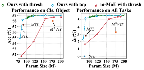
Figure 3: Ablation study on pruning. We explore two ways of pruning: (1) thresh then remove with $\theta$ (2) Keep the top $H\%$ experts that have the highest used frequency in each MoE module. For the first way of pruning, we report results with $\theta$ as 90%, 50%, 20%, 5%, 0.1%, and 0.0% (no pruning). For the second way of pruning, we report results with $H\%$ as 30%, 40%, 60%, 80%, and 100% (no pruning). We also compare our pruning with applying the same pruning strategy on modified-MoE (m-MoE).

Efficacy. We demonstrate the efficacy of our model in performance, computation cost, and model capacity. The results on the Taskonomy and the PASCAL-Context are shown in Table. 2 and Table. 3 respectively. Specific metrics for each task on the Taskonomy is shown in Table. Appendix. In terms of performance, our method significantly outperforms other baselines and competitors on both datasets: we beat MTL and M³ViT for over 2 points in mean $\Delta_{t}$ on the two datasets. On Taskonomy, we defeat MTL on all tasks, which proves the improvement is consistent. In terms of computation cost and model capacity, our model with ViT-Base backbone has a very low computation cost (19.7G FLOPs) while benefiting from a huge model capacity (201.3M). In comparison, MTL baselines with ViT-Base use 18.5G FLOPs with 86.4M parameters. Furthermore, our standalone pruned model keeps the same performance as Mod-Squad for each individual task when having the same level of computation cost and model capacity as STL: 18.4 FLOPs vs. 17.7 FLOPs and 116.9M vs. 86.4M. The extra computation cost is mainly from the lightweight routing network and the extra parameters can be further removed with a higher $\theta$ as will be shown later.

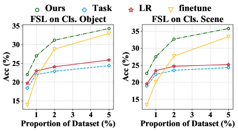
Figure 4: Router fine-tuning can quickly learn new tasks by selecting proper experts. We train our model on the other 11 tasks from the Taskonomy and transfer to cls. object and cls.scene with few training samples. We compare the few-shot classification accuracy with the following three baselines. (1) Fine-tuning: We fine-tune the whole model on the few training samples. (2) Task: we freeze the backbone model and only train the new task-specific head. (3) LR: the state-of-the-art few-shot learning method [33] based on logistic regression. We report the test accuracy when training with 0.5%, 1%, 2%, and 5% of the training set.

Ablation study on MoE Mlp and MoE Attention. As shown in Table. 2, we report results (MLP and Attn in Table. 2) where we only introduce MoE into MLP and attention networks. Both ways of adding experts can improve $>1.0\%$ in $\Delta_{t}$ compared to MTL. By combining them, Mod-Squad gets the best result and further boost 2 points in $\Delta_{t}$. This demonstrates that introducing MoE and increasing model capacity in both attention and MLP network can increase the performance.

4.3 Experts, Tasks, and Pruning

Relation between experts and tasks. As shown in Fig. 5, we visualize the frequency of experts being selected for each task. The x-axis and y-axis represent experts and tasks respectively. Experiments are conducted on the Taskonomy with all 13 tasks using MoE ViT-Small as the backbone. The visualization is for the MoE attention module in the 6th transformer block. We also compare with modified-MoE and Normal MoE which have different MoE losses but the exact model architecture. From the figure, we observe that our expert activation map is sharper and more sparse than the two comparisons, which aligns with our key motivation: a sparse but strong dependence between experts and tasks helps MTL.

Extracting sub-network for an individual task. As introduced in Sec. 3.5, we extract a small sub-network from Mod-Squad for an individual task. Specifically, we explore two ways of removing experts as follows. (1) Thresh and remove: we simply remove all experts that have an usage frequency lower than $\theta$ for the specific task. Note that some MoE modules could have fewer than Top-K experts after removing if most of the experts have a low usage frequency. In that case, we reduce the top-k of that MoE module to the number of experts it keeps. (2) Keep the top: we keep the top $H\%$ experts in each MoE module that have the highest usage frequency.

The results are shown in Fig. 3. For the first way of removing experts, we try $\theta$ as 90%, 50%, 20%, 5%, 0.1%, and 0% (no removing). For the second way, we try $H\%$ as 50%, 20%, 5%, and 0% (no removing). For both removing strategies, we compare with STL, MTL, and M³ViT. From the figure, we notice several interesting observations: (1) Mod-Squad can remove the majority of extra experts than a normal ViT-Base (116.9M vs. 90.0M in model parameters) with a tiny performance lost ($<0.3\%$ in $\delta_{t}$) and still better than competitors. (2) Only keeping the top 40% of experts still give us the same performance (5.5% in $\delta_{t}$ while the best is 5.6%). (3) The performance of modified-MoE significantly drops when removing more experts, which prove the effectiveness of our mutual information loss.

Fine-tuning the router network. Another interesting property of Mod-Squad is that we can quickly adapt to new tasks by only tuning the lightweight routing network and the task-specific head with all other parameters frozen. We refer to this technique as router fine-tuning. Router fine-tuning can be generalized to any MoE network when they need lightweight tuning with limited budgets in dataset size, computation cost, or training time.

As shown in Fig. 4, we explore router fine-tuning. We first pre-train our model on 11 tasks on the Taskonomy except for cls. object and cls. scene as the target of new tasks. We compare different ways of fine-tuning with limited training examples. We report performance using 0.5%, 1%, 2%, and 5% of the dataset to learn the new tasks. The router fine-tuning strategy is compared with several baselines as follows. (1) Fine-tuning: fine-tune the whole model and learn the new task-specific head. (2) Task: freeze the backbone model and only learn the new task heads. (3) We follow the state-of-the-art few-shot learning method [33] based on logistic regression to fine-tune the model.

From the figure, we find that the router fine-tuning strategy surpasses other baselines constantly on both tasks with different proportions of the training set. These results show that Mod-Squad can be quickly adapted for various purposes with router fine-tuning.

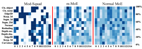
Figure 5: Visualization of the frequency that experts being selected for each task. We visualize the activation frequency of a MoE attention module in the 6-th transformer block with 15 experts and top-k as 6. The y-axis represents the tasks and the x-axis represents the 15 experts. We compare the visualization of Mod-Squad to m-MoE and normal MoE. All three methods have the exact same MoE module but with different MoE losses. Our frequency map is much sharp and sparse than other methods.

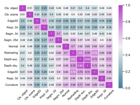
Figure 6: Task relation from Mod-Squad. We evaluate the similarity between tasks as the mean of the percentage of experts that they are sharing with the same input.

Task Relation. Mod-Squad can not only model the task relation implicitly like other multi-task models but also visualize it explicitly. We define the similarity between tasks as the mean of the percentage of experts that they are sharing given the same input. If two tasks are sharing more experts than other pairs of tasks, they are considered to be more related. This definition may not be perfectly accurate but is based on one simple rule: related tasks are more likely to share experts than unrelated tasks.

As shown in Fig. 6, Mod-Squad visualizes task relations in a correlation matrix with our new definition of task similarity. We notice that some of the structures among tasks are interesting: the 3D tasks including Normal, Reshading, two depth tasks, Edge3D, Keyp. 3D and curvature are grouped together; closed relation exists among two segmentations tasks and among two two depth tasks; Edge2D and Edge3D are not closed in the visualization. It demonstrates Mod-Squad can also be used as a visualization tool to explore the structure among tasks.

5 Conclusion

In this work, we propose Mod-Squad, a modular multi-task learner based on mixture-of-experts and a novel loss to address the gradient conflicts among tasks. We demonstrate its potential to scale up in both model capacity and target task numbers while keeping the computation cost low. It is noteworthy that Mod-Squad can be scaled down in model size with no performance drop for specific purposes. Future work could extend Mod-Squad to a large variety of tasks and scenes not only in the vision domain but also in other modalities (e.g., text and audio). We hope Mod-Squad will become an important building block of future efficient and modular foundation models.

Appendix

Table A1: Metric for more tasks on the taskonomy dataset. The experiment section in the paper demonstrates what metric we use for each task.

Model	Depth Zbu.						Edge2D	Keyp.3D	Segm. 2.5D
	$RMSE\downarrow$	Error $\downarrow$		$\delta$, within $\uparrow$			L1 dis. $\downarrow$	L1 dis. $\downarrow$	L1 dis. $\downarrow$
		Abs.	Rel.	1.25	$1.25^{2}$	$1.25^{3}$
STL	6.90	0.086	1.71	92.6	97.0	98.7	0.00500	0.072	0.155
MTL	6.75	0.083	1.30	93.1	96.8	98.9	0.00497	0.071	0.152
$M^{3}ViT$	6.73	0.081	1.30	93.4	97.3	98.9	0.00490	0.070	0.150
Mod-Squad	6.70	0.080	1.28	93.3	97.5	99.1	0.00482	0.068	0.147

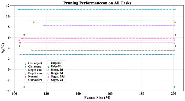
Figure A1: Visualization of the pruning results on each task. We set $\theta=0.1\%$ and do the pruning. Every tasks keep the same performance while reducing the parameters size from over 200M to lower than 120M.

A1 Metric for more task on the Taskonomy.

We provide more results with the task metric in Table. Appendix. Other tasks are shown in the paper already. Mod-Squad consistently have the best performance on these metrics.

A2 Pruning on different tasks.

We show the pruning results for all tasks on the Taskonomy in Figure. A2. We set $\theta=0.1\%$ and removing all experts have an activation frequency lower than $\theta$. Every tasks keep the same performance while reducing the parameters size from over 200M to lower than 120M. This demonstrate the effectiveness of Mod-Squad on all tasks.

A3 Ablation on Top-$K$.

As showin in Table. A2, we explore the effect on Top-$K$ for both MoE attention layer and MoE MLP layer. The experiment setting is the same as in Sec. A4. To control the FLOPs to be the same for different Top-$K$, the hidden dimension of attention experts and the mlp experts is divided by $K$. All experiments have the same parameter size and the same FLOPs.

A4 Ablation on number of experts.

As showin in Table. A3, we explore the effect on number of experts $E$ for both MoE attention layer and MoE MLP layer. For quick experiments, we use ViT-small as the backbone network. In default, we add MoE attention layer with 15 experts and Top-$K$ as 6 as well as MoE MLP layer with 16 experts and toop-k as 4. The MoE modules are added at every layer. We use $\Delta_{t}$ to evaluate the multi-task performance and report the parameters size. The $\Delta_{t}$ compare various version of models to the vanilla single task learning baseline with ViT-small. The experiments show that increasing experts number bring extra performance but the gain gradually diminish as the $E$ goes up. This conclusion hold true for both MoE attention layer and MoE MLP layer.

A5 More visualization on Mod-Squad.

We visualize Mod-Squad based on ViT-small as shown in Figure. A2 and Figure. A3. To better understand the relation between experts and task in all layers, we insert MoE attention layer and MoE MLP layer on every transformer block. In Figure. A2, the activation frequencies of MoE attention modules are shown in all transformer blocks with 15 experts and Top-$K$ as 6. In Figure. A3, the activation frequencies of MoE MLP modules are shown in all transformer blocks with 16 experts and Top-$K$ as 4. Both visualization demonstrates the sparsity of Mod-Squad in all layers for all tasks.

A6 Task relation from different layers of Mod-Squad.

In the paper, we define the similarity between tasks as the mean of the percentage of experts that they are sharing given the same input. We put all experts into the calculation of task similarity. However, we can also calculate the task similarity for each layer, by only put the experts from that specific layer into the calculation. As shown in Figure. A4, we visualize the task similarity for the first two layers, the middle two layers, and the last two layers of Mod-Squad. Mod-Squad is trained on the Taskonomy with ViT-base as the backbone and follow the same setting in our Taskonomy experiments in the paper. We notice that (1) all 3d tasks are very similar in the first layer; (2) all tasks are more similar to classification tasks in the middle two layers; (3) there is less similarity between tasks in the last two layers.

Table A2: Ablation study of Top-$K$ on MoE attention layer and MoE MLP layer.

	FLOPs(G)	Params(M)	Hidden Dim	$\Delta_{t}$
K=2	5.2	75	192	-0.4
K=4	5.2	75	96	1.3
K=6	5.2	75	64	3.5
K=9	5.2	75	42	3.1
K=12	5.2	75	32	2.2

(a) Ablation on Top-$K$ in the MoE attention layer.

	FLOPs(G)	Params(M)	Hidden Dim	$\Delta_{t}$
K=1	5.2	75	1536	3.3
K=2	5.2	75	768	3.3
K=4	5.2	75	384	3.5
K=6	5.2	75	256	3.2
K=8	5.2	75	192	3.1

(b) Ablation on Top-$K$ in the MoE MLP layer.

Table A3: Ablation study of expert number E on MoE attention layer and MoE MLP layer.

	Params(M)	$\Delta_{t}$
E=6	66	2.0
E=9	69	2.7
E=12	72	3.2
E=15	75	3.5
E=18	78	3.5

(a) Ablation on $E$ in the MoE attention layer.

	Params(M)	$\Delta_{t}$
E=4	33	2.2
E=8	47	2.7
E=12	61	3.3
E=16	75	3.5
E=20	90	3.5

(b) Ablation on E in the MoE MLP layer.

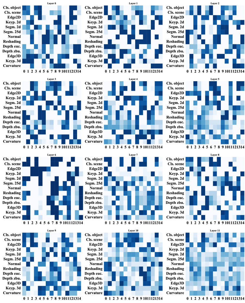
Figure A2: Visualization of the frequency that experts being selected for each task in the MoE attention layer. We visualize Mod-Squad based on ViT-small. The activation frequencies of MoE attention modules are shown in all transformer blocks with 15 experts and Top-$K$ as 6. The y-axis represents the tasks and the x-axis represents the experts. It demonstrates the sparsity of Mod-Squad in all layers for all tasks.

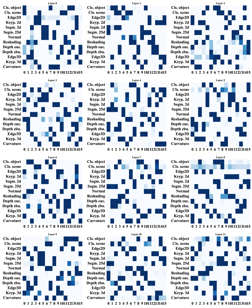
Figure A3: Visualization of the frequency that experts being selected for each task in the MoE MLP layer. We visualize Mod-Squad based on ViT-small. The activation frequencies of MoE MLP modules are shown in all transformer blocks with 16 experts and Top-$K$ as 4. The y-axis represents the tasks and the x-axis represents the experts. It demonstrates the sparsity of Mod-Squad in all layers for all tasks.

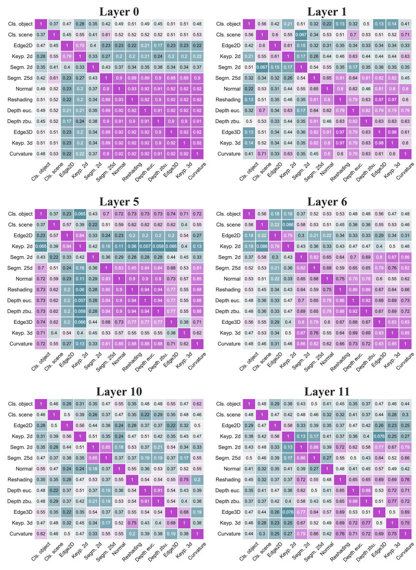
Figure A4: Visualization of task similarity from the first, the middle, and the last layers. For each layer $L_{i}$, we evaluate the similarity between a task pair as the mean of the percentage of experts in $L_{i}$ that task pairs are sharing with the same input.

References

- [1] Chanho Ahn, Eunwoo Kim, and Songhwai Oh. Deep elastic networks with model selection for multi-task learning. In Proceedings of the IEEE/CVF international conference on computer vision (ICCV), pages 6529–6538, 2019.
- [2] Felix JS Bragman, Ryutaro Tanno, Sebastien Ourselin, Daniel C Alexander, and Jorge Cardoso. Stochastic filter groups for multi-task cnns: Learning specialist and generalist convolution kernels. In Proceedings of the IEEE/CVF International Conference on Computer Vision (ICCV), pages 1385–1394, 2019.
- [3] Han Cai, Chuang Gan, Tianzhe Wang, Zhekai Zhang, and Song Han. Once for all: Train one network and specialize it for efficient deployment. In International Conference on Learning Representations (ICLR), 2020.
- [4] Rich Caruana. Multitask learning. Machine learning, 28(1):41–75, 1997.
- [5] Zhao Chen, Jiquan Ngiam, Yanping Huang, Thang Luong, Henrik Kretzschmar, Yuning Chai, and Dragomir Anguelov. Just pick a sign: Optimizing deep multitask models with gradient sign dropout. Advances in Neural Information Processing Systems, 33:2039–2050, 2020.
- [6] Alexey Dosovitskiy, Lucas Beyer, Alexander Kolesnikov, Dirk Weissenborn, Xiaohua Zhai, Thomas Unterthiner, Mostafa Dehghani, Matthias Minderer, Georg Heigold, Sylvain Gelly, Jakob Uszkoreit, and Neil Houlsby. An image is worth 16x16 words: Transformers for image recognition at scale. In International Conference on Learning Representations (ICLR), 2021.
- [7] David Eigen, Christian Puhrsch, and Rob Fergus. Depth map prediction from a single image using a multi-scale deep network. Advances in Neural Information Processing Systems (NeurIPS), 27, 2014.
- [8] William Fedus, Barret Zoph, and Noam Shazeer. Switch transformers: Scaling to trillion parameter models with simple and efficient sparsity. Journal of Machine Learning Research, 23(120):1–39, 2022.
- [9] Yuan Gao, Jiayi Ma, Mingbo Zhao, Wei Liu, and Alan L Yuille. Nddr-cnn: Layerwise feature fusing in multi-task cnns by neural discriminative dimensionality reduction. In Proceedings of the IEEE conference on computer vision and pattern recognition (CVPR), pages 3205–3214, 2019.
- [10] Song Han, Huizi Mao, and William J Dally. Deep compression: Compressing deep neural networks with pruning, trained quantization and huffman coding. International Conference on Learning Representations (ICLR), 2016.
- [11] Yang He, Guoliang Kang, Xuanyi Dong, Yanwei Fu, and Yi Yang. Soft filter pruning for accelerating deep convolutional neural networks. In International Joint Conference on Artificial Intelligence (IJCAI), pages 2234–2240, 2018.
- [12] Robert A Jacobs, Michael I Jordan, Steven J Nowlan, and Geoffrey E Hinton. Adaptive mixtures of local experts. Neural computation, 3(1):79–87, 1991.
- [13] Alex Kendall, Yarin Gal, and Roberto Cipolla. Multi-task learning using uncertainty to weigh losses for scene geometry and semantics. In Proceedings of the IEEE conference on computer vision and pattern recognition (CVPR), pages 7482–7491, 2018.
- [14] Iasonas Kokkinos. Ubernet: Training a universal convolutional neural network for low-, mid-, and high-level vision using diverse datasets and limited memory. In Proceedings of the IEEE conference on computer vision and pattern recognition (CVPR), pages 6129–6138, 2017.
- [15] Dmitry Lepikhin, HyoukJoong Lee, Yuanzhong Xu, Dehao Chen, Orhan Firat, Yanping Huang, Maxim Krikun, Noam Shazeer, and Zhifeng Chen. {GS}hard: Scaling giant models with conditional computation and automatic sharding. In International Conference on Learning Representations, 2021.
- [16] Mike Lewis, Shruti Bhosale, Tim Dettmers, Naman Goyal, and Luke Zettlemoyer. Base layers: Simplifying training of large, sparse models. In International Conference on Machine Learning (ICML), pages 6265–6274. PMLR, 2021.
- [17] Yawei Li, Shuhang Gu, Luc Van Gool, and Radu Timofte. Learning filter basis for convolutional neural network compression. In Proceedings of the IEEE International Conference on Computer Vision (ICCV), 2019.
- [18] Hanxue Liang, Zhiwen Fan, Rishov Sarkar, Ziyu Jiang, Tianlong Chen, Yu Cheng, Cong Hao, and Zhangyang Wang. Mvit: Mixture-of-experts vision transformer for efficient multi-task learning with model-accelerator co-design. In Advances in Neural Information Processing Systems (NeurIPS), December 2022.
- [19] Shikun Liu, Edward Johns, and Andrew J Davison. End-to-end multi-task learning with attention. In Proceedings of the IEEE conference on computer vision and pattern recognition (CVPR), pages 1871–1880, 2019.
- [20] Zhuang Liu, Mingjie Sun, Tinghui Zhou, Gao Huang, and Trevor Darrell. Rethinking the value of network pruning. In International Conference on Learning Representations (ICLR), 2019.
- [21] Ilya Loshchilov and Frank Hutter. Sgdr: Stochastic gradient descent with warm restarts. International Conference on Learning Representations (ICLR), 2017.
- [22] Ilya Loshchilov and Frank Hutter. Decoupled weight decay regularization. International Conference on Learning Representations (ICLR), 2019.
- [23] Kevis-Kokitsi Maninis, Ilija Radosavovic, and Iasonas Kokkinos. Attentive single-tasking of multiple tasks. In Proceedings of the IEEE conference on computer vision and pattern recognition (CVPR), pages 1851–1860, 2019.
- [24] Ishan Misra, Abhinav Shrivastava, Abhinav Gupta, and Martial Hebert. Cross-stitch networks for multi-task learning. In Proceedings of the IEEE conference on computer vision and pattern recognition (CVPR), pages 3994–4003, 2016.
- [25] Roozbeh Mottaghi, Xianjie Chen, Xiaobai Liu, Nam-Gyu Cho, Seong-Whan Lee, Sanja Fidler, Raquel Urtasun, and Alan Yuille. The role of context for object detection and semantic segmentation in the wild. In Proceedings of the IEEE conference on computer vision and pattern recognition (CVPR), pages 891–898, 2014.
- [26] Basil Mustafa, Carlos Riquelme, Joan Puigcerver, Rodolphe Jenatton, and Neil Houlsby. Multimodal contrastive learning with limoe: the language-image mixture of experts. arXiv preprint arXiv:2206.02770, 2022.
- [27] Xiaonan Nie, Shijie Cao, Xupeng Miao, Lingxiao Ma, Jilong Xue, Youshan Miao, Zichao Yang, Zhi Yang, and Bin Cui. Dense-to-sparse gate for mixture-of-experts. arXiv preprint arXiv:2112.14397, 2021.
- [28] Alex Renda, Jonathan Frankle, and Michael Carbin. Comparing rewinding and fine-tuning in neural network pruning. In International Conference on Learning Representations (ICLR), 2020.
- [29] Carlos Riquelme, Joan Puigcerver, Basil Mustafa, Maxim Neumann, Rodolphe Jenatton, André Susano Pinto, Daniel Keysers, and Neil Houlsby. Scaling vision with sparse mixture of experts. Advances in Neural Information Processing Systems (NeurIPS), 34:8583–8595, 2021.
- [30] Clemens Rosenbaum, Tim Klinger, and Matthew Riemer. Routing networks: Adaptive selection of non-linear functions for multi-task learning. In International Conference on Learning Representations (ICLR), 2018.
- [31] Noam Shazeer, *Azalia Mirhoseini, *Krzysztof Maziarz, Andy Davis, Quoc Le, Geoffrey Hinton, and Jeff Dean. Outrageously large neural networks: The sparsely-gated mixture-of-experts layer. In International Conference on Learning Representations, 2017.
- [32] Ximeng Sun, Rameswar Panda, Rogerio Feris, and Kate Saenko. Adashare: Learning what to share for efficient deep multi-task learning. Advances in Neural Information Processing Systems (NeurIPS), 33:8728–8740, 2020.
- [33] Yonglong Tian, Yue Wang, Dilip Krishnan, Joshua B Tenenbaum, and Phillip Isola. Rethinking few-shot image classification: a good embedding is all you need? In European Conference on Computer Vision (ECCV), pages 266–282. Springer, 2020.
- [34] Simon Vandenhende, Stamatios Georgoulis, Bert De Brabandere, and Luc Van Gool. Branched multi-task networks: deciding what layers to share. arXiv preprint arXiv:1904.02920, 2019.
- [35] Lemeng Wu, Mengchen Liu, Yinpeng Chen, Dongdong Chen, Xiyang Dai, and Lu Yuan. Residual mixture of experts. arXiv preprint arXiv:2204.09636, 2022.
- [36] Xiaogang Xu, Hengshuang Zhao, Vibhav Vineet, Ser-Nam Lim, and Antonio Torralba. Mtformer: Multi-task learning via transformer and cross-task reasoning. In Proceedings of the European Conference on Computer Vision (ECCV), 2022.
- [37] Jiahui Yu, Linjie Yang, Ning Xu, Jianchao Yang, and Thomas Huang. Slimmable neural networks. In International Conference on Learning Representations (ICLR), 2019.
- [38] Tianhe Yu, Saurabh Kumar, Abhishek Gupta, Sergey Levine, Karol Hausman, and Chelsea Finn. Gradient surgery for multi-task learning. Advances in Neural Information Processing Systems (NeurIPS), 33:5824–5836, 2020.
- [39] Amir R Zamir, Alexander Sax, William Shen, Leonidas J Guibas, Jitendra Malik, and Silvio Savarese. Taskonomy: Disentangling task transfer learning. In Proceedings of the IEEE conference on computer vision and pattern recognition (CVPR), pages 3712–3722, 2018.
- [40] Xiaofeng Zhang, Yikang Shen, Zeyu Huang, Jie Zhou, Wenge Rong, and Zhang Xiong. Mixture of attention heads: Selecting attention heads per token. Conference on Empirical Methods on Natural Language Processing (EMNLP), 2022.