Quadratic gravity potentials in de Sitter spacetime from Feynman diagrams

Abstract

We employ a manifestly covariant formalism to compute the tree-level amputated Green’s function of non-minimally coupled scalar fields in quadratic gravity in a de Sitter background. We study this Green’s function in the adiabatic limit, and construct the classical Newtonian potential. At short distances, the flat-spacetime Yukawa potential is reproduced, while the curvature gives rise to corrections to the potential at large distances. Beyond the Hubble radius, the potential vanishes identically, in agreement with the causal structure of de Sitter spacetime. For sub-Hubble distances, we investigate whether the modifications to the potential reproduce Modified Newtonian Dynamics.

1 Introduction

De Sitter spacetime plays a vital role in our current understanding of the Universe at different epochs. In early-time cosmology, de Sitter spacetime provides an accurate description of an inflationary universe, with evidence provided by the Cosmic Microwave Background (CMB) 2020 . Also at late cosmic times, observations of distant supernovae suggest an accelerated expansion of the universe, modeled by a de Sitter spacetime SupernovaCosmologyProject:1998vns ; SupernovaSearchTeam:1998fmf .

On the other hand, there are still significant open questions regarding de Sitter spacetime. First, we know that it arises in General Relativity (GR) as the solution to Einstein’s equation including a cosmological constant $\Lambda$. Usually attributed to so-called “dark energy” or an intrinsic “vacuum energy”, the origin of the cosmological constant, and its small present-day value of $67.66$ (km/s)/Mpc $=10^{-122}\;\ell_{\text{P}}^{2}$ Barrow:2011zp remains a mystery Martin:2012bt .

How to reconcile GR with quantum theory remains is currently unknown. In a flat background, perturbative quantization leads to a perturbatively non-renormalizable quantum theory tHooft:1974toh ; Goroff:1985sz ; Goroff:1985th . There are, by now, many ideas on how to resolve this, and construct a theory of Quantum Gravity. Of these approaches, string theory polchinski_1998 ; Tong:2009np , loop quantum gravity Rovelli:1997yv ; Dittrich:2004bn , and asymptotically safe quantum gravity (see for instance Wetterich:1992yh ; Reuter:1996cp ; Reuter:2019byg ; Percacci:2017fkn ; Eichhorn:2018yfc ; Pawlowski:2020qer ; Ferrero:2022hor for its continuum and Ambjorn:2012jv ; Loll:2019rdj for its discrete implementation) are notable examples. However, no candidate has been undisputedly successful so far.

Green’s functions in curved spacetime may provide insight into how to construct a consistent theory of quantum gravity. Being at the basis of observables in Quantum Field Theory, a proper understanding of scattering amplitudes in a gravitating background may help uncover how to incorporate long-distance curvature effects into quantum theory. Along another direction, by treating gravity as an effective field theory, scattering amplitudes involving loops introduce classical (post-Newtonian) corrections and quantum corrections to the gravitational potential Donoghue:1993eb ; Hamber:1995cq ; Bjerrum-Bohr:2002gqz ; Carrillo-Gonzalez:2021mqj ; Bjerrum-Bohr:2022blt ; Kosower:2022yvp .

Green’s functions in de Sitter spacetime are an important testing ground for such a program. Being the simplest non-trivially curved spacetime, amplitudes in de Sitter spacetime already exhibit the main challenges of quantizing in a generic curved spacetime, such as the absence of a unique invariant vacuum PhysRevD.32.3136 ; birrell_davies_1982 ; Mukhanov:2007zz ; Akhmedov:2019cfd , the obstructions in defining an $S$-matrix Witten:2001kn ; Bousso:2004tv ; Marolf:2012kh ; Mandal:2019bdu ; Giddings:2009gj ; deRham:2022hpx and the presence of singularities in correlation functions allen2 ; Allen1987THEGP ; Allen1987AnEO ; Floratos:1987ek ; PhysRevD.16.245 ; PhysRevD.45.2013 ; Akhmedov:2011pj ; Akhmedov:2013vka ; Akhmedov:2019esv ; Akhmedov:2020qxd ; Lochan:2018pzs ; Singh:2013dia ; Kim:2010cb ; Bros:1994dn ; Bros:1995js ; Bros:1998ik ; Higuchi:2010xt ; Higuchi:2002sc ; Fukuma:2013mx ; Arkani-Hamed:2015bza ; Arkani-Hamed:2018kmz ; Cacciatori:2007in .

Because of the absence of a unique invariant vacuum, the notion of scattering amplitude in curved spacetime is, in general, not well-defined and the construction is not free of ambiguities. On the other hand, the construction of well-defined Green’s functions in curved spacetime is possible, by picking a particular vacuum state and following the quantum field theoretical rules. We expect then that these objects encode physical information about particle scattering processes. As a guiding principle, one could aim to reproduce the flat spacetime result in the flat spacetime limit. This is the strategy adopted in this paper.

In Ferrero:2021lhd , we put forward a novel technique to compute Green’s functions in a de Sitter background. Key in this approach is the observation that Feynman diagrams can be represented by differential operators. In flat spacetime, these are commuting, so that we conveniently can go to momentum space. In curved spacetime, however, the non-commuting character of differential operators requires a more careful treatment.

The main result of Ferrero:2021lhd was the tree-level amplitude amputated Green’s function of the gravity-mediated scattering of two minimally coupled massive scalars in de Sitter spacetime. Here the gravitational dynamics is specified by the Einstein-Hilbert action. Employing an expansion around infinite scalar masses, we use this amplitude to compute the de Sitter spacetime generalization of the Newtonian potential. Remarkable features of this potential are curvature-dependent corrections corresponding to a repulsive force, consistent with the picture of de Sitter spacetime as an expanding universe, and a vanishing potential at super-Hubble distances, encoding a causal separation by the de Sitter horizon.

In this paper, we extend this computation to quadratic gravity (QuadG) Sexl ; Havas ; Donoghue:2021cza ; Salvio:2019ewf . In the pure-gravity sector, we include all terms in the action up to four derivatives of the metric, while we also allow for a non-minimal $R\phi\phi$-coupling between the scalar fields and the Ricci scalar.

The extension to QuadG is interesting for a number of reasons. First, QuadG successfully provides the dynamics of primordial graviton fluctuations Starobinsky:1980te ; Ketov:2012jt . Its predictions for inflationary power spectra and spectral indices are in excellent agreement with observational data Koshelev:2017tvv ; Koshelev:2020foq , and lead to constraints on the gravitational couplings Vilenkin:1985md ; Berry:2011pb ; Cembranos:2008gj ; Kapner:2006si .

Second, QuadG is attractive from a theoretical perspective. As was shown by Stelle Stelle:1976gc ; Stelle:1977ry it is perturbatively renormalizable in flat spacetime, in contrast to Einstein-Hilbert gravity. However, this does not come for free. The addition of four-derivative terms in the action implies that the resulting Hamiltonian is unbounded from below. Classically, this leads to the Ostrogradsky instability Ostrogradsky . At the quantum level, it is signaled by the appearance of a massive spin-2 ghost Antoniadis ; Tomboulis:1977jk ; Donoghue_ghost .

Third, as we demonstrated in Ferrero:2021lhd , the Newtonian potential receives corrections due to the background curvature. In GR, these corrections are suppressed by the inverse de Sitter radius. Therefore, the potential meets all observational tests on length scales ranging from table-top to solar system Sokolowski:2008kf ; Capozziello:2009ss ; Naf:2010zy ; Conroy:2014eja ; Alvarez-Gaume:2015rwa ; Edholm:2016hbt ; Cheung:2018wkq . In QuadG, however, the new coupling constants induce additional length scales, leading possibly to corrections to the potential at much smaller lengths. Thus, the computation of the Newtonian potential in QuadG may lead to additional constraints on the non-minimal couplings.

Replacing the classical Newtonian potential by a more general potential falls into the class of Modified Newtonian Dynamics Milgrom1983AMO ; Milgrom:2011kx ; Famaey:2011kh ; deAlmeida:2018kwq . This has been used to successfully account for the observed properties of rotation curves of galaxies Brouwer:2021nsr ; mond1 ; Blanchet:2011pv . Therefore, it is seen as an alternative to the dark matter (DM) hypothesis. In our setting, we will test whether the modifications to the Newtonian potential due to QuadG in de Sitter spacetime give rise to a DM-like MOND scenario.

This paper is organized as follows. In Section 2 we derive the Yukawa potential and discuss the analogous construction of the gravitational potential. In Section 3, we describe how to compute the Green’s function of a two-to-two scalar process in a de Sitter background in QuadG. In Section 4, we compute the adiabatic expansion of this Green’s function. This is translated to the nonrelativistic potential in Section 5. We end with a brief summary and concluding remarks in Section 6. We collect our conventions for de Sitter spacetime in Appendix A. Details regarding the adiabatic expansion in general and the Green’s function are relegated to Appendix B and Appendix C, respectively.

2 Warmup: the Yukawa potential

Before constructing the Green’s function of a graviton-mediated scalar-to-scalar process, we will set the stage by following the standard derivation of the the Yukawa potential for a massive $\phi^{3}$-scalar theory scalar-to-scalar scattering process in flat spacetime.

The Yukawa potential can be derived as the lowest order amplitude of the interaction of a pair of scalars. The Yukawa interaction couples them to another exchanged scalar field with the interaction term $g\;\phi^{3}$. The action of the three scalars then reads

$$S_{\text{}}=\int\text{d}^{d}x\;\left(\frac{1}{2}\partial_{\mu}\phi\partial^{\mu}\phi+\frac{1}{2}\partial_{\mu}\chi\partial^{\mu}\chi-\frac{m^{2}}{2}\phi^{2}-\frac{M^{2}}{2}\chi^{2}-g\;\phi^{2}\chi\right)\,\text{.}$$ (1)

Figure 1: Tree-level scalar-to-scalar $\phi^{2}$-scattering amplitude for the process $\phi_{1}\phi_{2}\to\phi_{3}\phi_{4}$ ($t$-channel). Time flows from the left to the right.

The scattering amplitude for two scalars, one with initial momentum $p_{1}$ and the other with momentum $p_{2}$, exchanging a scalar $\chi$ with momentum $k$ (see Figure 1), is constructed by applying the Feynman rules:

1. For each vertex associate a factor of $g$ with the amplitude; since this diagram has two vertices, the total amplitude will have a factor of $g^{2}$;

2. The Feynman rule for a particle exchange is to use the propagator; the propagator for a scalar with mass $M$ is $-\frac{4\pi}{k^{2}+M^{2}}$;

3. Thus, we see that the Feynman amplitude for this interaction is nothing more than

   $$\tilde{V}(k)=-g^{2}\frac{4\pi}{k^{2}+M^{2}}\stackrel{{\scriptstyle M\gg|\vec{k}|}}{{=}}-g^{2}\frac{4\pi}{|\vec{k}|^{2}+M^{2}}$$ (2)

   where in the last equality we have applied the so-called Born approximation: we assumed that the mass is much greater than the exchanged 3-momentum.

This is seen to be the Fourier transform of the Yukawa potential by examining its Fourier transform:

$$V(r)=\frac{g^{2}}{(2\pi)^{3}}\int e^{\mathrm{i}\vec{k}\cdot\vec{r}}\frac{4\pi}{|\vec{k}|^{2}+M^{2}}\text{d}^{3}\vec{k}=-g^{2}\;\frac{e^{-M\;r}}{r}\,\text{.}$$ (3)

The potential is monotonically increasing in $r$ and it is negative, implying that the force is attractive.

2.1 Gravitational potential around flat spacetime

In the following subsection we will extend this computation to gravitational interactions Bjerrum-Bohr:2002gqz by sketching the derivation of the Newtonian potential, and to the Quadratic Gravity action. Here, both cases are treated in flat spacetime.

Ref. Bjerrum-Bohr:2002gqz sketched how the Newtonian $1/r$-potential could be derived by performing the Born approximation to the following scattering process: they considered a two-to-two-scalars graviton mediated scattering amplitude. Due to the masslessness of the exchanged graviton, this resulted in a $1/r$ interaction potential.

Analogously, by studying the propagating modes corresponding to Quadratic Gravity around flat spacetime, the same Yukawa terms should arise Alvarez-Gaume:2015rwa . Consider the four-derivative gravitational action (in the metric $\hat{g}_{\mu\nu}$) in 4 dimensions and two non-minimally coupled scalar fields

$$S[\hat{g},\phi,\chi]=\frac{1}{16\pi G_{N}}\int\differential[d]{x}\sqrt{-\hat{g}}\,\bigg{(}\begin{aligned} &-2\Lambda+\hat{R}+\frac{\alpha_{R}}{6}\hat{R}^{2}-\frac{\alpha_{C}}{2}\hat{C}_{\mu\nu\rho\sigma}\hat{C}^{\mu\nu\rho\sigma}\\ &-\frac{1}{2}\phi\left(\hat{\square}+m^{2}_{\phi}+\alpha_{\phi}\hat{R}\right)\phi-\frac{1}{2}\chi\left(\hat{\square}+m^{2}_{\chi}+\alpha_{\chi}\hat{R}\right)\chi\bigg{)}\,\text{.}\end{aligned}$$ (4)

The flat-spacetime amplitude of a $\phi\chi\to\phi\chi$ graviton-mediated scattering amplitude (see Figure 2) can be computed applying the recipe of the previous subsection. By expanding quadratically the action around Minkowski space $\hat{g}_{\mu\nu}=\eta_{\mu\nu}+h_{\mu\nu}$ and choosing the de Donder gauge fixing one can derive the different contributions for the propagators. They can be interpreted as the propagator of a massless spin-0 and spin-2 particle (the graviton) and a spin-0 particle with mass parameter $M^{2}=\alpha_{R}^{-1}$ and a spin-2 particle with mass $M^{2}=\alpha_{C}^{-1}$. These appear in the amplitude with suitable prefactors and signs. Schematically, denoting $q$ the momentum of the exchanged particle, the different contributions to the propagators are:

spin-2: $$\frac{1}{q^{2}},\qquad\frac{1}{q^{2}+\alpha_{C}^{-1}}$$ (5)

spin-0: $$\frac{1}{q^{2}},\qquad\frac{1}{q^{2}+\alpha_{R}^{-1}}$$ (6)

The related potential can be obtained by performing the Fourier transform of the amplitude. We obtain

$$\ V_{\text{Mink}}(r)\propto G_{N}\left(-\frac{1}{r}-\frac{1}{3}\frac{1}{r}\mathrm{e}^{-r/\sqrt{\alpha_{R}}}+\frac{4}{3}\frac{1}{r}\mathrm{e}^{-r/\sqrt{\alpha_{C}}}\right)\;.$$ (7)

The first term represents the Newtonian contribution, while the other two terms are Yukawa potentials due to the presence of quadratic interactions.

It is important to emphasize, that the two additional Yukawa contributions appear with two opposite signs. The $\alpha_{C}$ term has a positive sign, meaning that it competes with the Newtonian contribution and is repulsive. Demanding that the potential should reproduce the Newtonian behavior at short distances will impose constraints on the value of $\alpha_{C}$.

3 The quadratic gravity Green’s function in de Sitter spacetime

In this section, we compute the Green’s function of a two-to-two particle scattering process in de Sitter spacetime. We consider the graviton-mediated scattering of two scalars $\phi$ and $\chi$, in the process $\phi\chi\to\phi\chi$. At tree level, this process is described by the $t$-channel Feynman diagram, depicted in Figure 2. Here we generalize this Feynman diagram to de Sitter spacetime.

We first give a heuristic interpretation of Green’s functions in curved spacetime in Section 3.1. We then set the stage by specifying the action in Section 3.2. We provide details on how to compute the Green’s function in de Sitter spacetime in Section 3.3. The resulting amputated Green’s function is then presented in Section 3.4. We finish this section with a few remarks in Section 3.5.

Figure 2: Feynman diagram of the scattering process $\phi\chi\to\phi\chi$ mediated by a graviton $h_{\mu\nu}$.

3.1 Gedankenexperiment

In this section, we will briefly discuss the interpretation of scattering processes from an experimental point of view. Scattering amplitudes represent a technical tool developed with the purpose to connect QFT and collider experiments. However, as previously mentioned, due to the lack of a description of an $S$-matrix in QFT in curved spacetime, the generalization to possible collision experiments in general spacetimes has not been performed yet.

By constructing Green’s functions in de Sitter spacetime in a fully covariant way, we can mimic the connection to experiments generally used in Minkowski spacetime. In this way we circumvent the lack of $S$-matrix elements in de Sitter. For the sake of simplicity, here we will restrict the discussion to GR interactions, considering in the gravitational action only the Einstein–Hilbert term (neglecting higher curvature interactions).

The resulting picture is the following: we prepare two heavy-mass particles in a de Sitter space and localize them in space. The two particles scatter. Once the process has finished, we detect where the outgoing particles have ended up.

In particular we will work in the expanding Poincaré patch. Here the particles will be Bunch–Davies waves, i.e., the wave functions solve the wave equation in the expanding Poincaré patch. The Bunch–Davies vacuum is a state that has no positive energy excitations at the past infinity of the expanding Poincaré patch. In fact near the boundary we can define what we mean by particle and what we mean by positive energy, because every momentum experiences infinite blue shift towards the past of the patch. Here, high energy harmonics are not sensitive to the comparatively small curvature of the background space and behave as if they are in flat space.

Due to the spatial homogeneity of the conformally flat patch and also of the initial states that we consider, it will be natural to perform the Fourier transformation along the spatial directions. The explicit computation of the Green’s function will allow us to pass from momentum space to position space and to construct the potential.

3.2 Action

We start our computation by introducing the action $S$. We use an action that is a functional of the (dynamical) spacetime metric $\hat{g}$ and two scalar fields $\phi$ and $\chi$. In order to consistently handle the gauge degrees of freedom in the metric fluctuations, we employ the background field method, depending on the background metric $\bar{g}$. We denote quantities defined with respect to the dynamical metric $\hat{g}$ by a hat, while objects defined using the background metric $\bar{g}$ are denoted by a bar. The action is then of the following form:

$$S=S_{\text{grav}}[\hat{g}]+S_{\text{gf}}[\hat{g};\bar{g}]+S_{\text{sc}}[\phi,\hat{g}]+S_{\text{sc}}[\chi,\hat{g}]\,\text{.}$$ (8)

Let us now explicitly formulate each contribution to the action. For the gravitational interaction $S_{\text{grav}}$, we take the four-derivative action

$$S_{\text{grav}}[\hat{g}]=\frac{1}{16\pi G_{N}}\int\differential[d]{x}\sqrt{-\hat{g}}\,\bigg{(}\begin{aligned} &-2\Lambda+\hat{R}+\alpha_{R}\frac{d-2}{4(d-1)}\hat{R}^{2}\\ &-\alpha_{C}\frac{d-2}{4(d-3)}\hat{C}_{\mu\nu\rho\sigma}\hat{C}^{\mu\nu\rho\sigma}+\frac{1}{2(d-3)(d-4)}\alpha_{E}E_{4}\bigg{)}\,\text{.}\end{aligned}$$ (9)

For the time being, no specification of the sign of the cosmological constant $\Lambda$ is required.

In (9), $E_{4}$ is the Euler density in four dimensions:

$$E_{4}=\hat{R}^{2}-4\hat{R}_{\mu\nu}\hat{R}^{\mu\nu}+\hat{R}_{\alpha\beta\gamma\delta}\hat{R}^{\alpha\beta\gamma\delta}\,\text{.}$$ (10)

For $d=4$, the integral over $E_{4}$ is a topological invariant. Thus, for this dimension we set $\alpha_{E}$ to zero, since it will not contribute to any dynamical quantity. In a similar fashion, the $C^{2}$ and $R^{2}$ are non-dynamical for $d\leq 3$ and $d\leq 2$ dimensions, respectively. We therefore set the $\alpha_{C}$ and $\alpha_{R}$ couplings to zero in these dimensions, too. In flat spacetime, the $\alpha_{R}$ and $\alpha_{C}$ couplings induce massive spin-0 and spin-2 poles in the graviton propagator. We have chosen the normalization in such a way that in flat spacetime, $\alpha_{R}$ denotes the inverse mass of the spin-0 pole, while $\alpha_{C}$ denotes the inverse mass of the spin-2 pole Stelle:1976gc .

Next, we specify in (8) a de Donder type gauge fixing action, necessary to obtain a well-defined graviton propagator:

$$S_{\text{gf}}[\hat{g};\bar{g}]=-\frac{1}{16\pi G_{N}}\frac{1}{2\alpha_{\text{gf}}}\int\differential[d]{x}\sqrt{-\bar{g}}\,\bar{g}^{\mu\nu}\mathcal{F}_{\mu}[\hat{g},\bar{g}]\mathcal{F}_{\nu}[\hat{g},\bar{g}]\,\text{,}$$ (11)

where the gauge fixing operator is defined as

$$\mathcal{F}_{\mu}[\hat{g},\bar{g}]=\delta_{\mu}^{\beta}\bar{g}^{\rho\sigma}\bar{\nabla}_{\rho}\hat{g}_{\sigma\beta}-\frac{1+\beta_{\text{gf}}}{d}\bar{g}^{\alpha\beta}\bar{\nabla}_{\mu}\hat{g}_{\alpha\beta}\,\text{.}$$ (12)

Here the gauge fixing parameters $\alpha_{\text{gf}}$ and $\beta_{\text{gf}}$ generalize the de Donder gauge, and allow to track gauge dependence explicitly. The Faddeev-Popov ghosts will not contribute to the Green’s function, for the reason that they do not couple to the scalar fields. The specific form of their action is therefore not needed for our purposes.

Finally, the matter sector is given by non-minimally coupled massive scalar fields $\phi$ and $\chi$, whose action takes the form

$$S_{\text{sc}}[\phi,\hat{g}]=-\frac{1}{2}\int\differential[d]{x}\sqrt{-\hat{g}}\,\phi\left(\hat{\square}+m_{\phi}^{2}+\alpha_{\phi}\hat{R}\right)\phi\,\text{.}$$ (13)

Here we have expressed the covariant d’Alembertian by $\hat{\square}=-\hat{g}^{\mu\nu}\hat{\nabla}_{\mu}\hat{\nabla}_{\nu}$.

3.3 Computation of the Green’s functional

We will now give a brief description of how to compute the Feynman diagram in a curved background geometry. We follow the computation from Ferrero:2021lhd ; we refer to this paper for additional details.

The tree-level Green’s function associated to the diagram in Figure 2 is obtained by contracting the graviton-scalar-scalar 3-point vertices with the graviton propagator. These are computed by taking functional derivatives of the action $S$ with respect to the fields, and projecting onto a solution to the equation of motion. For the scalar fields, the equation of motion is given by the (non-minimal) Klein-Gordon equation:

$$\hat{\square}\phi=-(m_{\phi}^{2}+\alpha_{\phi}\hat{R})\phi\,\text{,} \hat{\square}\chi=-(m_{\chi}^{2}+\alpha_{\chi}\hat{R})\chi\,\text{.}$$ (14)

We observe that $\phi=\chi=0$ is a solution to the equation of motion. The equation of motion for the metric is that of QuadG. We will look for de Sitter solutions, which means that the constant Ricci scalar is the only nonzero curvature tensor. The Ricci scalar $R$ is then given by the quadratic equation

$$R=\frac{2d}{d-2}\Lambda-\frac{d-4}{4(d-1)}\alpha_{R}R^{2}\,\text{.}$$ (15)

We write

$$\hat{g}_{\mu\nu}=\bar{g}_{\mu\nu}+h_{\mu\nu}\,\text{,}$$ (16)

where $\bar{g}_{\mu\nu}$ is a de Sitter metric whose Ricci scalar $\bar{R}$ satisfies (15). Functional derivatives with respect to $\hat{g}$ are then conveniently computed by expanding around $\bar{g}_{\mu\nu}$.

By taking one functional derivative with respect to the metric and two with respect to the scalar fields, we obtain the three-point vertices. Subsequently, we set all fields to their background values. Thus, we define

$$\mathcal{T}^{(h\phi\phi)}=\evaluated{\frac{\delta^{3}S}{\delta h\delta\phi\delta\phi}}_{\begin{subarray}{c}\hat{g}=\bar{g}\\ \phi=\chi=0\end{subarray}}\,\text{,} \mathcal{T}^{(h\chi\chi)}=\evaluated{\frac{\delta^{3}S}{\delta h\delta\chi\delta\chi}}_{\begin{subarray}{c}\hat{g}=\bar{g}\\ \phi=\chi=0\end{subarray}}\,\text{.}$$ (17)

The graviton propagator is given by the inverse of the two-point function:

$$\mathcal{G}^{(hh)}=\evaluated{\left[\frac{\delta^{2}S}{\delta h\delta h}\right]^{-1}}_{\begin{subarray}{c}\hat{g}=\bar{g}\\ \phi=\chi=0\end{subarray}}\,\text{.}$$ (18)

Note that in order to make the inversion well-defined, it was necessary to include the gauge fixing action $S_{\text{gf}}$ in (8).

The tree-level Green’s function associated to the diagram in Figure 2 is now obtained by contracting the three-point vertices with the graviton propagator. Rather than treating the Green’s function as a multilinear operator acting on fields, it is convenient to contract the Green’s function with four test fields:

$$\mathcal{A}[\chi_{1},\chi_{2},\phi_{1},\phi_{2}]=\int\differential[d]{x}\sqrt{-\bar{g}}\,\left[\mathcal{T}^{(h\chi\chi)}\left(\chi_{1},\chi_{2}\right)\right]^{\mu\nu}\tensor{\left[\mathcal{G}^{(hh)}\right]}{{}_{\mu\nu}^{\rho\sigma}}\left[\mathcal{T}^{(h\phi\phi)}\left(\phi_{1},\phi_{2}\right)\right]_{\rho\sigma}\,\text{.}$$ (19)

Here the $\mathcal{T}^{(h\chi\chi)}(\chi_{1},\chi_{2})$ denotes the three-point vertex (17) acting on two test fields $\chi_{1}$ and $\chi_{2}$. The object $\mathcal{A}$ will be referred to as Green’s functional. Since (19) only contains objects in the de Sitter background, to simplify the notation, we will omit the bar to denote the background metric and its derived objects.

At this point, we note that the building blocks of (19) are noncommuting linear differential operators acting on the scalar fields and metric fluctuations. This can be contrasted to two common methods used to compute Feynman diagrams. First of all, in flat spacetime, one has access to momentum-space techniques to easily convert the vertices and propagators to a number. In curved spacetime, derivatives do not commute and a description in terms of Fourier transforms does not exist, in general. Hence, noncommuting differential operators are the natural generalization of flat-spacetime momenta. Second, considering vertices and propagators as operators greatly simplifies composition and contraction of Feynman diagram elements. The differential operator language has the advantage over computations using position-space integral kernels like Green’s functions, which would imply performing lengthy integrals over de Sitter spacetime.

We computed the Green’s functional (19) using the Mathematica tensor algebra package xAct Brizuela:2008ra ; DBLP:journals/corr/abs-0803-0862 ; Nutma:2013zea ; xActwebpage . We used the procedure outlined in Ferrero:2021lhd to construct the graviton propagator and to sort and contract the covariant derivatives.

The Green’s functional (19) consists of covariant derivatives acting on the scalar fields, and scalar curvatures. The Green’s function can be simplified using the on-shell conditions (14), integration by parts and the commutation techniques developed in Knorr:2020bjm ; Ferrero:2021lhd . These methods can be used to bring the Green’s functional to a standard form. We will require that the Green’s functional is manifestly symmetric in the external fields. Since the vertices contain at most two uncontracted derivatives, we infer that the Green’s function can be built using a scalar vertex structure, and a symmetric rank-two tensor vertex structure. For the scalar vertex, it is convenient to define

$$V[\phi_{1},\phi_{2}]=\left[m_{\phi}^{2}+(d-1)\left(\alpha_{\phi}-\frac{d-2}{4(d-1)}\right)\square\right]\phi_{1}\phi_{2}\,\text{,}$$ (20)

where the d’Alembertian acts on the product $\phi_{1}\phi_{2}$. For the tensor vertex we choose

$$T_{\mu\nu}[\phi_{1},\phi_{2}]=(\nabla_{(\mu}\phi_{1})(\nabla_{\nu)}\phi_{2})-\frac{1}{d}g_{\mu\nu}(\nabla_{\gamma}\phi_{1})(\nabla^{\gamma}\phi_{2})-\alpha_{\phi}\left[\nabla_{\mu}\nabla_{\nu}+\frac{1}{d}g_{\mu\nu}\square\right]\phi_{1}\phi_{2}\,\text{.}$$ (21)

Finally, it will be convenient to define the operators

$$\mathcal{G}_{r}(\square;\zeta)=\Big{(}\square+\big{(}r(r+d-2)+\zeta\big{)}H^{2}\Big{)}^{-1}\,\text{.}$$ (22)

Here we define the Hubble parameter by $H^{2}=\frac{R}{d(d-1)}$, following the conventions from Appendix A. We will refer to the operator $\mathcal{G}_{r}(\square;\zeta)$ as propagator. The label $r$ denotes the rank of the tensor it acts upon. We will refer to the dimensionless number $\zeta$ as the mass parameter; using slightly sloppy terminology, it parameterizes the graviton mass and can be related to the unitary irreducible representations of the graviton degrees of freedom Garidi:2003ys ; Pejhan:2018ofn ; Joung:2006gj ; Joung:2007je ; Sengor:2019mbz ; Gazeau:2006gq .

3.4 Result

We will now present the resulting Green’s functional. This constitutes the first major result of this paper. The Green’s functional (19) is given by

$$\mathcal{A}=16\pi G_{N}\,c(\alpha_{R},\alpha_{E})\bigg{[} -\frac{\zeta_{C}+d}{\zeta_{C}-\zeta_{h}}\Big{(}\mathcal{A}_{2}(\zeta_{h})-\mathcal{A}_{2}(\zeta_{C})\Big{)}$$ (23)

$$+\frac{1}{d(d-1)}\frac{\zeta_{C}}{\zeta_{C}-\zeta_{h}}\Big{(}\mathcal{A}_{0}(\zeta_{h})-\mathcal{A}_{0}(\zeta_{C})\Big{)}$$

$$+\frac{1}{(d-1)(d-2)}\Big{(}\mathcal{A}_{0}(\zeta_{h})-\mathcal{A}_{0}(\zeta_{R})\Big{)}\bigg{]}\,\text{.}$$

Here we have defined the partial Green’s functionals

$$\mathcal{A}_{0}(\zeta) =\int\differential[d]{x}\sqrt{-g}\,V[\chi_{1},\chi_{2}]\,\mathcal{G}_{0}(\square;\zeta)\,V[\phi_{1},\phi_{2}]\,\text{,}$$ (24)

$$\mathcal{A}_{2}(\zeta) =\int\differential[d]{x}\sqrt{-g}\,T_{\alpha\beta}[\chi_{1},\chi_{2}]\,\mathcal{G}_{2}(\square;\zeta)\,T^{\alpha\beta}[\phi_{1},\phi_{2}]\,\text{,}$$ (25)

the dimensionless mass parameters

$$\zeta_{R} =\frac{1}{\alpha_{R}H^{2}}+\frac{1}{2}d(d-4)+\frac{\alpha_{E}}{\alpha_{R}}\,\text{,} \zeta_{h}=-2(d-1)\,\text{,}$$ (26)

$$\zeta_{C} =\frac{1}{\alpha_{C}H^{2}}-d+\frac{1}{2}d(d-2)\frac{\alpha_{R}}{\alpha_{C}}+\frac{\alpha_{E}}{\alpha_{C}}\,\text{.}$$

and the coefficient

$$c(\alpha_{R},\alpha_{E})=\frac{1}{1+\alpha_{E}H^{2}}\frac{\zeta_{R}-\frac{1}{2}d(d-4)}{\zeta_{R}+d}\,\text{.}$$ (27)

3.5 Discussion

From the Green’s functional (23), the following observations can be made straightaway.

First, we note that the Green’s function does not depend on the gauge parameters $\alpha_{\text{gf}}$ and $\beta_{\text{gf}}$. This shows that the on-shell Green’s function is gauge fixing independent, conform the expectation that the Green’s function (and hence its related scattering amplitude) is related to an observable.

Second, we note that the scalar vertex $V[\phi_{1},\phi_{2}]$ vanishes for a conformally coupled scalar field $m_{\phi}=0$, $\alpha_{\phi}=\frac{d-2}{4(d-1)}$. This greatly simplifies the Green’s function. For this reason, the conformally coupled scalar field has been studied widely Tsamis:1992xa ; Park:2015kua ; Frob:2016fcr ; Frob:2017smg ; Glavan:2020ccz .

Third, we observe that the Green’s functional (23) depends on three mass parameters $\zeta_{h}$, $\zeta_{R}$ and $\zeta_{C}$. In the limit $H\to 0$, these correspond to masses of zero, $\alpha_{R}^{-1}$ and $\alpha_{C}^{-1}$, respectively. Hence, these mass parameters correspond to the massless graviton, and the spin-0 and spin-2 mass poles. At first inspection, the negative value of $\zeta_{h}$ may seem to yield a tachyonic particle. However, it is important to keep in mind that due to the nonzero curvature the correspondence between the sign of the mass and the causal behavior is not obvious Garidi:2003ys ; Pejhan:2018ofn .

Fourth, it is now relatively simple to obtain the Green’s functions of GR, $R^{2}$-gravity and $C^{2}$-gravity from this expression, by taking the following limits:

GR: $$\qquad\alpha_{C}\to 0,\alpha_{R}\to 0\,\text{;}$$ (28)

$$R^{2} \qquad\alpha_{C}\to 0\,\text{;}$$-gravity: (29)

$$C^{2} \qquad\alpha_{R}\to 0\,\text{.}$$-gravity: (30)

Furthermore, we obtain the Green’s function in Minkowski spacetime by taking the limit

$$\text{Minkowski spacetime:}\qquad H\to 0\,\text{.}$$ (31)

Let us first consider the latter limit. We note that the mass parameters $\zeta_{C}$ and $\zeta_{R}$ go to infinity; we then find the following limits for the coefficients:

$$\lim_{H\to 0}c(\alpha_{R},\alpha_{E})=\lim_{H\to 0}\frac{\zeta_{C}+d}{\zeta_{C}-\zeta_{h}}=\lim_{H\to 0}\frac{\zeta_{C}}{\zeta_{C}-\zeta_{h}}=1\,\text{.}$$ (32)

The propagators reduce to

$$\lim_{H\to 0}\mathcal{G}_{0}(\square;\zeta_{h}) =\lim_{H\to 0}\mathcal{G}_{2}(\square;\zeta_{h})=\square^{-1}\,\text{,}$$ (33)

$$\lim_{H\to 0}\mathcal{G}_{0}(\square;\zeta_{C}) =\lim_{H\to 0}\mathcal{G}_{2}(\square;\zeta_{C})=\Big{(}\square+\alpha_{C}^{-1}\Big{)}^{-1}\,\text{,}$$

$$\lim_{H\to 0}\mathcal{G}_{0}(\square;\zeta_{R}) =\Big{(}\square+\alpha_{R}^{-1}\Big{)}^{-1}\,\text{.}$$

This is consistent with the amplitude found in Stelle:1976gc ; Donoghue:1994dn . Inspecting the propagators (33), we see that the Minkowski spacetime amplitude corresponds to a massless spin-0 and spin-2 particle, corresponding to the graviton, and in addition a massive spin-0 particle of mass $\alpha_{R}^{-1}$ and a massive spin-2 particle of mass $\alpha_{C}^{-1}$ Stelle:1976gc ; Stelle:1977ry .

In a similar fashion, we consider $R^{2}$- and $C^{2}$-gravity. Taking the limit $\alpha_{R}\to 0$ and $\alpha_{C}\to 0$, we find that $\zeta_{R}$ and $\zeta_{C}$ are linearly divergent, respectively. Hence, provided that the coefficients of the propagators remain finite, we conclude that the propagators $\mathcal{G}_{0}(\square;\zeta_{C})$ and $\mathcal{G}_{2}(\square;\zeta_{C})$ are suppressed in $R^{2}$-gravity, corresponding to a decoupling of the spin-2 Stelle particle, while in $C^{2}$-gravity the propagator $\mathcal{G}_{0}(\square;\zeta_{R})$ is suppressed, corresponding of a decoupling of the spin-0 massive particle from the theory. It remains to check that the coefficients of the propagator stay finite; we compute

$$\lim_{\alpha_{R}\to 0}c(\alpha_{R},\alpha_{E})=\frac{1}{1+\alpha_{E}H^{2}}\,\text{,} \lim_{\alpha_{C}\to 0}\frac{\zeta_{C}+d}{\zeta_{C}-\zeta_{h}}=\lim_{\alpha_{C}\to 0}\frac{\zeta_{C}}{\zeta_{C}-\zeta_{h}}=1\,\text{.}$$ (34)

This justifies the assertion that the massive particles decouple in $R^{2}$- and $C^{2}$-gravity.

4 The Green’s function in the adiabatic limit

We will now inspect the Green’s functional in more detail. Since the Green’s functional is given by abstract differential operators on de Sitter spacetime, it is not easy to draw conclusions about its physical properties. Therefore, we resort to expansion methods to turn (23) into a concrete numerical expression. We employ an expansion around the scalar masses $\mu=m/H=\infty$, following Ferrero:2021lhd . This is a specific realization of the so-called adiabatic expansion Agullo:2014ica ; Moreno-Pulido:2022phq ; Junker:2001gx ; Lueders:1990np ; Olbermann:2007gn ; Fulling1979RemarksOP ; Fulling:1974zr ; Fulling:1989nb ; Parker:1968mv ; Parker:1969au ; Parker:1971pt ; Parker:1974qw ; Parker:2009uva ; Birrell_adiabatic ; Bunch_adiabatic ; Bunch:1978aq ; Haro:2008zz ; Winitzki:2005rw ; Zeldovich1 ; Zeldovich2 . This can be understood from the observation that an expansion around $\mu=\infty$ implies that the evolution of de Sitter spacetime is much slower than the Compton frequency of the scalar fields.

In Section 4.1, we describe the algorithm used to compute the adiabatic limit of the Green’s functional. This computation was pioneered in the context of GR in Ferrero:2021lhd ; here we generalize the calculation to QuadG. The properties of the resulting Green’s function are studied in Section 4.2. In Appendix B, we collect several details regarding the adiabatic limit obtained in Ferrero:2021lhd . Appendix C is devoted to the numerical techniques to obtain the Green’s function in the adiabatic limit.

4.1 Computation of the Green’s function

Let us start by evaluating the wave function in a Bunch-Davies vacuum with outgoing momenta. Explicitly, these mode functions are given by

$$\phi_{\vec{p},\mu}(\eta,\vec{x})=\eta^{\frac{d-1}{2}}H^{(1)}_{\mathrm{i}\sqrt{\mu^{2}-\left(\frac{d-1}{2}\right)^{2}}}(-|\vec{p}|\eta)\mathrm{e}^{\mathrm{i}\vec{p}\cdot\vec{x}}\,\text{.}$$ (35)

Subsequently, by invoking the Bunch-Davies vacuum, we can formalize the adiabatic expansion. The adiabatic limit is implemented by performing an expansion in the dimensionless parameters

$$\mu_{\phi}=m_{\phi}/H\,\text{,} \mu_{\chi}=m_{\chi}/H\,\text{.}$$ (36)

around infinity. Using the results in Appendix B, we are able to expand the solutions to the wave equation in powers of $\mu_{\phi}$ and $\mu_{\chi}$. We use this evaluate the Green’s functional. We observe that in order to expand (23), it suffices to compute the adiabatic limit of $\mathcal{A}_{0}$ and $\mathcal{A}_{2}$. Following the argument in Appendix C, we find that the leading terms are proportional to $\mu_{\phi}^{2}\mu_{\chi}^{2}$. Thus, we define:

$$\mathcal{A}_{0} =\int\differential[d]{x}\sqrt{-g}\,A_{0}(\mathfrak{q};\zeta)\,\chi_{1}\chi_{2}\phi_{1}\phi_{2}+\order{\mu_{\chi},\mu_{\phi}}\,\text{,}$$ (37)

$$\mathcal{A}_{2} =\int\differential[d]{x}\sqrt{-g}\,A_{2}(\mathfrak{q};\zeta)\,\chi_{1}\chi_{2}\phi_{1}\phi_{2}+\order{\mu_{\chi},\mu_{\phi}}\,\text{.}$$

Here the Green’s functionals $\mathcal{A}_{i}$ are determined by the integration kernels $A_{i}(\mathfrak{q};\zeta)$. These are functions of the proper momentum transfer $\vec{\mathfrak{q}}=-\eta\vec{q}=-\eta\left(\vec{p}_{1}-\vec{p}_{2}\right)$, where $\vec{p}_{1}$ is the momentum of $\phi_{1}$ and $\vec{p}_{2}$ is the momentum of $\phi_{2}$.

We now discuss the general strategy to compute $A_{i}$. In abuse of terminology, we refer to the $A_{i}$ as amplitudes. While all expressions in Section 3 are valid in any coordinate basis, we will now work explicitly in conformally flat coordinates. This allows to go to momentum space for spatial derivatives.

In these coordinates, we can assert from covariance that the propagator $\mathcal{G}_{0}(\square,\zeta)$ acting on the product $\phi_{1}\phi_{2}$ can be parameterized by

$$\mathcal{G}_{0}(\square;\zeta)\phi_{1}\phi_{2}=\left[G_{0}(\mathfrak{q};\zeta)+\order{\mu_{\phi}^{-1}}\right]\phi_{1}\phi_{2}\,\text{,}$$ (38)

for some function $G_{0}$. The latter is found as follows. Acting with the inverse propagator $\mathcal{G}_{0}^{-1}(\square;\zeta)=\left(\square+\zeta H^{2}\right)$ should give the identity operator. Distributing the derivatives gives the second-order inhomogeneous differential equation

$$\eta^{2}\partial_{\eta}^{2}G_{0}+d\eta\partial_{\eta}G_{0}+(q^{2}\eta^{2}+\zeta)G_{0}=\frac{1}{H^{2}}\,\text{.}$$ (39)

Now we can perform a change of variables and express the propagator as a function of $\mathfrak{q}$. Following the argument in Appendix C, it is natural to require that $G_{0}$ is analytic in $\mathfrak{q}$ for any dimension $d$. Since the homogeneous solution to (39) is in general not analytic in $\mathfrak{q}$, $G_{0}$ is simply given by the inhomogeneous solution:

$$G_{0}(\mathfrak{q};\zeta)=\frac{1}{\zeta H^{2}}{}_{1}\hskip-1.0pt\tilde{F}_{2}\left(1;\frac{d+3}{4},\frac{\nu(\zeta)}{2};-\frac{\mathfrak{q}^{2}}{4}\right)\,\text{.}$$ (40)

Here we defined ${}_{1}\hskip-1.0pt\tilde{F}_{2}\left(a;b,c;z\right)={}_{1}\hskip-1.0ptF_{2}\left(a;b-c,b+c;z\right)$ in terms of a generalized hypergeometric function. In addition, we defined the parameter

$$\nu(\zeta)=\sqrt{\left(\frac{d-1}{2}\right)^{2}-\zeta}\,\text{.}$$ (41)

Here a remark is in order. In Minkowski space different propagators are chosen, with different complex structures $i\varepsilon$ corresponding to different boundary conditions (Feynman, retarded, advanced). For our purposes, constructing the Green’s function by acting with the propagator on heavy-mass particles states, the complex structure is not relevant. In fact, the same is valid also for the flat spacetime case when the Born approximation is invoked.

We thus find

$$A_{0}(\mathfrak{q};\zeta)=\frac{\mu_{\phi}^{2}\mu_{\chi}^{2}H^{2}}{\zeta}{}_{1}\hskip-1.0pt\tilde{F}_{2}\left(1;\frac{d+3}{4},\frac{\nu(\zeta)}{2};-\frac{\mathfrak{q}^{2}}{4}\right)\,\text{.}$$ (42)

This completes our calculation of $A_{0}$.

For $A_{2}$, we take into account the tensor structure of $T_{\alpha\beta}$. Due to the two-derivative structure of $T_{\alpha\beta}$, the leading order will be of order $\mu_{\phi}^{2}$ as shown in Appendix C. We then make the following ansatz for the propagator acting on $T_{\alpha\beta}$:

$$\mathcal{G}_{2}(\square;\zeta)T_{00}[\phi_{1},\phi_{2}] =\big{[}G_{00}(\mathfrak{q})\mu_{\phi}^{2}+\order{\mu_{\phi}}\big{]}\phi_{1}\phi_{2}\,\text{,}$$ (43)

$$\mathcal{G}_{2}(\square;\zeta)T_{0i}[\phi_{1},\phi_{2}] =\big{[}\big{(}G_{1}(\mathfrak{q})p_{1,i}+G_{2}(\mathfrak{q})p_{2,i}\big{)}\mu_{\phi}^{2}+\order{\mu_{\phi}}\big{]}\phi_{1}\phi_{2}\,\text{,}$$

$$\mathcal{G}_{2}(\square;\zeta)T_{ij}[\phi_{1},\phi_{2}] =\begin{aligned} &\big{[}\big{(}G_{(12)}(\mathfrak{q})\left(p_{1,i}p_{2,j}+p_{1,j}p_{2,i}\right)+G_{\delta}(\mathfrak{q})\delta_{ij}\\ &\quad+G_{11}(\mathfrak{q})p_{1,i}p_{1,j}+G_{22}(\mathfrak{q})p_{2,i}p_{2,j}\big{)}\mu_{\phi}^{2}+\order{\mu_{\phi}}\big{]}\phi_{1}\phi_{2}\,\text{.}\end{aligned}$$

Acting on these expressions with $\mathcal{G}_{2}^{-1}(\square;\zeta)=\left(\square+(\zeta+2d)H^{2}\right)$ gives a set of coupled differential equations. Using the expansion above, we find

$$A_{2}(\mathfrak{q};\zeta)=\frac{H^{4}\eta^{2}}{d}\mu_{\phi}^{2}\mu_{\chi}^{2}\Big{[}-p_{1}^{2}G_{11}(\mathfrak{q})-p_{2}^{2}G_{22}(\mathfrak{q})-2p_{1}\cdot p_{2}\,G_{(12)}(\mathfrak{q})\\ (d-1)\left(G_{00}(\mathfrak{q})-G_{\delta}(\mathfrak{q})\right)\Big{]}\,\text{.}$$ (44)

By making linear combinations $g_{i}(\mathfrak{q})=\sum_{j}a_{ij}G_{j}(\mathfrak{q})$, the system can be partially decoupled. Since the exact linear combination is rather complicated, we will refrain from reproducing it here. We refer to Ferrero:2021lhd and the accompanying notebook of that reference for details on how to compute this. At this point, it suffices to note that $A_{2}$ is given by

$$A_{2}(\mathfrak{q};\zeta)=\frac{\mu_{\phi}^{2}\mu_{\chi}^{2}H^{2}\mathfrak{q}^{2}}{2d}\Big{(}(d-2)g_{1}(\mathfrak{q})+dg_{2}(\mathfrak{q})\Big{)}\,\text{.}$$ (45)

Here the functions $g_{1}$ and $g_{2}$ satisfy the differential equations

$$\mathfrak{q}^{2}g_{1}^{\prime\prime}+(d+4)\mathfrak{q}g_{1}^{\prime} +(\mathfrak{q}^{2}+\zeta+3d+2)g_{1}=\frac{1}{\mathfrak{q}^{2}}+dg_{2}\,\text{;}$$ (46)

$$\mathfrak{q}^{2}g_{2}^{\prime\prime}+(d+4)\mathfrak{q}g_{2}^{\prime} +(\mathfrak{q}^{2}+\zeta+3d)g_{2}=\frac{1}{\mathfrak{q}^{2}}+(d-2)g_{1}+4\mathrm{i}\mathfrak{q}g_{3}\,\text{;}$$

$$\mathfrak{q}^{2}g_{3}^{\prime\prime}+(d+4)\mathfrak{q}g_{3}^{\prime} +(\mathfrak{q}^{2}+\zeta+3d)g_{3}=4\mathrm{i}\mathfrak{q}g_{2}\,\text{.}$$

We solve this system of equations by inserting a power series ansatz Frobenius1873 :

$$g_{i}(\mathfrak{q)}=\mathfrak{q}^{\nu_{i}}\sum_{j\geq 0}b_{ij}\mathfrak{q}^{j}\,\text{.}$$ (47)

Requiring that $A_{2}$ is analytic in $\eta$ then implies that $\nu_{i}\in\mathbb{Z}$, and that the $g_{i}$ are fixed by the inhomogeneous solution to (46). Inserting this ansatz into the differential equations (46) allows to resolve $\nu_{i}$ and the coefficients $b_{ij}$, after which we can resum the power series. The solution can be written as

$$A_{2}(\mathfrak{q};\zeta)=A_{2}^{\text{reg}}(\mathfrak{q};\zeta)+A_{2}^{\text{sing}}(\mathfrak{q};\zeta)\,\text{.}$$ (48)

Here the term $A_{2}^{\text{reg}}$ is regular for $\zeta=\zeta_{h}$:

$$A_{2}^{\text{reg}}(\mathfrak{q};\zeta)= \frac{\mu_{\phi}^{2}\mu_{\chi}^{2}H^{2}}{\zeta+d}\bigg{[}\frac{1}{d-1}{}_{1}\hskip-1.0pt\tilde{F}_{2}\left(1;\frac{d-1}{4},\frac{\nu(\zeta)}{2};-\frac{\mathfrak{q}^{2}}{4}\right)$$ (49)

$$+\left[\frac{d-3}{\zeta}-\frac{1}{d}\right]{}_{1}\hskip-1.0pt\tilde{F}_{2}\left(1;\frac{d+3}{4},\frac{\nu(\zeta)}{2};-\frac{\mathfrak{q}^{2}}{4}\right)$$

$$+\frac{2}{\zeta}{}_{1}\hskip-1.0pt\tilde{F}_{2}\left(2;\frac{d+3}{4},\frac{\nu(\zeta)}{2};-\frac{\mathfrak{q}^{2}}{4}\right)\bigg{]}\,\text{.}$$

Special care has to be taken into the case $\zeta=\zeta_{h}$. This is summarized in the function $A_{2}^{\text{sing}}(\mathfrak{q};\zeta)$, which is given by

$$A_{2}^{\text{sing}}(\mathfrak{q};\zeta\neq\zeta_{h})=\frac{\mu_{\phi}^{2}\mu_{\chi}^{2}H^{2}}{\zeta+d}\frac{d-2}{d-1}{}_{1}\hskip-1.0pt\tilde{F}_{2}\left(1;\frac{d-1}{4},\frac{\nu(\zeta-\zeta_{h})}{2};-\frac{\mathfrak{q}^{2}}{4}\right)$$ (50)

for $\zeta\neq\zeta_{h}$. For the special value $\zeta=\zeta_{h}$ we find

$$A_{2}^{\text{sing}}(\mathfrak{q};\zeta=\zeta_{h})=- \frac{\mu_{\phi}^{2}\mu_{\chi}^{2}H^{2}}{2}\bigg{[}{}_{0}\hskip-0.5ptF_{1}\left(\frac{d+1}{2};-\frac{\mathfrak{q}^{2}}{4}\right)$$ (51)

$$-\frac{(d-3)(61+252d-14d^{2}-12d^{3}+d^{4})}{12(d-1)^{2}(d+1)(d+5)}{}_{0}\hskip-0.5ptF_{1}\left(\frac{d-3}{2};-\frac{\mathfrak{q}^{2}}{4}\right)$$

$$+\frac{(d-3)(-11-26d+d^{2})(-11+2d+d^{2})}{12(d-1)^{2}(d+1)(d+5)}{}_{0}\hskip-0.5ptF_{1}\left(\frac{d-1}{2};-\frac{\mathfrak{q}^{2}}{4}\right)$$

$$+\frac{2}{d-1}\bigg{(}{}_{1}^{\phantom{0}}\hskip-1.0ptF_{2}^{(0;0,1;0)}\left(1;1,\frac{d-1}{2};-\frac{\mathfrak{q}^{2}}{4}\right)$$

$$\hskip 60.00009pt-{}_{1}^{\phantom{0}}\hskip-1.0ptF_{2}^{(0;0,1;0)}\left(2;1,\frac{d-1}{2};-\frac{\mathfrak{q}^{2}}{4}\right)\bigg{)}$$

$$-\frac{2}{d-1}\bigg{(}{}_{1}^{\phantom{0}}\hskip-1.0ptF_{2}^{(0;1,0;0)}\left(1;1,\frac{d-1}{2};-\frac{\mathfrak{q}^{2}}{4}\right)$$

$$\hskip 60.00009pt-{}_{1}^{\phantom{0}}\hskip-1.0ptF_{2}^{(0;1,0;0)}\left(2;1,\frac{d-1}{2};-\frac{\mathfrak{q}^{2}}{4}\right)\bigg{)}\bigg{]}\,\text{.}$$

This completes the computation of $A_{0}$ and $A_{2}$. The total Green’s function can now be written as

$$A(\mathfrak{q})=16\pi G_{N}\,c(\alpha_{R},\alpha_{E})\bigg{[} -\frac{\zeta_{C}+d}{\zeta_{C}-\zeta_{h}}\Big{(}A_{2}(\zeta_{h})-A_{2}(\zeta_{C})\Big{)}$$ (52)

$$+\frac{1}{d(d-1)}\frac{\zeta_{C}}{\zeta_{C}-\zeta_{h}}\Big{(}A_{0}(\zeta_{h})-A_{0}(\zeta_{C})\Big{)}$$

$$+\frac{1}{(d-1)(d-2)}\Big{(}A_{0}(\zeta_{h})-A_{0}(\zeta_{R})\Big{)}\bigg{]}\,\text{.}$$

In (52), $A_{2}(\zeta_{h})$ is given by (51), $A_{2}(\zeta_{C})$ by (50), and $A_{0}(\zeta)$ by (42).

4.2 Analysis of the Green’s function

In this section, we study the properties of the Green’s function computed above. For simplicity, we will limit ourselves to the case $d=4$ only. We will first list several features of the amplitudes in Section 4.2.1. In Section 4.2.2, we discuss their interpretation.

4.2.1 Properties of the $A_{i}$

In order to get a feeling for the behavior of the $A_{i}$, we plot the amplitude $A_{0}$ in Figure 3 for several values of $\zeta$. In Figure 4, the amplitude $A_{2}$ is shown.

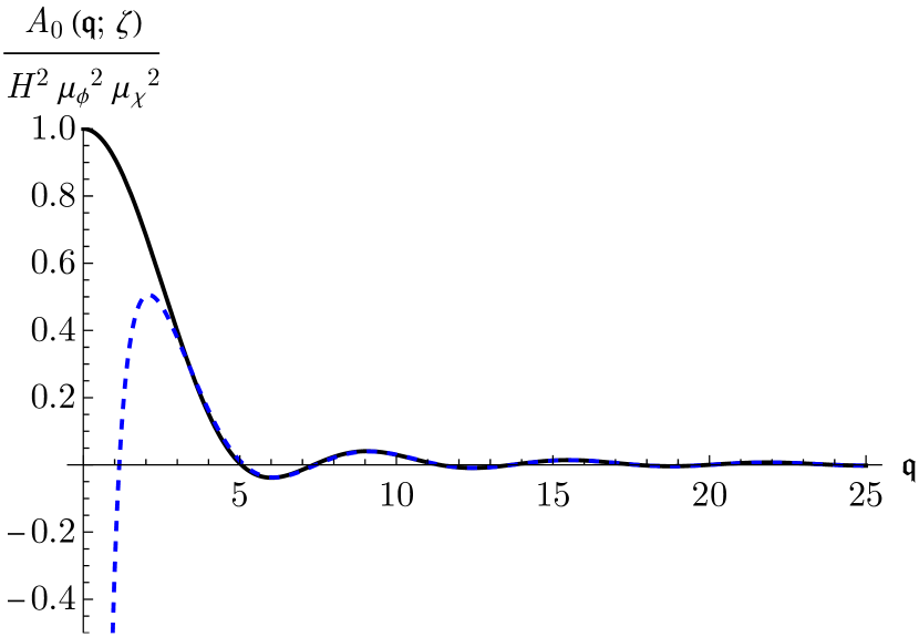
(a)

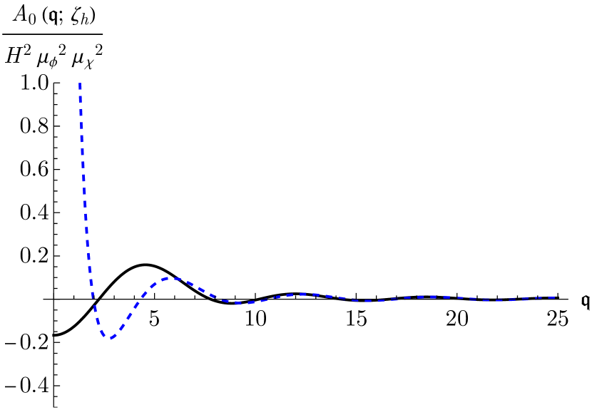
(b)

Figure 3: The amplitude $A_{0}(\mathfrak{q};\zeta)$ in $d=4$ for several values of $\zeta$. Left panel: $A_{0}(\zeta=1)$. Right panel: $A_{0}(\zeta=\zeta_{h})$. For $\mathfrak{q}=0$, the amplitude attains the finite value given in (53). For large $\mathfrak{q}$, the amplitude behaves as $\sim\mathfrak{q}^{-2}\left(1-\alpha\cos(\mathfrak{q})\right)$, as computed in (56). This approximation is depicted by the dashed blue lines.

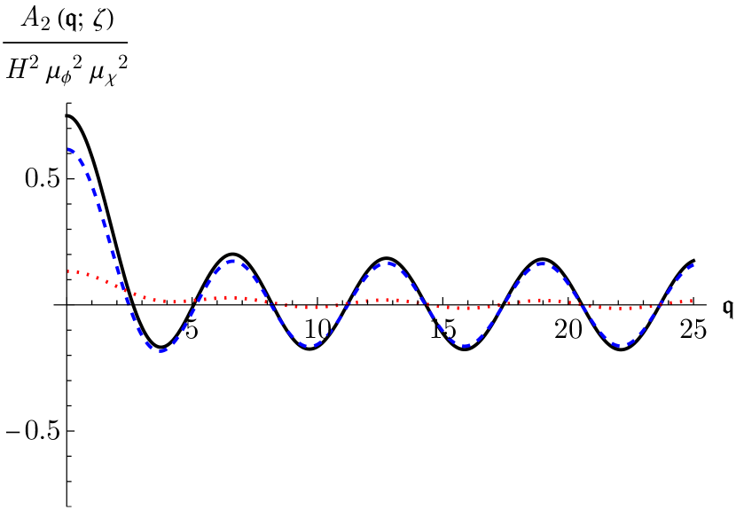
(a)

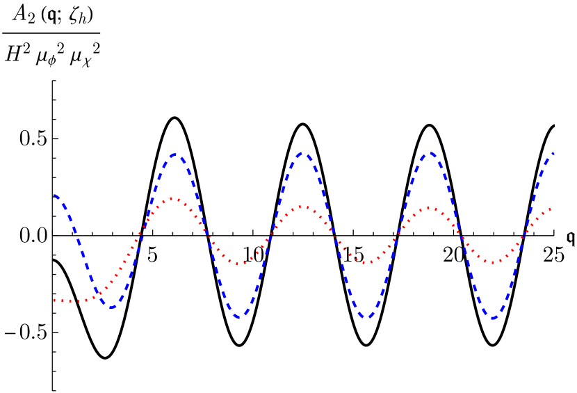
(b)

Figure 4: The amplitude $A_{2}(\mathfrak{q};\zeta)$ in $d=4$ for several values of $\zeta$. Left panel: $A_{2}(\zeta=1)$. Right panel: $A_{2}(\zeta=\zeta_{h})$. Solid line: the total amplitude $A_{2}$. Dashed blue line: $A_{2}^{\text{reg}}$. Dotted red line: $A_{2}^{\text{sing}}$. For $\mathfrak{q}=0$, the amplitude attains the finite values given by (54) and (55). For large $\mathfrak{q}$, the amplitude behaves as $\sim\cos(\mathfrak{q})$, as computed in (57) and (58).

We distinguish two features of the amplitude. First, we note that since the hypergeometric function ${}_{1}\hskip-1.0ptF_{2}$ is bounded, the amplitude is bounded too. In particular, it attains a finite value for $\mathfrak{q}\to 0$. For $A_{0}$, we find

$$\frac{A_{0}(\mathfrak{q}=0;\zeta)}{H^{2}\mu_{\phi}^{2}\mu_{\chi}^{2}}=\frac{1}{\zeta}\,\text{.}$$ (53)

For $A_{2}$, we first consider the regular part $A_{2}^{\text{reg}}$. The limit $\mathfrak{q}\to 0$ reads

$$\frac{A_{2}^{\text{reg}}(\mathfrak{q}=0;\zeta)}{H^{2}\mu_{\phi}^{2}\mu_{\chi}^{2}}=\frac{2}{3}\frac{1}{\zeta+4}+\frac{3}{4}\frac{1}{\zeta}\,\text{,}$$ (54)

while for the singular part $A_{2}^{\text{sing}}$, we compute

$$\frac{A_{2}^{\text{sing}}(\mathfrak{q}=0;\zeta)}{H^{2}\mu_{\phi}^{2}\mu_{\chi}^{2}}=\frac{2}{3}\frac{1}{\zeta+4}\,\text{,}$$ (55)

holding both for $\zeta\neq\zeta_{h}$ and for $\zeta=\zeta_{h}$.

The second feature that we study is the behavior at large $\mathfrak{q}$. Expanding around $\mathfrak{q}=\infty$, we obtain for $A_{0}$:

$$\frac{A_{0}(\mathfrak{q};\zeta)}{H^{2}\mu_{\phi}^{2}\mu_{\chi}^{2}}\sim\frac{1}{\mathfrak{q}^{2}}+\frac{4}{\sqrt{\pi}\zeta}\Gamma\left(\tfrac{7}{4}-\tfrac{\nu(\zeta)}{2}\right)\Gamma\left(\tfrac{7}{4}+\tfrac{\nu(\zeta)}{2}\right)\frac{1}{\mathfrak{q}^{2}}\cos\left(\mathfrak{q}\right)\,\text{.}$$ (56)

Expanding $A_{2}^{\text{reg}}$ around large momentum transfer, we find

$$\frac{A_{2}^{\text{reg}}(\mathfrak{q},\zeta)}{H^{2}\mu_{\phi}^{2}\mu_{\chi}^{2}}\sim-\frac{1}{3\sqrt{\pi}}\frac{\Gamma\left(\tfrac{3}{4}-\tfrac{\nu(\zeta)}{2}\right)\Gamma\left(\tfrac{3}{4}+\tfrac{\nu(\zeta)}{2}\right)}{\zeta+4}\cos\left(\mathfrak{q}\right)\,\text{.}$$ (57)

The large-$\mathfrak{q}$ expansion of $A_{2}^{\text{sing}}$ reads

$$\frac{A_{2}^{\text{sing}}(\mathfrak{q};\zeta)}{H^{2}\mu_{\phi}^{2}\mu_{\chi}^{2}}\sim\begin{cases}\begin{aligned} \frac{2}{3\sqrt{\pi}}\frac{\Gamma\left(\tfrac{3}{4}-\tfrac{\nu(\zeta-\zeta_{h})}{2}\right)\Gamma\left(\tfrac{3}{4}+\tfrac{\nu(\zeta-\zeta_{h})}{2}\right)}{\zeta+4}\cos\left(\mathfrak{q}\right)\end{aligned}\,\text{,}&\zeta\neq\zeta_{h}\\ \\ \begin{aligned} \frac{397-360\log(2)}{1080}\cos\left(\mathfrak{q}\right)\end{aligned}\,\text{,}&\zeta=\zeta_{h}\end{cases}\,\text{.}$$ (58)

We therefore find the following behavior: for large $\mathfrak{q}$, the amplitudes are oscillating. Restoring dimensionful quantities, we find that the oscillating terms are suppressed by $H^{2}$. Carefully taking the limit $H\to 0$, which we will not further discuss here, allows to recover the flat-spacetime $1/\vec{q}^{2}$ behavior.

4.2.2 Interpretation of the amplitudes

We will now briefly discuss the interpretation of the limits $\mathfrak{q}\to 0$ and $\mathfrak{q}\to\infty$.

Let us first consider the small-momentum limit, which we find to be finite. This behavior is in line with the expectation that $z=\zeta H^{2}$ acts as a mass, similar to the limit $\vec{q}\to 0$ for a flat-spacetime massive propagator $\propto\frac{1}{\vec{q}^{2}+z}$. A special case arises when $\zeta=\zeta_{h}$. Then (53), (54) and (55) are manifestly finite. In flat spacetime, on the other hand, we have a massless propagator, $\frac{1}{\vec{q}^{2}}$, which is divergent in the limit $\vec{q}\to 0$. We therefore conclude that the background curvature acts as an infrared regulator.

The oscillations in the large-momentum limit were also observed in Ferrero:2021lhd in the context of GR. As discussed there, the oscillations are typical for propagators in de Sitter spacetime Arkani-Hamed:2015bza . Furthermore, the discrete values where the amplitude vanishes has an interesting interpretation in terms of a probability density. A node at momentum $\mathfrak{q}_{0}$ then implies that the exchange of a graviton with this momentum is forbidden. These momenta are equidistantly separated with distance $\Delta\mathfrak{q}=2\pi$. This discrete behavior is reminiscent of discrete transition probabilities associated to particles in a box. In this context, the Hubble volume then acts as the boundary within which gravitons can propagate.

5 Scattering potential in the adiabatic expansion

The amplitude $A(\mathfrak{q})$ represents the transition probability of the scattering process $\phi\chi\to\phi\chi$ with momentum transfer $\mathfrak{q}$. Converting to position space, we find the transition amplitude of the same scattering process, where the external states are now localized at well-determined spacetime positions. As a generalization of the Born approximation in flat spacetime, we interpret this object as the scattering potential.

5.1 Computation of the scattering potential

We obtain the transition amplitude in position space by taking the Fourier transform of (52). Preparing particle $\phi_{1}$ at position $\vec{x}_{1}$ and particle $\chi_{1}$ at position $\vec{x}_{2}$, the transition probability arising from the amplitude $A_{i}$ is given by

$$V_{i}(\vec{x}_{1},\vec{x}_{2})=\frac{1}{2\mu_{\phi}\mu_{\chi}}\int\frac{\differential[d-1]{\vec{\mathfrak{k}}_{1}}}{(2\pi)^{d-1}}\frac{\differential[d-1]{\vec{\mathfrak{p}}_{1}}}{(2\pi)^{d-1}}\mathrm{e}^{\mathrm{i}\vec{p}_{1}\cdot\vec{x}_{1}}\mathrm{e}^{\mathrm{i}\vec{k}_{1}\cdot\vec{x}_{2}}A_{i}(\mathfrak{q;\zeta})\,\text{.}$$ (59)

Here the dimensionless proper momenta $\vec{\mathfrak{p}}_{1}=-\eta\vec{p}_{1}$ and $\vec{\mathfrak{k}}_{1}$ such that $\vec{q}=\vec{p}_{1}-\vec{k}_{1}$ are integrated over to obtain an invariant expression. In addition, the prefactor of the integral is chosen such that the resulting potential is correctly normalized.

Performing the integral over $\vec{\mathfrak{k}}_{1}$ and the spherical part of $\vec{\mathfrak{p}}_{1}$, we find the dimensionless potential:

$$V_{i}(\vec{x}_{1},\vec{x}_{2}) =\delta^{d-1}(H\vec{x}_{2})V_{i}(\mathfrak{r})\,\text{,}$$ (60)

$$V_{i}(\mathfrak{r}) =\frac{1}{2\mu_{\phi}\mu_{\chi}}\frac{2^{2-d}\pi^{\frac{1-d}{2}}}{\Gamma\left(\frac{d-1}{2}\right)}\int_{0}^{\infty}\differential{\mathfrak{q}}\mathfrak{q}^{d-2}{}_{0}\hskip-0.5ptF_{1}\left(\frac{d-1}{2};-\frac{\mathfrak{q}^{2}\mathfrak{r}^{2}}{4}\right)A_{i}\left(\mathfrak{q}\right)\,\text{.}$$ (61)

Here, $\mathfrak{r}=\lVert\eta(\vec{x}_{1}-\vec{x}_{2})\rVert$ denotes the proper distance between the particles $\phi_{1}$ and $\chi_{1}$. Central in this computation is the integral

$$\int_{0}^{\infty}\differential{x}x^{s-1}{}_{0}\hskip-0.5ptF_{1}\left(\alpha;-ax\right){}_{1}\hskip-1.0ptF_{2}\left(n;\beta_{1},\beta_{2};-bx\right)\,\text{.}$$ (62)

This has the structure of a Mellin transform, and was studied in MILLER2001 . In order to compute the Fourier transform of the functions ${}_{1}^{\phantom{0}}\hskip-1.0ptF_{2}^{(0;i,j;0)}\left(a;b,\frac{d-1}{2};-\frac{\mathfrak{q}^{2}}{4}\right)$ in (50) and (51), we express the derivatives as the limit of a finite difference. Exchanging the Fourier transform with the limit, the finite difference is of the form (62).

The potential is given by a discontinuous function,

$$V_{i}(\mathfrak{r})=\begin{cases}V_{i}^{\mathfrak{r}<1}(\mathfrak{r})&\mathfrak{r}<1\\ 0&\mathfrak{r}>1\end{cases}\,\text{.}$$ (63)

The potentials $V_{i}^{\mathfrak{r}<1}$ are conveniently expressed in terms of the following functions, valid for $\mathfrak{r}<1$ and non-negative integers $n$ and $m$:

$$\mathcal{V}_{nm}(\mathfrak{r};\zeta) =\frac{2^{2-d}\pi^{\frac{1-d}{2}}}{\Gamma\left(\frac{d-1}{2}\right)}\int_{0}^{\infty}\differential{\mathfrak{q}}\,\mathfrak{q}^{d-2}{}_{0}\hskip-0.5ptF_{1}\left(\frac{d-1}{2};-\frac{\mathfrak{q}^{2}\mathfrak{r}^{2}}{4}\right){}_{1}\hskip-1.0pt\tilde{F}_{2}\left(n;\frac{d-1}{4}+m,\frac{\nu(\zeta)}{2};-\frac{\mathfrak{q}^{2}}{4}\right)$$ (64)

$$=\begin{aligned} &\pi^{\frac{1-d}{2}}\frac{\Gamma\left(\frac{d-1}{2}-n\right)}{\Gamma(n)}\frac{\Gamma\left(\frac{d-1}{4}+m-\frac{\nu(\zeta)}{2}\right)\Gamma\left(\frac{d-1}{4}+m+\frac{\nu(\zeta)}{2}\right)}{\Gamma\left(\frac{d-1}{4}+m-n-\frac{\nu(\zeta)}{2}\right)\Gamma\left(\frac{d-1}{4}+m-n+\frac{\nu(\zeta)}{2}\right)}\times\\ &\qquad\qquad\mathfrak{r}^{1-d+2n}{}_{2}\hskip-1.0pt\tilde{F}_{1}\left(\frac{5-d}{4}-m+n,\frac{\nu(\zeta)}{2};\frac{3-d}{2}+n;\mathfrak{r}^{2}\right)\\ &+\pi^{\frac{1-d}{2}}\frac{\Gamma\left(\frac{1-d}{2}+n\right)}{\Gamma(n)}\frac{\Gamma\left(\frac{d-1}{4}+m-\frac{\nu(\zeta)}{2}\right)\Gamma\left(\frac{d-1}{4}+m+\frac{\nu(\zeta)}{2}\right)}{\Gamma\left(\frac{1-d}{4}+m-\frac{\nu(\zeta)}{2}\right)\Gamma\left(\frac{1-d}{4}+m+\frac{\nu(\zeta)}{2}\right)}\times\\ &\qquad\qquad{}_{2}\hskip-1.0pt\tilde{F}_{1}\left(\frac{d+3}{4}-m,\frac{\nu(\zeta)}{2};\frac{d+1}{2}-n;\mathfrak{r}^{2}\right)\,\text{.}\end{aligned}$$

In this expression, we defined ${}_{2}\hskip-1.0pt\tilde{F}_{1}\left(a,b;c;z\right)={}_{2}\hskip-1.0ptF_{1}\left(a-b,a+b;c;z\right)$ in terms of a hypergeometric function. It is now straightforward to express the $V_{i}^{\mathfrak{r}<1}$ in terms of $\mathcal{V}_{nm}$. For $V_{0}$, we find

$$V_{0}^{\mathfrak{r}<1}(\mathfrak{r};\zeta)=\frac{\mu_{\phi}\mu_{\chi}}{2\zeta}\mathcal{V}_{1,1}(\mathfrak{r};\zeta)\,\text{.}$$ (65)

Similar to $A_{2}$, the potential $V_{2}^{\mathfrak{r}<1}$ splits into a regular and a singular part:

$$V_{2}(\mathfrak{r};\zeta)=V_{2}^{\text{reg}}(\mathfrak{r})+V_{2}^{\text{sing}}(\mathfrak{r})\,\text{.}$$ (66)

The regular part is given by

$$V_{2}^{\text{reg}}(\mathfrak{r};\zeta)=\begin{aligned} \frac{\mu_{\phi}\mu_{\chi}}{2(\zeta+d)}\Bigg{[}\frac{1}{d-1}\mathcal{V}_{1,0}(\mathfrak{r};\zeta)+\left[\frac{d-3}{\zeta}-\frac{1}{d}\right]\mathcal{V}_{1,1}(\mathfrak{r},\zeta)+\frac{2}{\zeta}\mathcal{V}_{2,1}(\mathfrak{r};\zeta)\Bigg{]}\,\text{,}\end{aligned}$$ (67)

while the singular part becomes

$$V_{2}^{\text{sing}}(\mathfrak{r};\zeta)=\begin{cases}\begin{aligned} \frac{\mu_{\phi}\mu_{\chi}}{2(\zeta+d)}\frac{d-2}{d-1}\mathcal{V}_{1,0}(\mathfrak{r};\zeta-\zeta_{h})\,\text{,}\end{aligned}&\zeta\neq\zeta_{h}\\ \\ \begin{aligned} -\frac{\mu_{\phi}\mu_{\chi}}{2}\left[\frac{1}{d-1}\mathcal{V}_{1,0}(\mathfrak{r};0)+\frac{\pi^{\frac{1-d}{2}}}{2}\Gamma\left(\frac{d+1}{2}\right)\right]\,\text{,}\end{aligned}&\zeta=\zeta_{h}\end{cases}\,\text{.}$$ (68)

The function $V_{2}^{\text{sing}}(\mathfrak{r};\zeta=\zeta_{h})$ reduces to the rational function

$$V_{2}^{\text{sing}}(\mathfrak{r};\zeta=\zeta_{h})=\frac{\mu_{\phi}\mu_{\chi}}{2}\pi^{\frac{1-d}{2}}\Gamma\left(\frac{d-1}{2}\right)\frac{\mathfrak{r}^{3-d}+\frac{1}{4}-\mathfrak{r}^{2}-\frac{1}{4}(d+\mathfrak{r}^{2}-d\mathfrak{r}^{2})^{2}}{(d-1)(\mathfrak{r}-1)^{2}(\mathfrak{r}+1)^{2}}\,\text{.}$$ (69)

The total, dimensionful scattering potential for QuadG can easily be expressed in terms of the $V_{i}$. For $\mathfrak{r}<1$, we have

$$V^{\mathfrak{r}<1}(\mathfrak{r})=16\pi G_{N}H^{3}\,c(\alpha_{R},\alpha_{E})\bigg{[} -\frac{\zeta_{C}+d}{\zeta_{C}-\zeta_{h}}\Big{(}V_{2}(\mathfrak{r};\zeta_{h})-V_{2}(\mathfrak{r};\zeta_{C})\Big{)}$$ (70)

$$+\frac{1}{d(d-1)}\frac{\zeta_{C}}{\zeta_{C}-\zeta_{h}}\Big{(}V_{0}(\mathfrak{r};\zeta_{h})-V_{0}(\mathfrak{r};\zeta_{C})\Big{)}$$

$$+\frac{1}{(d-1)(d-2)}\Big{(}V_{0}(\mathfrak{r};\zeta_{h})-V_{0}(\mathfrak{r};\zeta_{R})\Big{)}\bigg{]}\,\text{,}$$

while the potential is equal to zero for $\mathfrak{r}>1$.

5.2 Properties of the potential

Having computed the potential for QuadG in (70), we will now consider its phenomenological properties. To this end, we will regard the potential as the source of a Newtonian force. In accordance with the classical Newtonian dynamics we define the gravitational force as $F=-\nabla V(r)$.

This allows to straightforwardly interpret the potential in terms of potential energies, and the scaling of the force with distance.

5.2.1 The short-distance regime

We will first consider the regime $\mathfrak{r}\ll 1$. In this region, spacetime can be approximated as locally flat, so that we expect curvature effects to be negligible. Hence, in this limit we should recover the behavior of the potential in Minkowski spacetime. The Yukawa-like potential of QuadG is easily obtained from the Minkowski-spacetime scattering amplitude, and reads

$$V_{\text{Mink}}(r)=G_{N}m_{\phi}m_{\chi}\left(-\frac{1}{r}-\frac{1}{3}\frac{1}{r}\mathrm{e}^{-r/\sqrt{\alpha_{R}}}+\frac{4}{3}\frac{1}{r}\mathrm{e}^{-r/\sqrt{\alpha_{C}}}\right)$$ (71)

For de Sitter spacetime, there are four cases to be considered:

General relativity

In this case, the higher-derivative couplings $\alpha_{R}$ and $\alpha_{C}$ are both zero. Upon expanding around $\mathfrak{r}=0$, we then find

$$V_{\text{GR}}(\mathfrak{r})\sim-G_{N}H^{3}\frac{\mu_{\phi}\mu_{\chi}}{\mathfrak{r}}\,\text{.}$$ (72)

Hence, we reproduce Newton’s law, as is discussed in detail in Ferrero:2021lhd .

$R^{2}$-gravity

We continue with $R^{2}$-gravity, obtained from the limit (29). In this case, the $\mathfrak{r}\to 0$ behavior reads

$$V_{R^{2}}(\mathfrak{r})\sim-\frac{4}{3}\frac{\zeta_{R}}{\zeta_{R}+4}G_{N}H^{3}\frac{\mu_{\phi}\mu_{\chi}}{\mathfrak{r}}\,\text{.}$$ (73)

This is in agreement with the short-distance behavior for $R^{2}$-gravity in flat spacetime, determined by (71).

At this point, a remark about Newton’s constant $G_{N}$ is in order. The numerical value of $G_{N}$ can be defined as the coefficient of the $1/r$ law, which can be obtained e.g. from a Cavendish experiment. For relativistic theories, one then determines numerical prefactors by taking the appropriate Newtonian limit, and comparing coefficients. The prime example of this is the prefactor $8\pi G_{N}$ on the right-hand side of the Einstein equation. Therefore, in the case of $R^{2}$-gravity, we can renormalize the constant $G_{N}$ such that we obtain exactly the Newtonian potential.

Hence, setting

$$\hat{G}_{\text{N}}=\begin{cases}\frac{4}{3}\frac{\zeta_{R}}{\zeta_{R}+4}G_{N}\,\text{,}&0<\zeta_{R}<\infty\\ \\ G_{N}&\text{otherwise}\end{cases}\,\text{,}$$ (74)

we conclude that also $R^{2}$-gravity yields a Newtonian force law at distances small compared to the Hubble length.

In order to distinguish $G_{N}$ from $\hat{G_{N}}$, the universal value of $G_{N}$ can be determined by performing a higher order scattering experiments involving more than two particles. We emphasize anyhow that this is unimportant for our purposes, aiming at studying the modifications to the Newtonian potential.

Furthermore, we note that in the limit $\alpha_{R}\to 0\;(\zeta_{R}\to\infty)$ a discontinuity arises. This discontinuity is reminiscent of the massive gravity vDVZ discontinuity vanDam:1970vg ; Zakharov:1970cc . This arises because of the different number of degrees of freedom in the two cases: the “massive” scalar field does not decouple properly in this limit.

$C^{2}$-gravity

We proceed with $C^{2}$-gravity, given by the limit (30). Expanding around $\mathfrak{r}=0$ gives

$$V_{C^{2}}(\mathfrak{r})\sim+\frac{1}{3}G_{N}H^{3}\frac{\mu_{\phi}\mu_{\chi}}{\mathfrak{r}}\,\text{,}$$ (75)

which is the same as what we find from (71). In contrast to GR and $R^{2}$-gravity, we find that $C^{2}$-gravity yields a repulsive force-law at short distances.

Quadratic gravity.

We finish our discussion of the short-distance regime by considering full QuadG. Here we find that the potential does not possess a pole at $\mathfrak{r}=0$, similar to what we find by evaluating (71) at $r=0$. The absence of such a short-distance singularity can be seen as the classical analogue of the perturbative renormalizability of QuadG, c.f. Stelle:1976gc ; Stelle:1977ry .

5.2.2 The de Sitter horizon

The second property of the potential that we discuss is the regime $\mathfrak{r}\sim 1$. As we have seen in (63), the potential vanishes at distances $\mathfrak{r}>1$. As was already observed in Ferrero:2021lhd , this is a natural manifestation of de Sitter horizon: since particles that are separated by the horizon are not in causal contact, their scattering potential must be identically zero.

In order to further study the discontinuity, we interpret $V$ as the source of a Newtonian force. We will be interested in the dimensionless quantity

$$\mathfrak{F}=-\frac{V^{\prime}(\mathfrak{r})}{\hat{G}_{\text{N}}H^{3}\mu_{\phi}\mu_{\chi}}\,\text{,}$$ (76)

which can be seen as the Newtonian force expressed in Hubble units.

It is clear that for radii $\mathfrak{r}>1$, the force $\mathfrak{F}$ is zero. Approaching $\mathfrak{r}=1$ from below, the discontinuity in $\mathfrak{F}$ can be computed Hawking:1975vcx ; Damour:1976jd ; Li:2016sjq . We find that the discontinuity lies in the interval

$$\lim_{\mathfrak{r}\nearrow 1}\mathfrak{F}_{\zeta\to 0}\leq\lim_{\mathfrak{r}\nearrow 1}\mathfrak{F}\leq\lim_{\mathfrak{r}\nearrow 1}\mathfrak{F}_{\text{GR}}\,\text{,}$$ (77)

where $\mathfrak{F}_{\text{GR}}$ is the force for General Relativity and $\mathfrak{F}_{\zeta\to 0}$ is the force of QuadG in the limit $\zeta_{C},\zeta_{R}\to 0$. These values can be computed exactly:

$$\lim_{\mathfrak{r}\nearrow 1}\mathfrak{F}_{\zeta\to 0} =-\frac{17}{24}-\frac{5\Gamma\left(\frac{3}{4}-\frac{\nu(\zeta_{h})}{2}\right)\Gamma\left(\frac{3}{4}+\frac{\nu(\zeta_{h})}{2}\right)}{6\sqrt{\pi}}+\frac{4\Gamma\left(\frac{3}{4}-\frac{\nu(-\zeta_{h})}{2}\right)\Gamma\left(\frac{3}{4}+\frac{\nu(-\zeta_{h})}{2}\right)}{3\sqrt{\pi}}$$ (78)

$$\approx 1.647\,\text{;}$$

$$\lim_{\mathfrak{r}\nearrow 1}\mathfrak{F}_{\text{GR}} =\frac{5}{6}+\frac{5\Gamma\left(\frac{3}{4}-\frac{\nu(\zeta_{h})}{2}\right)\Gamma\left(\frac{3}{4}+\frac{\nu(\zeta_{h})}{2}\right)}{3\sqrt{\pi}}$$

$$\approx 3.443\,\text{.}$$

We notice that both values are positive. Hence, at the de Sitter horizon, the net gravitational force is repulsive, in contrast to classical Newtonian gravity. We interpret this as an effect of the positive curvature: the expansion of the universe manifests itself as a repulsive effective force.

5.2.3 MOND from quadratic gravity

We now study $\mathfrak{F}$ in the intermediate regime $0<\mathfrak{r}<1$. We will pay special attention to the comparison to the classical Newtonian force $\mathfrak{F}_{\text{cl}}=-\mathfrak{r}^{-2}$. Any deviation from this potential can be seen as an instance of Modified Newtonian Dynamics (MOND). In recent years, phenomenological models of MOND have been constructed to explain rotation curves of galaxies, which do not correspond to classical Newtonian gravity Mannheim:2010xw ; Milgrom:2011kx ; Famaey:2011kh ; 2016PhRvL.117t1101M ; OBRIEN2018433 ; deAlmeida:2018kwq ; Mannheim:2021mhj ; MANNHEIM2006340 ; Brouwer:2021nsr . MOND is therefore an alternative to Dark Matter (DM) models, which explain the discrepancy of galactic rotation curves by the existence of non-luminous cold matter.

In order to reproduce a DM-like scenario using MOND, one mimics the additional mass density by modifying the potential such that one obtains an additional attractive force. In this section, we will consider whether such a modification can arise from $\mathfrak{F}$ by an appropriate choice of $\zeta_{C}$ and $\zeta_{R}$. Again, we distinguish four different regimes.

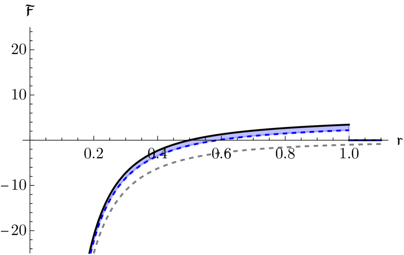
(a)

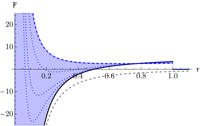
(b)

Figure 5: Dimensionless forces $\mathfrak{F}$ in $R^{2}$- and $C^{2}$-gravity. In both panels, the black curve denotes $\mathfrak{F}_{\text{GR}}$, while the dashed gray curve shows the classical Newtonian force $\mathfrak{F}_{\text{cl}}=-\mathfrak{r}^{-2}$ for reference. Left panel: $\mathfrak{F}$ in $R^{2}$-gravity. Scanning over $\zeta_{R}$, the curves $\mathfrak{F}_{\zeta_{R}}$ fill the shaded blue region, bounded by $\mathfrak{F}_{\text{GR}}$ and $\mathfrak{F}_{\zeta_{R}\to 0}$ (dashed blue curve). Right panel: $\mathfrak{F}$ in $C^{2}$-gravity. Scannosning over $\zeta_{C}$ fills the shaded blue region, bounded by $\mathfrak{F}_{\text{GR}}$ and $\mathfrak{F}_{\zeta_{C}\to 0}$ (dashed blue curve). For typical finite values of $\zeta_{C}$, $\mathfrak{F}$ is drawn using dotted blue curves. Both for $R^{2}$- and $C^{2}$-gravity, the force is strictly larger than $\mathfrak{F}_{\text{cl}}$, indicating that a dark matter MOND-like scenario is excluded.

General relativity

We begin with GR. The force $\mathfrak{F}_{\text{GR}}$ is shown by the black curve in Figure 5. Comparing $\mathfrak{F}_{\text{GR}}$ to the classical Newtonian force $\mathfrak{F}_{\text{cl}}=-\mathfrak{r}^{-2}$ (the dashed gray curve in Figure 5), we observe that the two coincide for small $\mathfrak{r}$, as discussed previously. Also the discontinuity is clearly visible. Furthermore, we observe that $\mathfrak{F}_{\text{GR}}$ is strictly larger than $\mathfrak{F}_{\text{class}}$. Hence, the spacetime curvature causes an additional expanding force, coinciding with the expectation that de Sitter spacetime models an expanding universe.

$R^{2}$-gravity

Turning on the coupling $\alpha_{R}$, we find that the addition of an $R^{2}$-interaction gives a modification to General Relativity. Letting $\zeta_{R}$ run from $0$ to $\infty$, we find that the curves $\mathfrak{F}$ fill the shaded blue region in the left panel of Figure 5. Here the dashed blue line denotes the limiting case $\mathfrak{F}_{\zeta_{R}\to 0}$. We find that the $R^{2}$ modification causes $\mathfrak{F}$ to be lower than $\mathfrak{F}_{\text{GR}}$. Hence, the $R^{2}$-interaction effectively causes an attractive force on top of the force due to GR. However, the modification is nowhere strong enough to give rise to DM-like MOND.

$C^{2}$-gravity

In the right panel of Figure 5, the force arising from $C^{2}$-gravity is shown. Similar to $R^{2}$-gravity, varying $\zeta_{C}$ traces out a region bounded by $\mathfrak{F}_{\text{GR}}$ and $\mathfrak{F}_{\zeta_{C}\to 0}$. In contrast to $R^{2}$-gravity, $\mathfrak{F}$ is always positive for sufficiently small $\mathfrak{r}$, due to the $+\mathfrak{r}^{-1}$-like behavior of the potential. In fact, below $\mathfrak{r}\approx 0.770$, $\mathfrak{F}$ is strictly larger than $\mathfrak{F}_{\text{GR}}$. Therefore, in this regime the effect of the $C^{2}$-interaction can be interpreted as an additional repulsive force on top of General Relativity. Thus, $C^{2}$-gravity cannot be matched to a MOND-potential suitable to explain DM.

Quadratic gravity

Finally, we consider full QuadG. As we have seen, since the potential of QuadG is finite at $\mathfrak{r}=0$, there will be no $\mathfrak{r}^{-2}$-like behavior of $\mathfrak{F}$. Instead, we find that $\mathfrak{F}\sim-\frac{3}{2}-\frac{\zeta_{C}}{2}+\frac{\zeta_{R}}{8}$ for small $\mathfrak{r}$. Thus, by an appropriate choice of $\zeta_{C}$ and $\zeta_{R}$, the force $\mathfrak{F}$ can reach any finite value at $\mathfrak{r}=0$. This includes $\mathfrak{F}=0$, which can be related to force laws arising from spacetimes with higher regularity Bonanno:2000ep . We find that $\mathfrak{F}$ is mostly bounded by $\mathfrak{F}_{\zeta_{R}\to 0}$ and $\mathfrak{F}_{\zeta_{C}\to 0}$ (the shaded blue region in Figure 6). For $\mathfrak{r}\gtrsim 0.770$, the force is bounded by $\mathfrak{F}_{\text{GR}}$ and $\mathfrak{F}_{\zeta\to 0}$, obtained by taking the limit $\lim_{\zeta_{C},\zeta_{R}\to 0}\mathfrak{F}$. This is shown in detail in the right panel of Figure 6.

Thus, we conclude that no choice of $\zeta_{C}$ and $\zeta_{R}$ gives rise to an effective force that is more attractive than the classical Newtonian force. Instead, we find in the entire parameter space a repulsive contribution to the gravitational force. Therefore, de Sitter curvature corrections to QuadG cannot explain galactic rotation curves.

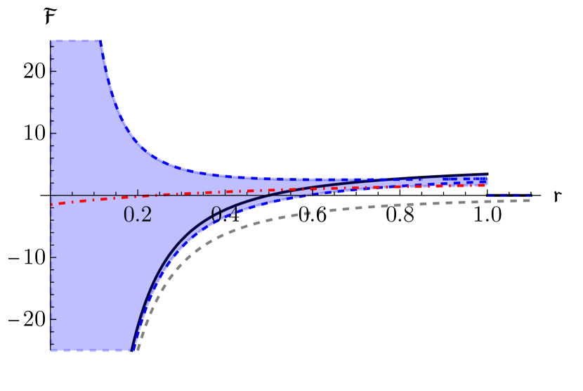
(a)

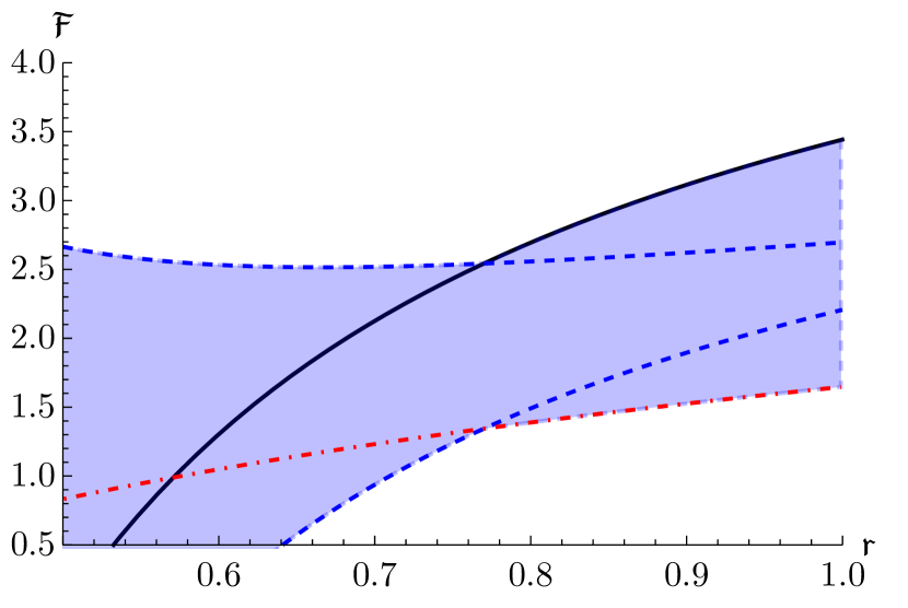
(b)

Figure 6: Dimensionless forces $\mathfrak{F}$ in QuadG. The black curve denotes $\mathfrak{F}_{\text{GR}}$. The dashed gray curve shows the classical Newtonian force $\mathfrak{F}_{\text{cl}}=-\mathfrak{r}^{-2}$. For any point in the shaded blue region, there exist values of $\zeta_{C}$, $\zeta_{R}$ such that this point is reached by $\mathfrak{F}_{\zeta_{C},\zeta_{R}}$. In particular, for any $\zeta_{C},\zeta_{R}$, $\mathfrak{F}$ reaches a finite value at $\mathfrak{r}=0$. The shaded blue region is bounded by $\mathfrak{F}_{\text{GR}}$, $\mathfrak{F}_{\zeta_{R}\to 0}$, $\mathfrak{F}_{\zeta_{C}\to 0}$ (dashed blue lines), and $\mathfrak{F}_{\zeta\to 0}$ (dashed-dotted red line). The right panel shows a detail of the left panel, clarifying the boundary of the shaded region near the de Sitter horizon.

6 Conclusion

In Ferrero:2021lhd , we introduced a covariant framework to compute Green’s functions and potentials in de Sitter spacetime. In this follow-up paper, we extend the formalism to include non-minimal interactions. More specifically, we considered the tree-level scattering of two scalar fields in quadratic gravity, given by $R^{2}$- and $C^{2}$-terms in the action, in addition to the Einstein-Hilbert action with cosmological constant. Apart from a kinetic term and mass term, the action for the scalar fields is given by an $R\phi\phi$ interaction.

After having reviewed the derivation of the Yukawa potential in Section 2, in Section 3 we constructed the Green’s functional for this scattering process. In addition to be fully covariant, we showed that the on-shell Green’s functional is explicitly gauge-independent. We organized the propagator and vertices in such a way that an effective mass-pole structure for rank-0 and rank-2 vertex tensors could be identified. Novel in this setting are corrections to the poles due to the de Sitter curvature, parameterized by the parameters $\zeta_{C}$, $\zeta_{R}$ and $\zeta_{h}$. We observed that in the case of conformally coupled scalars, only the rank-2 vertex tensor $T_{\mu\nu}$ contributes.

In order to extract the explicit expression of the tree-level amputated Green’s function, we considered the adiabatic limit of the Green’s functional in Section 4. This limit is implemented as an expansion in a large mass of the scalar fields compared to the Hubble constant, i.e., as an expansion in $\mu_{\phi}^{-1}$ and $\mu_{\chi}^{-1}$. This expansion allows to use spatial momentum techniques to evaluate the Green’s functional. We performed this analysis for any mass parameter $\zeta$ of the graviton propagator, necessary to cover quadratic gravity. It turns out that the mass parameter $\zeta_{h}$, which represents the usual value of the mass parameter associated to the massless graviton in a de Sitter spacetime Garidi:2003ys ; Pejhan:2018ofn ; Joung:2006gj ; Joung:2007je , is special, in the sense that the amplitude for this mass parameter is not continuously connected to the amplitude corresponding to different masses.

Analogous to what has been found in the GR case Ferrero:2021lhd , the amplitude of quadratic gravity presents an oscillating behavior as a function of the proper transferred momentum $\mathfrak{q}$, giving rise to an amplitude vanishing for periodic discrete values. This feature is attributed to the presence of the horizon in a de Sitter spacetime: the particles are bounded to interact within an Hubble volume. Furthermore, the amplitude is finite for $\mathfrak{q}\to 0$, similar to the behavior of a mass term in a flat-spacetime massive propagator. In particular, this holds too for $\zeta=\zeta_{h}$, corresponding to a regularization of the amplitude due to a nonzero $H$. This is in contrast to the flat-spacetime case, where a massless graviton propagator gives rise to a divergent amplitude in the limit $q\to 0$.

We then took in Section 5 the Fourier transform of the amplitude to obtain the scattering potential. For small proper separations $\mathfrak{r}$, we find a potential that is in agreement with the flat-spacetime Yukawa potentials. Generalizing the result in Ferrero:2021lhd , we found that the potential at super-Hubble distances is exactly zero: there is not causal interaction between particles separated by the de Sitter horizon. At the horizon $\mathfrak{r}=1$, we computed the $\zeta$-dependent discontinuity in the potential.

Interpreting the scattering potential as the source of a Newtonian force, we investigated whether the modified potentials in quadratic gravity could give rise to Modified Newtonian Dynamics corresponding to dark-matter like rotation curves. However, we report that the de Sitter curvature gives rise to an effective repulsive force that cannot be matched to a dark-matter like scenario.

Along this treatment, in order to obtain the classical nonrelativistic potential, the choice of the boundary conditions is not important. However, this choice should be resolved in order to construct causal and relativistic observables.

This program for computing de Sitter spacetime Green’s function can be investigated further in a number of ways. First, it is interesting to extract the amplitude and potential for conformally coupled scalar fields. An initial investigation of this system shows that this gives rise to a modification of the differential equations determining the amplitude. Currently it is unknown whether this system of equations can be solved.

Moreover, we can investigate the Green’s function by extending adiabatic expansion. Expanding up to second order in the $\mu_{\phi}^{-1}$ and $\mu_{\chi}^{-1}$ would furnish information about the dependence of the amplitude on the scattering angle, which is usually encoded in the post-Newtonian (non-relativistic) expansion. Secondly, in order to take into account off-shell quantum corrections, it would be instructive to consider loop Feynman diagrams. An efficient way of organizing these quantum effects is by using form factors Knorr:2022dsx .

Further investigation of the discontinuity may also shed more light on the properties of the de Sitter horizon. In the present work, the discontinuity arises as a result of the Fourier transform. Here, special care has to be taken in integrating over the momentum $\mathfrak{q}$ in the presence of the expansion in $\mu_{\phi}$ and $\mu_{\chi}$. A computation of the potential in a system where the adiabatic expansion is not needed, e.g., for conformally coupled scalars, could give more insight into the behavior of the potential around $\mathfrak{r}=1$.

In addition, this may also yield information regarding the thermodynamic properties of the de Sitter horizon. A potential with curvature-induced modifications may accommodate additional particle states, which may be given an interpretation in terms of particle production. This can then be compared to the de Sitter temperature of the horizon.

Finally, this covariant construction of Green’s functionals can be extended to other curved backgrounds that also admit an adiabatic expansion, such as FLRW spacetimes. In particular, can be applied in the slow-roll inflationary spacetimes. A comparison to $n$-point functions imprinted in the Cosmic Microwave Background would allow to make contact with astrophysical observations.

Appendix A Conventions

In this Appendix, we collect some basic facts about de Sitter spacetime. The $d$-dimensional de Sitter spacetime is uniquely characterized as the maximally symmetric Lorentzian manifold with constant positive scalar curvature. The Ricci curvature tensor is given by

$$R_{\mu\nu}=\frac{R}{d}g_{\mu\nu}\,\text{,}$$ (79)

where $R>0$ is the constant scalar curvature. The Weyl tensor vanishes. It is convenient to introduce the Hubble constant $H>0$:

$$R=d(d-1)H^{2}\,\text{.}$$ (80)

De Sitter spacetime is conformally flat, which means that it is conformal to the Minkowski metric:

$$\differential{s^{2}}=\frac{1}{(H\eta)^{2}}\left(-\differential{\eta^{2}}+\differential{x_{1}^{2}}+\cdots+\differential{x_{d-1}^{2}}\right)\,\text{.}$$ (81)

In our conventions, $\eta$ runs from $-\infty$ to $0$, corresponding to past and future infinity, respectively.

Appendix B The adiabatic expansion

Here we compile several facts about the adiabatic expansion in de Sitter spacetime that were previously derived in Ferrero:2021lhd . In general, adiabaticity assumes that the curvature of spacetime is much smaller than the scales associated to the processes taking place in it Agullo:2014ica ; Moreno-Pulido:2022phq ; Junker:2001gx ; Lueders:1990np ; Olbermann:2007gn ; Fulling1979RemarksOP ; Fulling:1974zr ; Fulling:1989nb ; Parker:1968mv ; Parker:1969au ; Parker:1971pt ; Parker:1974qw ; Parker:2009uva ; Birrell_adiabatic ; Bunch_adiabatic ; Bunch:1978aq ; Haro:2008zz ; Winitzki:2005rw ; Zeldovich1 ; Zeldovich2 . For quantum field theory in curved spacetime, the adiabatic expansion has the advantage that it does not rely on a strict definition of asymptotic states Marolf:2012kh . This is of particular interest in our work.

In the case of scalar particle scattering in de Sitter spacetime, the adiabatic expansion is implemented concretely by performing an expansion in $\mu^{-1}=H/m$, where $m$ is the mass of the scalar field and $H$ the Hubble parameter. Essentially, in this expansion the Compton frequency of the scalar fields is assumed to be much larger than the expansion rate of de Sitter spacetime.

This expansion is applied to the wave functions of the scalar fields. In the conformal coordinates (81) solutions to the Klein-Gordon equation are labeled by the comoving momentum $\vec{p}$ and are given by Bunch ; Mukhanov:2007zz :

$$h_{\vec{p},\mu}(\eta,\vec{x})=\eta^{\frac{d-1}{2}}H^{(1)}_{\mathrm{i}\sqrt{\mu^{2}-\left(\frac{d-1}{2}\right)^{2}}}(-p\eta)\mathrm{e}^{\mathrm{i}\vec{p}\cdot\vec{x}}\,\text{.}$$ (82)

Here, $H^{(1)}_{\nu}(z)$ is the Hankel function of the first kind olver10 .

This particular choice for parameterizing the solutions to the Klein-Gordon equation leads to the Bunch-Davies vacuum Bunch ; Birrell ; Mukhanov:2007zz . This generalizes the Minkowski vacuum to de Sitter spacetime by two features: it is the unique choice of solutions such that firstly the coefficients of the corresponding creation and annihilation operators are complex conjugates, and secondly such that an expansion around $\mu=\infty$ exists.

In order to expand (82) in large $\mu$, we compute the expansion of $H^{(1)}_{\mathrm{i}\mu}(z)$ for large $\mu$. We observe that since the Hankel functions are solutions to Bessel’s equation

$$z^{2}H^{\prime\prime}(z)+zH^{\prime}(z)+(z^{2}+\mu^{2})H(z)=0\,\text{,}$$ (83)

one can expand the equation by making the ansatz that the derivative of $H$ can be expressed in terms of $H$ itself, i.e.,

$$H^{\prime}(z)=f(z)H(z)\,\text{.}$$ (84)

This turns Bessel’s equation (83) to the nonlinear equation

$$z^{2}f^{\prime}(z)+z^{2}f(z)^{2}+zf(z)+z^{2}+\mu^{2}=0\,\text{.}$$ (85)

Seeking a solution that has at most a simple pole in $\mu^{-1}$, the following ansatz for $f$ is in order:

$$f(z)=\mu\sum_{n\geq 0}f_{n}(z)\mu^{-n}\,\text{.}$$ (86)

Plugging this back into (85), we are now able to solve the differential equation order by order in $\mu$. The first few equations are explicitly:

$$0 =1+z^{2}f_{0}^{2}\,\text{,} 0=f_{0}+2zf_{0}f_{1}+zf_{0}^{\prime}\,\text{,}$$ (87)

$$0 =z^{2}+z^{2}f_{1}^{2}+2z^{2}f_{0}f_{2}+z^{2}f_{1}^{\prime}\,\text{,} 0=f_{2}+2zf_{1}f_{2}+2zf_{0}f_{3}+zf_{2}^{\prime}\,\text{.}$$

Solving these equations furnish the expansion in terms of $\mu^{-1}$:

$$f_{\pm}(z)=\pm\frac{\mathrm{i}\mu}{z}\pm\frac{\mathrm{i}z}{2\mu}-\frac{z}{2\mu^{2}}-\pm\frac{\mathrm{i}z(4+z^{2})}{8\mu^{3}}+\order{\mu^{-4}}\,\text{.}$$ (88)

We now have to show that this solution of (85) indeed gives an expansion of the Hankel functions. To this end, we expand $H^{(1)}_{\mathrm{i}\mu}(z)$ first around $z=0$, and subsequently around $\mu=\infty$. This gives

$$H^{(1)}_{\mathrm{i}\mu}(z)=\frac{\mathrm{i}\mu}{z}+\order{z,\mu^{-1}}\,\text{.}$$ (89)

We note that this expansion matches exactly the first term of $f_{+}$ hence $f_{+}$ represents indeed the expansion of $H^{(1)}_{\mathrm{i}\mu}$.

With this expansion at hand, it is straightforward to compute the action of derivative operators acting on the mode functions (82). In particular, we have time derivative

$$\partial_{\eta}h_{\vec{p},\mu}=\left[\frac{\mathrm{i}\mu}{\eta}+\frac{d-1}{\eta}+\mathrm{i}\left(\frac{1}{2}p^{2}\eta^{2}-\frac{(d-1)^{2}}{8\eta}\right)\frac{1}{\mu}+\order{\mu^{-2}}\right]h_{\vec{p},\mu}\,\text{.}$$ (90)

This formula lies at the basis of the expansion of, e.g., the action of the graviton propagator $\mathcal{G}(\square)$ on the vertex tensors $V$ and $T_{\mu\nu}$ used in this work.

Appendix C Computational details of the Green’s function in the adiabatic expansion

In this Appendix, we assemble several details regarding the calculation of the scattering amplitude. First, we discuss the existence of the expansion of the vertex tensors $V$ and $T_{\mu\nu}$ in the adiabatic limit $\mu^{-1}\to 0$. Second, we will provide additional details regarding the adiabatic expansion of the propagator.

C.1 Adiabatic expansion of the vertices

Having studied the adiabatic limit of a single scalar field in Appendix B, we now consider the adiabatic expansion of the vertex tensors $V$ and $T_{\mu\nu}$. Computing the action of $\square$ on $\chi_{1}\chi_{2}$ using (90), we find that the vertex $V[\chi_{1},\chi_{2}]$ expands to

$$V[\chi_{1},\chi_{2}]=\left[H^{2}\mu_{\chi}^{2}+\order{\mu_{\chi}^{0}}\right]\chi_{1}\chi_{2}\,\text{.}$$ (91)

Thus, the terms $\mathcal{A}_{0}(\zeta)$ will each contribute to leading order $\mu_{\chi}^{2}$ to the Green’s function. For the tensor vertex $T_{\mu\nu}$, we compute the components

$$T_{00}[\chi_{1},\chi_{2}] =\left[\frac{d+1}{d}\frac{1}{\eta^{2}}\,\mu_{\chi}^{2}+\order{\mu_{\chi}^{0}}\right]\chi_{1}\chi_{2}\,\text{,}$$ (92)

$$T_{0i}[\chi_{1},\chi_{2}] =\left[\frac{1}{2\eta}(k_{1,i}+k_{2,i})\,\mu_{\chi}+\order{\mu_{\chi}^{0}}\right]\chi_{1}\chi_{2}\,\text{,}$$

$$T_{ij}[\chi_{1},\chi_{2}] =\left[\frac{1}{d\eta^{2}}\delta_{ij}\,\mu_{\chi}^{2}+\order{\mu_{\chi}^{0}}\right]\chi_{1}\chi_{2}\,\text{.}$$

Note that the (00)-component and the $(ij)$-components are of order $\mu_{\chi}^{2}$. Therefore, only these will contribute to the leading order in the adiabatic expansion of $\mathcal{A}_{2}(\zeta)$.

C.2 Expansion of the propagator

We proceed by showing that the action of the propagator on the scalar fields also has a well-behaved adiabatic expansion. We will show this explicitly for the scalar vertex $V$; for the tensor vertex $T_{\mu\nu}$, the procedure is completely analogous.

First, we show that $f(\square)\phi_{1}\phi_{2}$ has an expansion in $\mu_{\phi}^{-1}$ for any analytic function $f$. Since $f$ has a Taylor series expansion, it suffices to show that the expansion exists for $\square^{n}\phi_{1}\phi_{2}$. This is shown by an inductive argument. First, we note that for $n=0$, we have trivially

$$\square^{n}\phi_{1}\phi_{2}=\phi_{1}\phi_{2}\equiv\left[\alpha_{0}(\eta)+\order{\mu_{\phi}^{-1}}\right]\phi_{1}\phi_{2}\,\text{,}$$ (93)

namely for $\alpha_{0}(\eta)=1$. We now make the inductive assumption that (93) holds for $n\geq 0$. Then acting with one more d’Alembertian gives

$$\square^{n+1}\phi_{1}\phi_{2}=\square\left(\alpha_{n}(\eta)\phi_{1}\phi_{2}\right)=\left[\left(q^{2}\eta^{2}\alpha_{n}+d\eta\alpha_{n}^{\prime}+\eta^{2}\alpha_{n}^{\prime\prime}\right)H^{2}+\order{\mu_{\phi}^{-1}}\right]\phi_{1}\phi_{2}\,\text{.}$$ (94)

Here, the prime denotes a derivative with respect to $\eta$. By induction, it follows that $\square^{n}\phi_{1}\phi_{2}$ is $\order{\mu_{\phi}^{0}}\phi_{1}\phi_{2}$ for any $n$. Therefore, for any function $f$ that admits an analytic expansion, $f(\square)\phi_{1}\phi_{2}$ can be expanded to zeroth order in $\mu_{\phi}^{-1}$.

Analogously, one proves that $f(\square)T_{\mu\nu}$ has a well-defined expansion, by taking care of the tensor structure of $T_{\mu\nu}$. Here, the leading order is $\order{\mu_{\phi}^{2}}$, cf. (92).

We note from (94) that $\square^{n}\phi_{1}\phi_{2}$ also contains $n$ powers of $q^{2}\eta^{2}=\mathfrak{q}^{2}$. Thus, we conclude that the expansion of $f(\square)\phi_{1}\phi_{2}$ is automatically analytic in $\mathfrak{q}$.

In particular, this is true for the propagator. Representing $(\square+z)^{-1}$ as a geometric series,

$$(\square+z)^{-1}=\frac{1}{z}\sum_{n=0}^{\infty}\left(\frac{-\square}{z}\right)^{n}\,\text{,}$$ (95)

we see that for $z\neq 0$ the propagator has an analytic expansion. Thus, we require the adiabatic expansion of the propagator in $\mu_{\phi}^{-1}$ to be analytic in $\mathfrak{q}$.

As a consequence, the solution to the differential equation (39) is fixed. Since this is a second-order inhomogeneous differential equation, one would expect the solution to be formed an inhomogeneous solution, accompanied by a two-dimensional homogeneous solution space. However, since the homogeneous solutions are generally not analytic, we will discard these in this paper.

References

- (1) N. Aghanim, Y. Akrami, M. Ashdown, J. Aumont, C. Baccigalupi, M. Ballardini et al., Planck 2018 results, Astronomy and Astrophysics 641 (2020) A6.
- (2) Supernova Cosmology Project collaboration, Measurements of and from 42 high redshift supernovae, Astrophys. J. 517 (1999) 565 [astro-ph/9812133].
- (3) Supernova Search Team collaboration, Observational evidence from supernovae for an accelerating universe and a cosmological constant, Astron. J. 116 (1998) 1009 [astro-ph/9805201].
- (4) J.D. Barrow and D.J. Shaw, The Value of the Cosmological Constant, Gen. Rel. Grav. 43 (2011) 2555 [1105.3105].
- (5) J. Martin, Everything You Always Wanted To Know About The Cosmological Constant Problem (But Were Afraid To Ask), Comptes Rendus Physique 13 (2012) 566 [1205.3365].
- (6) G. ’t Hooft and M.J.G. Veltman, One loop divergencies in the theory of gravitation, Ann. Inst. H. Poincare Phys. Theor. A 20 (1974) 69.
- (7) M.H. Goroff and A. Sagnotti, Quantum Gravity at two loops, Phys. Lett. B160 (1985) 81.
- (8) M.H. Goroff and A. Sagnotti, The Ultraviolet Behavior of Einstein Gravity, Nucl. Phys. B266 (1986) 709.
- (9) J. Polchinski, String Theory, vol. 1 of Cambridge Monographs on Mathematical Physics, Cambridge University Press (1998), 10.1017/CBO9780511816079.
- (10) D. Tong, String Theory, 0908.0333.
- (11) C. Rovelli, Loop quantum gravity, Living Rev. Rel. 1 (1998) 1 [gr-qc/9710008].
- (12) B. Dittrich and T. Thiemann, Testing the master constraint programme for loop quantum gravity. I. General framework, Class. Quant. Grav. 23 (2006) 1025 [gr-qc/0411138].
- (13) C. Wetterich, Exact evolution equation for the effective potential, Phys. Lett. B 301 (1993) 90 [1710.05815].
- (14) M. Reuter, Nonperturbative evolution equation for quantum gravity, Phys.Rev. D57 (1998) 971 [hep-th/9605030].
- (15) M. Reuter and F. Saueressig, Quantum Gravity and the Functional Renormalization Group, Cambridge University Press (2019).
- (16) R. Percacci, An Introduction to Covariant Quantum Gravity and Asymptotic Safety, vol. 3 of 100 Years of General Relativity, World Scientific (2017), 10.1142/10369.
- (17) A. Eichhorn, An asymptotically safe guide to quantum gravity and matter, Front. Astron. Space Sci. 5 (2019) 47 [1810.07615].
- (18) J.M. Pawlowski and M. Reichert, Quantum Gravity: A Fluctuating Point of View, Front. in Phys. 8 (2021) 551848 [2007.10353].
- (19) R. Ferrero and M. Reuter, The spectral geometry of de Sitter space in asymptotic safety, JHEP 08 (2022) 040 [2203.08003].
- (20) J. Ambjorn, A. Goerlich, J. Jurkiewicz and R. Loll, Nonperturbative Quantum Gravity, Phys. Rept. 519 (2012) 127 [1203.3591].
- (21) R. Loll, Quantum Gravity from Causal Dynamical Triangulations: A Review, Class. Quant. Grav. 37 (2020) 013002 [1905.08669].
- (22) J.F. Donoghue, Leading quantum correction to the Newtonian potential, Phys. Rev. Lett. 72 (1994) 2996 [gr-qc/9310024].
- (23) H.W. Hamber and S. Liu, On the quantum corrections to the Newtonian potential, Phys. Lett. B 357 (1995) 51 [hep-th/9505182].
- (24) N.E.J. Bjerrum-Bohr, J.F. Donoghue and B.R. Holstein, Quantum gravitational corrections to the nonrelativistic scattering potential of two masses, Phys. Rev. D 67 (2003) 084033 [hep-th/0211072].
- (25) M. Carrillo-González, C. de Rham and A.J. Tolley, Scattering amplitudes for binary systems beyond GR, JHEP 11 (2021) 087 [2107.11384].
- (26) N.E.J. Bjerrum-Bohr, P.H. Damgaard, L. Plante and P. Vanhove, Chapter 13: Post-Minkowskian expansion from scattering amplitudes, J. Phys. A 55 (2022) 443014 [2203.13024].
- (27) D.A. Kosower, R. Monteiro and D. O’Connell, Chapter 14: Classical gravity from scattering amplitudes, J. Phys. A 55 (2022) 443015 [2203.13025].
- (28) B. Allen, Vacuum states in de sitter space, Phys. Rev. D 32 (1985) 3136.
- (29) N.D. Birrell and P.C.W. Davies, Quantum Fields in Curved Space, Cambridge Monographs on Mathematical Physics, Cambridge University Press (1982), 10.1017/CBO9780511622632.
- (30) V. Mukhanov and S. Winitzki, Introduction to quantum effects in gravity, Cambridge University Press (6, 2007).
- (31) E.T. Akhmedov, U. Moschella and F.K. Popov, Characters of different secular effects in various patches of de Sitter space, Phys. Rev. D 99 (2019) 086009 [1901.07293].
- (32) E. Witten, Quantum gravity in de Sitter space, in Strings 2001: International Conference, 6, 2001 [hep-th/0106109].
- (33) R. Bousso, Cosmology and the S-matrix, Phys. Rev. D 71 (2005) 064024 [hep-th/0412197].
- (34) D. Marolf, I.A. Morrison and M. Srednicki, Perturbative S-matrix for massive scalar fields in global de Sitter space, Class. Quant. Grav. 30 (2013) 155023 [1209.6039].
- (35) S. Mandal and S. Banerjee, Local description of S-matrix in quantum field theory in curved spacetime using Riemann-normal coordinate, Eur. Phys. J. Plus 136 (2021) 1064 [1908.06717].
- (36) S.B. Giddings and R.A. Porto, The Gravitational S-matrix, Phys. Rev. D 81 (2010) 025002 [0908.0004].
- (37) C. de Rham, S. Kundu, M. Reece, A.J. Tolley and S.-Y. Zhou, Snowmass White Paper: UV Constraints on IR Physics, in 2022 Snowmass Summer Study, 3, 2022 [2203.06805].
- (38) B. Allen, Graviton propagator in de sitter space, Physical review D: Particles and fields 34 (1987) 3670.
- (39) B. Allen, The graviton propagator in homogeneous and isotropic spacetimes, Nuclear Physics 287 (1987) 743.
- (40) B. Allen and M. Turyn, An evaluation of the graviton propagator in de sitter space, Nuclear Physics 292 (1987) 813.
- (41) E.G. Floratos, J. Iliopoulos and T.N. Tomaras, Tree Level Scattering Amplitudes in De Sitter Space Diverge, Phys. Lett. B 197 (1987) 373.
- (42) L.H. Ford and L. Parker, Infrared divergences in a class of robertson-walker universes, Phys. Rev. D 16 (1977) 245.
- (43) I. Antoniadis and E. Mottola, Four-dimensional quantum gravity in the conformal sector, Phys. Rev. D 45 (1992) 2013.
- (44) E.T. Akhmedov, IR divergences and kinetic equation in de Sitter space. Poincare patch: Principal series, JHEP 01 (2012) 066 [1110.2257].
- (45) E.T. Akhmedov, Lecture notes on interacting quantum fields in de Sitter space, Int. J. Mod. Phys. D 23 (2014) 1430001 [1309.2557].
- (46) E.T. Akhmedov, K.V. Bazarov, D.V. Diakonov, U. Moschella, F.K. Popov and C. Schubert, Propagators and Gaussian effective actions in various patches of de Sitter space, Phys. Rev. D 100 (2019) 105011 [1905.09344].
- (47) E.T. Akhmedov, K.V. Bazarov, D.V. Diakonov and U. Moschella, Quantum fields in the static de Sitter universe, Phys. Rev. D 102 (2020) 085003 [2005.13952].
- (48) K. Lochan, K. Rajeev, A. Vikram and T. Padmanabhan, Quantum correlators in Friedmann spacetimes: The omnipresent de Sitter spacetime and the invariant vacuum noise, Phys. Rev. D 98 (2018) 105015 [1805.08800].
- (49) S. Singh, C. Ganguly and T. Padmanabhan, Quantum field theory in de Sitter and quasi–de Sitter spacetimes revisited, Phys. Rev. D 87 (2013) 104004 [1302.7177].
- (50) S.P. Kim, Vacuum Structure of de Sitter Space, 1008.0577.
- (51) J. Bros, U. Moschella and J.P. Gazeau, Quantum field theory in the de Sitter universe, Phys. Rev. Lett. 73 (1994) 1746.
- (52) J. Bros and U. Moschella, Two point functions and quantum fields in de Sitter universe, Rev. Math. Phys. 8 (1996) 327 [gr-qc/9511019].
- (53) J. Bros, H. Epstein and U. Moschella, Analyticity properties and thermal effects for general quantum field theory on de Sitter space-time, Commun. Math. Phys. 196 (1998) 535 [gr-qc/9801099].
- (54) A. Higuchi, D. Marolf and I.A. Morrison, On the Equivalence between Euclidean and In-In Formalisms in de Sitter QFT, Phys. Rev. D 83 (2011) 084029 [1012.3415].
- (55) A. Higuchi and R.H. Weeks, The Physical graviton two point function in de Sitter space-time with S3 spatial sections, Class. Quant. Grav. 20 (2003) 3005 [gr-qc/0212031].
- (56) M. Fukuma, S. Sugishita and Y. Sakatani, Propagators in de Sitter space, Phys. Rev. D 88 (2013) 024041 [1301.7352].
- (57) N. Arkani-Hamed and J. Maldacena, Cosmological Collider Physics, 1503.08043.
- (58) N. Arkani-Hamed, D. Baumann, H. Lee and G.L. Pimentel, The Cosmological Bootstrap: Inflationary Correlators from Symmetries and Singularities, JHEP 04 (2020) 105 [1811.00024].
- (59) S. Cacciatori, V. Gorini, A. Kamenshchik and U. Moschella, Conservation laws and scattering for de Sitter classical particles, Class. Quant. Grav. 25 (2008) 075008 [0710.0315].
- (60) R. Ferrero and C. Ripken, De Sitter scattering amplitudes in the Born approximation, SciPost Phys. 13 (2022) 106 [2112.03766].
- (61) E. Pechlaner and R. Sexl, On quadratic Lagrangians in general relativity, Communications in Mathematical Physics 2 (1966) 165 .
- (62) P. Havas, On theories of gravitation with higher-order field equations., General Relativity and Gravitation 8 (1977) 631.
- (63) J.F. Donoghue and G. Menezes, On quadratic gravity, Nuovo Cim. C 45 (2022) 26 [2112.01974].
- (64) A. Salvio, Metastability in Quadratic Gravity, Phys. Rev. D 99 (2019) 103507 [1902.09557].
- (65) A.A. Starobinsky, A New Type of Isotropic Cosmological Models Without Singularity, Phys. Lett. B 91 (1980) 99.
- (66) S.V. Ketov and A.A. Starobinsky, Inflation and non-minimal scalar-curvature coupling in gravity and supergravity, JCAP 08 (2012) 022 [1203.0805].
- (67) A.S. Koshelev, K. Sravan Kumar and A.A. Starobinsky, inflation to probe non-perturbative quantum gravity, JHEP 03 (2018) 071 [1711.08864].
- (68) A.S. Koshelev, K. Sravan Kumar, A. Mazumdar and A.A. Starobinsky, Non-Gaussianities and tensor-to-scalar ratio in non-local R2-like inflation, JHEP 06 (2020) 152 [2003.00629].
- (69) A. Vilenkin, Classical and Quantum Cosmology of the Starobinsky Inflationary Model, Phys. Rev. D 32 (1985) 2511.
- (70) C.P.L. Berry and J.R. Gair, Linearized f(R) Gravity: Gravitational Radiation and Solar System Tests, Phys. Rev. D 83 (2011) 104022 [1104.0819].
- (71) J.A.R. Cembranos, Dark Matter from R2-gravity, Phys. Rev. Lett. 102 (2009) 141301 [0809.1653].
- (72) D.J. Kapner, T.S. Cook, E.G. Adelberger, J.H. Gundlach, B.R. Heckel, C.D. Hoyle et al., Tests of the gravitational inverse-square law below the dark-energy length scale, Phys. Rev. Lett. 98 (2007) 021101 [hep-ph/0611184].
- (73) K.S. Stelle, Renormalization of Higher Derivative Quantum Gravity, Phys. Rev. D 16 (1977) 953.
- (74) K.S. Stelle, Classical Gravity with Higher Derivatives, Gen. Rel. Grav. 9 (1978) 353.
- (75) M.V. OstrogradskyMem. Ac. St. Petersbourg VI 4 (1850) 385.
- (76) I. Antoniadis and E.T. Tomboulis, Gauge invariance and unitarity in higher-derivative quantum gravity, Phys. Rev. D 33 (1986) 2756.
- (77) E. Tomboulis, 1/N Expansion and Renormalization in Quantum Gravity, Phys. Lett. B 70 (1977) 361.
- (78) J.F. Donoghue and G. Menezes, Unitarity, stability, and loops of unstable ghosts, Phys. Rev. D 100 (2019) 105006.
- (79) L.M. Sokolowski, Stability of a metric f(R) gravity theory implies the Newtonian limit, Acta Phys. Polon. B 39 (2008) 2879 [0810.2554].
- (80) S. Capozziello and A. Stabile, The Newtonian limit of metric gravity theories with quadratic Lagrangians, Class. Quant. Grav. 26 (2009) 085019 [0903.3238].
- (81) J. Naf and P. Jetzer, On the 1/c Expansion of f(R) Gravity, Phys. Rev. D 81 (2010) 104003 [1004.2014].
- (82) A. Conroy, T. Koivisto, A. Mazumdar and A. Teimouri, Generalized quadratic curvature, non-local infrared modifications of gravity and Newtonian potentials, Class. Quant. Grav. 32 (2015) 015024 [1406.4998].
- (83) L. Alvarez-Gaume, A. Kehagias, C. Kounnas, D. Lüst and A. Riotto, Aspects of Quadratic Gravity, Fortsch. Phys. 64 (2016) 176 [1505.07657].
- (84) J. Edholm, A.S. Koshelev and A. Mazumdar, Behavior of the Newtonian potential for ghost-free gravity and singularity-free gravity, Phys. Rev. D 94 (2016) 104033 [1604.01989].
- (85) C. Cheung, I.Z. Rothstein and M.P. Solon, From Scattering Amplitudes to Classical Potentials in the Post-Minkowskian Expansion, Phys. Rev. Lett. 121 (2018) 251101 [1808.02489].
- (86) M. Milgrom, A modification of the newtonian dynamics as a possible alternative to the hidden mass hypothesis, The Astrophysical Journal 270 (1983) 365.
- (87) M. Milgrom, MOND–particularly as modified inertia, Acta Phys. Polon. B 42 (2011) 2175 [1111.1611].
- (88) B. Famaey and S. McGaugh, Modified Newtonian Dynamics (MOND): Observational Phenomenology and Relativistic Extensions, Living Rev. Rel. 15 (2012) 10 [1112.3960].
- (89) A.O.F. de Almeida, L. Amendola and V. Niro, Galaxy rotation curves in modified gravity models, JCAP 08 (2018) 012 [1805.11067].
- (90) M.M. Brouwer et al., The weak lensing radial acceleration relation: Constraining modified gravity and cold dark matter theories with KiDS-1000, Astron. Astrophys. 650 (2021) A113 [2106.11677].
- (91) R.H. Sanders, Mass discrepancies in galaxies: dark matter and alternatives, The Astronomy and Astrophysics Review 2 (1990) 1.
- (92) L. Blanchet and J. Novak, Testing MOND in the Solar System, in 46th Rencontres de Moriond on Gravitational Waves and Experimental Gravity, pp. 295–302, 5, 2011 [1105.5815].
- (93) D. Brizuela, J.M. Martin-Garcia and G.A. Mena Marugan, xPert: Computer algebra for metric perturbation theory, Gen. Rel. Grav. 41 (2009) 2415 [0807.0824].
- (94) J.M. Martín-García, xperm: fast index canonicalization for tensor computer algebra, CoRR abs/0803.0862 (2008) [0803.0862].
- (95) T. Nutma, xTras : A field-theory inspired xAct package for mathematica, Comput. Phys. Commun. 185 (2014) 1719 [1308.3493].
- (96) “xAct: Efficient tensor computer algebra for Mathematica.” http://xact.es/index.html.
- (97) B. Knorr and C. Ripken, Scattering amplitudes in affine gravity, Phys. Rev. D 103 (2021) 105019 [2012.05144].
- (98) T. Garidi, What is mass in de Sitterian physics?, hep-th/0309104.
- (99) H. Pejhan, K. Bamba, S. Rahbardehghan and M. Enayati, Massless spin-2 field in de Sitter space, Phys. Rev. D 98 (2018) 045007 [1803.02074].
- (100) E. Joung, J. Mourad and R. Parentani, Group theoretical approach to quantum fields in de Sitter space. I. The Principle series, JHEP 08 (2006) 082 [hep-th/0606119].
- (101) E. Joung, J. Mourad and R. Parentani, Group theoretical approach to quantum fields in de Sitter space. II. The complementary and discrete series, JHEP 09 (2007) 030 [0707.2907].
- (102) G. Sengör and C. Skordis, Unitarity at the Late time Boundary of de Sitter, JHEP 06 (2020) 041 [1912.09885].
- (103) J.P. Gazeau and M. Lachieze Rey, Quantum field theory in de Sitter space: A Survey of recent approaches, PoS IC2006 (2006) 007 [hep-th/0610296].
- (104) M. Loparco, J. Penedones, K. Salehi Vaziri and Z. Sun, The Källén-Lehmann representation in de Sitter spacetime, 2306.00090.
- (105) N.C. Tsamis and R.P. Woodard, The Structure of perturbative quantum gravity on a De Sitter background, Commun. Math. Phys. 162 (1994) 217.
- (106) S. Park, T. Prokopec and R.P. Woodard, Quantum Scalar Corrections to the Gravitational Potentials on de Sitter Background, JHEP 01 (2016) 074 [1510.03352].
- (107) M.B. Fröb and E. Verdaguer, Quantum corrections to the gravitational potentials of a point source due to conformal fields in de Sitter, JCAP 03 (2016) 015 [1601.03561].
- (108) M.B. Fröb and E. Verdaguer, Quantum corrections for spinning particles in de Sitter, JCAP 04 (2017) 022 [1701.06576].
- (109) D. Glavan, S.P. Miao, T. Prokopec and R.P. Woodard, One-loop Graviton Corrections to Conformal Scalars on a de Sitter Background, Phys. Rev. D 103 (2021) 105022 [2007.10395].
- (110) J.F. Donoghue, General relativity as an effective field theory: The leading quantum corrections, Phys. Rev. D 50 (1994) 3874 [gr-qc/9405057].
- (111) I. Agullo, W. Nelson and A. Ashtekar, Preferred instantaneous vacuum for linear scalar fields in cosmological space-times, Phys. Rev. D 91 (2015) 064051 [1412.3524].
- (112) C. Moreno-Pulido and J.S. Peracaula, Renormalizing the vacuum energy in cosmological spacetime: implications for the cosmological constant problem, 2201.05827.
- (113) W. Junker and E. Schrohe, Adiabatic vacuum states on general space-time manifolds: Definition, construction, and physical properties, Annales Henri Poincare 3 (2002) 1113 [math-ph/0109010].
- (114) C. Lueders and J.E. Roberts, Local quasiequivalence and adiabatic vacuum states, Commun. Math. Phys. 134 (1990) 29.
- (115) H. Olbermann, States of low energy on Robertson-Walker spacetimes, Class. Quant. Grav. 24 (2007) 5011 [0704.2986].
- (116) S.A. Fulling, Remarks on positive frequency and hamiltonians in expanding universes, General Relativity and Gravitation 10 (1979) 807.
- (117) S.A. Fulling and L. Parker, Renormalization in the theory of a quantized scalar field interacting with a robertson-walker spacetime, Annals Phys. 87 (1974) 176.
- (118) S.A. Fulling, Aspects of Quantum Field Theory in Curved Space-time, vol. 17 (1989).
- (119) L. Parker, Particle creation in expanding universes, Phys. Rev. Lett. 21 (1968) 562.
- (120) L. Parker, Quantized fields and particle creation in expanding universes. 1., Phys. Rev. 183 (1969) 1057.
- (121) L. Parker, Quantized fields and particle creation in expanding universes. 2., Phys. Rev. D 3 (1971) 346.
- (122) L. Parker and S.A. Fulling, Adiabatic regularization of the energy momentum tensor of a quantized field in homogeneous spaces, Phys. Rev. D 9 (1974) 341.
- (123) L.E. Parker and D. Toms, Quantum Field Theory in Curved Spacetime: Quantized Field and Gravity, Cambridge Monographs on Mathematical Physics, Cambridge University Press (8, 2009), 10.1017/CBO9780511813924.
- (124) N.D. Birrell, The Application of Adiabatic Regularization to Calculations of Cosmological Interest, Proceedings of the Royal Society of London Series A 361 (1978) 513.
- (125) T.S. Bunch, Adiabatic regularisation for scalar fields with arbitrary coupling to the scalar curvature, Journal of Physics A Mathematical General 13 (1980) 1297.
- (126) T.S. Bunch, S.M. Christensen and S.A. Fulling, Massive Quantum Field Theory in Two-Dimensional Robertson-Walker Space-Time, Phys. Rev. D 18 (1978) 4435.
- (127) J. Haro and E. Elizalde, On particle creation in the flat FRW chart of de Sitter spacetime, J. Phys. A 41 (2008) 372003.
- (128) S. Winitzki, Cosmological particle production and the precision of the WKB approximation, Phys. Rev. D 72 (2005) 104011 [gr-qc/0510001].
- (129) Y. Zel’Dovich and A. Starobinsky, Particle production and vacuum polarization in an anisotropic gravitational field, Soviet Journal of Experimental and Theoretical Physics 34 (1972) 1159.
- (130) Y.B. Zel’dovich and A.A. Starobinsky, Rate of particle production in gravitational fields, JETP Lett. 26 (1977) 252.
- (131) H. Goodhew, Rational Wavefunctions in de Sitter Spacetime, 2210.09977.
- (132) G. Frobenius, Ueber die integration der linearen differentialgleichungen durch reihen., Journal für die reine und angewandte Mathematik 76 (1873) 214.
- (133) A.R. Miller, The mellin transform of a product of two hypergeometric functions, Journal of Computational and Applied Mathematics 137 (2001) 77.
- (134) H. van Dam and M.J.G. Veltman, Massive and massless Yang-Mills and gravitational fields, Nucl. Phys. B 22 (1970) 397.
- (135) V.I. Zakharov, Linearized gravitation theory and the graviton mass, JETP Lett. 12 (1970) 312.
- (136) S.W. Hawking, Particle Creation by Black Holes, Commun. Math. Phys. 43 (1975) 199.
- (137) T. Damour and R. Ruffini, Black Hole Evaporation in the Klein-Sauter-Heisenberg-Euler Formalism, Phys. Rev. D 14 (1976) 332.
- (138) W.-D. Li, Y.-Z. Chen and W.-S. Dai, Scattering state and bound state of scalar field in Schwarzschild spacetime: Exact solution, Annals Phys. 409 (2019) 167919 [1612.02644].
- (139) P.D. Mannheim and J.G. O’Brien, Fitting galactic rotation curves with conformal gravity and a global quadratic potential, Phys. Rev. D 85 (2012) 124020 [1011.3495].
- (140) S.S. McGaugh, F. Lelli and J.M. Schombert, Radial Acceleration Relation in Rotationally Supported Galaxies, Physical Review Letters 117 (2016) 201101 [1609.05917].
- (141) J.G. O’Brien, T.L. Chiarelli and P.D. Mannheim, Universal properties of galactic rotation curves and a first principles derivation of the tully–fisher relation, Physics Letters B 782 (2018) 433.
- (142) P.D. Mannheim and J.W. Moffat, External field effect in gravity, Int. J. Mod. Phys. D 30 (2021) 2142009 [2103.13972].
- (143) P.D. Mannheim, Alternatives to dark matter and dark energy, Progress in Particle and Nuclear Physics 56 (2006) 340.
- (144) A. Bonanno and M. Reuter, Renormalization group improved black hole space-times, Phys. Rev. D 62 (2000) 043008 [hep-th/0002196].
- (145) B. Knorr, C. Ripken and F. Saueressig, Form Factors in Asymptotically Safe Quantum Gravity, 2210.16072.
- (146) J. de Boer and S.N. Solodukhin, A Holographic reduction of Minkowski space-time, Nucl. Phys. B 665 (2003) 545 [hep-th/0303006].
- (147) D. Colosi, General boundary quantum field theory in de Sitter spacetime, 1010.1209.
- (148) C. Cheung, A. de la Fuente and R. Sundrum, 4D scattering amplitudes and asymptotic symmetries from 2D CFT, JHEP 01 (2017) 112 [1609.00732].
- (149) I. Park, Foliation-Based Approach to Quantum Gravity and Applications to Astrophysics, Universe 5 (2019) 71 [1902.03332].
- (150) A.A. Saharian, T.A. Petrosyan and V.S. Torosyan, Mean field squared and energy–momentum tensor for the hyperbolic vacuum in dS spacetime, Annals Phys. 437 (2022) 168728 [2110.06662].
- (151) T.S. Bunch and P.C.W. Davies, Quantum field theory in de Sitter space - Renormalization by point-splitting, Proceedings of the Royal Society of London Series A 360 (1978) 117.
- (152) F.W.J. Olver, D.W. Lozier, R.F. Boisvert and C.W. Clark, The NIST Handbook of Mathematical Functions, Cambridge Univ. Press (2010).
- (153) N. Birrell, Momentum space techniques for curved space-time quantum field theory, Proceedings of The Royal Society A: Mathematical, Physical and Engineering Sciences 367 (1979) 123.