Twin-width of random graphs

Abstract

We investigate the twin-width of the Erdős-Rényi random graph $G(n,p)$. We unveil a surprising behavior of this parameter by showing the existence of a constant $p^{*}\approx 0.4$ such that with high probability, when $p^{*}\leq p\leq 1-p^{*}$, the twin-width is asymptotically $2p(1-p)n$, whereas, when $p<p^{*}$ or $p>1-p^{*}$, the twin-width is significantly higher than $2p(1-p)n$. In particular, we show that the twin-width of $G(n,1/2)$ is concentrated around $n/2-(\sqrt{3n\log n})/2$ within an interval of length $o(\sqrt{n\log n})$. For the sparse random graph, we show that with high probability, the twin-width of $G(n,p)$ is $\Theta(n\sqrt{p})$ when $(726\ln n)/n\leq p\leq 1/2$.

1 Introduction

Twin-width is a graph parameter recently introduced by Bonnet, Kim, Thomassé, and Watrigant [9]. Typically, twin-width is defined in terms of contractions on trigraphs; see Section 2 for the formal definition. Equivalently, the twin-width of a graph, denoted by $\operatorname{tww}(G)$, is the minimum integer $d$ such that there is a way to move from the partition of the vertex set into parts having a single vertex each to the trivial partition having only one part consisting of all vertices by iteratively merging a pair of parts such that at every stage of the process, every part has both an edge and a non-edge to at most $d$ other parts. Such a sequence of partitions is equivalent to a $d$-contraction sequence. Graphs of twin-width $0$ are precisely cographs, which are graphs that can be built from $K_{1}$ by making disjoint unions and adding twins.

Twin-width is receiving a lot of attention not only because many interesting classes of graphs have bounded twin-width but also because in every class of graphs of bounded twin-width, any property expressible in first-order logic can be decided in linear time as long as the corresponding $d$-contraction sequence is given as an input [9]. Furthermore, every class of graphs of bounded twin-width admits a function $f$ such that the chromatic number of every graph $G$ in the class is bounded from above by $f(\omega(G))$, where $\omega(G)$ is the clique number of $G$ [4], which unifies and also simplifies known theorems on the $\chi$-boundedness of certain graph classes. Graphs of bounded tree-width, graphs of bounded clique-width, planar graphs, graphs embeddable on a fixed surface, and all proper minor-closed graph classes are proved to have bounded twin-width [9]. Twin-width has generated a huge amount of interests [9, 5, 4, 6, 7, 14, 8, 2, 13, 22, 10, 21, 15].

We investigate the twin-width of the Erdős-Rényi random graph $G(n,p)$, which is a graph on a vertex set $\{1,2,\ldots,n\}$ chosen randomly such that each unordered pair of vertices is adjacent with probability $p$ independently at random. Since the twin-width is invariant under taking the complement graph, we may focus on $G(n,p)$ with $p\leq 1/2$, because $G(n,p)$ and $G(n,1-p)$ have the same twin-width distribution. We say that $G(n,p)$ satisfies a property $\mathcal{P}$ with high probability if the probability that $\mathcal{P}$ holds on $G(n,p)$ converges to $1$ as $n$ goes to infinity.

First, we show that the twin-width of $G(n,p)$ is proportional to $n\sqrt{p}$ with high probability if $(726\ln n)/n\leq p\leq 1/2$ for all sufficiently large $n$. Previously, Ahn, Hendrey, Kim, and Oum [1] showed the following lower bound.

Theorem 1.1 (Ahn, Hendrey, Kim, and Oum [1]).

For every $\varepsilon>0$, if $p:=p(n)$ satisfies $1/n\leq p\leq 1/2$, then with high probability,

$$\operatorname{tww}(G(n,p))>2p(1-p)n-(2\sqrt{2}+\varepsilon)\sqrt{p(1-p)n\ln n}.$$

They also showed that the twin-width of an $n$-vertex graph is at most $n/2+o(n)$, and so when $1/n\leq p\leq 1/2$, the twin-width of $G(n,p)$ is between $(p-\varepsilon)n$ and $\frac{(1+\varepsilon)}{2}n$ with high probability for any positive constant $\varepsilon$. We improve this and determine that $n\sqrt{p}$ is the exact function when $p\geq(726\ln n)/n$.

Theorem 1.2.

Let $p:=p(n)$ such that $\frac{726\ln n}{n}\leq p(n)\leq 1/2$ for all sufficiently large $n$. With high probability, $\operatorname{tww}(G(n,p))=\Theta(n\sqrt{p})$.

Ahn, Hendrey, Kim, and Oum [1] computed thresholds for $\operatorname{tww}(G(n,p))\in\{0,1,2\}$. In particular, they showed that $\operatorname{tww}(G(n,p))\leq 2$ with high probability if $p\leq cn^{-1}$ for any constant $c\in(0,1)$. Determining the twin-width asymptotically when $\frac{1}{n}\leq p<\frac{726\ln n}{n}$ remains open. In Proposition 4.4, we will show that if $\omega(n^{-1})\leq p\leq 1/2$, then the twin-width of $G(n,p)$ is unbounded.

Second, we focus on the situation when $p$ is a non-zero constant. Each of Theorems 1.1 or 1.2 tells us that the twin-width of $G(n,p)$ grows linearly in $n$ for this case, but these theorems do not decide the coefficient of the linear term in $\operatorname{tww}(G(n,p))$. We show that there is a threshold $p^{*}\approx 0.4013$ such that if $0<p<p^{*}$, then there exists $c>0$ depending on $p$ such that with high probability,

$$\operatorname{tww}(G(n,p))>(2p(1-p)+c)n$$

and if $p^{*}<p\leq 1/2$, then with high probability,

$$\operatorname{tww}(G(n,p))=2p(1-p)n+o(n),$$

proving that the lower bound given by Theorem 1.1 is tight up to the first-order term in this case, and furthermore we also determine the second-order term of $\operatorname{tww}(G(n,p))$. We were told that Behague et al. [3] independently studied the twin-width of $G(n,p)$.

Theorem 1.3.

There exists $p^{*}\in(0.4012,0.4013)$ such that the following hold for a real $p$ and $q:=1-p$.

1. If $p^{*}<p\leq 1/2$, then with high probability,

   $$\operatorname{tww}(G(n,p))=2pqn-\sqrt{6pq(1-2pq)n\ln n}+o(\sqrt{n\ln n}).$$

2. If $0<p<p^{*}$, then there exists $c:=c(p)>0$ such that with high probability,

   $$\operatorname{tww}(G(n,p))>(2pq+c)n.$$

As a corollary, we deduce the following for $G(n,1/2)$.

Corollary 1.4.

The twin-width of $G(n,1/2)$ is $\frac{n}{2}-\frac{\sqrt{3n\ln n}}{2}+o(\sqrt{n\ln n})$ with high probability.

One natural question for a graph parameter is to determine its maximum value across all graphs with a fixed number of vertices. Ahn, Hendrey, Kim, and Oum [1] showed that the twin-width of an $n$-vertex graph is bounded from above by $n/2+\sqrt{n\ln n}/2+o(\sqrt{n\ln n})$ and proved that an $n$-vertex Paley graph has twin-width exactly $(n-1)/2$. They asked whether there exist $n$-vertex graphs of twin-width larger than $(n-1)/2$. Corollary 1.4 implies that the twin-width of the random graph $G(n,1/2)$ is far less than $(n-1)/2$, differing by at least $\Omega(\sqrt{n\ln n})$. This behavior of twin-width is different from that of the parameter of rank-width, denoted by $\operatorname{rw}(G)$, introduced by Oum and Seymour [20]. Like twin-width, rank-width is almost invariant under graph complementation; the rank-width of a graph and that of its complement differ by at most $1$. By definition, the rank-width of an $n$-vertex graph is bounded from above by $\lceil n/3\rceil$ and Lee, Lee, and Oum [17] showed that if $p\in(0,1)$ is a constant, then the rank-width of $G(n,p)$ is $\lceil n/3\rceil-O(1)$ with high probability. This means that unlike twin-width, the rank-width of $G(n,p)$ is with high probability within an additive constant of the maximum possible value.

We remark that the twin-width is not a monotonic parameter, meaning that the twin-width of a subgraph of a graph $G$ can be more than the twin-width of $G$. It is true however that if $p_{1}$ and $p_{2}$ are constant with $p^{*}<p_{1}<p_{2}\leq 1/2$, then $\operatorname{tww}(G(n,p_{1}))\leq\operatorname{tww}(G(n,p_{2}))$ with high probability by Theorem 1.3. Moreover, the upper bound arguments to prove Theorem 1.3 in Section 3 can also be used to show that if $p_{1}$ and $p_{2}$ are constant with $p_{1}\leq p^{*}<p_{2}\leq 1/2$, then $\operatorname{tww}(G(n,p_{1}))\leq\operatorname{tww}(G(n,p_{2}))$ with high probability. In fact, we suspect that this also holds when $p_{1}<p_{2}\leq p^{*}$, but this remains open.

Organization.

We organize this paper as follows. In Section 2, we introduce the definitions of a trigraph and twin-width, and summarize some standard terminology and results from graph theory and probability theory. Section 3 is devoted to the proof of the upper bound in Theorem 1.3(1). In Section 4, we prove lower bounds in Theorem 1.3 and prove Theorem 1.2. The proofs of some technical inequalities are relegated to the appendix.

2 Preliminaries

In this paper, all (tri)graphs are simple and finite. For a graph $G$ and two disjoint vertex sets $A$, $B\subseteq V(G)$, let $G[A]$ be the subgraph of $G$ whose vertex set is $A$ and whose edge set consists of all edges of $G$ not incident with a vertex in $V(G)\setminus A$. Let $G[A,B]$ be the bipartite subgraph of $G$ with $V(G[A,B])=A\cup B$ whose edge set consists of all edges in $G$ adjacent to one vertex in $A$ and another vertex in $B$. We denote by $\delta(G)$ the minimum degree of $G$ and by $\Delta(G)$ the maximum degree of $G$.

We start with a standard lemma that allows us to find a subgraph with large minimum degree of a given graph.

Proposition 2.1 (See Diestel [12, Proposition 1.2.2]).

Let $G$ be a graph with at least one edge. Then $G$ has a subgraph $H$ with minimum degree $\delta(H)>\lvert E(G)\rvert/\lvert V(G)\rvert$.

2.1 Twin-width

For a positive integer $t$ and a set $S$, $\binom{S}{t}$ is the set of all $t$-element subsets of $S$ and $[t]:=\{1,\ldots,t\}$. For sets $S$ and $T$, $S\triangle T:=(S\setminus T)\cup(T\setminus S)$ and is called the symmetric difference of $S$ and $T$.

A trigraph is a triple $G=(V,B,R)$ for disjoint sets $B,R\subseteq\binom{V}{2}$. For a trigraph $G=(V,B,R)$, we denote by $V(G):=V$ the set of vertices, by $B(G):=B$ the set of black edges, by $R(G):=R$ the set of red edges, and by $E(G):=B\cup R$ the set of edges. We identify a graph $H=(V,E)$ with a trigraph $H=(V,E,\emptyset)$. For a set $S\subseteq V(G)$, $G\setminus S$ is the trigraph obtained from $G$ by deleting the vertices in $S$ and the edges incident with vertices in $S$. If $S=\{v\}$, then we may write $G\setminus v$ for $G\setminus\{v\}$.

For a vertex $v$ of a trigraph $G$, the degree of $v$, denoted $\deg(v)$, is the number of edges of $G$ incident with $v$, and the red-degree of $v$, denoted $\operatorname{rdeg}(v)$, is the number of red edges of $G$ incident with $v$. Let $N_{G}^{R}(v)$ be the set of vertices $w$ such that $vw\in R(G)$ and let $\Delta\!^{R}(G)$ be the maximum red-degree of $G$.

For distinct vertices $u$ and $v$ of $G$, not necessarily adjacent, $G/\{u,v\}=(V^{\prime},B^{\prime},R^{\prime})$ is the trigraph such that for a new vertex $w\notin V$, we have that $V^{\prime}=(V\setminus\{u,v\})\cup\{w\}$ and $G\setminus\{u,v\}=(G/\{u,v\})\setminus w$, and for each $x\in V^{\prime}\setminus\{w\}$, the following hold:

1. $wx\in B^{\prime}$ if and only if $\{ux,vx\}\subseteq B$,

2. $wx\notin B^{\prime}\cup R^{\prime}$ if and only if $\{ux,vx\}\cap(B\cup R)=\emptyset$, and

3. $wx\in R^{\prime}$, otherwise.

We say that $G/\{u,v\}$ is obtained from $G$ by contracting $u$ and $v$. Let $r_{G}(u,v)$ be the red-degree of the new vertex in $G/\{u,v\}$ obtained by contracting $u$ and $v$. Note that if $G$ is a graph, then $r_{G}(u,v)=|(N_{G}(u)\triangle N_{G}(v))\setminus\{u,v\}|$.

A partial contraction sequence from $G_{1}$ to $G_{t}$ is a sequence $G_{1},\ldots,G_{t}$ of trigraphs such that for each $i\in[t-1]$, $G_{i+1}$ is obtained from $G_{i}$ by contracting two vertices. If $\Delta\!^{R}(G_{i})\leq d$ for every $i\in[t]$, then we call the sequence a partial $d$-contraction sequence. A contraction sequence of $G$ is a partial contraction sequence from $G$ to a $1$-vertex graph. A $d$-contraction sequence of $G$ is a partial $d$-contraction sequence from $G$ to a $1$-vertex graph. The twin-width of $G$ is the minimum $d$ such that there is a $d$-contraction sequence of $G$. We denote by $\operatorname{tww}(G)$ the twin-width of $G$.

For a partial contraction sequence $\sigma=G_{1},G_{2},\ldots,G_{t}$ from $G_{1}$ to $G_{t}$, we define a function $\sigma:V(G_{1})\to V(G_{t})$, using the same symbol with the sequence, as follows. For each $v\in V(G_{1})$, $\sigma(v):=v$ if $v$ is not contracted, and otherwise $\sigma(v)$ is the vertex of $G_{t}$ to which $v$ is contracted. For a set $S\subseteq V(G_{t})$, $\sigma^{-1}(S)$ is the preimage of $S$ under $\sigma$. If $S=\{v\}$, then we may write $\sigma^{-1}(v)$ for $\sigma^{-1}(\{v\})$. For $s\in[t]$ and a positive integer $i$, we denote by $C^{\sigma}_{s,i}$ the number of vertices $v$ of $G_{s}$ such that $\lvert\sigma_{s}^{-1}(v)\rvert=i$, where $\sigma_{s}=G_{1},\dots,G_{s}$ is the subsequence consisting of the first $s$ terms of $\sigma$. We will use the next observation in the proof of Theorem 4.3. We may omit the superscript $\sigma$ if it is clear from the context.

Observation 2.2.

Let $\sigma=G_{1},G_{2},\ldots,G_{t}$ be a partial contraction sequence from an $n$-vertex trigraph $G_{1}$ to $G_{t}$. For every $s\in[t]$, we have that $\sum_{i\geq 1}i\cdot C^{\sigma}_{s,i}=n$.

2.2 Probabilistic tools

We frequently use the following concentration inequalities.

Lemma 2.3 (Markov’s inequality).

For a non-negative random variable $X$ and $t>0$,

$$\Pr[X\geq t]\leq\frac{\mathrm{E}[X]}{t}.$$

Lemma 2.4 (Chebyshev’s inequaity).

For a random variable $X$ and $t>0$,

$$\Pr[\lvert X-\mathrm{E}[X]\rvert\geq t]\leq\frac{\mathrm{Var}(X)}{t^{2}}.$$

Lemma 2.5 (Chernoff bound; see [19, Chapter 4]).

Let $X_{1},\ldots,X_{n}$ be mutually independent random variables such that $\Pr[X_{i}=1]=p_{i}$ and $\Pr[X_{i}=0]=1-p_{i}$ for each $i\in[n]$. Let $X:=\sum_{i=1}^{n}X_{i}$ and $\mu:=\sum_{i=1}^{n}p_{i}=\mathrm{E}[X]$. Then the following bounds hold.

1. For $0<\delta\leq 1$,

   $$\Pr[X\geq(1+\delta)\mu]\leq\exp(-\mu\delta^{2}/3).$$

2. If $R\geq 6\mu$, then

   $$\Pr[X\geq R]\leq 2^{-R}.$$

3. If $0<\delta<1$, then

   $$\Pr[X\leq(1-\delta)\mu]\leq\exp(-\mu\delta^{2}/2).$$

We also use the following sharper bound several times, which could be deduced from a more precise version of Chernoff bounds. We provide a short proof in Appendix A for the sake of completeness.

Lemma 2.6.

Let $X_{1},\ldots,X_{n}$ be mutually independent random variables such that for each $i\in[n]$, we have $\Pr[X_{i}=1]=p_{i}$ and $\Pr[X_{i}=0]=1-p_{i}$. Let $X:=\sum_{i=1}^{n}X_{i}$ and $p:=\frac{1}{n}\sum_{i=1}^{n}p_{i}$. If $p\in(0,1)$ and $0<\varepsilon\leq 3p/10$, then

$$\Pr[X\leq(p-\varepsilon)n]\leq\exp\left(-\frac{n\varepsilon^{2}}{2p(1-p)}+\frac{n\varepsilon^{3}}{2p^{2}(1-p)^{2}}\right).$$

For a positive integer $n$ and a real $p\in[0,1]$, the binomial distribution $\mathcal{B}(n,p)$ is the probability distribution of the random variable $X:=\sum_{i=1}^{n}X_{i}$, where $X_{1},\ldots,X_{n}$ are mutually independent Bernoulli random variables such that for each $i\in[n]$, we have $\Pr[X_{i}=1]=p$ and $\Pr[X_{i}=0]=1-p$. The following lemma is an anti-concentration bound for the binomial distribution, whose proof will be provided in Appendix A.

Lemma 2.7.

Let $p\in(0,1)$ and $n$ be an integer with $n\geq 4$. Let $\varepsilon$ be a real such that $\frac{1}{\sqrt{n}}\leq\varepsilon\leq\min\{\frac{p}{2},1-p\}$. Then

$$\Pr[\mathcal{B}(n,p)\leq(p-\varepsilon)n]\geq\frac{1}{2\sqrt{2}}\exp\left(-\frac{n\varepsilon^{2}}{2p(1-p)}-\frac{3\sqrt{n\varepsilon^{2}}}{2p(1-p)}-\frac{4n\varepsilon^{3}}{p^{2}(1-p)^{2}}\right).$$

To estimate error probabilities, we often use the following three lemmas. The first one is a standard bound on the binomial coefficient. The second one contains two elementary inequalities, and the third one is a simple corollary of the second lemma.

Lemma 2.8 (See [18, Theorem 3.6.1]).

For integers $1\leq k\leq n$, we have $\sum_{i=0}^{k}\binom{n}{i}\leq(\frac{en}{k})^{k}$.

Lemma 2.9.

Let $p\in[0,1]$ and $q:=1-p$. Let $k\geq 2$ be an integer.

1. If $k\geq 3$, then $\frac{1-p^{k}-q^{k}}{k}\leq\frac{1-p^{k-1}-q^{k-1}}{k-1}-\frac{2^{k}-2k-2}{k(k-1)}(pq)^{k/2}$.

2. $1-p^{k}-q^{k}\leq kpq-((k-4)2^{k-2}+2)(pq)^{k/2}$.

Note that from (ii), we deduce that $1-p^{k}-q^{k}\leq kpq$ for all positive integers $k$ because $1-p-q=0\leq pq$ and $(k-4)2^{k-2}+2\geq 0$ for all $k\geq 2$.

Proof.

Observe that $p^{k}=p^{k-1}-pqp^{k-2}$, $q^{k}=q^{k-1}-pqq^{k-2}$, and therefore

$$1-p^{k}-q^{k}=1-p^{k-1}-q^{k-1}+pq(p^{k-2}+q^{k-2}).$$ (1)

To see (i), we may assume that $k\geq 4$, because $1-p^{3}-q^{3}=1-p^{2}-q^{2}+pq=3(1-p^{2}-q^{2})/2$. Then (i) follows from (1) and the inequality $(a+b)/2\geq\sqrt{ab}$ as follows:

$$pq(p^{k-2}+q^{k-2}) =\frac{1}{k}\left((p+q)^{k}-p^{k}-q^{k}-\sum_{i=2}^{k-2}\binom{k}{i}\frac{p^{i}q^{k-i}+p^{k-i}q^{i}}{2}\right)$$

$$\leq\frac{1}{k}\left((1-p^{k}-q^{k})-\sum_{i=2}^{k-2}\binom{k}{i}p^{k/2}q^{k/2}\right)$$

$$=\frac{1}{k}\left((1-p^{k}-q^{k})-(2^{k}-2k-2)(pq)^{k/2}\right).$$

To see (ii), we first claim that if $k\geq 3$, then

$$1-p^{k}-q^{k}\leq 1-p^{k-1}-q^{k-1}+pq-(2^{k-2}-2)(pq)^{k/2}.$$

Since $1-p^{3}-q^{3}=1-p^{2}-q^{2}+pq$, we may assume that $k\geq 4$. Then, the above inequality is obtained similarly by using (1) and

$$p^{k-2}+q^{k-2}=1-\sum_{i=1}^{k-3}\binom{k-2}{j}p^{j}q^{k-2-j}\\ \leq 1-\sum_{i=1}^{k-3}\binom{k-2}{j}(pq)^{k/2-1}=1-(2^{k-2}-2)(pq)^{k/2-1}.$$

Observe that (ii) is trivially true if $k=2$. For $k\geq 3$, we deduce (ii) from the above claim because $1-p^{2}-q^{2}=2pq$ and

$$\sum_{j=3}^{k}(2^{j-2}-2)(pq)^{j/2}\geq\sum_{j=3}^{k}(2^{j-2}-2)(pq)^{j/2}(4pq)^{(k-j)/2}=\sum_{j=3}^{k}(2^{k-2}-2\cdot 2^{k-j})(pq)^{k/2}\\ =((k-2)2^{k-2}-2(2^{k-2}-1))(pq)^{k/2}=((k-4)2^{k-2}+2)(pq)^{k/2}.$$

This completes the proof. ∎

Lemma 2.10.

Let $p\in(0,1)$ and $q:=1-p$. If $m,n\geq 2$ are integers, then

$$(1-p^{m}-q^{m})+(1-p^{n}-q^{n})>1-p^{m+n}-q^{m+n}.$$

Proof.

The lemma follows from adding the following inequalities that hold by Lemma 2.9(i),

$$\ 1-p^{n}-q^{n}>\frac{n}{m+n}(1-p^{m+n}-q^{m+n}),$$

$$1-p^{m}-q^{m}>\frac{m}{m+n}(1-p^{m+n}-q^{m+n}).\qed$$

We say that the event $A_{n}$ occurs with high probability if the probability of $A_{n}$ tends to $1$ as $n\to\infty$ (in notation, $\Pr[A_{n}]=1-o(1))$. When $\Pr[A_{n}]=1-\exp(-\omega(\ln n))$, we often say that $A_{n}$ occurs with very high probability. It is sometimes convenient to use this notion while applying union bound. In particular, if there are $O(n^{c})$ events that hold with very high probability for some constant $c>0$, then their union also holds with very high probability. Throughout this paper, we implicitly assume that the graphs we consider have sufficiently many vertices to support our arguments whenever necessary.

3 Upper bounds for the twin-width of random graphs

We prove the upper bound of Theorem 1.3(1). We start with defining the precise value of $p^{*}$. Let $\alpha,\beta:(0,1)\to\mathbb{R}$ be functions such that

$$\alpha(x) :=\frac{x(1-x)}{2(1-x^{3}-(1-x)^{3})-(1-x^{6}-(1-x)^{6})},$$ (2)

$$\beta(x) :=\frac{2x(1-x)+(1-x^{8}-(1-x)^{8})-(1-x^{12}-(1-x)^{12})}{3(1-x^{8}-(1-x)^{8})-2(1-x^{12}-(1-x)^{12})},$$ (3)

which are well-defined by Lemma 2.9(i). We will show in Lemma 3.3 that there is a unique $p^{*}\in(0,1/2]$ such that $\alpha(p^{*})=\beta(p^{*})$, and that $0.4012<p^{*}<0.4013$.

Theorem 3.1.

If $p^{*}<p\leq 1/2$ and $q:=1-p$, then with high probability,

$$\operatorname{tww}(G(n,p))\leq 2pqn-\sqrt{6pq(1-2pq)n\ln n}+o(\sqrt{n\ln n}).$$

Overview:

For a random graph $G=G(n,p)$ and distinct vertices $u$ and $v$, the expected size of $(N_{G}(u)\triangle N_{G}(v))\setminus\{u,v\}$ is $2p(1-p)(n-2)$. Thus, a naive approach would be to contract a randomly chosen pair of vertices in every step and hope that the red-degree will never go significantly above $2p(1-p)n$. This naive approach is only sufficient to prove that with high probability $\operatorname{tww}(G)$ is bounded from above by $n/2+O(\sqrt{n\ln n})$ when $p=1/2$, which is known to hold for all $n$-vertex graphs [1]. In fact, the expected red-degree after performing a single random contraction will already be higher than the upper bound in Theorem 3.1. Thus, the initial contractions we perform must be selected more carefully.

Our approach will be to consider a partition $(A,B)$ of $V(G)$ with $|A|=o(n)$, and separately analyze the independent random graphs $G[A]$, $G[B]$ and $G[A,B]$. We choose this set $A$ so that it is large enough to allow us to carefully select our first $\omega(\sqrt{n})$ pairs of vertices to contract from the set $A$. This only uses information from $G[A,B]$, and thus preserves the randomness in $G[B]$ for the remainder of the contraction sequence. After contracting several carefully selected pairs in $A$, the total number of vertices will be decreased sufficiently so that the expected number of new red edges created by contracting a pair of vertices in $B$ is not too high. This allows us to begin contracting vertices in $B$ according to a fixed partial contraction sequence (with a small number of modifications). For any graph $G_{t}$ in this sequence, the expected red-degree of each vertex can be calculated in terms of how many vertices of $G$ have been contracted to form each vertex of $G_{t}$, and we carefully choose our contraction sequence based on these calculations. Following our fixed contraction sequence, we may at some step create a vertex whose red-degree is higher than the desired upper bound. However, we can show that with high probability this only occurs $O(\sqrt{n})$ times. This means we can skip these ‘bad’ contractions in the fixed contraction sequence, while still performing sufficiently many contractions to reduce the total number of vertices down to the intended upper bound on the twin-width. The remainder of the contraction sequence can be completed arbitrarily.

In Subsection 3.1, we present Lemma 3.2, a technical yet straightforward lemma that gives an upper bound on the twin-width of an arbitrary graph satisfying a list of properties with respect to a set of parameters. In Subsection 3.2, we choose values of the parameters in Lemma 3.2, which allow us to prove Theorem 3.1. The bulk of the proof is broken up into smaller lemmas, in which we show that with high probability the random graph $G(n,p)$ with $p\in(p^{*},1/2]$ satisfies each of the properties of the technical lemma with respect to these values. In Subsection 3.3, we combine all of these results to complete the proof.

3.1 Finding a contraction sequence

For a graph $G$ and a set $\Pi$ of disjoint subsets of $V(G)$, let $G/\Pi$ be a trigraph with $V(G/\Pi)=\Pi\cup\{\{v\}:v\in V(G)\setminus\bigcup_{S\in\Pi}S\}$ such that for distinct $S$, $T\in V(G/\Pi)$,

1. $S$ and $T$ are joined by a black edge in $G/\Pi$ if $vw\in E(G)$ for all $v\in S$ and $w\in T$,

2. $S$ and $T$ are not adjacent in $G/\Pi$ if $vw\not\in E(G)$ for all $v\in S$ and $w\in T$, and

3. $S$ and $T$ are joined by a red edge otherwise.

We will frequently use the observation that for distinct $S,T\in\Pi$, we have

$$\operatorname{rdeg}_{G/(\Pi\setminus\{S\})}(T)\leq\operatorname{rdeg}_{G/\Pi}(T)+\lvert S\rvert-1.$$

Let $m$ and $a$ be positive integers such that $2a\leq m\leq 3a$. For each positive integer $i\leq(m+a)/2$, let $B^{m,a}_{i}$ be a subset of $[m]$ defined as follows:

$$B^{m,a}_{i}:=\begin{cases}\{2i-1,~{}2i\}&\text{if }i\leq a,\\ B^{m,a}_{i-a}\cup\{2a+(i-a)\}&\text{if }a<i\leq m-a,\\ B^{m,a}_{(m-2a)+2(i-(m-a))-1}\cup B^{m,a}_{(m-2a)+2(i-(m-a))}&\text{if }i>m-a.\end{cases}$$

Figure 1: Description of $\mathcal{B}_{i}$ in Lemma 3.2. Each gray region represents a set in $\mathcal{B}_{i}$ with $i\in\{1,a+1,a+b+1\}$, where $a:=\lfloor\alpha n\rfloor$ and $b:=m-2a$.

Lemma 3.2.

Let $\alpha\in(\frac{1}{3},\frac{1}{2})$. Let $n$, $m$, $s$, and $\ell$ be positive integers such that $2\alpha n\leq m\leq n-2s$. Let $a:=\lfloor\alpha n\rfloor$. Let $G$ be a graph with $V(G)=[n]$, let $B:=[m]$, and let $A:=[n]\setminus[m]$.

Let $\{u_{1},v_{1}\}$, $\dots$, $\{u_{s},v_{s}\}$ be disjoint pairs of vertices in $A$. For each $i\in[s]$, let

$$\mathcal{A}_{i}:=\left\{\{u_{j},v_{j}\}:j\in[i]\right\}.$$

For each positive integer $i\leq(m+a)/2$, let $B^{m,a}_{i}$ be the set defined above and let $\mathcal{B}_{i}$ be the set of all maximal sets among $B_{1}^{m,a},\dots,B^{m,a}_{i}$ with respect to subset containment; see Figure 1. Let $L$ be a subset of $B$ with $|L|\leq\ell$.

Let $\lambda_{1}$, $\lambda_{2}$, $\lambda_{2}^{\prime}$, $\lambda_{3}$, $\mu_{1}$, $\mu_{2}$, $\rho_{2}$, $\rho_{3}$, $\nu_{2}$, $\nu_{3}$, $\nu_{4}$ be nonnegative reals. Suppose that $G$ satisfies the following properties.

1. $\operatorname{rdeg}_{G[A,B]/\mathcal{A}_{s}}(\{u_{i},v_{i}\})\leq\lambda_{1}$ for every $i\in[s]$.

2. For every $S\subseteq A$ with $\lvert S\rvert\in\{1,2\}$ and every positive integer $i\leq(m+a)/2$,

   $$\operatorname{rdeg}_{G[A,B]/(\{S\}\cup\mathcal{B}_{i})}(S)\leq\mu_{\lvert S\rvert}.$$

3. For each $i,j\in[s]$ with $j\leq i$,

   $$\operatorname{rdeg}_{G[A]/\mathcal{A}_{i}}(\{u_{j},v_{j}\})\leq\lambda_{2}\quad\text{and}\quad\operatorname{rdeg}_{G[A]/\mathcal{A}_{s}}(\{u_{j},v_{j}\})\leq\lambda_{2}^{\prime}.$$

4. For each positive integer $i\leq(m+a)/2$ and $S\in\mathcal{B}_{i}$ with $\lvert S\rvert\in\{2,3\}$ and $S\cap L=\emptyset$,

   $$\operatorname{rdeg}_{G[A,B]/(\mathcal{A}_{s}\cup\mathcal{B}_{i})}(S)\leq\rho_{\lvert S\rvert}.$$

5. For each positive integer $i\leq(m+a)/2$ and $u\in B$,

   $$\operatorname{rdeg}_{G[B]/\{S\in\mathcal{B}_{i}:u\notin S\}}(\{u\})\leq\lambda_{3}$$

6. For each positive integer $i\leq(m+a)/2$ and $S\in\mathcal{B}_{i}$

   $$\operatorname{rdeg}_{G[B]/\mathcal{B}_{i}}(S)\leq\nu_{\lvert S\rvert}.$$

Then the twin-width of $G$ is bounded from above by the maximum of the following eight numbers.

$$\begin{array}[]{llll}n-s-\lfloor(m+a)/2\rfloor+3\ell,&s+\mu_{1},&\lambda_{1}+\lambda_{2},&\lambda_{2}^{\prime}+\mu_{2}+3\ell,\\ s+\lambda_{3},&\rho_{2}+\nu_{2}+3\ell,&\rho_{3}+\nu_{3}+3\ell,&n-m-s+\nu_{4}+3\ell.\end{array}$$

Proof.

Let $r:=\lfloor(m+a)/2\rfloor$. For a set $\Pi$ of disjoint subsets of $V(G)$, let $\operatorname{Part}\left(\Pi\right):=\Pi\cup\{\{v\}:v\in V(G)\setminus\bigcup_{X\in\Pi}X\}$ be the canonical partition of $V(G)$ induced by $\Pi$.

For $i\in[s]$, let

$$\Pi_{i}^{\prime}=\Pi_{i}:=\operatorname{Part}\left(\mathcal{A}_{i}\right).$$

For $i\in[r]$, let $\mathcal{B}_{i}^{\text{good}}:=\{T\in\mathcal{B}_{i}:T\cap L=\emptyset\}$,

$$\Pi_{s+i}^{\prime}:=\operatorname{Part}\left(\mathcal{A}_{s}\cup\mathcal{B}_{i}\right),\quad\text{and}\quad\Pi_{s+i}:=\operatorname{Part}\left(\mathcal{A}_{s}\cup\mathcal{B}_{i}^{\text{good}}\right).$$

Observe that for each $i\in[s+r]$, $\Pi_{i}^{\prime}$ is a refinement of $\Pi_{i+1}^{\prime}$ and $|\Pi_{i}^{\prime}|=|\Pi_{i+1}^{\prime}|+1$. Also, $\Pi_{i}$ is a refinement of $\Pi_{i+1}$ and $|\Pi_{i}|\leq|\Pi_{i+1}|+1$.

For each $i\in[s+r]$, let $G_{1}:=G$ and

$$G_{n-|\Pi_{i}|+1}:=G/\Pi_{i}.$$

Then $G_{1},G_{2},\ldots,G_{n-|\Pi_{s+r}|+1}$ is a partial contraction sequence from $G$ to $G_{n-|\Pi_{s+r}|+1}$. We use this partial contraction sequence to obtain the required upper bound for the twin-width of $G$.

Observe that $\Pi_{i}$ contains all elements in $\Pi_{i}^{\prime}$ not intersecting with $L$ and each element in $\Pi_{i}^{\prime}$ has size at most $4$. Thus, $\Pi_{i}$ is a refinement of $\Pi_{i}^{\prime}$ and $|\Pi_{i}|\leq|\Pi_{i}^{\prime}|+3\ell$. Then

$$|V(G_{n-|\Pi_{s+t}|+1})|=|\Pi_{s+r}|\leq|\Pi^{\prime}_{s+r}|+3\ell =n-(s+r)+3\ell$$

$$=n-s-\lfloor(m+a)/2\rfloor+3\ell.$$

Therefore, it suffices to show that for each $i\in[s+r]$ and $S\in\Pi_{i}$, the red-degree of $S$ in $G/\Pi_{i}$ is bounded from above by the maximum of

$$\begin{array}[]{llll}s+\mu_{1},&\lambda_{1}+\lambda_{2},&\lambda_{2}^{\prime}+\mu_{2}+3\ell,\\ s+\lambda_{3},&\rho_{2}+\nu_{2}+3\ell,&\rho_{3}+\nu_{3}+3\ell,&n-m-s+\nu_{4}+3\ell.\end{array}$$

Case I.

$\lvert S\rvert=1$.

If $i\leq s$, then $\operatorname{rdeg}_{G/\Pi_{i}}(S)\leq s\leq s+\mu_{1}$. If $i>s$ and $S\subseteq A$, then by (B),

$$\operatorname{rdeg}_{G/\Pi_{i}}(S)\leq\operatorname{rdeg}_{G/\Pi_{i}^{\prime}}(S)=\operatorname{rdeg}_{G[A]/\mathcal{A}_{s}}(S)+\operatorname{rdeg}_{G[A,B]/\mathcal{B}_{i-s}}(S)\leq s+\mu_{1}.$$

If $i>s$ and $S\subseteq B$, then by (E),

$$\operatorname{rdeg}_{G/\Pi_{i}}(S) =\operatorname{rdeg}_{G/\mathcal{A}_{s}}(S)+\operatorname{rdeg}_{G[B]/\mathcal{B}_{i-s}^{\text{good}}}(S)$$

$$\leq s+\operatorname{rdeg}_{G[B]/\{T\in\mathcal{B}_{i-s}:S\not\subseteq T\}}(S)\leq s+\lambda_{3}.$$

Case II.

$\lvert S\rvert=2$.

If $i\leq s$, then $S\subseteq A$ and by (C) and (A),

$$\operatorname{rdeg}_{G/\Pi_{i}}(S) =\operatorname{rdeg}_{G[A]/\mathcal{A}_{i}}(S)+\operatorname{rdeg}_{G[A,B]/\mathcal{A}_{s}}(S)\leq\lambda_{2}+\lambda_{1}.$$

If $i>s$ and $S\subseteq A$, then by (C) and (B),

$$\operatorname{rdeg}_{G/\Pi_{i}}(S) \leq\operatorname{rdeg}_{G/\Pi_{i}^{\prime}}(S)+3\ell$$

$$=\operatorname{rdeg}_{G[A]/\mathcal{A}_{s}}(S)+\operatorname{rdeg}_{G[A,B]/(\mathcal{A}_{s}\cup\mathcal{B}_{i-s})}(S)+3\ell\leq\lambda_{2}^{\prime}+\mu_{2}+3\ell.$$

If $i>s$ and $S\subseteq B$, then by (D) and (F),

$$\operatorname{rdeg}_{G/\Pi_{i}}(S) \leq\operatorname{rdeg}_{G/\Pi_{i}^{\prime}}(S)+3\ell$$

$$=\operatorname{rdeg}_{G[A,B]/(\mathcal{A}_{s}\cup\mathcal{B}_{i-s})}(S)+\operatorname{rdeg}_{G[B]/\mathcal{B}_{i-s}}(S)+3\ell\leq\rho_{2}+\nu_{2}+3\ell.$$

Case III.

$\lvert S\rvert=3$.

Then $S\subseteq B$ and $i>s$. By (D) and (F),

$$\operatorname{rdeg}_{G/\Pi_{i}}(S) \leq\operatorname{rdeg}_{G/\Pi_{i}^{\prime}}(S)+3\ell$$

$$=\operatorname{rdeg}_{G[A,B]/(\mathcal{A}_{s}\cup\mathcal{B}_{i-s})}(S)+\operatorname{rdeg}_{G[B]/\mathcal{B}_{i-s}}(S)+3\ell\leq\rho_{3}+\nu_{3}+3\ell.$$

Case IV.

$\lvert S\rvert=4$.

Then $S\subseteq B$ and $i>s$. By (F),

$$\operatorname{rdeg}_{G/\Pi_{i}}(S) \leq\operatorname{rdeg}_{G/\Pi_{i}^{\prime}}(S)+3\ell$$

$$\leq(|A|-s)+\operatorname{rdeg}_{G[B]/\mathcal{B}_{i-s}}(S)+3\ell=(n-m-s)+\nu_{4}+3\ell.$$

This completes the proof. ∎

3.2 Good properties of random graphs

The following lemma is proved by straightforward calculations. We include its proof in Appendix B.

Lemma 3.3.

For all $x\in(0,1/2]$, the following hold.

1. For all $0<y<x$, we have that $\alpha(y)>\alpha(x)$ and $\beta(y)<\beta(x)$.

2. There is a unique $p^{*}\in(0,1/2]$ with $\alpha(p^{*})=\beta(p^{*})$. Moreover, $p^{*}\in(0.4012,0.4013)$.

3. The following three values have the same sign (positive, zero, negative):

   $$p^{*}-x,\quad\alpha(x)-\beta(x),\quad\text{ and }$$

   $$(1-x^{8}-(1-x)^{8})(3\alpha(x)-1)+(1-x^{12}-(1-x)^{12})(1-2\alpha(x))-2x(1-x).$$

4. $(1-\alpha(x))/2<2x(1-x)$.

For a constant $p\in[0,1]$ and two disjoint sets $A$ and $B$, let $G(A,B,p)$ be a random bipartite graph on $A\cup B$ such that two vertices $a\in A$ and $b\in B$ are joined by an edge with probability $p$ independently.

Lemma 3.4.

Let $p\in[0.4,0.5]$ and $q:=1-p$. Let $\varepsilon$ and $\delta$ be positive constants less than $0.01$. Let $n$ be a positive integer and $m:=n-\lfloor n^{1-\delta}\rfloor$. Let $G:=G(A,B,p)$ with $\lvert A\rvert=\lfloor n^{1-\delta}\rfloor$ and $\lvert B\rvert=m$. Then with high probability $G$ has at least $n^{(1+\varepsilon)/2}$ pairwise disjoint pairs of vertices $u,v\in A$ with $r_{G}(u,v)\leq 2pqm-c\sqrt{m\ln m}$, where $c=\sqrt{2pq(1-2pq)(3-3\varepsilon-4\delta)}$.

We note that to derive Theorem 3.1, we will use Lemma 3.4 applied to $p\in(p^{*},1/2]$. It is however convenient to prove Lemma 3.4 for a larger interval $[0.4,0.5]$.

Proof.

For each $\{u,v\}\in\binom{A}{2}$, let $X_{u,v}$ be the indicator random variable such that $X_{u,v}=1$ if $r_{G}(u,v)\leq 2pqm-c\sqrt{m\ln m}$, and $X_{u,v}=0$ otherwise. For each $u\in A$, let $X_{u}:=\sum_{v\in A\setminus\{u\}}X_{u,v}$. Let $X:=\sum_{\{u,v\}\in\binom{A}{2}}X_{u,v}$.

Claim 3.4.1.

$\Pr[X\leq n^{1/2+\varepsilon}]\to 0$ as $n\to\infty$.

Proof.

Let $\mu:=\mathrm{E}[X]$, $\sigma^{2}:=\mathrm{Var}[X]$, and $\nu:=\mathrm{E}[X_{u,v}]$ for any $\{u,v\}\in\binom{A}{2}$. By Lemmas 2.6 and 2.7,

$$\nu =\Pr\left[\mathcal{B}(m,2pq)\leq\left(2pq-c\sqrt{\frac{\ln m}{m}}\right)m\right]$$

$$=\exp\left(-\frac{c^{2}}{4pq(1-2pq)}\ln m+o(\ln m)\right)=n^{-\frac{3-3\varepsilon-4\delta}{2}+o(1)},$$

$$\mu =\binom{\lvert A\rvert}{2}\nu=\binom{\lfloor n^{1-\delta}\rfloor}{2}\nu=n^{\frac{1+3\varepsilon}{2}+o(1)}\geq(2+\sqrt{2})n^{1/2+\varepsilon}\text{ for sufficiently large $n$}.$$

By Chebyshev’s inequality, for sufficiently large $n$,

$$\Pr[X\leq n^{1/2+\varepsilon}]=\Pr[\mu-X\geq\mu-n^{1/2+\varepsilon}]\leq\frac{\sigma^{2}}{(\mu-n^{1/2+\varepsilon})^{2}}\leq\frac{2\sigma^{2}}{\mu^{2}}.$$

We compute an upper bound for $\sigma^{2}$. Let $u$, $v$, $v^{\prime}$ be fixed distinct vertices in $A$.

$$\sigma^{2} =\mathrm{E}[X^{2}]-\mu^{2}$$

$$=\sum_{\{a,b\}\in{\binom{A}{2}}}\mathrm{E}[X_{a,b}]+\sum_{\begin{subarray}{c}\{a,b\},\{a,b^{\prime}\}\in\binom{A}{2}\\ b\neq b^{\prime}\end{subarray}}\mathrm{E}[X_{a,b}X_{a,b^{\prime}}]+\sum_{\begin{subarray}{c}\{a,b\},\{a^{\prime},b^{\prime}\}\in\binom{A}{2}\\ \{a,b\}\cap\{a^{\prime},b^{\prime}\}=\emptyset\end{subarray}}\mathrm{E}[X_{a,b}X_{a^{\prime},b^{\prime}}]-\binom{|A|}{2}^{2}\nu^{2}$$

$$=\binom{\lvert A\rvert}{2}\nu+\lvert A\rvert(\lvert A\rvert-1)(\lvert A\rvert-2)\mathrm{E}[X_{u,v}X_{u,v^{\prime}}]+\binom{|A|}{2}\binom{|A|-2}{2}\nu^{2}-\binom{\lvert A\rvert}{2}^{2}\nu^{2}$$

$$\leq\binom{\lvert A\rvert}{2}\nu+n^{3(1-\delta)}\mathrm{E}[X_{u,v}X_{u,v^{\prime}}]$$

$$=\mu+n^{3(1-\delta)}\mathrm{E}[X_{u,v}X_{u,v^{\prime}}].$$

Thus, $\Pr[X\leq n^{1/2+\varepsilon}]\leq 2\mu^{-1}+2\mu^{-2}n^{3(1-\delta)}\mathrm{E}[X_{u,v}X_{u,v^{\prime}}]$. Since $\mu^{-1}=n^{-(1+3\varepsilon)/2+o(1)}\to 0$, it suffices to show that $\mu^{-2}n^{3(1-\delta)}\mathrm{E}[X_{u,v}X_{u,v^{\prime}}]\to 0$. To do this, we now compute an upper bound for $\mathrm{E}[X_{u,v}X_{u,v^{\prime}}]$. Let $c_{1}=p-\sqrt{\frac{4pq\ln m}{m}}$ and $c_{2}=p-\sqrt{\frac{2pq\ln m}{m}}$.

$$\mathrm{E}[X_{u,v}X_{u,v^{\prime}}] =\sum_{k=0}^{m}\mathrm{E}[X_{u,v}X_{u,v^{\prime}}\mid\deg_{G}(u)=k]\cdot\Pr[\deg_{G}(u)=k]$$ (4)

$$\leq\Pr[\deg_{G}(u)<c_{1}m]$$

$$\quad+\left(\max_{c_{1}m\leq k<c_{2}m}\mathrm{E}[X_{u,v}X_{u,v^{\prime}}\mid\deg_{G}(u)=k]\right)\Pr[c_{1}m\leq\deg_{G}(u)<c_{2}m]$$

$$\quad+\left(\max_{k\geq c_{2}m}\mathrm{E}[X_{u,v}X_{u,v^{\prime}}\mid\deg_{G}(u)=k]\right)\Pr[\deg_{G}(u)\geq c_{2}m].$$

By Lemma 2.6, we have

$$\Pr[\deg_{G}(u)<c_{1}m] \leq\exp(-2\ln m+o(\ln m))=n^{-2+o(1)},$$ (5)

$$\Pr[\deg_{G}(u)<c_{2}m] \leq\exp(-\ln m+o(\ln m))=n^{-1+o(1)}.$$ (6)

Let $S$ be a subset of $B$ with $\lvert S\rvert=\left(p-\gamma\sqrt{\frac{\ln m}{m}}\right)m$ and $\gamma\leq\sqrt{4pq}$. Let

$$x:=\frac{\mathrm{E}[\lvert N_{G}(v)\setminus S\rvert+\lvert S\setminus N_{G}(v)\rvert]}{m}=\frac{p\lvert B\setminus S\rvert+q\lvert S\rvert}{m}=2pq-(q-p)\gamma\sqrt{\frac{\ln m}{m}}.$$

Then $x(1-x)\leq 2pq(1-2pq)$. Since

$$c\geq\sqrt{5.86pq(1-2pq)}>\sqrt{4pq(1-4pq)}=(q-p)\sqrt{4pq}\geq(q-p)\gamma,$$ (7)

we deduce the following bound from Lemma 2.6.

$$\mathrm{E}[X_{u,v}\mid N_{G}(u)=S] =\Pr[r_{G}(u,v)\leq 2pqm-c\sqrt{m\ln m}\mid N_{G}(u)=S]$$ (8)

$$=\Pr[\lvert N_{G}(v)\setminus S\rvert+\lvert S\setminus N_{G}(v)\rvert\leq 2pqm-c\sqrt{m\ln m}]$$

$$\leq\exp\left(-\frac{(c-(q-p)\gamma)^{2}}{2x(1-x)}\ln m+o(\ln m)\right)$$

$$\leq\exp\left(-\frac{(c-(q-p)\gamma)^{2}}{4pq(1-2pq)}\ln m+o(\ln m)\right)=n^{-\frac{(c-(q-p)\gamma)^{2}}{4pq(1-2pq)}+o(1)}.$$

Note that since $p\in[0.4,0.5]$, we have that

$$(\sqrt{5.86}-\sqrt{2})\sqrt{1-2pq} \geq(\sqrt{5.86}-\sqrt{2})\sqrt{1/2}>0.4\geq 2(q-p),$$

$$(\sqrt{5.86}-2)\sqrt{1-2pq} \geq(\sqrt{5.86}-2)\sqrt{1/2}>\sqrt{2}\cdot(0.2)\geq\sqrt{2}(q-p).$$

Thus, by (7),

$$(c-(q-p)\sqrt{4pq})^{2} \geq pq(\sqrt{5.86(1-2pq)}-2(q-p))^{2}>2pq(1-2pq),$$ (9)

$$(c-(q-p)\sqrt{2pq})^{2} \geq pq(\sqrt{5.86(1-2pq)}-\sqrt{2}(q-p))^{2}>4pq(1-2pq).$$ (10)

Two random variables $X_{u,v}$ and $X_{u,v^{\prime}}$ are conditionally independent given the event that $N_{G}(u)=S$. Furthermore, a function $f(\gamma):=n^{-\frac{(c-(q-p)\gamma)^{2}}{4pq(1-2pq)}}$ on $(-\infty,\sqrt{4pq}]$ is increasing by 7 and thus it is maximized when $\gamma=\sqrt{4pq}$. Therefore, we deduce by (6), (8), and (9)

$$\left(\max_{c_{1}m\leq k<c_{2}m}\mathrm{E}[X_{u,v}X_{u,v^{\prime}}\mid\deg_{G}(u)=k]\right)\Pr[c_{1}m\leq\deg_{G}(u)<c_{2}m]$$

$$\leq\left(\max_{k\geq c_{1}m}\mathrm{E}[X_{u,v}X_{u,v^{\prime}}\mid\deg_{G}(u)=k]\right)\Pr[\deg_{G}(u)<c_{2}m]$$

$$=\left(\max_{k\geq c_{1}m}\mathrm{E}[X_{u,v}\mid\deg_{G}(u)=k]\right)\left(\max_{k\geq c_{1}m}\mathrm{E}[X_{u,v^{\prime}}\mid\deg_{G}(u)=k]\right)\Pr[\deg_{G}(u)<c_{2}m]$$

$$\leq n^{-\frac{(c-(q-p)\sqrt{4pq})^{2}}{2pq(1-2pq)}-1+o(1)}$$

$$\leq n^{-2+o(1)}.$$

Similarly, by (8) and (10),

$$\max_{k\geq c_{2}m}\mathrm{E}[X_{u,v}X_{u,v^{\prime}}\mid\deg_{G}(u)=k]\leq n^{-\frac{(c-(q-p)\sqrt{2pq})^{2}}{2pq(1-2pq)}+o(1)}\leq n^{-2+o(1)}.$$

The last two inequalities along with (4) and (5) imply that $\mathrm{E}[X_{u,v}X_{u,v^{\prime}}]\leq 3n^{-2+o(1)}$. Therefore,

$$\mu^{-2}n^{3(1-\delta)}\mathrm{E}[X_{u,v}X_{u,v^{\prime}}]\leq n^{2-3\varepsilon-3\delta+o(1)}\mathrm{E}[X_{u,v}X_{u,v^{\prime}}]\leq n^{-3\varepsilon-3\delta+o(1)}\to 0,$$

and this proves the claim. ∎

Claim 3.4.2.

Let $\xi>0$ be a constant. With high probability, $\max\{X_{u}:u\in A\}\leq n^{\xi}$.

Proof.

Let $c_{2}=p-\sqrt{\frac{2pq\ln m}{m}}$. Similar to (4), for each $u\in A$,

$$\Pr[X_{u}>n^{\xi}]\leq\Pr[\deg_{G}(u)<c_{2}m]+\max_{k\geq c_{2}m}\Pr[X_{u}>n^{\xi}\mid\deg_{G}(u)=k].$$ (11)

Let $S$ be a subset of $B$ with $\lvert S\rvert=\left(p-\gamma\sqrt{\frac{\ln m}{m}}\right)m$ and $\gamma\leq\sqrt{2pq}$. Conditional on the event $N_{G}(u)=S$, the random variables $X_{u,v}$ for $v\in A\setminus\{u\}$ are independent, identically distributed random variables with the Bernoulli distribution with mean $\nu^{\prime}:=\mathrm{E}[X_{u,v}\mid N_{G}(u)=S]$. Recall that

$$\nu^{\prime}\leq n^{-\frac{(c-(q-p)\sqrt{2pq})^{2}}{4pq(1-2pq)}+o(1)}\leq n^{-1+o(1)}$$

by (8) and (10). Hence, $n^{\xi}>6\nu^{\prime}(\lfloor n^{1-\delta}\rfloor-1)$. By Lemma 2.5,

$$\Pr[X_{u}>n^{\xi}\mid N_{G}(u)=S]=\Pr\left[\mathcal{B}(\lfloor n^{1-\delta}\rfloor-1,\nu^{\prime})>n^{\xi}\right]\leq 2^{-n^{\xi}}.$$

This together with (6) and (11) implies that for each $u\in A$, $\Pr[X_{u}>n^{\xi}]\leq n^{-1+o(1)}+2^{-n^{\xi}}$. By the union bound, $\Pr[X_{u}>n^{\xi}\text{ for some }u\in A]\leq n^{1-\delta}\big{(}n^{-1+o(1)}+2^{-n^{\xi}}\big{)}\to 0$ as $n\to\infty$. ∎

By Claim 3.4.1, $X>n^{1/2+\varepsilon}$ with high probability. Applying Claim 3.4.2 to $\xi=0.99\varepsilon/2$, we have that $X_{u}\leq n^{\xi}$ for every $u\in A$ with high probability. We repeatedly choose a pair $(u,v)$ such that $r_{G}(u,v)\leq 2pqm-c\sqrt{m\ln m}$ and extract $u,v$ and all $w$ such that $\max\{r_{G}(u,w),r_{G}(v,w)\}\leq 2pqm-c\sqrt{m\ln m}$. Since $2n^{\xi}n^{(1+\varepsilon)/2}<n^{1/2+\varepsilon}$, with high probability we can obtain at least $n^{(1+\varepsilon)/2}$ disjoint pairs $(u,v)$ of vertices in $A$ satisfying $r_{G}(u,v)\leq 2pqm-c\sqrt{m\ln m}$. ∎

Lemma 3.5.

Let $p\in[0,1]$ and $q:=1-p$. Let $\varepsilon$ and $\delta$ be positive reals with $\varepsilon<1/2$ and $\delta<1$. Let $n$ be a positive integer and let $m:=n-\lfloor n^{1-\delta}\rfloor$. Let $G=G(A,B,p)$ with $|A|=\lfloor n^{1-\delta}\rfloor$ and $|B|=m$. Let $\Pi$ be a partition of $B$. With very high probability, for every nonempty subset $S\subseteq A$ with $\lvert S\rvert\leq 10$, $\operatorname{rdeg}_{G/(\{S\}\cup\Pi)}(S)\leq\lvert S\rvert pqm+n^{1/2+\varepsilon}$.

Proof.

We may assume that $pq\neq 0$. Let $m^{\prime}:=|\Pi|$. Then $m^{\prime}\leq m\leq n$. We denote by $\Pi=\{T_{1},T_{2},\dots,T_{m^{\prime}}\}$ and $t_{i}:=|T_{i}|$ for each $i\in[m^{\prime}]$. For each nonempty subset $S\subseteq A$, the probability that $S$ and $T_{i}$ are completely joined by edges or there are no edges between them in $G$ is $p^{\lvert S\rvert t_{i}}+q^{\lvert S\rvert t_{i}}$.

Note that $(1-p^{\lvert S\rvert t_{i}}-q^{\lvert S\rvert t_{i}})\leq\lvert S_{i}\rvert t_{i}pq$ by Lemma 2.9(ii). Therefore, we deduce that

$$\mu:=\mathrm{E}\left[\operatorname{rdeg}_{G/(\{S\}\cup\Pi)}(S)\right]=\sum_{i=1}^{m^{\prime}}(1-p^{\lvert S\rvert t_{i}}-q^{\lvert S\rvert t_{i}})\leq\sum_{i=1}^{m^{\prime}}\lvert S\rvert t_{i}pq=\lvert S\rvert pqm.$$

Note that $\mu\leq m^{\prime}\leq n$. Since $\operatorname{rdeg}_{G/(\{S\}\cup\Pi)}(S)\leq\lvert\{i\in[m^{\prime}]:\lvert S\rvert t_{i}\geq 2\}\rvert$, we may assume that $\lvert\{i\in[m^{\prime}]:\lvert S\rvert t_{i}\geq 2\}\rvert>pqm$. This implies that $\mu>pqm(2pq)$, because $1-p^{x}-q^{x}\geq 2pq$ for all $x\geq 2$.

Note that $n^{1/2+\varepsilon}<2p^{2}q^{2}m<\mu$ for sufficiently large $n$. By Lemma 2.5, we deduce the following.

$$\Pr\left[\operatorname{rdeg}_{G/(\{S\}\cup\Pi)}(S)>\lvert S\rvert pqm+n^{1/2+\varepsilon}\right]\leq\Pr\left[\operatorname{rdeg}_{G/(\{S\}\cup\Pi)}(S)>\left(1+\frac{n^{1/2+\varepsilon}}{\mu}\right)\mu\right]\\ \leq\exp\left(-\frac{n^{1+2\varepsilon}}{3\mu}\right)\leq\exp\left(-\frac{n^{2\varepsilon}}{3}\right).$$

By Lemma 2.8, the number of subsets of $A$ with size at most $10$ is at most $(e|A|/10)^{10}\leq n^{10(1-\delta)}$ and therefore the result now follows from the union bound. ∎

Lemma 3.6.

Let $p\in[0,1]$, $q:=1-p$, and $\varepsilon\in(0,1/2)$. Let $n$ and $k$ be positive integers with $k\leq n/2$. Let $G:=G(n,p)$, let $\{u_{1},v_{1}\}$, $\dots$, $\{u_{k},v_{k}\}$ be disjoint pairs of vertices in $G$, and let $G^{\prime}:=G/\{\{u_{i},v_{i}\}:i\in[k]\}$. Then with very high probability, for all $i\in[k]$,

$$\operatorname{rdeg}_{G^{\prime}}(\{u_{i},v_{i}\})\leq 2pqn-2p^{2}q^{2}k+n^{1/2+\varepsilon}.$$

Proof.

We may assume $pq\neq 0$. Let $A_{i}$ be the event that $\operatorname{rdeg}_{G^{\prime}}(\{u_{i},v_{i}\})>2pqn-2p^{2}q^{2}k+n^{1/2+\varepsilon}$ for every $i\in[k]$. By Lemma 2.9(ii), for all $i\in[k]$,

$$\mu:=\mathrm{E}[\operatorname{rdeg}_{G^{\prime}}(\{u_{i},v_{i}\})] =2pq(n-2k)+(1-p^{4}-q^{4})(k-1)$$

$$\leq 2pq(n-2)-2p^{2}q^{2}(k-1) \leq 2pqn-2p^{2}q^{2}k.$$

Note that $\mu<n$. Note also that $1-p^{4}-q^{4}\geq 2pq$ and therefore $\mu\geq 2pq(n-k+1)\geq pqn$, implying that $n^{1/2+\varepsilon}<\mu$ for all sufficiently large $n$. By Lemma 2.5,

$$\Pr[A_{i}]\leq\exp\left(-\frac{n^{1+2\varepsilon}}{3\mu}\right)\leq\exp\left(-\frac{1}{3}n^{2\varepsilon}\right).$$

By the union bound, $\Pr\left[\bigcup_{i=1}^{k}A_{i}\right]\leq k\exp(-\Omega(n^{2\varepsilon}))=\exp(-\Omega(n^{2\varepsilon}))$. ∎

Lemma 3.7.

Let $p\in[0,1]$ and $q:=1-p$. Let $\varepsilon$ and $\delta$ be positive reals less than $1/4$. Let $n$ be an integer and let $m:=n-\lfloor n^{1-\delta}\rfloor$. Let $G=G(A,B,p)$ with $|A|=\lfloor n^{1-\delta}\rfloor$ and $|B|=m$. Let $\Pi_{B}$ be a set of disjoint nonempty subsets of $B$. With very high probability, for every set $\Pi_{A}$ of $\lfloor n^{1/2+\varepsilon}\rfloor$ disjoint pairs of vertices in $A$, there is $L\subseteq B$ with $|L|<\sqrt{n}$ such that for all $S\in\Pi_{B}$ with $S\cap L=\emptyset$, we have

$$\operatorname{rdeg}_{G/(\Pi_{A}\cup\Pi_{B})}(S)\leq(1-p^{\lvert S\rvert}-q^{\lvert S\rvert})(n^{1-\delta}-2\lfloor n^{1/2+\varepsilon}\rfloor)+(1-p^{2\lvert S\rvert}-q^{2\lvert S\rvert})\lfloor n^{1/2+\varepsilon}\rfloor+n^{1/2+\varepsilon/2}.$$

Proof.

We may assume that $pq\neq 0$. Let $n_{1}:=|A|-2\lfloor n^{1/2+\varepsilon}\rfloor\quad\text{and}\quad n_{2}:=\lfloor n^{1/2+\varepsilon}\rfloor$. Then $n_{1}+n_{2}\leq|A|\leq n^{1-\delta}$. Let $\mathcal{A}$ be the collection of all sets of $n_{2}$ disjoint (unordered) pairs of vertices in $A$. We claim that with very high probability, for every $\Pi_{A}\in\mathcal{A}$ and for every choice of $t:=\lceil\sqrt{n}\rceil$ distinct elements $S_{1}$, $\dots$, $S_{t}$ in $\Pi_{B}$, there is $i\in[t]$ such that

$$\operatorname{rdeg}_{G/(\Pi_{A}\cup\Pi_{B})}(S_{i})\leq(1-p^{\lvert S_{i}\rvert}-q^{\lvert S_{i}\rvert})n_{1}+(1-p^{2\lvert S_{i}\rvert}-q^{2\lvert S_{i}\rvert})n_{2}+n^{1/2+\varepsilon/2}.$$

First, let us explain why this claim would imply the lemma. Suppose the claim holds. Then with very high probability, for each $\Pi_{A}\in\mathcal{A}$, there are less than $t$ elements $T$ of $\Pi_{B}$ such that

$$\operatorname{rdeg}_{G/(\Pi_{A}\cup\Pi_{B})}(T)>(1-p^{\lvert T\rvert}-q^{\lvert T\rvert})n_{1}+(1-p^{2\lvert T\rvert}-q^{2\lvert T\rvert})n_{2}+n^{1/2+\varepsilon/2}.$$

Let $L$ be a minimal subset of $B$ such that $L$ intersects all such elements $T$ of $\Pi_{B}$. Then $\lvert L\rvert<t$ and for all $S\in\Pi_{B}$ with $S\cap L=\emptyset$,

$$\operatorname{rdeg}_{G/(\Pi_{A}\cup\Pi_{B})}(S)\leq(1-p^{\lvert S\rvert}-q^{\lvert S\rvert})n_{1}+(1-p^{2\lvert S\rvert}-q^{2\lvert S\rvert})n_{2}+n^{1/2+\varepsilon/2},$$

proving this lemma.

Now let us prove the claim. Fix $\Pi_{A}\in\mathcal{A}$ and distinct nonempty sets $S_{1},\dots,S_{t}$ in $\Pi_{B}$. Denote $G^{\prime}:=G/(\Pi_{A}\cup\Pi_{B})$. For each $i\in[t]$, let

$$p_{i}^{\prime}:=1-p^{\lvert S_{i}\rvert}-q^{\lvert S_{i}\rvert},\quad\text{and}\quad p_{i}^{\prime\prime}:=1-p^{2\lvert S_{i}\rvert}-q^{2\lvert S_{i}\rvert},$$

and let $\mathcal{X}_{i}$ be the event that $\operatorname{rdeg}_{G^{\prime}}(S_{i})>p_{i}^{\prime}n_{1}+p_{i}^{\prime\prime}n_{2}+n^{1/2+\varepsilon/2}$.

Since $\Pi_{A}$ induces a partition of $A$ into $n_{1}$ singletons and $n_{2}$ pairs and $S_{i}$ is nonempty,

$$\mu_{i}:=\mathrm{E}[\operatorname{rdeg}_{G^{\prime}}(S_{i})]=p_{i}^{\prime}n_{1}+p_{i}^{\prime\prime}n_{2}.$$

Observe that $\mu_{i}\geq p_{i}^{\prime\prime}n_{2}\geq 2pq(n^{1/2+\varepsilon}-1)>n^{1/2+\varepsilon/2}$ for all sufficiently large $n$ and $\mu_{i}<n_{1}+n_{2}\leq n^{1-\delta}$. Hence, by Lemmma 2.5,

$$\Pr[\mathcal{X}_{i}]=\Pr\left[\operatorname{rdeg}_{G^{\prime}}(S_{i})>\mu_{i}+n^{1/2+\varepsilon/2}\right]\leq\exp\left(-\frac{n^{1+\varepsilon}}{3\mu_{i}}\right)\leq\exp\left(-\frac{1}{3}n^{\varepsilon+\delta}\right).$$

Note that

$$\Pr\left[\bigcap_{i=1}^{t}\mathcal{X}_{i}\right]=\prod_{i=1}^{t}\Pr[\mathcal{X}_{i}]\leq\exp\left(-\frac{1}{3}tn^{\varepsilon+\delta}\right)\leq\exp\left(-\frac{1}{3}n^{1/2+\varepsilon+\delta}\right).$$

Since $|\Pi_{B}|\leq|B|\leq n$, we have

$$\binom{|\Pi_{B}|}{t}\leq\exp(t\ln n)=\exp(o(n^{1/2+\varepsilon+\delta})).$$

Also, because $|A|\leq n$, we have

$$|\mathcal{A}|\leq\binom{|A|}{2}^{n_{2}}\leq\exp\left(2n_{2}\ln n\right)=\exp(o(n^{1/2+\varepsilon+\delta})).$$

Thus, by the union bound, the claim is proved. ∎

Lemma 3.8.

Let $p\in[0,1]$ and $q:=1-p$. Let $G:=G(n,p)$ and $\varepsilon\in(0,1/2)$. Let $\Pi$ be a partition of $V(G)$. Then, with very high probability, for all $S\in\Pi$,

$$\operatorname{rdeg}_{G/\Pi}(S)\leq\lvert S\rvert pqn+n^{1/2+\varepsilon}.$$

Proof.

We may assume that $pq\neq 0$. By Lemma 2.9(ii),

$$\mu_{S}:=\mathrm{E}[\operatorname{rdeg}_{G/\Pi}(S)]=\sum_{T\in\Pi\setminus\{S\}}\left(1-p^{\lvert S\rvert\cdot|T|}-q^{\lvert S\rvert\cdot|T|}\right)\leq\lvert S\rvert pq\sum_{T\in\Pi\setminus\{S\}}|T|\leq\lvert S\rvert pqn$$

and $\mu_{S}<n$. Since $\operatorname{rdeg}_{G/\Pi}(S)\leq\lvert\{T\in\Pi\setminus\{S\}:\lvert S\rvert\lvert T\rvert\geq 2\}\rvert$, we may assume that $\lvert\{T\in\Pi\setminus\{S\}:\lvert S\rvert\lvert T\rvert\geq 2\}\rvert>pqn$ and therefore $\mu_{S}>(2pq)(pqn)=2p^{2}q^{2}n$, implying that $\mu_{S}>n^{1/2+\varepsilon}$ for all sufficiently large $n$. By Lemma 2.5,

$$\Pr[\operatorname{rdeg}_{G/\Pi}(S)>\lvert S\rvert pqn+n^{1/2+\varepsilon}]\leq\exp\left(-\frac{n^{1+2\varepsilon}}{3\mu_{S}}\right)\leq\exp\left(-\frac{1}{3}n^{2\varepsilon}\right).$$

Since $\lvert\Pi\rvert\leq n$, the result follows by the union bound. ∎

Note that by Lemma 3.3(i), $1/3<\alpha(0.5)\leq\alpha(p)\leq\alpha(0.4)<1/2$ if $p\in[0.4,0.5]$.

Lemma 3.9.

Let $p\in(p^{*},1/2]$, $q:=1-p$, and $\alpha:=\alpha(p)$. There exists $c^{\prime}>0$ only depending on $p$ such that the following hold. Let $\varepsilon$ and $\delta$ be positive reals less than $1$. Let $n$ be an integer and $m:=n-\lfloor n^{1-\delta}\rfloor$. Let $G:=G(m,p)$. For each positive integer $i\leq(m+\lfloor\alpha n\rfloor)/2$, let $\mathcal{B}_{i}$ be the set of all maximal sets among $B_{1}^{m,\lfloor\alpha n\rfloor},\dots,B^{m,\lfloor\alpha n\rfloor}_{i}$ with respect to subset containment; see Figure 1. Then with very high probability, for every positive integer $i\leq(m+\lfloor\alpha n\rfloor)/2$ and $S\in\mathcal{B}_{i}$,

1. if $\lvert S\rvert=2$, then $\operatorname{rdeg}_{G/\mathcal{B}_{i}}(S)\leq 2pqm+n^{1/2+\varepsilon/2}$,

2. if $\lvert S\rvert=3$, then $\operatorname{rdeg}_{G/\mathcal{B}_{i}}(S)\leq 2pqn-3pqn^{1-\delta}+n^{1/2+\varepsilon/2}$, and

3. if $\lvert S\rvert=4$, then $\operatorname{rdeg}_{G/\mathcal{B}_{i}}(S)\leq(2pq-c^{\prime})n$.

Proof.

Fix a positive integer $i\leq(m+\lfloor\alpha n\rfloor)/2$ and $S\in\mathcal{B}_{i}$. Each vertex of $G/\mathcal{B}_{i}$ is either an element of $\mathcal{B}_{i}$ or a singleton $\{v\}$ with $v\in V(G)\setminus\bigcup_{X\in\mathcal{B}_{i}}X$. Note that $\lvert V(G/\mathcal{B}_{i})\rvert=n-i\geq n-(m+\lfloor\alpha n\rfloor)/2\geq n/4$, since $\alpha\leq\alpha(0.4)<1/2$ by Lemma 3.3. By Lemma 2.9(ii), we have

$$\mu :=\mathrm{E}[\operatorname{rdeg}_{G/{\mathcal{B}_{i}}}(S)]$$

$$=\left(\sum_{X\in V(G/\mathcal{B}_{i})}(1-p^{\lvert S\rvert\lvert X\rvert}-q^{\lvert S\rvert\lvert X\rvert})\right)-(1-p^{\lvert S\rvert^{2}}-q^{\lvert S\rvert^{2}})<\lvert S\rvert pqm.$$

Note that $\mu<m<n$. Observe that $\mu\geq 2pq(\lvert V(G/\mathcal{B}_{i})\rvert-1)\geq 2pq(n/4-1)>n^{1/2+\varepsilon/2}$ for all sufficiently large $n$.

Since $\lvert S\rvert\geq 2$, by Lemma 2.10, for all positive integers $i$, we have

$$\sum_{X\in V(G/\mathcal{B}_{i+1})}(1-p^{\lvert S\rvert\lvert X\rvert}-q^{\lvert S\rvert\lvert X\rvert})<\sum_{X\in V(G/\mathcal{B}_{i})}(1-p^{\lvert S\rvert\lvert X\rvert}-q^{\lvert S\rvert\lvert X\rvert}).$$ (12)

If $\lvert S\rvert=2$, then by Lemma 2.5, we deduce that

$$\Pr\left[\operatorname{rdeg}_{G/\mathcal{B}_{i}}(S)>2pqm+n^{1/2+\varepsilon/2}\right] \leq\Pr\left[\operatorname{rdeg}_{G/\mathcal{B}_{i}}(S)\geq\mu+n^{1/2+\varepsilon/2}\right]$$

$$\leq\exp\left(-\frac{n^{1+\varepsilon}}{3\mu}\right)\leq\exp\left(-\frac{1}{3}n^{\varepsilon}\right).$$

If $\lvert S\rvert=3$, then $i>\lfloor\alpha n\rfloor$ by the definition of $\mathcal{B}_{i}$. By (12), we have

$$\mu \leq\sum_{X\in V(G/\mathcal{B}_{\lfloor\alpha n\rfloor+1})}(1-p^{\lvert S\rvert\lvert X\rvert}-q^{\lvert S\rvert\lvert X\rvert})-(1-p^{9}-q^{9})$$

$$=(1-p^{3}-q^{3})(m-2\lfloor\alpha n\rfloor-1)+(1-p^{6}-q^{6})(\lfloor\alpha n\rfloor-1)$$

$$<(1-p^{3}-q^{3})(m-2\alpha n+1)+(1-p^{6}-q^{6})(\alpha n-2)$$

$$\leq(1-p^{3}-q^{3})(m-2\alpha n)+(1-p^{6}-q^{6})\alpha n-(1-p^{6}-q^{6}),$$

in which the second last inequality holds because $1-p^{6}-q^{6}<2(1-p^{3}-q^{3})$ and $\lfloor\alpha n\rfloor>\alpha n-1$. Since $1-p^{3}-q^{3}=3pq$, we have

$$\mu \leq(1-p^{3}-q^{3})(m-2\alpha n)+(1-p^{6}-q^{6})\alpha n-(1-p^{6}-q^{6})$$

$$=(3pq(1-2\alpha)+(1-p^{6}-q^{6})\alpha)n-3pq\lfloor n^{1-\delta}\rfloor-(1-p^{6}-q^{6})$$

$$=2pqn-3pq\lfloor n^{1-\delta}\rfloor-(1-p^{6}-q^{6})$$

$$\leq 2pqn-3pqn^{1-\delta}+3pq-(1-p^{6}-q^{6}) \leq 2pqn-3pqn^{1-\delta},$$

where the last equality holds by the definition of $\alpha=\alpha(p)$. By Lemma 2.5,

$$\Pr\left[\operatorname{rdeg}_{G/\mathcal{B}_{i}}(S)>2pqn-3pqn^{1-\delta}+n^{1/2+\varepsilon/2}\right] \leq\Pr\left[\operatorname{rdeg}_{G/\mathcal{B}_{i}}(S)\geq\mu+n^{1/2+\varepsilon/2}\right]$$

$$\leq\exp\left(-\frac{n^{1+\varepsilon}}{3\mu}\right)\leq\exp\left(-\frac{1}{3}n^{\varepsilon}\right).$$

Now it remains to consider the case that $\lvert S\rvert=4$. Then $i>m-\lfloor\alpha n\rfloor$. By (12),

$$\mu \leq\sum_{X\in V(G/\mathcal{B}_{m-\lfloor\alpha n\rfloor+1})}(1-p^{\lvert S\rvert\lvert X\rvert}-q^{\lvert S\rvert\lvert X\rvert})-(1-p^{16}-q^{16})$$

$$\leq(1-p^{8}-q^{8})(\lfloor\alpha n\rfloor-(m-2\lfloor\alpha n\rfloor)-2)+(1-p^{12}-q^{12})(m-2\lfloor\alpha n\rfloor)$$

$$\leq(1-p^{8}-q^{8})(3\alpha n-m-2)+(1-p^{12}-q^{12})(m-2\alpha n)$$

$$=((1-p^{8}-q^{8})(3\alpha-1)+(1-p^{12}-q^{12})(1-2\alpha))n$$

$$\quad+((1-p^{8}-q^{8})-(1-p^{12}-q^{12}))\lfloor n^{1-\delta}\rfloor-2(1-p^{8}-q^{8})$$

$$\leq((1-p^{8}-q^{8})(3\alpha-1)+(1-p^{12}-q^{12})(1-2\alpha))n,$$

where the third inequality holds because $2(1-p^{12}-q^{12})<3(1-p^{8}-q^{8})$ by Lemma 2.9(i) and the last inequality holds because $(1-p^{8}-q^{8})\leq(1-p^{12}-q^{12})$. By Lemma 3.3(iii), for some constant $c^{\prime}>0$ that only depends on $p$ such that $c^{\prime}\leq pq/4$ and

$$\mu\leq((1-p^{8}-q^{8})(3\alpha-1)+(1-p^{12}-q^{12})(1-2\alpha))n\leq(2pq-2c^{\prime})n.$$

Note that $\mu\geq 2pq(n/4-1)>c^{\prime}n$, as we assume $n$ is large. By Lemma 2.5,

$$\Pr\left[\operatorname{rdeg}_{G/\mathcal{B}_{i}}(S)>(2pq-c^{\prime})n\right] \leq\Pr\left[\operatorname{rdeg}_{G/\mathcal{B}_{i}}(S)\geq\mu+c^{\prime}n\right]$$

$$\leq\exp\left(-\frac{(c^{\prime}n)^{2}}{3\mu}\right)=\exp\left(-\frac{(c^{\prime})^{2}n}{3}\right).$$

The result follows by the union bound. ∎

3.3 Proof of Theorem 3.1

Proof of Theorem 3.1.

Let $G:=G(n,p)$. We arbitrarily choose constants $\varepsilon$ and $\delta$ in $(0,0.005)$, and let

$$c:=\sqrt{2pq(1-2pq)(3-6\varepsilon-4\delta)}.$$

By the arbitrary choices of $\varepsilon$ and $\delta$, it suffices to show that with high probability

$$\operatorname{tww}(G)\leq 2pqn-c\sqrt{n\ln n}+o(\sqrt{n\ln n}).$$

Let $\alpha:=\alpha(p)$, $m:=n-\lfloor n^{1-\delta}\rfloor$, $s:=\lfloor n^{1/2+\varepsilon}\rfloor$, and $r:=\lfloor(m+\lfloor\alpha n\rfloor)/2\rfloor$. Let $B:=[m]$ and $A:=[n]\setminus[m]$ be disjoint subsets of $V(G)=[n]$. For each $i\in[r]$, let $\mathcal{B}_{i}$ be the set of all maximal sets among $B_{1}^{m,\lfloor\alpha n\rfloor}$, $\ldots$, $B_{i}^{m,\lfloor\alpha n\rfloor}$. We will prepare several bounds to apply Lemma 3.2 to deduce the above bound.

(A) By Lemma 3.4 applied to $G[A,B]$ with $2\varepsilon$ as $\varepsilon$, with high probability, there are disjoint pairs $\{u_{1},v_{1}\}$, $\dots$, $\{u_{s},v_{s}\}$ of vertices in $A$ such that for every $i\in[s]$,

$$r_{G[A,B]}(u_{i},v_{i})\leq 2pqm-c\sqrt{m\ln m}.$$

For each $i\in[s]$, let $\mathcal{A}_{0}:=\{\{w\}:w\in A\}$ and

$$\mathcal{A}_{i}:=\left\{\{u_{j},v_{j}\}:j\in[i]\right\}\cup\left\{\{w\}:w\in A\setminus\bigcup_{j=1}^{i}\{u_{i},v_{i}\}\right\}$$

be partitions of $A$. Note that $r_{G[A,B]}(u_{i},v_{i})=\operatorname{rdeg}_{G[A,B]/\mathcal{A}_{s}}(\{u_{i},v_{i}\})$.

(B) By Lemma 3.5 applied to $G[A,B]$ and $\Pi=V(G/\mathcal{B}_{i})$ with $i\in[r]$, we deduce that with high probability, for each subset $S\subseteq A$ with $\lvert S\rvert\in\{1,2\}$ and $i\in[r]$,

$$\operatorname{rdeg}_{G[A\cup B]/(\{S\}\cup\mathcal{B}_{i})}(S)\leq\lvert S\rvert pqm+n^{1/2+\varepsilon/2}.$$

(C) By the union bound and Lemma 3.6 applied to $G[A]$ and $\Pi=\mathcal{A}_{i}$ with $i\in[s]$, we conclude that with high probability, for every $i,j\in[s]$ with $i\geq j$,

$$\operatorname{rdeg}_{G[A]/\mathcal{A}_{i}}(\{u_{j},v_{j}\})\leq 2pqn^{1-\delta}-2p^{2}q^{2}i+(n^{1-\delta})^{(1+\delta)/2}\leq 2pqn^{1-\delta}+n^{1/2}.$$

In particular, we note that

$$\operatorname{rdeg}_{G[A]/\mathcal{A}_{s}}(\{u_{j},v_{j}\})\leq 2pqn^{1-\delta}-2p^{2}q^{2}s+n^{1/2}.$$

(D) By Lemma 3.7 applied to $G[A,B]$ and $\Pi_{B}\in\{\mathcal{B}_{\lfloor\alpha n\rfloor},\mathcal{B}_{m-\lfloor\alpha n\rfloor}\}$, with high probability, there are subsets $L_{1}$ and $L_{2}$ of $B$ with $\max\{|L_{1}|,|L_{2}|\}<\sqrt{n}$ such that for every $S\in\mathcal{B}_{i}$ with $i\in\{\lfloor\alpha n\rfloor,m-\lfloor\alpha n\rfloor\}$ and $S\cap L_{i}=\emptyset$, we have

$$\operatorname{rdeg}_{G[A,B]/(\mathcal{A}_{s}\cup\mathcal{B}_{i})}(S)\leq(1-p^{\lvert S\rvert}-q^{\lvert S\rvert})(n^{1-\delta}-2s)+(1-p^{2\lvert S\rvert}-q^{2\lvert S\rvert})s+n^{1/2+\varepsilon/2}.$$

Let $L:=L_{1}\cup L_{2}$. Then $|L|<2\sqrt{n}$. Observe that $G[A,B]$ have no edges between vertices in $B$ and so if $S\in\mathcal{B}_{i}\cap\mathcal{B}_{j}$, then $\operatorname{rdeg}_{G[A,B]/(\mathcal{A}_{s}\cup\mathcal{B}_{i})}(S)=\operatorname{rdeg}_{G[A,B]/(\mathcal{A}_{s}\cup\mathcal{B}_{j})}(S)$. Note that for every $j\in[r]$ and every $S\in\mathcal{B}_{j}$, if $\lvert S\rvert=2$, then $S\in\mathcal{B}_{\lfloor\alpha n\rfloor}$ and if $\lvert S\rvert=3$, then $S\in\mathcal{B}_{m-\lfloor\alpha n\rfloor}$. Therefore, with high probability, for every $j\in[r]$ and $S\in\mathcal{B}_{j}$ with $\lvert S\rvert\in\{2,3\}$ and $S\cap L=\emptyset$,

$$\operatorname{rdeg}_{G[A,B]/(\mathcal{A}_{s}\cup\mathcal{B}_{j})}(S)\leq(1-p^{\lvert S\rvert}-q^{\lvert S\rvert})(n^{1-\delta}-2s)+(1-p^{2\lvert S\rvert}-q^{2\lvert S\rvert})s+n^{1/2+\varepsilon/2}.$$

(E) By the union bound and Lemma 3.8 applied to $G[B]$ and $\Pi_{i,u}=\{S\in\mathcal{B}_{i}:u\notin S\}$ with $u\in B$ and $i\in[r]$, with high probability, for every $u\in B$ and $i\in[r]$, we have

$$\operatorname{rdeg}_{G[B]/\{S\in\mathcal{B}_{i}:u\notin S\}}(\{u\})\leq pqn+n^{1/2+\varepsilon}.$$

(F) By Lemma 3.9 applied to $G[B]$, there exists $c^{\prime}>0$ depending only on $p$ such that with high probability, for each $i\in[r]$ and $S\in\mathcal{B}_{i}$ with $\lvert S\rvert>1$, we have

$$\operatorname{rdeg}_{G[B]/\mathcal{B}_{i}}(S)\leq\begin{cases}2pqm+n^{1/2+\varepsilon/2}&\text{if }\lvert S\rvert=2,\\ 2pqn-3pqn^{1-\delta}+n^{1/2+\varepsilon/2}&\text{if }\lvert S\rvert=3,\\ (2pq-c^{\prime})n&\text{if }\lvert S\rvert=4.\end{cases}$$

To complete the proof, we apply Lemma 3.2 to

$$\ell =2\sqrt{n},$$

$$\lambda_{1} =2pqm-c\sqrt{m\ln m},$$

$$\lambda_{2} =2pqn^{1-\delta}+n^{1/2},$$

$$\lambda_{2}^{\prime} =2pqn^{1-\delta}-2p^{2}q^{2}s+n^{1/2},$$

$$\lambda_{3} =pqn+n^{1/2+\varepsilon},$$

$$\mu_{1} =pqm+n^{1/2+\varepsilon/2},$$

$$\mu_{2} =2pqm+n^{1/2+\varepsilon/2},$$

$$\rho_{2} =2pq(n^{1-\delta}-2s)+(1-p^{4}-q^{4})s+n^{1/2+\varepsilon/2},$$

$$\rho_{3} =3pq(n^{1-\delta}-2s)+(1-p^{6}-q^{6})s+n^{1/2+\varepsilon/2},$$

$$\nu_{2} =2pqm+n^{1/2+\varepsilon/2},$$

$$\nu_{3} =2pqn-3pqn^{1-\delta}+n^{1/2+\varepsilon/2},$$

$$\nu_{4} =(2pq-c^{\prime})n.$$

Then it suffices to show that the following eight numbers

$$\begin{array}[]{llll}\textbf{(a)}\;n-s-r+3\ell,&\textbf{(b)}\;s+\mu_{1},&\textbf{(c)}\;\lambda_{1}+\lambda_{2},&\textbf{(d)}\;\lambda_{2}^{\prime}+\mu_{2}+3\ell,\\ \textbf{(e)}\;s+\lambda_{3},&\textbf{(f)}\;\rho_{2}+\nu_{2}+3\ell,&\textbf{(g)}\;\rho_{3}+\nu_{3}+3\ell,&\textbf{(h)}\;n-m+\nu_{4}+3\ell\end{array}$$

are less than $2pqn-c\sqrt{n\ln n}+o(\sqrt{n\ln n})$.

Recall that $\ell=2\sqrt{n}$. Hence by Lemma 3.3(iv) we have

$$n-s-\lfloor(m+\lfloor\alpha n\rfloor)/2\rfloor+3\ell=\frac{1-\alpha}{2}n+\frac{1}{2}n^{1-\delta}-n^{1/2+\varepsilon}+O(\sqrt{n})<(2pq-c^{\prime\prime})n+o(n)$$

for some $c^{\prime\prime}>0$. Other bounds can be computed as follows.

$$s+\mu_{1} =\lfloor n^{1/2+\varepsilon}\rfloor+(pqm+n^{1/2+\varepsilon})\leq pqn+o(n).$$ (b)

$$\lambda_{1}+\lambda_{2} =(2pqm-c\sqrt{m\ln m})+(2pqn^{1-\delta}+n^{1/2})$$ (c)

$$=2pqn-c\sqrt{n\ln n}+o(\sqrt{n\ln n}).$$

$$\lambda_{2}^{\prime}+\mu_{2}+3\ell =(2pqn^{1-\delta}-2p^{2}q^{2}\lfloor n^{1/2+\varepsilon}\rfloor+n^{1/2})+(2pqm+n^{1/2+\varepsilon/2})+6\sqrt{n}$$ (d)

$$=2pqn-2p^{2}q^{2}n^{1/2+\varepsilon}+o(n^{1/2+\varepsilon})\leq 2pqn-c\sqrt{n\ln n}+o(\sqrt{n\ln n}).$$

$$s+\lambda_{3} =\lfloor n^{1/2+\varepsilon}\rfloor+(pqn+n^{1/2+\varepsilon})=pqn+o(n).$$ (e)

By Lemma 2.9(ii),

$$\rho_{2}+\nu_{2}+3\ell =(2pq(n^{1-\delta}-2s)+(1-p^{4}-q^{4})s+n^{1/2+\varepsilon/2})$$ (f)

$$\qquad+(2pqm+n^{1/2+\varepsilon/2})+6\sqrt{n}$$

$$\leq 2pqn-2p^{2}q^{2}n^{1/2+\varepsilon}+o(n^{1/2+\varepsilon})$$

and

$$\rho_{3}+\nu_{3}+3\ell =(3pq(n^{1-\delta}-2s)+(1-p^{6}-q^{6})s+n^{1/2+\varepsilon/2})$$ (g)

$$\quad+(2pqn-3pqn^{1-\delta}+n^{1/2+\varepsilon/2})+6\sqrt{n}$$

$$=2pqn-34p^{3}q^{3}n^{1/2+\varepsilon}+o(n^{1/2+\varepsilon}).$$

Finally,

$$n-m+\nu_{4}+3\ell=n^{1-\delta}+(2pq-c^{\prime})n+6\sqrt{n}\leq(2pqn-c^{\prime})n+o(n).$$

This completes the proof. ∎

4 Lower bounds for the twin-width of random graphs

We provide several lower bounds for the twin-width of random graphs $G(n,p)$ according to whether the random graphs are dense or sparse. In Subsection 4.1, we prove the lower bound of Theorem 1.3(1). In Subsection 4.2, we prove Theorem 1.3(2), which gives a better lower bound than Theorem 1.3(1) when $p<p^{*}$. In Subsection 4.3, we deal with the case when $p=o(1)$.

4.1 When $p$ is a constant larger than $p^{*}$

As mentioned before, for a random graph $G:=G(n,p)$ and distinct vertices $u$ and $v$, the expected size of $(N_{G}(u)\triangle N_{G}(v))\setminus\{u,v\}$ is $2p(1-p)(n-2)$. This was the main idea used in the proof of Theorem 1.1 in [1]. However, it turns out that it is possible to improve the lower bound by an additive factor of $\Theta\left(\sqrt{n\log n}\right)$ by analyzing the first $\sqrt{n}$ contractions carefully. This matches the upper bound up to the second-order term for $p\in(p^{*},\frac{1}{2}]$.

The following simple lemma is a useful tool for computing lower bounds on twin-width.

Lemma 4.1.

Let $b$ and $d$ be positive reals, and $H$ be a graph with $\lvert V(H)\rvert\geq b+2$. If $H$ has fewer than $b$ pairs $\{u,v\}$ of distinct vertices with $r_{H}(u,v)<b+d$, then $\operatorname{tww}(H)>d$.

Proof.

We may assume that $V(H)=[n]$ for some integer $n$. Suppose for contradiction that there exists a $d$-contraction sequence $\sigma$ from $H_{1}:=H$ to the $1$-vertex graph $H_{n}$. For each $s\in[n-1]$, if $H_{s+1}$ is obtained from $H_{s}$ by contracting $\{i,j\}$ for some $1\leq i<j\leq n$, then we call the new vertex $i$. By definition, for any $s\in[n-1]$ and any distinct $i$ and $j$ in $V(H_{s+1})$, we have that $r_{H_{s+1}}(i,j)\geq r_{H_{s}}(i,j)-1$. For every positive integer $s$ less than $b+1$, we can find a pair $\{i,j\}$ with $1\leq i<j\leq n$ such that $H_{s+1}=H_{s}/\{i,j\}$ and

$$r_{H}(i,j)\leq r_{H_{s}}(i,j)+(s-1)=\operatorname{rdeg}_{H_{s+1}}(i)+(s-1)<b+d.$$

Thus, we have found $\lceil b\rceil$ pairs $\{i,j\}$ with $r_{H}(i,j)<b+d$, a contradiction. ∎

Theorem 1.3(1) directly follows from Theorem 3.1 and the following theorem.

Theorem 4.2.

For $p\in(0,1)$ and $q:=1-p$, with high probability,

$$\operatorname{tww}(G(n,p))\geq 2pqn-\sqrt{6pq(1-2pq)n\ln n}-o(\sqrt{n\ln n}).$$

Proof.

Let $G:=G(n,p)$. Let $g(n)$ be any positive function on $\mathbb{R}$ such that $g(n)/\sqrt{n}\to\infty$ and $g(n)/\sqrt{n\ln n}\to 0$ as $n\to\infty$. Let

$$f(n):=2pq(n-2)-\sqrt{6pq(1-2pq)(n-2)\ln n}-g(n).$$

Let $X$ be the number of pairs $\{x,y\}$ of distinct vertices with $r_{G}(x,y)<f(n)+g(n)$. We claim that

$$\Pr\left[X\geq g(n)\right]\to 0$$

as $n\to\infty$. Let $u$, $v$ be distinct vertices. By Markov’s inequality and the linearity of expectation,

$$g(n)\cdot\Pr\left[X\geq g(n)\right]\leq\mathrm{E}\left[X\right]=\binom{n}{2}\cdot\Pr\left[r_{G}(u,v)<f(n)+g(n)\right].$$

Note that

$$\Pr\left[r_{G}(u,v)<f(n)+g(n)\right]$$

$$=\Pr\left[\mathcal{B}(n-2,2pq)<2pq(n-2)-\sqrt{6pq(1-2pq)(n-2)\ln n}\right]$$

$$=\Pr\left[\mathcal{B}(n-2,2pq)<2pq(n-2)-\left(\sqrt{\frac{6pq(1-2pq)\ln n}{n-2}}\right)(n-2)\right].$$

Let $\varepsilon(n):=\sqrt{\frac{6pq(1-2pq)\ln n}{n-2}}$. Note that $\varepsilon(n)\leq 3(1-2pq)/10$ for all sufficiently large $n$ because $\varepsilon(n)\to 0$ as $n\to\infty$. Furthermore, $(n-2)\varepsilon(n)^{3}\leq 8p^{2}q^{2}(1-2pq)^{2}$ for all sufficiently large $n$ as $(n-2)\varepsilon(n)^{3}\to 0$ as $n\to\infty$. Thus, by Lemma 2.6, for all sufficiently large $n$,

$$\Pr\left[r_{G}(u,v)<f(n)+g(n)\right] \leq\exp\left(-\frac{(n-2)\varepsilon(n)^{2}}{4pq(1-2pq)}+\frac{(n-2)\varepsilon(n)^{3}}{8p^{2}q^{2}(1-2pq)^{2}}\right)$$

$$\leq\exp\left(-\frac{3}{2}\ln n+1\right)=en^{-3/2}.$$

Therefore,

$$\Pr\left[X\geq g(n)\right] \leq\frac{1}{g(n)}\binom{n}{2}\cdot\Pr[r_{G}(u,v)<f(n)+g(n)]$$

$$\leq\frac{1}{g(n)}\binom{n}{2}en^{-3/2}\to 0\text{ as }n\to\infty.$$

Hence, by Lemma 4.1 applied to $b=g(n)$ and $d=f(n)$, with high probability,

$$\operatorname{tww}(G)>f(n)=2pqn-\sqrt{6pq(1-2pq)(n-2)\ln n}-g(n)-4pq,$$

which completes the proof. ∎

4.2 When $p$ is a constant smaller than $p^{*}$

In this subsection, we prove Theorem 1.3(2), which for convenience we restate as Theorem 4.3 below. We begin by summarizing our strategy.

Overview: For $G:=G(n,p)$ and an arbitrary contraction sequence $\sigma=G_{1}(=G),\ldots,G_{n}$ of $G$, we first consider the minimum integer $t$ such that there exists a subset of $V(G)$ of size at least $\sqrt{n}$ with the property that for each vertex $u$ in the subset, the vertex $w\in V(G_{t})$ with $u\in\sigma_{t}^{-1}(w)$ satisfies $|\sigma_{t}^{-1}(w)|\geq 3$, where $\sigma_{t}=G_{1},\ldots,G_{t}$. At this point, we observe that if the expected maximum red-degree of $G_{t}$ is not much larger than $2pqn$, then the number of vertices $v\in V(G_{t})$ with $|\sigma^{-1}(v)|=2$ is greater than the number of vertices $v\in V(G_{t})$ with $|\sigma^{-1}(v)|=1$ by some margin. The key observation is that for every $t^{\prime}>t$, this implies an upper bound on the number of vertices $v\in V(G_{t^{\prime}})$ with $|\sigma^{-1}(v)|=3$. We next consider the minimum integer $t^{\prime}$ such that there exists a subset of $V(G)$ of size at least $2\sqrt{n}$ with the property that for each vertex $u$ in the subset, the vertex $w\in V(G_{t^{\prime}})$ with $u\in\sigma_{t^{\prime}}^{-1}(w)$ satisfies $|\sigma_{t^{\prime}}^{-1}(w)|\geq 4$, where $\sigma_{t^{\prime}}=G_{1},\ldots,G_{t^{\prime}}$. We are now able to prove a lower bound on the expected maximum red-degree of $G_{t^{\prime}}$ in terms of the number of vertices $v$ with $|\sigma_{t^{\prime}}^{-1}(v)|=3$, which allows us to complete the proof.

To conveniently analyze contraction sequences of random graphs, we use the following formalization. A contraction sequence of $G(n,p)$ is a probability distribution over contraction sequences $G_{1},\dots,G_{n}$ such that $V(G_{1})=[n]$, the induced distribution over $G_{1}$ is $G(n,p)$, and for every $i\in[n-1]$ there is a fixed pair of vertices $\{u_{i},v_{i}\}\in V(G_{i})$ such that $G_{i+1}$ is obtained from $G_{i}$ by contracting $\{u_{i},v_{i}\}$ into $u_{i}$. Thus a fixed contraction sequence can be identified with the sequence $(\{u_{1},v_{1}\},\dots,\{u_{n-1},v_{n-1}\})\in{\binom{[n]}{2}}^{n-1}$ of pairs which are contracted, by calling a new vertex after contracting $\{u_{i},v_{i}\}$ the smaller name of $u_{i}$ and $v_{i}$. This formalization allows us to consider the probability that a fixed contraction sequence of $G(n,p)$ is a $d$-contraction sequence for a given number $d$. Here it is important to note that the probability that $G(n,p)$ has twin-width at most $d$ is the probability that some contraction sequence is a $d$-contraction sequence, which is typically greater than the maximum probability, across all contraction sequences $S$, that $S$ is a $d$-contraction sequence.

Theorem 4.3.

For $p\in(0,p^{*})$ and $q:=1-p$, there exists a constant $c>0$ such that with high probability,

$$\operatorname{tww}(G(n,p))>(2pq+c)n.$$

Proof.

Let $\alpha:=\alpha(p)>0$. We choose $\varepsilon$, $\delta$, and $c$ as follows:

$$2\varepsilon :=(1-p^{8}-q^{8})(3\alpha-1)+(1-p^{12}-q^{12})(1-2\alpha)-2pq,$$

$$\delta :=\min\left\{0.99\alpha,\frac{\varepsilon}{3(1-p^{8}-q^{8})-2(1-p^{12}-q^{12})}\right\},$$

$$1.01c :=\min\{\varepsilon,(2(1-p^{3}-q^{3})-(1-p^{6}-q^{6}))\delta\}.$$

By Lemma 3.3(iii), $\varepsilon$ is positive. This together with Lemma 2.9(i) implies that $\delta$ and $c$ are also positive.

We choose an arbitrary contraction sequence $\sigma:=G_{1},\ldots,G_{n}$ of $G(n,p)$, and claim that

$$\Pr\left[\text{$\Delta\!^{R}(G_{s})\leq(2pq+c)n$ for all $s\in[n]$}\right]\leq\exp\left(-\frac{c^{2}n^{3/2}}{400000}\right).$$ (13)

Before proving (13), we first show that (13) implies Theorem 4.3. Assume that (13) holds. Since the number of contraction sequences of $G(n,p)$ is bounded from above by $\binom{n}{2}^{n}\leq\exp(2n\ln n)$, by the union bound, the probability that some contraction sequence of $G(n,p)$ is a $(2pq+c)n$-contraction sequence is at most $\exp(2n\ln n-\Omega(n^{3/2}))$, which goes to $0$ as $n\to\infty$. Thus, $\operatorname{tww}(G(n,p))>(2pq+c)n$ with high probability.

We now prove (13). Recall that for each $s\in[n]$ and an integer $i$, we denote by $C_{s,i}$ the number of vertices $v$ in $G_{s}$ such that $|\sigma_{s}^{-1}(v)|=i$, where $\sigma_{s}$ is the subsequence of $\sigma$ from $G_{1}$ to $G_{s}$. Let $t\in[n]$ be the smallest integer such that $\sum_{i=3}^{n}(i\cdot C_{t,i})\geq\sqrt{n}$. We consider two cases by comparing $C_{t,2}$ and $(\alpha-\delta)n$.

Let $x$ and $y$ be the vertices of $V(G_{t-1})$ such that $G_{t}=G_{t-1}/\{x,y\}$. By the definition of $t$, we have that

$$\sum_{i=3}^{n}(i\cdot C_{t,i}) \leq\sum_{i=3}^{n}(i\cdot C_{t-1,i})+\min(2,\lvert\sigma_{t-1}^{-1}(x)\rvert)+\min(2,\lvert\sigma_{t-1}^{-1}(y)\rvert)$$

$$\leq\sum_{i=3}^{n}(i\cdot C_{t-1,i})+4<\sqrt{n}+4.$$

By Observation 2.2, $\sum_{i=1}^{n}(i\cdot C_{t,i})=n$, so $C_{t,1}>n-2C_{t,2}-\sqrt{n}-4$.

Case I: $C_{t,2}\leq(\alpha-\delta)n$.

For each vertex $v$ of $G_{t}$ with $\lvert\sigma_{t}^{-1}(v)\rvert\geq 3$, we partition $\sigma_{t}^{-1}(v)$ into $\left\lfloor\frac{\lvert\sigma_{t}^{-1}(v)\rvert}{3}\right\rfloor$ parts of size $3$ and at most one part of smaller size; see Figure 2. Since $\sum_{i=3}^{n}(i\cdot C_{t,i})\geq\sqrt{n}$, we obtain at least $\frac{1}{5}\sqrt{n}$ pairwise disjoint vertex sets $T_{1},T_{2},\dots,T_{k}$ of size $3$ in $G$ such that each $T_{i}$ is a subset of $\sigma_{t}^{-1}(v)$ for some $v\in V(G_{t})$. We denote by $v_{i}$ the vertex in $G_{t}$ such that $T_{i}\subseteq\sigma_{t}^{-1}(v_{i})$. Let $\Pi:=\{\sigma_{t}^{-1}(v):v\in V(G_{t})\text{ with }|\sigma_{t}^{-1}(v)|\leq 2\}$, $\mathcal{A}:=\bigcup_{S\in\Pi}S$, and $\mathcal{B}:=\bigcup_{i=1}^{k}T_{i}$. Let $H:=G[\mathcal{A},\mathcal{B}]/(\Pi\cup\{T_{i}:i\in[k]\})$; see Figure 2. Since $C_{t,2}\leq(\alpha-\delta)n$, by Lemma 2.9(i) and the definitions of $\alpha$ and $c$, we have for each $i\in[k]$ that

$$\mathrm{E}[\operatorname{rdeg}_{H}(T_{i})]$$

$$=(1-p^{3}-q^{3})C_{t,1}+(1-p^{6}-q^{6})C_{t,2}$$

$$>(1-p^{3}-q^{3})(n-2C_{t,2})+(1-p^{6}-q^{6})C_{t,2}-(1-p^{3}-q^{3})(\sqrt{n}+4)$$

$$\geq 3pqn-(2(1-p^{3}-q^{3})-(1-p^{6}-q^{6}))(\alpha-\delta)n-3pq(\sqrt{n}+4)$$

$$=2pqn+(2(1-p^{3}-q^{3})-(1-p^{6}-q^{6}))\delta n-3pq(\sqrt{n}+4)$$

$$\geq(2pq+1.01c)n-3pq(\sqrt{n}+4).$$

Observe that $3pq(\sqrt{n}+4)\leq 0.005cn$ for all sufficiently large $n$, which implies that $\mathrm{E}[\operatorname{rdeg}_{H}(T_{i})]\geq(2pq+1.005c)n$. Obviously, $\operatorname{rdeg}_{H}(T_{i})<n$. By Lemma 2.5, we have

$$\Pr[\operatorname{rdeg}_{H}(T_{i})\leq(2pq+c)n]$$

$$\leq\Pr\left[\operatorname{rdeg}_{H}(T_{i})\leq E[\operatorname{rdeg}_{H}(T_{i})]-\frac{cn}{200}\right]\leq\exp\left(-\frac{(\frac{1}{200}cn)^{2}}{2\mathrm{E}[\operatorname{rdeg}_{H}(T_{i})]}\right)\leq\exp\left(-\frac{c^{2}n}{200^{2}}\right)$$

for all sufficiently large $n$. Note that $\operatorname{rdeg}_{G_{t}}(v_{i})\geq\operatorname{rdeg}_{H}(T_{i})$ and $k\geq\frac{1}{5}\sqrt{n}$. Therefore,

$$\Pr[\Delta\!^{R}(G_{t})\leq(2pq+c)n] \leq\prod_{i=1}^{k}\Pr[\operatorname{rdeg}_{H}(T_{i})\leq(2pq+c)n]$$

$$\leq\exp\left(-\frac{kc^{2}n}{2\cdot 200^{2}}\right)\leq\exp\left(-\frac{c^{2}n^{3/2}}{400000}\right),$$

which implies (13).

Figure 2: The left illustrates the partition of $\sigma_{t}^{-1}(v)$ into vertex sets of size $3$ except one part, and the right is the bipartite trigraph $H$ on bipartition $\{T_{1},\dots,T_{k}\}\cup\Pi$.

Case II: $C_{t,2}>(\alpha-\delta)n$.

Let $t^{\prime}\in[n]$ be the smallest integer such that $\sum_{i=4}^{n}(i\cdot C_{t^{\prime},i})\geq 2\sqrt{n}$. Note that $t^{\prime}\geq t$. Similar to the argument for $\sum_{i=3}^{n}i\cdot C_{t,i}$, we have that

$$\sum_{i=4}^{n}(i\cdot C_{t^{\prime},i})\leq\sum_{i=4}^{n}(i\cdot C_{t^{\prime}-1,i})+6<2\sqrt{n}+6.$$

For non-negative integers $i$ and $j$, let $\Lambda_{i,j}$ be the number of vertices $v\in V(G_{t^{\prime}})$ such that there are distinct $i+j$ vertices $x_{1},\ldots,x_{i},y_{1},\ldots,y_{j}\in V(G_{t})$ satisfying the following two conditions.

• $\sigma_{t^{\prime}}^{-1}(v)=\sigma^{-1}_{t}(x_{1})\cup\dots\cup\sigma^{-1}_{t}(x_{i})\cup\sigma^{-1}_{t}(y_{1})\cup\cdots\cup\sigma^{-1}_{t}(y_{j})$,

• $\lvert\sigma_{t}^{-1}(x_{1})\rvert=\cdots=\lvert\sigma_{t}^{-1}(x_{i})\rvert=1$ and $\lvert\sigma_{t}^{-1}(y_{1})\rvert=\cdots=\lvert\sigma_{t}^{-1}(y_{j})\rvert=2$.

For $i\in\{1,2,3\}$, let $C_{i}^{*}$ be the number of vertices $v$ of $G_{t}$ such that $\lvert\sigma_{t}^{-1}(v)\rvert=i$ and $\sigma_{t}^{-1}(v)\subseteq\sigma_{t^{\prime}}^{-1}(v^{\prime})$ for some $v^{\prime}\in V(G_{t^{\prime}})$ with $\lvert\sigma_{t^{\prime}}^{-1}(v^{\prime})\rvert\geq 4$. Then

$$C_{1}^{*}+2C_{2}^{*}+3C_{3}^{*} \leq\sum_{i=4}^{n}(i\cdot C_{t^{\prime},i})<2\sqrt{n}+6,$$

$$C_{t^{\prime},1} =C_{t,1}-(\Lambda_{1,1}+3\Lambda_{3,0}+2\Lambda_{2,0})-C_{1}^{*},$$

$$C_{t^{\prime},2} =C_{t,2}-\Lambda_{1,1}+\Lambda_{2,0}-C_{2}^{*},$$

$$C_{t^{\prime},3} =C_{t,3}+\Lambda_{1,1}+\Lambda_{3,0}-C_{3}^{*}.$$

For each vertex $v$ of $G_{t^{\prime}}$ such that $\lvert\sigma_{t^{\prime}}^{-1}(v)\rvert\geq 4$, we partition $\sigma_{t^{\prime}}^{-1}(v)$ into parts of size $4$ possibly except one. Since $\sum_{i=4}^{n}(i\cdot C_{t^{\prime},i})\geq 2\sqrt{n}$, we have at least $\frac{1}{7}(2\sqrt{n})$ pairwise disjoint vertex subsets $Q_{1},\dots,Q_{k^{\prime}}$ of size $4$ in $G$ such that each $Q_{i}$ is contained in $\sigma_{t^{\prime}}^{-1}(v)$ for some $v$ of $G_{t^{\prime}}$. We denote by $w_{i}$ the vertex in $G_{t^{\prime}}$ such that $Q_{i}\subseteq\sigma_{t^{\prime}}^{-1}(w_{i})$. Let $\Pi^{\prime}:=\{\sigma_{t^{\prime}}^{-1}(v):v\in V(G_{t^{\prime}})\text{ and }|\sigma_{t^{\prime}}^{-1}(v)|\leq 3\}$, $\mathcal{A}^{\prime}:=\bigcup_{S\in\Pi^{\prime}}S$, and $\mathcal{B}^{\prime}:=\bigcup_{i=1}^{k^{\prime}}Q_{i}$. Let $H^{\prime}:=G[\mathcal{A}^{\prime},\mathcal{B}^{\prime}]/(\Pi^{\prime}\cup\{Q_{i}:i\in[k^{\prime}]\})$.

For a positive integer $i$, let $f_{i}:=1-p^{i}-q^{i}$. By Lemma 2.10,

$$f_{4}+f_{8}=(1-p^{4}-q^{4})+(1-p^{8}-q^{8})>1-p^{12}-q^{12}=f_{12}.$$

Because $p^{4}+p^{12}\geq 2p^{8}$ and similarly for $q$, we have

$$2f_{8}=2(1-p^{8}-q^{8})\geq(1-p^{4}-q^{4})+(1-p^{12}-q^{12})=f_{4}+f_{12}.$$ (14)

Recall that $C_{t,1}>n-2C_{t,2}-\sqrt{n}-4$.

By the linearity of the expectation, the expected red-degree of $Q_{i}$ in $H^{\prime}$ is

$$C_{t^{\prime},1}f_{4}+C_{t^{\prime},2}f_{8}+C_{t^{\prime},3}f_{12}$$

$$=(C_{t,1}-(\Lambda_{1,1}+2\Lambda_{3,0}+\Lambda_{2,0})-(\Lambda_{3,0}+\Lambda_{2,0})-C_{1}^{*})f_{4}$$

$$\qquad+(C_{t,2}-(\Lambda_{1,1}+2\Lambda_{3,0}+\Lambda_{2,0})+2(\Lambda_{3,0}+\Lambda_{2,0})-C_{2}^{*})f_{8}$$

$$\qquad+(C_{t,3}+(\Lambda_{1,1}+2\Lambda_{3,0}+\Lambda_{2,0})-(\Lambda_{3,0}+\Lambda_{2,0})-C_{3}^{*})f_{12}$$

$$\geq(C_{t,1}-(\Lambda_{1,1}+2\Lambda_{3,0}+\Lambda_{2,0})-C_{1}^{*})f_{4}$$

$$\qquad+(C_{t,2}-(\Lambda_{1,1}+2\Lambda_{3,0}+\Lambda_{2,0})-C_{2}^{*})f_{8}$$

$$\qquad+(\Lambda_{1,1}+2\Lambda_{3,0}+\Lambda_{2,0})f_{12} C_{t,3}\geq C_{3}^{*}$$ by (14) and

$$\geq(C_{t,2}-C_{t,1})f_{8}+(C_{t,1}+C_{t,3})f_{12}-(C_{1}^{*}+C_{2}^{*}) f_{4}>f_{12}-f_{8}$$ by

$$>(C_{t,2}-(n-2C_{t,2}-\sqrt{n}))f_{8} C_{t,1}+2C_{t,2}\leq n-\sqrt{n}$$ because

$$\qquad+(n-2C_{t,2}-\sqrt{n}-4)f_{12}-(2\sqrt{n}+6) C_{t,1}>n-2C_{t,2}-\sqrt{n}-4$$ because

$$\geq(3C_{t,2}-n)f_{8}+(n-2C_{t,2})f_{12}-(3\sqrt{n}+10) f_{12}<1$$ because

$$\geq(3(\alpha-\delta)-1)nf_{8}+(1-2(\alpha-\delta))nf_{12}-(3\sqrt{n}+10) 3f_{8}-2f_{12}>0$$ because

$$=(3\alpha-1)nf_{8}+(1-2\alpha)nf_{12}-(3f_{8}-2f_{12})\delta n-(3\sqrt{n}+10)$$

$$\geq(2pq+2\varepsilon)n-\varepsilon n-(3\sqrt{n}+10) \varepsilon \delta$$ by the definitions of and

$$\geq(2pq+1.01c)n-(3\sqrt{n}+10),$$

For all sufficiently large $n$, $3\sqrt{n}+10<0.005cn$, and therefore $\mathrm{E}[\operatorname{rdeg}_{H^{\prime}}(Q_{i})]\geq(2pq+1.005c)n$. Note that $\operatorname{rdeg}_{H^{\prime}}(Q_{i})<n$. By Lemma 2.5, for all sufficiently large $n$,

$$\Pr\left[\operatorname{rdeg}_{H^{\prime}}(Q_{i})\leq(2pq+c)n\right]\leq\exp\left(-\frac{(\frac{1}{200}cn)^{2}}{2\mathrm{E}[\operatorname{rdeg}_{H^{\prime}}(Q_{i})]}\right)\leq\exp\left(-\frac{c^{2}n}{80000}\right).$$

Since $k^{\prime}\geq\frac{2}{7}\sqrt{n}$, we have that $\Pr[\Delta\!^{R}(G_{t^{\prime}})\leq(2pq+c)n]\leq\exp(-\frac{k^{\prime}c^{2}n}{80000})\leq\exp(-\frac{c^{2}n^{3/2}}{280000})$. Therefore, (13) holds. ∎

4.3 When $p=o(1)$

Before proving Theorem 1.2, we give a simple argument to show that for $\omega(1/n)\leq p\leq 1/2$, with high probability the twin-width of the random graph $G(n,p)$ tends to infinity as $n$ tends to infinity.

Proposition 4.4.

For $p:=p(n)$ with $1/n\leq p\leq 1/2$, for every $\delta\in(0,4/7)$, with high probability,

$$\operatorname{tww}(G(n,p))\geq(1-\delta)np-\frac{4(1-\delta)}{\delta}.$$

Proof.

Let $c$ be a constant larger than $4/\delta^{2}$. We may assume that $np>\frac{4}{\delta}$ and $n\geq\frac{2ec}{\delta}\ln n$. Let $G:=G(n,p)$.

First, we consider when $p\leq c\frac{\ln n}{n}$. Since the expected number of edges is $p\binom{n}{2}$, by Lemma 2.5 applied to $\delta/2$, we have

$$\Pr\left[\lvert E(G)\rvert<(1-\delta/2)\cdot p\binom{n}{2}\right]\leq\exp\left(-\frac{\delta^{2}}{8}\cdot p\binom{n}{2}\right)=\exp(-\Omega(n^{2}p)),$$

which goes to $0$ as $n\to\infty$, because $p\geq 1/n$.

Denote $m:=\lceil\frac{\delta np}{2}\rceil\geq 3$. We claim that with high probability, $G$ has no subgraph isomorphic to $K_{2,m}$. Then the expected number of copies of $K_{2,m}$ in $G$ is

$$\binom{n}{m}\binom{n-m}{2}p^{2m} \leq\left(\frac{en}{m}\right)^{m}\frac{(n-m)^{2}}{2}p^{2m}$$ by Lemma 2.8

$$\leq\left(\frac{2en}{\delta np}\right)^{m}\frac{(n-m)^{2}}{2}p^{2m}$$

$$\leq n^{2}\left(2ep/\delta\right)^{m}$$

$$\leq n^{2}\left(\frac{2ec}{\delta}\frac{\ln n}{n}\right)^{m}$$

$$\leq n^{2}\left(\frac{2ec}{\delta}\frac{\ln n}{n}\right)^{3} n\geq\frac{2ec}{\delta}\ln n$$ because

$$=\left(\frac{2ec}{\delta}\ln n\right)^{3}\frac{1}{n},$$

which converges to $0$ as $n\to\infty$. By Markov’s inequality (Lemma 2.3), $G$ has no copy of $K_{2,m}$ with high probability. Thus, with high probability,

• $\lvert E(G)\rvert\geq(1-\delta/2)p\binom{n}{2}$ and

• for every pair $\{u,v\}$ of distinct vertices of $G$, $u$ and $v$ have less than $\frac{\delta}{2}np$ common neighbors in $G$.

By Proposition 2.1, with high probability, $G$ has an induced subgraph $H$ such that

• $\delta(H)\geq\frac{1}{2}(1-\delta/2)(n-1)p$ and

• for every pair $\{u,v\}$ of distinct vertices of $H$, $u$ and $v$ have less than $\frac{\delta}{2}np$ common neighbors in $H$.

Note that for distinct vertices $u$ and $v$ of $H$,

$$r_{H}(u,v)\geq(\deg_{H}(u)-1)+(\deg_{H}(v)-1)-\lvert N_{H}(u)\cap N_{H}(v)\rvert>(1-\delta/2)(n-1)p-2-\frac{\delta np}{2}.$$

Therefore, with high probability,

$$\operatorname{tww}(G)\geq\operatorname{tww}(H)\geq(1-\delta)np-(1-\delta/2)p-2\geq(1-\delta)np-3,$$

which completes the proof of Proposition 4.4 for $p\leq c\frac{\ln n}{n}$. Note that $3\leq\frac{4(1-\delta)}{\delta}$ because $\delta\leq 4/7$.

We next assume that $p>c\frac{\ln n}{n}$. Then for distinct vertices $u$ and $v$ of $G$, $\mathrm{E}[r_{G}(u,v)]=2p(1-p)(n-2)$. By Lemma 2.5 applied to $\delta$,

$$\Pr\left[|r_{G}(u,v)|\leq(1-\delta)2p(1-p)(n-2)\right]$$

$$\leq\exp\left(-\frac{\delta^{2}}{2}2p(1-p)(n-2)\right)$$

$$\leq\exp\left(-\frac{\delta^{2}}{2}2p(1-p)n+\frac{\delta^{2}}{2}\right) p(1-p)\leq 1/4$$ because

$$\leq\exp\left(-\delta^{2}\cdot\frac{c\ln n}{n}\cdot\frac{1}{2}\cdot n\right)\exp(\delta^{2}/2)=\exp(\delta^{2}/2)\cdot n^{-c\delta^{2}/2}.$$

By the union bound,

$$\Pr\left[\text{there exist $u,v\in V(G)$ such that }|r_{G}(u,v)|\leq(1-\delta)2p(1-p)(n-2)\right]\\ \leq\binom{n}{2}\exp(\delta^{2}/2)\cdot n^{-c\delta^{2}/2},$$

which converges to $0$ as $n\to\infty$. Thus, with high probability, for every pair of distinct vertices $u,v$ of $G$, we have

$$r_{G}(u,v)>(1-\delta)2p(1-p)(n-2)\geq(1-\delta)2p(1-p)n-(1-\delta)\geq(1-\delta)np-1$$

and therefore $\operatorname{tww}(G)>(1-\delta)np-1$. Thus, Proposition 4.4 follows for $p>c\frac{\ln n}{n}$. ∎

We now prove Theorem 1.2, which shows that the twin-width of the random graphs $G(n,p)$ for $p=\omega\left(\frac{\ln n}{n}\right)$ and $p\leq 1/2$ is $\Theta(n\sqrt{p})$. We use the following theorem to obtain the upper bound.

Theorem 4.5 (Ahn, Hendrey, Kim, and Oum [1]).

For an $m$-edge graph $G$,

$$\operatorname{tww}(G)<\sqrt{3m}+\frac{m^{1/4}\sqrt{\ln m}}{4\cdot 3^{1/4}}+\frac{3\cdot m^{1/4}}{2},$$

that is, $\operatorname{tww}(G)=O(\sqrt{m})$.

Proof of Theorem 1.2.

Let $G:=G(n,p)$. Since $\mathrm{E}[|E(G)|]=p\binom{n}{2}$, by Lemma 2.5 applied to $\delta=1$,

$$\Pr\left[\lvert E(G)\rvert\geq 2p\binom{n}{2}\right]\leq\exp\left(-\frac{1}{3}\cdot p\binom{n}{2}\right)=\exp\left(-\Omega(n^{2}p)\right).$$

Thus, by Theorem 4.5, with high probability, $\operatorname{tww}(G)=O(n\sqrt{p})$.

We now show that $\operatorname{tww}(G)>\frac{999}{10^{6}}n\sqrt{p}-15$ with high probability. We may assume that $n\geq n\sqrt{p}\geq 15000$ because the twin-width is always non-negative. We take an arbitrary contraction sequence $\sigma:=G_{1},\ldots,G_{n}$ of $G$. For each $t\in[n]$, let $\sigma_{t}$ be the subsequence of $\sigma$ from $G_{1}$ to $G_{t}$.

First we will prove an upper bound on the probability that $\Delta\!^{R}(G_{t})\leq\frac{999}{10^{6}}n\sqrt{p}$ for all $t\in[n]$. Since $3/\sqrt{p}\leq n$, there exists the smallest integer $s$ such that $\sum_{i=\lceil\frac{3}{\sqrt{p}}\rceil}^{n}(i\cdot C_{s,i})\geq\frac{n}{2}$. Since $s$ is the smallest,

$$\sum_{i=\lceil\frac{3}{\sqrt{p}}\rceil}^{n}(i\cdot C_{s,i})\leq\sum_{i=\lceil\frac{3}{\sqrt{p}}\rceil}^{n}(i\cdot C_{s-1,i})+2\frac{3}{\sqrt{p}}<\frac{n}{2}+\frac{6}{\sqrt{p}},$$

and so $\sum_{i=1}^{\lceil 3/\sqrt{p}\rceil-1}(i\cdot C_{s,i})>\frac{n}{2}-\frac{6}{\sqrt{p}}$.

For each vertex $v$ of $G_{s}$ with $\lvert\sigma_{s}^{-1}(v)\rvert\geq 3/\sqrt{p}$, we partition $\sigma_{s}^{-1}(v)$ into $\left\lfloor\frac{|\sigma_{s}^{-1}(v)|}{\lceil 3/\sqrt{p}\rceil}\right\rfloor$ parts of size $\lceil 3/\sqrt{p}\rceil$ and at most one part of smaller size. Let $\mathcal{T}$ be the set of all parts of size $\lceil 3/\sqrt{p}\rceil$ across all of these partitions. Then,

$$\lvert\mathcal{T}\rvert\geq\frac{1}{2\lceil 3/\sqrt{p}\rceil-1}\sum_{i=\lceil\frac{3}{\sqrt{p}}\rceil}^{n}(i\cdot C_{s,i})\geq\frac{1}{2\left(\frac{3}{\sqrt{p}}+1\right)-1}\cdot\frac{n}{2}\geq\frac{1}{\frac{6}{\sqrt{p}}+\frac{1}{\sqrt{2p}}}\cdot\frac{n}{2}=\frac{1}{12+\sqrt{2}}n\sqrt{p}.$$

Let $\mathcal{S}$ be a maximal set of pairwise disjoint subsets of $V(G)$ such that each $S\in\mathcal{S}$ satisfies that

$$S=\sigma_{s}^{-1}(S^{\prime})\text{ for some }S^{\prime}\subseteq V(G_{s})\quad\text{ and }\quad\frac{3}{2\sqrt{p}}\leq\lvert S\rvert<\frac{3}{\sqrt{p}}.$$

Since $n\sqrt{p}\geq 15000$, We have

$$\lvert\mathcal{S}\rvert \geq\frac{1}{3/\sqrt{p}}\left(\sum_{i=1}^{\lceil\frac{3}{\sqrt{p}}\rceil-1}(i\cdot C_{s,i})-\frac{3}{2\sqrt{p}}\right)>\frac{\sqrt{p}}{3}\left(\frac{n}{2}-\frac{6}{\sqrt{p}}-\frac{3}{2\sqrt{p}}\right)$$

$$=\frac{n\sqrt{p}}{6}-\frac{5}{2}\geq\frac{n\sqrt{p}}{6}-\frac{5}{2}\cdot\frac{n\sqrt{p}}{15000}=\frac{999}{6000}n\sqrt{p}.$$

We construct an auxiliary random bipartite graph $H_{1}$ on bipartition $\mathcal{T}\cup\mathcal{S}$ such that $T\in\mathcal{T}$ and $S\in\mathcal{S}$ are adjacent in $H_{1}$ if $G$ has an edge having one end in $T$ and another end in $S$. Let $a:=\min\{\Pr[TS\in E(H_{1})]:T\in\mathcal{T},S\in\mathcal{S}\}=1-\max\{(1-p)^{\lvert T\rvert\cdot\lvert S\rvert}:T\in\mathcal{T},S\in\mathcal{S}\}$. Then,

$$1-a=\max_{T\in\mathcal{T},S\in\mathcal{S}}(1-p)^{\lvert T\rvert\cdot\lvert S\rvert}\leq(1-p)^{\frac{9}{2p}}\leq\left(e^{-p}\right)^{\frac{9}{2p}}=e^{-9/2}.$$

Therefore, $a\geq 1-e^{-9/2}$. By our choice of $a$, we have $\mathrm{E}[|E(H_{1})|]\geq a\lvert\mathcal{T}\rvert\lvert\mathcal{S}\rvert$. By Lemma 2.5 applied to $\delta=67/100$,

$$\Pr\left[\lvert E(H_{1})\rvert\leq\frac{33a}{100}\lvert\mathcal{T}\rvert\lvert\mathcal{S}\rvert\right]\leq\exp\left(-\frac{a}{2}\left(\frac{67}{100}\right)^{2}\lvert\mathcal{T}\rvert\lvert\mathcal{S}\rvert\right).$$

Let $X$ be a random variable denoting the number of pairs $(T,w)$ of $T\in\mathcal{T}$ and a vertex $w\in\bigcup_{S\in\mathcal{S}}S$ such that $T\subseteq N_{G}(w)$. For each $T\in\mathcal{T}$ and $w\in\bigcup_{S\in\mathcal{S}}S$, we have $\Pr[T\subseteq N_{G}(w)]=p^{\lvert T\rvert}\leq p^{5}$ as $\lvert T\rvert\geq\lceil\frac{3}{\sqrt{p}}\rceil\geq 5$. Thus,

$$\mathrm{E}[X]=\sum_{(T,w)\in\mathcal{T}\times(\bigcup_{S\in\mathcal{S}}S)}p^{\lvert T\rvert}\leq\lvert\mathcal{T}\rvert\lvert\mathcal{S}\rvert p^{5}.$$

Since $a\geq 1-e^{-9/2}$, we have that $\frac{a}{2\ln 2}\left(\frac{67}{100}\right)^{2}>6(1/2)^{5}\geq 6\cdot p^{5}$, and therefore we deduce by Lemma 2.5 that

$$\Pr\left[X\geq\frac{a}{2\ln 2}\left(\frac{67}{100}\right)^{2}\lvert\mathcal{T}\rvert\lvert\mathcal{S}\rvert\right]\leq 2^{-\frac{a}{2\ln 2}\left(\frac{67}{100}\right)^{2}\lvert\mathcal{T}\rvert\lvert\mathcal{S}\rvert}=\exp\left(-\frac{a}{2}\left(\frac{67}{100}\right)^{2}\lvert\mathcal{T}\rvert\lvert\mathcal{S}\rvert\right).$$

Now, let $H_{2}$ be the random bipartite graph on bipartition $\mathcal{T}\cup\mathcal{S}$ such that $T\in\mathcal{T}$ and $S\in\mathcal{S}$ are adjacent in $H_{2}$ if and only if there is a vertex $w\in S$ with $T\subseteq N_{G}(w)$. Note that $|E(H_{2})|\leq X$, so

$$\Pr\left[\lvert E(H_{2})\rvert\geq\frac{a}{2\ln 2}\left(\frac{67}{100}\right)^{2}\lvert\mathcal{T}\rvert\lvert\mathcal{S}\rvert\right]\leq\exp\left(-\frac{a}{2}\left(\frac{67}{100}\right)^{2}\lvert\mathcal{T}\rvert\lvert\mathcal{S}\rvert\right).$$

Let $H$ be the random bipartite graph $(\mathcal{T}\cup\mathcal{S},E(H_{1})\setminus E(H_{2}))$. Note that

$$\left(\frac{33}{100}-\frac{1}{2\ln 2}\left(\frac{67}{100}\right)^{2}\right)a>\frac{3}{500}$$

It follows that $\lvert E(H)\rvert\geq\lvert E(H_{1})\rvert-\lvert E(H_{2})\rvert>\frac{3}{500}\lvert\mathcal{T}\rvert\lvert\mathcal{S}\rvert$ with probability at least

$$1-2\exp\left(-\frac{a}{2}\left(\frac{67}{100}\right)^{2}\lvert\mathcal{T}\rvert\lvert\mathcal{S}\rvert\right).$$

If $\lvert E(H)\rvert>\frac{3}{500}\lvert\mathcal{T}\rvert\lvert\mathcal{S}\rvert$, then $H$ has a vertex $T\in\mathcal{T}$ of degree more than $\frac{3}{500}\lvert\mathcal{S}\rvert\geq\frac{999}{10^{6}}n\sqrt{p}$, and therefore for the vertex $v$ of $G_{s}$ with $\sigma_{s}^{-1}(v)\supseteq T$, we have $\operatorname{rdeg}_{G_{s}}(v)\geq\deg_{H}(T)>\frac{999}{10^{6}}n\sqrt{p}$, with probability at least $1-2\exp\left(-\frac{a}{2}\left(\frac{67}{100}\right)^{2}\lvert\mathcal{T}\rvert\lvert\mathcal{S}\rvert\right)$. This proves that

$$\Pr\left[\Delta\!^{R}(G_{t})\leq\frac{999}{10^{6}}n\sqrt{p}\text{ for all }t\in[n]\right] \leq 2\exp\left(-\frac{a}{2}\left(\frac{67}{100}\right)^{2}\lvert\mathcal{T}\rvert\lvert\mathcal{S}\rvert\right)$$

$$\leq 2\exp\left(-\frac{a}{2}\left(\frac{67}{100}\right)^{2}\frac{999}{(12+\sqrt{2})\cdot 6000}n^{2}p\right).$$

Note that we assume $p\geq 726\frac{\ln n}{n}$. Recall that the number of contraction sequences of $G$ is at most $\binom{n}{2}^{n}\leq e^{2n\ln n}$, so the probability that there is a $(\frac{999}{10^{6}}n\sqrt{p})$-contraction sequence is at most

$$2\exp\left(-\frac{a}{2}\left(\frac{67}{100}\right)^{2}\frac{999}{(12+\sqrt{2})\cdot 600}n^{2}p\right)\cdot e^{2n\ln n}\\ \leq 2\exp\left(\left(2-\frac{726(1-e^{-9/2})\cdot 999\cdot 0.67^{2}}{2\cdot(12+\sqrt{2})\cdot 6000}\right)n\ln n\right)\leq 2e^{-0.0001n\ln n},$$

which converges to $0$ as $n\to\infty$. This completes the proof. ∎

Appendix A Proofs of Lemmas 2.6 and 2.7

Lemma 2.6 is a straightforward consequence of the following lemma.

Lemma A.1 ([16]).

Let $X_{1},\ldots,X_{n}$ be mutually independent random variables such that $0\leq X_{i}\leq 1$ for each $i\in\{1,\ldots,n\}$. Let $X:=\sum_{i=1}^{n}X_{i}$ and $p:=\frac{1}{n}\mathrm{E}[X]$. Then for all $t\in(p,1)$,

$$\Pr[X\geq tn]\leq e^{-n\cdot D(t\|p)}$$

where $D(x\|y):=x\ln\frac{x}{y}+(1-x)\ln\frac{1-x}{1-y}$.

Lemma A.2.

For all $x\in[0,1)$ and all $y\geq 0$,

$$\ln(1-x) \leq-x-\frac{x^{2}}{2},$$

$$y-\frac{y^{2}}{2}\leq\ln(1+y) \leq y-\frac{y^{2}}{2}+\frac{y^{3}}{3}.$$

Moreover, if $0\leq x\leq 3/10$, then

$$\ln(1-x)\geq-x-\frac{x^{2}}{2}-x^{3}.$$

Proof.

We may assume that neither $x$ nor $y$ is $0$. By Taylor’s theorem, there exist $c\in(0,x)$ and $c^{\prime}\in(0,y)$ such that

$$\ln(1-x)=-x-\frac{1}{2}x^{2}-\frac{1}{3(1-c)^{3}}{x^{3}},\quad\ln(1+y)=y-\frac{1}{2}y^{2}+\frac{1}{3(1+c^{\prime})^{3}}{y^{3}}.$$

Since $c\in(0,x)$, if $x\leq 3/10$, then $\frac{1}{3(1-c)^{3}}<1000/(3\cdot 7^{3})<1$. Thus, the inequalities hold. ∎

Proof of Lemma 2.6.

Denote $q:=1-p$. Let $Y_{i}=1-X_{i}$ and $Y=\sum_{i=1}^{n}Y_{i}$. Then $X\leq(p-\varepsilon)n$ if and only if $Y\geq(q+\varepsilon)n$. We claim that

$$\Pr[Y\geq(q+\varepsilon)n]\leq\exp\left(-\frac{n\varepsilon^{2}}{2pq}+\frac{n\varepsilon^{3}}{2p^{2}q^{2}}\right).$$

Note that $0<p/\varepsilon\leq 3/10<1$. Thus, by Lemma A.2,

$$D(q+\varepsilon\|q) =(q+\varepsilon)\ln\left(1+\frac{\varepsilon}{q}\right)+(p-\varepsilon)\ln\left(1-\frac{\varepsilon}{p}\right)$$

$$\geq(q+\varepsilon)\left(\frac{\varepsilon}{q}-\frac{\varepsilon^{2}}{2q^{2}}\right)+(p-\varepsilon)\left(-\frac{\varepsilon}{p}-\frac{\varepsilon^{2}}{2p^{2}}-\frac{\varepsilon^{3}}{p^{3}}\right)$$

$$=\varepsilon^{2}\left(\frac{1}{2p}+\frac{1}{2q}\right)+\varepsilon^{3}\left(-\frac{1}{2q^{2}}+\frac{1}{2p^{2}}-\frac{1}{p^{2}}\right)+\frac{\varepsilon^{4}}{p^{3}}$$

$$=\frac{\varepsilon^{2}}{2pq}+\varepsilon^{3}\left(\frac{-1+2pq}{2p^{2}q^{2}}\right)+\frac{\varepsilon^{4}}{p^{3}}>\frac{\varepsilon^{2}}{2pq}-\frac{\varepsilon^{3}}{2p^{2}q^{2}}.$$

Since $0<\varepsilon\leq 3p/10$, we have that $q+\varepsilon\in(q,1)$. Hence, by Lemma A.1, we obtain the desired inequality. ∎

To prove Lemma 2.7, we use the following standard bounds on the binomial coefficients obtained from Stirling’s formula. In the proof of Lemma 2.7, we only use the lower bound for $\binom{n}{\kappa n}$ in Lemma A.3.

Lemma A.3 (See [11, Lemma 17.5.1]).

For a positive integer $n$ and $\kappa\in(0,1)$ such that $\kappa n$ is an integer,

$$\frac{1}{\sqrt{8n\kappa(1-\kappa)}}e^{n\cdot H(\kappa,(1-\kappa))}\leq\binom{n}{\kappa n}\leq\frac{1}{\sqrt{\pi n\kappa(1-\kappa)}}e^{n\cdot H(\kappa,(1-\kappa))}$$

where $H(x,y):=-x\ln x-y\ln y$.

Proof of Lemma 2.7.

Let $q:=1-p$. We claim that if $i$ is an integer satisfying that $(p-\varepsilon)n-\sqrt{n}<i\leq(p-\varepsilon)n$, then

$$\binom{n}{i}p^{i}q^{n-i}\geq\frac{1}{\sqrt{2n}}\exp\left(-\frac{n\varepsilon^{2}}{2pq}-\frac{3\sqrt{n\varepsilon^{2}}}{2pq}-\frac{4n\varepsilon^{3}}{p^{2}q^{2}}\right).$$

Since $1/\sqrt{n}\leq\varepsilon\leq p/2$, we have that $(p-\varepsilon)n-\sqrt{n}=(p-\varepsilon-1/\sqrt{n})n\geq 0$. Thus, $i$ is positive. By Lemma A.3 and the inequality $pq\leq 1/4$, we have that

$$\binom{n}{i}p^{i}q^{n-i}\geq\frac{1}{\sqrt{2n}}e^{n\cdot H(i/n,1-(i/n))}p^{i}q^{n-i}=\frac{1}{\sqrt{2n}}e^{-nD((i/n)\|p)}.$$

Let $\delta:=p-(i/n)$. Note that $\delta<p$ because $i$ is positive. Since $(p-\varepsilon)n-\sqrt{n}\leq i\leq(p-\varepsilon)n$ and $1/\sqrt{n}\leq\varepsilon\leq\min\{p/2,q\}$, we deduce that

$$\varepsilon\leq\delta\leq\varepsilon+\frac{1}{\sqrt{n}}\leq 2\varepsilon\leq\min\{p,2q\}.$$

Since $0<\delta/p<1$, by Lemma A.2,

$$D(p-\delta\|p) =(p-\delta)\ln\frac{p-\delta}{p}+(1-p+\delta)\ln\frac{1-p+\delta}{1-p}$$

$$\leq(p-\delta)\left(-\frac{\delta}{p}-\frac{\delta^{2}}{2p^{2}}\right)+(q+\delta)\left(\frac{\delta}{q}-\frac{\delta^{2}}{2q^{2}}+\frac{\delta^{3}}{3q^{3}}\right)$$

$$=\delta^{2}\left(\frac{1}{2p}+\frac{1}{2q}\right)+\delta^{3}\left(\frac{1}{2p^{2}}-\frac{1}{2q^{2}}+\frac{1}{3q^{2}}\right)+\frac{\delta^{4}}{3q^{3}}$$

$$=\frac{\delta^{2}}{2pq}+\delta^{3}\left(\frac{1}{2p^{2}}+\frac{1}{2q^{2}}\right)-\frac{2\delta^{3}}{3q^{2}}+\frac{\delta^{4}}{3q^{3}}$$

$$\leq\frac{\delta^{2}}{2pq}+\frac{\delta^{3}}{2p^{2}q^{2}} \text{because }\delta\leq 2q$$

$$\leq\frac{\varepsilon^{2}}{2pq}+\frac{2\sqrt{n\varepsilon^{2}}+1}{2pqn}+\frac{\delta^{3}}{2p^{2}q^{2}} \text{because }\delta\leq\varepsilon+\frac{1}{\sqrt{n}}$$

$$\leq\frac{\varepsilon^{2}}{2pq}+\frac{2\sqrt{n\varepsilon^{2}}+1}{2pqn}+\frac{4\varepsilon^{3}}{p^{2}q^{2}} \text{because }\delta\leq 2\varepsilon$$

$$\leq\frac{\varepsilon^{2}}{2pq}+\frac{3\sqrt{n\varepsilon^{2}}}{2pqn}+\frac{4\varepsilon^{3}}{p^{2}q^{2}} \text{because }n\varepsilon^{2}\geq 1.$$

Thus, the claim holds.

The number of integers $i$ with $(p-\varepsilon)n-\sqrt{n}<i\leq(p-\varepsilon)n$ is at least $\lfloor\sqrt{n}\rfloor>\sqrt{n}-1\geq\frac{1}{2}\sqrt{n}$ because $n\geq 4$. Therefore, we deduce that

$$\Pr[\mathcal{B}(n,p)\leq(p-\varepsilon)n] \geq\sum_{(p-\varepsilon)n-\sqrt{n}<i\leq(p-\varepsilon)n}\binom{n}{i}p^{i}q^{n-i}$$

$$\geq\frac{\sqrt{n}}{2}\cdot\frac{1}{\sqrt{2n}}\exp\left(-\frac{n\varepsilon^{2}}{2pq}-\frac{3\sqrt{n\varepsilon^{2}}}{2pq}-\frac{4n\varepsilon^{3}}{p^{2}q^{2}}\right),$$

and this completes the proof. ∎

Appendix B Proof of Lemma 3.3

We provide the proof of Lemma 3.3. See Figure 3 for graphs of $\alpha(x)$ and $\beta(x)$.

Proof of Lemma 3.3.

(i) We first show that $\alpha$ is decreasing on $(0,1/2]$. Let $\alpha_{2}:(0,1)\to\mathbb{R}$ with $\alpha_{2}(z):=\frac{1}{z(9-2z)}$. For all $p\in(0,1)$ and $q:=1-p$, we have that $1-p^{3}-q^{3}=3pq$ and

$$1-p^{6}-q^{6}=\sum_{i=1}^{5}\binom{6}{i}p^{i}q^{6-i} =6pq\left(p^{4}+\frac{5}{2}p^{3}q+\frac{10}{3}p^{2}q^{2}+\frac{5}{2}pq^{3}+q^{4}\right)$$

$$=6pq\left((p+q)^{4}-\frac{3}{2}pq\left(p^{2}+\frac{16}{9}pq+q^{2}\right)\right)$$

$$=6pq\left(1-\frac{3}{2}pq\left(1-\frac{2}{9}pq\right)\right)$$

$$=6pq-(pq)^{2}(9-2pq)=6pq-\frac{pq}{\alpha_{2}(pq)}.$$

Therefore, $\alpha(x)=\alpha_{2}(x(1-x))$. Note that $\alpha_{2}^{\prime}(z)=\frac{4z-9}{z^{2}(9-2z)^{2}}<0$ for all $z\in(0,1)$. Since $x\in(0,1/2]$, we have that $\alpha^{\prime}(x)=(1-2x)\cdot\alpha_{2}^{\prime}(x(1-x))\leq 0$, where the equality holds only if $x=1/2$. Hence, $\alpha$ is decreasing on $(0,1/2]$.

We now show that $\beta$ is increasing on $(0,1/2]$. Let $\beta_{2}:(0,1)\to\mathbb{R}$ with

$$\beta_{2}(z):=\frac{2z^{5}-36z^{4}+107z^{3}-128z^{2}+74z-18}{4z(z^{4}-18z^{3}+51z^{2}-44z+12)}.$$

Similar to the computation of $1-p^{6}-q^{6}$, we have that

$$1-p^{8}-q^{8} =8pq\left(1-\frac{5}{2}pq\left(1-\frac{4}{5}pq\left(1-\frac{1}{8}pq\right)\right)\right),$$

$$1-p^{12}-q^{12} =12pq\left(1-\frac{9}{2}pq\left(1-\frac{56}{27}pq\left(1-\frac{15}{16}pq\left(1-\frac{12}{35}pq\left(1-\frac{1}{18}pq\right)\right)\right)\right)\right).$$

One can check that $\beta(x)=\beta_{2}(x(1-x))$ and

$$\beta_{2}^{\prime}(z)=\frac{5z^{7}-105z^{6}+820z^{5}-2305z^{4}+3138z^{3}-2237z^{2}+792z-108}{-2z^{2}(z^{4}-18z^{3}+51z^{2}-44z+12)^{2}}.$$

For all $z\in(0,1)$, let $k(z)$ be the numerator of $\beta_{2}^{\prime}(z)$, that is,

$$k(z):=5z^{7}-105z^{6}+820z^{5}-2305z^{4}+3138z^{3}-2237z^{2}+792z-108.$$

One can check the following.

• $k(1/4)$, $k^{\prime\prime}(1/4)$, and $k^{(4)}(1/4)$ are negative.

• $k^{\prime}(1/4)$, $k^{(3)}(1/4)$, and $k^{(5)}(1/4)$ are positive.

• $k^{(6)}(z)=25200z-75600<0$ for all $z\in(0,1/4]$.

Thus, by the Taylor expansion of $k(z)$ at $1/4$, we have that $k(z)<0$ for all $z\in(0,1/4]$, and therefore $\beta_{2}^{\prime}(z)>0$ for all $z\in(0,1/4]$. Since $x\in(0,1/2]$, we have that $\beta^{\prime}(x)=(1-2x)\cdot\beta^{\prime}(x(1-x))\geq 0$, where the equality holds only if $x=1/2$. Hence, $\beta$ is increasing on $(0,1/2]$.

(ii) It can be easily checked that $\alpha(0.4012)>\beta(0.4012)$ and $\alpha(0.4013)<\beta(0.4013)$. Thus, (ii) is derived by (i).

(iii) By (i) and (ii), $p^{*}-x$ have the same sign with $\alpha(x)-\beta(x)$. By Lemma 2.9(i), $\frac{1-x^{12}-(1-x)^{12}}{12}<\frac{1-x^{8}-(1-x)^{8}}{8}$, and therefore $\alpha(x)-\beta(x)$ has the same sign with

$$(3(1-x^{8}-(1-x)^{8})-2(1-x^{12}-(1-x)^{12}))(\alpha(x)-\beta(x))$$

$$=(1-x^{8}-(1-x)^{8})(3\alpha(x)-1)+(1-x^{12}-(1-x)^{12})(1-2\alpha(x))-2x(1-x).$$

(iv) Let $z:=x(1-x)$. Recall that $\alpha(x)=\alpha_{2}(z)=\frac{1}{z(9-2z)}$. Then $\frac{1-\alpha(x)}{2}<2x(1-x)$ if and only if $0<1+z(4z-1)(9-2z)$, which holds for all $z\in(0,1/4]$. Since $x\in(0,1/2]$, we have that $z\in(0,1/4]$, and therefore (iv) holds. ∎

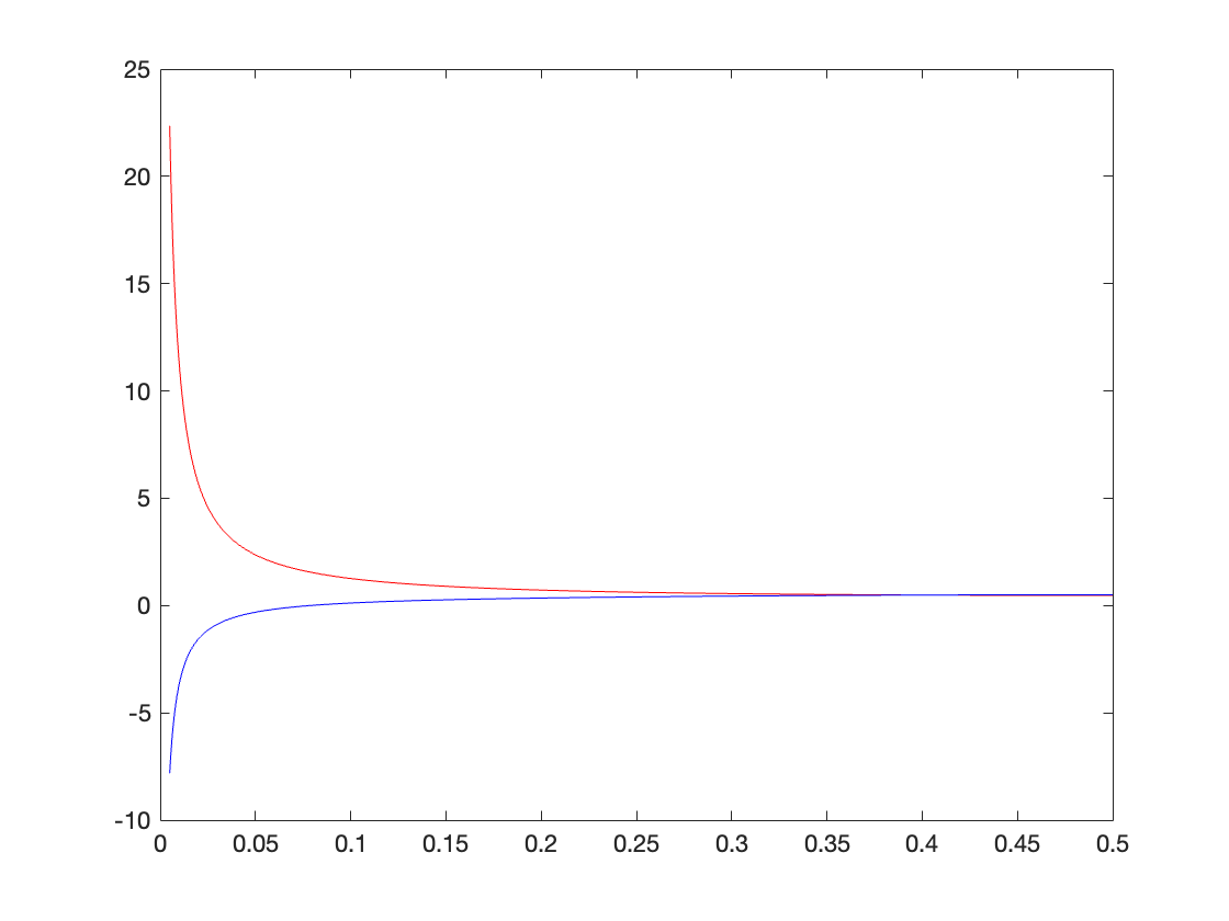
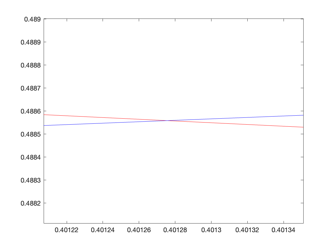
Figure 3: The red lines are graphs of $y=\alpha(x)$ and the blue lines are graphs of $y=\beta(x)$.

References

- [1] Jungho Ahn, Kevin Hendrey, Donggyu Kim, and Sang-il Oum, Bounds for the twin-width of graphs, SIAM J. Discrete Math. 36 (2022), no. 3, 2352–2366. MR 4487903
- [2] Jakub Balabán and Petr Hliněný, Twin-width is linear in the poset width, 16th International Symposium on Parameterized and Exact Computation, LIPIcs. Leibniz Int. Proc. Inform., vol. 214, Schloss Dagstuhl. Leibniz-Zent. Inform., Wadern, 2021, pp. Art. No. 6, 13. MR 4459341
- [3] Natalie Behague, Florian Hoersch, Tom Johnston, Natasha Morrison, JD Nir, Sergey Norin, Pawel Rzazewski, and Mahsa N. Shirazi, 2022, personal communication.
- [4] Édouard Bonnet, Colin Geniet, Eun Jung Kim, Stéphan Thomassé, and Rémi Watrigant, Twin-width III: max independent set, min dominating set, and coloring, 48th International Colloquium on Automata, Languages, and Programming, LIPIcs. Leibniz Int. Proc. Inform., vol. 198, Schloss Dagstuhl. Leibniz-Zent. Inform., Wadern, 2021, pp. Art. No. 35, 20. MR 4288865
- [5] , Twin-width II: small classes, Comb. Theory 2 (2022), no. 2, Paper No. 10, 42. MR 4449818
- [6] Édouard Bonnet, Ugo Giocanti, Patrice Ossona de Mendez, Pierre Simon, Stéphan Thomassé, and Szymon Toruńczyk, Twin-width IV: ordered graphs and matrices, STOC ’22—Proceedings of the 54th Annual ACM SIGACT Symposium on Theory of Computing, ACM, New York, [2022] ©2022, pp. 924–937. MR 4490051
- [7] Édouard Bonnet, Eun Jung Kim, Amadeus Reinald, and Stéphan Thomassé, Twin-width VI: the lens of contraction sequences, Proceedings of the 2022 Annual ACM-SIAM Symposium on Discrete Algorithms (SODA), [Society for Industrial and Applied Mathematics (SIAM)], Philadelphia, PA, 2022, doi:10.1137/1.9781611977073.45, pp. 1036–1056. MR 4415082
- [8] Édouard Bonnet, Eun Jung Kim, Amadeus Reinald, Stéphan Thomassé, and Rémi Watrigant, Twin-width and Polynomial Kernels, Algorithmica 84 (2022), no. 11, 3300–3337. MR 4500778
- [9] Édouard Bonnet, Eun Jung Kim, Stéphan Thomassé, and Rémi Watrigant, Twin-width I: Tractable FO model checking, J. ACM 69 (2022), no. 1, Art. 3, 46. MR 4402362
- [10] Édouard Bonnet, Jaroslav Nešetřil, Patrice Ossona de Mendez, Sebastian Siebertz, and Stéphan Thomassé, Twin-width and permutations, arXiv:2102.06880, 2021.
- [11] Thomas M. Cover and Joy A. Thomas, Elements of information theory, second ed., Wiley-Interscience [John Wiley & Sons], Hoboken, NJ, 2006. MR 2239987
- [12] Reinhard Diestel, Graph theory, fifth ed., Graduate Texts in Mathematics, vol. 173, Springer, Berlin, 2018, Paperback edition of [ MR3644391]. MR 3822066
- [13] Jan Dreier, Jakub Gajarský, Yiting Jiang, Patrice Ossona de Mendez, and Jean-Florent Raymond, Twin-width and generalized coloring numbers, Discrete Math. 345 (2022), no. 3, Paper No. 112746, 8. MR 4349879
- [14] Jakub Gajarský, Michał Pilipczuk, and Szymon Toruńczyk, Stable graphs of bounded twin-width, arXiv:2107.03711, 2021.
- [15] Robert Ganian, Filip Pokrývka, André Schidler, Kirill Simonov, and Stefan Szeider, Weighted model counting with twin-width, 25th International Conference on Theory and Applications of Satisfiability Testing (SAT 2022), LIPIcs. Leibniz Int. Proc. Inform., vol. 236, Schloss Dagstuhl. Leibniz-Zent. Inform., Wadern, 2022, pp. Paper No. 15, 17. MR 4481662
- [16] Wassily Hoeffding, Probability inequalities for sums of bounded random variables, Journal of the American Statistical Association 58 (1963), 13–30. MR 144363
- [17] Choongbum Lee, Joonkyung Lee, and Sang-il Oum, Rank-width of random graphs, J. Graph Theory 70 (2012), no. 3, 339–347. MR 2946080
- [18] Jiří Matoušek and Jaroslav Nešetřil, Invitation to discrete mathematics, second ed., Oxford University Press, Oxford, 2009. MR 2469243
- [19] Michael Mitzenmacher and Eli Upfal, Probability and computing, second ed., Cambridge University Press, Cambridge, 2017, Randomization and probabilistic techniques in algorithms and data analysis. MR 3674428
- [20] Sang-il Oum and Paul Seymour, Approximating clique-width and branch-width, J. Combin. Theory Ser. B 96 (2006), no. 4, 514–528. MR 2232389
- [21] André Schidler and Stefan Szeider, A SAT approach to twin-width, 2022 Proceedings of the Symposium on Algorithm Engineering and Experiments (ALENEX), SIAM, 2022, doi:10.1137/1.9781611977042.6, pp. 67–77.
- [22] Pierre Simon and Szymon Toruńczyk, Ordered graphs of bounded twin-width, arXiv:2102.06881, 2021.