Consistency tests of field level inference with the EFT likelihood
Abstract
Analyzing the clustering of galaxies at the field level in principle promises access to all the cosmological information available. Given this incentive, in this paper we investigate the performance of field-based forward modeling approach to galaxy clustering using the effective field theory (EFT) framework of large-scale structure (LSS). We do so by applying this formalism to a set of consistency and convergence tests on synthetic datasets. We explore the high-dimensional joint posterior of LSS initial conditions by combining Hamiltonian Monte Carlo sampling for the field of initial conditions, and slice sampling for cosmology and model parameters. We adopt the Lagrangian perturbation theory forward model from [1], up to second order, for the forward model of biased tracers. We specifically include model mis-specifications in our synthetic datasets within the EFT framework. We achieve this by generating synthetic data at a higher cutoff scale , which controls which Fourier modes enter the EFT likelihood evaluation, than the cutoff used in the inference. In the presence of model mis-specifications, we find that the EFT framework still allows for robust, unbiased joint inference of a) cosmological parameters — specifically, the scaling amplitude of the initial conditions — b) the initial conditions themselves, and c) the bias and noise parameters. In addition, we show that in the purely linear case, where the posterior is analytically tractable, our samplers fully explore the posterior surface. We also demonstrate convergence in the cases of nonlinear forward models. Our findings serve as a confirmation of the EFT field-based forward model framework developed in [2, 3, 4, 5, 6, 7], and as another step towards field-level cosmological analyses of real galaxy surveys.
1 Introduction
Current and future galaxy surveys such as DESI [8], Euclid [9], PFS [10], and the Vera Rubin Observatory [11] offer a wealth of modes for probing the physics of structure formation. The traditional approach to cosmology inference from galaxy clustering is to compress the galaxy density field into summary statistics, such as two-point (see [12] and references therein), three-point [13, 14, 15, 16], and four-point functions [17, 18, 19].
An alternative approach, and the one we follow in this paper, attempts to extract information at the field level, by explicitly forward modeling the entire observed galaxy density field including all the relevant physics and observational effects. This physical Bayesian forward modeling approach [20, 21, 22, 23, 24, 25] (see also references therein) in principle allows for exploiting information on cosmology beyond -point functions via explicit marginalization over the initial conditions. While the amount of cosmological information available beyond the low-order -point functions is still unclear, this approach, at the very least, allows for a consistent treatment of Baryon Acoustic Oscillation reconstruction [3, 26], and thus is well motivated. Observational systematic effects can be explicitly encoded into the forward model (e.g. [27, 23]), and might be easier to disentangle from cosmological signals at the field level as compared to summary statistics.
So far, the field-level inference approaches have typically used an empirical galaxy bias model and a simplified likelihood to infer from galaxy clustering data. Using dark matter halos in N-body simulations as the reference data, [28] demonstrated that most empirical bias models and likelihoods that have been widely adopted by this approach thus far (e.g. [22, 23]) can significantly bias the inferred cosmological fields. Therefore, the key issue for this approach currently lies in a rigorous physical model, or alternatively, a sufficiently flexible effective model (e.g. [29, 30, 31]) to connect the matter and tracer fields.
The effective field theory of large-scale structure (EFTofLSS) [32, 33, 34] provides a systematic way of incorporating the complex nonlinear physics of galaxy formation on small scales, by using the fact that the galaxy formation is spatially localized and that galaxies and matter comove on large scales (the latter is ensured by the equivalence principle). In particular, the EFTofLSS provides a parametric model for the matter-tracer relation up to the given order in matter density perturbations for any tracer field of interest (see [35] for a review). This, in turn, allows for robust extraction of cosmological information from the tracer data up to quasilinear scales [36, 16], i.e. wavenumbers smaller than the nonlinear scale wavenumber ( at ).
Until recently, the EFT predictions were restricted to summary statistics, but Refs. [2, 5, 4] (see [37] for related work) presented a derivation of a field-level, EFT-based forward model and likelihood. This paper is the next in a series of papers developing this approach [2, 3, 4, 1, 7, 38], with the crucial addition of the marginalization over the initial conditions field by explicitly sampling it. Specifically, we test the consistency of the EFT likelihood – previously demonstrated for fixed initial conditions – on a set of synthetic tracer data and a range of forward models including model mis-specification. The tests of the EFT likelihood approach presented here serve as a crucial stepping stone towards applying the method to more realistic tracers such as dark matter halo or simulated galaxy catalogs. Throughout this paper, we use the following fiducial cosmology: and a box size of . We keep cosmological parameters fixed to the fiducial CDM cosmology but vary a scaling parameter multiplying the initial conditions, which corresponds to varying while keeping all other cosmological parameters fixed.
The structure of the paper is as follows. In Sec. 2, we elaborate on the specific forward models we use for consistency tests of the EFT likelihood. We first describe the simple linear toy models and then physical models based on Lagrangian perturbation theory (LPT), the 1lpt and 2lpt models in Sec. 2.1 and Sec. 2.2, respectively. In Sec. 2.3, we give the description of the EFT likelihoods and the expression for the full field-level posterior being sampled in Sec. 3.1. We outline the sampling methods and the code implementation in Sec. 3.2 and Sec. 3.3, respectively. The synthetic datasets are described in Sec. 4 and the consistency test results are presented in Sec. 5. We conclude and discuss future outlook in Sec. 6. In the appendices, additional details complementing the main results in Sec. 5 are presented and discussed.
2 Forward models
In this section, we present all forward models used throughout the paper (Sec. 2.1 and Sec. 2.2) and we describe the EFT likelihoods, the last piece of our inference framework in Sec. 2.3.
Our forward models aim at modeling the following quantity
| (2.1) |
with representing the number density field of synthetic tracers, its spatial mean, and the fractional overdensity. Throughout this paper, we will work with tracers defined at a fixed time , corresponding to today’s epoch in the fiducial cosmology. Hence, we will drop the time argument for clarity.
We effectively marginalize over by working with and excluding the mode from the analysis. Thus, the field-level forward models consist of two parts: the mean-field prediction , which is a deterministic function of the initial conditions, and the likelihood, constructed from the assumptions about the underlying noise field . We describe the different deterministic forward models used in this paper next, before turning to the likelihoods which couple to all of these deterministic forward models.
The general form of the deterministic contribution is
| (2.2) |
where denote the bias operators and the corresponding coefficients. Depending on the gravity model and the bias model we use, Eq. (2.2) takes on different forms. Since we utilize an EFT approach, our forward models are defined for a specific cutoff . The motivation for this cutoff is twofold:
-
1.
The EFT model developed applies only to large scales. Hence, we want to restrict the likelihood evaluation only to the modes below the cutoff . This in turn means that we need to apply a sharp- cut to the field operators .
- 2.
Throughout, we generate the synthetic data at a higher or equal cutoff than the value used in the inference, motivated by the fact that real-world tracers resemble data with . In fact, real data effectively has no cutoff, i.e. . Below, we describe the specifics of the forward models employed throughout the paper. We focus first on the simplest limiting cases, which involve only linear density fields, and then explain how we build up the 1LPT and 2LPT forward models.
2.1 linear forward models
In linear forward models, the gravity model is restricted to linear evolution, which is incorporated by applying the appropriate transfer function to the initial conditions. On top of this, we also include tracer bias. We consider two different bias expansions. The first one involves only the linear bias and can be expressed as follows
| (2.3) | ||||
| (2.4) |
where denotes a unit Gaussian field which describes the initial conditions (see also discussion in Sec. 3.1), while denotes the transfer function (recall that we keep the time fixed and implicit throughout). Since we keep the cosmological parameters fixed, we do not write them explicitly here. The scaling parameter is defined such that, for , corresponds to a realization of the linear density field in the fiducial cosmology. denotes the isotropic sharp- filter111See App. A for more details and our Fourier space convention. at . For this forward model (Eq. (2.3)), it is possible to analytically derive the posterior for the initial conditions (see App. B.1 for detailed calculation), and hence to test whether our inference approach fully explores the posterior in this case.
The simplest extension of the above forward model is to include also the quadratic field with the corresponding bias parameter:
| (2.5) |
with given by Eq. (2.3). The bias expansion here is not complete in the EFT sense; we employ this forward model merely as the simplest possible generalization from an entirely linear forward model. The complete second-order bias expansion is considered in the next section. Nevertheless, due to the nonlinearity induced by the quadratic bias, the posterior is non-Gaussian and it is non-trivial to make exact statements about its statistical moments (see App. C for further discussion). The models given by Eqs. (2.3)–(2.5) thus serve as toy models for which there exists full or approximate analytical expression of the posterior. They both assume all the relevant information is contained within the linear density field and do not involve nontrivial gravitational displacements, which are however essential when attempting field-level inference on real data.
2.2 1LPT and 2LPT forward models
The forward models in Eqs. (2.3)–(2.5) are valid only for describing tracers at linear order. In order to obtain more accurate descriptions at higher orders – which properly account for gravitational evolution – we turn to Lagrangian perturbation theory. The Lagrangian formulation of structure formation captures the effect of bulk flows non-perturbatively. This is especially useful for forward modeling. To be more precise, we consider a first- and second-order LPT, labeling them with 1LPT and 2LPT, respectively.
We begin by writing the Eulerian position along the fluid line at conformal time as
| (2.6) |
with being the Lagrangian coordinate, the displacement field and . We also re-instate the explicit dependence throughout this overview for clarity. Combining the mass conservation condition and the Poisson equation for the non-relativistic (cold) dark matter fluid yields the following equation of motion for [39, 40, 41, 1]
| (2.7) |
where is the symmetric part of the Lagrangian distortion tensor, the primes denote derivatives with respect to , is the corresponding matter density parameter and the conformal Hubble rate. We restrict to the symmetric part of throughout, since the antisymmetric part, corresponding to the curl of , is only nonzero at third order in perturbations and here we restrict ourselves to second order. Thus, is a longitudinal vector and can be written as
| (2.8) |
Lagrangian perturbation theory then proceeds by expanding [42]
| (2.9) |
and analogously for and , where involves exactly powers of the linear density field . In fact, . For a given expansion history, Eq. (2.7) can be formally integrated to yield recurrence relations relating to the lower-order contributions [39, 40, 41].
The perturbative contributions to in Eq. (2.9) can serve as building blocks for a general bias expansion of the form given in Eq. (2.2). The reason is that the Lagrangian distortion tensor along the fluid trajectory captures all leading gravitational observables for a comoving observer (see section 2.5 in [35] and [43]). Specifically, one needs to construct all scalar contractions of the , , that are relevant at the given order . At second order, this yields
| (2.10) |
where we emphasize that is in Lagrangian coordinates. Thus, up to second order, we require three distinct bias operators and the associated bias coefficients.
In order to obtain the corresponding Eulerian fields we use a weighted particle approach [37, 1]. We consider pseudo particles on a regular grid in , and assign each of them 3 weights corresponding to the three bias operators. Then, each of these pseudo particles is displaced from to , and the masses are deposited to the grid using a mass-conserving assignment scheme (we choose cloud-in-cell assignment here). This yields the three Eulerian operators corresponding to the Lagrangian operators listed above. In fact, we replace the weight field with a unit weight field, so that the resulting Eulerian field is the LPT matter density field (), and use this linear bias term in Eulerian frame.
Finally, we also include the leading-order higher-derivative bias contribution (see sec 2.6 in [35]), , computed in the Eulerian frame, in order to capture the finite spatial size of the regions forming the tracer of interest. Therefore, the full list of bias parameters and corresponding operators is
| (2.11) |
where we emphasize the presence of the cutoff . The linear displacement tensor is related to the linear density perturbation via
where is defined in Eq. (2.4).
2.3 Field-level likelihood
Instead of modeling directly the tracer number counts, as done for example in [22, 20], the EFT likelihood aims to describe the tracer density field . It is obtained by integrating out the modes with in the initial conditions [5]. These small-scale modes also produce a stochastic contribution to the predicted galaxy density field . This effect is encoded by the noise field, . Since this effective noise field arises from the superposition of many independent modes, it is Gaussian to leading order. Moreover, because the tracer formation is spatially local, the power spectrum of the noise is constant to leading order, with corrections scaling as [35]. In other words,
| (2.12) |
where denotes the Dirac delta function, and we have denoted with the leading order contribution to the noise covariance. Note that the scale-dependent correction, , is written here as fractional correction by convention. In general, the gravitational evolution of small-scale modes under the influence of large-scale modes generates density-dependent noise terms, which cause the noise covariance to be non-diagonal in Fourier space. We do not consider these contributions here, since all synthetic datasets used here do not contain such density-dependent noise. The exception is the 2LPT synthetic dataset (see Tab. 1). In this case, the second-order bias coupled with the presence of a cutoff mismatch between synthetic data and inference forward models can generate density-dependent noise. We also set the subleading noise contribution to zero throughout this paper. More detailed investigations of the impact of the noise model are relegated to future work.
Our data model is then given by
| (2.13) |
where is given by one of the forward models we consider here, namely Eqs. (2.3)–(2.5) or Eq. (2.11). In the second line of 2.13 we emphasize that the noise field is assumed to be Gaussian distributed with covariance structure given by the leading term from Eq. (2.12). Specifically, the noise variance on the real-space grid of size and box size is defined through the following relation
| (2.14) |
In this paper, we consider two forms of EFT likelihoods: one whose arguments explicitly include bias parameters, hence labeled unmarginalized likelihood, and the other one where bias parameters are analytically marginalized out, the marginalized likelihood. Below we detail the two likelihoods in that order. The notation closely follows that in [3]. We also switch to the discrete Fourier space representation of the fields (see App. A for details on our Fourier space convention).
From our assumption of Gaussian noise it follows directly that the likelihood is likewise Gaussian. Namely,
| (2.15) |
where we have explicitly stated the dependence of on bias parameters, , the scaling parameter and the initial conditions . Note that is a deterministic function of these parameters and that the likelihood is evaluated only up to , strictly allowing only for modes below the cutoff. In order to maximize the information gain, we choose . We accumulate all the terms which depend neither on , , nor in const., since they represent only irrelevant normalizing factors.
The marginalized likelihood is obtained by analytically marginalizing over all bias parameters in Eq. (2.15). Given that the likelihood depends quadratically on any bias coefficient (in case priors on the bias parameters are Gaussian or uniform on ), this is a straightforward calculation (see section 2.2 in [3]). The expression is
| (2.16) |
where, once again, const. encapsulates the terms independent of the parameters of interest. The marginalization was performed under the assumption of a Gaussian prior on bias parameters with covariance and mean . We choose a fairly uninformative prior as given in Eq. (3.3). As indicated, the information on and the initial conditions is propagated through the and operators.
3 Sampling the full posterior
Here, we provide the final expression for the posterior being sampled and elaborate more on some specific choices of our sampling scheme, as well as some additional details of our code implementation.
3.1 Full posterior
The results of the previous section now allow us to write the full posterior which we aim to sample from. The expression can be obtained readily from
| (3.1) |
where represents the posterior probability of the parameters of interest given the synthetic data, the corresponding likelihood (see Eqs. (2.15)–(2.16)), while represents the associated prior. The represents the evidence, which does not play any role in our inference framework. As noted in Sec. 1, we keep all other cosmological parameters fixed to the fiducial values listed there.
We assume minimal prior knowledge on and the . Moreover, as physical parameters describing the properties of the tracers, they are a priori independent of the initial conditions . Therefore, the joint prior structure is entirely factorized. We choose the following prior configuration throughout the paper for the unmarginalized likelihood:
| (3.2) |
where denotes the uniform distribution on interval . Note that here we choose to keep the prior on strictly positive, as we do not consider the modeling of negative bias tracers, such as voids, within this paper. We chose priors of the higher-order bias coefficients to be symmetric around zero, as a priori these bias coefficients could take on either sign.
For the inference with the marginalized likelihood, the only difference is in the priors for the bias parameters, which are taken to be of the following form
| (3.3) |
Given the signal-to-noise level of our synthetic datasets, these priors are essentially uninformative, and we expect an entirely negligible difference in parameter inferences between marginalized and unmarginalized likelihoods.
Finally, for the prior on the initial conditions, we consider the following two choices:
| (3.4) |
where we have separated the cases with fixed initial conditions to the ground-truth (fixedIC) and with initial conditions explicitly sampled (freeIC). In the latter case, the prior covariance structure of the discretized field is given by , while in Fourier space it becomes , with being the grid size corresponding to the cutoff , and denoting the Kronecker delta (see App. A for details on our Fourier convention).
The fixedIC case corresponds to that considered in the application to dark matter halo catalogs in previous papers of this series [2, 3, 4, 1, 7], where the parameter was shown. Moreover, the same setup was used to measure bias parameters of simulated halos and galaxies in [44, 45]. For real-data applications, as we have no knowledge of the true initial conditions a priori, it is crucial for our method to properly marginalize over all plausible realizations of the initial conditions. Thus, the parameter posterior obtained on our synthetic datasets with the fixedIC prior serves as a good reference point for the freeIC case. Specifically, we expect consistency between the fixedIC and freeIC posterior parameter means, which we demonstrate in Sec. 5.
3.2 Sampling methods
In order to explore the posterior surface of the parameters of our model, we utilize a combination of slice sampling (see Sec. 29.7 in [46] and [47]) and Hamiltonian Monte Carlo (HMC) sampling techniques (see [48, 49] and Sec. 30.1 in [46]). Below, we motivate this choice of sampling techniques, which was inspired by the findings made in the development of the borg code (see, e.g. [22]).
The slice sampling technique is used for sampling , bias parameters , and the noise parameter . This means that we actually sample the 1D probability density function of these parameters conditioned on the current realization of initial conditions . We adopt sequential univariate slice sampling, i.e. we sequentially sample individual parameters. While multivariate slice sampling methods do exist, they require additional tuning to be more efficient than our approach (see the discussion in section 5 of [47]).
When it comes to sampling the posterior of the initial conditions , we use the HMC sampling technique. The reason behind this choice is that the number of Monte Carlo samples needed for generating an independent sample scales more efficiently with the problem dimensionality than for standard Monte Carlo methods. This scaling goes as in the case of a standard random-walk algorithm, while it goes as for the HMC method (see, for example, Sec. 4.4 of [49]). For the problem we consider here, typically . Therefore, HMC currently appears to be the most (if not only) practical sampling method to tackle such a problem.
In order to utilize HMC, one needs a fully differentiable forward model with respect to the initial conditions. This requirement is necessary for the crucial step of generating a new proposal of initial conditions, consistent with the data likelihood. This new proposal is generated by numerically integrating along the Hamiltonian flow defined by the likelihood and prior gradients with respect to the initial conditions . For this, we choose the second-order leapfrog integrator, although see, e.g. [50, 51], for the applicability of higher-order integration schemes.
Given the structure of our code, LEFTfield222Lagrangian, Effective-Field-Theory-based forward model of cosmological density fields., described in Sec. 3.3, the analytical derivative of the full forward model can be readily obtained through successive applications of the chain rule.
Finally, readers may ask why not try to combine the two sampling approaches such that all the parameters are sampled within the HMC scheme at the same time. This however is unfeasible, due to the large difference between the derivative norms of the variation with respect to and the variation of the rest of the model parameters. Variation of or bias parameters affects all the modes of the forward model, while the derivative with respect to a given only has to vary a single mode at a time. This in turn requires the HMC trajectories to be integrated with small step sizes, in order to reach a reasonable acceptance rate, and ultimately results in a very slow exploration of the (joint) posterior surface.
Therefore, decoupling the sampling of , bias, and noise parameters from the sampling of initial conditions seems to provide the fastest exploration time. Note that, in such a block-sampling scheme one could still use the HMC method to sample cosmological and bias parameters, conditioned on a given realization of the initial conditions. One could separate the former and latter into two separate HMC sampling blocks with two different equations of motion (to be integrated). However, since the dimension of the cosmological and bias parameter space is currently negligible, we opt for the robustness of slice sampling.
3.3 Code implementation
The forward models and likelihoods described in Sec. 2 are implemented in the differentiable code LEFTfield. LEFTfield adopts the C++17 standard and represents a substantially extended and more efficient version of the code presented in [1]. Most importantly, LEFTfield implements the gradient of the likelihood with respect to the initial conditions , which as noted is crucial for the HMC sampling approach. A public release of the code, subject to additional tests and tidying up, is planned for the future.
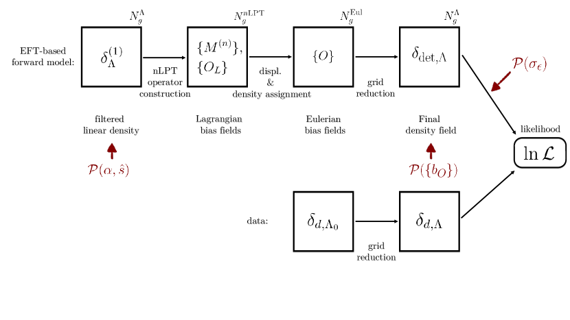
The code is structured in a modular way, breaking down the forward model into a series of simple steps, called “forward elements”, which are templatized on generic input and output types and implement the general behavior of composed operator chains; specifically, the respective input and output types need to match for all composed forward elements. The sequence of high-level operations contained in the forward models are represented in the top row of Fig. 1 (note that each of the blocks, in general, consists of multiple forward elements). The forward model starts from a sample of initial conditions from which one obtains the initial density field , shown in top left of Fig. 1. The size of this grid is chosen based on the cutoff . This is indicated with . The next element is the bias operator construction. For this, we use the set of bias operators appearing in Eq. (2.10) in the case of 1LPT and 2LPT models. At this step, care is also taken for representing all the physical modes of the forward model, by choosing appropriate grid sizes, indicated with . Afterward, these fields are displaced utilizing a weighted particle scheme to the final Eulerian positions. This results in a mapping , where now the operators are assigned onto a grid of size , chosen in advance, with in order to keep all physical modes of the forward model represented on the Eulerian grid. In the end, the set of the displaced bias operators is resized in Fourier space to a smaller and final grid corresponding to , using the sharp- cutoff. Finally, the deterministic prediction from Eq. (2.11) is constructed in the last piece of the top row. This also involves drawing a new set of relevant bias parameters from the corresponding prior. The grid reduction and grid padding are both performed in Fourier space. Several options for mass assignment schemes are implemented, including nearest-grid-point (NGP, which is not differentiable however), cloud-in-cell (CIC), and triangular-shaped cloud (TSC). In this paper, we use the CIC scheme throughout. The very last piece of the forward model is the evaluation of the likelihood, given by either Eq. (2.15) or Eq. (2.16). Note that the forward models of Sec. 2.1 are much simpler, but have the same overall structure.
In the case of the HMC sampling block, the full gradient of the likelihood with respect to the initial conditions, , needs to be evaluated. In order to do so, we utilize the chain rule, collecting every -dependent term of each element in the forward model, from right to left in the flowchart. In addition, for every sample of , the slice sampler generates a new sample of the other parameters of interest. This process is repeated until the desired number of samples is achieved (see Sec. 5 and App. D for more details on our convergence requirements and verification).
The bulk of the computing time is spent in the HMC sampling of the initial conditions. For reference, we provide some benchmark computing times here. For the 2LPT forward model with grid size, LEFTfield generates samples per CPU hour, roughly corresponding to effective sample per CPU hour, running on a single Intel(R) Xeon(R) Gold 6138 CPU @ 2.00GHz with 20 cores and using OpenMP parallelization.
4 Synthetic datasets
In this section, we describe how precisely we generate the synthetic data sets (the first element in the bottom row of Fig. 1). In general, a dataset is generated from each of the aforementioned forward models. We introduce model mis-specification through the mismatch between the cutoff in the synthetic data and a varying cutoff in our forward models, as indicated in the two elements in the bottom row of Fig. 1. We always fix . Throughout, we label the specific realization of initial conditions used for synthetic data generation by . All parameters of the synthetic datasets are summarized in Tab. 1.
4.1 linear model synthetic data
| Dataset \ Parameter | ||||||||
|---|---|---|---|---|---|---|---|---|
For the models described in Eqs. (2.3)–(2.5) we generate two sets of synthetic data: one with and the other with . Below, we specify the parameter values adopted and explain our choice.
The first case of synthetic data, , is obtained with the parameters listed in the first row of Tab. 1. Note that the cutoff set by determines the grid size, which in this case is . This grid size most closely corresponds to the Nyquist frequency for the cutoff and a box size . The parameter is the square root of the noise variance on this grid, which corresponds to a Poisson shot-noise for tracers with comoving number density of . Since the noise power spectrum is a physical quantity (in particular, independent of the grid size), it follows from Eq. (2.14) that the combination must be independent of the grid size corresponding to the cutoff . This implies that itself depends on the grid size . Therefore, instead of working with , we define the following quantity
| (4.1) |
which is grid-size-independent by construction. The prefactor is introduced for numerical convenience. We will mainly quote instead of in our posterior analyses in Sec. 5. As can be seen from Tab. 1, we adopt a comparable noise level for all synthetic datasets except for , which we describe below.
The second synthetic dataset, comes in two variants, listed in the second and third row of Tab. 1. We always choose in order to introduce a non-negligible mode coupling through the quadratic term in Eq. (2.5). In addition, we consider (third row of Tab. 1), using a very low noise level () and hence representing a very informative dataset. This dataset was included to further investigate the dependence of the inferred as a function of the cutoff (see Sec. 5.1.2).
Apart from the case of , for all other datasets, including datasets, we generate two different data realizations. We achieve this by generating two different initial conditions realizations, keeping the values for the remaining parameters fixed. Independent inferences are performed on both data realizations. This helps us gauge the significance of any mis-estimation of the posterior and hence of potential systematic trends in the inferred parameters. Henceforth, we label the different data realizations by the subscript , for example and which correspond to the two different realizations of the synthetic dataset listed in the second row of Tab. 1.
4.2 2LPT synthetic data
We generate two types of synthetic datasets for the 2LPT forward model described in Eq. (2.11). They are labelled as and and their parameters are listed in the last two rows of Tab. 1. As before, we also generate two different realizations of each of these datasets.
The datasets serve as an input for the internal consistency between the 2LPT and 1LPT forward models. In particular, these correspond to a noisy, but unbiased tracer of the matter field itself, given that with all higher-order bias coefficients set to zero. We demonstrate in Sec. 5.2.1 that we exactly recover the fiducial values of parameters in case of 2LPT and that we also recover the expected shifts of parameters in the case of the 1LPT forward model. We calculate these shifts analytically in App. E.
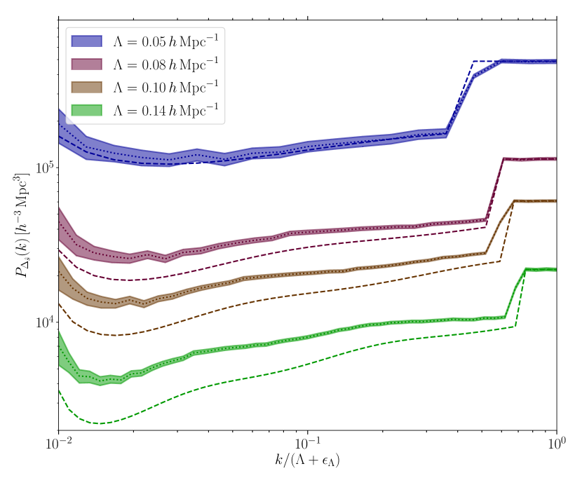
Finally, the datasets contain nonzero higher-order bias coefficients. These are the most realistic datasets considered here, in the sense that they contain complications due to both nonlinear gravity and nonlinear bias. Since the calculation of the running of the bias parameters with cutoff is substantially more involved in this case, we instead validate our field-level forward model based on the inference of the parameter for this case. If the EFT likelihood is able to correctly absorb the effect of modes above the cutoff, then it should lead to an unbiased inference of for all values of .
5 Consistency test results
In this section, we describe the analysis procedure of our MCMC chains. Since the dimensionality of our posterior is exceptionally high, fully characterizing it is challenging [52], even with HMC sampling. To ensure that our samples fairly represent the true posteriors, we strictly adopt the following setup and procedure:
-
•
We run MCMC chains with both free initial conditions (freeIC) and initial conditions fixed to the ground truth (fixedIC). Since it is expected that the posterior of the fixedIC case is within the typical set of the freeIC posterior, in case of no strong multi-modality, it serves as a good reference point. Indeed, we find a good agreement between the joint posteriors of these two cases (see also the next bullet point), suggesting no strong multi-modality is present in the tests we consider in this paper.
-
•
For freeIC runs, we run at least three chains: two starting from randomized values of initial conditions and sampled parameters, and one more chain starting from the ground-truth. The latter serves as an additional check on multimodality of the posterior, and of the convergence of our chains.The remaining parameters differ among the forward models we consider here and we always indicate which parameters are actually sampled.
-
•
In our analysis, we discard the initial part of each chain, which is typically correlation lengths long (see App. D on how we obtain the correlation lengths). Throughout, for each reported inference, if we run more than one MCMC chain as described in the previous point, we combine the chains into one single set of posterior contours. The consistency between different chains being combined is verified with the Gelman-Rubin statistics described in the next point.
-
•
We evaluate the Gelman-Rubin statistics [53, 54, 55] for our MCMC chains as described in App. D. In doing so, we also quantify the (combined) effective sample size. The results for both the Gelman-Rubin statistics and the effective sample size, for all our chains, are listed in Tab. 2, 3 and 4. We require all of our chains to have effective samples. This allows us to have the MCMC sampling error reduced to , which is sufficient for the purposes of this paper.
It is also important to note that for the freeIC chains, we use different -binned quantities in order to check their statistics and convergence. These are the power spectrum of , the mean deviation from and the corresponding power spectrum of this deviation. Additionally, we have verified that the convergence of individual modes is well represented by the -binned quantities for the different bins. We also note that both the -binned quantities and the individual modes converge much faster than other parameters of the model, namely , and .
We will also compare the sampled posterior with analytical predictions. For the latter, we always first calculate the per--mode prediction, and then compute the -bin average, which is then compared with the corresponding sampled posterior in the same -bin.
5.1 linear forward models
5.1.1 Linear bias
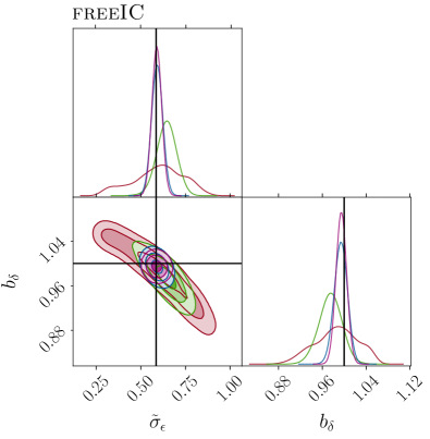
First, we discuss the results of the forward model with linear bias expansion. In this case, it is possible to calculate the posterior of the initial conditions analytically. The comparison with the sampled posterior then verifies whether our sampling approach indeed fully explores the posterior in this case. As a first result, we focus on Fig. 2. In this figure, we show the projection of the posterior to the plane. We distinguish two cases. The case where the posterior contours were obtained by fully marginalizing over the initial conditions (freeIC), shown in the left panel, and the case where the initial conditions were fixed to the ground-truth (fixedIC), shown in the right panel. The two panels indicate that the freeIC and fixedIC posterior means are consistent. Note the stark contrast in the posterior widths between the fixedIC and freeIC cases. This is explained by the fact that, in the case of fixedIC, only two parameters need to be constrained, while in the case of freeIC the joint posterior simultaneously constrains degrees of freedom. More specifically, the free initial conditions also allow for an overall change in the amplitude, leading to the wider posteriors in . We also observe that the posterior contours shrink with increasing , as expected. The degeneracy between the amplitudes of the signal () and noise () is harder to break at lower due to the shallower slope of the linear power spectrum, hence resulting in posterior uncertainties that grow faster toward smaller than expected merely from mode counting arguments; i.e., the error bar on grows toward smaller more rapidly than . The stronger degeneracy in the plane also results in a slower exploration by the samplers, evidenced by a longer correlation length, which we do not explicitly show here for conciseness.
Another point to emphasize is that the correct fiducial noise level has also been recovered at in all cases. This means that our inferences clearly disentangle between the actual signal and Gaussian noise contributions. We emphasize that the contour lines in 2D posteriors always indicate in that order, which corresponds to the , and levels respectively.
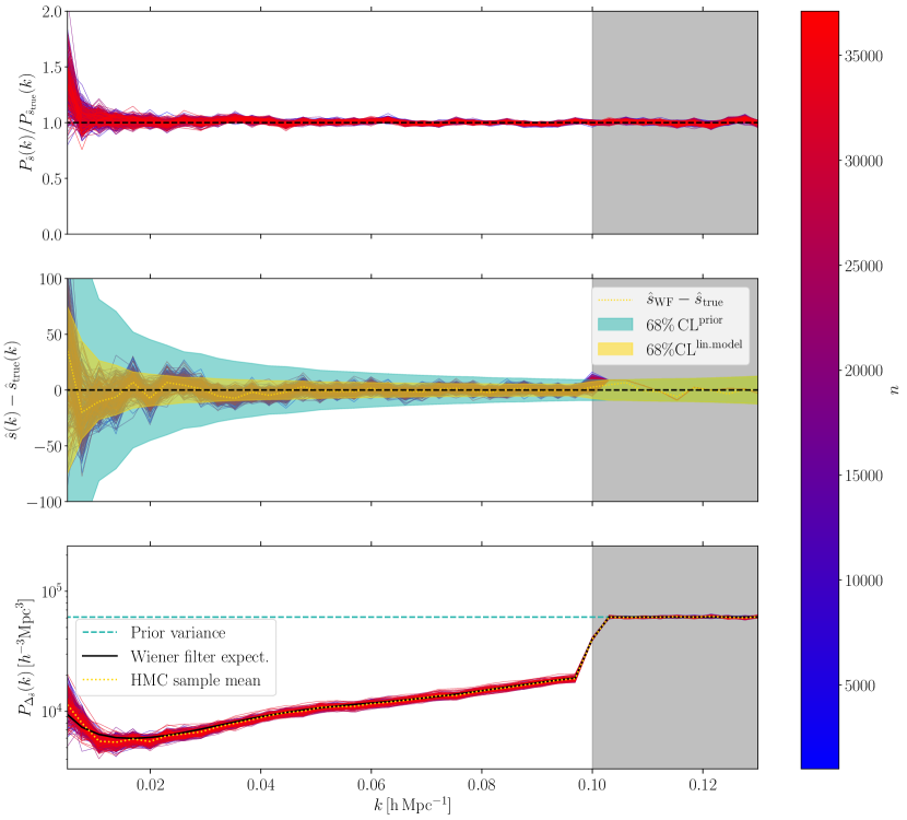
We now turn to investigating the posterior of the initial conditions , focusing in particular on whether the inference is able to recover the true initial conditions used in generating the synthetic data, . Fig. 3 compares the bin averaged quantities of the inferred and true initial conditions as a function of Fourier wave number . The inference was performed on the dataset, at the cutoff of , keeping the other model parameters free. The top panel of Fig. 3 shows the ratio between the power spectrum of and that of . The ratio is consistent with unity, indicating that the two fields agree in terms of power, or mean amplitude.
The middle panel of Fig. 3 depicts the -bin averaged statistics of the residuals . Indeed, their distribution is centered around 0, clearly implying that the bulk of the posterior closely traces the field.
Note that we do not expect the posterior to be always centered around the field, but that is within the typical set. We can in fact be more precise. As we show in App. B.1, the posterior mean and covariance for the linear model considered here is, in the case when the parameters and are fixed to their fiducial values, given by
| (5.1) |
with
| (5.2) |
and the reduced density field of the synthetic dataset. As seen from Eq. (5.1), the posterior exhibits two limits. First, in the limit of uninformative data, i.e. large noise , the posterior approaches to the prior, and the posterior mean of approaches zero while . Second, in the limit of very informative data, i.e. small noise , the posterior mean and covariance approach , following Eq. (2.3), and , respectively.
The yellow dotted line in the middle panel of Fig. 3 represents the residual between the Wiener-filter solution , i.e. the linear model analytical prediction from above, and . Clearly, the sampled posterior is precisely centered around , indicating that it is unbiased also in the case when and are left free. Above the cutoff, indicated by the gray band, the sampled modes follow the prior, hence . However, due to the finite number of modes per -bin, the calculated mean will not be zero exactly but vary around it within the prior bounds, which is indeed what we see.
Finally, the bottom panel of Fig. 3 shows the power spectrum of the field. The theoretical expectation is that the power spectrum of in a given -bin is distributed, , where the shape parameter is , being the number of modes within the Fourier space shell centered on , and the scale parameter is . This conclusion follows from considering the distribution of a sum of squares of Gaussian-distributed variables, in this case, . Since the mean of the distribution is given by the product of its scale and shape parameter, it follows immediately that the expectation value of within a given -bin is .
This prediction is shown as the black line in the bottom panel of Fig. 3. We find good agreement with the sampled results, indicating that the posterior is fully explored by the sampler. We expect this to be the case, even though the Wiener filter calculation assumes fixed parameters. Given that and parameters are very well constrained, the propagated effect of their variance is a subdominant contribution to the posterior variance. We also show the prior covariance for comparison, and as we can see, modes above the cutoff indeed follow the prior.
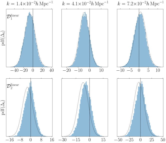
To further investigate the posterior, in Fig. 4, we plot, for three selected -bins, both the histogram of and the corresponding Wiener filter prediction, . The latter is, of course, Gaussian and plotted as the dotted line. To guide the eyes, we also show a vertical line on zero, indicating the ground truth. The top panel of this figure depicts the inferred residual statistics of the linear forward model from Eq. (2.3). In this case, the predicted (Wiener-filter) and sampled posteriors fully agree. On the other hand, the bottom panel shows the same, but for the forward model including second-order bias (Eq. (2.5)). Here we see clear deviations between the analytical and sampled posteriors. The posterior for this simple but nonlinear forward model is not well approximated by the Wiener-filter solution (see Sec. 5.1.2 and App. B.2 for more details). This highlights the importance of going beyond the Wiener filter approach when trying to extract information from even mildly nonlinear scales.
5.1.2 Second-order bias
Next, we perform consistency tests of the EFT likelihood on the datasets. These synthetic datasets are generated using the forward model in Eq. (2.5). They additionally include a non-negligible quadratic bias contribution. Note that this contribution however still involves only the linearly evolved density field . This results in a non-Gaussian posterior of the initial conditions, , about which nonetheless we are able to make some qualitative analytical statements (see App. B.2 and App. C).
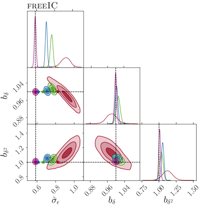
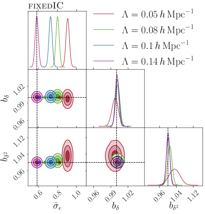
First, we analyze the posterior of the inferred parameters shown in Fig. 5. As before, we consider forward models with different cutoffs . Here, since the synthetic data is generated with a nonzero , it introduces mode couplings across the whole available range of modes up to the synthetic data cutoff of .
We first look at the noise amplitude . Fig. 5 shows that the inferred value is a function of the cutoff for both fixedIC and freeIC cases; the inferred value is largest for the forward model with and lowest for . This can be understood as follows. The synthetic dataset is generated using the forward model from Eq. (2.5), but with a cutoff of (see also Tab. 1). We can then split the linear density field from which the synthetic dataset is constructed as
| (5.3) |
where and represent the parts of containing modes up to , and from to , respectively. Thus, contains a contribution (see Eq. (2.5)). Since is uncorrelated with , this contribution to the data corresponds to an additional noise that is absorbed in during the inference. We thus expect to shift by the power spectrum of , leading to
| (5.4) | ||||
and is the linear power spectrum. Notice that only Fourier modes in the shell contribute. Evaluating this at leads to the results represented with stars in Fig. 5. Note that for the case of (purple), there is no running of parameter and the corresponding star is right in the center of the posterior contours for this case. In general, we find that the analytical result predicts the right trend, although the shift in the sampled posterior mean is generally larger than the prediction, in particular for values that approach . The most likely explanation is that the inferred also has to absorb the scale-dependence of the induced noise, since Eq. (5.4) has a significant -dependence in particular if is not much smaller than .
We now turn to the bias parameters. First, we expect no running of with the cutoff , as the former only multiplies the linear density in the forward model Eq. (2.5). In other words, for all . In fact, this argument can be made rigorous by examining the maximum likelihood point of the EFT likelihood (see for example Sec. 4 of [2]). Note that the maximum likelihood argument assumes the initial conditions fixed to the ground truth . Strictly speaking, the argument applies only to the fixedIC case. However, we generally expect the freeIC posterior to overlap the fixedIC one, and Fig. 5 confirms that this is indeed the case.
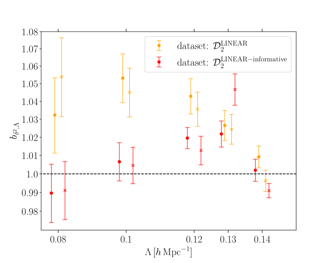
We derive the running of the parameter with the cutoff in App. C and show that it vanishes as well; i.e., . We plot the results for for the different freeIC chains in Fig. 6. There is a residual shift away from the expected value of when considering synthetic datasets with , as shown by the yellow data points. While we expect the model from Eq. (2.5) to be more accurate toward lower , we in fact observe that the shift in with respect to the expected result increases as we lower the cutoff. The most plausible explanation for this is a prior volume effect resulting from the weakening constraint on and the growing degeneracy with toward lower (see Fig. 5). To confirm this, we performed an inference with substantially lower noise (), indicated by the red points in Fig. 6. Indeed, the systematic shift is substantially reduced, showing that more informative datasets help with breaking the degeneracy.
To conclude, the expected values for the bias parameters are precisely recovered at to levels by our freeIC posteriors. The only stronger deviation occurs for forward models with cutoffs , which persists even in the case of highly informative data (see Fig. 6). It is possible that including the subleading, contribution to the noise, which is expected to become more important as approaches , would help with this residual shift.
Next, we focus on analyzing the posterior. As before, we look at the first and second moments of the posterior of initial conditions. However, now the Wiener filter prediction for the posterior mean is less accurate than for the case shown in Fig. 3 due to the presence of the quadratic term in the forward model. Fig. 7 compares the estimated from the chain samples (dotted lines, with bands indicating sample variance) with the Wiener-filter expectation for the variance (dashed lines). As expected, the deviation from the Wiener-filter solution is stronger, at fixed , as we go toward higher cutoffs. This is both because the typical amplitude of density fluctuations grows on smaller scales, and the uncertainty on shrinks.
We can in fact make some qualitative statements about the behavior seen in Fig. 7. In the case of the quadratic bias forward model, the posterior of initial conditions contains terms proportional to and , in addition to the terms and present in the purely linear case. The posterior covariance depends on all of these terms, as demonstrated in App. B.2. There, we consider under what conditions the posterior for can be approximated analytically and describe the cause for the discrepancy between the Wiener filter prediction and the sampled joint posterior.
5.2 1LPT and 2LPT forward models
We now turn toward the forward models involving nonlinear gravity, i.e. 1LPT and 2LPT. The forward models we consider in this section are the most realistic ones, and allow for reducing the degeneracy between the bias parameters and the scaling parameter, , as we elaborate below. Furthermore, as already hinted in [2], these forward models promise information gains beyond the leading-, next-to-leading order power spectrum, and leading-order bispectrum. We leave it for future work to explicitly demonstrate this. Instead, below we focus on the performance of these forward models on synthetic datasets listed in Sec. 4.2.
5.2.1 Linearly biased case
The synthetic dataset used in this section is , with different realizations denoted by and . These correspond to a linearly biased tracer of the 2LPT-evolved matter density field, and we thus test the consequences of a mismatch in the nonlinear matter forward model. For the forward models considered here, the exact degeneracy between and that is present for trivial linear evolution is broken, as contains terms scaling as and both multiplied by the same (see [3, 4] for more discussion).
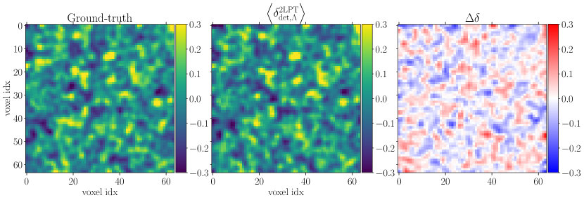
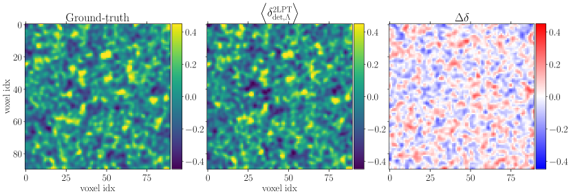
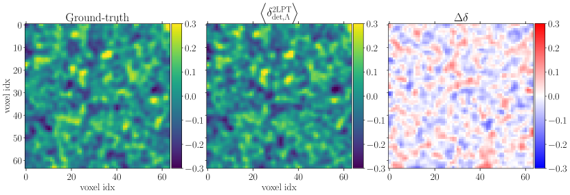
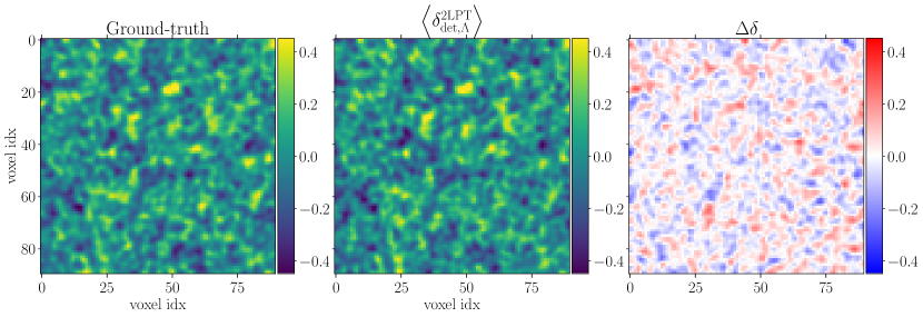
In Fig. 10 we show how well the posterior mean of the inferred field in the freeIC case with randomized initial conditions taken as the starting point compares to the ground-truth signal used for generating the dataset. We show results for both cutoffs considered: (upper panel of the figure) and (lower panel of the figure). For obtaining the posterior mean of , the last samples of the inference chain were taken. The final results were additionally smoothed with a Gaussian kernel of size along each axis, for aesthetic reasons. Overall, the reconstructed field in the selected slice matches well the ground-truth signal. In the regions with highest density peaks, the residuals are quite small as expected, however due to the stochastic nature of our forward model, the reconstructed and ground-truth field don’t match exactly. Once more we emphasize that this result has been obtained by joint sampling of the initial conditions, and bias parameters as well as the noise parameter , and therefore represents a non-trivial result. We focus on the parameter posteriors next.
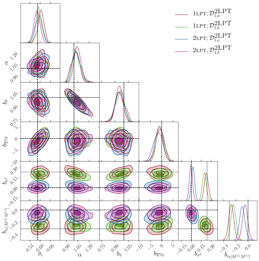
Fig. 11 shows the parameter posteriors after explicitly marginalizing over the posterior of initial conditions. Here we compare the inferences employing the 1LPT (red and green contours) and 2LPT (blue and dark-purple contours) forward models. The parameters , , and , which are not expected to run, agree well among the two different gravity models. The running is not present since is a cosmological parameter, while and are protected from running thanks to the absence of nonlinear bias in the synthetic datasets . Note however that is expected to absorb the effect of modes between and , hence to be shifted from its fiducial value. We also observe an expected anti-correlation in the plane, given that these two parameters appear together as a product in the linear bias term in the forward model.
Another interesting degeneracy is in the plane, which shows positive correlation. This can be understood by recalling how these parameters affect the leading order observable, the power spectrum. The dominant contribution to the tracer power spectrum that contains is at , while the noise contribution scales as . Since these two contributions have a similar dependence, but opposite signs, they result into a positive correlation between the two corresponding parameters.
We also notice the difference between the 1LPT and 2LPT posteriors in the bottom two rows of Fig. 11. Namely, the higher-order bias coefficients inferred using the 1LPT forward model are shifted away from their fiducial values of zero. The shifts of these bias coefficients can in fact be predicted using a second-order LPT calculation. Specifically, by solving for the displacement field and then substituting that back into the second-order bias expansion, one can derive the relations between the bias coefficients in the 1LPT and 2LPT forward model. Following the calculation done in App. E, one derives the following relations between the bias coefficients of the two forward models
| (5.5) |
These values are indicated with dotted lines in Fig. 11, and are within of the corresponding 1LPT posteriors.
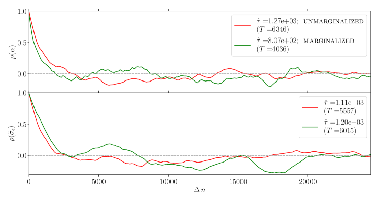
The results we have discussed so far were obtained using the likelihood from Eq. (2.15), i.e. the unmarginalized likelihood. Using the marginalized likelihood from Eq. (2.16) gives entirely consistent results (see App. F). However, the marginalized likelihood offers the important advantage of a reduced correlation length in the remaining parameters . Namely, marginalizing over the bias parameters allows for a reduction in the correlation length of the parameter (see the top panel of Fig. 12).333Note that the correlation length was estimated by taking the average over three (two) independent chains for the unmarginalized (marginalized) likelihoods, respectively.
This in turn means that for the same CPU time, the number of effective samples produced by the marginalized likelihood is correspondingly increased by a factor of 1.6. We expect the performance gain with the marginalized likelihood is more significant as more bias parameters appear in the model.
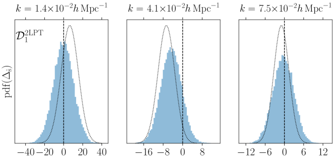
As a final remark, we also show the posterior of initial conditions within different -bins in Fig. 13. As anticipated already in Fig. 4, the posterior is indeed non-Gaussian, showing stronger deviations from the Gaussian case as one goes toward smaller scales (reflected in the heavier tails of the distribution). Furthermore, even on the largest scales covered by our simulated volume, the prediction from the Wiener filter is biased with respect to the inferred posterior which is correctly centered around the ground truth (see the left-most panel).
5.2.2 Biased tracers
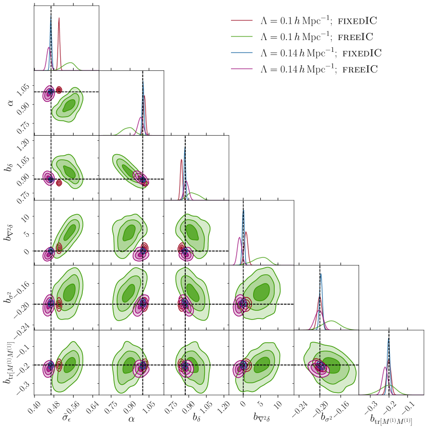
The synthetic datasets from Sec. 5.2.1 consisted merely of the evolved 2LPT matter field, rescaled by the linear bias with added Gaussian noise. Here, we consider synthetic datasets with nonzero higher-order bias coefficients, as well as a cutoff mismatch. This means that we test for the ability of our forward model to extract correct values from the biased tracers while marginalizing over plausible initial conditions realizations. As before, the dataset is generated using a cutoff , i.e. restricting to mildly nonlinear scales (recall that all synthetic data sets are at ). A more realistic test case would adopt dark matter halo or simulated galaxy fields identified in cosmological N-body or hydrodynamic simulations as input. We leave this for future work.
We show in Fig. 16 a comparison of the real-space posterior mean of our inference and the underlying ground-truth signal of the . As in Fig. 10, we also smooth with the same Gaussian kernel for aesthetic reasons. The overall trend of underdensities and overdensities is well captured by the posterior mean in this case as well. For a more quantitative analysis we present parameter posteriors next.
Since we currently do not have analytical predictions for the cutoff dependence of the bias coefficients, we focus instead on the value of as a measure of the model performance. Being a cosmological parameter, it should be consistent across different cutoffs .
We present here the results using the unmarginalized likelihood from Eq. (2.15), shown in Fig. 17. We find a difference between the fiducial noise level and the one inferred at a lower cutoff, similar to the case in Sec. 5.1.2. The reason is the same as there, namely the presence of second-order bias terms in the dataset and the fact that . Estimating this shift could be done similarly as in Eq. (5.4), but taking into account the presence of higher-order nonlinear terms. We leave this calculation for future work.
Turning to the parameter, both the (blue) and (red) fixedIC posteriors consistently infer the correct value as expected. For the freeIC case, the forward model posterior (purple contours) is able to recover the fiducial value and is furthermore consistent with the corresponding fixedIC posterior (blue contours). However, the freeIC posterior (green contours) shows a preference for smaller , and excludes the fiducial value at contour. Similar systematic shifts can also be observed in the bias parameters.
6 Conclusions and Summary
In this paper, we have investigated the robustness of field-level inference based on the EFT framework with respect to a mismatch between theory and data, as well as the ability to constrain the amplitude of initial conditions () when marginalizing over the initial conditions. Such tests do not only probe the robustness of the chosen forward model and likelihood but also allow for a better understanding regarding what types of forward model physics are necessary in order to capture all relevant effects and to obtain unbiased inference of the cosmological parameters.
We have focused on several different types of forward models described in Sec. 2, each probing different limits of our modeling framework from Eq. (2.13), as well as different types of likelihood, one with explicit marginalization over bias parameters (Eq. (2.16)) and the other without (Eq. (2.15)). We perform all the tests on a suite of synthetic datasets with realistic noise levels, described in Sec. 4.
We have demonstrated in Sec. 5.1.1 that, in the case of the purely linear forward model (see Eq. (2.3)), our sampling approach coupled with the EFT likelihood attains a full exploration of the high-dimensional posterior, which in this case can be derived analytically (see Fig. 2–3 as well as the top panel of Fig. 4). This is a nontrivial result given the high-dimensional () posterior surface involved.
In Sec. 5.1.2 we have considered a simple but nontrivial extension by adding the term in the bias expansion as given in Eq. (2.5). This term leads to a mode coupling between two linear density fields, which in turn yields a non-Gaussian posterior of the initial conditions, as can be seen from the bottom panel of Fig. 4 as well as Fig. 7. Nevertheless, the inferred parameters show the expected behavior also in this non-Gaussian case (Fig. 5). We further find good agreements between the fixedIC, where the initial conditions are fixed to their ground-truth values, and freeIC posteriors. This illustrates that our forward modeling and sampling approaches explore the posterior around the correct solution.
We have also examined cases that include a model mismatch in the 2LPT gravity model, by way of choosing a lower cutoff in the inference than the one used to generate the synthetic data. As synthetic datasets, we consider matter fields in Sec. 5.2.1 and nonlinearly biased tracer fields in Sec. 5.2.2, both including white Gaussian noise. For these cases, we find that, even in the presence of model mismatch, the EFT likelihood is still able to obtain unbiased estimates of cosmological parameters, specifically which is our proxy for . We have also demonstrated the advantage of using the marginalized over the unmarginalized likelihood from Eqs. (2.16)–(2.15) respectively, by showing a significantly reduced correlation length, in particular for .
We do find signs of a mild discrepancy in the inferred value in the case for the synthetic data set including nonlinear bias when also allowing for a mismatch. We leave the exploration of possible causes to upcoming work; while prior volume effects could be responsible, higher-order bias terms and density-dependent noise could also be relevant for this particular data set. The flexibility in generating different synthetic data sets will allow for a disentangling of the possible causes. Such future tests should also include the generalization to synthetic data involving nontrivial noise, such as scale- and density-dependent or non-Gaussian (for example, Poisson) noise.
Even though we focused on real-space realizations of the synthetic data and our forward model, we note that recent developments within the LEFTfield framework allow for a consistent treatment of the redshift-space distortions at any order within the EFT framework [38], although this has only been tested the fixedIC scenario for now. We leave the development of the corresponding freeIC sampling scheme, including the redshift-space distortions for future work.
Finally, while we are refraining from making a precise quantitative statement here, it is worth noting that the posteriors on obtained on our biased 2LPT mock data sets (Fig. 11 and Fig. 17; with average 68% CL errors on of and for and , respectively) are significantly tighter than what a Fisher forecast for joint power spectrum and bispectrum analysis yields on a similar configuration (cf. Sec. 4.1.3 of [35], for example). This will likewise be explored in more detail in upcoming work.
7 Acknowledgements
We thank Andrej Obuljen, Marko Simonović, Uroš Seljak, Matias Zaldariagga, Henrique Rubira for useful discussions during the Šmartno 2022 conference. AK thanks Philipp Frank for the discussion on the results of App. B.2 and Florent Leclercq for the discussion on higher-order symplectic integrator schemes for HMC. MN thanks Nickolas Kokron, Emmanuel Schaan, and Chirag Modi for useful discussions on model mis-specification, Wiener-filter solution, and HMC performance, respectively. The authors also thank Deaglan Bartlett, Eiichiro Komatsu, Henrique Rubira, and Julia Stadler for useful feedback on the initial manuscript, which significantly improved the quality of the text. The authors also thank the anonymous editor and referee for providing useful comments on the initial draft of the manuscript. AK and FS acknowledge support from the Starting Grant (ERC-2015-STG 678652) “GrInflaGal” of the European Research Council. MN acknowledges support from the Leinweber Foundation and the NASA grant under contract 19-ATP19-0058. All MCMC chains in this paper were produced on the HPC cluster FREYA, maintained by the Max Planck Computing & Data Facility. All 1D and 2D posterior plots shown in this paper were obtained through the use of a modified version of corner.py444https://corner.readthedocs.io/ [56]. This work has been done within the Aquila Consortium555https://www.aquila-consortium.org.
Appendix A Fourier space convention
Below, we summarize the Fourier convention and notation adopted throughout the paper. We give the explicit relation between the Fourier- and Hartley-representation of . The latter is of relevance for understanding our prior choices in Sec. 3.1 and following the calculations done in App. B.1 and App. B.2.
First, we define the forward Fourier transform and its inverse transform as
In practice, we operate on finite grids, thus we use the discrete Fourier transforms given by
where with , and . The Nyquist frequency is given by . stands for the box size. With this, the two-point function of the becomes
| (A.1) |
where , with representing the Kronecker delta. For clarity, we also write this Kronecker delta in wavenumber space as . For a field drawn from a unit normal distribution in real space, it follows that , and hence .
In order to implement the cutoff , we use the isotropic sharp- filter defined as
| (A.2) |
with being the Heaviside function.
Finally, we note that any field can be represented either in the Fourier or Hartley convention, with our LEFTfield code utilizing the latter. The two representations are related through (see [57] and Sec. 3.4 in [58] for more details)
| (A.3) |
with and denoting Fourier and Hartley transforms respectively. This is the field whose mean, residual, and variance are shown in the figures in Sec. 5.
Appendix B Gaussian expectation for posterior
In this section, we present efforts towards analytical understanding of the shapes of posteriors for the forward models represented by Eq. (2.3) (App. B.1) and Eq. (2.5) (App. B.2), restricting to the case where the bias parameters and noise amplitude are fixed to the ground truth. It is much more difficult to obtain an analytical expression for the posterior when also varying the latter.
In the linear case, an analytical form of the posterior exists, whose mean and variance coincide with the Wiener-filter solution (see, for example, [59, 60] and references therein). In the nonlinear case, however, only a perturbative approach is possible and we elaborate on this in App. B.2.
B.1 Linear model
As discussed around Eq. (2.3), the covariance structure of cosmological initial conditions is diagonal in Fourier space. Specifically, using the Fourier-space representation of our prior covariance (see our Fourier convention from App. A), one obtains
where represents the Kronecker delta. The noise is likewise assumed to be Gaussian with diagonal covariance related to (see Eq. (2.14)) as
These two assumptions allow us to derive the expected posterior on . In order to more easily see this, we can rephrase Eq. (2.3) as follows
where repeated indices are summed over; in the following, we will drop the repeated indices. We also drop the explicit dependence, since here we are only interested in the posterior of initial conditions with fixed to the ground truth. In the following, we will further fix the parameters and ; only for this case can we derive the posterior for analytically.
The likelihood for can be derived by marginalizing over the noise distribution, which yields
with denoting the mean and denoting the covariance of this Gaussian. Going forward, we consider log probabilities for convenience. This leads to (suppressing the conditional on parameters for clarity)
| (B.1) |
where and represent the total number of modes in the and fields, respectively. In our applications, these are always the same.
Defining and we can rewrite Eq. (B.1) as
| (B.2) |
where we have accumulated all the -independent terms inside , i.e.
| (B.3) |
It is now clear that the posterior of is Gaussian:
| (B.4) |
with mean and covariance given as
| (B.5) |
Substituting into the second line of Eq. (B.5) the expression for response , noise covariance and the prior yields the following expression for the posterior covariance
| (B.6) |
For the results shown in the main text, we calculate Eq. (B.6) for every mode. We note that when comparing our analytical expression from Eq. (B.6) to the results for the power spectrum obtained from sampling shown in the bottom panel of Fig. 3 and in Fig. 7, we account for the fact that is in fact distributed within each -bin. The shape parameter is given by , with being the number of modes within the Fourier space shell centered on , while the scale parameter is (see Sec. 5.1.1). We again emphasize that the posterior mean and variance Eq. (B.5) coincide with the Wiener filter result only for a linear forward model, Gaussian prior and likelihood, and fixed parameters . In fact, Fig. 7 indicates that the Wiener filter estimate of the residual variance is biased low, i.e. is relatively lower than the actual variance , for nonlinear forward models.
B.2 Quadratic model
We now consider the quadratic bias model with linearized gravity (see Eq. (2.5)). Readers are referred to App. A for our discrete Fourier convention. We start with writing out the full likelihood expression
dropping the explicit dependence since this parameter is held fixed for our forward model from Eq. (2.5). Writing explicitly the from Eq. (2.5) reads
| (B.7) |
with and operations defined as
| (B.8) |
Note that the operator is the same as that in the linear forward model described in App. B.1. The operator implements the second-order bias via a convolution in Fourier space, with the kernel represented by the product of the two transfer functions and the sharp- cutoffs.
We now add the Gaussian log-prior on to Eq. (B.7) and expand in powers of . This results in the following ordering of terms (repeated indices are summed over)
| (B.9) | ||||
In other words, the final log-posterior is given by (in matrix notation)
| (B.10) |
where we have introduced the third and fourth order coupling kernels with and respectively. Also, we have relabeled the operators in the quadratic and linear term with and respectively. In the absence of the term, the posterior covariance is given exactly by the Wiener-filter solution for posterior covariance, i.e. second line of Eq. (B.5). For the posterior given in Eq. (B.10), it is not straightforward to compute the corresponding first and second moments. Instead, we expand the posterior around the Wiener-filter solution. While this expansion is strictly only valid if the correction due to is small, this expansion nevertheless offers some interesting insights.
We thus define , where represents the Wiener filter prediction of the initial conditions given by Eq. (B.5). In this case, the formalism of Information Field Theory, as presented in [60], suggests the following diagrammatic representation of the solution (see also Sec. V.C of [60] and, for the Feynman rules, Sec. IV.A.2 of the same paper)
where the diagrams correspond to the following expressions
| (B.11) |
where we assume that the external lines (without dots) are fixed at and as indicated in the first line.
We can see that at leading order the posterior covariance is given exactly by , while the corrections to it depend on the exact form of the coupling kernels and . The evaluation of requires an explicit matrix inversion.
To avoid this, and keeping in mind that this expansion is only valid for small corrections to the Wiener-filter posterior, we expand to obtain the leading correction to the posterior covariance
| (B.12) |
Writing out the leading correction term, one obtains
| (B.13) |
This implies that the leading correction to the covariance around the Wiener-filter solution only contributes to the off-diagonal elements. This is an expected result, given the structure of the mode coupling introduced by the term from Eq. (2.5). In order to compute the correction to the diagonal part of the posterior covariance shown in Fig. 7, one would need to compute the next-to-leading correction to the posterior covariance. At this order, one also has to include the shift of the maximum of the posterior from the Wiener-filter solution, which is also of order . This is a more involved calculation which we leave for future work.
The considerations above indicate that obtaining even approximate analytical posteriors for is very difficult already for the simplest nonlinear models. These difficulties are correspondingly exacerbated for more nonlinear models, such as those involving LPT forward models. Thus, the explicit sampling approach appears to be the only path toward obtaining trustable posteriors for initial conditions inference using nonlinear forward models.
Appendix C Running of with the cutoff
In this section, we describe the 1-loop calculation of the expectation value of the parameter as a function of the forward model cutoff . In order to derive this relation, it is sufficient to look at the maximum likelihood point of the unmarginalized likelihood (see Eq. (2.15))
| (C.1) |
We have again suppressed the explicit dependence within , since for the forward model from Eq. (2.5) we keep it fixed. Since is a constant, we can factor it out and using the fact that the forward model here is given by Eq. (2.5) one can rearrange the above Eq. (C.1) to obtain
where we have explicitly stated the cutoff dependence of the bias coefficients, which holds in general and used the fact that the density fluctuation field is hermitian.
Before proceeding, we note that the above equation holds for a given realization of initial conditions, as explicitly stated in Eq. (C.1).
In what follows, we evaluate the MAP relation for at the ground-truth initial conditions . This is obviously the correct choice when comparing to fixedIC chains. However, since is expected to be in the typical set of the freeIC posterior, the result can also be translated to freeIC chains. After evaluating on the ground truth, we then take the ensemble average over data realizations. This allows us to compute the result analytically and gives the following (see also section 3 of [2])
| (C.2) |
keeping only the non-zero correlators. Given that the procedure for evaluating all correlators is essentially the same, we focus only on the correlator from the left-hand side of Eq. (C.2). Hence, we get
Using repeated Wick contractions one gets
| (C.3) |
with representing the linear power spectrum. From the above equation, it is clear that the correlator is a diagonal matrix in Fourier space. Furthermore, using the fact that the sharp- cutoff cares only about the magnitude of the given -mode, we can rewrite Eq. (C.3) as
| (C.4) |
indicating that the second line only contributes to the mode, which is not included in the likelihood evaluation, so this line can be dropped from further consideration. Therefore, the only relevant piece is the loop integral on the first line, which in fact matches the correlator on the right-hand side of Eq. (C.2). This shows that , and hence no running of is expected for the forward model represented by Eq. (2.5). This behavior is confirmed within our inference chains in Fig. 6. Note that this result is specific to this simple forward model, and does not apply to the LPT forward models.
| Forward model, | Dataset | |||
|---|---|---|---|---|
| linear - Eq. (2.3), | 113 | |||
| linear - Eq. (2.3), | 320 | |||
| linear - Eq. (2.3), | 230 | |||
| linear - Eq. (2.3), | 102 | |||
| linear - Eq. (2.5), | 1138 | |||
| linear - Eq. (2.5), | 933 | |||
| linear - Eq. (2.5), | 1051 | |||
| linear - Eq. (2.5), | 1075 | |||
| linear - Eq. (2.5), | 635 | |||
| linear - Eq. (2.5), | 622 | |||
| linear - Eq. (2.5), | 330 | |||
| linear - Eq. (2.5), | 277 | |||
| linear - Eq. (2.5), | 232 | |||
| linear - Eq. (2.5), | 288 | |||
| linear - Eq. (2.5), | 147 | |||
| linear - Eq. (2.5), | 195 | |||
| 1LPT - Eq. (2.11), | 256 | |||
| 1LPT - Eq. (2.11), | 135 | |||
| 1LPT - Eq. (2.11), | 171 | |||
| 1LPT - Eq. (2.11), | 114 | |||
| 2LPT - Eq. (2.11), | 273 | |||
| 2LPT - Eq. (2.11), | 243 | |||
| 2LPT - Eq. (2.11), | 311 | |||
| 2LPT - Eq. (2.11), | 385 | |||
| 2LPT - Eq. (2.11), | 184 | |||
| 2LPT - Eq. (2.11), | 157 | |||
| 2LPT - Eq. (2.11), | 125 | |||
| 2LPT - Eq. (2.11), | 103 |
| Forward model, | Dataset | |||
|---|---|---|---|---|
| linear - Eq. (2.5), | 1516 | |||
| linear - Eq. (2.5), | 1408 | |||
| linear - Eq. (2.5), | 469 | |||
| linear - Eq. (2.5), | 523 | |||
| linear - Eq. (2.5), | 224 | |||
| linear - Eq. (2.5), | 296 | |||
| linear - Eq. (2.5), | 132 | |||
| linear - Eq. (2.5), | 121 | |||
| linear - Eq. (2.5), | 205 | |||
| linear - Eq. (2.5), | 211 |
| Forward model, | Dataset | |||
|---|---|---|---|---|
| 1LPT - Eq. (2.11), | 128 | |||
| 1LPT - Eq. (2.11), | 108 | |||
| 1LPT - Eq. (2.11), | 155 | |||
| 1LPT - Eq. (2.11), | 145 | |||
| 2LPT - Eq. (2.11), | 166 | |||
| 2LPT - Eq. (2.11), | 156 | |||
| 2LPT - Eq. (2.11), | 185 | |||
| 2LPT - Eq. (2.11), | 174 | |||
| 2LPT - Eq. (2.11), | 137 | |||
| 2LPT - Eq. (2.11), | 129 | |||
| 2LPT - Eq. (2.11), | 131 | |||
| 2LPT - Eq. (2.11), | 192 |
Appendix D Chain convergence and sample correlation analysis
MCMC samples are not entirely independent. In practice, this correlation between neighboring samples introduces further uncertainty in any estimate based on averaging over those samples, such as the posterior mean, variance, and all higher moments. The correlation is often measured by the integrated autocorrelation time, while the resulting uncertainty in the posterior is quantified by the effective sample size. We refer readers to [54] for more details.
We define the normalized autocorrelation function, , as
| (D.1) |
where is the set of chain samples, and the brackets indicate the average over samples, i.e. , while indicates the sample separation. Eq. (D.1) highlights the significance of having a sufficient number of MCMC samples, i.e. running sufficiently long MCMC chains, since and are noisy estimates of the true mean and variance, whose noise propagates nonlinearly into . For the autocorrelation function, , we use the estimator presented in [61] which shows better asymptotic behavior than the one given in Eq. (D.1). The normalized autocorrelation function is exactly what is shown in Fig. 12. We then use the to estimate the correlation length of the chain as
| (D.2) |
with representing the maximal separation between the samples considered. This estimator has a vanishing variance in the limit of large chain lengths, i.e. number of samples. We have adopted the approach of [62] for choosing . In short, is chosen such that it corresponds to the smallest integer satisfying with a constant chosen such that the variance of the estimator is minimized, at the cost of introducing a negative bias in the estimate of . This is typically achieved for . We report the estimates, as well as the used window in Fig. 12, when comparing the sampling performance of the marginalized and unmarginalized likelihood.
We now describe the two tests of convergence we perform for all chains analyzed in this paper, namely the classical and revised Gelman-Rubin (G-R) diagnostic. The revised G-R statistics [55] makes a clear connection to the chain effective sample size (see Eq. (12) in [55]). We exploit this connection to link the (revised) G-R value and our target effective sample size.
For the classical G-R statistics [53, 63, 54], we adopt the following procedure. First we calculate the inter- and intra-chain variances
| (D.3) |
with
and , being the chain length and number of chains considered respectively. From the above expression, one can see that represents an estimate of the variance between the chains while is the mean of the variance within individual chains. These two quantities then can be combined into an estimate of the true underlying target distribution variance
| (D.4) |
The authors of [53, 63] argue that for a properly dispersed set of chains, the estimate is typically over-estimating the underlying variance, while the mean of the within-the-chain variances, , under-estimates it. Hence, they propose the following quantity as a measure of chain convergence, which is known as the classical G-R test statistics
| (D.5) |
Specifically, we apply this univariate G-R test to the parameter (for chains from Sec. 4.2) and parameter (for chains from Sec. 5.1), since these parameters typically have the longest correlation lengths and largest values. The resulting values are reported in Tab. 2, 3 and 4 as .
The revised G-R test statistics can be estimated from the following expression
| (D.6) |
The above Eq. (D.6) provides a clear connection between the number of chains , effective sample size and the convergence threshold . It is possible to determine the convergence threshold a priori and hence the corresponding effective size necessary for reaching it. Specifically, in this paper, we set a target of for all MCMC chains. In practice, we use the n.eff multivariate method of the stable.GR package666https://github.com/knudson1/stableGR to estimate . The stable.GR package is provided by the authors of [55]. For more details on how is calculated, we refer readers to Sec. 5 of [55]. This number is reported in the last column of Tab. 2, 3 and 4. We note that the convergence threshold value we report represents an ideal case, which corresponds to having the same number of chains as we do, but with of samples lying within of the posterior volume around the posterior mean. Such chains will then have .
Appendix E Relation between 1LPT and 2LPT second-order bias coefficients
As described in Sec. 2, the 1LPT and 2LPT forward models differ only in the order of the LPT displacement field. This difference has an impact on the inference as shown in Fig. 11. The goal of this section is to understand whether the observed discrepancy between the 1LPT and 2LPT posteriors is expected. In order to derive this, we first go back to the general setup of both of these models.
First, the same order of Lagrangian bias expansion is employed in both, allowing for the following set of Lagrangian bias operators
| (E.1) |
and the corresponding bias coefficients. Recall that we displace a unit field to obtain the Eulerian matter density. The transformation of bias coefficients derived in the following only involves operators at leading order in derivatives, therefore we do not need to consider in the following. The relation between Eulerian and Lagrangian frames is given by [35]
| (E.2) |
with being the Jacobian of the transformation from Lagrangian to Eulerian coordinates, and denoting the order up to which the forward model is to be evaluated. Note that in our field-level forward model, is computed non-perturbatively, by displacing and depositing pseudo particles within the simulated box. Here, we instead expand perturbatively up to second order, to obtain the mapping of bias operators between the different LPT orders. Specifically, for 1LPT and 2LPT the corresponding inverse Jacobians are given by
| (E.3) |
where we kept only second-order terms. We then use the following bias expansion
| (E.4) |
where we note that is the coefficient of the uniform field . Plugging the results of Eqs. (E.3)–(E.4) directly into the first line of Eq. (E.2) we obtain
| (E.5) |
again keeping only second-order terms. In Eq. (E.5) we also used the solution for the second order displacement field from the equations of motion assuming an Einstein-de Sitter universe (see [42], as well as Sec. 2.7 in [64], Sec. 2.5.2 in [35])
This then produces the following relationship between the 1LPT and 2LPT forward model bias coefficients
| (E.6) |
We can now compare with the results from the 1LPT and 2LPT posteriors obtained on the datasets, shown in Fig. 11. Taking the mean of the 2LPT posterior for and , leads to and , which are indicated with dotted lines in Fig. 11, which agree within confidence level with the obtained 1LPT posterior.
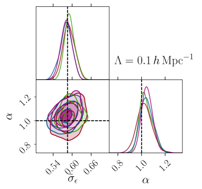
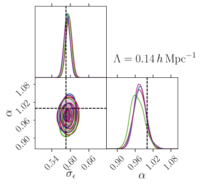
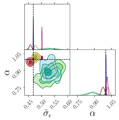
Appendix F Marginalized and unmarginalized likelihood chains
Here, we provide the posteriors obtained with the marginalized likelihood (Eq. (2.16)), using the priors given in Eq. (3.3).
Fig. 18 shows the posteriors of the forward model from Eq. (2.11) obtained on the dataset. We find the same results for the inference done on dataset. We contrast the marginalized likelihood posteriors (red and blue) to the unmarginalized (Eq. (2.15)) likelihood posteriors (green and purple), using the priors from Sec. 3.1. The posterior contours are entirely consistent with each other for both 1LPT and 2LPT forward models, and across the different cutoffs ( and ). However, recall that the marginalized likelihood leads to better efficiency in terms of sampling the parameter, as depicted in Fig. 12 (top panel).
The posterior of the same forward model obtained on the dataset, using the marginalized likelihood, is shown in Fig. 19. The results for the forward model with cutoff , turquoise and light-green for the freeIC case and the purple for the fixedIC posterior, all show higher levels of noise than the corresponding cases for posteriors. As discussed in Sec. 5.2.2, this is a consequence of the mode couplings present at the higher cutoff at which the synthetic datasets were generated (see also Sec. 5.1.2). It is as well worth noting that the posteriors obtained with the marginalized likelihood from Fig. 19 are consistent with the corresponding unmarginalized case shown in Fig. 17.
References
- [1] F. Schmidt, An n-th order Lagrangian forward model for large-scale structure, JCAP 2021 (2021) 033 [2012.09837].
- [2] F. Schmidt, F. Elsner, J. Jasche, N.M. Nguyen and G. Lavaux, A rigorous EFT-based forward model for large-scale structure, JCAP 2019 (2019) 042 [1808.02002].
- [3] F. Elsner, F. Schmidt, J. Jasche, G. Lavaux and N.-M. Nguyen, Cosmology inference from a biased density field using the EFT-based likelihood, JCAP 2020 (2020) 029 [1906.07143].
- [4] F. Schmidt, G. Cabass, J. Jasche and G. Lavaux, Unbiased cosmology inference from biased tracers using the EFT likelihood, JCAP 2020 (2020) 008 [2004.06707].
- [5] G. Cabass and F. Schmidt, The EFT likelihood for large-scale structure, JCAP 2020 (2020) 042 [1909.04022].
- [6] G. Cabass and F. Schmidt, The likelihood for LSS: stochasticity of bias coefficients at all orders, JCAP 2020 (2020) 051 [2004.00617].
- [7] F. Schmidt, Sigma-eight at the percent level: the EFT likelihood in real space, JCAP 2021 (2021) 032 [2009.14176].
- [8] DESI Collaboration, The DESI Experiment Part I: Science,Targeting, and Survey Design, arXiv e-prints (2016) arXiv:1611.00036 [1611.00036].
- [9] L. Amendola, S. Appleby, A. Avgoustidis, D. Bacon, T. Baker, M. Baldi et al., Cosmology and fundamental physics with the Euclid satellite, Living Reviews in Relativity 21 (2018) 2 [1606.00180].
- [10] M. Takada, R.S. Ellis, M. Chiba, J.E. Greene, H. Aihara, N. Arimoto et al., Extragalactic science, cosmology, and galactic archaeology with the subaru prime focus spectrograph, Publications of the Astronomical Society of Japan 66 (2014) .
- [11] P.A. Abell, J. Allison, S.F. Anderson, J.R. Andrew, J.R.P. Angel, L. Armus et al., Lsst science book, version 2.0, arXiv preprint arXiv:0912.0201 (2009) .
- [12] S. Alam, M. Aubert, S. Avila, C. Balland, J.E. Bautista, M.A. Bershady et al., Completed SDSS-IV extended Baryon Oscillation Spectroscopic Survey: Cosmological implications from two decades of spectroscopic surveys at the Apache Point Observatory, Phys. Rev. D 103 (2021) 083533 [2007.08991].
- [13] H. Gil-Marín, J. Noreña, L. Verde, W.J. Percival, C. Wagner, M. Manera et al., The power spectrum and bispectrum of SDSS DR11 BOSS galaxies - I. Bias and gravity, MNRAS 451 (2015) 539 [1407.5668].
- [14] H. Gil-Marín, W.J. Percival, L. Verde, J.R. Brownstein, C.-H. Chuang, F.-S. Kitaura et al., The clustering of galaxies in the SDSS-III Baryon Oscillation Spectroscopic Survey: RSD measurement from the power spectrum and bispectrum of the DR12 BOSS galaxies, MNRAS 465 (2017) 1757 [1606.00439].
- [15] O.H.E. Philcox and M.M. Ivanov, BOSS DR12 full-shape cosmology: CDM constraints from the large-scale galaxy power spectrum and bispectrum monopole, Phys. Rev. D 105 (2022) 043517 [2112.04515].
- [16] G. D’Amico, Y. Donath, M. Lewandowski, L. Senatore and P. Zhang, The BOSS bispectrum analysis at one loop from the Effective Field Theory of Large-Scale Structure, arXiv e-prints (2022) arXiv:2206.08327 [2206.08327].
- [17] D. Gualdi and L. Verde, Integrated trispectrum detection from BOSS DR12 NGC CMASS, JCAP 2022 (2022) 050 [2201.06932].
- [18] O.H.E. Philcox, Probing parity violation with the four-point correlation function of BOSS galaxies, Phys. Rev. D 106 (2022) 063501 [2206.04227].
- [19] J. Hou, Z. Slepian and R.N. Cahn, Measurement of Parity-Odd Modes in the Large-Scale 4-Point Correlation Function of SDSS BOSS DR12 CMASS and LOWZ Galaxies, arXiv e-prints (2022) arXiv:2206.03625 [2206.03625].
- [20] J. Jasche and B.D. Wandelt, Bayesian physical reconstruction of initial conditions from large-scale structure surveys, MNRAS 432 (2013) 894 [1203.3639].
- [21] H. Wang, H.J. Mo, X. Yang, Y.P. Jing and W.P. Lin, ELUCID—Exploring the Local Universe with the Reconstructed Initial Density Field. I. Hamiltonian Markov Chain Monte Carlo Method with Particle Mesh Dynamics, ApJ 794 (2014) 94 [1407.3451].
- [22] J. Jasche and G. Lavaux, Physical Bayesian modelling of the non-linear matter distribution: New insights into the nearby universe, A&A 625 (2019) A64 [1806.11117].
- [23] G. Lavaux, J. Jasche and F. Leclercq, Systematic-free inference of the cosmic matter density field from SDSS3-BOSS data, arXiv e-prints (2019) arXiv:1909.06396 [1909.06396].
- [24] F.-S. Kitaura, M. Ata, S.A. Rodríguez-Torres, M. Hernández-Sánchez, A. Balaguera-Antolínez and G. Yepes, COSMIC BIRTH: efficient Bayesian inference of the evolving cosmic web from galaxy surveys, MNRAS 502 (2021) 3456 [1911.00284].
- [25] E.G.P. Bos, F.-S. Kitaura and R. van de Weygaert, Bayesian cosmic density field inference from redshift space dark matter maps, MNRAS 488 (2019) 2573 [1810.05189].
- [26] I. Babić, F. Schmidt and B. Tucci, BAO scale inference from biased tracers using the EFT likelihood, JCAP 2022 (2022) 007 [2203.06177].
- [27] N. Porqueres, D. Kodi Ramanah, J. Jasche and G. Lavaux, Explicit Bayesian treatment of unknown foreground contaminations in galaxy surveys, A&A 624 (2019) A115 [1812.05113].
- [28] N.-M. Nguyen, F. Schmidt, G. Lavaux and J. Jasche, Impacts of the physical data model on the forward inference of initial conditions from biased tracers, JCAP 2021 (2021) 058 [2011.06587].
- [29] D. Kodi Ramanah, T. Charnock and G. Lavaux, Painting halos from cosmic density fields of dark matter with physically motivated neural networks, Phys. Rev. D 100 (2019) 043515 [1903.10524].
- [30] T. Charnock, G. Lavaux, B.D. Wandelt, S. Sarma Boruah, J. Jasche and M.J. Hudson, Neural physical engines for inferring the halo mass distribution function, MNRAS 494 (2020) 50 [1909.06379].
- [31] C. Modi, Y. Feng and U. Seljak, Cosmological reconstruction from galaxy light: neural network based light-matter connection, JCAP 2018 (2018) 028 [1805.02247].
- [32] D. Baumann, A. Nicolis, L. Senatore and M. Zaldarriaga, Cosmological non-linearities as an effective fluid, JCAP 7 (2012) 51 [1004.2488].
- [33] S.M. Carroll, S. Leichenauer and J. Pollack, Consistent effective theory of long-wavelength cosmological perturbations, Phys. Rev. D 90 (2014) 023518 [1310.2920].
- [34] J.J.M. Carrasco, M.P. Hertzberg and L. Senatore, The effective field theory of cosmological large scale structures, Journal of High Energy Physics 2012 (2012) 82 [1206.2926].
- [35] V. Desjacques, D. Jeong and F. Schmidt, Large-scale galaxy bias, Phys. Rep. 733 (2018) 1 [1611.09787].
- [36] O.H.E. Philcox, M.M. Ivanov, G. Cabass, M. Simonović, M. Zaldarriaga and T. Nishimichi, Cosmology with the redshift-space galaxy bispectrum monopole at one-loop order, Phys. Rev. D 106 (2022) 043530 [2206.02800].
- [37] M. Schmittfull, M. Simonović, V. Assassi and M. Zaldarriaga, Modeling biased tracers at the field level, Phys. Rev. D 100 (2019) 043514 [1811.10640].
- [38] J. Stadler, F. Schmidt and M. Reinecke, Cosmology inference at the field level from biased tracers in redshift-space, arXiv e-prints (2023) arXiv:2303.09876 [2303.09876].
- [39] C. Rampf, The recursion relation in Lagrangian perturbation theory, JCAP 12 (2012) 4 [1205.5274].
- [40] V. Zheligovsky and U. Frisch, Time-analyticity of Lagrangian particle trajectories in ideal fluid flow, Journal of Fluid Mechanics 749 (2014) 404 [1312.6320].
- [41] T. Matsubara, Recursive solutions of Lagrangian perturbation theory, Phys. Rev. D 92 (2015) 023534 [1505.01481].
- [42] T. Buchert, Lagrangian theory of gravitational instability of Friedman-Lemaitre cosmologies and the ’Zel’dovich approximation’, MNRAS 254 (1992) 729.
- [43] M. Mirbabayi, F. Schmidt and M. Zaldarriaga, Biased tracers and time evolution, JCAP 7 (2015) 30 [1412.5169].
- [44] A. Barreira, T. Lazeyras and F. Schmidt, Galaxy bias from forward models: linear and second-order bias of IllustrisTNG galaxies, JCAP 2021 (2021) 029 [2105.02876].
- [45] T. Lazeyras, A. Barreira and F. Schmidt, Assembly bias in quadratic bias parameters of dark matter halos from forward modeling, JCAP 2021 (2021) 063 [2106.14713].
- [46] D.J.C. Mackay, Information Theory, Inference and Learning Algorithms (2003).
- [47] R.M. Neal, Slice Sampling, arXiv e-prints (2000) physics/0009028 [physics/0009028].
- [48] M. Betancourt, A Conceptual Introduction to Hamiltonian Monte Carlo, arXiv e-prints (2017) arXiv:1701.02434 [1701.02434].
- [49] R. Neal, MCMC Using Hamiltonian Dynamics, in Handbook of Markov Chain Monte Carlo, pp. 113–162 (2011), DOI.
- [50] J. Mannseth, T. Selland Kleppe and H.J. Skaug, On the application of higher order symplectic integrators in Hamiltonian Monte Carlo, arXiv e-prints (2016) arXiv:1608.07048 [1608.07048].
- [51] M. Hernández-Sánchez, F.-S. Kitaura, M. Ata and C. Dalla Vecchia, Higher order Hamiltonian Monte Carlo sampling for cosmological large-scale structure analysis, MNRAS 502 (2021) 3976 [1911.02667].
- [52] Y. Feng, U. Seljak and M. Zaldarriaga, Exploring the posterior surface of the large scale structure reconstruction, Journal of Cosmology and Astroparticle Physics 2018 (2018) 043.
- [53] A. Gelman and D.B. Rubin, Inference from Iterative Simulation Using Multiple Sequences, Statistical Science 7 (1992) 457.
- [54] A. Gelman, J.B. Carlin, H.S. Stern and D.B. Rubin, Bayesian data analysis, Chapman and Hall/CRC (1995).
- [55] D. Vats and C. Knudson, Revisiting the gelman–rubin diagnostic, Statistical Science 36 (2021) 518 [1812.09384].
- [56] D. Foreman-Mackey, corner.py: Scatterplot matrices in Python, The Journal of Open Source Software 1 (2016) 24.
- [57] K.J. Olejniczak, The hartley transform, The Transforms and Applications Handbook (2000) 281.
- [58] K. Jones, The regularized fast Hartley transform: optimal formulation of real-data fast Fourier transform for silicon-based implementation in resource-constrained environments, Springer Science & Business Media (2010).
- [59] F.S. Kitaura and T.A. Enßlin, Bayesian reconstruction of the cosmological large-scale structure: methodology, inverse algorithms and numerical optimization, MNRAS 389 (2008) 497 [0705.0429].
- [60] T.A. Enßlin, M. Frommert and F.S. Kitaura, Information field theory for cosmological perturbation reconstruction and nonlinear signal analysis, Phys. Rev. D 80 (2009) 105005 [0806.3474].
- [61] A. Sokal, Monte carlo methods in statistical mechanics: foundations and new algorithms, in Functional integration, pp. 131–192, Springer (1997).
- [62] N. Madras and A.D. Sokal, The pivot algorithm: a highly efficient monte carlo method for the self-avoiding walk, Journal of Statistical Physics 50 (1988) 109.
- [63] S.P. Brooks and A. Gelman, General methods for monitoring convergence of iterative simulations, Journal of computational and graphical statistics 7 (1998) 434.
- [64] F. Bernardeau, S. Colombi, E. Gaztanaga and R. Scoccimarro, Large-scale structure of the universe and cosmological perturbation theory, Physics reports 367 (2002) 1 [astro-ph/0112551].