Cosmic-ray Boron Flux Measured from 8.4 GeV$/n$ to 3.8 TeV$/n$
with the Calorimetric Electron Telescope
on the International Space Station

Abstract

We present the measurement of the energy dependence of the boron flux in cosmic rays and its ratio to the carbon flux in an energy interval from 8.4 GeV$/n$ to 3.8 TeV$/n$ based on the data collected by the CALorimetric Electron Telescope (CALET) during $\sim 6.4$ years of operation on the International Space Station. An update of the energy spectrum of carbon is also presented with an increase in statistics over our previous measurement. The observed boron flux shows a spectral hardening at the same transition energy $E_{0}\sim 200$ GeV$/n$ of the C spectrum, though B and C fluxes have different energy dependences. The spectral index of the B spectrum is found to be $\gamma=-3.047\pm 0.024$ in the interval $25<E<200$ GeV$/n$. The B spectrum hardens by $\Delta\gamma_{B}=0.25\pm 0.12$, while the best fit value for the spectral variation of C is $\Delta\gamma_{C}=0.19\pm 0.03$. The B/C flux ratio is compatible with a hardening of $0.09\pm 0.05$, though a single power-law energy dependence cannot be ruled out given the current statistical uncertainties. A break in the B/C ratio energy dependence would support the recent AMS-02 observations that secondary cosmic rays exhibit a stronger hardening than primary ones. We also perform a fit to the B/C ratio with a leaky-box model of the cosmic-ray propagation in the Galaxy in order to probe a possible residual value $\lambda_{0}$ of the mean escape path length $\lambda$ at high energy. We find that our B/C data are compatible with a non-zero value of $\lambda_{0}$, which can be interpreted as the column density of matter that cosmic rays cross within the acceleration region.

I Introduction

The larger relative abundance of light elements such as Li, Be, B in cosmic rays (CR) compared to the solar system abundance is a proof of their secondary origin. They are produced by the spallation reactions of primary CR, injected and accelerated in astrophysical sources, with nuclei of the interstellar medium (ISM). Measurements of the secondary-to-primary abundance ratios (as B/C) make it possible to probe galactic propagation models and constrain their parameters, since they are expected to be proportional at high energy to the average amount of material $\lambda$ traversed by CR in the Galaxy, which in turn is inversely proportional to the CR diffusion coefficient $D$. Earlier measurements Engelmann et al. (1990); Swordy et al. (1990); Ahn et al. (2008); Obermeier et al. (2012); Adriani et al. (2014) indicate that $\lambda$ decreases with increasing CR energy per nucleon $E$, following a power-law $\lambda\propto E^{-\delta}$, where $\delta$ is the diffusion spectral index. The recently observed hardening in the spectrum of CR of different nuclear species Aguilar et al. (2016, 2018, 2021b); Adriani et al. (2019, 2022); An et al. (2019); Alemanno et al. (2019) can be explained as due to subtle effects of CR transport including: an inhomogeneous or an energy-dependent diffusion coefficient Tomassetti (2012); Aloisio (2015); Johannesson et al. (2016); the possible re-acceleration of secondary particles when they occasionally cross a supernova shock during propagation Cuoco (2021); and/or the production of a small fraction of secondaries by interactions of primary nuclei with matter (source grammage) inside the acceleration region Cowsik (2021); Bresci (2019); Evoli (2019). To investigate these phenomena, a precise determination of the energy dependence of $\lambda$ is needed. That can be achieved by extending the measurements of secondary CR in the TeV$/n$ region with high statistics and reduced systematic uncertainties. In this Letter, we present new direct measurements of the energy spectra of boron, carbon and of the boron-to-carbon ratio in the energy range from 8.4 GeV$/n$ to 3.8 TeV$/n$, based on the data collected by the CALorimetric Electron Telescope (CALET) Torii and Marrocchesi (2019); Adriani et al. (2018, 2019) from October 13, 2015 to February 28, 2022 aboard the International Space Station (ISS).

II Detector

The CALET instrument comprises a CHarge Detector (CHD), a finely segmented pre-shower IMaging Calorimeter (IMC), and a Total AbSorption Calorimeter (TASC). A complete description of the instrument can be found in the Supplemental Material (SM) of Ref. Adriani et al. (2017).

The IMC consists of 7 tungsten plates interspaced with eight double layers of scintillating fibers, arranged along orthogonal directions. Fiber signals are used to reconstruct the CR particle trajectory by applying a combinatorial Kalman filter Maestro and Mori (2017). The estimated error in the determination of the arrival direction of B and C nuclei is $\sim 0.1^{\circ}$ with a corresponding spatial resolution of the impact point on the CHD of $\sim$220 $\mu$m.

The identification of the particle charge $Z$ is based on the measurements of the ionization deposits in the CHD and IMC. The CHD, located above the IMC, is comprised of two hodoscopes (CHDX, CHDY) made of 14 plastic scintillator paddles each, arranged perpendicularly to each other. The particle trajectory is used to identify the CHD paddles and IMC fibers traversed by the primary particle and to determine the path length correction to be applied to the signals to extract samples of the ionization energy loss ($dE/dx$). Three charge values ($Z_{\rm{CHDX}}$, $Z_{\rm{CHDY}}$, $Z_{\rm{IMC}}$) are reconstructed, on an event-by-event basis, from the measured $dE/dx$ in each CHD layer and the average of the $dE/dx$ samples along the track in the top half of IMC Adriani et al. (2019). The CHD can resolve individual chemical elements from $Z=1$ to 40, while the saturation of the fiber signals limits the IMC charge measurement to $Z\lesssim 14$. The charge resolution of the CHD (IMC) is $\sim 0.15\,(0.24)\,e$ (charge unit) in the elemental range from B to O.

The TASC is a homogeneous calorimeter made of 12 layers of lead-tungstate bars, each read out by photosensors and a front-end electronics spanning a dynamic range $>10^{6}$. The total thickness of the instrument is equivalent to 30 radiation lengths and 1.3 proton nuclear interaction lengths.

The TASC was calibrated at the CERN SPS in 2015 using a beam of accelerated ion fragments with $A/Z=2$ and kinetic energy of 13, 19 and 150 GeV$/n$ Akaike (2015). The response curve for interacting particles of each nuclear species is nearly gaussian at a fixed beam energy. The mean energy released in the TASC is $\sim$20% of the particle energy and the resolution is close to 30%. The energy response of the TASC turned out to be linear up to the maximum particle energy (6 TeV) available at the beam, as described in the SM of Ref. Adriani et al. (2019).

Monte Carlo (MC) simulations, reproducing the detailed detector configuration, physics processes, as well as detector signals, are based on the EPICS simulation package Kasahara (1995) and employ the hadronic interaction model DPMJET-III Roesler et al. (2000). Independent simulations based on Geant4 10.5 Allison et al. (2011) are used to assess the systematic uncertainties.

III Data analysis

We have analyzed flight data (FD) collected in 2331 days of CALET operation aboard the ISS. Raw data are corrected for non-uniformity in light output, time and temperature dependence, and gain differences among the channels by using penetrating protons and He particles selected by a dedicated trigger mode Asaoka et al. (2018). Correction curves for the reduction of the scintillator light yield due to the quenching effect in the CHD and IMC are obtained from FD by fitting subsets for each nuclear species to a function of $Z^{2}$ using a “halo” model Marrocchesi et al. (2011).

Boron and carbon candidates are searched for among events selected by the onboard high-energy (HE) shower trigger, which requires the coincidence of the summed signals of the last two IMC double layers and the top TASC layer. The total observation live time for the HE trigger is $T=4.72\times 10^{4}$ hours, corresponding to 87.2% of the total observation time. In order to mitigate the effect of possible temporal variations of the trigger thresholds on the trigger efficiency, an offline trigger is applied to FD with higher thresholds than the onboard trigger. Triggered particles entering the instrument from lateral sides or late-interacting in the lower half of the calorimeter are rejected based on the large fraction of energy leakage estimated from the shape of the longitudinal and lateral shower profiles. All reconstructed events with one well-fitted track passing through the top surface of the CHD and the bottom surface of the TASC (excluding a border region of 2 cm) are then selected. The geometrical acceptance for this category of events is $S\Omega\sim$510 cm²sr.

Boron and carbon candidates are identified by applying window charge cuts of half-width $0.45\,e$ centered on the nominal values ($Z=5,6$) to the distribution of the average charge in the CHD ($Z_{\rm{CHD}}$) obtained after requiring that $Z_{\rm{CHDX}}$ and $Z_{\rm{CHDY}}$ are consistent with each other within 10% and $|Z_{\rm{CHD}}-Z_{\rm{IMC}}|<1$, as shown in Fig. S2 of the SM PRL . The consistency of the charge values measured by each of the four upper IMC fiber layers is also required.

An additional cut on the track width ($\rm{TW}$) is applied to reject particles undergoing a charge-changing nuclear interaction in the upper part of the instrument. The $\rm{TW}$ variable is defined as the difference, normalized to the particle charge, between the total energy deposited in the clusters of nearby fibers crossed by the reconstructed track and the sum of the fiber signals in the cluster cores. Examples of $\rm{TW}$ distributions are shown in Fig. S3 of the SM PRL .

The field-of-view (FOV) of CALET at large zenith angle ($>$45^∘) is partially shielded by fixed structures on the ISS. Moreover, moving structures (e.g. solar panels, robotic arms) can cross the FOV for short periods of time during ISS operations. CR interactions in these structures can create secondary nuclei that, if detected by CALET, may induce a contamination in the flux measurements. To avoid that, the events ($\sim$8% of the final candidate samples) with reconstructed trajectories pointing to obstacles in the FOV are discarded in the analysis.

With this selection procedure 1.99$\times 10^{5}$ B and 9.27$\times 10^{5}$ C nuclei are identified. For flux measurements, an iterative unfolding Bayesian method D’Agostini (1995) is applied to correct the distributions (Fig. S4 of the SM PRL ) of the total energy deposited in the TASC ($E_{\rm TASC}$) for significant bin-to-bin migration effects (due to the limited energy resolution) and infer the primary particle energy. The response matrix for the unfolding procedure is derived using MC simulations after applying the same selection procedure as for FD. The energy spectrum is obtained from the unfolded energy distribution as follows:

$$\Phi(E)=\frac{N(E)}{\Delta E\;\varepsilon(E)\;S\Omega\;T}$$ (1)

$$N(E)=U\left[N_{obs}(E_{\rm TASC})-N_{bg}(E_{\rm TASC})\right]$$ (2)

where: $\Delta E$ is the energy bin width; $E$ the kinetic energy per nucleon calculated as the geometric mean of the lower and upper bounds of the bin; $N(E)$ the bin content in the unfolded distribution; $\varepsilon(E)$ the total selection efficiency (Fig. S5 of the SM PRL ); $U()$ the iterative unfolding procedure; $N_{obs}(E_{\rm TASC})$ the bin content of the observed energy distribution (including background); $N_{bg}(E_{\rm TASC})$ the bin content of background events in the observed energy distribution. The background contamination in the final B sample is estimated from $\rm{TW}$ distributions in different intervals of $E_{\rm TASC}$, after applying the complete charge selection procedure. The contamination fraction $N_{bg}/N_{obs}$ is $\sim 1\%$ for $E_{\rm TASC}<10^{2}$ GeV and grows logarithmically with $E_{\rm TASC}$ for $E_{\rm TASC}>10^{2}$ GeV, approaching $\sim 7\%$ at 1.5 TeV. The background is negligible for C.

IV Systematic Uncertainties

Different sources of systematic uncertainties were studied, including trigger efficiency, charge identification, energy scale, unfolding procedure, MC simulations, B isotopic composition, and background subtraction.

The HE trigger efficiency was measured as a function of $E_{\rm TASC}$ using a subset of data taken with a minimum bias trigger. The small differences ($<$1%) found between the HE efficiency curves and the predictions from MC simulations (Fig. S1 of the SM PRL ) induce a systematic error of $\pm 0.8\%$ ($\pm 0.7\%$) in the B (C) flux.

The systematic error related to charge identification was studied by varying the width of the window cuts for $Z_{\rm{CHD}}$ between 0.43 $e$ and 0.47 $e$ and the boundary $\alpha$ of the consistency cut $|Z_{\rm{CHD}}-Z_{\rm{IMC}}|<\alpha$ between 0.9 and 1.1. The result was a flux variation ranging from $-1.1\%$ to $3.1\%$ for B, and $-1.5\%$ to $0.9\%$ for C, depending on the energy bin.

The uncertainty ($\pm 2$%) in the energy scale from the beam test calibration affects the absolute normalization of the B and C spectra by $\pm$3% but not their shape.

The uncertainty due to the unfolding procedure was evaluated by using different response matrices computed by varying the spectral index of the generation spectrum of MC simulations. The resulting error in the absolute flux is $\pm 1.5\%$ for B and $\pm 0.5\%$ for C.

Since it is not possible to validate MC simulations with beam test data in the high-energy region, a comparison between different MC programs, i.e. EPICS and Geant4, was performed. We found that the selection efficiencies are similar, but the energy response matrices differ significantly in the low and high energy regions. The resulting fluxes for B (C) show discrepancies not exceeding 6% (10%) below 20 GeV$/n$ and 12% (10%) above 300 GeV$/n$, respectively. This is the dominant source of systematic uncertainties.

The uncertainty of the residual background contamination leads to a maximum error of $3\%$ in the B flux above 400 GeV$/n$, and $\leq 2\%$ below.

Since CALET cannot distinguish among the B isotopes, the spectral binning in kinetic energy per nucleon is calculated assuming an isotopic composition of 70% of ¹¹B and 30% of ¹⁰B as in Ref. Aguilar et al. (2016). We checked with MC that a variation of $\pm$10% in the abundance of ¹¹B causes a $\pm$1% difference in the selection efficiency and a $\mp$1.7% change in the flux normalization.

Other energy-independent systematic uncertainties affecting the normalization include live time (3.4%, as explained in the SM of Ref. Adriani et al. (2017)) and long-term stability of charge calibration ($0.5\%$).

The energy dependence of all the systematic uncertainties is shown in Fig. S6 of the SM PRL . Finally, an independent analysis, using different tracking and charge identification procedures Akaike and Maestro (2021), turned out to be in very good agreement with the results reported in this Letter.

V Results

The energy spectra of B and C and their flux ratio measured with CALET are shown in Fig. S8; the corresponding data tables including statistical and systematic errors are reported in the SM PRL . CALET spectra are compared with results from space-based Engelmann et al. (1990); Swordy et al. (1990); Adriani et al. (2014); Aguilar et al. (2021b, 2018) and balloon-borne Ahn et al. (2008); Obermeier et al. (2012); Panov et al. (2009); Ahn et al. (2009) experiments.

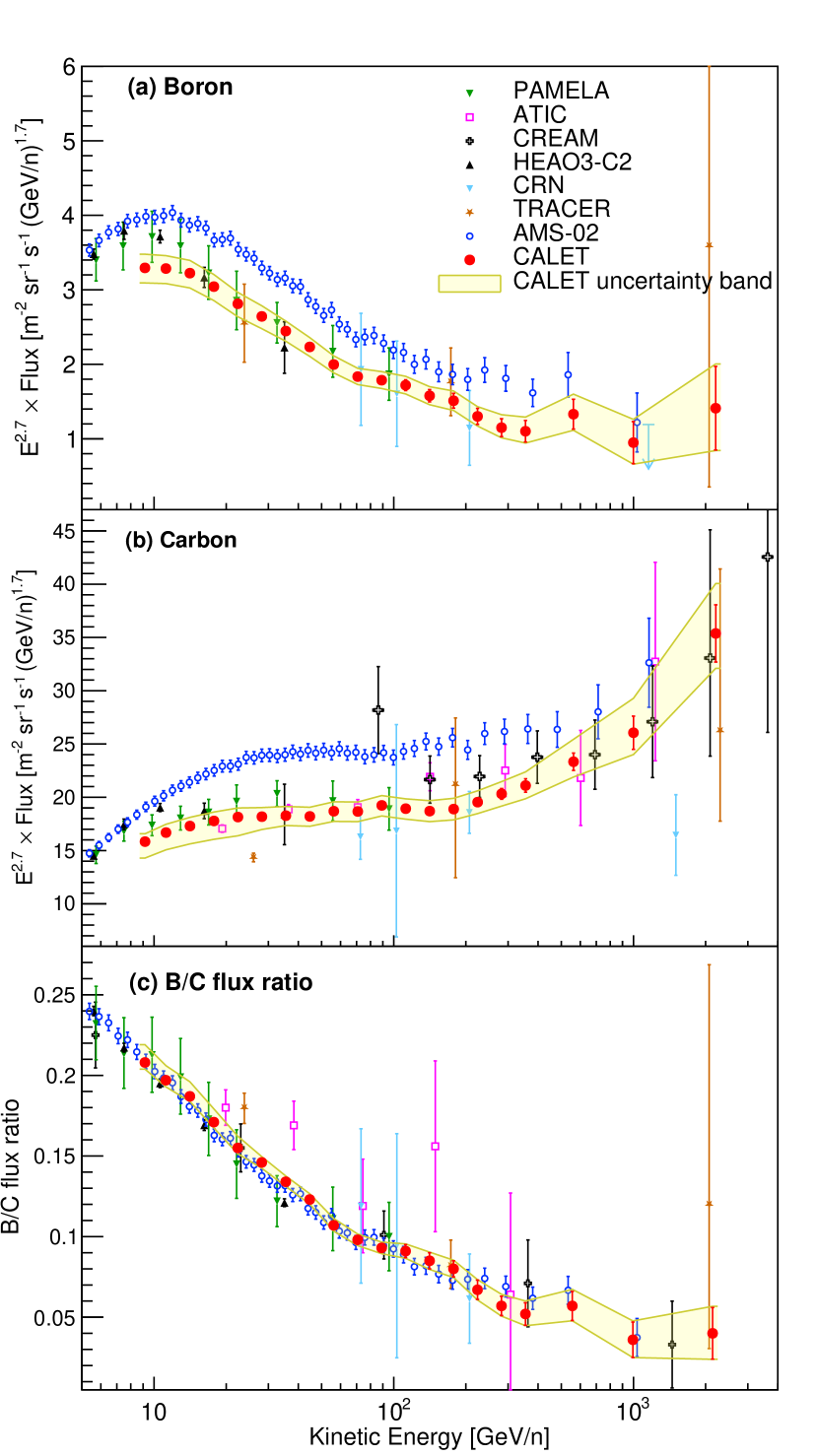
Figure 1: CALET (a) boron and (b) carbon flux (multiplied by $E^{2.7}$) and (c) ratio of boron to carbon, as a function of kinetic energy per nucleon $E$. Error bars of CALET data (red) represent the statistical uncertainty only, while the yellow band indicates the quadratic sum of statistical and systematic errors. Also plotted are other direct measurements Engelmann et al. (1990); Swordy et al. (1990); Ahn et al. (2008); Obermeier et al. (2012); Adriani et al. (2014); Aguilar et al. (2021b, 2018); Panov et al. (2009); Ahn et al. (2009). An enlarged version of the figure is available in Fig. S8 of the SM PRL .

The B spectrum is consistent with that of PAMELA Adriani et al. (2014) and most of the earlier experiments but the absolute normalization is in tension with that of AMS-02, as already pointed out by our previous measurements of the C, O and Fe fluxes Adriani et al. (2019, 2019). However we notice that the B/C ratio (Fig. S8(c)) is consistent with the one measured by AMS-02. The C spectrum shown here is based on a larger dataset but it is consistent with our earlier result and includes an improved assessment of systematic errors.

Figure 2 shows the fits to CALET B and C data with a double power-law function (DPL)

$$\Phi(E)=\begin{cases}c\left(\frac{E}{\text{GeV}}\right)^{\gamma}&E\leq E_{0}\\ c\left(\frac{E}{\text{GeV}}\right)^{\gamma}\left(\frac{E}{E_{0}}\right)^{\Delta\gamma}&E>E_{0}\end{cases}$$ (3)

where $c$ is a normalization factor, $\gamma$ the spectral index, and $\Delta\gamma$ the spectral index change above the transition energy $E_{0}$. A single power-law function (SPL) is also shown for comparison, where $\Delta\gamma=0$ is fixed in Eq. (3) and the fit is limited to data points with $25<E<200$ GeV$/n$ and extrapolated above. The DPL fit to the C spectrum in the energy range [25, 3800] GeV$/n$ yields $\gamma_{C}=-2.670\pm 0.005$ and a spectral index increase $\Delta\gamma_{C}=0.19\pm 0.03$ at $E_{0}^{C}=(220\pm 20)$ GeV$/n$ confirming our first results reported in Ref. Adriani et al. (2019). For the B spectrum, the parameter $E_{0}^{B}$ is fixed to the fitted value of $E_{0}^{C}$. The best fit parameters for B are: $\gamma_{B}=-3.047\pm 0.024$ and $\Delta\gamma_{B}=0.25\pm 0.12$ with $\chi^{2}/$d.o.f. = 11.9/12. The energy spectra are clearly different as expected for primary and secondary CR, and the fit results seem to indicate, albeit with low statistical significance, that the flux hardens more for B than for C above 200 GeV$/n$. A similar indication also comes from the fit to the B/C flux ratio (Fig. 3). In the energy range [25, 3800] GeV$/n$, it can be fitted with a SPL function with spectral index $\Gamma=-0.366\pm 0.018$ ($\chi^{2}/$d.o.f. = 9.4/13). However a DPL function provides a better fit suggesting a trend of the data towards a flattening of the B/C ratio at high energy, with a spectral index change $\Delta\Gamma=0.09\pm 0.05$ ($\chi^{2}/$d.o.f. = 8.7/12) above $E_{0}^{C}$, which is left as a fixed parameter in the fit. This result is consistent with that of AMS-02 Aguilar et al. (2018), and supports the hypothesis that secondary B exhibits a stronger hardening than primary C, although no definitive conclusion can be drawn due to the large uncertainty in $\Delta\Gamma$ given by our present statistics.

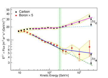
Figure 2: CALET B (red dots) and C (black dots) energy spectra are fitted with DPL functions (magenta line for C, blue line for B) in the energy range [25, 3800] GeV$/n$. The B spectrum is multiplied by a factor 5 to overlap the low-energy region of the C spectrum. The dashed lines represent the extrapolation of a SPL function fitted to data in the energy range [25, 200] GeV$/n$. $\Delta\gamma$ is the change of the spectral index above the transition energy $E_{0}^{C}$ (from the fit to C data), represented by the vertical green dashed line. The green band shows the error interval of $E_{0}^{C}$.

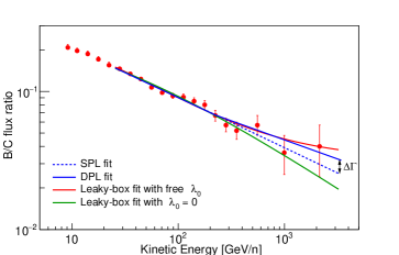
Figure 3: The CALET B/C ratio fitted to different functions. The error bars are the sum in quadrature of statistical and systematic uncertainties. The data are fitted to a DPL (solid blue line) and a SPL (dashed blue line) function in the energy interval [25, 3800] GeV$/n$. The red and green lines represent the fitted functions from a leaky-box model (Eq. (4)) with the $\lambda_{0}$ parameter left free to vary and fixed to zero, respectively.

Within the “leaky-box” (LB) approximate modeling of the particle transport in the Galaxy Obermeier et al. (2012), the B/C flux ratio can be expressed as

$$\frac{\Phi_{B}(E)}{\Phi_{C}(E)}=\frac{\lambda(E)\lambda_{B}}{\lambda(E)+\lambda_{B}}\left[\frac{1}{\lambda_{C\rightarrow B}}+\frac{\Phi_{O}(E)}{\Phi_{C}(E)}\frac{1}{\lambda_{O\rightarrow B}}\right]$$ (4)

where $\lambda_{B}$ is the interaction length of B nuclei with matter of the ISM and $\lambda_{C\rightarrow B}$ ($\lambda_{O\rightarrow B}$) is the average path length for a nucleus C (O) to spall into B. The spallation path lengths are calculated using the parametrization of the total and partial charge changing cross sections provided in Ref. Webber (1990), assuming that they are constant above a few GeV$/n$. The $\Phi_{C}(E)/\Phi_{O}(E)$ ratio is measured to be independent of energy and close to 0.91 Adriani et al. (2019). The contribution due to the spallation of heavier primary nuclei (Ne, Mg, Si, Fe) to the B flux is estimated to be $\sim$10% of the C+O flux and therefore it was not taken into account in Eq. (4). Assuming a composition of the ISM of 90% hydrogen and 10% helium, we calculate $\lambda_{B}$=9.4 g/cm², while the constant term enclosed in square brackets in Eq. (4) is 27 g/cm².

The LB model describes the diffusion of CR in the Galaxy with a mean escape path length $\lambda(E)$ which, according to presently available direct measurements, is parametrized as a power-law function of kinetic energy $E$ as follows:

$$\lambda(E)=kE^{-\delta}+\lambda_{0}$$ (5)

where $\delta$ is the diffusion coefficient spectral index. A residual path length $\lambda_{0}$ is included in the asymptotic behavior of $\lambda$. It can be interpreted as the amount of matter traversed by CR inside the acceleration region (source grammage). Fitting our B/C data to Eq. (4) (Fig. 3), the best fit values without the source grammage term ($\lambda_{0}=0$) are: $k=11.2\pm 0.5$ g/cm², $\delta=0.52\pm 0.02$ ($\chi^{2}/$d.o.f. = 13.6/13). Leaving instead $\lambda_{0}$ free to vary in the LB fit, we obtain: $k=12.0\pm 0.9$ g/cm², $\delta=0.71\pm 0.11$, $\lambda_{0}=0.95\pm 0.35$ g/cm² ($\chi^{2}/$d.o.f. = 9.6/12). These results suggest the possibility of a non-null value of the residual path length (though with a large uncertainty) which could be the cause of the apparent flattening of the B/C ratio at high energy. The best fit values of $\delta$ and $\lambda_{0}$ are compatible with the ones obtained from a combined analysis of the B/C data from earlier experiments Obermeier et al. (2012), and with the predictions of some recent theoretical works Cuoco (2021); Evoli (2019).

VI Conclusion

The CR boron spectrum has been measured by CALET up to 3.8 TeV$/n$ using 76.5 months of data collected aboard the ISS. Our observations show that, despite their different energy dependence, boron and carbon fluxes exhibit a spectral hardening occurring at about the same energy. Within the limitations of our data’s present statistical significance, the boron spectral index change is found to be slightly larger than that of carbon. This trend seems to corroborate the hypothesis that secondary CR harden more than the primaries, as recently reported by AMS-02 Aguilar et al. (2018). Interpreting our data with a LB model, we argue that the trend of the energy dependence of the B/C ratio in the TeV$/n$ region could suggest a possible presence of a residual propagation path length, compatible with the hypothesis that a fraction of secondary B nuclei can be produced near the CR source.

VII Acknowledgments

Supplemental material concerning “The Cosmic-ray Boron Flux Measured from 8.4 GeV/n to 3.8 TeV/n with the Calorimetric Electron Telescope on the International Space Station”.

VIII ADDITIONAL INFORMATION ON THE DATA ANALYSIS

Trigger. The high-energy (HE) trigger efficiency was measured directly from the flight data (FD) by using dedicated runs where in addition to HE, a low-energy (LE) trigger was active. The trigger logic is the same for both triggers (i.e. coincidence of the pulse heights of the last two pairs of IMC layers and the top TASC layer) but lower discriminator thresholds are set for the input signals in the case of the LE trigger, allowing the instrument to trigger on penetrating nuclei with $Z>2$. The ratio of the number of events counted by both triggers to those recorded by the LE trigger alone is an estimate of the HE trigger efficiency in each bin of deposited energy. The HE trigger efficiency curves as a function of the total deposited energy in the TASC ($E_{\rm{TASC}}$) are shown in Fig. S1, where they are compared with MC simulations in which both trigger modes are modeled. The FD trigger curves are in good agreement with the MC predictions, the average difference being -0.5% for B and -0.7% for C.

Charge identification. The identification of the particle charge $Z$ is based on the measurements of the ionization deposits in the CHD and IMC. The particle trajectory makes it possible to locate the CHD paddles and IMC fibers traversed by the primary particle and to determine the path length correction to the signals for the extraction of the $dE/dx$ samples. Three independent $dE/dx$ measurements are obtained, one for each CHD layer and the third one by averaging the samples (at most eight) along the track in the upper half of the IMC, summing up the signals of the crossed fiber in each layer and its two neighbors. In order to suppress the contribution of possible signals of secondary tracks wrongly associated to the track of the primary nucleus, only $dE/dx$ signals larger than 1.5 MeV/mm (corresponding to the energy released in a fiber by 10 MIPs (Minimum Ionizing Particles)) are used in the mean calculation.
Calibration curves of $dE/dx$ are built by fitting FD subsets for each nuclear species to a function of $Z^{2}$ by using a “halo” model Marrocchesi et al. (2011), in which $dE/dx$ is parametrized as the sum of two contributions (“core” and “halo”, respectively)

$$\frac{dE}{dx}=\frac{A(1-f_{h})\alpha Z^{2}}{1+B_{S}(1-f_{h})\alpha Z^{2}+C_{S}\alpha^{2}Z^{4}}+Af_{h}\alpha Z^{2}$$ (S1)

where the parameter $f_{h}$ represents the fraction of energy deposited in the halo; $B_{S}$ and $C_{S}$ model the strength of the scintillation quenching; $A$ is an overall normalization constant; and $\alpha$ is close to 2 MeV g^-1 cm² for a plastic scintillator. The parameters are extracted from the fits separately for the CHDX, CHDY and IMC. These three calibration curves are then used to reconstruct three charge values ($Z_{\rm{CHDX}}$, $Z_{\rm{CHDY}}$, $Z_{\rm{IMC}}$) from the measured $dE/dx$ yields on an event-by-event basis. For high-energy showers, the charge peaks are corrected for a systematic shift to higher values (up to 0.15 $e$) with respect to the nominal charge positions, due to the large amount of shower particle tracks backscattered from the TASC whose signals add up to the primary particle ionization signal. The resulting distribution of the reconstructed charge ($Z_{\rm{CHD}}$) combining $Z_{\rm{CHDX}}$ and $Z_{\rm{CHDY}}$ is shown in Fig. S2(a). B and C candidates are selected by applying a window cut of half-width 0.45 centered on the nominal charge values ($Z=5,6$). Events with C nuclei undergoing a charge-changing nuclear interaction at the top of the IMC are clearly visible in the tail of the C drop-shaped distribution extending to lower $Z_{IMC}$ values in Fig. S2(b). They are removed by requiring consistency between the CHD and IMC charges ($|Z_{\rm{CHD}}-Z_{\rm{IMC}}|<1$), and among the individual charge values measured in the four upper pairs of adjacent fiber layers.

Track width. A clustering algorithm is applied to the fibers being hit in the IMC before track finding and fitting. In each IMC layer, neighboring fibers with an energy deposit $>$0.3 MIPs are clustered around the fibers with larger signals. The position of each cluster is computed as the center-of-gravity (COG) of its fibers. The cluster positions are taken as candidate track points for the combinatorial Kalman filter algorithm Maestro and Mori (2017) which is used to identify the clusters associated to the primary particle track and to reconstruct its direction and entrance point at the top of the instrument. In each layer $l$, we define the track width as

$$\rm{TW}_{l}=\frac{\sum\limits_{j=m-3}^{m+3}E_{l,j}-\sum\limits_{j=m-1}^{m+1}E_{l,j}}{Z_{l}^{2}}$$ (S2)

where $E_{l,j}$ is the energy deposit in the fiber $j$ of the layer $l$, $m$ is the index of the fiber with the maximum signal in the cluster crossed by the primary particle track, and the numerator represents the difference between the total energy deposited in the 7 central fibers of the cluster and the cluster core, made of 3 fibers. $Z_{l}$ is the charge in the layer $l$ which is calculated by using the signals of the 5 central fibers in the cluster crossed by the track. The total track width is then defined as

$$\rm{TW}=\frac{1}{6}\sum\limits_{l=1}^{6}\rm{TW}_{l}$$ (S3)

where the sum is limited to the first eight IMC layers from the top excluding the two layers with maximum and minimum $Z_{l}$, respectively.

The $\rm{TW}$ of interacting events at the top of the instrument is wider than that of penetrating nuclei, due to the angular spread of secondary particles produced in the interaction and their lower specific ionization compared to that of the primary particle. In Fig. S3, a sample of B events selected in FD by means of the CHD only (i.e. without the IMC consistency cuts described above) is compared with the distributions obtained from MC simulations of B and other nuclei, applying the same selections as for FD. It can be noticed that B nuclei traversing CHD and the top of the IMC without interacting show a peak at low $\rm{TW}$ values (red filled histogram), while the broad distribution at large $\rm{TW}$ values is due to the interaction of background particles (mainly protons, He, C) misidentified as boron (blue filled histogram). A cut on $\rm{TW}<0.18$ is applied to select penetrating B events and reject both early interacting B nuclei (the right-hand tail in the red filled histogram) and the background from other nuclear species.

Studying $\rm{TW}$ distributions similar to the ones shown in Fig. S3 but obtained by applying also the IMC consistency cuts, a residual background contamination can be computed as the fraction of nuclei misidentified as B and not rejected by the $\rm{TW}$ cut, compared to the number of selected B events in different intervals of $E_{\rm{TASC}}$. This contamination fraction is $\sim 1\%$ for $E_{\rm TASC}<10^{2}$ GeV and grows logarithmically for $E_{\rm TASC}>10^{2}$ GeV, approaching $\sim 7\%$ at 1.5 TeV. The estimated $E_{\rm{TASC}}$ distribution of the background in the final B sample is shown in Fig. S4 as a blue-filled histogram. It is subtracted from the B distribution in FD (red-filled histogram) before the application of the unfolding procedure.

Selection efficiency. The efficiency of the complete selection procedure of B and C nuclei, estimated from MC and including trigger, tracking, charge identification and $\rm{TW}$ efficiencies, is shown as a function of the kinetic energy per nucleon in Fig. S5.

Systematic uncertainties. The flux systematic relative errors stemming from several sources, including HE trigger efficiency, charge identification, MC simulations, energy scale, energy unfolding, background contamination, and live time are shown in Fig. S6 as a function of the kinetic energy per nucleon. The dominant source of uncertainty in the flux derives from the different predictions of the energy response matrix by simulations based on EPICS and Geant4. Energy-independent systematic uncertainties affecting the flux normalization include live time (3.4%), long-term stability of charge calibration (0.5%), energy scale calibration (3%), and assumption of the B isotopic composition (1.7%). With the exception of the latter, the other energy-independent systematic uncertainties cancel out completely in the B/C ratio.

Additional systematic effects that have been studied extensively are related to the particle interactions in the materials of the instrument. Primary particles cross a 2 mm-think Al panel covering the top of the instrument, before reaching the CHD. The probability of interactions of B and C nuclei in this panel is $\lesssim$1%. This effect is taken into account in the flux calculation.
CR nuclei traverse several materials in the IMC, mainly composed of CFRP (Carbon Fiber Reinforced Polymer), aluminum and tungsten. Possible uncertainties in the inelastic cross sections in MC simulations or discrepancies in the material description might affect the flux normalization. We have checked that hadronic interactions are well simulated in the detector, by measuring the survival probabilities of C nuclei at different depths in the IMC. The survival probabilities are in agreement with MC prediction within $<$1% as shown in Fig. S7.

Several studies were performed to check the stability of the detector performance. Day-by-day calibrations of the detector channels are performed by using penetrating protons and He particles selected by a dedicated trigger mode. This ensures that the CHD and IMC charge measurements are stable over time at the level of 0.5%.
To investigate the uncertainty in the definition of the acceptance, restricted acceptance (up to 20% of the nominal one) regions were also studied. The corresponding fluxes are consistent within statistical fluctuations.
To investigate possible time-dependent effects in the energy scale of the TASC, we have compared C flux measurements obtained with subsets of data taken in different periods of time. We have chosen for comparison an energy interval between 30 GeV/$n$ and 300 GeV/$n$, to exclude the low-energy region where the flux is affected by solar modulation and the high-energy region where statistical fluctuations are relevant. In this energy interval, the fluxes in different time periods turned out to be in agreement at a level consistent with the energy scale calibration error (3%).

Energy spectra. The CALET energy spectra of B and C and the B/C flux ratio, together with a compilation of the available data, are shown in Fig. S8, which is an enlarged version of Fig. 2 in the main body of the paper. In tables 1 and 2, the B and C differential fluxes in different energy intervals are reported with the separate contributions to the flux error of the statistical uncertainties, the systematic uncertainties in normalization, and energy dependent systematic uncertainties. The data of the B/C flux ratio are reported in table 3.

Figure S1: HE trigger efficiency as a function of the deposited energy in the TASC for B (a) and C (b) as derived from flight data (FD) (black dots) and Monte Carlo (MC) (red curves). The difference between FD and MC efficiencies is within $\pm 2\%$ over the whole energy range, as shown by the red dotted lines in the bottom plots of panels (a) and (b). The average difference is -0.5% for B and -0.7% for C, as indicated by the blue lines.

Figure S2: (a) Charge distribution measured in the energy interval 100 $<E_{\rm{TASC}}/\text{GeV}<$ 215 by the combined CHD layers (FD, black dots) compared to MC simulations. Events are selected by requiring a measured charge in IMC consistent with $Z_{\rm CHD}$ and a track width $\rm{TW}<0.18$ (Fig. S3). (b) Charge correlation between $Z_{\rm{IMC}}$ and $Z_{\rm{CHD}}$ in a sample of FD selected without applying the consistency cuts between CHD and IMC or the $\rm{TW}$ cut.

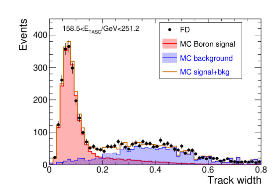
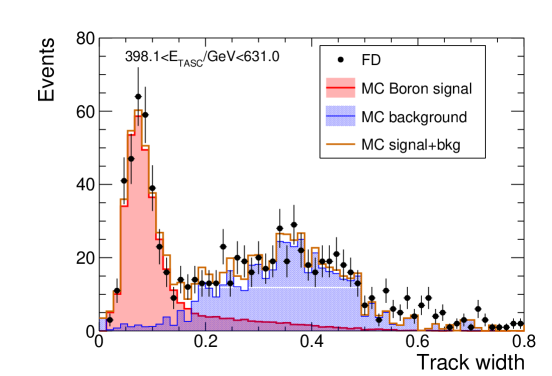
Figure S3: Distributions of the track width ($\rm{TW}$) variable in two different intervals of $E_{\rm TASC}$. The black dots represent a sample of B events selected in FD by means of the CHD only. MC distributions of B and other background nuclei (mainly proton, He, C) are obtained with the same selections used for FD.

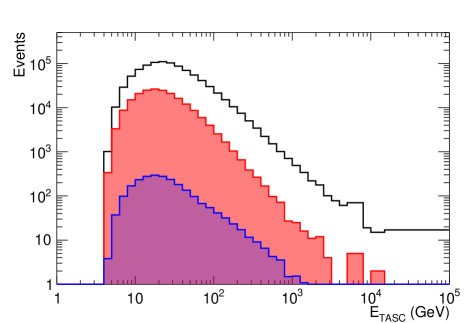
Figure S4: Distribution of total deposited energy in the TASC for the final selection of carbon (black histogram) and boron (red histogram) candidates in FD. The blue-filled histogram represents the background contamination subtracted from the B sample for the flux measurement.

Figure S5: Total selection efficiency for B (red dots) and C (black dots) estimated with MC simulations.

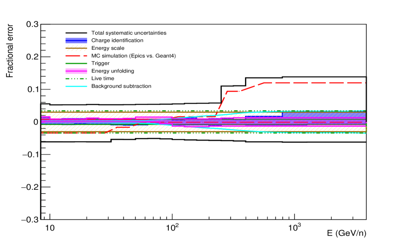
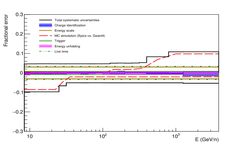
Figure S6: Energy dependence of systematic uncertainties (relative errors) for B (a) and C (b). The band within the black lines shows the sum in quadrature of all the sources of systematics. A detailed breakdown of systematic errors stemming from charge identification, HE trigger, MC simulations, energy scale, energy unfolding, background contamination, live time is shown.

Figure S7: Survival probability as a function of the material thickness traversed by C nuclei in the IMC as derived from FD (black triangles) and MC (red circles). The survival probabilities are calculated in FD by dividing the number of events selected as C in the first six double layers of scintillating fibers in the IMC by the number of C events selected with the CHD. The material thickness is expressed in units of proton interaction length $\lambda_{I}$ and it is measured from the bottom of the CHD. The double fiber layers are preceded by 0.2 $X_{0}$-thick W plates (except the first pair), Al honeycomb panels and CFRP supporting structures. In the bottom panel, the blue line represents a constant value fitted to the ratio between MC and FD survival probabilities. The fitted value is $1.006\pm 0.006$.

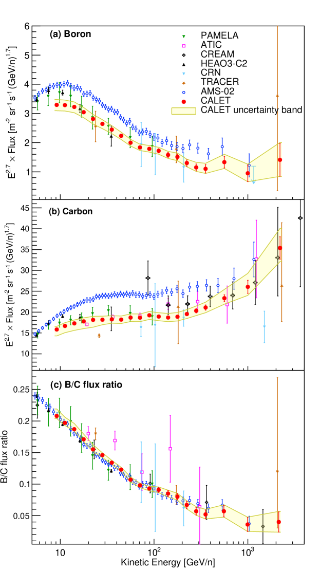
Figure S8: CALET (a) boron and (b) carbon flux (multiplied by $E^{2.7}$) and (c) ratio of boron to carbon, as a function of kinetic energy $E$. Error bars of CALET data (red) represent the statistical uncertainty only, while the yellow band indicates the quadratic sum of statistical and systematic errors. Also plotted are other direct measurements Engelmann et al. (1990); Swordy et al. (1990); Ahn et al. (2008); Obermeier et al. (2012); Adriani et al. (2014); Aguilar et al. (2021b, 2018); Panov et al. (2009); Ahn et al. (2009).

Table 1: Table of CALET boron spectrum. The first, second and third errors in the flux represent the statistical uncertainties, systematic uncertainties in normalization, and energy dependent systematic uncertainties, respectively.

Energy Bin [GeV$/n$]	Flux [m-2sr-1s-1(GeV$/n$)-1]
8.4–10.0	$(8.313\,\pm 0.045\,\pm 0.405\,_{-0.307}^{+0.221})\times 10^{-3}$
10.0–12.6	$(4.811\,\pm 0.029\,\pm 0.234\,_{-0.178}^{+0.092})\times 10^{-3}$
12.6–15.8	$(2.535\,\pm 0.018\,\pm 0.123\,_{-0.094}^{+0.051})\times 10^{-3}$
15.8–20.0	$(1.285\,\pm 0.011\,\pm 0.063\,_{-0.047}^{+0.026})\times 10^{-3}$
20.0–25.1	$(6.379\,\pm 0.065\,\pm 0.311\,_{-0.236}^{+0.142})\times 10^{-4}$
25.1–31.6	$(3.219\,\pm 0.039\,\pm 0.157\,_{-0.119}^{+0.065})\times 10^{-4}$
31.6–39.8	$(1.600\,\pm 0.024\,\pm 0.078\,_{-0.037}^{+0.033})\times 10^{-4}$
39.8–50.1	$(7.846\,\pm 0.142\,\pm 0.382\,_{-0.182}^{+0.164})\times 10^{-5}$
50.1–63.1	$(3.768\,\pm 0.085\,\pm 0.183\,_{-0.060}^{+0.087})\times 10^{-5}$
63.1–79.4	$(1.859\,\pm 0.052\,\pm 0.091\,_{-0.028}^{+0.044})\times 10^{-5}$
79.4–100.0	$(9.723\,\pm 0.335\,\pm 0.473\,_{-0.176}^{+0.237})\times 10^{-6}$
100.0–125.9	$(5.026\,\pm 0.210\,\pm 0.245\,_{-0.118}^{+0.133})\times 10^{-6}$
125.9–158.5	$(2.476\,\pm 0.130\,\pm 0.121\,_{-0.065}^{+0.073})\times 10^{-6}$
158.5–199.5	$(1.273\,\pm 0.083\,\pm 0.062\,_{-0.036}^{+0.038})\times 10^{-6}$
199.5–251.2	$(5.889\,\pm 0.483\,\pm 0.287\,_{-0.172}^{+0.186})\times 10^{-7}$
251.2–316.2	$(2.795\,\pm 0.290\,\pm 0.136\,_{-0.085}^{+0.276})\times 10^{-7}$
316.2–398.1	$(1.438\,\pm 0.189\,\pm 0.070\,_{-0.047}^{+0.143})\times 10^{-7}$
398.1–794.3	$(5.010\,\pm 0.753\,\pm 0.244\,_{-0.186}^{+0.633})\times 10^{-8}$
794.3–1258.9	$(7.553\,\pm 2.253\,\pm 0.368\,_{-0.292}^{+0.978})\times 10^{-9}$
1258.9–3860.5	$(1.328\,\pm 0.528\,\pm 0.065\,_{-0.051}^{+0.172})\times 10^{-9}$

Table 2: Table of CALET carbon spectrum. The first, second and third errors in the flux represent the statistical uncertainties, systematic uncertainties in normalization, and energy dependent systematic uncertainties, respectively.

Energy Bin [GeV$/n$]	Flux [m-2sr-1s-1(GeV$/n$)-1]
8.4–10.0	$(3.990\,\pm 0.010\,\pm 0.182\,_{-0.343}^{+0.037})\times 10^{-2}$
10.0–12.6	$(2.440\,\pm 0.006\,\pm 0.111\,_{-0.208}^{+0.025})\times 10^{-2}$
12.6–15.8	$(1.358\,\pm 0.004\,\pm 0.062\,_{-0.116}^{+0.016})\times 10^{-2}$
15.8–20.0	$(7.496\,\pm 0.026\,\pm 0.342\,_{-0.641}^{+0.088})\times 10^{-3}$
20.0–25.1	$(4.108\,\pm 0.016\,\pm 0.187\,_{-0.351}^{+0.044})\times 10^{-3}$
25.1–31.6	$(2.211\,\pm 0.010\,\pm 0.101\,_{-0.106}^{+0.023})\times 10^{-3}$
31.6–39.8	$(1.193\,\pm 0.006\,\pm 0.054\,_{-0.026}^{+0.013})\times 10^{-3}$
39.8–50.1	$(6.385\,\pm 0.040\,\pm 0.291\,_{-0.138}^{+0.069})\times 10^{-4}$
50.1–63.1	$(3.520\,\pm 0.025\,\pm 0.161\,_{-0.077}^{+0.038})\times 10^{-4}$
63.1–79.4	$(1.888\,\pm 0.016\,\pm 0.086\,_{-0.041}^{+0.020})\times 10^{-4}$
79.4–100.0	$(1.045\,\pm 0.011\,\pm 0.048\,_{-0.023}^{+0.011})\times 10^{-4}$
100.0–125.9	$(5.523\,\pm 0.067\,\pm 0.252\,_{-0.123}^{+0.063})\times 10^{-5}$
125.9–158.5	$(2.930\,\pm 0.043\,\pm 0.134\,_{-0.065}^{+0.062})\times 10^{-5}$
158.5–199.5	$(1.589\,\pm 0.028\,\pm 0.073\,_{-0.035}^{+0.035})\times 10^{-5}$
199.5–251.2	$(8.830\,\pm 0.186\,\pm 0.403\,_{-0.196}^{+0.185})\times 10^{-6}$
251.2–316.2	$(4.931\,\pm 0.122\,\pm 0.225\,_{-0.109}^{+0.112})\times 10^{-6}$
316.2–398.1	$(2.750\,\pm 0.082\,\pm 0.125\,_{-0.061}^{+0.074})\times 10^{-6}$
398.1–794.3	$(8.770\,\pm 0.305\,\pm 0.400\,_{-0.196}^{+0.610})\times 10^{-7}$
794.3–1258.9	$(2.070\,\pm 0.124\,\pm 0.094\,_{-0.046}^{+0.204})\times 10^{-7}$
1258.9–3860.5	$(3.325\,\pm 0.252\,\pm 0.152\,_{-0.089}^{+0.328})\times 10^{-8}$

Table 3: Table of CALET boron to carbon flux ratio. The first and second errors represent the statistical uncertainties and systematic uncertainties, respectively.

Energy Bin [GeV$/n$]	B/C
8.4–10.0	$0.208\,\pm 0.001\,_{-0.004}^{+0.011}$
10.0–12.6	$0.197\,\pm 0.001\,_{-0.004}^{+0.009}$
12.6–15.8	$0.187\,\pm 0.001\,_{-0.003}^{+0.009}$
15.8–20.0	$0.171\,\pm 0.002\,_{-0.003}^{+0.008}$
20.0–25.1	$0.155\,\pm 0.002\,_{-0.003}^{+0.007}$
25.1–31.6	$0.146\,\pm 0.002\,_{-0.003}^{+0.003}$
31.6–39.8	$0.134\,\pm 0.002\,_{-0.002}^{+0.003}$
39.8–50.1	$0.123\,\pm 0.002\,_{-0.002}^{+0.003}$
50.1–63.1	$0.107\,\pm 0.003\,_{-0.002}^{+0.003}$
63.1–79.4	$0.098\,\pm 0.003\,_{-0.002}^{+0.002}$
79.4–100.0	$0.093\,\pm 0.003\,_{-0.002}^{+0.002}$
100.0–125.9	$0.091\,\pm 0.004\,_{-0.002}^{+0.002}$
125.9–158.5	$0.085\,\pm 0.005\,_{-0.002}^{+0.002}$
158.5–199.5	$0.080\,\pm 0.005\,_{-0.002}^{+0.002}$
199.5–251.2	$0.067\,\pm 0.006\,_{-0.002}^{+0.002}$
251.2–316.2	$0.057\,\pm 0.006\,_{-0.002}^{+0.004}$
316.2–398.1	$0.052\,\pm 0.007\,_{-0.002}^{+0.004}$
398.1–794.3	$0.057\,\pm 0.009\,_{-0.002}^{+0.005}$
794.3–1258.9	$0.036\,\pm 0.011\,_{-0.001}^{+0.004}$
1258.9–3860.5	$0.040\,\pm 0.016\,_{-0.002}^{+0.005}$