Octonionic Calabi-Yau theorem.

Abstract

On a certain class of 16-dimensional manifolds a new class of Riemannian metrics, called octonionic Kähler, is introduced and studied. It is an octonionic analogue of Kähler metrics on complex manifolds and of HKT-metrics of hypercomplex manifolds. Then for this class of metrics an octonionic version of the Monge-Ampère equation is introduced and solved under appropriate assumptions. The latter result is an octonionic version of the Calabi-Yau theorem from Kähler geometry.

1 Introduction.

1. Real and complex Monge-Ampère (MA) equations play a central role in several areas of analysis and geometry. In particular, the celebrated Calabi-Yau theorem [58] establishes existence of Ricci flat Kähler metrics on compact Kähler manifolds reducing the problem to solving a complex MA equation. This result is a powerful analytic tool to study geometry and topology of compact Kähler manifolds.

2. There were several attempts to generalize the notion of MA equation and of plurisubharmonic function to a few other contexts. Namely, the Calabi-Yau theorem was successfully extended to the more general class of compact Hermitian manifolds by Tosatti-Weinkove [54] in full generality and previously by Cherrier [20] in special cases.

   Furthermore, the first author [3] introduced and studied the quaternionic MA operator and the class of quaternionic plurisubharmonic (qpsh) functions on the flat quaternionic space $\mathbb{H}^{n}$. Later he introduced and solved, under appropriate assumptions, the Dirichlet problem for quaternionic MA equation in [4]. The latter problem was solved under weaker assumptions by Zhu [59] and Kolodziej-Sroka [52].

   M. Verbitsky and the first author [12] extended the definition of the quaternionic MA operator and the class of qpsh functions to the broader class of hypercomplex manifold; then the first author [8] extended them to even broader class of quaternionic manifolds. M. Verbitsky and the first author [13] introduced a quaternionic version of the Calabi problem. So far this problem is open in full generality, but it was proven in a few special cases, see [9], [26], [21]. Some relevant a priori estimates were obtained in [13], [10], [11], [51].

   A number of results in quaternionic pluripotential theory were obtained in [57], [55], [56].

3. The MA operator and a class of plurisubharmonic functions in two octonionic variables were introduced by the first author in [7], where also a few properties of them were established and an application to valuations on convex sets was given.

4. At the same time there is a parallel development by Harvey and Lawson, e.g. [31], [32], [33], [34]. The notion of plurisubharmonic function is developed in great generality, as well as the theory of homogeneous MA equation. Being specialized to the quaternionic situation, this theory has an overlap with some of the results mentioned above.

5. Let us describe the main results of this paper.

   As mentioned above, the MA operator in two octonionic variables was introduced by the first author in [7]. Based on this operator, the present paper introduces and studies the octonionic MA equation analogous to the Calabi problem in Kähler geometry.

   The MA equation is stated for a special class of 16-dimensional manifolds with a kind of octonionic structure. We call such manifolds $GL_{2}(\mathbb{O})$-manifolds, they are introduced in Section 8. Basic examples of such manifolds are torii $\mathbb{O}^{2}/\Lambda$, where $\mathbb{O}^{2}\simeq\mathbb{R}^{16}$ is the octonionic plane, and $\Lambda\subset\mathbb{O}^{2}$ is a lattice.

   Furthermore in Section 9 we introduce on any $GL_{2}(\mathbb{O})$-manifold a class of Riemannian metrics which are octonionic analogues of Kähler metrics. We call them octonionic Kähler metrics. In local coordinates, i.e. on $\mathbb{O}^{2}$, such metrics are characterized by two conditions. First, the restriction of each such metric on any (right) octonionic line is proportional to the standard Euclidean metric on $\mathbb{O}^{2}\simeq\mathbb{R}^{16}$. Second, such metrics satisfy a system of linear first order PDEs (see (9.1)) analogous to the closeness of Kähler form on a complex manifold. We also prove an analogue of the local $dd^{c}$-lemma from complex analysis (see Theorem 9.2): locally any such metric can be given by a smooth potential $u$, i.e. the metric can be identified with the octonionic Hessian of $u$. The converse is also true provided the Hessian of $u$ is pointwise positive definite.

   Next we introduce an octonionic MA equation on a $GL_{2}(\mathbb{O})$-manifold $M$. Let $G_{0}$ be an octonionic Kähler ($C^{\infty}$-smooth) metric; in local coordinates it can be identified with a positive definite octonionic Hermitian matrix. Let $f\colon M\longrightarrow\mathbb{R}$ be a $C^{\infty}$-smooth function. Consider the equation which in local coordinates reads

   $$\det(G_{0}+Hess_{\mathbb{O}}(\phi))=e^{f}\det(G_{0}),$$ (1.1)

   where $Hess_{\mathbb{O}}$ is the octonionic Hessian (see Section 4 for the precise definition), $\det$ is the determinant of octonionic Hermitian $2\times 2$ matrices (see (5.10)). The main result of this paper, Theorem 11.3, says that on the subclass of compact connected so called $Spin(9)$-manifolds (example: tori $\mathbb{O}^{2}/\Lambda$ where $\Lambda\subset\mathbb{O}^{2}$ is a lattice) there exists a $C^{\infty}$-smooth solution $\phi$ of (1.1) if and only if the function $f$ satisfies the normalization condition

   $$\int_{M}(e^{f}-1)\det(G_{0})\cdot\Theta=0,$$

   where $\Theta$ is a parallel non-vanishing 3/4-density on $M$ (it always exists on $Spin(9)$-manifolds and is unique up to multiplication by a constant).

6. The class of metrics on $GL_{2}(\mathbb{O})$-manifolds we mentioned is analogous not only to Kähler metrics on complex manifolds, but also to Hessian metrics on affine manifolds [19], and to HKT-metrics on hypercomplex manifolds [36], [28]. Our main result on the solvability of the MA equation is analogous to and is motivated by the Calabi-Yau theorem [58] for Kähler manifolds. Also it is analogous to the Cheng-Yau theorem [19] for Hessian manifolds, and to the similar conjecture on quaternionic MA equation on HKT-manifolds due to M. Verbitsky and the author [13] which has been proven so far in a few special cases mentioned above.

7. In literature there are quite a few investigations of geometric structures related to octonions. Thus Gibbons, Papadopoulos, and Stelle [24] introduced a class of Octonionic Kähler with Torsion metrics on $8k$-dimensional manifolds in connection with black hole moduli spaces.

   Friedrich [23] introduced the notion of nearly parallel $Spin(9)$-structure on 16-manifolds whose structure group is reduced to $Spin(9)$. The role of $Spin(9)$ in octonionic geometry is reviewed by Parton and Piccinni [47] (see also [38]).

   Very recently Kotrbatý and Wannerer [39] described the multiplicative structure on $Spin(9)$-invariant valuations on convex sets on $\mathbb{O}^{2}$ and gave applications to integral geometry.

8. Acknowledgements. We thank F. Nazarov and M. Sodin for useful discussions and G. Grantcharov, G. Papadopoulos, I. Soprunov, and A. Swann for supplying us with some references.

2 Algebra of octonions.

1. The octonions $\mathbb{O}$ form an 8-dimensional algebra over the reals $\mathbb{R}$ which is neither associative nor commutative. The product on $\mathbb{O}$ can be described as follows. $\mathbb{O}$ has a basis $e_{0},e_{1},\dots,e_{7}$ over $\mathbb{R}$ where $e_{0}=1$ is the unit, and the product of basis elements is given by the following multiplication table:

   $$\begin{array}[]{c|c|c|c|c|c|c|c|}&e_{1}&e_{2}&e_{3}&e_{4}&e_{5}&e_{6}&e_{7}\\ \hline\cr e_{1}&-1&e_{4}&e_{7}&-e_{2}&e_{6}&-e_{5}&-e_{3}\\ \hline\cr e_{2}&-e_{4}&-1&e_{5}&e_{1}&-e_{3}&e_{7}&-e_{6}\\ \hline\cr e_{3}&-e_{7}&-e_{5}&-1&e_{6}&e_{2}&-e_{4}&e_{1}\\ \hline\cr e_{4}&e_{2}&-e_{1}&-e_{6}&-1&e_{7}&e_{3}&-e_{5}\\ \hline\cr e_{5}&-e_{6}&e_{3}&-e_{2}&-e_{7}&-1&e_{1}&e_{4}\\ \hline\cr e_{6}&e_{5}&-e_{7}&e_{4}&-e_{3}&-e_{1}&-1&e_{2}\\ \hline\cr e_{7}&e_{3}&e_{6}&-e_{1}&e_{5}&-e_{4}&-e_{2}&-1\\ \hline\cr\end{array}$$

2. There is also an easier alternative way to reproduce the product rule using the so called Fano plane (see Figure 1 below). In Figure 1 each pair of distinct points lies in a unique line (the circle is also considered to be a line). Each line contains exactly three points, and these points are cyclically oriented. If $e_{i},e_{j},e_{k}$ are cyclically oriented in this way then

   $$e_{i}e_{j}=-e_{j}e_{i}=e_{k}.$$

   We have to add two more rules:

   $\bullet$ $e_{0}=1$ is the identity element;

   $\bullet$ $e_{i}^{2}=-1$ for $i>0$.

   All these rules define uniquely the algebra structure of $\mathbb{O}$. The center of $\mathbb{O}$ is equal to $\mathbb{R}$.

   

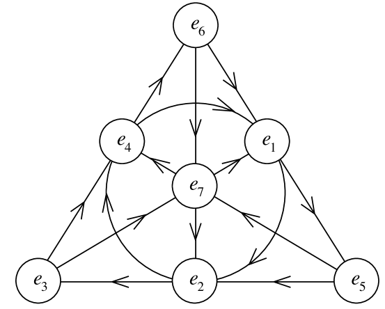
   Figure 1: Fano plane, the figure is taken from [16]

3. Every octonion $q\in\mathbb{O}$ can be written uniquely in the form

   $$q=\sum_{i=0}^{7}x_{i}e_{i}$$

   where $x_{i}\in\mathbb{R}$. The summand $x_{0}e_{0}=x_{0}$ is called the real part of $q$ and is denoted by $Re(q)$.

   One defines the octonionic conjugate of $q$ by

   $$\bar{q}:=x_{0}-\sum_{i=1}^{7}x_{i}e_{i}.$$

   It is well known that the conjugation is an anti-involution of $\mathbb{O}$:

   $$\overline{\overline{q}}=q,\,\overline{a+b}=\bar{a}+\bar{b},\,\overline{ab}=\bar{b}\bar{a}.$$

   Let us define a norm on $\mathbb{O}$ by $|q|:=\sqrt{q\bar{q}}$. Then $|\cdot|$ is a multiplicative norm on $\mathbb{O}$: $|ab|=|a||b|$. The square of the norm $|\cdot|^{2}$ is a positive definite quadratic form. Its polarization is a positive definite scalar product $<\cdot,\cdot>$ on $\mathbb{O}$ which is given explicitly by

   $$<x,y>=Re(x\bar{y}).$$

   Furthermore $\mathbb{O}$ is a division algebra: any $q\neq 0$ has a unique inverse $q^{-1}$ such that $qq^{-1}=q^{-1}q=1$. In fact

   $$q^{-1}=|q|^{-2}\bar{q}.$$

4. We denote by $\mathbb{H}$ the usual quaternions. It is associative division algebra. We will fix once and for all an imbedding of algebras $\mathbb{H}\subset\mathbb{O}$. Let us denote by $i,j\in\mathbb{H}$ the usual quaternionic units, and $k=ij$. Then $i,j,k$ are pairwise orthogonal with respect to the scalar product $<\cdot,\cdot>$. Let us fix once and for all an octonionic unit $l\in\mathbb{O},l^{2}=-1$ which is orthogonal to $i,j,k$. Then $l$ anti-commutes with $i,j,k$. Every element $q\in\mathbb{O}$ can be written uniquely in the form

   $$q=x+yl\mbox{ with }x,y\in\mathbb{H}.$$

   The multiplication of two such octonions is given by the formula

   $$(x+yl)(w+zl)=(xw-\bar{z}y)+(zx+y\bar{w})l$$ (2.1)

   where $x,y,w,z\in\mathbb{H}$.

5. We have the following weak forms of the associativity in octonions. A proof can be found in [7], Lemma 1.1.1.

   2.1 Lemma.

   Let $a,b,c\in\mathbb{O}$. Then

   (i) $Re((ab)c)=Re(a(bc))$ (this real number will be denoted by $Re(abc)$).

   (ii) $a(bc)+\bar{b}(\bar{a}c)=(ab+\bar{b}\bar{a})c$.

   (iii) $(ca)b+(c\bar{b})\bar{a}=c(ab+\bar{b}\bar{a})$.

   (iv) Any subalgebra of $\mathbb{O}$ generated by any two elements and their conjugates is associative. It is always isomorphic either to $\mathbb{R}$, $\mathbb{C}$, or $\mathbb{H}$.

   (v) $Re((\bar{a}b)(ca))=|a|^{2}Re(bc).$

   The following identities are called Moufang identities (see e.g. [48]).

   2.2 Lemma.

   Let $x,y,z\in\mathbb{O}$. Then

   $$(zx)(yz)=z((xy)z)=(z(xy))z.$$

   Polarizing the Moufang identities we immediately get a corollary.

   2.3 Corollary.

   Let $x,y,z_{1},z_{2}\in\mathbb{O}$. Then

   $$(z_{1}x)(yz_{2})+(z_{2}x)(yz_{1})=z_{1}((xy)z_{2})+z_{2}((xy)z_{1})=(z_{1}(xy))z_{2}+(z_{2}(xy))z_{1}.$$

3 Octonionic projective line $\mathbb{O}\mathbb{P}^{1}$.

1. The results of this section are well known and elementary, we provide them for completeness of presentation.

   3.1 Definition.

   An octonionic (right) line in $\mathbb{O}^{2}$ is a real 8-dimensional subspace $L\subset\mathbb{O}^{2}$ either of the form $\{(q,aq)|q\in\mathbb{O}\}$ with arbitrary $a\in\mathbb{O}$, or of the form $\{(0,q)|q\in\mathbb{O}\}$.

   The latter option is considered as the line at infinity. The set of all octonionic lines is denoted by $\mathbb{O}\mathbb{P}^{1}$. It is easy to see that it is a compact subset of the Grassmannian of 8-dimensional linear subspaces of $\mathbb{R}^{16}$. Moreover it is a smooth submanifold diffeomorphic to the 8-sphere $\SS^{8}$: the line at infinity corresponds to the pole of this sphere, and the rest is parameterized by octonions $a\in\mathbb{O}$ is diffeomorphic to $\mathbb{R}^{8}$.

2. Let us summarize a few other basic and well known properties of $\mathbb{O}\mathbb{P}^{1}$.

   3.2 Lemma.

   (i) For any $a\in\mathbb{O}$ the set $\{(aq,q)|q\in\mathbb{O}\}$ is also an octonionic line.
   (ii) Any two octonionic lines either intersect trivially or coincide.
   (iii) For any non-zero vector $\xi\in\mathbb{O}^{2}$ there is a unique octonionic line containing $\xi$. We call it the line spanned by $\xi$.
   (iv) Let $\xi,\eta\in\mathbb{O}$ be two vectors of norm one. The lines spanned by these vectors are equal if and only if one has for the $2\times 2$-matrices

   $$\xi\cdot\xi^{*}=\eta\cdot\eta^{*}.$$

   In this case we write $\xi\sim\eta$.

   The proof of this lemma is elementary and straightforward.

4 Octonionic Hessian.

In this section we remind the octonionic Hessian introduced in [7]. For $i=1,2$ write

$$q_{i}=\sum_{a=0}^{7}x_{i}^{a}e_{a}\mbox{ with }x_{i}^{a}\in\mathbb{R}.$$

Let $F\colon\mathbb{O}^{2}\longrightarrow\mathbb{O}$ be a sufficiently smooth function. Define for $i,j=1,2$

$$\frac{\partial F}{\partial\bar{q}_{i}}:=\sum_{a=0}^{7}e_{a}\frac{\partial F}{\partial x_{i}^{a}},$$

$$\frac{\partial F}{\partial q_{j}}:=\sum_{a=0}^{7}\frac{\partial F}{\partial x_{j}^{a}}\bar{e}_{a}.$$

In general the operators $\frac{\partial}{\partial\bar{q}_{i}}$ and $\frac{\partial}{\partial q_{j}}$ do not commute. However, they do commute when applied to real valued functions.

Let $f\colon\mathbb{O}^{2}\longrightarrow\mathbb{R}$ be a $C^{2}$-smooth real valued function. Define its octonionic Hessian by

$$Hess_{\mathbb{O}}(f):=\left(\frac{\partial^{2}f}{\partial\bar{q}_{i}\partial q_{j}}\right)_{i,j=1,2},$$ (4.1)

where the operators $\frac{\partial}{\partial\bar{q}_{i}}$ and $\frac{\partial}{\partial q_{j}}$ are applied in either order. Then $Hess_{\mathbb{O}}(f)$ is an octonionic Hermitian $2\times 2$ matrix.

5 Octonionic linear algebra.

1. Let us denote

   $$\mathbb{O}^{m}:=\{(q_{1},\dots,q_{m})|\,q_{i}\in\mathbb{O}\}.$$

   For $\xi=(q_{1},\dots,q_{m})\in\mathbb{O}^{m}$, $x\in\mathbb{O}$ we will denote by $\xi\cdot x$ the $m$-tuple $(q_{1}x,\dots,q_{m}x)\in\mathbb{O}^{m}$. Notice that usually we will write elements of $\mathbb{O}^{m}$ as $m$-columns rather than rows.

   Let us denote by ${\cal H}_{n}(\mathbb{R})$ the space of real symmetric $(n\times n)$-matrices. The space ${\cal H}_{n}(\mathbb{R})$ is naturally identified with the space of real valued quadratic forms on $\mathbb{R}^{n}$.

   Let us denote by ${\cal H}_{m}(\mathbb{O})$ the space of octonionic Hermitian $(m\times m)$-matrices. By definition, an $(m\times m)$-matrix $A=(a_{ij})$ with octonionic entries is called Hermitian if $a_{ij}=\overline{a_{ji}}$ for any $i,j$. For a matrix $A=(a_{ij})$ denote also $A^{*}:=(\overline{a_{ji}})$. In what follows we will be only interested in $2\times 2$ octonionic Hermitian matrices. In this case we have the following explicit description of such matrices. Namely,

   $${\cal H}_{2}(\mathbb{O})=\left\{\left[\begin{array}[]{cc}a&q\\ \bar{q}&b\end{array}\right]\big{|}a,b\in\mathbb{R},q\in\mathbb{O}\right\}.$$ (5.3)

2. We have the natural $\mathbb{R}$-linear map

   $$j\colon{\cal H}_{2}(\mathbb{O})\longrightarrow{\cal H}_{16}(\mathbb{R}),$$ (5.4)

   which is defined as follows: for any $A\in{\cal H}_{2}(\mathbb{O})$ the value of the quadratic form $j(A)$ on any octonionic 2-column $\xi\in\mathbb{O}^{2}=\mathbb{R}^{16}$ is given by $j(A)(\xi)=Re(\xi^{*}A\xi)$ (note that the bracketing inside the right hand side of the formula is not important due to Lemma 2.1(i)). It is easy to see that the map $j$ is injective. Via this map $j$ we will identify ${\cal H}_{2}(\mathbb{O})$ with a subspace of ${\cal H}_{16}(\mathbb{R})$.

3. Let us construct now a linear map

   $$\theta\colon{\cal H}_{16}(\mathbb{R})\longrightarrow{\cal H}_{2}(\mathbb{O})$$

   in the opposite direction and such that $\theta\circ j=Id$; it will be useful later. For any $B\in{\cal H}_{16}(\mathbb{R})$ let us denote by $b$ the corresponding quadratic form on $\mathbb{R}^{16}=\mathbb{O}^{2}$, namely

   $$b(x)=\sum_{i,j=1}^{16}x_{i}B_{ij}x_{j}.$$

   Define

   $$\theta(B):=\frac{1}{16}Hess_{\mathbb{O}}(b)=\frac{1}{16}\left(\frac{\partial^{2}b}{\partial\bar{q}_{i}\partial q_{j}}\right)_{i,j=1}^{2}.$$ (5.5)

   Note that the matrix in the right hand side of the last formula is independent of a point in $\mathbb{O}^{2}$.

   The next lemma is proved in [7], Corollary 1.2.2, but we present a proof for the sake of completeness.

   5.1 Lemma.

   The following identity holds.

   $$\theta\circ j=Id.$$

   Proof. Let $B=\left[\begin{array}[]{cc}a&q\\ \bar{q}&b\end{array}\right]$ where $a,b\in\mathbb{R},\,q\in\mathbb{O}$. Below we denote $\Delta_{i}=\sum_{a=0}^{7}\frac{\partial^{2}}{\partial(x_{i}^{a})^{2}}$. We have

   $$(\theta\circ j)(B)=\frac{1}{16}\left(Hess_{\mathbb{O}}(Re(\xi^{*}B\xi)\right)=$$

   $$\frac{1}{16}Hess_{\mathbb{O}}\left(a|\xi_{1}|^{2}+b|\xi_{2}|^{2}+2Re(\bar{\xi}_{1}q\xi_{2})\right)=$$

   $$\frac{1}{16}\left[\begin{array}[]{cc}a\Delta_{1}(|\xi_{1}|^{2})&2\frac{\partial^{2}}{\partial\bar{\xi}_{1}\partial\xi_{2}}Re(\bar{\xi}_{1}q\xi_{2})\\ 2\frac{\partial^{2}}{\partial\bar{\xi}_{2}\partial\xi_{1}}Re(\bar{\xi}_{1}q\xi_{2})&b\Delta_{2}(|\xi_{2}|^{2})\end{array}\right]=$$

   $$\left[\begin{array}[]{cc}a&\frac{1}{8}\frac{\partial^{2}}{\partial\bar{\xi}_{1}\partial\xi_{2}}Re(\bar{\xi}_{1}q\xi_{2})\\ \frac{1}{8}\frac{\partial^{2}}{\partial\bar{\xi}_{2}\partial\xi_{1}}Re(\bar{\xi}_{1}q\xi_{2})&b\end{array}\right].$$

   We have to show that the term above the diagonal equals $q$ (the term under the diagonal is its conjugate). Indeed, we have

   $$\frac{1}{8}\frac{\partial^{2}}{\partial\bar{\xi}_{1}\partial\xi_{2}}Re(\bar{\xi}_{1}q\xi_{2})=\sum_{a,b=0}^{7}e_{a}\left(\frac{\partial^{2}}{\partial x_{1}^{a}\partial x_{2}^{b}}Re(\bar{\xi}_{1}\cdot q\cdot\xi_{2})\right)\bar{e}_{b}=$$

   $$\frac{1}{8}\sum_{a,b,c,d=0}^{7}e_{a}\left(\frac{\partial^{2}}{\partial x_{1}^{a}\partial x_{2}^{b}}Re(x_{1}^{c}\bar{e}_{c}\cdot q\cdot x_{2}^{d}e_{d})\right)\bar{e}_{b}=$$

   $$\frac{1}{8}\sum_{a,b,c,d=0}^{7}e_{a}\left(Re(\delta_{ac}\bar{e}_{c}\cdot q\cdot\delta_{bd}e_{d})\right)\bar{e}_{b}=$$

   $$\frac{1}{8}\sum_{a,b=0}^{7}e_{a}(Re(\bar{e}_{a}qe_{b}))\bar{e}_{b}=\frac{1}{8}\sum_{b}\left(\sum_{a}e_{a}(Re(\bar{e}_{a}(qe_{b})))\right)\bar{e}_{b}=$$

   $$\frac{1}{8}\sum_{b}(qe_{b})\bar{e}_{b}=\frac{1}{8}\sum_{b}q(e_{b}\bar{e}_{b})=q.$$

   Lemma follows. Q.E.D.

4. There is a useful notion of positive definite octonionic Hermitian matrix.

   5.2 Definition.

   Let $A\in{\cal H}_{2}(\mathbb{O})$. $A$ is called positive definite (resp. non-negative definite) if for any 2-column $\xi\in\mathbb{O}^{2}\backslash\{0\}$

   $$Re(\xi^{*}A\xi)>0\,\,(\mbox{resp. }Re(\xi^{*}A\xi)\geq 0).$$

   For a positive definite (resp. non-negative definite) matrix $A$ one writes as usual $A>0$ (resp. $A\geq 0$).

5. On the class of octonionic Hermitian $2\times 2$-matrices there is a nice notion of determinant which is defined by

   $$\det\left(\left[\begin{array}[]{cc}a&q\\ \bar{q}&b\end{array}\right]\right):=ab-|q|^{2}.$$ (5.10)

   5.3 Remark.

   It turns out that a nice notion of determinant does exist also on octonionic Hermitian matrices of size 3, see e.g. Section 3.4 of [16]. Note also that a nice notion of determinant does exist for quaternionic Hermitian matrices of any size: see the survey [14], the article [25], and for applications to quaternionic plurisubharmonic functions see [3], [4], [5], [6].

6. The following result is a version of the Sylvester criterion for octonionic matrices of size two, see [7], Proposition 1.2.5.

   5.4 Proposition.

   Let $A=\left[\begin{array}[]{cc}a&q\\ \bar{q}&b\end{array}\right]\in{\cal H}_{2}(\mathbb{O})$. Then $A>0$ if and only if $a>0$ and $\det A>0$.

7. Now we remind the notion of mixed determinant of two octonionic Hermitian matrices in analogy to the classical real case (see e.g. [49]). First observe that the determinant $\det{\cal H}_{2}(\mathbb{O})\longrightarrow\mathbb{R}$ is a homogeneous polynomial of degree 2 on the real vector space ${\cal H}_{2}(\mathbb{O})$. Hence it admits a unique polarization: a bilinear symmetric map

   $$D\colon{\cal H}_{2}(\mathbb{O})\times{\cal H}_{2}(\mathbb{O})\longrightarrow\mathbb{R}$$

   such that $D(A,A)=\det A$ for any $A\in{\cal H}_{2}(\mathbb{O})$. This map $D$ is called the mixed determinant. By the abuse of notation it will be denoted again by $\det$. Explicitly if $A=(a_{ij})_{i,j=1}^{2}$, $B=(b_{ij})_{i,j=1}^{2}$ are octonionic Hermitian matrices then

   $$\det(A,B)=\frac{1}{2}\left(a_{11}b_{22}+a_{22}b_{11}-2Re(a_{12}b_{21})\right).$$ (5.11)

   5.5 Lemma.

   If $A,B\in{\cal H}_{2}(\mathbb{O})$ are positive (resp. non-negative) definite then

   $$\det(A,B)>0\,\,(\mbox{resp. }\det(A,B)\geq 0).$$

   Proof. Let us assume that $A,B$ are positive definite. Then by Proposition 5.4 we have

   $$a_{11}>0,a_{22}>0,|a_{12}|<\sqrt{a_{11}a_{22}},$$

   $$b_{11}>0,b_{22}>0,|b_{12}|<\sqrt{b_{11}b_{22}}.$$

   These inequalities imply

   $$Re(a_{12}b_{21})\leq|a_{12}|\cdot|b_{21}|<\sqrt{a_{11}a_{22}b_{11}b_{22}}.$$ (5.12)

   Substituting (5.12) into (5.11) we get

   $$\det(A,B)>\frac{1}{2}\left(a_{11}b_{22}+a_{22}b_{11}-2\sqrt{a_{11}a_{22}b_{11}b_{22}}\right)\geq 0$$

   where the last estimate is the arithmetic-geometric mean inequality. Thus $\det(A,B)>0$ for positive definite matrices $A,B$. For non-negative definite matrices the result follows by approximtion. Q.E.D.

   5.6 Remark.

   One can also prove the following version of the Aleksandrov inequality for mixed determinants [2]: The mixed determinant $\det(\cdot,\cdot)$ is a non-degenerate quadratic form on the real vector space ${\cal H}_{2}(\mathbb{O})$; its signature type has one plus and the rest are minuses. Consequently, if $A>0$ then for any $B\in{\cal H}_{2}(\mathbb{O})$ one has

   $$\det(A,B)^{2}\geq\det A\cdot\det B$$

   and the equality holds if and only if $A$ is proportional to $B$ with a real coefficient.

   We do not present a detailed proof of this result since we are not going to use it. Notice only that this result can be deduced formally from the corresponding result for quaternionic matrices proved in [3]. Indeed all the entries of $A$ and $B$ together contain at most two non-real octonions, hence the field generated by them is associative by Lemma 2.1(iv).

6 The groups $SL_{2}(\mathbb{O})$ and $GL_{2}(\mathbb{O})$.

1. We recall in this section the definitions and basic properties of the groups $SL_{2}(\mathbb{O})$ and $GL_{2}(\mathbb{O})$. We refer to [53] for the proofs and further details.

2. An octonionic $2\times 2$-matrix is called traceless if the sum of its diagonal elements is equal to zero. Every $2\times 2$-matrix $A$ with octonionic entries defines an $\mathbb{R}$-linear operator on $\mathbb{O}^{2}$ by $\xi\mapsto A\cdot\xi$. However, the space of such operators is not closed under the commutator due to lack of associativity. One denotes by $\mathfrak{sl}_{2}(\mathbb{O})$ the Lie subalgebra of $\mathfrak{gl}_{16}(\mathbb{R})$ generated by $\mathbb{R}$-linear operators on $\mathbb{O}^{2}\simeq\mathbb{R}^{16}$ determined by all traceless octonionic matrices. This Lie algebra $\mathfrak{sl}_{2}(\mathbb{O})$ turns our to be semi-simple [53] (see Theorem 6.1 below for details). Note that any semi-simple Lie subalgebra of an algebraic group is a Lie algebra of a closed algebraic subgroup (see e.g. [44], Ch. 3, §3.3). In our case this subgroup is denoted by $SL_{2}(\mathbb{O})\subset GL(16,\mathbb{R})$.

   6.1 Theorem ([53]).

   (i) The Lie algebra $\mathfrak{sl}_{2}(\mathbb{O})$ is isomorphic to the Lie algebra $\mathfrak{so}(9,1)$.

   (ii) The Lie group $SL_{2}(\mathbb{O})$ is isomorphic to the group $Spin(9,1)$ (which is the universal covering of the identity component of the pseudo-orthogonal group $O(9,1)$).

   6.2 Remark.

   A maximal compact subgroup of $SL_{2}(\mathbb{O})\simeq Spin(9,1)$ is isomorphic to the group $Spin(9)$ which is the universal covering of the special orthogonal group $SO(9)$.

   6.3 Remark.

   In fact $SL_{2}(\mathbb{O})\subset SL_{16}(\mathbb{R})$. Indeed since the Lie algebra $\mathfrak{sl}_{2}(\mathbb{O})$ is semi-simple, it is equal to its own commutant. Hence $\mathfrak{sl}_{2}(\mathbb{O})\subset\mathfrak{sl}_{16}(\mathbb{R})$. Since $SL_{2}(\mathbb{O})$ is connected it follows that $SL_{2}(\mathbb{O})\subset SL(16,\mathbb{R})$.

3. Let us denote by $\mathfrak{gl}_{2}(\mathbb{O}):=\mathbb{R}\oplus\mathfrak{sl}_{2}(\mathbb{O})\subset\mathfrak{gl}_{16}(\mathbb{R})$. It is the Lie algebra of the Lie group $GL_{2}(\mathbb{O}):=\mathbb{R}^{\ast}\cdot SL_{2}(\mathbb{O})$ which is the group generated by the group of homotheties $\mathbb{R}^{\ast}$ and $SL_{2}(\mathbb{R})$. $GL_{2}(\mathbb{O})$ is connected since $-I_{2}\in SL_{2}(\mathbb{O})$ (the latter follows from Lemma 14.77 in [30]).

4. $\mathfrak{sl}_{2}(\mathbb{O}),\mathfrak{gl}_{2}(\mathbb{O})$ and $SL_{2}(\mathbb{O}),GL_{2}(\mathbb{O})$ come with their fundamental representations on $\mathbb{O}^{2}=\mathbb{R}^{16}$.

   Furthermore the Lie algebra $\mathfrak{sl}_{2}(\mathbb{O})$ acts on the space ${\cal H}_{2}(\mathbb{O})$. This action is uniquely characterized by the following property (see [53] for the details): if $A$ is a traceless matrix it acts by $A\colon X\mapsto-A^{*}X-XA$. Since the group $SL_{2}(\mathbb{O})$ is connected and simply connected, this representation of $\mathfrak{sl}_{2}(\mathbb{O})$ integrates to a representation of the group $SL_{2}(\mathbb{O})$ on ${\cal H}_{2}(\mathbb{O})$.

   This action naturally extends to $\mathfrak{gl}_{2}(\mathbb{O})$: for $\lambda\in\mathbb{R}\in\mathfrak{gl}_{2}(\mathbb{O})$ one has

   $$\lambda(X)=-2\lambda X.$$

   The latter action integrates to the representation of $GL_{2}(\mathbb{O})$ on ${\cal H}_{2}(\mathbb{O})$ such that for any $\lambda\in\mathbb{R}^{\ast}$

   $$\lambda(X)=\lambda^{-2}X.$$

   This representation of $GL_{2}(\mathbb{O})$ in ${\cal H}_{2}(\mathbb{O})$ will be denoted by $\rho$.

5. The following result is well known, see e.g., in [7], Proposition 1.4.3.

   6.4 Proposition.

   The group $GL_{2}(\mathbb{O})$ preserves the cone of positive definite octonionic Hermitian matrices.

6. Let us identify the (real) dual space to $\mathbb{O}^{2}=\mathbb{R}^{16}$ with itself using the standard inner product $\mathbb{O}^{2}\times\mathbb{O}^{2}\longrightarrow\mathbb{R}$ which can be described as follows

   $$\langle\xi,\eta\rangle=Re(\xi^{*}\cdot\eta).$$ (6.1)

   Let $Mat_{2\times 2}(\mathbb{O})$ denote the space of square octonionic matrices of size 2.

   6.5 Lemma.

   (i) The (Euclidean) dual operator to the operator $\xi\mapsto A\xi$, where $\xi\in\mathbb{O}^{2}$ and $A\in Mat_{2\times 2}(\mathbb{O})$ is given by

   $$\eta\mapsto A^{*}\eta.$$

   (ii) The involutive automorphism of the group $GL_{16}(\mathbb{R})$ given by $X\mapsto(X^{t})^{-1}$ preserves the subgroup $GL_{2}(\mathbb{O})$. Its restriction to this subgroup will be denoted by

   $$\mathcal{S}\colon GL_{2}(\mathbb{O})\tilde{\longrightarrow}GL_{2}(\mathbb{O}).$$

   Proof. (i) We have

   $$\langle\xi,A\eta\rangle:=Re(\xi^{*}A\eta)=Re((A^{*}\xi)^{*}\eta)=\langle A^{*}\xi,\eta\rangle.$$

   (ii) Recall that $GL_{2}(\mathbb{O})=\mathbb{R}^{*}\cdot SL_{2}(\mathbb{O})$. Clearly for $\lambda\in\mathbb{R}^{*}$ one has ${\cal S}(\lambda)=\lambda^{-1}\in GL_{2}(\mathbb{O})$. Now it suffices to show that ${\cal S}$ preserves the Lie algebra $\mathfrak{sl}_{2}(\mathbb{O})$ of $SL_{2}(\mathbb{O})$.

   The action of ${\cal S}$ on the Lie algebra $\mathfrak{gl}_{16}(\mathbb{R})$ is given by ${\cal S}(X)=-X^{t}$. The Lie algebra $\mathfrak{sl}_{2}(\mathbb{O})$ is generated by transformations of the form $\hat{A}(\xi)=A\xi$, where $A\in Mat_{2\times 2}(\mathbb{O})$ is traceless, i.e. the sum of its diagonal entries vanishes. Then, by part (i) one has

   $${\cal S}(\hat{A})(\xi)=-A^{*}\xi.$$

   Thus ${\cal S}(\hat{A})\in\mathfrak{sl}_{2}(\mathbb{O})$, and the lemma follows. Q.E.D.

7. The following lemma is essentially contained in [41], and we present a proof for convenience of the reader.

   6.6 Lemma ([41]).

   The linear map ${\cal T}\colon Sym_{\mathbb{R}}^{2}(\mathbb{O}^{2})\longrightarrow{\cal H}_{2}(\mathbb{O})$ given by

   $${\cal T}(\xi\otimes\eta)\mapsto\frac{1}{2}(\xi\cdot\eta^{*}+\eta\cdot\xi^{*})$$

   is $GL_{2}(\mathbb{O})$-equivariant, where the action of $GL_{2}(\mathbb{O})$ on the source space is the second symmetric power of the representation ${\cal S}$, and its action on the target is the representation $\rho$.

   Proof. The equivariance of the map under $\mathbb{R}^{*}\subset GL_{2}(\mathbb{O})$ is evident. It suffices to prove the equivariance under the action of the Lie algebra $\mathfrak{sl}_{2}(\mathbb{O})$. Moreover it suffices to check that for a set of generators of the Lie algebra $\mathfrak{sl}_{2}(\mathbb{O})$. For let $A\in Mat_{2\times 2}(\mathbb{O})$ be a traceless matrix. It suffices to show that for any traceless $A\in Mat_{2\times 2}(\mathbb{O})$ and any 2-column $\xi\in\mathbb{O}^{2}$ one has the equality of $2\times 2$ matrices

   $$(A^{*}\xi)\xi^{*}+\xi(A^{*}\xi)^{*}=A^{*}(\xi\xi^{*})+(\xi\xi^{*})A.$$ (6.2)

   Let us write explicitly

   $$\xi=\left[\begin{array}[]{c}\xi_{1}\\ \xi_{2}\end{array}\right],\,\,\,A=\left[\begin{array}[]{cc}a&b\\ c&-a\end{array}\right].$$

   The left hand side of (6.2) is then equal to

   $$lhs=\left(\left[\begin{array}[]{cc}\bar{a}&\bar{c}\\ \bar{b}&-\bar{a}\end{array}\right]\left[\begin{array}[]{c}\xi_{1}\\ \xi_{2}\end{array}\right]\right)[\bar{\xi}_{1},\bar{\xi}_{2}]+\left[\begin{array}[]{c}\xi_{1}\\ \xi_{2}\end{array}\right]\left([\bar{\xi}_{1},\bar{\xi}_{2}]\left[\begin{array}[]{cc}a&b\\ c&-a\end{array}\right]\right)=$$

   $$\left[\begin{array}[]{cc}(\bar{a}\xi_{1}+\bar{c}\xi_{2})\bar{\xi}_{1}&(\bar{a}\xi_{1}+\bar{c}\xi_{2})\bar{\xi}_{2}\\ (\bar{b}\xi_{1}-\bar{a}\xi_{2})\bar{\xi}_{1}&(\bar{b}\xi_{1}-\bar{a}\xi_{2})\bar{\xi}_{2}\end{array}\right]+\left[\begin{array}[]{cc}\xi_{1}(\bar{\xi}_{1}a+\bar{\xi}_{2}c)&\xi_{1}(\bar{\xi}_{1}b-\bar{\xi}_{2}a)\\ \xi_{2}(\bar{\xi}_{1}a+\bar{\xi}_{2}c)&\xi_{2}(\bar{\xi}_{1}b-\bar{\xi}_{2}a)\end{array}\right]=$$

   $$\left[\begin{array}[]{cc}2|\xi_{1}|^{2}Re(a)+2Re(\xi_{1}\bar{\xi}_{2}c)&\bar{c}|\xi_{2}|^{2}+b|\xi_{1}|^{2}+(\bar{a}\xi_{1})\bar{\xi}_{2}-\xi_{1}(\bar{\xi}_{2}a)\\ c|\xi_{2}|^{2}+\bar{b}|\xi_{1}|^{2}+\xi_{2}(\bar{\xi}_{1}a)-(\bar{a}\xi_{2})\bar{\xi}_{1}&-2|\xi_{2}|^{2}Re(a)+2Re(\xi_{2}\bar{\xi}_{1}b)\end{array}\right].$$

   Let us compute the right hand side of (6.2):

   $$rhs=\left[\begin{array}[]{cc}\bar{a}&\bar{c}\\ \bar{b}&-\bar{a}\end{array}\right]\left[\begin{array}[]{cc}|\xi_{1}|^{2}&\xi_{1}\bar{\xi}_{2}\\ \xi_{2}\bar{\xi}_{1}&|\xi_{2}|^{2}\end{array}\right]+\left[\begin{array}[]{cc}|\xi_{1}|^{2}&\xi_{1}\bar{\xi}_{2}\\ \xi_{2}\bar{\xi}_{1}&|\xi_{2}|^{2}\end{array}\right]\left[\begin{array}[]{cc}a&b\\ c&-a\end{array}\right]=$$

   $$\left[\begin{array}[]{cc}\bar{a}|\xi_{1}|^{2}+\bar{c}(\xi_{2}\bar{\xi}_{1})&\bar{a}(\xi_{1}\bar{\xi}_{2})+\bar{c}|\xi_{2}|^{2}\\ \bar{b}|\xi_{1}|^{2}-\bar{a}(\xi_{2}\bar{\xi}_{1})&\bar{b}(\xi_{1}\bar{\xi}_{2})-\bar{a}|\xi_{2}|^{2}\end{array}\right]+\left[\begin{array}[]{cc}a|\xi_{1}|^{2}+(\xi_{1}\bar{\xi}_{2})c&b|\xi_{1}|^{2}-(\xi_{1}\bar{\xi}_{2})a\\ (\xi_{2}\bar{\xi}_{1})a+c|\xi_{2}|^{2}&(\xi_{2}\bar{\xi}_{1})b-a|\xi_{2}|^{2}\end{array}\right]=$$

   $$\left[\begin{array}[]{cc}2|\xi_{1}|^{2}Re(a)+2Re(\xi_{1}\bar{\xi}_{2}c)&\bar{c}|\xi_{2}|^{2}+b|\xi_{1}|^{2}+\bar{a}(\xi_{1}\bar{\xi}_{2})-(\xi_{1}\bar{\xi}_{2})a\\ c|\xi_{2}|^{2}+\bar{b}|\xi_{1}|^{2}+(\xi_{2}\bar{\xi}_{1})a-\bar{a}(\xi_{2}\bar{\xi}_{1})&-2|\xi_{2}|^{2}Re(a)+2Re(\xi_{2}\bar{\xi}_{1}b)\end{array}\right].$$

   We have to show that $lhs=rhs$. For the diagonal terms of these matrices the identity is obvious. Since both matrices are Hermitian it suffices to show the equality of the terms with indices $(1,2)$, that is

   $$(\bar{a}\xi_{1})\bar{\xi}_{2}-\xi_{1}(\bar{\xi}_{2}a)=\bar{a}(\xi_{1}\bar{\xi}_{2})-(\xi_{1}\bar{\xi}_{2})a.$$

   To simplify the notation we have to show that

   $$(\bar{a}b)c-b(ca)=\bar{a}(bc)-(bc)a\mbox{ for all }a,b,c\in\mathbb{O}.$$ (6.10)

   For $a\in\mathbb{R}$ both sides of (6.10) vanish. Thus by linearity we may and will assume that $a$ is purely imaginary, i.e. $\bar{a}=-a$. We have to prove than that

   $$(ab)c+b(ca)=a(bc)+(bc)a.$$

   Denote $[a,b,c]:=(ab)c-a(bc)$. The the last equality is equivalent to

   $$[a,b,c]=[b,c,a].$$ (6.11)

   By Theorem 15.11(iii) of [1] it is alternating function of 3 variables. Hence (6.11) holds, and the lemma follows. Q.E.D.

8. The following lemma is essentially contained in [41], and we present a proof for convenience of the reader as in [7].

   6.7 Lemma ([41]).

   (i) The group $SL_{2}(\mathbb{O})$ acts naturally on $\mathbb{O}\mathbb{P}^{1}$, namely for any $\phi\in SL_{2}(\mathbb{O})$ and any $L\in\mathbb{O}\mathbb{P}^{1}$ the subspace $\phi(L)$ is an octonionic projective line. This action is transitive.

   (ii) For any $L\in\mathbb{O}\mathbb{P}^{1}$ and any $\phi\in SL_{2}(\mathbb{O})$ the restriction

   $$\phi|_{L}\colon L\longrightarrow\phi(L)$$

   is a conformal linear map.

   Proof. Let $\phi\in SL_{2}(\mathbb{O})$. We first show that if for two unit vectors $\xi,\eta\in\mathbb{O}^{2}$ one has $\xi\sim\eta$ (as defined in Lemma 3.2(iv)) then $|\phi(\xi)|=|\phi(\eta)|$. To do so observe that for any $v\in\mathbb{O}^{2}$ one has

   $$|v|^{2}=v^{*}v=Tr(vv^{*}),$$

   where $Tr$ stands for the trace and denotes sum of the diagonal elements. Therefore

   $$|\phi(\xi)|^{2}=Tr(\phi(\xi)\cdot\phi(\xi)^{*})\overset{\mbox{Lemma }\ref{m-sch1}}{=}Tr(\phi(\xi\cdot\xi^{*}))=$$

   $$Tr(\phi(\eta\cdot\eta^{*}))\overset{\mbox{Lemma }\ref{m-sch1}}{=}Tr(\phi(\eta)\cdot\phi(\eta)^{*})=|\phi(\eta)|^{2}.$$

   Thus $|\phi(\xi)|=|\phi(\eta)|$. To prove both parts of the lemma (except transitivity) it remains to show that for $\xi,\eta$ as above one has $\phi(\xi)\sim\phi(\eta)$, namely $\phi(\xi)\cdot\phi(\xi)^{*}=\phi(\eta)\cdot\phi(\eta)^{*}$. Applying Lemma 6.6 twice we get

   $$\phi(\xi)\cdot\phi(\xi)^{*}=\phi(\xi\xi^{*})=\phi(\eta\eta^{*})=\phi(\eta)\cdot\phi(\eta)^{*}.$$

   Finally let us prove the transitivity of the action of $SL_{2}(\mathbb{O})$ on $\mathbb{O}\mathbb{P}^{1}$. It suffices to show that for any non-zero vector $(\alpha,b)\in\mathbb{O}^{2}$ with $\alpha\in\mathbb{R}$ there exists $\phi\in SL_{2}(\mathbb{O})$ such that

   $$\phi\left(\left[\begin{array}[]{c}1\\ 0\end{array}\right]\right)=\left[\begin{array}[]{c}\alpha\\ b\end{array}\right].$$ (6.16)

   The octonion $b$ can be written $b=\beta+s\gamma$, where $\beta,\gamma\in\mathbb{R}$, and $s$ is a purely imaginary octonion of norm 1. Thus $s^{2}=-1$. The subalgebra generated by $s$ and $1$ is isomorphic to $\mathbb{C}$. It suffices to construct a matrix $\phi$ with entries in this subalgebra. Thus for simplicity of notation we may assume that $b\in\mathbb{C}$. It is well known that $SL_{2}(\mathbb{C})$ acts transitively on $\mathbb{C}^{2}\backslash\{0\}$. Hence there is $\phi\in SL_{2}(\mathbb{C})$ satisfying (6.16). Furthermore it is well known that $\exp\colon\mathfrak{sl}_{2}(\mathbb{C})\longrightarrow SL_{2}(\mathbb{C})$ is onto (this can be seen using the Jordan form of a complex matrix). Thus $\phi=\exp A$ where $A\in\mathfrak{sl}_{2}(\mathbb{C})\subset\mathfrak{sl}_{2}(\mathbb{O})$. Q.E.D.

9. Recall that the maps $j$ and $\theta$ were defined in (5.4) and (5.5) respectively. Let us denote by ${\cal H}_{16}^{0}(\mathbb{R})$ the subspace of ${\cal H}_{16}(\mathbb{R})$ consisting of real quadratic forms whose restriction to any projective line is proportional to the square of the standard Euclidean norm on $\mathbb{O}^{2}=\mathbb{R}^{16}$. Lemma 6.7 easily implies:

   6.8 Lemma.

   ${\cal H}^{0}_{16}(\mathbb{R})$ is a $GL_{2}(\mathbb{O})$-invariant subspace of ${\cal H}_{16}(\mathbb{R})$.

10. 6.9 Lemma.

    The following inclusion holds

    $$j({\cal H}_{2}(\mathbb{O}))\subset{\cal H}_{16}^{0}(\mathbb{R}).$$

    Proof. Observe that any octonionic line (except the one at infinity) is spanned by a vector $\xi=\left[\begin{array}[]{cc}1\\ a\end{array}\right]$. For any such $\xi$ and any $A=\left[\begin{array}[]{cc}\alpha&x\\ \bar{x}&\beta\end{array}\right]\in{\cal H}_{2}(\mathbb{O})$ we have

    $$j(A)=\left(\left[\begin{array}[]{cc}q\\ aq\end{array}\right]\right)=Re\left([\bar{q},\bar{q}\bar{a}]\left[\begin{array}[]{cc}\alpha&x\\ \bar{x}&\beta\end{array}\right]\left[\begin{array}[]{cc}q\\ aq\end{array}\right]\right)=$$

    $$Re(\alpha|q|^{2}+\bar{q}x(aq)+(\bar{q}\bar{a})\bar{x}q+\beta|aq|^{2})=$$

    $$|q|^{2}(\alpha+\beta|a|^{2})+2Re(\bar{q}x(aq))\overset{\mbox{Lemma }\ref{L:oalg1}(v)}{=}$$

    $$|q|^{2}(\alpha+\beta|a|^{2}+2Re(ax)),$$

    where the last equality follows from the fact that any subalgebra generated by any two octonions is associative. The lemma follows. Q.E.D.

11. 6.10 Lemma.

    Let $B\in{\cal H}_{16}(\mathbb{R})$. Then, for any $\xi\in\mathbb{O}^{2},\,\xi\neq 0$ one has

    $$((j\circ\theta)(B))(\xi)=Re(\xi^{*}\theta(B)\xi)=\left(\int_{\SS_{\xi}}b(\eta)d\eta\right)\cdot|\xi|^{2},$$ (6.18)

    where $\SS_{\xi}$ is the unit 7-sphere (with respect to the standard Euclidean metric on $\mathbb{O}^{2}=\mathbb{R}^{16}$) in the octonionic line spanned by $\xi$, and $d\eta$ is the probability Lebesgue measure on this sphere.

    Proof. The first equality follows from the definition, see Section 5, paragraph 2. In [7], Lemma 1.2.1, it was shown that if $\xi=\left[\begin{array}[]{c}1\\ a\end{array}\right]$ one has

    $$Re(\xi^{*}\theta(B)\xi)=\int_{x\in\SS^{7}}b(\xi\cdot x)dx,$$

    where the integration is with respect to the rotation invariant probability measure on $\SS^{7}\subset\mathbb{O}$. The last integral is clearly equal to $\left(\int_{\SS_{\xi}}b(\eta)d\eta\right)\cdot|\xi|^{2}$. Thus, the lemma holds for vectors $\xi$ with the first coordinate equal to 1.

    By Lemma 6.9 one has $j({\cal H}_{2}(\mathbb{O}))\subset{\cal H}_{16}^{0}(\mathbb{R})$. The integral in (6.18) defines a function on $\mathbb{O}^{2}$ which is proportional to the square of the standard Euclidean norm on each octonionic line which coincides with $(j\circ\theta)(B)$ on each vector $\xi=\left[\begin{array}[]{c}1\\ a\end{array}\right]$. Since any octonionic line contains a vector of such a form, these two functions (the integral in (6.18) and $(j\circ\theta)(B)$) coincide on $\mathbb{O}^{2}$. Q.E.D.

    6.11 Corollary.

    The linear maps

    $$j\colon{\cal H}_{2}(\mathbb{O})\longrightarrow{\cal H}_{16}^{0}(\mathbb{R}),$$

    $$\theta\big{|}_{{\cal H}_{16}^{0}(\mathbb{R})}\colon{\cal H}_{16}^{0}(\mathbb{R})\longrightarrow{\cal H}_{2}(\mathbb{O})$$

    are isomorphisms and inverse to each other.

    Proof. First $\theta\circ j=id$ by Lemma 5.1. Hence, it remains to show that

    $$j\circ\theta\big{|}_{{\cal H}_{16}^{0}(\mathbb{R})}\colon{\cal H}_{16}^{0}(\mathbb{R})\longrightarrow{\cal H}_{16}^{0}(\mathbb{R}),$$

    is the identity.

    For a real quadratic form $b$ on $\mathbb{R}^{16}$ we denote by $B\in{\cal H}_{16}(\mathbb{R})$ its matrix in the standard basis. By Lemma 6.10 for any $\xi\in\mathbb{O}^{2}\backslash\{0\}$ one has

    $$((j\circ\theta)(B))(\xi)=\left(\int_{\SS_{\xi}}b(\eta)d\eta\right)\cdot|\xi|^{2}.$$

    Since $B\in{\cal H}_{16}^{0}(\mathbb{R})$, the function under the integral is constant on the unit sphere $\SS_{\xi}$. Hence the right hand side is equal to $b(\xi)$. The result follows. Q.E.D.

12. 6.12 Lemma.

    The map

    $$j\circ\theta\colon{\cal H}_{16}(\mathbb{R})\longrightarrow{\cal H}_{16}^{0}(\mathbb{R})$$

    is $GL_{2}(\mathbb{O})$-equivariant.

    Proof. For any $\xi\in\mathbb{O}^{2}\backslash\{0\}$ and any $g\in GL_{2}(\mathbb{O})$ one has

    $$g((j\circ\theta)(B))(\xi)\overset{\mbox{Lemma }\ref{L-average}}{=}\left(\int_{\SS_{g^{-1}\xi}}b(\eta)d\eta\right)\cdot|g^{-1}\xi|^{2}=$$

    $$\left(\int_{\SS_{\xi}}b\left(\frac{g^{-1}\zeta}{|g^{-1}\zeta|}\right)d\zeta\right)|g^{-1}\xi|^{2}=\left(\int_{\SS_{\xi}}b\left(\frac{g^{-1}\zeta}{g^{-1}(\xi/|\xi)|}\right)d\zeta\right)|g^{-1}\xi|^{2}=$$

    $$\left(\int_{\SS_{\xi}}b(g^{-1}\zeta)d\zeta\right)|\xi|^{2}=\left(\int_{\SS_{\xi}}(gb)(\zeta)d\zeta\right)|\xi|^{2}\overset{\mbox{Lemma }\ref{L-average}}{=}$$

    $$((j\circ\theta)(gB))(\xi).$$

    Q.E.D.

13. 6.13 Proposition.

    The maps $\theta\colon{\cal H}_{16}(\mathbb{R})\longrightarrow{\cal H}_{2}(\mathbb{O})$ and $j\colon{\cal H}_{2}(\mathbb{O})\longrightarrow{\cal H}_{16}(\mathbb{R})$ are $GL_{2}(\mathbb{O})$-equivariant with the action of $GL_{2}(\mathbb{O})$ on ${\cal H}_{2}(\mathbb{O})$ as described in paragraph 4 of this subsection, and its action on ${\cal H}_{16}(\mathbb{R})$ is the standard action on quadratic forms: $(gb)(\xi)=b(g^{-1}\xi)$.

    Proof. The equivariance of $j$ was announced without proof in [7], Remark 1.5.3. We present a proof below. Recall that $GL_{2}(\mathbb{O})=\mathbb{R}^{*}\cdot SL_{2}(\mathbb{O})$. Clearly $j$ is $\mathbb{R}^{*}$-equivariant, hence it suffices to prove $SL_{2}(\mathbb{O})$-equivariance. Namely, we have to show that for any $g\in SL_{2}(\mathbb{O})$ and any $X\in{\cal H}_{2}(\mathbb{O})$ one has

    $$j(gX)=g(jX).$$

    This is equivalent that for any $\xi\in\mathbb{R}^{16}=\mathbb{O}^{2}$ the following identity holds

    $$Re(\xi^{*}(gX)\xi)=Re\left((g^{-1}\xi)^{*}X(g^{-1}\xi)\right).$$

    It suffices to prove the infinitesimal version of this equality for generators of the Lie algebra $\mathfrak{sl}_{2}(\mathbb{O})$. Namely, one has to show that for any $A\in\mathfrak{sl}_{2}(\mathbb{O})$

    $$Re(\xi^{*}(A^{*}X+XA)\xi)=Re((A\xi)^{*}X\xi+\xi^{*}X(A\xi)).$$

    Since in each side the second summand is the Hermitian conjugate of the first one this is equivalent to

    $$Re(\xi^{*}(XA)\xi)=Re(\xi^{*}X(A\xi)).$$ (6.19)

    Let us compute the right hand side of (6.19) for $A$ being a traceless matrix, i.e. $A=\left[\begin{array}[]{cc}z&x\\ y&-z\end{array}\right]$, and let $X=\left[\begin{array}[]{cc}\alpha&q\\ \bar{q}&\beta\end{array}\right]\in{\cal H}_{2}(\mathbb{O})$:

    $$\mbox{rhs of }(\ref{E:jjj})=Re\left\{[\bar{\xi}_{1},\bar{\xi}_{2}]\left[\begin{array}[]{cc}\alpha&q\\ \bar{q}&\beta\end{array}\right]\left(\left[\begin{array}[]{cc}z&x\\ y&-z\end{array}\right]\left[\begin{array}[]{c}\xi_{1}\\ \xi_{2}\end{array}\right]\right)\right\}=$$

    $$Re(\bar{\xi}_{1}(\alpha z)\xi_{1}+\bar{\xi}_{1}q(y\xi_{1})-\bar{\xi}_{2}(\beta z)\xi_{2}+\bar{\xi}_{2}\bar{q}(x\xi_{2})+$$

    $$\bar{\xi}_{1}\alpha x\xi_{2}+\bar{\xi}_{2}\beta(y\xi_{1})-\bar{\xi}_{1}q(z\xi_{2})+\bar{\xi}_{2}\bar{q}(z\xi_{1}))=$$

    $$Re((\alpha z)\xi_{1}\bar{\xi}_{1}+q(y\xi_{1})\bar{\xi}_{1}-(\beta z)\xi_{2}\bar{\xi}_{2}+\bar{q}(x\xi_{2})\bar{\xi}_{2})+$$

    $$Re[\bar{\xi}_{1}\alpha x\xi_{2}+(\bar{\xi}_{1}\bar{y})\beta\xi_{2}-(\bar{\xi}_{1}q)(z\xi_{2})+(\bar{\xi}_{1}\bar{z})(q\xi_{2})]=$$

    $$Re(\alpha z+qy)|\xi_{1}|^{2}+Re(\bar{q}x-\beta z)|\xi_{2}|^{2}+Re[\bar{\xi}_{1}(\alpha x+\beta\bar{y})\xi_{2}-(\bar{\xi}_{1}q)(z\xi_{2})+(\bar{\xi}_{1}\bar{z})(q\xi_{2})].$$

    For the left hand side of (6.19) we have

    $$\mbox{lhs of }(\ref{E:jjj})=Re\left([\bar{\xi}_{1},\bar{\xi}_{2}]\left(\left[\begin{array}[]{cc}\alpha&q\\ \bar{q}&\beta\end{array}\right]\left[\begin{array}[]{cc}z&x\\ y&-z\end{array}\right]\right)\left[\begin{array}[]{c}\xi_{1}\\ \xi_{2}\end{array}\right]\right)=$$

    $$Re\left([\bar{\xi}_{1},\bar{\xi}_{2}]\left[\begin{array}[]{cc}\alpha z+qy&\alpha x-qz\\ \bar{q}z+\beta y&\bar{q}x-\beta z\end{array}\right]\left[\begin{array}[]{c}\xi_{1}\\ \xi_{2}\end{array}\right]\right)=$$

    $$Re\left(\bar{\xi}_{1}(\alpha z+qy)\xi_{1}+\bar{\xi}_{2}(\bar{q}x-\beta z)\xi_{2}+\bar{\xi}_{1}(\alpha x-qz)\xi_{2}+\bar{\xi}_{2}(\bar{q}z+\beta y)\xi_{1}\right)=$$

    $$Re(\alpha z+qy)|\xi_{1}|^{2}+Re(\bar{q}x-\beta z)|\xi_{2}|^{2}+Re(\bar{\xi}_{1}(\alpha x+\beta\bar{y}-qz+\bar{z}q)\xi_{2}).$$

    Comparing this with the right hand side of (6.19) it remains to show that

    $$Re[-(\bar{\xi}_{1}q)(z\xi_{2})+(\bar{\xi}_{1}\bar{z})(q\xi_{2})]=Re[\bar{\xi}_{1}(-qz+\bar{z}q)\xi_{2}].$$ (6.23)

    Note that if $z\in\mathbb{R}$ then obviously both sides vanish. Thus let us assume that $z$ is purely imaginary, i.e. $\bar{z}=-z$. In this case (6.23) reads

    $$Re[(\bar{\xi}_{1}q)(z\xi_{2})+(\bar{\xi}_{1}z)(q\xi_{2})]=Re[\bar{\xi}_{1}(qz+zq)\xi_{2}].$$

    This identity holds by Corollary 2.3.

    The equivariance of $\theta$ was proven in [7], Lemma 1.5.2. However the proof there contains a gap, so we present a complete proof below.

    By Lemma 6.12 the map $j\circ\theta\colon{\cal H}_{16}(\mathbb{R})\longrightarrow{\cal H}_{16}^{0}(\mathbb{R})$ is $GL_{2}(\mathbb{O})$-equivariant, as well as $j$ as was shown above. Hence, $\theta=j^{-1}\circ(j\circ\theta)$ is $GL_{2}(\mathbb{O})$-equivariant. Q.E.D.

7 Further properties of the octonionic Hessian.

7.1 Proposition ([7], Prop. 1.5.1).

Let $f\colon\mathbb{O}^{2}\longrightarrow\mathbb{R}$ be a $C^{2}$-smooth function. Let $A\in SL_{2}(\mathbb{O})$. Then,

$$\left(\frac{\partial^{2}}{\partial\bar{q}_{i}\partial q_{j}}(f(A^{-1}q))\right)=A\left(\frac{\partial^{2}f}{\partial\bar{q}_{i}\partial q_{j}}(A^{-1}q)\right),$$

where $A$ in the right hand side denotes the induced action of $A$ on ${\cal H}_{2}(\mathbb{O})$.

Proof. By translation it is enough to check the above equality at $q=0$. Moreover we may and will assume that $f$ is a quadratic form. By the definition of $\theta$, the proposition reduces to the $GL_{2}(\mathbb{O})$-equivariance of $\theta$; that holds thanks to Proposition 6.13. Q.E.D.

8 $G$-affine manifolds.

1. The results of this section are probably folklore. Let $G\subset GL(n,\mathbb{R})$ be a subgroup. We introduce a rather special class of manifolds which we call $G$-affine.

   8.1 Definition.

   (1) We say that an atlas of charts $\{(U_{\alpha},\phi_{\alpha})\}$ on a smooth manifold $M^{n}$, where $\phi_{\alpha}\colon U_{\alpha}\longrightarrow\phi_{\alpha}(U_{\alpha})\subset\mathbb{R}^{n}$ is a diffeomorphism onto an open subset of $\mathbb{R}^{n}$, defines a $G$-affine structure on $M$ if for any $\alpha,\beta$ the diffeomorphism

   $$\phi_{\beta}\circ\phi_{\alpha}^{-1}\colon\phi_{\alpha}(U_{\alpha}\cap U_{\beta})\longrightarrow\phi_{\beta}(U_{\alpha}\cap U_{\beta})$$

   is a composition of a transformation from $G$ and a translation.

   (2) Two atlases of charts on $M$ are called equivalent if their union defines a $G$-affine structure (in other words, the transition maps between charts from different atlases are compositions of maps from $G$ and translations.

   (3) A $G$-affine structure on $M$ is an equivalence class of atlases of charts.

   The following example is relevant for the current study.

   8.2 Example.

   Let $G=\{Id\}$ be the trivial group. Then a torus $\mathbb{R}^{n}/\Lambda$ is a $G$-affine manifold, where $\Lambda\subset\mathbb{R}^{n}$ is a lattice.

   8.3 Remark.

   In this work the groups of interests are $G=GL_{2}(\mathbb{O}),SL_{2}(\mathbb{O})\simeq Spin(1,9),Spin(9)\subset GL_{16}(\mathbb{R})$.

2. The following proposition is obvious.

   8.4 Proposition.

   On a $G$-affine manifold there exists a unique torsion free flat connection on the tangent bundle such that on each chart of the given atlas $\{(U_{\alpha},\phi_{\alpha})\}$ this connection is the trivial one. The holonomy of this connection is contained in $G$.

3. On a $G$-affine manifold $M$ the real Hessian of a $C^{2}$-smooth function is well defined and takes values in the vector bundle $Sym^{2}(T^{*}M)$ whose fiber over $x\in M$ can be identified with the space of quadratic forms on the tangent space $T_{x}M$.

4. Recall that densities are sections of the lines bundles of top degree differential forms and of the orientation bundle. Compactly supported densities can be integrated over the manifold. The following result is well known, also it can be easily proved by the reader.

   8.5 Proposition.

   Assume that the group $G$ is contained in the group of (linear) volume preserving transformations. Then on any $G$-affine manifold there exists unique nowhere vanishing density which is parallel with respect to the connection from Proposition 8.4.

5. Let us remind the notion of $\lambda$-density on a smooth manifold for a real number $\lambda$. Let $X^{n}$ be a smooth manifold (not necessarily $G$-affine). Let $(V_{\alpha},\psi_{\alpha})$ be an atlas of charts. We have diffeomorphisms

   $$\psi_{\beta}\circ\psi_{\alpha}^{-1}\colon\psi_{\alpha}(V_{\alpha}\cap V_{\beta})\longrightarrow\psi_{\beta}(V_{\alpha}\cap V_{\beta}).$$ (8.1)

   Let $j_{\alpha\beta}$ denote the absolute value of the determinant of the inverse of the differential of this map. Clearly

   $$j_{\alpha\beta}\cdot j_{\beta\gamma}=j_{\alpha\gamma}.$$ (8.2)

   Let us define the real line bundle of $\lambda$-densities over $X$ as follows. Over each chart $V_{\alpha}$ we choose the trivial line bundle, and the transition map from $V_{\alpha}$ to $V_{\beta}$ is equal to $(j_{\alpha\beta})^{\lambda}$. Due to (8.2) this defines the line bundle. Its sections are called $\lambda$-densities. The $1$-densities coincide with densities from the previous paragraph.

   The line bundle of $\lambda$-densities is canonically oriented: in any chart its orientation coincides with the natural one of $\mathbb{R}$. A section of this line bundle is called positive (resp. non-negative) if its value at any point is positive (resp. non-negative) with respect to the given orientation.

   Any nowhere vanishing $\lambda$-density can be raised to a real power $\mu$, and the result is a $\lambda\mu$-density.

6. Let $M^{16}$ be an $GL_{2}(\mathbb{O})$-manifold in the sense of Definition 8.1. The tangent bundle $TM$ can be described as follows.

   Let us fix the trivial bundle with fiber $\mathbb{O}^{2}$ over each map $V_{\alpha}$. Let us glue them over each pairwise intersection $V_{\alpha}\cap V_{\beta}$ according to the transition map (8.1) as follows. The differential $d(\psi_{\beta}\circ\psi_{\alpha}^{-1})$ is a locally constant matrix with values in $GL_{2}(\mathbb{O})$. We identify the restriction to $V_{\alpha}\cap V_{\beta}$ of the trivial bundle $V_{\alpha}\times\mathbb{O}^{2}$ with the restriction to the same intersection of the trivial bundle $V_{\beta}\times\mathbb{O}^{2}$ via the map

   $$(x,X)\mapsto\left(x,d_{x}(\psi_{\beta}\circ\psi_{\alpha}^{-1})\right)X.$$

7. The cotangent bundle $T^{*}M$ over the $GL_{2}(\mathbb{O})$-manifold $M$ is described similarly identifying the restriction to $V_{\alpha}\cap V_{\beta}$ of the trivial bundle $V_{\alpha}\times\mathbb{O}^{2}$ with the restriction to the same intersection of the trivial bundle $V_{\beta}\times\mathbb{O}^{2}$ via the map

   $$(x,X)\mapsto\left(x,{\cal S}(d_{x}(\psi_{\beta}\circ\psi_{\alpha}^{-1}))X\right),$$

   where ${\cal S}(g)=(g^{t})^{-1}$ is the map from Lemma 6.5(ii).

8. For a $GL_{2}(\mathbb{O})$-manifold $M$ let us define a vector bundle $\underline{{\cal H}_{2}}(M)$ over $M$ with the fiber ${\cal H}_{2}(\mathbb{O})$ which is the space of octonionic Hermitian $2\times 2$ matrices. We will see that $\underline{{\cal H}_{2}}(M)$ can be considered as a sub-bundle of the bundle $Sym^{2}_{\mathbb{R}}(T^{*}M)$ of real quadratic forms on the tangent bundle $TM$ and the octonionic Hessian of a real valued function is a section of $\underline{{\cal H}_{2}}(M)$.

   Let us fix the trivial bundle with fiber ${\cal H}_{2}(\mathbb{O})$ over each map $U_{\alpha}$. Let us glue them over each pairwise intersection $U_{\alpha}\cap U_{\beta}$ according to the transition map (8.1) as follows. Let $\rho$ be the representation of $GL_{2}(\mathbb{O})$ in ${\cal H}_{2}(\mathbb{O})$ introduced in Subsection 6, paragraph 4. Let us identify the restriction to $U_{\alpha}\cap U_{\beta}$ of the trivial bundle $U_{\alpha}\times{\cal H}_{2}(\mathbb{O})$ with the restriction to the same intersection of the trivial bundle $U_{\beta}\times{\cal H}_{2}(\mathbb{O})$ via the map

   $$(x,X)\mapsto\left(x,\rho\left(d_{x}(\psi_{\beta}\circ\psi_{\alpha}^{-1})\right)X\right).$$

   These identifications define the vector bundle over $M$ which we denote by $\underline{{\cal H}_{2}}(M)$.

9. The $GL_{2}(\mathbb{O})$-equivariant linear map ${\cal T}\colon\mathbb{O}\otimes_{\mathbb{R}}\mathbb{O}\longrightarrow{\cal H}_{2}(\mathbb{O})$ from Lemma 6.6 induces the morphism of vector bundles

   $${\cal T}\colon Sym_{\mathbb{R}}^{2}(T^{*}M)\longrightarrow\underline{{\cal H}_{2}}(M),$$ (8.3)

   where $T^{*}M$ is the cotangent bundle of $M$.

10. By Proposition 6.4 the group $GL_{2}(\mathbb{O})$ preserves the cone of positive definite octonionic Hermitian matrices. Hence in each fiber of the bundle $\underline{{\cal H}_{2}}(M)$ there is a convex cone which coincides with the latter cone in each coordinate chart. Hence one can talk of positive definite and non-negative definite (say, continuous) sections of $\underline{{\cal H}_{2}}(M)$.

11. It is easy to see that the octonionic Hessian of a real smooth function $f$, which is locally written as $Hess_{\mathbb{O}}f$, is a section of $\underline{{\cal H}_{2}}(M)$.

    Furthermore its determinant $\det Hess_{\mathbb{O}}f$ is a section of the line bundle of $1/4$-densities.

12. If the manifold $M$ is $SL_{2}(\mathbb{O})$-manifold, rather than $GL_{2}(\mathbb{O})$, then there is a family of $\lambda$-densities $\{\Theta^{\lambda}\}_{\lambda\in\mathbb{R}}$ of $\lambda$-densities which is unique up to a proportionality and
    (a) $\Theta^{\lambda}$ never vanishes;
    (b) $\Theta^{\lambda}$ is parallel with respect to the connection from Proposition 8.4;
    (c) $(\Theta^{\lambda})^{\mu}=\Theta^{\lambda\mu}$ for any $\lambda,\mu\in\mathbb{R}$.

9 Octonionic analogue of Kähler metrics.

1. Let us introduce on $GL_{2}(\mathbb{O})$-manifolds a class of Riemannian metrics which can be considered as an octonionic analogue of Kähler metrics on complex manifolds, or of Hessian metrics on affine manifolds, or and HyperKähler with Torsion (HKT) metrics on hypercomplex manifolds. The considerations are purely local, so we may and will replace our $GL_{2}(\mathbb{O})$-manifold with a domain $\Omega\subset\mathbb{O}^{2}$.

   Let us introduce the first order differential operators on $\mathbb{O}$-valued functions acting on a open subset $\Omega\subset\mathbb{O}^{2}$ for $i=1,2$:

   $$\overset{\longrightarrow}{\partial_{\bar{i}}}F=\sum_{p=0}^{7}e_{p}\frac{\partial F}{\partial x_{i}^{p}},$$

   $$F\overset{\leftarrow}{\partial_{\bar{i}}}=\sum_{p=0}^{7}\frac{\partial F}{\partial x_{i}^{p}}e_{p}.$$

   Note that the first operator coincides with $\frac{\partial}{\partial\bar{q}_{i}}$.

   9.1 Definition.

   Let $T\colon\Omega\longrightarrow{\cal H}_{2}(\mathbb{O})$ be a $C^{\infty}$-smooth function. We call $T$ a closed current it is satisfies the following system of first order linear differential equations:

   $$T_{\bar{1}2}\overset{\leftarrow}{\partial}_{\bar{2}}=\overset{\longrightarrow}{\partial_{\bar{1}}}T_{\bar{2}2},\,\,\,T_{\bar{2}1}\overset{\leftarrow}{\partial}_{\bar{1}}=\overset{\longrightarrow}{\partial_{\bar{2}}}T_{\bar{1}1}$$ (9.1)

   The equations (9.1) being specialised to the case of 2 complex variables are equivalent to the definition of a closed (smooth) $(1,1)$-current.

2. The main result of this section is

   9.2 Theorem.

   Let $\Omega\subset\mathbb{O}^{2}=\mathbb{R}^{16}$ be an open convex subset. Let $T\colon\Omega\longrightarrow{\cal H}_{2}(\mathbb{O})$ be a $C^{\infty}$-smooth function. Then $T$ satisfies the system (9.1) if and only if there exists a $C^{\infty}$-smooth function $u\colon\Omega\longrightarrow\mathbb{R}$ such that

   $$T=Hess_{\mathbb{O}}(u).$$

   Note that in this theorem $T$ defines a metric if and only if $T>0$, or equivalently $u$ is strictly octonionic plurisubharmonic in the sense of [7].

3. A complex version of Theorem 9.2 is classical and is called local $dd^{c}$-lemma, see e.g. [43], Proposition 8.8. A quaternionic version of this result was first obtained by Michelson-Strominger [42] for the flat quaternionic space $\mathbb{H}^{n}$, and was proven by Banos-Swann [17] for arbitrary hypercomplex manifolds.

4. As we will see, the proof of the theorem is a straightforward combination of two main ingredients: an Ehrenpreis’ theorem which is a general result from linear PDE with constant coefficients [35], Theorem 7.6.13, and a computation from commutative algebra which we performed on a computer using Macauley2.

   Let us describe the first mentioned ingredient. This is Theorem 7.6.13 in Hörmander’s book [35]. According to this book, this result was first announced by Ehrenpreis [22] with further contributions by Malgrange [40] and Palamodov [45], [46].

   Let $P_{1},\dots,P_{J}$ be linear differential operators on $\mathbb{R}^{n}$ with constant complex coefficients; thus they are complex polynomials in $\partial_{1},\dots,\partial_{n}$.

   9.3 Theorem.

   Let $\Omega\subset\mathbb{R}^{n}$ be an open convex subset. Let $f_{1},\dots,f_{j}\colon\Omega\longrightarrow\mathbb{C}$ be $C^{\infty}$-smooth functions. Then there exists a $C^{\infty}$-smooth function $u\colon\Omega\longrightarrow\mathbb{C}$ satisfying the system of equations

   $$P_{j}u=f_{j},\mbox{ for all }j=1,\dots,J,$$ (9.2)

   if and only if for any $J$-tuple of linear differential operatorsa with constant complex coefficient $Q_{1},\dots,Q_{J}$ such that

   $$\sum_{j=1}^{J}Q_{j}P_{j}=0$$ (9.3)

   one has

   $$\sum_{j=1}^{J}Q_{j}f_{j}=0.$$ (9.4)

   9.4 Remark.

   In our application to Theorem 9.2 it will be important to have a version of Theorem 9.3 where all the differential operators $P_{j}$ have real coefficients, and all the functions $f_{j}$ and $u$ are real valued. Then exactly the same theorem holds where the polynomials $Q_{j}$ also have real coefficients. This form is easily deduced from the above one, in particular a complex solution $u$ is replaced by its real part which is also a solution (9.2).

5. We are going to apply Theorem 9.3 (taking into account Remark 9.4) to the system

   $$Hess_{\mathbb{O}}(u)=T,$$ (9.5)

   where $T\colon\Omega\longrightarrow{\cal H}_{2}(\mathbb{O})$. There are $n=16$ variables and $J=10$ (real) equations.

6. First let us observe that the ring of linear differential operators with constant real coefficients is identified with the ring of real polynomials via the substitution $\partial_{i}\mapsto x_{i}$. In order to apply Theorem 9.3 in a concrete situation one has to describe $J$-tuple of polynomials $(Q_{1},\dots,Q_{J})$ satisfying (9.3). Let us also observe that this set is a submodule of the free module of rank $J$ over the polynomial ring $A:=\mathbb{R}[x_{1},\dots,x_{n}]$ (now we work with real coefficients). It is well known that every submodule of a finitely generated $A$-module is finitely generated (see e.g. Proposition 6.5 and Corollary 7.6 in [15]). Clearly it suffices then to verify (9.4) only on generators of that submodule.

   The computer software Macaulay2 allows to compute easily generators of such a module. There is a special command ’kernel’ which is applied to a matrix whose entries are polynomials with rational coefficients. This matrix is considered a morphism between free modules over the polynomial ring. The output of the ’kernel’ command is generators of the kernel of this morphism.

   This computer computation leads to system (9.1). We discuss implementation of this procedure and provide a printout of Macaulay2 program in the Appendix. Let us notice that Macaulay2 works with polynomials with rational (rather than real or complex) coefficients and computes generators of a submodule over the ring $\mathbb{Q}[x_{1},\dots,x_{n}]$. In our situation the polynomials $P_{1},\dots,P_{J}$ have indeed rational coefficients. One has the following easy lemma which implies that it suffices to find generators of a submodule over polynomials with rational coefficients.

   9.5 Lemma.

   Let $P_{1},\dots,P_{J}\in\mathbb{Q}[x_{1},\dots,x_{n}]$. Denote

   $$N_{\mathbb{R}}=\{(Q_{1},\dots,Q_{J})|\,\,Q_{j}\in\mathbb{R}[x_{1},\dots,x_{J}]\,\&\,\sum_{j=1}^{J}Q_{j}P_{j}=0\},$$

   $$N_{\mathbb{Q}}=\{(Q_{1},\dots,Q_{J})|\,\,Q_{j}\in\mathbb{Q}[x_{1},\dots,x_{J}]\,\&\,\sum_{j=1}^{J}Q_{j}P_{j}=0\}.$$

   Then

   $$N_{\mathbb{R}}=\mathbb{R}\cdot N_{\mathbb{Q}}:=\{\sum_{\alpha}\lambda_{\alpha}(Q_{1}^{\alpha},\dots,Q_{J}^{\alpha})|\,\lambda_{\alpha}\in\mathbb{R}\,\&\,(Q_{1}^{\alpha},\dots,Q_{J}^{\alpha})\in N_{\mathbb{Q}}\}.$$

   The lemma follows immediately from existence of a basis of $\mathbb{R}$ over $\mathbb{Q}$.

7. Let us introduce a class of Riemannian metrics on $GL_{2}(\mathbb{O})$-manifolds, called octonionic Kähler metrics, analogous to Kähler metrics on complex manifold, Hessian metrics on affine manifolds, and HKT-metrics on hypercomplex manifolds.

   9.6 Definition.

   A Riemannian metric on a $GL_{2}(\mathbb{O})$-manifold $M$ is called octonionic Hermitian if for any point $x\in M$ and some (equivalently, any) chart containing $x$ the restriction of the metric to any octonionic line contained in the tangent space $T_{x}M\simeq\mathbb{O}^{2}$ (the latter identification uses the chart) is proportional to the standard Euclidean metric on $\mathbb{O}^{2}$.

   Note that independence of this definition of a chart follows from Lemma 6.7. Octonionic Hermitian metrics can be described explicitly in a chart as follows. Let $\Omega\subset\mathbb{O}^{2}$ be an open subset. Let $T=(T_{\bar{i}j})_{i,j=1}^{2}$ be a $C^{\infty}$-smooth function on $\Omega$ with values in the space ${\cal H}_{2}(\mathbb{O})$ of $2\times 2$ octonionic Hermitian matrices. Assume that $T>0$ pointwise in $\Omega$. Thus $T$ defines a Riemannian metric $g$ in $\Omega$ as follows

   $$|\xi|^{2}_{g}=\sum_{i,j=1}^{2}Re(\bar{\xi}_{i}T_{\bar{i}j}\xi_{j})$$

   for any $\xi\in\mathbb{O}^{2}$. By Corollary 6.11 this metric $g$ is octonionic Hermitian, and any octonionic Hermitian metric is given by this formula for a unique $T$ as above.

   9.7 Definition.

   An octonionic Hermitian metric $g$ on $M$ is called octonionic Kähler if in some (equivalently, any) chart the ${\cal H}_{2}(\mathbb{O})$-valued function $T$ corresponding to $g$ satisfies the system of equations (9.1).

   9.8 Remark.

   The independence of the last definition of a chart can be proved by showing that the system (9.1) is invariant under $GL_{2}(\mathbb{O})$ transformations. Alternatively, by Theorem 9.2 $g$ is octonionic Kähler if and only if locally $T=Hess_{\mathbb{O}}(u)$. But the latter equation is invariant under $GL_{2}(\mathbb{O})$ transformations by Proposition 7.1.

10 Integration by parts in $\mathbb{O}^{2}$.

1. In this section we prove a few identities for integrals over $SL_{2}(\mathbb{O})$-manifolds to be used later. We start with necessary results from linear algebra.

   Let $A=\left[\begin{array}[]{cc}a_{\bar{1}1}&a_{\bar{1}2}\\ a_{\bar{2}1}&a_{\bar{2}2}\end{array}\right]$ be an octonionic Hermitian matrix. Like in the commutative case we denote by

   $$adj(A):=\left[\begin{array}[]{cc}a_{\bar{2}2}&-a_{\bar{1}2}\\ -a_{\bar{2}1}&a_{\bar{1}1}\end{array}\right]$$

   its adjoint matrix. It is also octonionic Hermitian. One can verify by a direct computation that like in the commutative case if $A$ is invertible then

   $$adj(A)=(\det A)\cdot A^{-1}.$$

   It is easy to see that if $A\geq 0$ then $adj(A)\geq 0$. The following elementary identity is proved by a straightforward computation:

   $$\det(A,B)=\frac{1}{2}Re(Tr(adj(A)\cdot B))$$ (10.1)

   for any $A,B\in{\cal H}_{2}(\mathbb{O})$, where $Tr$ denotes the sum of the diagonal elements.

2. For any $2\times 2$ octonionic matrices $X,Y$ one clearly has

   $$Re(Tr(X))=Re(Tr(X^{*})),$$ (10.2)

   $$Re(Tr(XY))=Re(Tr(YX)).$$ (10.3)

   Let $C\in{\cal H}_{2}(\mathbb{O})$ and let $B$ be any $2\times 2$ octonionic matrix. Then

   $$Re(Tr(CB))\overset{(\ref{o2-01})}{=}Re(Tr(B^{*}C))\overset{(\ref{o2-02})}{=}Re(Tr(CB^{*})).$$

   Hence $Re(Tr(CB))=Re(Tr(C\frac{(B+B^{*})}{2}))$. This and (10.1) imply

   $$\det(A,\frac{B+B^{*}}{2})=\frac{1}{2}Re(Tr(adj(A)\cdot B)).$$ (10.4)

3. The following proposition is a version of integration by parts. Here and below we denote

   $$\Delta_{i}:=\sum_{a=0}^{7}\partial^{2}_{x_{i}^{a}},\,i=1,2.$$

   10.1 Proposition.

   Let $u,v,f\colon\mathbb{O}^{2}\longrightarrow\mathbb{R}$ be $C^{\infty}$-smooth functions, and assume that one of them is compactly supported. Then

   $$\int_{\mathbb{O}^{2}}\det(Hess_{\mathbb{O}}(u),Hess_{\mathbb{O}}(v))fdx=-\frac{1}{2}Re\left(\int_{\mathbb{O}^{2}}\left([f_{1},f_{2}]adj(Hess_{\mathbb{O}}(v))\left[\begin{array}[]{c}u_{\bar{1}}\\ u_{\bar{2}}\end{array}\right]\right)dx\right).$$

   Proof. Let us rewrite the left hand side in the proposition multiplied by 2 as follows:

   $$\int Re\left(u_{\bar{1}1}v_{\bar{2}2}+u_{\bar{2}2}v_{\bar{1}1}-(u_{\bar{1}2}v_{\bar{2}1}+u_{\bar{2}1}v_{\bar{1}2})\right)fdx=$$

   $$-\int\left(Re\{u_{\bar{1}}\Delta_{2}v_{1}\}+Re\{u_{\bar{2}}\Delta_{1}v_{2}\}-Re\{u_{\bar{1}}\underset{=\Delta_{2}v_{1}}{\underbrace{\overset{\longrightarrow}{\partial_{2}}(v_{\bar{2}1})}}\}-Re\{u_{\bar{2}}\underset{=\Delta_{1}v_{2}}{\underbrace{\overset{\longrightarrow}{\partial_{1}}(v_{\bar{1}2})}}\}\right)fdx-$$

   $$-\int\left(Re\{u_{\bar{1}}f_{1}v_{\bar{2}2}\}+Re\{u_{\bar{2}}f_{2}v_{\bar{1}1}\}-Re\{u_{\bar{1}}f_{2}v_{\bar{2}1}\}-Re\{u_{\bar{2}}f_{1}v_{\bar{1}2}\}\right)dx=$$

   $$-\int\left(Re\{f_{1}v_{\bar{2}2}u_{\bar{1}}\}+Re\{f_{2}v_{\bar{1}1}u_{\bar{2}}\}-Re\{f_{2}v_{\bar{2}1}u_{\bar{1}}\}-Re\{f_{1}v_{\bar{1}2}u_{\bar{2}}\}\right)dx=$$

   $$-\int Re\left([f_{1},f_{2}]\left[\begin{array}[]{cc}v_{\bar{2}2}&-v_{\bar{1}2}\\ -v_{\bar{2}1}&v_{\bar{1}1}\end{array}\right]\left[\begin{array}[]{c}u_{\bar{1}}\\ u_{\bar{2}}\end{array}\right]\right)dx.$$

   The result follows. Q.E.D.

4. We are going now to rewrite the statement of Proposition 10.1 in a different language so that it will make sense on any $SL_{2}(\mathbb{O})$-manifold.

   First we have

   $$Re\left([f_{1},f_{2}]adj(Hess_{\mathbb{O}}(v))\left[\begin{array}[]{c}u_{\bar{1}}\\ u_{\bar{2}}\end{array}\right]\right)=$$ (10.8)

   $$ReTr\left(adj(Hess_{\mathbb{O}}(v))\left[\begin{array}[]{c}u_{\bar{1}}\\ u_{\bar{2}}\end{array}\right][f_{1},f_{2}]\right)\overset{(\ref{mixed-adj-2})}{=}$$ (10.11)

   $$2\det\left(Hess_{\mathbb{O}}(v),{\cal T}\left(\left[\begin{array}[]{c}u_{\bar{1}}\\ u_{\bar{2}}\end{array}\right]\otimes\left[\begin{array}[]{c}f_{\bar{1}}\\ f_{\bar{2}}\end{array}\right]\right)\right),$$ (10.16)

   where ${\cal T}\colon Sym_{\mathbb{R}}^{2}(\mathbb{O}^{2})\longrightarrow{\cal H}_{2}(\mathbb{O})$ is the map from Lemma 6.6.

   Note that the differential $du\in(\mathbb{R}^{16})^{*}$ is identified with $\left[\begin{array}[]{c}u_{\bar{1}}\\ u_{\bar{2}}\end{array}\right]$ when $\mathbb{R}^{16}$ is identified with $\mathbb{O}^{2}$ in the usual sense, i.e.

   $$(x_{0},\dots,x_{7},y_{0},\dots,y_{7})\mapsto(\sum_{p=0}^{7}x_{p}e_{p},\sum_{p=0}^{7}y_{p}e_{p}),$$

   and the dual space $(\mathbb{R}^{16})^{*}$ is identified with $\mathbb{R}^{16}$ in the standard coordinate way.

   Hence, under these identifications, (10.16) is equal to $2\det\left(Hess_{\mathbb{O}}(v),{\cal T}(du\otimes df)\right)$. Thus we obtain

   $$Re\left([f_{1},f_{2}]adj(Hess_{\mathbb{O}}(v))\left[\begin{array}[]{c}u_{\bar{1}}\\ u_{\bar{2}}\end{array}\right]\right)=2\det\left(Hess_{\mathbb{O}}(v),{\cal T}(du\otimes df)\right).$$ (10.19)

   Note that the left hand side of (10.19) is defined in local coordinates, while the right hand side is defined globally on $M$.

   This identification allows us to generalize Proposition 10.1 to arbitrary $SL_{2}(\mathbb{O})$-manifolds.

   10.2 Proposition.

   Let $M^{16}$ be an $SL_{2}(\mathbb{O})$-manifold with a parallel non-vanishing 3/4-density $\Theta$. Let $u,v,f\colon M\longrightarrow\mathbb{R}$ be $C^{\infty}$-smooth functions, and assume that one of them is compactly supported. Then

   $$\mbox{(a) }\int_{M}f\det(Hess_{\mathbb{O}}(u),Hess_{\mathbb{O}}(v))\cdot\Theta=-\int_{M}\det\left(Hess_{\mathbb{O}}(v),{\cal T}(du\otimes df)\right)\cdot\Theta,$$

   where now ${\cal T}\colon Sym_{\mathbb{R}}^{2}(T^{*}M)\longrightarrow\underline{{\cal H}}_{2}(M)$ is the map defined in Section 8, paragraph 9;
   (b) $\int_{M}f\det(u,v)\cdot\Theta=\int_{M}u\det(f,v)\cdot\Theta.$

   Part (a) follows from 10.1 using partition of unity. Part (b) immediately follows from part (a).

   10.3 Corollary.

   Let $M^{16}$ be an $SL_{2}(\mathbb{O})$-manifold with a parallel non-vanishing 3/4-density $\Theta$. Let $v,f\colon\mathbb{O}^{2}\longrightarrow\mathbb{R}$ be $C^{\infty}$-smooth functions, and assume that one of them is compactly supported. Let $G_{0}$ be a $C^{\infty}$-smooth section of $\underline{{\cal H}}_{2}(M)$ satisfying Theorem 9.2. Then,

   $$\mbox{(a) }\int_{M}f\det(Hess_{\mathbb{O}}(u),G_{0})\cdot\Theta=-\int_{M}\det\left(G_{0},{\cal T}(du\otimes df)\right)\cdot\Theta,$$

   $$\mbox{(b) }\int_{M}f\det(Hess_{\mathbb{O}}(v),G_{0})\cdot\Theta=\int_{M}v\det(Hess_{\mathbb{O}}(f),G_{0})\cdot\Theta.$$

   Proof. Clearly (b) follows from (a) since the right hand side of (a) is symmetric in $u$ and $f$. To prove (b) observe that there exists a locally finite open covering $\{U_{\alpha}\}$ by charts with a subordinate to it partition of unity $\{\chi_{\alpha}\}$ such that

   $$G_{0}=Hess_{\mathbb{O}}(v_{\alpha})\mbox{ on }U_{\alpha},$$

   where $v_{\alpha}\colon U_{\alpha}\longrightarrow\mathbb{R}$ is a $C^{\infty}$-smooth function. We have

   $$\int_{M}f\det(Hess_{\mathbb{O}}(v),G_{0})\cdot\Theta=$$

   $$\sum_{\alpha}\int_{U_{\alpha}}f\chi_{\alpha}\det(Hess_{\mathbb{O}}(u),Hess_{\mathbb{O}}(v_{\alpha}))\cdot\Theta\overset{\mbox{Prop. }\ref{P:integration-parts2}(a)}{=}$$

   $$-\sum_{\alpha}\int_{U_{\alpha}}\det(Hess_{\mathbb{O}}(v_{\alpha}),{\cal T}(du\otimes d(f\chi_{\alpha})))\cdot\Theta=$$

   $$-\sum_{\alpha}\int_{U_{\alpha}}\det(G_{0},{\cal T}(du\otimes d(f\chi_{\alpha})))\cdot\Theta=$$

   $$-\int_{M}\det(G_{0},{\cal T}(du\otimes df))\cdot\Theta.$$

   Q.E.D.

11 The Monge-Ampère equation and the main result.

1. Let $M$ be a $GL_{2}(\mathbb{O})$-manifold. Using the language described in Section 8 we can interpret the Monge-Ampère equation globally. Let $G_{0}$ be a $C^{\infty}$-smooth section of the bundle $\underline{{\cal H}_{2}}(M)$. Let $\phi,f$ be $C^{\infty}$-smooth functions. The Monge-Ampère equation which is written in local coordinates as

   $$\det(G_{0}+Hess_{\mathbb{O}}(\phi))=e^{f}\det(G_{0}),$$

   is well defined globally when both sides are interpreted as $1/4$-densities.

   To prove solvability of the last equation we will assume that $G_{0}$ satisfies Theorem 9.2: for every point $p\in M$ there exists a neighborhood $U$ and a $C^{\infty}$-function $u$ such that

   $$G_{0}(x)=Hess_{\mathbb{O}}u(x)\mbox{ for any }x\in U.$$ (11.1)

2. Let us state a general conjecture a special case of which we will prove in this paper. This conjecture is obviously motivated by the Calabi-Yau theorem for Kähler manifolds [58].

   11.1 Conjecture.

   Let $M^{16}$ be a compact $GL_{2}(\mathbb{O})$-manifold. Let $G_{0}$ be a $C^{\infty}$-smooth positive section of the bundle $\underline{{\cal H}_{2}}(M)$ satisfying condition (11.1). Let $f\colon M\longrightarrow\mathbb{R}$ be a $C^{\infty}$-smooth function. Then there exist a $C^{\infty}$-smooth function $\phi\colon M\longrightarrow\mathbb{R}$ and a constant $A>0$ such that

   $$\det(G_{0}+Hess_{\mathbb{O}}(\phi))=Ae^{f}\det(G_{0})\mbox{ on }M.$$ (11.2)

3. Let us assume that $M$ is an $SL_{2}(\mathbb{O})$-manifold rather than $GL_{2}(\mathbb{O})$. Then by the results of Section 8, paragraph 12, there exists a parallel and non-vanishing $3/4$-density $\Theta^{3/4}$, which will be denoted just $\Theta$ in the rest of the paper.

   11.2 Lemma.

   Let $M^{16}$ be a compact $SL_{2}(\mathbb{O})$-manifold with a non-vanishing parallel $3/4$-density $\Theta$. Let a $C^{4}$-smooth function $\phi$ and a constant $A$ satisfy (11.2). Then,

   $$A=\frac{\int_{M}\det G_{0}\cdot\Theta}{\int_{M}e^{f}\det G_{0}\cdot\Theta}.$$

   Proof. Let us multiply both sides of (11.2) by $\Theta$ and integrate over $M$. Using the assumption (11.1) and Corollary 10.3 we get in the left hand side

   $$\int_{M}(\det G_{0}+2\det(G_{0},Hess_{\mathbb{O}}\phi)+\det(Hess_{\mathbb{O}}\phi,Hess_{\mathbb{O}}\phi)\cdot\Theta=$$

   $$\int_{M}(\det G_{0}+\phi\det(G_{0},Hess_{\mathbb{O}}1)+\phi\det(Hess_{\mathbb{O}}\phi,Hess_{\mathbb{O}}1)\cdot\Theta=$$

   $$\int_{M}\det G_{0}\cdot\Theta.$$

   In the right hand side we have $A\int_{M}e^{f}\det G_{0}\cdot\Theta.$ Q.E.D.

4. From now on dealing with $SL_{2}(\mathbb{O})$-manifolds we will replace $f$ with $f+\ln A$ thus getting the equation

   $$\det(G_{0}+Hess_{\mathbb{O}}(\phi))=e^{f}\det(G_{0}),$$ (11.3)

   where

   $$\int_{M}(e^{f}-1)\det G_{0}\cdot\Theta=0.$$ (11.4)

5. Let us formulate the main result of this paper. Note first that a $Spin(9)$-manifold is $SL_{2}(\mathbb{O})$-manifold, and hence it carries a non-vanishing parallel $3/4$-density $\Theta$.

   11.3 Theorem.

   Let $M^{16}$ be a compact $Spin(9)$-manifold. Let $f\colon M\longrightarrow\mathbb{R}$ be a $C^{\infty}$-smooth function. Let $G_{0}$ be a $C^{\infty}$-smooth positive section of $\underline{{\cal H}_{2}}(M)$ satisfying (11.1). Assume that $f,G_{0}$ satisfy (11.4). Then there exists a unique (up to an additive constant) $C^{\infty}$-smooth function $\phi\colon M\longrightarrow\mathbb{R}$ satisfying the Monge-Ampère equation (11.3).

12 Uniqueness of solution.

12.1 Theorem.

Let $M^{16}$ be a compact connected $GL_{2}(\mathbb{O})$-manifold. Let $G_{0}$ be a continuous positive section of $\underline{{\cal H}}_{2}(M)$. Let $f\colon M\longrightarrow\mathbb{R}$ be a continuous function. Let $\phi_{1},\phi_{2}\colon M\longrightarrow\mathbb{R}$ be $C^{2}$-smooth functions satisfying

$$\det(G_{0}+Hess_{\mathbb{O}}(\phi_{1,2}))=e^{f}\det(G_{0}).$$

Then $\phi_{1}-\phi_{2}$ is a constant.

We start with the following lemma.

12.2 Lemma.

Let $M$ be a compact connected $GL_{2}(\mathbb{O})$-manifold. Let $G$ be a continuous section of $\underline{{\cal H}_{2}}(M)$ such that $\det G>0$ everywhere on $M$, and $G>0$ at least at one point. Then $G>0$ everywhere.

Proof. Set ${\cal U}:=\{z\in M|G(u)>0\}$. By assumption ${\cal U}$ is non-empty. Clearly ${\cal U}$ is open. It suffices to show that ${\cal U}$ is closed. Let $z\in\bar{\cal U}$. Then $G(z)\geq 0$. If $G(z)$ is not positive definite then $\det G(z)=0$ contradicting the assumption. To show the latter statement note that we may assume the $G(z)$ is a complex Hermitian matric since its entries are contained in a subfield of $\mathbb{O}$ isomorphic to $\mathbb{C}$. Then $G(z)\geq 0$ but not positive definite also as a complex Hermitian matrix by the Sylvester criterion (Proposition 5.4)). For complex matrices that implies that $\det G(z)=0$. Q.E.D.

Proof of Theorem 12.1. Subtracting the equations we get

$$\det(Hess_{\mathbb{O}}(\phi_{1}-\phi_{2}),(G_{0}+Hess_{\mathbb{O}}(\phi_{1}))+(G_{0}+Hess_{\mathbb{O}}(\phi_{2})))=0.$$

Since $G_{0}+Hess_{\mathbb{O}}(\phi_{1,2})>0$ by Lemma 12.2, the function $\phi_{1}-\phi_{2}$ satisfies a second order linear elliptic equation with no free term and with continuous coefficients. By the strong maximum principle (see [27], Theorem 3.5) this function has to be constant. Q.E.D.

13 Zero order estimate.

The main result of this section is Theorem 13.5 which is a $C^{0}$-estimate of a solution of the Monge-Ampère equation (11.3). The method of the proof is close to the original one due to Yau [58] with further modifications explained in [37].

Throughout this section we assume the following: $M^{16}$ is a compact connected $SL_{2}(\mathbb{O})$-manifold with a positive parallel $3/4$-density $\Theta$; $f\in C^{\infty}(M,\mathbb{R})$; $G_{0}$ is a $C^{\infty}$-smooth section of the bundle $\underline{{\cal H}_{2}}(M)$ satisfying condition (11.1). In addition assume that the condition (11.4) is satisfied and $\phi$ is a $C^{2}$-smooth solution of (11.3).

13.1 Lemma.

The solution $\phi$ satisfies the following estimates
(a) $||\nabla|\phi|^{p/2}||_{L^{2}}^{2}\leq c_{1}\cdot\frac{p^{2}}{(p-1)}\int_{M}(1-e^{f})\phi|\phi|^{p-2}\det G_{0}\cdot\Theta\mbox{ for }p>2,$,
(b)$||\nabla\phi||_{L^{2}}^{2}\leq c_{1}\int_{M}(1-e^{f})\phi\det G_{0}\cdot\Theta,$
where the constant $c_{1}$ depends on $M,G_{0}$, and $\Theta$ only.

Proof. Let us fix a finite triangulation $\{{\cal S}_{\alpha}\}_{\alpha}$ of $M$ into simplices such that each simplex is contained in a coordinate chart. Note that

$$(\phi|\phi|^{p-2})_{x_{i}^{a}}=(p-1)\phi_{x_{i}^{a}}|\phi|^{p-2}.$$

We have

$$\int_{M}(1-e^{f})\phi|\phi|^{p-2}\det G_{0}\cdot\Theta=$$

$$\int_{M}\phi|\phi|^{p-2}(\det G_{0}-\det(G_{0}+Hess_{\mathbb{O}}\phi))\cdot\Theta$$

$$-\int_{M}\phi|\phi|^{p-2}\det(2G_{0}+Hess_{\mathbb{O}}\phi,Hess_{\mathbb{O}}\phi)\cdot\Theta\overset{\mbox{Corol. \ref{CoR:cor-by-parts}(a)}}{=}$$

$$(p-1)\int_{M}|\phi|^{p-2}\det\left(2G_{0}+Hess_{\mathbb{O}}(\phi),{\cal T}(d\phi\otimes d\phi)\right)\cdot\Theta\overset{(\ref{E:integr-by-parts-octon})}{=}$$

$$\frac{(p-1)}{2}\sum_{\alpha}\int_{{\cal S}_{\alpha}}|\phi|^{p-2}\left(\left[\phi_{1},\phi_{2}\right](adj(2G_{0}+Hess_{\mathbb{O}}(\phi)))\left[\begin{array}[]{c}\phi_{\bar{1}}\\ \phi_{\bar{2}}\end{array}\right]\right)(dq)_{\alpha},$$

where $(dq)_{\alpha}$ denotes a Lebesgue measure on a coordinate chart containing ${\cal S}_{\alpha}$; its normalization depends on the restriction of $\Theta$ to ${\cal S}_{\alpha}$. Since for $2\times 2$ matrices $adj(A+B)=adj(A)+adj(B)$, the last expression can be rewritten as

$$\frac{(p-1)}{2}\sum_{\alpha}\int_{{\cal S}_{\alpha}}|\phi|^{p-2}\left(\left[\phi_{1},\phi_{2}\right](adj(G_{0})+\underset{\geq 0}{\underbrace{adj(G_{0}+Hess_{\mathbb{O}}(\phi))}})\left[\begin{array}[]{c}\phi_{\bar{1}}\\ \phi_{\bar{2}}\end{array}\right]\right)(dq)_{\alpha}.$$

Than last expression is greater than or equal to

$$\frac{(p-1)}{2}\sum_{\alpha}\int_{{\cal S}_{\alpha}}|\phi|^{p-2}\left(\left[\phi_{1},\phi_{2}\right]adj(G_{0})\left[\begin{array}[]{c}\phi_{\bar{1}}\\ \phi_{\bar{2}}\end{array}\right]\right)(dq)_{\alpha}.$$ (13.5)

Taking $p=2$ in (13.5) we have

$$\frac{1}{2}\sum_{\alpha}\int_{{\cal S}_{\alpha}}\left(\left[\phi_{1},\phi_{2}\right]adj(G_{0})\left[\begin{array}[]{c}\phi_{\bar{1}}\\ \phi_{\bar{2}}\end{array}\right]\right)(dq)_{\alpha}\geq const||\nabla\phi||^{2}_{L^{2}},$$

where $const$ depends only on $M,G_{0},\Theta$, and the triangulation only.

Now let us take $p>2$ in (13.5). Since

$$(|\phi|^{p/2})_{x_{i}^{a}}=\pm\frac{p}{2}\phi_{x_{i}^{a}}|\phi|^{p/2-1}$$

pointwise, we get

$$(\ref{E:ddd5})=\frac{2(p-1)}{p^{2}}\sum_{\alpha}\int_{{\cal S}_{\alpha}}\left(\left[(|\phi|^{p/2})_{1},(|\phi|^{p/2})_{2}\right]adj(G_{0})\left[\begin{array}[]{c}(|\phi|^{p/2})_{\bar{1}}\\ (|\phi|^{p/2})_{\bar{2}}\end{array}\right]\right)(dq)_{\alpha}\geq$$

$$const\frac{(p-1)}{p^{2}}||\nabla(|\phi|^{p/2})||_{L^{2}}^{2},$$

where $const$ again depends only on $M,G_{0},\Theta$, and the triangulation only. Q.E.D.

13.2 Lemma.

There exists a constant $c_{2}$ depending on $M,G_{0}$, and $\Theta$ only, such that for any function $\psi$ from the Sobolev space $W^{1,2}(M)$,

$$||\psi||^{2}_{L^{\frac{16}{7}}}\leq c_{2}(||\nabla\psi||_{L^{2}}^{2}+||\psi||^{2}_{L^{2}}).$$

Moreover, if $\psi$ satisfies $\int_{M}\psi\det G_{0}\cdot\Theta=0$, one has

$$||\psi||^{2}_{L^{\frac{16}{7}}}\leq c_{2}||\nabla\psi||_{L^{2}}^{2}.$$

Proof: By the Sobolev imbedding theorem there exists a constant $C^{\prime}$ such that, for any function $\psi\in W^{1,2}(M)$, one has

$$||\psi||^{2}_{L^{\frac{16}{7}}}\leq C^{\prime}(||\nabla\psi||^{2}_{L^{2}}+||\psi||^{2}_{L^{2}}).$$

That gives the first inequality in the lemma.

If the function $\psi$ satisfies $\int_{M}\psi\det G_{0}\cdot\Theta=0$ then one has $||\psi||_{L^{2}}^{2}\leq\tilde{C}||\nabla\psi||_{L^{2}}^{2}$ since the second eigenvalue of the Laplacian on $M$ is strictly positive. This gives Lemma 13.2 proven. Q.E.D.

13.3 Lemma.

In the notation of the beginning of this section, there exists a constant $c_{3}$ depending on $M,G_{0},\Theta$ and $||f||_{C^{0}}$ only such that for any $p\in[2,\frac{16}{7}]$ one has $||\phi||_{L^{p}}\leq c_{3}$.

Proof: By Lemma 13.1(b) we get

$$||\nabla\phi||^{2}_{L^{2}}\leq const(1+\exp({||f||_{C^{0}}}))||\phi||_{L^{1}}$$

$$\leq const^{\prime}\cdot(1+\exp({||f||_{C^{0}}}))||\phi||_{L^{2}}$$

where the second inequality follows from the Hölder inequality. Since

$$\int_{M}\phi\det G_{0}\cdot\Theta=0,$$

we have

$$||\phi||_{L^{2}}\leq c_{2}||\nabla\phi||_{L^{2}}.$$

Hence $||\nabla\phi||_{L^{2}}\leq c_{2}const^{\prime}\cdot(1+\exp({||f||_{C^{0}}}))$. Therefore by Lemma 13.2 there exists a constant $c_{3}^{\prime}$ depending on $M,G_{0},\Theta$, and $||f||_{C^{0}}$ only such that

$$||\phi||_{L^{\frac{16}{7}}}\leq c_{3}^{\prime}.$$

Hence by the Hölder inequality $||\phi||_{L^{p}}\leq c_{3}$ for $p\in[2,\frac{16}{7}]$. Q.E.D.

13.4 Lemma.

There exist positive constants $Q,c_{4}$ depending on $M,$ $G_{0},\Theta$, and $||f||_{C^{0}}$ only such that for any $p\geq 2$

$$||\phi||_{L^{p}}\leq Q(c_{4}p)^{-\frac{8}{p}}.$$

Proof. Obviously there exists a constant $c_{5}>0$ depending only on $M,G_{0},\Theta$ such that

$$(\int_{M}\det G_{0}\cdot\Theta)^{\frac{1}{p}}<c_{5}\mbox{ for all }p\geq 2.$$ (13.8)

Define

$$c_{4}:=(8/7)^{7}c_{2}(4c_{1}c_{5}e^{||f||_{C^{0}}}+1)$$

where $c_{1},c_{2}$ are from Lemmas 13.1, 13.2. Choose $Q$ so that $Q>c_{3}(c_{4}p)^{\frac{8}{p}}$ for $2\leq p\leq\frac{16}{7}$ and $Q>(c_{4}p)^{\frac{8}{p}}$ for $2\leq p<\infty$.

We will prove the result by induction on $p$. By Lemma 13.3, if $2\leq p\leq\frac{16}{7}$ then $||\phi||_{L^{p}}\leq c_{3}\leq Q(c_{4}p)^{-\frac{8}{p}}$. For the inductive step, suppose that

$$||\phi||_{L^{p}}\leq Q(c_{4}p)^{-\frac{8}{p}}\mbox{ for }2\leq p\leq k,\,\mbox{ where }k\geq\frac{16}{7}\mbox{ is a real number}.$$

We will show that

$$||\phi||_{L^{q}}\leq Q(c_{4}q)^{-\frac{8}{q}}\mbox{ for }2<q\leq\frac{16}{7}k,$$

and, therefore, by induction Lemma 13.4 will be proven. Let $p\in(2,k]$. By Lemma 13.1(a) we get

$$||\nabla|\phi|^{p/2}||_{L^{2}}^{2}\leq c_{1}\frac{p^{2}}{(p-1)}(1+e^{||f||_{C^{0}}})||\phi||^{p-1}_{L^{p-1}}.$$ (13.9)

Applying Lemma 13.2 to $\psi=|\phi|^{p/2}$ we get

$$||\phi||^{p}_{L^{\frac{8}{7}p}}\leq c_{2}(||\nabla|\phi|^{p/2}||^{2}_{L^{2}}+||\phi||^{p}_{L^{p}}).$$ (13.10)

Combining (13.10) and (13.9) we obtain

$$||\phi||^{p}_{L^{\frac{8}{7}p}}\leq c_{2}(4pc_{1}e^{||f||_{C^{0}}}||\phi||^{p-1}_{L^{p-1}}+||\phi||^{p}_{L^{p}}).$$

Let $q:=\frac{8}{7}p$. Since $2<p\leq k$ we have by the induction assumption

$$||\phi||_{L^{p}}\leq Q(c_{4}p)^{-\frac{8}{p}}.$$ (13.11)

By the Hölder inequality $||\phi||_{L^{p-1}}^{p-1}\leq||\phi||_{L^{p}}^{p-1}(\int_{M}\det G_{0}\cdot\Theta)^{\frac{1}{p}}\overset{(\ref{E:c-5-def})}{\leq}c_{5}||\phi||_{L^{p}}^{p-1}$.

Hence we get

$$||\phi||^{p}_{L^{q}}\leq c_{2}\left(4pc_{1}c_{5}e^{||f||_{C^{0}}}||\phi||^{p-1}_{L^{p}}+||\phi||_{L^{p}}^{p}\right)\leq$$

$$c_{2}\left(4pc_{1}c_{5}e^{||f||_{C^{0}}}(Q(c_{4}p)^{-\frac{8}{p}})^{p-1}+\left(Q(c_{4}p)^{-\frac{8}{p}}\right)^{p}\right).$$

We have by the choice of $Q$

$$Q(c_{4}p)^{-\frac{8}{p}}\geq 1.$$

Hence,

$$||\phi||^{p}_{L^{q}}\leq c_{2}Q^{p}(c_{4}p)^{-8}(4pc_{1}c_{5}e^{||f||_{C^{0}}}+1).$$

It remains to show that the last expression is at most $Q^{p}(c_{4}q)^{-\frac{8}{q}p}.$ Equivalently it suffices to check that

$$c_{2}(c_{4}p)^{-8}(4pc_{1}c_{5}e^{||f||_{C^{0}}}+1)\leq(c_{4}q)^{-7}=(\frac{8}{7}c_{4}p)^{-7}.$$

In view that the left hand side is at most $c_{2}(c_{4}p)^{-8}p(4c_{1}c_{5}e^{||f||_{C^{0}}}+1)$, it is enough to check that

$$c_{2}c_{4}^{-8}(4c_{1}c_{5}e^{||f||_{C^{0}}}+1)\leq(\frac{8}{7}c_{4})^{-7}.$$

Namely,

$$c_{4}\geq(8/7)^{7}c_{2}(4c_{1}c_{5}e^{||f||_{C^{0}}}+1)$$

which holds by the definition of $c_{4}$. Q.E.D.

When $p\longrightarrow+\infty$ we get the main result of this section.

13.5 Theorem.

Let $M^{16}$ be a compact $SL_{2}(\mathbb{O})$-manifold with a positive parallel $3/4$-density $\Theta$. Let $G_{0}$ be a $C^{\infty}$-smooth positive definite section of the bundle $\underline{{\cal H}_{2}}(M)$ satisfying condition (11.1). Let $\phi$ be a $C^{2}$-smooth solution of the Monge-Ampère equation (11.3) satisfying $\int_{M}\phi\det G_{0}\cdot\Theta=0$. Then there exists a constant $C$ depending on $M,G_{0},\Theta$, and $||f||_{C^{0}}$ such that

$$||\phi||_{C^{0}}\leq C.$$

14 Elementary inequality.

The goal of this section is to prove Proposition 14.1 which will be used later on in the proof of the second order estimates.

First recall that a $C^{2}$-smooth function $u\colon\Omega\longrightarrow\mathbb{R}$ in a domain $\Omega\subset\mathbb{O}^{2}$ is called strictly octonionic plurisubharmonic (strictly oPSH) provided $Hess_{\mathbb{O}}(u)>0$ in $\Omega$ pointwise.

14.1 Proposition.

Let $u\in C^{4}$ be a strictly oPSH function such that at a given point $z$ its octonionic Hessian $(u_{\bar{i}j})$ is diagonal. Then at this point $z$ one has

$$\sum_{p=0}^{7}\sum_{i,k=1}^{2}\frac{|u_{\bar{k}kx^{p}_{i}}|^{2}}{u_{\bar{i}i}u_{\bar{k}k}}\leq 4\sum_{p=0}^{7}\sum_{i,k,l=1}^{2}\frac{|u_{\bar{k}ix^{p}_{l}}|^{2}}{u_{\bar{i}i}u_{\bar{k}k}}.$$ (14.1)

Proof. Let us fix now the indices $i,k$ and compare the summands containing this pair of indices in both sides of (14.1).

First consider the case $i=k$. In the left hand side we have

$$\sum_{p=0}^{7}\frac{|u_{\bar{k}kx^{p}_{k}}|^{2}}{u_{\bar{k}k}u_{\bar{k}k}}.$$ (14.2)

In the right hand side of (14.1) we have

$$4\sum_{p=0}^{7}\sum_{l=1}^{2}\frac{|u_{\bar{k}kx^{p}_{l}}|^{2}}{u_{\bar{k}k}u_{\bar{k}k}}$$ (14.3)

It is clear that $(\ref{C50})\leq(\ref{C51})$.

Let us consider the case now $i\neq k$. The left hand side of (14.1) contains two summands with the pair $i,k$:

$$\frac{1}{u_{\bar{i}i}u_{\bar{k}k}}\sum_{p}(|u_{\bar{k}kx^{p}_{i}}|^{2}+|u_{\bar{i}ix^{p}_{k}}|^{2}).$$ (14.4)

The right hand side of (14.1) contains two summands with the pair $i,k$:

$$\frac{4}{u_{\bar{i}i}u_{\bar{k}k}}\sum_{p,l}(|u_{\bar{k}ix^{p}_{l}}|^{2}+|u_{\bar{i}kx^{p}_{l}}|^{2})=\frac{8}{u_{\bar{i}i}u_{\bar{k}k}}\sum_{p,l}|u_{\bar{k}ix^{p}_{l}}|^{2}.$$ (14.5)

To finish the proof of proposition, it suffices now to show that $(\ref{C52})\leq(\ref{C53})$. Explicitly, after cancelling out the term $u_{\bar{i}i}u_{\bar{k}k}$ on both sides, it reduces to

$$\sum_{p}(|u_{\bar{k}kx^{p}_{i}}|^{2}+|u_{\bar{i}ix^{p}_{k}}|^{2})\leq 8\sum_{p,l}|u_{\bar{k}ix^{p}_{l}}|^{2}.$$ (14.6)

In order to show such a general inequality it suffices to sum up in the right hand side over $l=i,k$ only. Thus (14.6) follows from

$$\sum_{p}(|u_{\bar{k}kx^{p}_{i}}|^{2}+|u_{\bar{i}ix^{p}_{k}}|^{2})\leq 8\sum_{p}(|u_{\bar{k}ix^{p}_{i}}|^{2}+|u_{\bar{k}ix^{p}_{k}}|^{2}).$$ (14.7)

In the last inequality we may separate summands containing derivatives $kki$ and $kii$. These two inequalities are completely symmetric and obtained one from the other by exchange $i$ by $k$. Thus it suffices to show that

$$\sum_{p}|u_{\bar{k}kx^{p}_{i}}|^{2}\leq 8\sum_{p}|u_{\bar{k}ix^{p}_{k}}|^{2}=8\sum_{p}|u_{\bar{i}kx_{k}^{p}}|^{2}.$$ (14.8)

Let us define two operators $\overset{\leftarrow}{\partial_{k}},\overset{\leftarrow}{\partial_{\bar{k}}}$ acting on the space of octonionic valued functions:

$$\Phi\overset{\leftarrow}{\partial_{k}}:=\sum_{p=0}^{7}\frac{\partial\Phi}{\partial x^{p}_{k}}\bar{e}_{p},$$

$$\Phi\overset{\leftarrow}{\partial_{\bar{k}}}:=\sum_{p=0}^{7}\frac{\partial\Phi}{\partial x^{p}_{k}}e_{p},$$

where $\bar{e}_{p}$ denotes the octonionic conjugate of the octonionic unit $e_{p}$ (here $p=0,...,7$).

Recall that $\Delta_{k}=\sum_{p=0}^{7}\frac{\partial^{2}}{(\partial x^{k}_{p})^{2}}$ is the Laplacian with respect to the $k$-th octonionic variable. Note that for real valued function $u$ one has $\Delta_{k}u=u_{\bar{k}k}$.

Let us show that for an $\mathbb{O}$-valued function $\Psi$ one has

$$\Delta_{k}\Psi=(\Psi\overset{\leftarrow}{\partial_{\bar{k}}})\overset{\leftarrow}{\partial_{k}}=(\Psi\overset{\leftarrow}{\partial_{k}})\overset{\leftarrow}{\partial_{\bar{k}}}.$$ (14.9)

By Lemma 2.1(iii) for any octonions $a,b,c$ one has

$$(ca)b+(c\bar{b})\bar{a}=c(ab+\bar{b}\bar{a}).$$

Using this identity we have

$$(\Psi\overset{\leftarrow}{\partial_{k}})\overset{\leftarrow}{\partial_{\bar{k}}}=\sum_{p,q=0}^{7}(\Psi_{x_{k}^{p}x_{k}^{q}}\bar{e}_{p})e_{q}=\frac{1}{2}\sum_{p,q=0}^{7}((\Psi_{x_{k}^{p}x_{k}^{q}}\bar{e}_{p})e_{q}+(\Psi_{x_{k}^{p}x_{k}^{q}}\bar{e}_{q})e_{p})=$$

$$\frac{1}{2}\sum_{p,q=0}^{7}\Psi_{x_{k}^{p}x_{k}^{q}}(\bar{e}_{p}e_{q}+\bar{e}_{q}e_{p})=$$

$$\sum_{p}\Psi_{x_{k}^{p}x_{k}^{p}}+\frac{1}{2}\sum_{p\neq q}\Psi_{x_{k}^{p}x_{k}^{q}}(\bar{e}_{p}e_{q}+\bar{e}_{q}e_{p})=\Delta_{k}\Psi+\sum_{p\neq q}\Psi_{x_{k}^{p}x_{k}^{q}}Re(\bar{e}_{p}e_{q})=$$

$$\Delta_{k}\Psi.$$

Thus (14.9) is proven.

Let us take $\Phi=u_{\bar{i}}(=\sum_{q}e_{q}u_{x^{q}_{i}})$. Then (14.8) can be rewritten

$$|\Delta_{k}\Phi|^{2}\leq 8\sum_{p}|\Phi_{x^{p}_{k}}\overset{\leftarrow}{\partial_{k}}|^{2}.$$ (14.10)

We have

$$\Delta_{k}\Phi=(\Phi\overset{\leftarrow}{\partial_{k}})\overset{\leftarrow}{\partial_{\bar{k}}}=\sum_{q}(\Phi\overset{\leftarrow}{\partial_{k}})_{x^{q}_{k}}e_{q}.$$

Denote $\Psi:=\Phi\overset{\leftarrow}{\partial_{k}}$. Then (14.10) takes the form:

$$|\sum_{q}\Psi_{x^{q}_{k}}e_{q}|\leq\sqrt{8\sum_{q}|\Psi_{x^{q}_{k}}|^{2}}.$$ (14.11)

Indeed by the Cauchy-Schwartz inequality we have

$$|\sum_{q=0}^{7}\Psi_{x^{q}_{k}}e_{q}|\leq\sum_{q=0}^{7}|\Psi_{x^{q}_{k}}|\leq\sqrt{8}\cdot\sqrt{\sum_{q=0}^{7}|\Psi_{x^{q}_{k}}|^{2}}.$$

That completes the proof. Q.E.D.

15 A few elementary identities.

15.1 Claim.

Let $X\in{\cal H}_{2}(\mathbb{O})$. Then there exists a unique $Y\in{\cal H}_{2}(\mathbb{O})$ such that $XY=YX=I_{2}$ if and only if $\det X\neq 0$. (Such $Y$ is denoted by $X^{-1}$ as usual.)

Proof. The subalgebra generated by elements of $X$ is commutative, thus is isomorphic either to $\mathbb{R}$ or $\mathbb{C}$. Over these field $X$ is invertible, and the inverse matrix is necessarily Hermitian.

Conversely, let $XY=YX=I_{2}$. The subalgebra generated by elements of $X$ and $Y$ is associative, thus one may assume that it is isomorphic to $\mathbb{H}$. Over $\mathbb{H}$ the uniqueness of $X^{-1}$ is well known and proved as usual. Thus elements of $Y$ belong to the commutative field generated by elements of $X$, in fact $Y=\frac{1}{\det X}adj(X)$. This proves the uniqueness of $Y$. Q.E.D.

We denote by $f_{a}$ the derivative of a function $f$ with respect to a real direction $a$. Furthermore we denote

$$tr(X):=Re(Tr(X)),$$

where $Tr$ is the sum of diagonal elements as previously.

15.2 Claim.

Let $U$ be a smooth function with values in ${\cal H}_{2}(\mathbb{O})$. Then,

(1) $(\log(\det U))_{a}=tr(U^{-1}U_{a})$;

(2) $(U^{-1})_{a}=-U^{-1}U_{a}U^{-1}$.

Proof. (1) We have

$$(\log(\det U))_{a}=(\det U)^{-1}\cdot 2\det(U,U_{a})\overset{(\ref{mixed-adj})}{=}$$

$$(\det U)^{-1}\cdot tr(adj(U)U_{a})=tr(U^{-1}U_{a}).$$

(2) is elementary. Q.E.D.

The proof of the following claim is also standard.

15.3 Claim.

Assume $\det U=F$. Then
(1) $tr(U^{-1}U_{a})=(\log F)_{a}$.
(2) $tr(U^{-1}U_{ab})-tr((U^{-1}U_{b}U^{-1})U_{a})=(\log F)_{ab}.$

15.4 Remark.

Given 3 matrices $X,Y,Z\in{\cal H}_{2}(\mathbb{O})$, $tr(XYXZ)$ does not depend on bracketing inside. This follows from two facts: (1) $Re(abc)$ does not depend on bracketing for $a,b,c\in\mathbb{O}$; (2) $XYX$ does not depend on bracketing for $X,Y\in{\cal H}_{2}(\mathbb{O})$.

16 Diagonalization.

The following proposition seems to be folklore.

16.1 Proposition.

(1) For any $A\in{\cal H}_{2}(\mathbb{O})$ there exists a transformation from $Spin(9)$ which maps $A$ to a real diagonal matrix.
(2)Let $A,B\in{\cal H}_{2}(\mathbb{O})$, $A>0$. Then there exists a transformation from $Spin(1,9)$ which maps $A$ to a matrix proportional to $I_{2}$, and $B$ to a diagonal matrix.

Proof. (1) The entries of $A$ are contained in a subfield isomorphic to $\mathbb{C}$. Let us assume, without loss of generality and for simplicity of notation, that the latter subfield is $\mathbb{C}$.

Recall that any $L\in\mathfrak{sl}_{2}(\mathbb{O})$ acts on $A$ as $A\mapsto-L^{*}A-AL=:\hat{L}(A)$. If $L\in\mathfrak{sl}_{2}(\mathbb{C})\subset\mathfrak{sl}_{2}(\mathbb{O})$ it follows that

$$e^{\hat{L}}(A)=(e^{-L})^{*}Ae^{-L}.$$

Hence the subgroup $SL_{2}(\mathbb{C})\subset SL_{2}(\mathbb{O})$ acts on ${\cal H}_{2}(\mathbb{O})$ as

$$X(A)=(X^{-1})^{*}AX^{-1}.$$

Note that any complex Hermitian matrix can be diagonalized using such transformation with above $X\in SU(2)$ being a complex matrix. The latter subgroup is contained in $Spin(9)$.

(2) By part (1) we may apply a transformation from $Spin(9)$ which diagonalizes $A$, i.e. makes it $A^{\prime}=\left[\begin{array}[]{cc}\lambda_{1}&0\\ 0&\lambda_{2}\end{array}\right]$ where $\lambda_{1,2}>0$. Then replace $A^{\prime}$ with $\left[\begin{array}[]{cc}r&0\\ 0&r^{-1}\end{array}\right]A^{\prime}\left[\begin{array}[]{cc}r&0\\ 0&r^{-1}\end{array}\right]$ with $r\in\mathbb{R}\backslash\{0\}$. For an appropriate $r$ we can get $cI_{2}$. Since $Spin(9)$ preserves the identity matrix $I_{2}$, we may apply further an appropriate transformation from $Spin(9)$ and get the first matrix equal to $cI_{2}$ and the other one diagonal. Q.E.D.

17 Second order estimates.

1. Let $M$ be a compact connected $SL_{2}(\mathbb{O})$-manifold with a parallel positive $3/4$-density $\Theta$. Let $G_{0}$ be a $C^{\infty}$-smooth positive definite section of $\underline{{\cal H}_{2}}(M)$. Also assume that $f\in C^{\infty}(M,\mathbb{R})$ and $\phi\in C^{4}(M,\mathbb{R})$ satisfy

   $$\det(G_{0}+Hess_{\mathbb{O}}(\phi))=e^{f}\det(G_{0}).$$ (17.1)

   In this section we make the following strong assumption on $M$: $M$ is a $Spin(9)$-manifold. It follows that there exists a positive $C^{\infty}$-smooth section $G_{00}$ of $\underline{{\cal H}}_{2}(M)$ which is flat with respect to the natural (corresponding to the $GL_{2}(\mathbb{O})$-structure) connection on $M$.

2. Let us define the second order linear differential operator on real valued functions

   $$\Delta f=tr(G_{00}^{-1}Hess_{\mathbb{O}}(f)),$$

   (recall that $tr=Re\,Tr$). $\Delta$ is globally defined. Indeed, this operator is equal to the derivative of $U\mapsto\log\frac{\det U}{\Theta^{1/3}}$ at $U=G_{00}$ in the direction $Hess_{\mathbb{O}}(f)$.

   By Proposition 16.1 locally there exist coordinates (consistent with the $GL_{2}(M)$- rather than the $Spin(9)$-structure on $M$) in which $G_{00}=Id$. In such coordinates the operator $\Delta$ is the usual flat Laplacian

   $$\Delta f=f_{\bar{1}1}+f_{\bar{2}2}.$$

   Let us denote $U:=G_{0}+Hess_{\mathbb{O}}\phi$. Lemma 12.2 implies that $U>0$. Define another linear second order differential operator

   $$\Delta^{\prime}f=Tr(U^{-1}Hess_{\mathbb{O}}(f)).$$

   Both $\Delta$ and $\Delta^{\prime}$ are elliptic with vanishing free term.

3. Below we will make some local computations in coordinates system where $G_{00}=Id$ and $G_{0}+Hess_{\mathbb{O}}\phi=U=Hess_{\mathbb{O}}u$. Thus $u$ is strictly oPSH. Clearly, $\Delta u=tr(U)$.

   In such coordinate system we have

   $$\Delta^{\prime}(f)=\sum_{i,j=1}^{2}Re((U^{-1})_{\bar{i}j}f_{\bar{j}i}).$$

   17.1 Proposition.

   Let $u\in C^{4}$ be a strictly oPSH function. Let $\gamma$ be a smooth function of one real variable. Choose (locally) coordinates such that $G_{00}\equiv Id$. Then, in these coordinates,

   $$\,\,[\gamma(\Delta u)]_{ab}=\gamma^{\prime\prime}(\Delta u)\cdot tr(U_{a})\cdot tr(U_{b})+\gamma^{\prime}(\Delta u)tr(U_{ab}).$$

   If moreover at a point $z$ the matrix $U(z)=(u_{\bar{i}j}(z))$ is diagonal then at this point $z$ one has

   $$\Delta^{\prime}(\gamma(\Delta u))=\gamma^{\prime\prime}(\Delta u)\sum_{i,p}\frac{1}{u_{\bar{i}i}}(trU_{x^{p}_{i}})^{2}+\gamma^{\prime}(\Delta u)\sum_{i,k}\frac{u_{\bar{i}i\bar{k}k}}{u_{\bar{i}i}}.$$

   Proof. The first part is straightforward. For the second part, using the first part, we have

   $$\Delta^{\prime}(\gamma(\Delta u))=\sum_{i}\frac{(\gamma(\Delta u))_{\bar{i}i}}{u_{\bar{i}i}}=\sum_{i,p}\frac{(\gamma(\Delta u))_{x_{i}^{p}x_{i}^{p}}}{u_{\bar{i}i}}=$$

   $$\gamma^{\prime\prime}(\Delta u)\sum_{i,p}\frac{(Tr(U_{x_{i}^{p}}))^{2}}{u_{\bar{i}i}}+\gamma^{\prime}(\Delta u)\sum_{i,p}\sum_{k}\frac{(u_{\bar{k}k})_{x_{i}^{p}x_{i}^{p}}}{u_{\bar{i}i}}=$$

   $$\gamma^{\prime\prime}(\Delta u)\sum_{i,p}\frac{(Tr(U_{x_{i}^{p}}))^{2}}{u_{\bar{i}i}}+\gamma^{\prime}(\Delta u)\sum_{i,k}\frac{u_{\bar{i}i\bar{k}k}}{u_{\bar{i}i}}$$

   Q.E.D.

4. 17.2 Lemma.

   (1) Let $\det U=F$. Then one has

   $$Tr(U^{-1}\Delta U)-\sum_{i,p}Tr(U^{-1}U_{x_{i}^{p}}U^{-1}U_{x_{i}^{p}})=\Delta(\log F).$$

   
   

   (2) Assume that at a point $z$ the matrix $U(z)=(u_{\bar{i}j}(z))$ is diagonal. Then, the equality above is equivalent to

   $$\sum_{i,k}\frac{u_{\bar{i}i\bar{k}k}}{u_{\bar{i}i}}-\sum_{i,l,n,p}\frac{|u_{\bar{l}nx_{i}^{p}}|^{2}}{u_{\bar{l}l}u_{\bar{n}n}}=\Delta(\log F).$$

   Proof. Part (2) follows directly from part (1). Part (1) follows from Claim 15.3(2) by taking there $a=b$ corresponding to $x_{i}^{p}$ and summing over $i,p$. Q.E.D.

   17.3 Proposition.

   Let $u\in C^{4}$ be strictly oPSH. At any point $z\in M$ one has

   $$\Delta^{\prime}((\Delta u)^{3/4})\geq\frac{3}{4}(\Delta u)^{-1/4}\Delta(\log F),$$

   where $F$ is as in Lemma 17.2.

   Proof. Fix $z\in M$. By Proposition 16.1 we may and will choose coordinates near $z$ such that $G_{00}(z)=Id$ and $U(z)$ is diagonal.

   Combining results of Lemma 17.2 into Proposition 17.1 we get

   $$\Delta^{\prime}(\gamma(\Delta u))=\gamma^{\prime\prime}(\Delta u)\sum_{i,p}\frac{1}{u_{\bar{i}i}}(TrU_{x_{p}^{i}})^{2}+\gamma^{\prime}(\Delta u)(\sum_{i,l,n,p}\frac{|u_{\bar{l}nx_{i}^{p}}|^{2}}{u_{\bar{l}l}u_{\bar{n}n}}+\Delta(\log F)).$$

   Equivalently

   $$\Delta^{\prime}(\gamma(\Delta u))=\gamma^{\prime\prime}(\Delta u)\sum_{i,p}\frac{1}{u_{\bar{i}i}}(\sum_{k}u_{\bar{k}kx_{i}^{p}})^{2}+\gamma^{\prime}(\Delta u)(\sum_{i,l,n,p}\frac{|u_{\bar{l}nx_{i}^{p}}|^{2}}{u_{\bar{l}l}u_{\bar{n}n}}+\Delta(\log F)).$$ (17.2)

   Let us assume that $\gamma$ is concave, i.e. $\gamma^{\prime\prime}\leq 0$. Then,

   $$\Delta^{\prime}(\gamma(\Delta u))=\gamma^{\prime\prime}(\Delta u)\sum_{i,p}\frac{1}{u_{\bar{i}i}}\left(\sum_{k}\sqrt{u_{\bar{k}k}}\frac{u_{\bar{k}kx_{i}^{p}}}{\sqrt{u_{\bar{k}k}}}\right)^{2}+\gamma^{\prime}(\Delta u)(\sum_{i,l,n,p}\frac{|u_{\bar{l}nx_{i}^{p}}|^{2}}{u_{\bar{l}l}u_{\bar{n}n}}+\Delta(\log F))\geq$$

   $$\gamma^{\prime\prime}(\Delta u)\sum_{i,p}\frac{1}{u_{\bar{i}i}}\cdot\Delta u\cdot\left(\sum_{k}\frac{|u_{\bar{k}kx_{i}^{p}}|^{2}}{u_{\bar{k}k}}\right)+\gamma^{\prime}(\Delta u)(\sum_{i,l,n,p}\frac{|u_{\bar{l}nx_{i}^{p}}|^{2}}{u_{\bar{l}l}u_{\bar{n}n}}+\Delta(\log F))=$$

   $$\Delta u\cdot\gamma^{\prime\prime}(\Delta u)\sum_{i,k,p}\frac{|u_{\bar{k}kx_{i}^{p}}|^{2}}{u_{\bar{i}i}u_{\bar{k}k}}+\gamma^{\prime}(\Delta u)\left(\sum_{i,l,n,p}\frac{|u_{\bar{l}nx_{i}^{p}}|^{2}}{u_{\bar{l}l}u_{\bar{n}n}}+\Delta(\log F)\right).$$

   Let us finally take $\gamma(t)=t^{3/4}$. It is concave for $t>0$. Then we get

   $$\Delta^{\prime}((\Delta u)^{3/4})\geq\frac{3}{4}(\Delta u)^{-1/4}\left(\sum_{i,l,n,p}\frac{|u_{\bar{l}nx_{i}^{p}}|^{2}}{u_{\bar{l}l}u_{\bar{n}n}}-\frac{1}{4}\sum_{i,k,p}\frac{|u_{\bar{k}kx_{i}^{p}}|^{2}}{u_{\bar{i}i}u_{\bar{k}k}}\right)+\frac{3}{4}(\Delta u)^{-1/4}\Delta(\log F).$$

   By Proposition 14.1 the first summand is non-negative. The result follows. Q.E.D.

5. Let us state the main result of this section.

   17.4 Theorem.

   Let $M^{16}$ be a compact connected $Spin(9)$-manifold. Let $G_{00}$ be a $C^{\infty}$-smooth positive definite section $\underline{{\cal H}_{2}}(M)$ parallel with respect to the flat connection corresponding to the affine structure of $M$. Let $G_{0}$ be another $C^{\infty}$-smooth positive definite section of $\underline{{\cal H}_{2}}(M)$ satisfying the condition (11.1). Assume also that $f\in C^{2}(M,\mathbb{R})$ and $\phi\colon M\longrightarrow\mathbb{R}$ is a $C^{4}$-smooth solution of the quaternionic Monge-Ampère equation

   $$\det(G_{0}+Hess_{\mathbb{H}}\phi)=e^{f}\det G_{0}.$$ (17.3)

   Then there exists a constant $C$ depending on $M,G_{00},G_{0}$, and $||f||_{C^{2}(M)}$ such that

   $$||\Delta\phi||_{C^{0}}\leq C.$$

   Proof. At the point $z_{0}$ of minimum of $\phi$ one has $Hess_{\mathbb{O}}(\phi(z_{0}))\geq 0$. Hence $G_{0}(z_{0})+Hess_{\mathbb{O}}\phi(z_{0})\geq 0$. But $\det(G_{0}+Hess_{\mathbb{O}}(\phi))>0$ on $M$. Hence by Lemma 12.2

   $$Hess_{\mathbb{O}}(\phi)>-G_{0}.$$

   Hence it remains to obtain an upper bound on $\Delta\phi$.

   Let us consider the function

   $$T:=\frac{4}{3}[tr(G^{-1}_{00}\cdot(G_{0}+Hess_{\mathbb{O}}(\phi)))]^{3/4}-\phi.$$

   This function is globally defined (this can be proven in the same way as in paragraph 2 of this section for $\Delta$. In order to prove the theorem, it suffices to show that it is bounded from above. Let $z\in M$ be a point of maximum of the function $T$. We clearly have

   $$\Delta^{\prime}(T)(z)\leq 0.$$

   Near $z$ let us represent $G_{0}=Hess_{\mathbb{O}}(u_{0})$. Set $u:=u_{0}+\phi$ near the point $z$; this function is strictly oPSH. Denote $U:=Hess_{\mathbb{O}}(u)=G_{0}+Hess_{\mathbb{O}}(\phi)$.

   Let us choose coordinates near $z$ such that $G_{00}$ is equal to $I_{2}$, and $U(z)$ is diagonal; this is possible thanks to Proposition 16.1.

   Then, near $z$ one has $T=\frac{4}{3}(\Delta u)^{3/4}-\phi.$ Consequently,

   $$0\geq\Delta^{\prime}(\frac{4}{3}(\Delta u(z))^{3/4})-\Delta^{\prime}\phi=\Delta^{\prime}(\frac{4}{3}(\Delta u(z))^{3/4})-tr(U^{-1}(U-G_{0}))|_{z}=$$

   $$\Delta^{\prime}(\frac{4}{3}(\Delta u(z))^{3/4})-2+tr(U^{-1}G_{0})\big{|}_{z}=\Delta^{\prime}(\frac{4}{3}(\Delta u(z))^{3/4})-2+\sum_{i=1}^{2}\frac{(G_{0})_{\bar{i}i}}{u_{\bar{i}i}}\big{|}_{z}\geq$$

   $$\Delta^{\prime}(\frac{4}{3}(\Delta u(z))^{3/4})-2+C_{1}\sum_{i=1}^{2}\frac{1}{u_{\bar{i}i}(z)},$$

   where $C_{1}>0$. Applying now Proposition 17.3 we get for $C_{2}>0$

   $$0\geq(\Delta u(z))^{-1/4}(\Delta\log F)-2+C_{1}\sum_{i}\frac{1}{u_{\bar{i}i}(z)}\geq-C_{2}(\Delta u(z))^{-1/4}-2+C_{1}\sum_{i}\frac{1}{u_{\bar{i}i}(z)},$$

   where $F=e^{f}\det G_{0}$ as above. This is equivalent to

   $$(u_{\bar{1}1}(z)+u_{\bar{2}2}(z))^{-1/4}\geq C_{3}(\frac{1}{u_{\bar{1}1}(z)}+\frac{1}{u_{\bar{2}2}(z)})-C_{4},$$ (17.4)

   where $C_{3},C_{4}>0$. Recall also that

   $$u_{\bar{1}1}(z)u_{\bar{2}2}(z)=F(z).$$ (17.5)

   Without loss of generality we may assume that

   $$u_{\bar{1}1}(z)\geq u_{\bar{2}2}(z).$$ (17.6)

   Then (17.4) implies that

   $$[u_{\bar{1}1}(z)]^{-1/4}\geq\frac{C_{3}}{F}u_{\bar{1}1}(z)-C_{4}.$$ (17.7)

   If $u_{\bar{1}1}(z)\leq\frac{C_{4}+1}{C_{3}}F$ then the theorem is proven. Let us assume otherwise. Then (17.7) implies

   $$[u_{\bar{1}1}(z)]^{-1/4}\geq 1.$$

   Hence $u_{\bar{1}1}(z)\leq 1$ and the theorem is proven again. Q.E.D.

18 A weak Harnack inequality.

Let us recall now the weak Harnack inequality (see e.g. [27], Theorem 8.18, or [29], Theorem 4.15). Below we normalize everywhere the Lebesgue measure on $\mathbb{R}^{N}$ by $vol(B_{1})=1$ where $B_{1}$ is Euclidean unit ball.

18.1 Theorem (weak Harnack inequality).

Let $B_{R}\subset\mathbb{R}^{N}$ be an open Euclidean ball of radius $R$. Let $(a_{ij})_{i,j=1}^{N}\in L^{\infty}(B_{R})\cap C^{1}(B_{R})$ be a symmetric matrix satisfying uniform elliptic estimate

$$\lambda||\xi||^{2}\leq\sum_{i,j}a_{ij}(x)\xi_{i}\xi_{j}\leq\Lambda||\xi||^{2},\mbox{ for all }\xi\in\mathbb{R}^{N},$$

with $\lambda,\Lambda>0$. Let $v\in C^{2}(B_{R})$ be a function satisfying

$$v\geq 0,$$

$$\sum_{i,j}D_{j}(a_{ij}D_{i}v)\leq\psi,$$

where $\psi\in L^{\infty}(B_{R})$. Then, for any $0<\theta<\tau<1$ we have

$$\inf_{B_{\theta R}}v+R||\psi||_{L^{\infty}(B_{R})}\geq C\left(R^{-N}\int_{B_{\tau R}}v\right),$$

where the constant $C$ depends only on $\lambda,\Lambda,\theta,\tau,N$.

18.2 Remark.

Theorem 18.1 also holds in the following weaker form. We will take $R=4r,\theta=1/4,\tau=1/2$. Then,

$$r^{-N}\int_{B_{r}}v\leq C^{\prime}(\inf_{B_{r}}v+r),$$ (18.1)

where the constant $C^{\prime}$ depends on $\lambda,\Lambda,||\psi||_{L^{\infty}(B_{4r})},N$ only.

In the next Lemma 18.3 and Proposition 18.4 we show that the operator ${\cal D}h:=\det U\cdot tr(U^{-1}\cdot Hess_{\mathbb{O}}(h))=\det(U,Hess_{\mathbb{O}}(h))$, where $U=Hess_{\mathbb{O}}(u)$, can be written in the divergence form, and hence later we will be able to apply to it Theorem 18.1.

18.3 Lemma.

Let $u,h\colon\mathbb{O}^{2}\longrightarrow\mathbb{R}$ be smooth functions. Denote $U=Hess_{\mathbb{O}}(u),H=Hess_{\mathbb{O}}(h)\in{\cal H}_{2}(\mathbb{O})$. Then,

$$\det U\cdot tr(U^{-1}H)=u_{\bar{2}2}h_{\bar{1}1}+u_{\bar{1}1}h_{\bar{2}2}-2\sum_{r,s}Re\left(\bar{e}_{r}u_{\bar{1}2}e_{s}\right)h_{x_{1}^{r}x_{2}^{s}}.$$

Proof. By Section 10, paragraph 1, we have

$$(\det U)\cdot U^{-1}=adj(U)=\left[\begin{array}[]{cc}u_{\bar{2}2}&-u_{\bar{1}2}\\ -u_{\bar{2}1}&u_{\bar{1}1}\end{array}\right].$$

Hence the left hand side of the above equality is equal to

$$tr\left(\left[\begin{array}[]{cc}u_{\bar{2}2}&-u_{\bar{1}2}\\ -u_{\bar{2}1}&u_{\bar{1}1}\end{array}\right]\cdot\left[\begin{array}[]{cc}h_{\bar{1}1}&h_{\bar{1}2}\\ h_{\bar{2}1}&h_{\bar{2}2}\end{array}\right]\right)=u_{\bar{2}2}h_{\bar{1}1}+u_{\bar{1}1}h_{\bar{2}2}-2Re(u_{\bar{1}2}h_{\bar{2}1})=$$

$$u_{\bar{2}2}h_{\bar{1}1}+u_{\bar{1}1}h_{\bar{2}2}-2Re(u_{\bar{1}2}(\sum_{rs}e_{s}h_{x_{1}^{r}x_{2}^{s}}\bar{e}_{r})).$$

The lemma follows. Q.E.D.

Let ${\cal D}(h)=\sum_{m,n}a_{mn}\partial_{m}\partial_{n}h$ be a second order differential operator in a real space $\mathbb{R}^{N}$. We say that ${\cal D}$ can be written in the divergence form if

$${\cal D}(h)=\sum_{m,n}\partial_{m}(a_{mn}\partial_{n}h),$$

or equivalently

$$\sum_{m}\partial_{m}a_{mn}=0\mbox{ for any }n.$$ (18.3)

18.4 Proposition.

Let $U=Hess_{\mathbb{O}}(u)$ where $u$ is strictly oPSH. Let

$${\cal D}(h)=\det U\cdot tr(U^{-1}\cdot Hess_{\mathbb{O}}(h)).$$

Then ${\cal D}$ can be written in the divergence form.

Proof. First assume in (18.3) that $x_{n}=x_{1}^{r}$. Then the left hand side in the expression above is equal to

$$\partial_{x_{1}^{r}}u_{\bar{2}2}-\sum_{s}\partial_{x_{2}^{s}}\left(Re(\bar{e}_{r}u_{\bar{1}2}e_{s})\right)=$$

$$\Delta_{2}u_{x_{1}^{r}}-Re(\bar{e}_{r}(\sum_{s}u_{\bar{1}2,x_{2}^{s}}e_{s}))=$$

$$\Delta_{2}u_{x_{1}^{r}}-Re\left[\bar{e}_{r}\left((u_{\bar{1}}\overset{\leftarrow}{\partial_{2}})\overset{\leftarrow}{\partial_{\bar{2}}}\right)\right]\overset{(\ref{E:derivatives})}{=}$$

$$\Delta_{2}u_{x_{1}^{r}}-Re(\bar{e}_{r}\Delta_{2}u_{\bar{1}})=$$

$$\Delta_{2}u_{x_{1}^{r}}-\Delta_{2}(Re(\bar{e}_{r}u_{\bar{1}}))=0.$$

The case $x_{n}=x_{2}^{s}$ is considered in the same manner. Q.E.D.

19 An auxiliary estimate for oPSH functions.

Let $L\subset\mathbb{O}^{2}$ be an affine octonionic line. Let $v_{0},v_{1},\dots,v_{7}$ be an orthonormal basis of the linear subspace parallel to $L$. Consider the linear differential operator

$$\Delta_{L}:=\sum_{p=0}^{7}\frac{\partial^{2}}{\partial v_{p}^{2}}.$$

Clearly $\Delta_{L}$ is independent of the choice of a basis.

19.1 Lemma.

Let $u\in C^{4}$ be strictly oPSH function on an open subset ${\cal O}\subset\mathbb{O}^{2}$ such that

$$MA_{\mathbb{O}}(u)=F>0,$$

where $F\in C^{\infty}(M,\mathbb{R})$. Then for any affine octonionic line $L$ we have

$$tr(U^{-1}\cdot\Delta_{L}U)\geq\Delta_{L}(\log F).$$ (19.1)

Proof. Let $v_{0},\dots,v_{7}$ be an orthonormal basis of the linear subspaces parallel to $L$. Then $\Delta_{L}=\sum_{p=0}^{7}\frac{\partial^{2}}{(\partial v_{p})^{2}}$. It is enough to show that

$$tr\left(U^{-1}\cdot\frac{\partial^{2}U}{\partial v_{p}^{2}}\right)\geq\frac{\partial^{2}(\log F)}{\partial v_{p}^{2}}$$ (19.2)

for any $p=0,\dots,7$. By Claim 15.3(2) we have

$$tr(U^{-1}\cdot\frac{\partial^{2}U}{\partial v_{p}^{2}})=\frac{\partial^{2}(\log F)}{\partial v_{p}^{2}}+tr(U^{-1}\frac{\partial U}{\partial v_{p}}U^{-1}\frac{\partial U}{\partial v_{p}}).$$

In order to prove the lemma, it suffices to show that $tr(U^{-1}\frac{\partial U}{\partial v_{p}}U^{-1}\frac{\partial U}{\partial v_{p}})\geq 0$. More generally let us show that if $A,B\in{\cal H}_{2}(\mathbb{O})$ and $A>0$ then

$$tr(A^{-1}BA^{-1}B)\geq 0.$$

All elements of $A,B$ belong to the associative subfield generated by $a_{\bar{1}2},b_{\bar{1}2}$. Any such subfield is contain in a subfield isomorphic to quaternions $\mathbb{H}$. Note that the matrices $A$ and $B$ can be diagonalized simultaneously over $\mathbb{H}$. More precisely there exists an invertible quaternionic matrix $X$ and a real diagonal matrix $D$ such that $A=X^{*}X$ and $B=X^{*}DX$.

Then

$$tr(A^{-1}BA^{-1}B)=tr(X^{-1}D^{2}X)=tr(D^{2})\geq 0.$$

Lemma is proved. Q.E.D.

20 A proposition from linear algebra.

1. Let $A\in{\cal H}_{2}(\mathbb{O})$. Its characteristic polynomial $p_{A}(t)=\det(A-tI_{2})$ has two real roots which are called spectrum of $A$. Indeed, the subfield generated by $a_{\bar{1}2}$ is associative and commutative, and the result follows from the case of complex Hermitian matrices.

   The action of $Spin(9)$ on ${\cal H}_{2}(\mathbb{O})$ preserves $\det$ and hence the characteristic polynomial. Hence spectrum of a matrix does not change under the $Spin(9)$-action.

2. Let $\zeta\in\mathbb{O}^{2}$ be a vector. Define the octonionic Hermitian matrix

   $$\zeta\otimes\zeta^{*}:=(\zeta_{i}\bar{\zeta}_{j}).$$

   20.1 Claim.

   The matrix $\zeta\otimes\zeta^{*}$ is non-negative definite.

   Proof. It suffices to show that for any $\varepsilon>0$ the matrix

   $$\zeta\otimes\zeta^{*}+\varepsilon I_{2}=\left[\begin{array}[]{cc}|\zeta_{1}|^{2}+\varepsilon&\zeta_{1}\bar{\zeta}_{2}\\ \zeta_{2}\bar{\zeta}_{1}&|\zeta_{2}|^{2}+\varepsilon\end{array}\right]$$

   is positive definite. This follows from Proposiiton 5.4 (the Sylvester criterion). Indeed the diagonal entries are positive, and the determinant is equal to

   $$(|\zeta_{1}|^{2}+\varepsilon)(|\zeta_{2}|^{2}+\varepsilon)-|\zeta_{1}\bar{\zeta}_{2}|^{2}=\varepsilon^{2}+\varepsilon(|\zeta_{1}|^{2}+|\zeta_{2}|^{2})>0.$$

   Q.E.D.

3. We will need the following linear algebraic proposition which is completely analogous to the real, complex, and quaternionic cases (see [27], Lemma 17.13, for the real case; for the complex case [50], p. 103, or [18], Lemma 5.17; and for the quaternionic case see [9], Lemma 4.9.

   20.2 Proposition.

   Fix $0<\lambda<\Lambda<\infty$. Then there exist a natural number $N$, unit vectors $\zeta_{1},\dots,\zeta_{N}\in\mathbb{O}^{2}$ such that at least one of the two coordinates of each $\zeta_{i}$ is real, and $0<\lambda_{*}<\Lambda_{*}<\infty$ depending on $\lambda,\Lambda$ only such that every $A\in{\cal H}_{2}(\mathbb{O})$ whose spectrum lies in $[\lambda,\Lambda]$ can be written

   $$\sum_{k=1}^{N}\beta_{k}\zeta_{k}\otimes\zeta_{k}^{*}\mbox{ with }\beta_{k}\in[\lambda_{*},\Lambda_{*}].$$

   Moreover, the vectors $\zeta_{1},\dots,\zeta_{N}$ can be chosen to contain the vectors $(1,0),(0,1)\in\mathbb{O}^{2}$.

   Proof. The proof is standard in most part. For convenience of the reader we outline the argument. Let us denote by $K$ the set of octonionic Hermitian matrices whose spectrum lies in $[\lambda,\Lambda]$. This is a compact subset of the interior of the cone of positive definite octonionic Hermitian matrices; we denote the latter open cone by ${\cal C}$. Then there exists a convex compact polytope $P\subset{\cal C}$ which contains a neighborhood of $K$. Using a diagonalization (over a subfield of $\mathbb{O}$ isomorphic to $\mathbb{C}$), every matrix $X\in{\cal C}$, in particular any vertex of $P$, can be written in the form

   $$X=\sum_{i=1}^{2}\alpha_{i}(X)\left(\xi_{i}(X)\otimes\xi_{i}^{*}(X)\right),$$ (20.1)

   where $\alpha_{i}(X)>0$, and $\xi_{i}(X)\in\mathbb{O}^{2}$ are unit vectors with one of the two coordinates being real. Let us fix such a decomposition for any vertex of $P$. Let us define a new finite subset $S_{1}\subset{\cal C}$ as follows

   $$S_{1}:=\left\{\left(\sum_{j}\alpha_{j}(X)\right)\cdot\left(\xi_{i}(X)\otimes\xi_{i}^{*}(X)\right)|\,X\in Vert(P),\alpha_{j}(X),\xi_{i}(X)\mbox{ satisfy }(\ref{E:2-1})\right\}.$$

   Let us add to $S_{1}$ matrices of the form $e_{i}\otimes e_{i}^{*}$, $i=1,2$, where $e_{1}=(1,0),e_{2}=(0,1)$. This set we denote by $S$. It is clear that $P\subset conv(S)$. Hence $conv(S)$ contains a neighborhood of $K$. Now the lemma follows from the following general fact which is left to the reader (and where one takes $Q=conv(S)$): Let $K$ be a compact subset of a finite dimensional real vector space which is contained in the interior of a compact convex polytope $Q$. Then there exists $\varepsilon>0$ such that any point $x\in K$ can be written as a convex combination of vertices of $Q$:

   $$x=\sum_{v}\beta(v)v\mbox{ with }\beta(v)>\varepsilon,$$

   where the sum runs over all vertices of $Q$, $\sum_{v}\beta(v)=1$. Q.E.D.

   Let us state one more estimate on matrices to be used later.

   20.3 Lemma.

   Let $A,B\in{\cal H}_{2}(\mathbb{O})$ and $A,B>0$. Then

   $$tr(A^{-1}(A-B))\leq\frac{2}{\sqrt{\det A}}(\sqrt{\det A}-\sqrt{\det B}).$$

   Proof. The elements of $A,B$ generate an associative subfield contained in a subfield isomorphic to $\mathbb{H}$. Over $\mathbb{H}$ the statement was proved in Lemma 4.8 in [9] (using simultaneous diagonalization of $A$ and $B$ and directly applying the arithmetic-geometric mean inequality). Q.E.D.

21 $C^{2,\alpha}$-estimate.

1. In this section $M$ is a compact connected $Spin(9)$-manifold with a flat $C^{\infty}$-smooth positive definite section $G_{00}$ of $\underline{{\cal H}_{2}}(M)$. We denote as in Section 17, paragraph 2, the operator

   $$\Delta f=tr(G_{00}^{-1}Hess_{\mathbb{O}}(f)).$$

   $\Delta$ is elliptic, and one can choose local coordinates consistent with the $Spin(9)$-structure such that $\Delta$ is proportional to the usual flat Laplacian on $\mathbb{O}^{2}=\mathbb{R}^{16}$.

   Furthermore we assume as previously that $f\in C^{\infty}(M,\mathbb{R})$, and $G_{0}$ is a $C^{\infty}$-smooth positive definite section of $\underline{{\cal H}_{2}}(M)$. Let $\phi\in C^{4}$ satisfy the Monge-Ampère equation

   $$\det(G_{0}+Hess_{\mathbb{O}}(\phi))=e^{f}\det G_{0}.$$

2. The main result of this section is

   21.1 Theorem.

   There exist $\alpha\in(0,1)$ and $C>0$, both depending on $M$,$G_{0}$, $||f||_{C^{2}(M)}$,$||\phi||_{C^{0}(M)}$,$||\Delta\phi||_{C^{0}(M)}$ only, such that

   $$||\phi||_{C^{2,\alpha}(M)}\leq C.$$

   This theorem immediately follows from the below local estimate.

   21.2 Theorem.

   Let $u\in C^{4}$ be a strictly oPSH function in an open subset ${\cal O}\subset\mathbb{O}^{2}$ satisfying

   $$\det(Hess_{\mathbb{O}}(u))=F>0$$ (21.1)

   with $F\in C^{2}({\cal O})$. Let ${\cal O}^{\prime}\subset{\cal O}$ be a relatively compact open subset. Then there exist $\alpha\in(0,1)$ depending on $||u||_{C^{0}({\cal O})},||\Delta u||_{C^{0}({\cal O})},$ $||\log F||_{C^{2}({\cal O})}$ only (here $\Delta$ is the flat Laplacian on $\mathbb{O}^{2}=\mathbb{R}^{16}$) and a constant $C>0$ depending in addition on $dist({\cal O}^{\prime},\partial{\cal O})$ such that

   $$||u||_{C^{2,\alpha}({\cal O}^{\prime})}\leq C.$$

3. First let us introduce a notation. Let $\zeta\in\mathbb{O}^{2}$ be a unit vector such that at least one of its coordinates is real. Let $\Delta_{\zeta}$ be the Laplacian on the octonionic line (or its translates) $\{\zeta\cdot q|\,q\in\mathbb{O}\}$ spanned by $\zeta$ (see Section 19). The following lemma was proved in [7], see equality (28) there.

   21.3 Lemma.

   For any smooth real values function $f$ one has

   $$\Delta_{\zeta}f(x)=Re(\zeta^{*}Hess_{\mathbb{O}}(f)\zeta).$$

4. Proof of Theorem 21.2.
   Step 1. Lemma 20.3 implies that for any point $x,y\in{\cal O}$

   $$F(y)tr\left(U^{-1}(y)(U(y)-U(x))\right)\leq$$ (21.2)

   $$2F^{1/2}(y)(F^{1/2}(y)-F^{1/2}(x))\leq C_{1}||x-y||,$$ (21.3)

   where $C_{1}$ depends on $||\log F||_{C^{1}({\cal O})}$ only.

   Step 2. Let ${\cal D}$ be the operator from Proposition 18.4, i.e.

   $${\cal D}(h)=\det U\cdot tr(U^{-1}\cdot Hess_{\mathbb{O}}(h))=F\cdot tr(U^{-1}\cdot Hess_{\mathbb{O}}(h)).$$

   We claim that ${\cal D}$ is uniformly elliptic in ${\cal O}$ with constants $\lambda,\Lambda$ depending on $||\log F||_{C^{0}({\cal O})},||\Delta u||_{C^{0}({\cal O})}$ only.

   Indeed, fix a point $z\in{\cal O}$. By Propositions 7.1 and 16.1 we can make change of variables $\xi^{\prime}=T\xi$ where $T\in Spin(9)$ and assume that $U(z)$ is diagonal. Then

   $${\cal D}h(z)=u_{\bar{1}1}(z)h_{\bar{2}2}(z)+u_{\bar{2}2}(z)h_{\bar{1}1}(z).$$

   The uniform ellipticity follows from this, the estimate $0<u_{\bar{i}i}(z)\leq||\Delta u||_{C^{0}({\cal O})}$, and the equality $u_{\bar{1}1}(z)u_{\bar{2}2}(z)=F(z)$.

   Step 3. Fix a point $z_{0}\in{\cal O}^{\prime}$ and a ball $B_{4r}=B(z_{0},4r)\subset{\cal O}$. We are going to apply the weak Harnack inequality to the operator ${\cal D}$ acting on the function

   $$v:=\sup_{B_{4r}}\Delta_{\zeta}u-\Delta_{\zeta}u.$$

   The function $v$ satisfies by Lemma 19.1

   $${\cal D}v\leq-\Delta_{\zeta}(\log F)$$

   where we have used that $\Delta_{\zeta}(u_{\bar{i}j})=(\Delta_{\zeta}u)_{\bar{i}j}$.

   Applying the weak Harnack inequality in the form given in Remark 18.2 we get:

   $$r^{-16}\int_{B_{r}}(\sup_{B_{4r}}\Delta_{\zeta}u-\Delta_{\zeta}u)\leq C(\sup_{B_{4r}}\Delta_{\zeta}u-\sup_{B_{r}}\Delta_{\zeta}u+r)$$ (21.4)

   where $C$ depends on $||\log F||_{C^{2}({\cal O})}$ and $||\Delta u||_{C^{0}({\cal O})}$ only. We apply this inequality shortly.

   Step 4. The eigenvalues of $U=Hess_{\mathbb{O}}(u)$ belong to $[\lambda_{1},\Lambda_{1}]$ with $0<\lambda_{1}<\Lambda_{1}<\infty$ depending on $||\Delta u||_{C^{0}({\cal O})},||\log F||_{C^{0}({\cal O})}$ only. Hence the eigenvalues of $FU^{-1}$ are in $[\lambda_{2},\Lambda_{2}]$ with $0<\lambda_{2}<\Lambda_{2}<\infty$ are under control. By Proposition 20.2 there exist a positive integer $N$, unit vectors $\zeta_{1},\dots,\zeta_{N}\in\mathbb{O}^{2}$ such that each $\zeta_{k}$ has at least one real coordinate, and $0<\lambda_{*}<\Lambda_{*}<\infty$ (under control) such that for any $y\in{\cal O}$

   $$F(y)U^{-1}(y)=\sum_{i=1}^{N}\beta_{k}(y)\zeta_{k}\otimes\zeta_{k}^{*}\mbox{ with }\beta_{k}(y)\in[\lambda_{*},\Lambda_{*}].$$

   Observe also that for a unit vector $\zeta\in\mathbb{O}^{2}$ such that at least one of its coordinates is real one has

   $$tr((\zeta\otimes\zeta^{*})(Hess_{\mathbb{O}}(u)))=tr(\zeta^{*}(Hess_{\mathbb{O}}(u))\zeta)\overset{\mbox{Lemma }\ref{L:laplace-line}}{=}\Delta_{\zeta}u.$$

   This and (21.2)-(21.3) imply

   $$\sum_{k=1}^{N}\beta_{k}(y)(\Delta_{\zeta_{k}}u(y)-\Delta_{\zeta_{k}}u(x))\leq C_{1}||x-y||\mbox{ for }x,y\in{\cal O}.$$ (21.5)

   Step 5. Let ${\cal O}^{\prime\prime}$ be a compact neighborhood of ${\cal O}^{\prime}$ in ${\cal O}$. Let us fix now $z_{0}\in{\cal O}^{\prime\prime}$ and a ball $B_{4r}=B(z_{0},4r)\subset{\cal O}$ centered at $z_{0}$. Let us denote

   $$M_{k,r}:=\sup_{B_{r}}\Delta_{\zeta_{k}}u,\,\,\,m_{k,r}:=\inf_{B_{r}}\Delta_{\zeta_{k}}u,$$

   $$\eta(r):=\sum_{k=1}^{N}(M_{k,r}-m_{k,r}).$$

   We will show that for some $\alpha\in(0,1),r_{0}>0,C>0$ under control

   $$\eta(r)\leq Cr^{\alpha}\mbox{ for }0<r<r_{0}.$$ (21.6)

   Since $\zeta_{1},\dots,\zeta_{N}$ can be chosen to contain the vectors $(1,0),(0,1)\in\mathbb{O}^{2}$, this will imply an estimate on $||\Delta u||_{C^{\alpha}({\cal O}^{\prime\prime})}$. Then the Schauder estimates ([27], Theorem 4.6) will imply an estimate on $||u||_{C^{2,\alpha}({\cal O}^{\prime})}$.

   The condition $\eta(r)\leq Cr^{\alpha}$ is equivalent to

   $$\eta(r)\leq\delta\eta(4r)+r,\,0<r<r_{1}$$

   where $\delta\in(0,1),r_{1}$ are under control ([27], Lemma 8.23). Summing up (21.4) over $\zeta=\zeta_{l}$ with $l\neq k$ for any fixed $k$ we get

   $$r^{-16}\int_{B_{r}}\sum_{l\neq k}(M_{l,4r}-\Delta_{\zeta_{l}}u)\leq C_{3}(\eta(4r)-\eta(r)+r).$$ (21.7)

   By (21.5) we have for any $x\in B_{4r},y\in B_{r}$

   $$\beta_{k}(y)(\Delta_{\zeta_{k}}u(y)-\Delta_{\zeta_{k}}u(x))\leq C_{1}||x-y||+\sum_{l\neq k}\beta_{l}(y)(\Delta_{\zeta_{l}}u(x)-\Delta_{\zeta_{l}}u(y))\leq$$

   $$C_{4}r+\Lambda_{*}\sum_{l\neq k}(M_{l,4r}-\Delta_{\zeta_{l}}u(y)).$$

   Optimizing in $x$ we get

   $$\Delta_{\zeta_{k}}u(y)-m_{k,4r}\leq\frac{1}{\lambda_{*}}\left(C_{4}r+\Lambda_{*}\sum_{l\neq k}(M_{l,4r}-\Delta_{\zeta_{l}}u(y))\right).$$

   Integrating the last inequality over $y\in B_{r}$ and using (21.7) we obtain

   $$r^{-16}\int_{B_{r}}(\Delta_{\zeta_{k}}u(y)-m_{k,4r})\leq C_{5}(\eta(4r)-\eta(r)+r).$$ (21.8)

   Let us estimate the left hand side of (21.8) from below. Since we have normalized the Lebesgue measure on $\mathbb{O}^{2}$ so that $vol(B_{1})=1$, we have

   $$r^{-16}\int_{B_{r}}(\Delta_{\zeta_{k}}u(y)-m_{k,4r})\overset{(\ref{harnack-main})}{\geq}-m_{k,4r}+M_{k,4r}-C(M_{k,4r}-M_{k,r}+r)=$$

   $$C(M_{k,r}-m_{k,r})-(C-1)(M_{k,4r}-m_{k,4r})+C(m_{k,r}-m_{k,4r})-Cr\geq$$

   $$C(M_{k,r}-m_{k,r})-(C-1)(M_{k,4r}-m_{k,4r})-Cr.$$

   Substituting this back into (21.8) we obtain

   $$C(M_{k,r}-m_{k,r})-(C-1)(M_{k,4r}-m_{k,4r})-Cr\leq C_{5}(\eta(4r)-\eta(r)+r).$$

   Summing this up over $k$ we get

   $$C\eta(r)-(C-1)\eta(4r)\leq C_{6}(\eta(4r)-\eta(r)+r).$$

   Hence,

   $$\eta(r)\leq\frac{C+C_{6}-1}{C+C_{6}}\eta(4r)+r.$$

   Theorem 21.2 is proved. Q.E.D.

22 Proof of main Theorem 11.3.

1. For any integer $k\geq 1$ and $\beta\in(0,1)$ let us define

   $${\cal U}^{k,\beta}:=\{\phi\in C^{k,\beta}(M)|\,\det G_{0}+Hess_{\mathbb{O}}\phi>0\mbox{ and }\int_{M}\phi\cdot\det G_{0}\cdot\Theta=0\},$$

   $${\cal V}^{k,\beta}:=\{\chi\in C^{k,\beta}(M)|\,\chi>0\mbox{ and }\int_{M}(\chi-1)\cdot\det G_{0}\cdot\Theta=0\},$$

   and set

   $${\cal M}(\phi):=\frac{\det(G_{0}+Hess_{\mathbb{O}}(\phi))}{\det G_{0}}.$$

   The continuity of

   $${\cal M}\colon{\cal U}^{k+2,\beta}\longrightarrow{\cal V}^{k,\beta}$$

   is obvious. The only thing to check is that for any $\phi\in C^{k+2,\beta}(M)$ one has

   $$\int_{M}({\cal M}(\phi)-1)\det G_{0}\cdot\Theta=0.$$

   This easily follows from Lemma 11.2.

2. Note that ${\cal U}^{k+2,\beta}$ and ${\cal V}^{k,\beta}$ are open subsets in Banach spaces with the induced Hölder norms. The following proposition holds.

   22.1 Proposition.

   Let $M^{16}$ be a compact connected $SL_{2}(\mathbb{O})$-manifold with a parallel $3/4$-density $\Theta$. Let $k\geq 2$ be an integer, and let $\beta\in(0,1)$. Then the map ${\cal M}\colon{\cal U}^{k+2,\beta}\longrightarrow{\cal V}^{k,\beta}$ is locally a diffeomorphism of Banach spaces, and in particular its image is an open subset.

   Proof. By the inverse function theorem for Banach spaces, it suffices to show that the differential of ${\cal M}$ at any $\phi\in{\cal U}^{k+2,\beta}$ is an isomorphism of tangent spaces. The tangent space to ${\cal U}^{k+2,\beta}$ at any point is

   $$\tilde{C}^{k+2,\beta}(M):=\{\phi\in C^{k+2,\beta}(M)|\,\int_{M}\phi\cdot\det G_{0}\cdot\Theta=0\}.$$

   The tangent space to ${\cal V}^{k,\beta}$ at ${\cal M}(\phi)$ is

   $$\tilde{C}^{k,\beta}(M):=\{\chi\in C^{k,\beta}(M)|\,\int_{M}\chi\cdot\det G_{0}\cdot\Theta=0\}.$$

   The differential of ${\cal M}$ at $\phi$ is equal to

   $$D{\cal M}_{\phi}(\psi)=2\frac{\det(G_{0}+Hess_{\mathbb{O}}\phi,Hess_{\mathbb{O}}\psi)}{\det G_{0}}.$$

   Being defined by this formula we consider $D{\cal M}_{\phi}$ as a map $C^{k+2,\beta}(M)\longrightarrow C^{k,\beta}(M)$ (without restricting to $\tilde{C}$). Then obviously $D{\cal M}_{\phi}$ is a linear differential second order elliptic operator. It has no free term (i.e. $D{\cal M}_{\phi}(1)=0$), and its coefficients belong to $C^{k,\beta}$.

   By the strong maximum principle (see e.g. [27], Theorem 8.19) and since $M$ is connected, the kernel of $D{\cal M}_{\phi}$ consists only of constant functions; in particular it is one dimensional. The image of $D{\cal M}_{\phi}$ is a closed subspace of $C^{k,\beta}(M)$ by [37], Theorem 1.5.4, which is a version of the Schauder estimates.

   We claim that the index of $D{\cal M}_{\phi}$ is zero. That would imply that

   $$codim\,Im(D{\cal M}_{\phi})=1.$$

   Since $Im(D{\cal M}_{\phi})\subset\tilde{C}^{k,\beta}(M)$, and since $\dim C^{k,\beta}(M)/\tilde{C}^{k,\beta}(M)=1$, it follows that $Im(D{\cal M}_{\phi})=\tilde{C}^{k,\beta}(M)$.

   It remains to prove that the index of $D{\cal M}_{\phi}$ is zero. For linear elliptic operators with infinitely smooth coefficients on real valued functions this is always true since the adjoint operator has the same symbol as the original operator. The operators with Hölder coefficients require more care. By [37], Theorem 1.5.4, the image of a linear elliptic operator of second order with $C^{k,\alpha}$-coefficients, $k\geq 2$,

   $$P\colon C^{k+2,\alpha}(M)\longrightarrow C^{k,\alpha}(M)$$

   is equal to the orthogonal complement of the kernel of its adjoint $P^{*}$. Let us show that in our case the adjoint to $D{\cal M}_{\phi}$ is equal to itself using Corollary 10.3(b):

   $$(D{\cal M}_{\phi}(\psi),\xi)=2\int_{M}\xi\det(G_{0}+Hess_{\mathbb{O}}\phi,Hess_{\mathbb{O}}\psi)\Theta=$$

   $$2\int_{M}\psi\det(G_{0}+Hess_{\mathbb{O}}\phi,Hess_{\mathbb{O}}\xi)\Theta=(D{\cal M}_{\phi}(\xi),\psi).$$

   Thus $D{\cal M}_{\phi}$ is self-adjoint and the kernel of its adjoint is also 1-dimensional. Q.E.D.

3. 22.2 Proposition.

   Let $M^{16}$ be a compact $Spin(9)$-manifold. Let $k\geq 2$ be an integer, $\beta\in(0,1)$. Then the map

   $${\cal M}\colon{\cal U}^{k+2,\beta}\longrightarrow{\cal V}^{k,\beta}$$

   is a diffeomorphism of Banach manifolds, in particular it is onto.

   Proof. ${\cal M}$ is one-to-one by the uniqueness of the solution (Theorem 12.1).

   By Proposition 22.1 it suffices to show that ${\cal M}$ is onto. Since ${\cal V}^{k,\beta}$ is obviously connected (and even convex), and since the image of ${\cal M}$ is open by Proposition 22.1, it suffices to show that the image of ${\cal M}$ is a closed subset of ${\cal V}^{k,\beta}$.

   Let us have a sequence of points in the image ${\cal M}\phi_{i}\overset{C^{k,\beta}}{\longrightarrow}e^{f}\in{\cal V}^{k,\beta}$ where $\phi_{i}\in{\cal U}^{k+2,\beta}$. By Theorems 13.5, 17.4, 21.1, there exist $\alpha\in(0,1)$ and a constant $C$ both depending on $||f||_{C^{2}}$, $M$, $G_{0}$, $\Theta$ such that $||\phi_{i}||_{C^{2,\alpha}}<C$ for $i\gg 1$. By the Arzelà-Ascoli theorem choosing a subsequence we may assume that $\phi_{i}\longrightarrow\phi$ in $C^{2}(M)$. Clearly $\phi\in C^{2,\alpha}(M)$ and one has ${\cal M}(\phi)=e^{f}$. Explicitly one has

   $$\det(G_{0}+Hess_{\mathbb{O}}\phi)=e^{f}\det G_{0}.$$ (22.1)

   Moreover, $G_{0}+Hess_{\mathbb{O}}\phi\geq 0$. This, the Sylvester criterion (Proposition 5.4), and (22.1) imply that the inequality is strict, i.e. $G_{0}+Hess_{\mathbb{O}}\phi>0$, and hence the equation (22.1) is elliptic with $C^{\infty}$-smooth coefficients on the left hand side and with $C^{k,\beta}$ on the right hand side. Hence Lemma 17.16 from [27] implies that $\phi\in C^{k+2,\beta}(M)$. Thus $\phi\in{\cal V}^{k+2,\beta}$ and $e^{f}={\cal M}(\phi)\in Im({\cal M})$. Q.E.D.

4. Finally let us state the main result of the paper which is an immediate consequence of Proposition 22.2.

   22.3 Theorem.

   Let $M^{16}$ be a compact connected $Spin(9)$-manifold. Let $G_{0}$ be $C^{\infty}$-smooth positive definite section of the bundle $\underline{{\cal H}_{2}}(M)$. Let $k\geq 2$ be an integer, $\beta\in(0,1)$, and $f\in C^{k,\beta}(M)$.

   Then there is a unique constant $A>0$ such that the octoionic Monge-Ampère equation

   $$\det(G_{0}+Hess_{\mathbb{O}}\phi)=Ae^{f}\det G_{0}$$ (22.2)

   has a unique, up to a constant, $C^{2}$-smooth solution $\phi$ which necessarily belongs to $C^{k+2,\beta}(M)$. If $f$ is $C^{\infty}$-smooth, then the solution $\phi$ is also $C^{\infty}$-smooth.

   22.4 Remark.

   Recall that the constant $A$ in the theorem is defined by the following condition

   $$\int_{M}(Ae^{f}-1)\cdot\det G_{0}\cdot\Theta=0,$$

   where $\Theta$ is a parallel positive $3/4$-density on $M$.

23 Appendix

In this appendix we describe the commutative algebra computer computation necessary to prove the existence of a solution for system (9.5) for arbitrary closed smooth current $T$ satisfying conditions (9.1). Ehrenpreis’ Theorem 9.3 combined with this computation implies existence of a solution.

Setting $q_{1}:=x$ and $q_{2}:=y$ we have

$$x=\sum_{k=0}^{7}x_{k}e_{k},\quad y=\sum_{k=0}^{7}y_{k}e_{k}.$$ (23.1)

In terms of these variables system (9.5) reduces to the following system of second order differential equations

$$\left\{\begin{array}[]{l}\frac{\partial^{2}u}{\partial\bar{x}\partial x}=\sum_{i=0}^{7}\frac{\partial^{2}u}{\partial x_{i}^{2}}=T_{\bar{1}1},\\ \\ \frac{\partial^{2}u}{\partial\bar{y}\partial y}=\sum_{i=0}^{7}\frac{\partial^{2}u}{\partial y_{i}^{2}}=T_{\bar{2}2},\\ \\ \frac{\partial^{2}u}{\partial\bar{x}\partial y}=\sum_{i,j=0}^{7}e_{i}\bar{e}_{j}\frac{\partial^{2}u}{\partial x_{i}\partial y_{j}}=T_{\bar{1}2}.\end{array}\right.$$ (23.7)

This system is equivalent to a following system of $10$ scalar equations

$$P_{1}u=T_{\bar{1}1},\quad P_{2}u=T_{\bar{2}2},$$

$$P_{k+3}u=T_{\bar{1}2}^{k},\quad k=0,\cdots,7,$$ (23.8)

where an upper index $k$ in $T_{\bar{1}2}$ stands for a $k$-th component of octonion $T_{\bar{1}2}$ and $P_{i}$ are the second order differential operators. These operators, after substitution $\partial_{x_{i}}\longmapsto x_{i}$, $\partial_{y_{i}}\longmapsto y_{i},$ become quadratic polynomials that read

$$P_{1}=x\bar{x}=\sum_{i=0}^{7}x_{i}^{2},\quad P_{2}=y\bar{y}=\sum_{i=0}^{7}y_{i}^{2},$$ (23.9)

$$\left\{\begin{array}[]{r}P_{3}=x_{0}y_{0}+x_{1}y_{1}+x_{2}y_{2}+x_{3}y_{3}+x_{4}y_{4}+x_{5}y_{5}+x_{6}y_{6}+x_{7}y_{7},\\ P_{4}=x_{1}y_{0}-x_{0}y_{1}+x_{3}y_{2}-x_{2}y_{3}+x_{5}y_{4}-x_{4}y_{5}-x_{7}y_{6}+x_{6}y_{7},\\ P_{5}=x_{2}y_{0}-x_{3}y_{1}-x_{0}y_{2}+x_{1}y_{3}+x_{6}y_{4}+x_{7}y_{5}-x_{4}y_{6}-x_{5}y_{7},\\ P_{6}=x_{3}y_{0}+x_{2}y_{1}-x_{1}y_{2}-x_{0}y_{3}+x_{7}y_{4}-x_{6}y_{5}+x_{5}y_{6}-x_{4}y_{7},\\ P_{7}=x_{4}y_{0}-x_{5}y_{1}-x_{6}y_{2}-x_{7}y_{3}-x_{0}y_{4}+x_{1}y_{5}+x_{2}y_{6}+x_{3}y_{7},\\ P_{8}=x_{5}y_{0}+x_{4}y_{1}-x_{7}y_{2}+x_{6}y_{3}-x_{1}y_{4}-x_{0}y_{5}-x_{3}y_{6}+x_{2}y_{7},\\ P_{9}=x_{6}y_{0}+x_{7}y_{1}+x_{4}y_{2}-x_{5}y_{3}-x_{2}y_{4}+x_{3}y_{5}-x_{0}y_{6}-x_{1}y_{7},\\ P_{10}=x_{7}y_{0}-x_{6}y_{1}+x_{5}y_{2}+x_{4}y_{3}-x_{3}y_{4}-x_{2}y_{5}+x_{1}y_{6}-x_{0}y_{7}.\end{array}\right.$$ (23.18)

We note that polynomials $P_{k+3}$ for $k=0,\cdots,7$ are coefficient in front of $e_{k}$ in the expression $x\bar{y}.$

Setting $f_{1}:=T_{\bar{1}1},$ $f_{2}:=T_{\bar{2}2}$ and $f_{k+3}:=T_{\bar{1}2}^{k},\quad k=0,\cdots,7,$ we now will apply Theorem 9.3. To verify that the assumptions of this theorem are met we implement the strategy described in Section 9 part 6.

Setting polynomial ring $A:=\mathbb{Q}[x_{0},\cdots,x_{7},y_{0},\cdots,y_{7}]$ (by Lemma 9.5 it suffices to consider rational rather than real coefficients) we now look for generators of the submodule $N_{\mathbb{Q}}$ of the free $A$-module $A^{10}$

$$N_{\mathbb{Q}}=\{(Q_{1},\dots,Q_{10})\in A^{10}|\,\sum_{i=1}^{10}Q_{i}P_{i}=0\}.$$

To obtain such generators we use symbolic computations which we implement in a well known program Macaulay2. We give a printout of an executed program for Macaulay2 for computing generators of the submodule $N$ at the end of this appendix. The program was executed at Macaulay2Web interface located at
https:/ /www.unimelb-macaulay2.cloud.edu.au/. Interested reader can download our program from
http://www.math.kent.edu/$\sim$gordon/MA/generator_of_submoduleXYb.txt
The output of the program produces $16$ first order polynomials as generators. These generators result in $16$ first order polynomials which after back-substitution $x_{i}\longmapsto\partial_{x_{i}}$, $y_{i}\longmapsto\partial_{y_{i}}$ give a system of $16$ first order differential equations that read:

$$\left(\begin{array}[]{l}\partial_{x_{0}}\\ \partial_{x_{1}}\\ \partial_{x_{2}}\\ \partial_{x_{3}}\\ \partial_{x_{4}}\\ \partial_{x_{5}}\\ \partial_{x_{6}}\\ \partial_{x_{7}}\end{array}\right)T_{\bar{2}2}=\left(\begin{array}[]{rrrrrrrr}\partial_{y_{0}}&-\partial_{y_{1}}&-\partial_{y_{2}}&-\partial_{y_{3}}&-\partial_{y_{4}}&-\partial_{y_{5}}&-\partial_{y_{6}}&-\partial_{y_{7}}\\ \partial_{y_{1}}&\partial_{y_{0}}&\partial_{y_{3}}&-\partial_{y_{2}}&\partial_{y_{5}}&-\partial_{y_{4}}&-\partial_{y_{7}}&\partial_{y_{6}}\\ \partial_{y_{2}}&-\partial_{y_{3}}&\partial_{y_{0}}&\partial_{y_{1}}&\partial_{y_{6}}&\partial_{y_{7}}&-\partial_{y_{4}}&-\partial_{y_{5}}\\ \partial_{y_{3}}&\partial_{y_{2}}&-\partial_{y_{1}}&\partial_{y_{0}}&\partial_{y_{7}}&-\partial_{y_{6}}&\partial_{y_{5}}&-\partial_{y_{4}}\\ \partial_{y_{4}}&-\partial_{y_{5}}&-\partial_{y_{6}}&-\partial_{y_{7}}&\partial_{y_{0}}&\partial_{y_{1}}&\partial_{y_{2}}&\partial_{y_{3}}\\ \partial_{y_{5}}&\partial_{y_{4}}&-\partial_{y_{7}}&\partial_{y_{6}}&-\partial_{y_{1}}&\partial_{y_{0}}&-\partial_{y_{3}}&\partial_{y_{2}}\\ \partial_{y_{6}}&\partial_{y_{7}}&\partial_{y_{4}}&-\partial_{y_{5}}&-\partial_{y_{2}}&\partial_{y_{3}}&\partial_{y_{0}}&-\partial_{y_{1}}\\ \partial_{y_{7}}&-\partial_{y_{6}}&\partial_{y_{5}}&\partial_{y_{4}}&-\partial_{y_{3}}&-\partial_{y_{2}}&\partial_{y_{1}}&\partial_{y_{0}}\end{array}\right)\left(\begin{array}[]{c}T_{\bar{1}2}^{0}\\ T_{\bar{1}2}^{1}\\ T_{\bar{1}2}^{2}\\ T_{\bar{1}2}^{3}\\ T_{\bar{1}2}^{4}\\ T_{\bar{1}2}^{5}\\ T_{\bar{1}2}^{6}\\ T_{\bar{1}2}^{7}\end{array}\right)$$ (23.42)

$$\left(\begin{array}[]{l}\partial_{y_{0}}\\ \partial_{y_{1}}\\ \partial_{y_{2}}\\ \partial_{y_{3}}\\ \partial_{y_{4}}\\ \partial_{y_{5}}\\ \partial_{y_{6}}\\ \partial_{y_{7}}\end{array}\right)T_{\bar{1}1}=\left(\begin{array}[]{rrrrrrrr}\partial_{x_{0}}&\partial_{x_{1}}&\partial_{x_{2}}&\partial_{x_{3}}&\partial_{x_{4}}&\partial_{x_{5}}&\partial_{x_{6}}&\partial_{x_{7}}\\ \partial_{x_{1}}&-\partial_{x_{0}}&-\partial_{x_{3}}&\partial_{x_{2}}&-\partial_{x_{5}}&\partial_{x_{4}}&\partial_{x_{7}}&-\partial_{x_{6}}\\ \partial_{x_{2}}&\partial_{x_{3}}&-\partial_{x_{0}}&-\partial_{x_{1}}&-\partial_{x_{6}}&-\partial_{x_{7}}&\partial_{x_{4}}&\partial_{x_{5}}\\ \partial_{x_{3}}&-\partial_{x_{2}}&\partial_{x_{1}}&-\partial_{x_{0}}&-\partial_{x_{7}}&\partial_{x_{6}}&-\partial_{x_{5}}&\partial_{x_{4}}\\ \partial_{x_{4}}&\partial_{x_{5}}&\partial_{x_{6}}&\partial_{x_{7}}&-\partial_{x_{0}}&-\partial_{x_{1}}&-\partial_{x_{2}}&-\partial_{x_{3}}\\ \partial_{x_{5}}&-\partial_{x_{4}}&\partial_{x_{7}}&-\partial_{x_{6}}&\partial_{x_{1}}&-\partial_{x_{0}}&\partial_{x_{3}}&-\partial_{x_{2}}\\ \partial_{x_{6}}&-\partial_{x_{7}}&-\partial_{x_{4}}&\partial_{x_{5}}&\partial_{x_{2}}&-\partial_{x_{3}}&-\partial_{x_{0}}&\partial_{x_{1}}\\ \partial_{x_{7}}&\partial_{x_{6}}&-\partial_{x_{5}}&-\partial_{x_{4}}&\partial_{x_{3}}&\partial_{x_{2}}&-\partial_{x_{1}}&-\partial_{x_{0}}\end{array}\right)\left(\begin{array}[]{c}T_{\bar{1}2}^{0}\\ T_{\bar{1}2}^{1}\\ T_{\bar{1}2}^{2}\\ T_{\bar{1}2}^{3}\\ T_{\bar{1}2}^{4}\\ T_{\bar{1}2}^{5}\\ T_{\bar{1}2}^{6}\\ T_{\bar{1}2}^{7}\end{array}\right)$$ (23.66)

Noting that $T_{\bar{2}1}=\bar{T}_{\bar{1}2}$ one can directly verify that the systems of equations above is a scalar form of the closed current condition (9.1).

Macaulay2, version 1.20.0.1
with packages: ConwayPolynomials, Elimination, IntegralClosure, InverseSystems, Isomorphism,
LLLBases, MinimalPrimes, OnlineLookup, PrimaryDecomposition, ReesAlgebra, Saturation, TangentCone

i1 : A=QQ[x_0..y_7];

i2 : P_1 = x_0*x_0 + x_1*x_1 + x_2*x_2 + x_3*x_3 + x_4*x_4 + x_5*x_5 + x_6*x_6 + x_7*x_7;

i3 : P_2 = y_0*y_0 + y_1*y_1 + y_2*y_2 + y_3*y_3 + y_4*y_4 + y_5*y_5 + y_6*y_6 + y_7*y_7;

i4 : P_3 = x_0*y_0 + x_1*y_1 + x_2*y_2 + x_3*y_3 + x_4*y_4 + x_5*y_5 + x_6*y_6 + x_7*y_7;

i5 : P_4 = x_1*y_0 - x_0*y_1 + x_3*y_2 - x_2*y_3 + x_5*y_4 - x_4*y_5 - x_7*y_6 + x_6*y_7;

i6 : P_5 = x_2*y_0 - x_3*y_1 - x_0*y_2 + x_1*y_3 + x_6*y_4 + x_7*y_5 - x_4*y_6 - x_5*y_7;

i7 : P_6 = x_3*y_0 + x_2*y_1 - x_1*y_2 - x_0*y_3 + x_7*y_4 - x_6*y_5 + x_5*y_6 - x_4*y_7;

i8 : P_7 = x_4*y_0 - x_5*y_1 - x_6*y_2 - x_7*y_3 - x_0*y_4 + x_1*y_5 + x_2*y_6 + x_3*y_7;

i9 : P_8 = x_5*y_0 + x_4*y_1 - x_7*y_2 + x_6*y_3 - x_1*y_4 - x_0*y_5 - x_3*y_6 + x_2*y_7;

i10 : P_9 = x_6*y_0 + x_7*y_1 + x_4*y_2 - x_5*y_3 - x_2*y_4 + x_3*y_5 - x_0*y_6 - x_1*y_7;

i11 : P_10= x_7*y_0 - x_6*y_1 + x_5*y_2 + x_4*y_3 - x_3*y_4 - x_2*y_5 + x_1*y_6 - x_0*y_7;

i12 : N=matrix{{P_1,P_2,P_3,P_4,P_5,P_6,P_7,P_8,P_9,P_10}};

o12 :  Matrix $A^{1}\longleftarrow A^{10}$

i13 : kernel N

$\texttt{o13~{}=~{}image}\ \begin{array}[]{l}\left\{2\right\}\vphantom{00000000-y_{0}y_{1}y_{2}y_{3}y_{4}y_{5}y_{6}y_{7}}\\ \left\{2\right\}\vphantom{x_{0}x_{1}x_{2}x_{3}x_{4}x_{5}x_{6}x_{7}00000000}\\ \left\{2\right\}\vphantom{-y_{0}-y_{1}-y_{2}-y_{3}-y_{4}-y_{5}-y_{6}-y_{7}x_{0}-x_{1}-x_{2}-x_{3}-x_{4}-x_{5}-x_{6}-x_{7}}\\ \left\{2\right\}\vphantom{y_{1}-y_{0}y_{3}-y_{2}y_{5}-y_{4}-y_{7}y_{6}x_{1}x_{0}-x_{3}x_{2}-x_{5}x_{4}x_{7}-x_{6}}\\ \left\{2\right\}\vphantom{y_{2}-y_{3}-y_{0}y_{1}y_{6}y_{7}-y_{4}-y_{5}x_{2}x_{3}x_{0}-x_{1}-x_{6}-x_{7}x_{4}x_{5}}\\ \left\{2\right\}\vphantom{y_{3}y_{2}-y_{1}-y_{0}y_{7}-y_{6}y_{5}-y_{4}x_{3}-x_{2}x_{1}x_{0}-x_{7}x_{6}-x_{5}x_{4}}\\ \left\{2\right\}\vphantom{y_{4}-y_{5}-y_{6}-y_{7}-y_{0}y_{1}y_{2}y_{3}x_{4}x_{5}x_{6}x_{7}x_{0}-x_{1}-x_{2}-x_{3}}\\ \left\{2\right\}\vphantom{y_{5}y_{4}-y_{7}y_{6}-y_{1}-y_{0}-y_{3}y_{2}x_{5}-x_{4}x_{7}-x_{6}x_{1}x_{0}x_{3}-x_{2}}\\ \left\{2\right\}\vphantom{y_{6}y_{7}y_{4}-y_{5}-y_{2}y_{3}-y_{0}-y_{1}x_{6}-x_{7}-x_{4}x_{5}x_{2}-x_{3}x_{0}x_{1}}\\ \left\{2\right\}\vphantom{y_{7}-y_{6}y_{5}y_{4}-y_{3}-y_{2}y_{1}-y_{0}x_{7}x_{6}-x_{5}-x_{4}x_{3}x_{2}-x_{1}x_{0}}\end{array}\left(\!\begin{array}[]{cccccccccccccccc}\vphantom{\left\{2\right\}}0&0&0&0&0&0&0&0&-y_{0}&y_{1}&y_{2}&y_{3}&y_{4}&y_{5}&y_{6}&y_{7}\\ \vphantom{\left\{2\right\}}x_{0}&x_{1}&x_{2}&x_{3}&x_{4}&x_{5}&x_{6}&x_{7}&0&0&0&0&0&0&0&0\\ \vphantom{\left\{2\right\}}-y_{0}&-y_{1}&-y_{2}&-y_{3}&-y_{4}&-y_{5}&-y_{6}&-y_{7}&x_{0}&-x_{1}&-x_{2}&-x_{3}&-x_{4}&-x_{5}&-x_{6}&-x_{7}\\ \vphantom{\left\{2\right\}}y_{1}&-y_{0}&y_{3}&-y_{2}&y_{5}&-y_{4}&-y_{7}&y_{6}&x_{1}&x_{0}&-x_{3}&x_{2}&-x_{5}&x_{4}&x_{7}&-x_{6}\\ \vphantom{\left\{2\right\}}y_{2}&-y_{3}&-y_{0}&y_{1}&y_{6}&y_{7}&-y_{4}&-y_{5}&x_{2}&x_{3}&x_{0}&-x_{1}&-x_{6}&-x_{7}&x_{4}&x_{5}\\ \vphantom{\left\{2\right\}}y_{3}&y_{2}&-y_{1}&-y_{0}&y_{7}&-y_{6}&y_{5}&-y_{4}&x_{3}&-x_{2}&x_{1}&x_{0}&-x_{7}&x_{6}&-x_{5}&x_{4}\\ \vphantom{\left\{2\right\}}y_{4}&-y_{5}&-y_{6}&-y_{7}&-y_{0}&y_{1}&y_{2}&y_{3}&x_{4}&x_{5}&x_{6}&x_{7}&x_{0}&-x_{1}&-x_{2}&-x_{3}\\ \vphantom{\left\{2\right\}}y_{5}&y_{4}&-y_{7}&y_{6}&-y_{1}&-y_{0}&-y_{3}&y_{2}&x_{5}&-x_{4}&x_{7}&-x_{6}&x_{1}&x_{0}&x_{3}&-x_{2}\\ \vphantom{\left\{2\right\}}y_{6}&y_{7}&y_{4}&-y_{5}&-y_{2}&y_{3}&-y_{0}&-y_{1}&x_{6}&-x_{7}&-x_{4}&x_{5}&x_{2}&-x_{3}&x_{0}&x_{1}\\ \vphantom{\left\{2\right\}}y_{7}&-y_{6}&y_{5}&y_{4}&-y_{3}&-y_{2}&y_{1}&-y_{0}&x_{7}&x_{6}&-x_{5}&-x_{4}&x_{3}&x_{2}&-x_{1}&x_{0}\end{array}\!\right)$

o13 :  $A$-module, submodule of $A^{10}$

References

- [1] Adams, J. Frank; Lectures on exceptional Lie groups. With a foreword by J. Peter May. Edited by Zafer Mahmud and Mamoru Mimura. Chicago Lectures in Mathematics. University of Chicago Press, Chicago, IL, 1996.
- [2] Aleksandrov, Aleksandr D.; Die gemischte Diskriminanten und die gemischte Volumina. Math. Sbornik 3(1938), pp.227-251.
- [3] Alesker, Semyon; Non-commutative linear algebra and plurisubharmonic functions of quaternionic variables. Bull. Sci. Math. 127 (2003), no. 1, 1–35.
- [4] Alesker, Semyon; Quaternionic Monge-Ampère equations. J. Geom. Anal. 13 (2003), no. 2, 205–238.
- [5] Alesker, Semyon; Valuations on convex sets, non-commutative determinants, and pluripotential theory. Adv. Math. 195 (2005), no. 2, 561–595.
- [6] Alesker, Semyon; Quaternionic plurisubharmonic functions and their applications to convexity. Algebra i Analiz 19 (2007), no. 1, 5–22; reprinted in St. Petersburg Math. J. 19 (2008), no. 1, 1–13.
- [7] Alesker, Semyon; Plurisubharmonic functions on the octonionic plane and -invariant valuations on convex sets. J. Geom. Anal. 18 (2008), no. 3, 651–686.
- [8] Alesker, Semyon; Pluripotential theory on quaternionic manifolds. J. Geom. Phys. 62 (2012), no. 5, 1189–1206.
- [9] Alesker, Semyon; Solvability of the quaternionic Monge-Ampère equation on compact manifolds with a flat hyperKähler metric. Adv. Math. 241 (2013), 192–219.
- [10] Alesker, Semyon; Shelukhin, Egor; On a uniform estimate for the quaternionic Calabi problem. Israel J. Math. 197 (2013), no. 1, 309–327.
- [11] Alesker, Semyon; Shelukhin, Egor; A uniform estimate for general quaternionic Calabi problem (with an appendix by Daniel Barlet). Adv. Math. 316 (2017), 1–52.
- [12] Alesker, Semyon; Verbitsky, Misha; Plurisubharmonic functions on hypercomplex manifolds and HKT-geometry. J. Geom. Anal. 16 (2006), no. 3, 375–399.
- [13] Alesker, Semyon; Verbitsky, Misha; Quaternionic Monge-Ampère equation and Calabi problem for HKT-manifolds. Israel J. Math. 176 (2010), 109–138.
- [14] Aslaksen, Helmer; Quaternionic determinants. Math. Intelligencer 18 (1996), no. 3, 57–65.
- [15] Atiyah, Michael F.; Macdonald, Ian G.; Introduction to commutative algebra. Addison-Wesley Publishing Co., Reading, Mass.-London-Don Mills, Ont. 1969
- [16] Baez, John C.; The octonions. Bull. Amer. Math. Soc. (N.S.) 39 (2002), no. 2, 145–205.
- [17] Banos, Bertrand; Swann, Andrew; Potentials for hyper-Kahler metrics with torsion. Class.Quant.Grav. 21 (2004) 3127-3136.
- [18] Blocki, Zbigniew; The Calabi-Yau theorem. Complex Monge-Ampère equations and geodesics in the space of Kähler metrics, 201–227, Lecture Notes in Math., 2038, Springer, Heidelberg, 2012.
- [19] Cheng, Shiu Yuen; Yau, Shing-Tung; The real Monge-Ampère equation and affine flat structures. Proceedings of the 1980 Beijing Symposium on Differential Geometry and Differential Equations, Vol. 1, 2, 3 (Beijing, 1980), 339–370, Sci. Press Beijing, Beijing, 1982.
- [20] Cherrier, Pascal; Équations de Monge-Ampère sur les variétés hermitiennes compactes. (French) [Monge-Ampère equations on compact Hermitian manifolds] Bull. Sci. Math. (2) 111 (1987), no. 4, 343–385.
- [21] Dinew, Slawomir; Sroka, Marcin; HKT from HK metrics. Preprint arXiv:2105.09344
- [22] Ehrenpreis, Leon; A fundamental principle for systems of linear differential equations with constant coefficients, and some of its applications. 1961 Proc. Internat. Sympos. Linear Spaces (Jerusalem, 1960) pp. 161–174 Jerusalem Academic Press, Jerusalem; Pergamon, Oxford
- [23] Friedrich, Thomas; Weak -structures on 16-dimensional Riemannian manifolds. Asian J. Math. 5 (2001), no. 1, 129–160.
- [24] Gibbons, G. W.; Papadopoulos, G.; Stelle, K. S.; HKT and OKT geometries on soliton black hole moduli spaces. Nuclear Phys. B 508 (1997), no. 3, 623–658.
- [25] Gelfand, Israel; Retakh, Vladimir; Wilson, Robert Lee; Quaternionic quasideterminants and determinants. Lie groups and symmetric spaces, 111–123, Amer. Math. Soc. Transl. Ser. 2, 210, Adv. Math. Sci., 54, Amer. Math. Soc., Providence, RI, 2003.
- [26] Gentili, Giovanni; Vezzoni, Luigi; The quaternionic Calabi conjecture on abelian hypercomplex nilmanifolds viewed as tori fibrations. Int. Math. Res. Not. IMRN 2022, no. 12, 9499–9528.
- [27] Gilbarg, David; Trudinger, Neil S.; Elliptic partial differential equations of second order. Reprint of the 1998 edition. Classics in Mathematics. Springer-Verlag, Berlin, 2001.
- [28] Grantcharov, Gueo; Poon, Yat Sun; Geometry of hyper-Kähler connections with torsion. Comm. Math. Phys. 213 (2000), no. 1, 19–37.
- [29] Han, Qing; Lin, Fanghua; Elliptic partial differential equations. Courant Lecture Notes in Mathematics, 1. New York University, Courant Institute of Mathematical Sciences, New York; American Mathematical Society, Providence, RI, 1997.
- [30] Harvey, F. Reese; Spinors and calibrations. Perspectives in Mathematics, 9. Academic Press, Inc., Boston, MA, 1990.
- [31] Harvey, F. Reese; Lawson, H. Blaine, Jr.; Dirichlet duality and the nonlinear Dirichlet problem. Comm. Pure Appl. Math. 62 (2009), no. 3, 396–443.
- [32] Harvey, F. Reese; Lawson, H. Blaine, Jr.; An introduction to potential theory in calibrated geometry. Amer. J. Math. 131 (2009), no. 4, 893–944.
- [33] Harvey, F. Reese; Lawson, H. Blaine, Jr.; Dirichlet duality and the nonlinear Dirichlet problem on Riemannian manifolds. J. Differential Geom. 88 (2011), no. 3, 395–482.
- [34] Harvey, F. Reese; Lawson, H. Blaine, Jr.; The inhomogeneous Dirichlet problem for natural operators on manifolds. Ann. Inst. Fourier (Grenoble) 69 (2019), no. 7, 3017–3064.
- [35] Hörmander, Lars; An introduction to complex analysis in several variables. Third edition. North-Holland Mathematical Library, 7. North-Holland Publishing Co., Amsterdam, 1990.
- [36] Howe, Paul S.; Papadopoulos, George; Twistor spaces for hyper-Kähler manifolds with torsion. Phys. Lett. B 379 (1996), no. 1-4, 80–86.
- [37] Joyce, Dominic D.; Compact manifolds with special holonomy. Oxford Mathematical Monographs. Oxford University Press, Oxford, 2000.
- [38] Kotrbatý, Jan; Octonion-valued forms and the canonical 8-form on Riemannian manifolds with a -structure. J. Geom. Anal. 30 (2020), no. 4, 3616–3640.
- [39] Kotrbatý, Jan; Wannerer, Thomas; Integral geometry on the octonionic plane. Preprint arXiv:2209.14979
- [40] Malgrange, Bernard; Sur les systèmes différentiels à coefficients constants. (French) 1963 Les Équations aux Dérivées Partielles (Paris, 1962) pp. 113–122 Éditions du Centre National de la Recherche Scientifique (CNRS), Paris.
- [41] Manogue, Corinne A.; Schray, Jörg; Finite Lorentz transformations, automorphisms, and division algebras. J. Math. Phys. 34 (1993), no. 8, 3746–3767.
- [42] Michelson, Jeremy; Strominger, Andrew; The geometry of (super) conformal quantum mechanics, Commun. Mat. Phys. 213 (2000), p. 1–17.
- [43] Moroianu, Andrei; Lectures on Kähler geometry. London Mathematical Society Student Texts, 69. Cambridge University Press, Cambridge, 2007.
- [44] Onishchik, Arkadii L.; Vinberg, Ernest B.; Lie groups and algebraic groups. Translated from the Russian and with a preface by D. A. Leites. Springer Series in Soviet Mathematics. Springer-Verlag, Berlin, 1990.
- [45] Palamodov, Viktor; On systems of differential equations with constant coefficients. (Russian) Dokl. Akad. Nauk SSSR 148 1963 523–526.
- [46] Palamodov, Viktor; Linear differential operators with constant coefficients. Translated from the Russian by A. A. Brown Die Grundlehren der mathematischen Wissenschaften, Band 168 Springer-Verlag, New York-Berlin 1970.
- [47] Parton, Maurizio; Piccinni, Paolo; The Role of in Octonionic Geometry. Axioms 2018, 7(4), 72
- [48] Schafer, Richard D.; An introduction to nonassociative algebras. Corrected reprint of the 1966 original. Dover Publications, Inc., New York, 1995.
- [49] Schneider, Rolf; Convex bodies: the Brunn-Minkowski theory. Second expanded edition. Encyclopedia of Mathematics and its Applications, 151. Cambridge University Press, Cambridge, 2014.
- [50] Siu, Yum Tong; Lectures on Hermitian-Einstein metrics for stable bundles and Kähler-Einstein metrics. DMV Seminar, 8. Birkhäuser Verlag, Basel, 1987. 171 pp. ISBN: 3-7643-1931-3 32C10 (53C25 53C55 58E15 58G30)
- [51] Sroka, Marcin; The estimate for the quaternionic Calabi conjecture. Adv. Math. 370 (2020), 107237, 15 pp.
- [52] Kolodziej, Slawomir; Sroka, Marcin; Regularity of solutions to the quaternionic Monge-Ampère equation. J. Geom. Anal. 30 (2020), no. 3, 2852–2864.
- [53] Sudbery, Anthony; Division algebras, (pseudo)orthogonal groups and spinors. J. Phys. A 17 (1984), no. 5, 939–955.
- [54] Tosatti, Valentino; Weinkove, Ben; The complex Monge-Ampère equation on compact Hermitian manifolds. J. Amer. Math. Soc. 23 (2010), no. 4, 1187–1195.
- [55] Wan, Dongrui; Kang, Qianqian; Potential theory for quaternionic plurisubharmonic functions. Michigan Math. J. 66 (2017), no. 1, 3–20.
- [56] Wan, Dongrui; Wang, Wei; On the quaternionic Monge-Ampère operator, closed positive currents and Lelong-Jensen type formula on the quaternionic space. Bull. Sci. Math. 141 (2017), no. 4, 267–311.
- [57] Wan, Dongrui; Zhang, Wenjun; Quasicontinuity and maximality of quaternionic plurisubharmonic functions. J. Math. Anal. Appl. 424 (2015), no. 1, 86–103.
- [58] Yau, Shing Tung; On the Ricci curvature of a compact Kähler manifold and the complex Monge-Ampère equation. I. Comm. Pure Appl. Math. 31 (1978), no. 3, 339–411.
- [59] Zhu, Jingyong; Dirichlet problem of quaternionic Monge-Ampère equations. Israel J. Math. 214 (2016), no. 2, 597–619.