Can the two-pole structure of the $D_{0}^{*}(2300)$ be understood from recent lattice data?

Abstract

It was demonstrated in a series of papers employing unitarized chiral perturbation theory that the phenomenology of the scalar open-charm state, the $D_{0}^{*}(2300)$, can be understood as the interplay of two poles, corresponding to two scalar-isospin doublet states with different SU(3) flavor content. Within this formalism the lightest open charm positive parity states emerge as being dynamically generated from the scattering of the Goldstone-boson octet off $D$ mesons, a picture that at the same time solves various problems that the experimental observations posed. However, in recent lattice studies of $D\pi$ scattering at different pion masses only one pole was reported in the $D_{0}^{*}$ channel, while it was not possible to extract reliable parameters of a second pole from the lattice data. In this paper we demonstrate how this seeming contradiction can be understood and that imposing SU(3) constraints on the fitting amplitudes allows one to extract information on the second pole from the lattice data with minimal bias. The results may also be regarded as a showcase how approximate symmetries can be imposed in the $K$-matrix formalism to reduce the number of parameters.

1 Introduction

The discovery of the charm-strange mesons $D_{s0}^{*}(2317)$ Aubert et al. [2003] and $D_{s1}(2460)$ Besson et al. [2003] with masses significantly lower than the predictions for the lowest-lying scalar and axial-vector $c\bar{s}$ mesons from the quark model (see, e.g., Ref. Godfrey and Isgur [1985]) in 2003 lead to intensive discussions on their nature. Closely related to these two hadrons, there were observations of broad bumps in the $D\pi$ and $D^{*}\pi$ invariant mass distributions in $B$ decays by BaBar, Belle and LHCb Collaborations Abe et al. [2004], Aubert et al. [2009], Aaij et al. [2015a, b]. The bumps were fitted using a Breit-Wigner (BW) parametrization with energy-dependent widths, assuming the existence of one broad scalar (axial-vector) resonance coupled to $D^{(*)}\pi$; accordingly, such fits led to the $D_{0}^{*}(2300)$ and $D_{1}(2430)$ entries that are listed in the Review of Particle Physics (RPP) Workman et al. [2022]:

$$M_{D_{0}^{*}} =2343\pm 10, \Gamma_{D_{0}^{*}} =229\pm 16,$$

$$M_{D_{1}} =2422.1\pm 0.6, \Gamma_{D_{1}} =411.8\pm 0.6\ ,$$ (1)

where all numbers are given in units of MeV.

However, the use of a BW form is not justified in these cases as constraints from chiral symmetry and coupled channel effects are not taken into account, see e.g. Du et al. [2019]. Those are automatically built into unitarized chiral perturbation theory (UChPT), where all calculations find two $D_{0}^{*}$ mesons and two $D_{1}$ mesons in the same energy region as the $D_{0}^{*}(2300)$ and $D_{1}(2430)$, respectively Kolomeitsev and Lutz [2004], Guo et al. [2006, 2007, 2009], Albaladejo et al. [2017], Du et al. [2018], Guo et al. [2019], Lutz et al. . All these works tell a qualitatively coherent story, although e.g. the role of left-hands cuts still needs be agreed upon Lutz et al. , Korpa et al. . For instance, the parameters in the UChPT amplitude used in Refs. Albaladejo et al. [2017], Du et al. [2018] are fixed from fitting to the results of a set of $S$-wave charmed-meson–light-pseudoscalar-meson ($D\Phi$) scattering lengths computed using lattice quantum chromodynamics (QCD) Liu et al. [2013]. The two $D_{0}^{*}$ poles in the UChPT amplitude of Refs. Liu et al. [2013], Albaladejo et al. [2017], Du et al. [2018] are located at $2105_{-8}^{+6}-i102_{-11}^{+10}$ MeV and $2451_{-26}^{+35}-i134_{-8}^{+7}$ MeV. And it was demonstrated in Refs. Du et al. [2018, 2019] that the amplitudes are consistent with the LHCb data of the angular moment distributions from three-body $B$ meson decays: $B^{-}\rightarrow D^{+}\pi^{-}\pi^{-}$ Aaij et al. [2016], $B_{s}^{0}\rightarrow\bar{D}^{0}K^{-}\pi^{+}$ Aaij et al. [2014], $B^{0}\rightarrow\bar{D}^{0}\pi^{-}\pi^{+}$ Aaij et al. [2015a], $B^{-}\rightarrow D^{+}\pi^{-}K^{-}$ Aaij et al. [2015c], and $B^{0}\rightarrow\bar{D}^{0}\pi^{-}K^{+}$ Aaij et al. [2015b]. For a review on two-pole structures in QCD, see Meißner [2020].

In seeming disagreement to these findings, the lattice QCD analysis of the $D\pi$-$D\eta$-$D_{s}\bar{K}$ coupled channel system by the Hadron Spectrum Collaboration (HadSpec) in Ref. Moir et al. [2016] reported only one $D_{0}^{*}$ state just below the $D\pi$ threshold, with the pion mass of about 391 MeV. In this paper, we will discuss whether the higher $D_{0}^{*}$ pole is consistent with the lattice data, and propose a $K$-matrix formalism constrained with the SU(3) flavor symmetry that can be used in analyzing coupled-channel lattice data.

2 Analysis of the Amplitude from the Lattice study

In Ref. Moir et al. [2016] lattice data for the strangeness zero, isospin-1/2 channel at a pion mass of about 391 MeV were presented and analyzed with a sizable set of $K$-matrix parametrizations of the kind

$$K_{ij}=\frac{\left(g^{(0)}_{i}{+}\,g^{(1)}_{i}s\right)\left(g^{(0)}_{j}{+}\,g^{(1)}_{j}s\right)}{m^{2}-s}+\,\gamma^{(0)}_{ij}+\,\gamma^{(1)}_{ij}s,$$ (2)

where $i$ and $j$ label the different reaction channels and $m$, $g^{(n)}_{i}$ and $\gamma^{(n)}_{ij}$ are real parameters to be determined in the fit to the lattice data. From this, the $T$-matrix for the $S$-wave coupled-channel ($D\pi$-$D\eta$-$D_{s}\bar{K}$) scattering is given by

$$T(s)=-16\pi\,T_{K}(s),$$ (3)

with $T_{K}(s)$ defined as

$$T_{K}^{-1}(s)_{ij}=K^{-1}(s)_{ij}+\left(I^{(i)}_{\rm CM}(s)-I^{(i)}_{\rm CM}(m^{2})\right)\delta_{ij},$$ (4)

where the second term on the right-hand side contains the Chew-Mandelstam function, subtracted at the $K$-matrix pole parameter $m$. It is given by

$$I^{(i)}_{\rm CM}(s) = \frac{\rho_{i}(s)}{\pi}\log\left[\frac{\xi_{i}(s)+\rho_{i}(s)}{\xi_{i}(s)-\rho_{i}(s)}\right]$$ (5)

$$-\frac{\xi_{i}(s)}{\pi}\frac{m^{(i)}_{2}-m^{(i)}_{1}}{m^{(i)}_{1}+m^{(i)}_{2}}\log\frac{m^{(i)}_{2}}{m^{(i)}_{1}},$$

with

$$\xi_{i}(s) =1-\frac{\left(m^{(i)}_{1}+m^{(i)}_{2}\right)^{2}}{s},$$ (6)

$$\rho_{i}^{2}(s) =\xi_{i}(s)\left(1-\frac{(m^{(i)}_{1}-m^{(i)}_{2})^{2}}{s}\right),$$ (7)

where $m^{(i)}_{1}$ and $m^{(i)}_{2}$ are the masses of the two particles in channel $i$ and $s$ is the centre-of-mass (c.m.) energy squared. The imaginary part of $T_{K}^{-1}(s)_{ij}$ is then given by the phase-space factor $-\delta_{ij}\rho_{j}\theta\left(\sqrt{s}-m^{(i)}_{1}-m^{(i)}_{2}\right)$, which automatically ensures the unitarity of the $S$-matrix.

The nine parametrizations presented in Ref. Moir et al. [2016] differed by the set of parameters that was allowed to vary in the course of the fit. The parameters present in the different amplitudes along with their reduced $\chi^{2}$ values from energy level fits performed in Ref. Moir et al. [2016] are given in Table 1.

Table 1: The parametrizations used in the analysis in Ref. Moir et al. [2016]. The check mark denotes a free parameter and “-” implies the parameter is fixed to zero. The channels are denoted with increasing threshold energies, with $1=D\pi$, $2=D\eta$ and $3=D_{s}\bar{K}$.

Parametrization	$m$	$g_{i}^{(0)}$			$g_{i}^{(1)}$			$\gamma_{ij}^{(0)}$						$\gamma_{ij}^{(1)}$						$\chi^{2}/\mbox{dof}$
		1	2	3	1	2	3	11	12	13	22	23	33	11	12	13	22	23	33
Amplitude 1					-	-	-					-		-	-	-	-	-	-	1.76
Amplitude 2					-	-	-			-		-		-	-	-	-	-	-	1.71
Amplitude 3					-	-	-		-	-		-		-	-	-	-	-	-	1.76
Amplitude 4					-	-	-	-	-	-		-	-		-	-	-	-	-	1.78
Amplitude 5					-	-	-	-	-	-	-	-	-		-	-		-		1.89
Amplitude 6						-	-		-	-		-		-	-	-	-	-	-	1.63
Amplitude 7						-	-		-	-		-	-	-	-	-	-	-	-	1.68
Amplitude 8						-			-	-		-		-	-	-	-	-	-	1.68
Amplitude 9							-		-	-		-		-	-	-	-	-	-	1.66

2.1 Pole Search

The $T$-matrix is analytic over the whole complex energy plane except for poles and branch cuts along the real axis due to kinematic (right-hand cuts) and dynamic singularities (left-hand cuts). Dynamic singularities (left-hand cuts) are associated with the interactions in the crossed channels. Since those are usually distant, one assumes that their effect can be captured by polynomial terms allowed in the parametrization of the $K$-matrix used. Right-hand cuts start from branch points that appear whenever a channel opens. Accordingly, at each threshold the number of Riemann sheets of the complex energy (or $s$) plane gets doubled. Thus, the three-channel case studied here leads to eight Riemann sheets. The sheets are labeled as shown in Table 2, where the thresholds are arranged with increasing energies $1=D\pi$, $2=D\eta$ and $3=D_{s}\bar{K}$. For illustration we show in Fig. 1 the analogous labeling for two channels. See Fig. 3 of Ref. Mai et al. [2023] for the three-channel case.

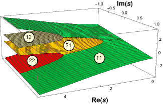
Figure 1: Illustration for the sheet labeling in the case of two channels.

Table 2: The notation of the Riemann sheets with the sign of the imaginary part of the c.m. momentum of each channel.

Riemann sheet	Sign of imaginary part of channel momentum
RS111	$\operatorname{Im}(p_{1})~{}>~{}0$	$\operatorname{Im}(p_{2})~{}>~{}0$	$\operatorname{Im}(p_{3})~{}>~{}0$
RS211	$\operatorname{Im}(p_{1})~{}<~{}0$	$\operatorname{Im}(p_{2})~{}>~{}0$	$\operatorname{Im}(p_{3})~{}>~{}0$
RS221	$\operatorname{Im}(p_{1})~{}<~{}0$	$\operatorname{Im}(p_{2})~{}<~{}0$	$\operatorname{Im}(p_{3})~{}>~{}0$
RS222	$\operatorname{Im}(p_{1})~{}<~{}0$	$\operatorname{Im}(p_{2})~{}<~{}0$	$\operatorname{Im}(p_{3})~{}<~{}0$
RS121	$\operatorname{Im}(p_{1})~{}>~{}0$	$\operatorname{Im}(p_{2})~{}<~{}0$	$\operatorname{Im}(p_{3})~{}>~{}0$
RS112	$\operatorname{Im}(p_{1})~{}>~{}0$	$\operatorname{Im}(p_{2})~{}>~{}0$	$\operatorname{Im}(p_{3})~{}<~{}0$
RS212	$\operatorname{Im}(p_{1})~{}<~{}0$	$\operatorname{Im}(p_{2})~{}>~{}0$	$\operatorname{Im}(p_{3})~{}<~{}0$
RS122	$\operatorname{Im}(p_{1})~{}>~{}0$	$\operatorname{Im}(p_{2})~{}<~{}0$	$\operatorname{Im}(p_{3})~{}<~{}0$

The poles correspond to bound states or resonances depending on their location on the Riemann sheets. Bound states correspond to poles on the physical sheet below the lowest threshold energy and resonances are poles in the complex plane of the unphysical sheets (in addition there are virtual state poles, located on the real axis of unphysical sheets, but those do not play a role in this work). The poles on the sheets closest to the physical sheet have the strongest influence on the scattering amplitude. In the current notation sheets RS211, RS221, and RS222 would be directly connected to the physical sheet, i.e., RS111, above the respective thresholds (c.f. Fig. 1). The poles of the $T$-matrix are given by the zeroes of the determinant of the matrix in Eq. (4), i.e.,

$${\rm det}\left(K^{-1}(s)+(I_{\rm CM}(s)-I_{\rm CM}(m^{2}))\right)=0.$$ (8)

The unphysical sheets can be accessed by adding the discontinuity across the branch cut to Eq. (4). Via the Schwarz reflection principle the discontinuity across the branch cut is related to the imaginary part of the amplitude by

$$\operatorname{Disc}\left[T_{K}(s)\right]=T_{K}(s{+}i\epsilon)-T_{K}(s-i\epsilon)=2i\,\operatorname{Im}[T_{K}(s{+}i\epsilon)],$$ (9)

where $\operatorname{Im}[T_{K}(s{+}i\epsilon)]$ needs to be understood as the analytic continuation of the imaginary part of the amplitude on the real axis above threshold.

Crossing from the physical sheet (RS111) to any sheet can be done by

$$T_{K,X}^{-1}(s)=T_{K}^{-1}(s)+\operatorname{Disc}_{X}[T_{K}^{-1}(s)],$$ (10)

where the subscript $X$ stands for the sheet number and $\operatorname{Disc}$ is a $3\times 3$ matrix containing the relevant discontinuities needed for the sheet transition, e.g. for the transition from RS111 to RS211 we employ

$$\operatorname{Disc}_{211}T_{K}^{-1}=2i\left[\hskip-5.0pt\begin{array}[]{r*\c@MaxMatrixCols{M{2em}}}-\rho_{1}&0.00003pt{\hss$0$}&0.00003pt{\hss$0$}\\ 0&0.00003pt{\hss$0$}&0.00003pt{\hss$0$}\\ 0&0.00003pt{\hss$0$}&0.00003pt{\hss$0$}\end{array}\hskip-5.0pt\right],$$ (11)

and for RS111 to RS221

$$\operatorname{Disc}_{221}T_{K}^{-1}=2i\left[\hskip-5.0pt\begin{array}[]{r*\c@MaxMatrixCols{M{2em}}}-\rho_{1}&0.00003pt{\hss$0$}&0.00003pt{\hss$0$}\\ 0&0.00003pt{\hss$-\rho_{2}$}&0.00003pt{\hss$0$}\\ 0&0.00003pt{\hss$0$}&0.00003pt{\hss$0$}\end{array}\hskip-5.0pt\right].$$ (12)

This prescription is straightforwardly generalized to arbitrary transitions between sheets.

At a pion mass of about 391 MeV, the lowest pole in the studied channel turns out to be a bound state, accordingly located on sheet RS111 Moir et al. [2016]; the same conclusion was reached in UChPT in Ref. Albaladejo et al. [2017]. This pole was found in the fits of all 9 parametrizations employed by the Hadron Spectrum Collaboration Moir et al. [2016]. At the same time, additional poles were found on sheets RS211, RS221, and RS222. These additional poles were found for almost all amplitude paramterizations employed in Ref. Moir et al. [2016], which were, however, not reported in the publication since they not only scatter very much, but also are in parts located outside the energy region where the fit was performed. Table 3 shows the pole values found from the search with the corresponding sheets from the different amplitude parametrizations. The $1\sigma$ uncertainties of the pole values were calculated by the bootstrap method.

Table 3: The pole locations from amplitude parametrizations of Ref. Moir et al. [2016], in units of MeV. Empty slots denote that a pole was not found within the search range for the particular parametrization on the corresponding sheet. In the last line the results for the UChPT amplitude employed in Ref. Albaladejo et al. [2017] are given for comparison.

Amplitudes	RS111	RS211	RS221	RS222
Amplitude 1	$2275.92$	$2720_{-89}^{+150}\,-i\,198_{-70}^{+37}$	$3060_{-120}^{+210}\,-i\,133_{-45}^{+100}$	$3030_{-130}^{+260}\,-i\,430_{-120}^{+210}$
Amplitude 2	$2275.92$	$2717_{-51}^{+99}\,-i\,204_{-47}^{+45}$	$3070_{-110}^{+190}\,-i\,141_{-55}^{+120}$	$3080_{-120}^{+230}\,-i\,420_{-120}^{+200}$
Amplitude 3	$2275.92$		$3710_{-180}^{+210}\,-i\,706_{-87}^{+150}$	$3880_{-200}^{+210}\,-i\,1153_{-79}^{+110}$
Amplitude 4	$2275.94$		$3710_{-170}^{+230}\,-i\,461_{-64}^{+150}$	$3840_{-180}^{+260}\,-i\,763_{-58}^{+130}$
Amplitude 5	$2276.04$	$2789_{-54}^{+590}\,-i\,27_{-27}^{+210}$	$3560_{-110}^{+130}\,-i\,311_{-42}^{+98}$	$3680_{-120}^{+140}\,-i\,601_{-40}^{+91}$
Amplitude 6	$2275.70$	$2618_{-50}^{+64}\,-i\,240_{-35}^{+56}$	$3075_{-67}^{+85}\,-i\,240_{-38}^{+51}$	$3162_{-82}^{+100}\,-i\,349_{-45}^{+64}$
Amplitude 7	$2275.98$	$2652_{-53}^{+70}\,-i\,291_{-41}^{+57}$	$3096_{-80}^{+100}\,-i\,300_{-36}^{+51}$	$3180_{-91}^{+120}\,-i\,410_{-55}^{+70}$
Amplitude 8	$2275.70$	$2621_{-67}^{+90}\,-i\,242_{-31}^{+34}$	$3064_{-59}^{+66}\,-i\,251_{-55}^{+45}$	$3141_{-74}^{+80}\,-i\,318_{-48}^{+96}$
Amplitude 9	$2275.92$	$2673_{-25}^{+28}\,-i\,182_{-26}^{+23}$	$2866_{-40}^{+38}\,-i\,154_{-11}^{+13}$	$2909_{-38}^{+38}\,-i\,274_{-22}^{+26}$
UChPT	$2263^{+8}_{-14}$	$2633_{-43}^{+79}\,-i\,114_{-12}^{+11}$	$2467_{-25}^{+32}\,-i\,113_{-16}^{+18}$	$3000_{-110}^{+290}\,-i\,93_{-15}^{+21}$

Graphically the poles on RS221 are displayed in Fig. 2. In the following we focus the discussion on this sheet, since this is the one where the UChPT amplitude has its most prominent higher $D_{0}^{*}$ pole at physical Du et al. [2018] as well as the unphysical meson masses employed in the lattice study Albaladejo et al. [2017]. The plots of the pole locations of the higher pole for the different parametrizations on the other Riemann sheets that connect closely to the physical axis (RS211 and RS222) are shown in the Appendix. Table 4 gives the location of the corresponding two particle thresholds.

Table 4: The two particle thresholds in MeV for the pion mass of 391 MeV.

Threshold	Threshold [MeV]
$D\pi$	$2276.49$
$D\eta$	$2472.46$
$D_{s}\bar{K}$	$2500.51$

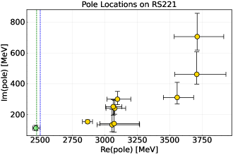
Figure 2: The location of poles on sheet RS221 on the complex energy plane. The $x$-axis and $y$-axis show the real and imaginary part of energy, respectively. The poles from the amplitude parametrizations employed in Ref. Moir et al. [2016] are shown in yellow. The pole from the UChPT amplitude Liu et al. [2013] is shown in green Albaladejo et al. [2017]. The vertical green and blue dashed lines represent the $D\eta$ and $D_{s}\bar{K}$ thresholds, respectively. The error bars show the $1\sigma$ statistical uncertainty.

Figure 2 and Fig. 13 in the Appendix and Table 3 clearly show two important features of the poles extracted from different parametrizations: $(i)$ There is a significant correlation between real part and imaginary part of the poles, and the location of the pole extracted from the UChPT analysis is in line with that correlation. $(ii)$ All poles are located on hidden sheets, which are the sheets that are not directly connected to the physical sheet. For example, the RS221 poles are well above the $D_{s}\bar{K}$ threshold. Thus they are all shielded by the RS222 sheet and their effect on the amplitude can hardly be seen above the $D_{s}\bar{K}$ threshold. As we discuss in the following, both features together guide one to an understanding that there indeed needs to be a second pole in an amplitude that describes the lattice data and that it is natural that the original analysis performed on the lattice data lead to badly constrained pole locations. The mechanism underlying this is that the distance from the threshold is overcome by an enhanced residue. This mechanism, also reported e.g. for the case of the $f_{0}(980)$ and $a_{0}(980)$, was observed before as a general feature of Flatté amplitudes Baru et al. [2005].

2.2 Residues and Threshold distance

A resonance is characterized by the pole location, traditionally parametrized as

$$\sqrt{s_{p}}=M-i\Gamma/2.$$ (13)

Please note that the parameters $M$ and $\Gamma$, derived from the pole location, agree to those found e.g. in the BW fits only for narrow, isolated resonances — for details see the review on resonances in Ref. Workman et al. [2022]. Equally fundamental resonance properties are provided by the pole residues. A pole-residue quantifies the couplings of the resonance to the various channels. The residues of a pole located at $s=s_{p}$ are defined as

$$R_{ij}=\lim_{s\to s_{p}}(s-s_{p}){T}_{ij}(s).$$ (14)

The residues can be easily obtained using the L’Hôpital rule to compute the limit:

$$R_{ij}=\left(\frac{d}{ds}{T}_{ij}^{-1}\right)^{-1}_{s=s_{p}}.$$ (15)

Since the residues factorize according to $R_{ij}^{2}=R_{ii}R_{jj}$ one can define an effective coupling via

$$g^{r}_{i}=R_{ij}/\sqrt{R_{jj}},$$ (16)

which has dimension [mass]. The index $r$ is meant to distinguish the residues from the parameters $g_{i}$ that appear in the $K$-matrix in Eq. (2). The couplings $g^{r}_{i}$ characterize the transition strengths of the resonance to the channel. Those residues can also be extracted from production reactions and are independent of how the resonance was produced.

Since the poles of interest here are hidden, their effect on the physical axis is visible only at the thresholds irrespective of their exact pole locations. Moreover, the visible effect in the amplitude on the physical axis from a pole on a hidden sheet close to the threshold with a small residue is in fact hardly distinguishable from a faraway pole with a large residue. We regard this ambiguity as the most natural explanation for the large spread in the pole locations found in the analysis of the lattice data reported above.

To test this hypothesis, we now study the strengths of the residues as functions of the distance of the poles to the threshold. Clearly, there is some ambiguity in how to quantify the distance from the threshold. Since the channel couplings also drive the size of the imaginary part of the pole location and we want to avoid counting the effect of those couplings twice, we choose instead of $\sqrt{(M-M_{\rm thr.})^{2}+(\Gamma/2)^{2}}$, which might appear more natural on the first glance,

$${\rm Dist}=M-M_{\rm thr.}$$ (17)

as a measure for the distance of the pole to the threshold. The pole mass $M$ that appears above was introduced in Eq. (13) and $M_{\rm thr.}$ denotes the threshold location relevant for the given sheet, e.g. in case of RS221 we have $M_{\rm thr.}=M_{K}+M_{D_{s}}$.

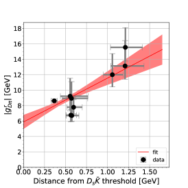
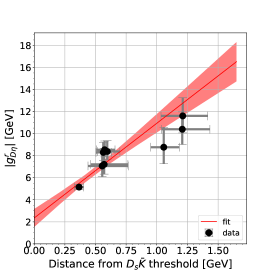
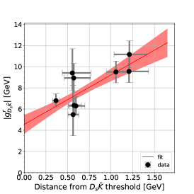
Figure 3: The distance of the real part of the pole on sheet RS221 from the $D_{s}\bar{K}$ threshold versus the effective coupling of the pole to the $D\pi$ channel (left), $D\eta$ channel (middle) and $D_{s}\bar{K}$ channel (right). The red line shows the straight line fit. The red band encloses the $1\sigma$ uncertainty of the fit.

Table 5 shows the distance of the RS221 pole from the $D_{s}\bar{K}$ threshold along with the square root of the absolute value of the residue to the three channels. The graphical representation for the $D\pi\text{-}D\pi$ channel is shown in Fig. 3 (left). A straight line is fit to the data to extrapolate the values at the threshold. The fitting was done using the MINUIT algorithm James and Roos [1975] from the iminuit interface  Dembinski et al. [2022], Guo . The uncertainties of the fit parameters quoted are from the MIGRAD routine of MINUIT. The $1\sigma$ statistical uncertainty of the fitted line was calculated using the bootstrap technique. From the straight line fit the $y$-intercept was found to be at $(5.8\pm{0.9})$ GeV. The graphical representation for corresponding distances and residues for the $D\eta\text{-}D\eta$ and the $D_{s}\bar{K}\text{-}D_{s}\bar{K}$ channel is given in Fig. 3 (middle) and Fig. 3 (right). The fit to the $D\eta$ ($D_{s}\bar{K}$) residues provides an intercept of $(2.4\pm{0.8})$ GeV  ($(4.6\pm{0.9})$ GeV). The corresponding results for the poles on sheets RS211 and RS222 are shown in the Appendix.

While the linear fits shown do not provide an excellent representation of the extracted data for the different channels, they illustrate nicely that there is indeed a significant correlation between the distance of the poles from the threshold and the residues. In addition, the effect of the poles at threshold, encoded in the $y$ intercepts deduced from the fits, is rather well constrained by the fits. We interpret this observation such that the lattice data require not only one bound state pole but also a higher pole as was also found in the various studies employing UChPT Kolomeitsev and Lutz [2004], Guo et al. [2006, 2007, 2009], Albaladejo et al. [2017], Du et al. [2018], Lutz et al. .

An interesting question is, if it is possible to come up with a parametrization to be used in the $K$-matrix fit that constrains better the pole location of the higher pole, with inputs of approximate symmetries of QCD. This will be the focus of the next section.

Table 5: Distance of the RS221 pole from the $D_{s}\bar{K}$ threshold and the square root of its residue to the respective channels in MeV for the amplitude parametrizations obtained in Ref. Moir et al. [2016]. In the last line the results for the UChPT amplitude employed in Ref. Albaladejo et al. [2017] are given for comparison.

Amplitudes	Dist. from $D_{s}\bar{K}$ thr. [MeV]	$|g_{D\pi}^{r}|$ [GeV]	$|g_{D\eta}^{r}|$ [GeV]	$|g_{D_{s}\bar{K}}^{r}|$ [GeV]
Amplitude 1	$554_{-115}^{+212}$	$9_{-2}^{+2}$	$7_{-1}^{+1}$	$9_{-2}^{+2}$
Amplitude 2	$570_{-110}^{+194}$	$9_{-1}^{+2}$	$7_{-1}^{+2}$	$9_{-1}^{+1}$
Amplitude 3	$1211_{-177}^{+205}$	$16_{-2}^{+3}$	$12_{-2}^{+2}$	$11_{-1}^{+1}$
Amplitude 4	$1208_{-170}^{+226}$	$13_{-2}^{+3}$	$10_{-1}^{+2}$	$10_{-1}^{+1}$
Amplitude 5	$1057_{-107}^{+127}$	$12_{-2}^{+3}$	$9_{-2}^{+2}$	$10_{-1}^{+1}$
Amplitude 6	$596_{-80}^{+103}$	$8_{-1}^{+1}$	$8_{-1}^{+1}$	$6.3_{-0.8}^{+0.9}$
Amplitude 7	$575_{-67}^{+85}$	$7_{-1}^{+1}$	$8.5_{-0.6}^{+0.8}$	$6.3_{-0.8}^{+0.7}$
Amplitude 8	$563_{-59}^{+66}$	$6.8_{-0.9}^{+0.8}$	$8.3_{-0.7}^{+0.9}$	$6_{-2.}^{+3}$
Amplitude 9	$366_{-40}^{+38}$	$8.6_{-0.3}^{+0.3}$	$5.1_{-0.2}^{+0.2}$	$6.8_{-0.6}^{+0.6}$
UChPT	$-34_{-25}^{+32}$	$5.2_{-0.4}^{+0.6}$	$6.7_{-0.4}^{+0.6}$	$13_{-1}^{+2}$

3 SU(3) symmetry

The parametrization dependence of the higher pole location calls for a stronger constrained amplitude. In the following we present a prescription of the $K$-matrix consistent with the SU(3) flavor symmetry. In the resulting scattering matrix SU(3) breaking comes only from the Chew-Mandelstam functions introduced in Eq. (5). Clearly, for the physical pion mass and low energies such a treatment is not justified, since the leading order chiral interaction scales with the energies of pion and kaons for $D\pi$ and $D_{s}\bar{K}$ scattering, respectively, which induces a sizeable SU(3) flavor breaking into the scattering potential. However, in this study we work at higher pion masses which leads to a much smaller pion-kaon mass difference. Moreover, we are mainly interested in the higher mass range, where the second pole is located. Under such circumstances the leading SU(3) breaking effect is induced by the loop functions which bring the cut structure to the amplitudes.

The flavor structure of the $D\Phi$ interaction can be written as a direct product of an anti-triplet for the charmed mesons and an octet for the light pseudoscalar mesons. The direct product can be decomposed into a direct sum of the $[\bar{3}]$, $[6]$ and $[\overline{15}]$ irreducible representations. Figure 4 shows the multiplet structure.

Figure 4: Weight diagrams of the $[\overline{15}],[6]$ and $[\bar{3}]$ representations.

The SU(3) flavor basis and the isospin-symmetric particle basis are related via

$$\begin{pmatrix}\lvert[\bar{3}]\rangle\\ \lvert[6]\rangle\\ \lvert[\overline{15}]\rangle\end{pmatrix}=U\begin{pmatrix}\lvert D\pi\rangle\\ \lvert D\eta\rangle\\ \lvert D_{s}\bar{K}\rangle\end{pmatrix},$$ (18)

where

$$U=\begin{pmatrix}-3/4&-1/4&-\sqrt{3/8}\\ \sqrt{3/8}&-\sqrt{3/8}&-1/2\\ 1/4&3/4&-\sqrt{3/8}\\ \end{pmatrix}.$$ (19)

From the rotation matrix $U$, we may read off the following expressions for the SU(3) symmetric coupling structure of the $D\pi$, $D\eta$ and $D_{s}\bar{K}$ $(I=\frac{1}{2},S=0)$ coupled-channel system:

$$C_{\bar{3}} =\begin{pmatrix}-3/4\\ -1/4\\ -\sqrt{3/8}\end{pmatrix}\begin{pmatrix}-3/4&-1/4&-\sqrt{3/8}\end{pmatrix}$$

$$=\frac{3}{8}\begin{pmatrix}3/2&1/2&\sqrt{3/2}\\ 1/2&1/6&\sqrt{1/6}\\ \sqrt{3/2}&\sqrt{1/6}&1\end{pmatrix}~{},$$ (20)

$$C_{6} =\begin{pmatrix}\sqrt{3/8}\\ -\sqrt{3/8}\\ -1/2\end{pmatrix}\begin{pmatrix}\sqrt{3/8}&-\sqrt{3/8}&-1/2\end{pmatrix}$$

$$=\frac{1}{2}\begin{pmatrix}3/4&-3/4&-\sqrt{3/8}\\ -3/4&3/4&\sqrt{3/8}\\ -\sqrt{3/8}&\sqrt{3/8}&1/2\end{pmatrix}~{},$$ (21)

$$C_{\overline{15}} =\begin{pmatrix}1/4\\ 3/4\\ -\sqrt{3/8}\end{pmatrix}\begin{pmatrix}1/4&3/4&-\sqrt{3/8}\end{pmatrix}$$

$$=\frac{3}{8}\begin{pmatrix}1/6&1/2&-\sqrt{1/6}\\ 1/2&3/2&-\sqrt{3/2}\\ -\sqrt{1/6}&-\sqrt{3/2}&1\end{pmatrix}~{}.$$ (22)

The form of the $K$-matrix assuming the existence of two bare poles, in contrast to the one used in Ref. Moir et al. [2016] which contains only one bare pole, reads

$$K=\left(\frac{g_{\bar{3}}^{2}}{m_{\bar{3}}^{2}-s}{+}c_{\bar{3}}\right)C_{\bar{3}}+\left(\frac{g_{6}^{2}}{m_{6}^{2}-s}{+}c_{6}\right)C_{6}+c_{\overline{15}}\,C_{\overline{15}}.$$ (23)

Here the two bare poles are assumed to be in the two SU(3) multiplets with $S$-wave attractions from the leading order chiral dynamics Albaladejo et al. [2017]. We have seven free parameters in total, $g_{\alpha}$, $c_{\alpha}$ and $m_{\alpha}$. The overall factors in Eq. (22) are absorbed into the parameters of $g_{\alpha}$, $c_{\alpha}$. If there was no SU(3) constraint, a $K$-matrix with the same number of bare poles would contain 3 more parameters (a constant $K$ matrix is symmetric and thus contains 6 parameters, instead of 3 $c_{\alpha}$’s here).

With Eqs. (4) and (5), the $T$-matrix $T_{K}(s)$ can be calculated in the same way as in Sect. 2. The subtraction point for the Chew-Mandelstam function of the fits is chosen identical to the parameter $m_{\bar{3}}$.

4 Fitting to Lattice Energy Levels

Here we employ the flavor SU(3) constrained $K$-matrix to fit the lattice energy levels in the $D\pi$ c.m. frame obtained in Ref. Moir et al. [2016]. To this end, we need to relate the $T$-matrix defined with the $K$-matrix in the continuum system and the energy levels in the finite volume system. In this study, we employ the scheme based on the effective field theory framework developed in Ref. Döring et al. [2011]. Below we briefly summarize this scheme.

With the Lippmann-Schwinger equation, the $T$-matrix in the continuum can be written as

$$T(s)=\frac{1}{V^{-1}(s)-G(s)},$$ (24)

where $V(s)$ is the interaction matrix and $G(s)$ is the diagonal matrix of the scalar two-meson loop functions Oller and Meißner [2001]. With the momentum cut-off regularisation $G(s)$ is given by

$$G_{ii}(s) =\int\displaylimits^{\left|\vec{q}\right|<q_{\rm max}}\frac{d^{3}\vec{q}}{(2\pi)^{3}}\frac{1}{2\omega_{1}^{(i)}(\left|\vec{q}\right|)\omega_{2}^{(i)}(\left|\vec{q}\right|)}$$

$$\hskip 28.45274pt\times\frac{\omega_{1}^{(i)}(\left|\vec{q}\right|)+\omega_{2}^{(i)}(\left|\vec{q}\right|)}{s-(\omega_{1}^{(i)}(\left|\vec{q}\right|)+\omega_{2}^{(i)}(\left|\vec{q}\right|)^{2}},$$ (25)

$$\omega^{(i)}_{1,2}(\vec{q}) =\sqrt{m^{2(i)}_{1,2}+\vec{q}^{2}},$$ (26)

where $q_{\rm max}$ is the cut-off momentum and $m^{(i)}_{1,2}$ are the masses of the two particles in channel $i$. Similarly to Eq. (24), the $T$-matrix in a finite volume system $\tilde{T}$ satisfies

$$\tilde{T}(s)=\frac{1}{\tilde{V}^{-1}(s)-\tilde{G}(s)},$$ (27)

where $\tilde{V}(s)$ and $\tilde{G}(s)$ are the interaction and loop function in the finite volume system, respectively. With the spatial extension $L$ of the cubic box, $\tilde{G}(s)$ is given as

$$\tilde{G}_{ii}(s)= \,\frac{1}{L^{3}}\sum_{\vec{q}}^{\left|\vec{q}\right|<q_{\rm max}}\frac{1}{2\omega_{1}^{(i)}(|\vec{q}|)\omega_{2}^{(i)}(|\vec{q}|)}$$

$$\times\frac{\omega_{1}^{(i)}(|\vec{q}|)+\omega_{2}^{(i)}(|\vec{q}|)}{s-(\omega_{1}^{(i)}(|\vec{q}|)+\omega_{2}^{(i)}(|\vec{q}|))^{2}},$$ (28)

with

$$\vec{q}=\frac{2\pi}{L}\vec{n},\,\vec{n}\in\mathbb{Z}^{3}.$$ (29)

Since $V(s)$ is equal to $\tilde{V}(s)$ up to exponentially suppressed corrections, the $T$-matrix in the finite volume system $\tilde{T}$ is related to the $T$-matrix in the infinite volume $T$  by

$$\tilde{T}(s) =\frac{1}{T^{-1}(s)-\Delta G(s)},$$ (30)

with

$$\Delta G_{ii} =\tilde{G}_{ii}(s)-G_{ii}(s).$$ (31)

The lattice energy levels, which we need to fit, correspond to the zeroes of the determinant of $\tilde{T}^{-1}$ provided in Eq. (30).

4.1 Results for the fits employing SU(3) constraints

We performed four different fits to the rest frame lattice energy levels in Ref. Moir et al. [2016] using the MINUIT algorithm James and Roos [1975] with the Julia interface to the iminuit package Dembinski et al. [2022], Guo :

• in Fit 1_4L all the parameters in Eq. (23) are included;

• in Fit 2_4L we fix $c_{\bar{3}}=0$ and $c_{6}=0$;

• in Fit 3_4L we fix $c_{6}=0$;

• in Fit 4_4L we fix $g_{6}=0$ to omit the explicit pole term of $[6]$ (and thus $m_{6}$ is absent).

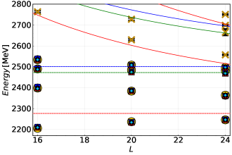
Figure 5: Comparison of the energy levels from data and the fits. The energy levels from Ref. Moir et al. [2016] are shown in yellow. The energy levels used as input in the fits are shown as circles and those not used is shown as crosses. The energy levels from Fit 1_4L, Fit 2_4L, Fit 3_4L and Fit 4_4L are shown in red, blue, black and light blue, respectively. The solid(dashed) red, green and blue lines show the $D\pi$, $D\eta$ and $D_{s}\bar{K}$ non-interacting energy levels(thresholds) respectively.

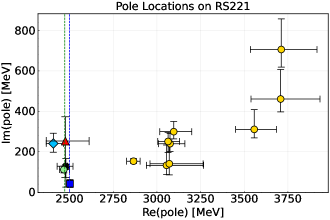
Figure 6: Locations of the RS221 poles from the different fits based on Eq. (23), together with the pole reported in UChPT amplitude Albaladejo et al. [2017] in green, and the various extractions from the amplitudes extracted in Ref. Moir et al. [2016] in yellow. The pole locations from Fit 1_4L, Fit 2_4L, Fit 3_4L and Fit 4_4L are shown in red, blue, black and light blue respectively. The green and blue vertical dashed lines represent the $D\eta$ and $D_{s}\bar{K}$ thresholds, respectively.

From every volume we use the lowest four energy levels (thus the addition _4L to the fit names) of the [000] $A^{+}_{1}$ irreducible representation, where the $S$-wave component gives the dominant contribution. In the next subsection we discuss the fit results for Fit 4_All that was performed including all the rest frame lattice levels. The obtained parameters for the different fits as well as the $\chi^{2}$ values found are listed in Table 6. Figure 5 shows the energy levels obtained from the fits together with the data points in the lattice rest frame. The uncertainties of the fit parameters quoted are from the MIGRAD routine of MINUIT. Further, using the parameters from the fit, the poles of the $T$-matrix in the continuum on the different Riemann sheets are extracted. The resulting pole positions can be found in Table 7. It turns out that, contrary to the pole extraction employing Eq. (2), now in all fits the higher mass pole has a mass of about 2.5 GeV and is thus located close the $D\eta$ and $D_{s}\bar{K}$ thresholds (see Fig. 6)

A more detailed comparison of the performance of the fits shows that for $[\bar{3}]$ both a pole term and a constant term are needed to obtain an acceptable fit. Moreover, the uncertainties for the pole parameters that emerged from Fit 1_4L are a lot larger than for the other fits (in addition the fit even allows for an additional level very close to the fitting range). We therefore exclude both Fit 1_4L and Fit 2_4L from further discussions. On the other hand, fits of comparable quality emerge, if either the constant term in the $[6]$ (Fit 3_4L) or the pole term in the $[6]$ (Fit 4_4L) is abandoned. In the latter case the higher pole is generated via the unitarization. Note that in our case the number of parameters connected to the bound state pole is in any case 2 (one coupling constant and a mass), while in case of the fits performed by the Hadron Spectrum Collaboration this number is 4, for there an individual coupling is needed for each channel. The difference in the number of parameters needed for the $[\bar{3}]$ and the $[6]$ channels can be understood straightforwardly from the observation that the pole in the $[\bar{3}]$ is a bound state and further parameters are needed to obtain a decent fit of the additional energy levels. The pole originated in the $[6]$, on the other hand, sits rather high up in the spectrum, having a larger imaginary part, and thus naturally controls all energy levels that have a sizable contribution from this representation; either the bare pole or the constant term in $[6]$ provides a seed for the $[6]$ pole.

Table 7 also shows that in all fits poles appear on RS222 above the $D_{s}\bar{K}$ threshold, however, with large uncertainties especially on the mass parameters. Since in this energy range RS222 connects directly to the physical sheet, these poles show up as peaks in the amplitudes at high energies. Note that analogous poles were also present in the fits performed in the course of the analysis of Ref. Moir et al. [2016] and in the UChPT amplitude (see Table 3), however, they appeared at significantly higher energies. In Fit 1_4L this pole can appear quite close to the energy region of interest, given the large uncertainty in the mass parameter. We interpret this phenomenon as reflecting a too large number of parameters in the fit. In the two best fits, namely Fit 3_4L and Fit 4_4L, on the other hand, the poles on RS222 are typically located deep inside the complex plane or rather high above the threshold, respectively, although within uncertainties it can appear rather close to threshold also for Fit 3_4L, with leads to the strong rise very close to the higher thresholds. The large spread in the amplitudes above the $D_{s}\bar{K}$ threshold visible in Figs. 8 reflects the bad determination of the highest pole from the lattice data included in the fits.

A comparison of the RS111 pole locations from the SU(3) fits just reported and that the UChPT amplitude Albaladejo et al. [2017] and Ref. Moir et al. [2016] is shown in Fig. 7. As expected the location of this bound state pole is consistent amongst all extractions.

Note that in all fits the constant term in the $[\overline{15}]$ representation turns out to be repulsive, in line with the expectations from leading order chiral perturbation theory. This is a nice and in fact non-trivial confirmation of the hypothesis that, even at pion masses as high as 391 MeV, already leading order chiral perturbation theory provides valuable guidance for the physics that leads to the emergence or not appearance of hadronic molecules.

We also tested if we can fit the lattice data when replacing the pole term in the $[6]$ representation by a pole in the $[\overline{15}]$. Those fits, however, did not converge and are therefore not reported in the figures and tables. The amplitudes arrived from the fits are shown in Fig. 8, there, however, at significantly higher energies. The appearance of these poles in a direct consequence of the $K$-matrix parametrization employed. Moreover, in Fit 1_4L and Fit 2_4L those poles are rather close to the threshold

Table 6: The best fit values arrived in the different fits to the lattice energy levels of Ref. Moir et al. [2016] based on Eq. (23), along with their $\chi^{2}/\mbox{dof}$. The symbol ’-’ is used for parameters set to zero (or absent) in the particular fit.

	$g_{3}$ [GeV]	$m_{\bar{3}}$ [MeV]	$g_{6}$ [GeV]	$m_{6}$ [MeV]	$c_{\bar{3}}$	$c_{6}$	$c_{\overline{15}}$	$\chi^{2}$	$\chi^{2}/\mbox{dof}$
Fit 1_4L	$2.92\pm 0.39$	$2275.1\pm 0.6$	$0.32\pm 0.32$	$2542\pm 50$	$4\pm 3$	$0.7\pm 0.4$	$-0.6\pm 0.2$	7.1	$1.4$
Fit 2_4L	$2.31\pm 0.14$	$2274.5\pm 0.8$	$0.66\pm 0.17$	$2560\pm 37$	-	-	$-0.6\pm 0.2$	14	$1.9$
Fit 3_4L	$2.91\pm 0.39$	$2275.1\pm 0.6$	$1.20\pm 0.62$	$2735\pm 266$	$4\pm 2$	-	$-0.6\pm 0.2$	7.3	$1.2$
Fit 4_4L	$3.16\pm 0.38$	$2275.3\pm 0.6$	-	-	$5\pm 2$	$1.0\pm 0.2$	$-0.4\pm 0.2$	8.2	$1.2$
Fit 4_All	$2.4\pm 0.2$	$2274.8\pm 0.6$	-	-	$1.1\pm 0.4$	$0.54\pm 0.06$	$-0.26\pm 0.09$	$29.6$	$2.1$

Table 7: The pole locations from the different fits.

Fits	RS111	RS211	RS221	RS222
Fit 1_4L	$2275.1^{+0.6}_{-0.6}-0\mathit{i}$	$2515^{+88}_{-19}-23^{+19}_{-88}\mathit{i}$	$2476^{+136}_{-109}-253^{+181}_{-120}\mathit{i}$	$2544^{+151}_{-46}-18^{+18}_{-69}\mathit{i}$
Fit 2_4L	$2274.5^{+0.8}_{-0.7}-0\mathit{i}$	$2498^{+9}_{-10}-20^{+7}_{-6}\mathit{i}$	$2503^{+12}_{-13}-42^{+19}_{-22}\mathit{i}$	$2518^{+19}_{-21}-63^{+31}_{-44}\mathit{i}$
Fit 3_3L	$2275.1^{+0.6}_{-0.6}-0\mathit{i}$	$2512^{+22}_{-67}-50^{+37}_{-20}\mathit{i}$	$2479^{+41}_{-50}-128^{+103}_{-38}\mathit{i}$	$2571^{+250}_{-135}-314^{+265}_{-84}\mathit{i}$
Fit 4_4L	$2275.3^{+0.6}_{-0.6}-0\mathit{i}$	$2518^{+28}_{-17}-92^{+18}_{-28}\mathit{i}$	$2407^{+59}_{-40}-241^{+43}_{-50}\mathit{i}$	$2673^{+94}_{-44}-61^{+19}_{-47}\mathit{i}$
Fit 4_All	$2274.8^{+0.6}_{-0.6}-0\mathit{i}$	$2681^{+46}_{-33}-263^{+43}_{-51}\mathit{i}$	$2516^{+71}_{-60}-479^{+38}_{-50}\mathit{i}$	$3123^{+144}_{-99}-359^{+86}_{-162}\mathit{i}$

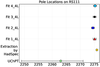
Figure 7: Locations of the RS111 poles from the different fits together with the RS111 pole in the UChPT amplitude Albaladejo et al. [2017] and from HadSpec Moir et al. [2016].

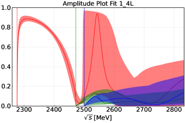
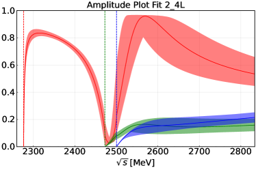
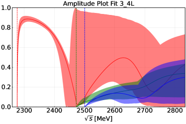
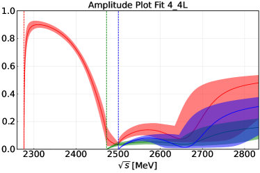
Figure 8: The resulting amplitudes from the various fits in the form of $\rho^{2}|T|^{2}$. The $D\pi\text{-}D\pi,D\eta\text{-}D\eta$ and $D_{s}\bar{K}\text{-}D_{s}\bar{K}$ amplitudes are shown in red, green and blue, respectively. The vertical red, green and blue dashed lines show the $D\pi$, $D\eta$ and the $D_{s}\bar{K}$ thresholds, respectively. The error bands cover the 1$\sigma$ statistical uncertainties.

To complete the discussion, in Table 8 we show the square root of the absolute values of the RS221 pole residues to the respective channels derived from the fits. Further, Fig. 9 shows the distance of the RS221 pole to the $D_{s}\bar{K}$ threshold, as defined in Eq. (17), versus the effective coupling of the pole to the $D\pi$, $D\eta$ and $D_{s}\bar{K}$ channels, respectively. Besides Fit 4_4L, all values are statistically consistent with the intercepts arrived at in Section 2.2 within errors.

Table 8: The absolute value of the square root of the RS221 pole residues obtained by the SU(3) flavor constrained $K$-matrix to the respective channels.

Parameter set	$|g_{D\pi}^{r}|$ [GeV]	$|g_{D\eta}^{r}|$ [GeV]	$|g_{D_{s}\bar{K}}^{r}|$ [GeV]
Fit 1_4L	$12_{-2}^{+7}$	$8_{-2}^{+2}$	$17_{-10}^{+2}$
Fit 2_4L	$5_{-1}^{+1}$	$4_{-1}^{+1}$	$5_{-2}^{+2}$
Fit 3_4L	$10_{-5}^{+1}$	$6_{-3}^{+1}$	$10_{-5}^{+3}$
Fit 4_4L	$11_{-2}^{+2}$	$9_{-2}^{+3}$	$19_{-2}^{+3}$
Fit 4_All	$13.4_{-0.5}^{+0.5}$	$8.5_{-0.7}^{+0.8}$	$17.8_{-0.9}^{+0.8}$

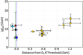
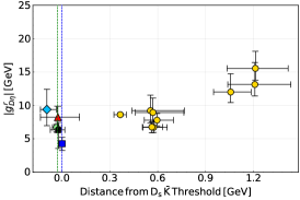
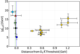
Figure 9: The distance of the real part of the pole on RS221 from the $D_{s}\bar{K}$ threshold versus the effective coupling of the pole to the $D\pi$ channel (left), $D\eta$ channel (centre) and $D_{s}\bar{K}$ channel (right). The data points from Fit 1_4L, Fit 2_4L, Fit 3_4L and Fit 4_4L are shown in red, blue, black and light blue, respectively. Those for the amplitudes obtained in Ref. Moir et al. [2016] are shown in yellow and UChPT amplitude Albaladejo et al. [2017] in green. The green and blue vertical dashed lines show the $D\eta$ and $D_{s}\bar{K}$ thresholds, respectively. The error bars represent the 1$\sigma$ statistical uncertainty.

4.2 Inclusion of the Higher Lattice Levels

Our fit amplitudes are formulated as a momentum expansion. Accordingly, to find our main results, we performed fits with including only the lowest 4 lattice levels at each volume. However, to check for stability of our findings, we also performed fits with Fit 3 and Fit 4 to all rest frame levels ([000] $A^{+}_{1}$ irrep.) — the resulting fits are labeled as Fit 3_ALL and Fit 4_All. It turns out that the former parametrization does not allow for a decent fit (the best $\chi^{2}/$dof we can achieve is 5.5). It calls for introducing additional bare poles or/and momentum-dependent contact terms.

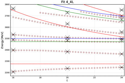
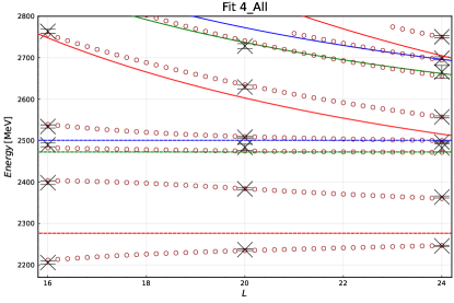
Figure 10: The left panel shows the finite volume energy levels arrived at for Fit 4_4L (only the first four lowest energy levels of each volume included in the fit), while the right panel shows them for Fit 4_All. The black crosses are the lattice energy level data. The dark red circles show the energy levels from the amplitudes. The solid lines show the non-interacting energy levels while the dashed line shows the thresholds. The $D\pi$, $D\eta$ and $D_{s}\bar{K}$ energies are shown in red, green and blue, respectively.

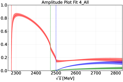
Figure 11: The resulting amplitudes of Fig 4_ALL in the form of $\rho^{2}|T|^{2}$. The $D\pi\text{-}D\pi,D\eta\text{-}D\eta$ and $D_{s}\bar{K}\text{-}D_{s}\bar{K}$ amplitudes are shown in red, green and blue respectively. The vertical red, green and blue lines show the $D\pi$, $D\eta$ and the $D_{s}\bar{K}$ thresholds, respectively. The error bands cover the 1$\sigma$ statistical uncertainties.

In the left panel of Fig.10 we show a comparison of the original fit, Fit 4_4L, with the full spectrum, in the right panel the fit results for Fit 4_All, where the higher levels are included in the fit. The parameters arrived from the new fit are also shown in Table 6. Clearly, the fit is not excellent, however, when compared to only the rest frame levels, amplitude 4 and amplitude 6 from Ref. Moir et al. [2016] reach $\chi^{2}$ values of $36$ and $24$, respectively, and are thus of similar quality. The amplitude plots arrived from Fit 4_All are shown in Fig. 11. Though the bound state pole does not change, there is a change in the location of the higher pole in sheet RS221, which however has a real part similar to that from Fit 4_4L. The previous pole location (from Fit 4_4L) and the new pole location found from fitting including the higher energy levels are shown in Fig.12. We therefore conclude that it is a stable result from our analysis that, as soon as SU(3) constraints are included in the fits, there are always poles close to the $D_{s}\bar{K}$ and $D\eta$ threshold — we do not find anymore the large scatter of the original amplitudes.

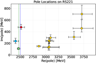
Figure 12: Comparison of locations of the RS221 poles. The pole for Fit 4_All is shown in red, together with the pole reported in UChPT amplitude Albaladejo et al. [2017] in green, and the various extractions from the amplitudes extracted in Ref. Moir et al. [2016] in yellow. The pole location from Fit 4_4L, when including only the lower energy levels, is shown in light blue. The green and blue vertical dashed lines represent the $D\eta$ and $D_{s}\bar{K}$ thresholds, respectively.

5 Summary and Discussion

We investigated the pole content of the nine $K$-matrix parametrizations provided in Ref. Moir et al. [2016] in an analysis of lattice data for open charm states in the $(S=0,I=\frac{1}{2})$ channel. In addition to the bound state pole reported in Ref. Moir et al. [2016], in every amplitude additional poles were found on unphysical Riemann sheets, however, their locations vary strongly between the different parametrizations. On the other hand various investigations employing UChPT find that the structure observed in various experiments in the channel $(S=0,I=\frac{1}{2})$ with open charm originates from the interplay of two $D_{0}^{*}$ poles. In this paper we explain the origin of this seeming contradiction. In particular it is shown that also in the lattice analysis two poles are needed and that, although the poles scatter so dramatically in location, their effects on the amplitudes were comparable in all parametrizations. This is possible since all poles are located on an hidden sheet, such that their effect on the scattering amplitude becomes visible at the threshold. In such a situation the distance from the threshold can be overcome by an enhanced residue. This mechanism was observed before as a general feature of Flatté amplitudes Baru et al. [2005].

To discuss the location of the higher pole directly from the lattice data, we propose to use an amplitude constrained by SU(3) flavor symmetry. The flavor constrained amplitude well reproduces the energy levels and produces a pole in the RS221 sheet close to $D\eta$ and $D_{s}\bar{K}$ thresholds consistent to that of the UChPT amplitude. Such an SU(3) symmetric construction of the $K$ matrix may be used in analyzing other lattice data and also experimental data where multiple channels are involved.

Appendix A Additional information

In this appendix we provide additional Figs.13-15 completing the presentation. In particular we show the analogous pole analysis for RS221 presented in the main text for poles on other sheets.

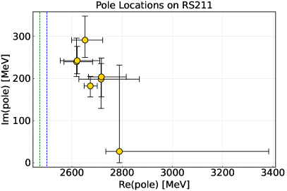
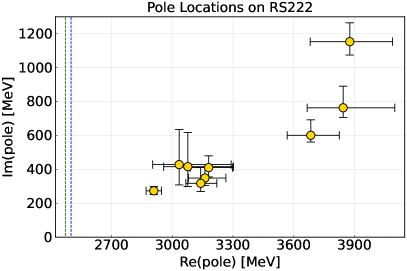
Figure 13: Pole locations on sheet RS211 (left) and on sheet RS222 (right) of the complex energy plane. The vertical green and blue dashed lines represent the $D\eta$ and $D_{s}\bar{K}$ thresholds, respectively. The error bars show the $1\sigma$ statistical uncertainty.

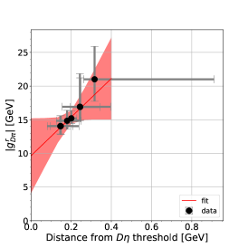
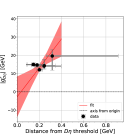
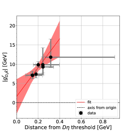
Figure 14: The distance of real part of the pole on sheet RS211 from $D\eta$ threshold versus the effective coupling of the pole to the $D\pi$ channel (left), $D\eta$ channel (center) and $D_{s}\bar{K}$ channel (right). The red line shows the straight line fit. The red band encloses the 1$\sigma$ uncertainty of the fit.

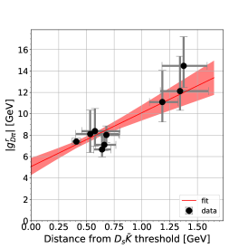
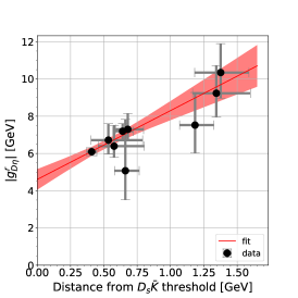
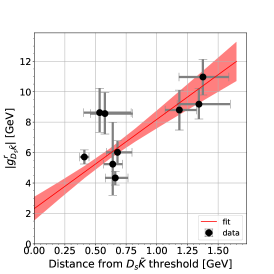
Figure 15: The distance of real part of the pole on sheet RS222 from $D_{s}\bar{K}$ threshold versus the effective coupling of the pole to the $D\pi$ channel (left), $D\eta$ channel (center) and $D_{s}\bar{K}$ channel (right). The red line shows the straight line fit. The red band encloses the 1$\sigma$ uncertainty of the fit.

References

- Aubert et al. [2003] B. Aubert et al. Observation of a narrow meson decaying to at a mass of 2.32-GeV/. Phys. Rev. Lett., 90:242001, 2003. doi:10.1103/PhysRevLett.90.242001.
- Besson et al. [2003] D. Besson et al. Observation of a narrow resonance of mass 2.46-GeV/ decaying to and confirmation of the state. Phys. Rev. D, 68:032002, 2003. doi:10.1103/PhysRevD.68.032002. [Erratum: Phys.Rev.D 75, 119908 (2007)].
- Godfrey and Isgur [1985] S. Godfrey and Nathan Isgur. Mesons in a Relativized Quark Model with Chromodynamics. Phys. Rev. D, 32:189–231, 1985. doi:10.1103/PhysRevD.32.189.
- Abe et al. [2004] Kazuo Abe et al. Study of decays. Phys. Rev. D, 69:112002, 2004. doi:10.1103/PhysRevD.69.112002.
- Aubert et al. [2009] Bernard Aubert et al. Dalitz Plot Analysis of . Phys. Rev. D, 79:112004, 2009. doi:10.1103/PhysRevD.79.112004.
- Aaij et al. [2015a] Roel Aaij et al. Dalitz plot analysis of decays. Phys. Rev. D, 92(3):032002, 2015a. doi:10.1103/PhysRevD.92.032002.
- Aaij et al. [2015b] Roel Aaij et al. Amplitude analysis of decays. Phys. Rev. D, 92(1):012012, 2015b. doi:10.1103/PhysRevD.92.012012.
- Workman et al. [2022] R. L. Workman et al. Review of Particle Physics. PTEP, 2022:083C01, 2022. doi:10.1093/ptep/ptac097.
- Du et al. [2019] Meng-Lin Du, Feng-Kun Guo, and Ulf-G. Meißner. Implications of chiral symmetry on -wave pionic resonances and the scalar charmed mesons. Phys. Rev. D, 99(11):114002, 2019. doi:10.1103/PhysRevD.99.114002.
- Kolomeitsev and Lutz [2004] E. E. Kolomeitsev and M. F. M. Lutz. On Heavy light meson resonances and chiral symmetry. Phys. Lett. B, 582:39–48, 2004. doi:10.1016/j.physletb.2003.10.118.
- Guo et al. [2006] Feng-Kun Guo, Peng-Nian Shen, Huan-Ching Chiang, Rong-Gang Ping, and Bing-Song Zou. Dynamically generated heavy mesons in a heavy chiral unitary approach. Phys. Lett. B, 641:278–285, 2006. doi:10.1016/j.physletb.2006.08.064.
- Guo et al. [2007] Feng-Kun Guo, Peng-Nian Shen, and Huan-Ching Chiang. Dynamically generated heavy mesons. Phys. Lett. B, 647:133–139, 2007. doi:10.1016/j.physletb.2007.01.050.
- Guo et al. [2009] Feng-Kun Guo, Christoph Hanhart, and Ulf-G. Meißner. Interactions between heavy mesons and Goldstone bosons from chiral dynamics. Eur. Phys. J. A, 40:171–179, 2009. doi:10.1140/epja/i2009-10762-1.
- Albaladejo et al. [2017] Miguel Albaladejo, Pedro Fernandez-Soler, Feng-Kun Guo, and Juan Nieves. Two-pole structure of the . Phys. Lett. B, 767:465–469, 2017. doi:10.1016/j.physletb.2017.02.036.
- Du et al. [2018] Meng-Lin Du, Miguel Albaladejo, Pedro Fernández-Soler, Feng-Kun Guo, Christoph Hanhart, Ulf-G. Meißner, Juan Nieves, and De-Liang Yao. Towards a new paradigm for heavy-light meson spectroscopy. Phys. Rev. D, 98(9):094018, 2018. doi:10.1103/PhysRevD.98.094018.
- Guo et al. [2019] Xiao-Yu Guo, Yonggoo Heo, and Matthias F.M. Lutz. On chiral extrapolations of coupled-channel reaction dynamics for charmed mesons. PoS, LATTICE2018:085, 2019. doi:10.22323/1.334.0085.
- [17] Matthias F. M. Lutz, Xiao-Yu Guo, Yonggoo Heo, and C. L. Korpa. Coupled-channel dynamics with chiral long-range forces in the open-charm sector of QCD. arXiv:2209.10601 [hep-ph].
- [18] Csaba L. Korpa, Matthias F. M. Lutz, Xiao-Yu Guo, and Yonggoo Heo. A coupled-channel system with anomalous thresholds and unitarity. arXiv:2211.03508 [hep-ph].
- Liu et al. [2013] Liuming Liu, Kostas Orginos, Feng-Kun Guo, Christoph Hanhart, and Ulf-G. Meißner. Interactions of charmed mesons with light pseudoscalar mesons from lattice QCD and implications on the nature of the . Phys. Rev. D, 87(1):014508, 2013. doi:10.1103/PhysRevD.87.014508.
- Aaij et al. [2016] Roel Aaij et al. Amplitude analysis of decays. Phys. Rev. D, 94(7):072001, 2016. doi:10.1103/PhysRevD.94.072001.
- Aaij et al. [2014] Roel Aaij et al. Dalitz plot analysis of decays. Phys. Rev. D, 90(7):072003, 2014. doi:10.1103/PhysRevD.90.072003.
- Aaij et al. [2015c] R. Aaij et al. First observation and amplitude analysis of the decay. Phys. Rev. D, 91(9):092002, 2015c. doi:10.1103/PhysRevD.91.092002. [Erratum: Phys.Rev.D 93, 119901 (2016)].
- Meißner [2020] Ulf-G. Meißner. Two-pole structures in QCD: Facts, not fantasy! Symmetry, 12(6):981, 2020. doi:10.3390/sym12060981.
- Moir et al. [2016] Graham Moir, Michael Peardon, Sinéad M. Ryan, Christopher E. Thomas, and David J. Wilson. Coupled-Channel , and Scattering from Lattice QCD. JHEP, 10:011, 2016. doi:10.1007/JHEP10(2016)011.
- Mai et al. [2023] Maxim Mai, Ulf-G. Meißner, and Carsten Urbach. Towards a theory of hadron resonances. Phys. Rept., 1001:1–66, 2023. doi:10.1016/j.physrep.2022.11.005.
- Baru et al. [2005] V. Baru, J. Haidenbauer, C. Hanhart, Alexander Evgenyevich Kudryavtsev, and Ulf-G. Meißner. Flatté-like distributions and the a(0)(980) / f(0)(980) mesons. Eur. Phys. J. A, 23:523–533, 2005. doi:10.1140/epja/i2004-10105-x.
- James and Roos [1975] F. James and M. Roos. Minuit: A System for Function Minimization and Analysis of the Parameter Errors and Correlations. Comput. Phys. Commun., 10:343–367, 1975. doi:10.1016/0010-4655(75)90039-9.
- Dembinski et al. [2022] Hans Dembinski, Piti Ongmongkolkul, Christoph Deil, Henry Schreiner, Matthew Feickert, Andrew, Chris Burr, Jason Watson, Fabian Rost, Alex Pearce, Lukas Geiger, AhmedAbdelmotteleb, Bernhard M. Wiedemann, Christoph Gohlke, Gonzalo, Jeremy Sanders, Jonas Drotleff, Jonas Eschle, Ludwig Neste, Marco Edward Gorelli, Max Baak, Omar Zapata, and odidev. scikit-hep/iminuit: v2.17.0, September 2022. URL https://doi.org/10.5281/zenodo.7115916.
- [29] Feng-Kun Guo. IMinuit.jl: A Julia wrapper of iminuit. URL https://github.com/fkguo/IMinuit.jl.
- Döring et al. [2011] M. Döring, Ulf-G. Meißner, E. Oset, and A. Rusetsky. Unitarized Chiral Perturbation Theory in a finite volume: Scalar meson sector. Eur. Phys. J. A, 47:139, 2011. doi:10.1140/epja/i2011-11139-7.
- Oller and Meißner [2001] J. A. Oller and Ulf-G. Meißner. Chiral dynamics in the presence of bound states: Kaon nucleon interactions revisited. Phys. Lett. B, 500:263–272, 2001. doi:10.1016/S0370-2693(01)00078-8.