Tutorial on the chemical potential of ions in water and porous materials: electrical double layer theory and the influence of ion volume and ion-ion electrostatic interactions

Abstract

In this tutorial we discuss the chemical potential of ions in water (i.e., in a salt solution, in an electrolyte phase) and inside (charged) nanoporous materials such as porous membranes. In water treatment, such membranes are often used to selectively remove ions from water by applying pressure (which pushes water through the membrane while most ions are rejected) or by current (which transports ions through the membrane). Chemical equilibrium across a boundary (such as the solution-membrane boundary) is described by an isotherm for neutral molecules, and for ions by an electrical double layer (EDL) model. An EDL model describes concentrations of ions inside a porous material as function of the charge and structure of the material. There are many contributions to the chemical potential of an ion, and we address several of these in this tutorial, including ion volume and the effect of ion-ion Coulombic interactions. We also describe transport and chemical reactions in solution, and how they are affected by Coulombic interactions.

1 Introduction

The chemical potential of an ion in solution or inside a charged porous material is important to know, because changes in the chemical potential across space result in transport of ions. When chemical equilibrium is reached, for instance between a position just inside and just outside a porous material, this means that the chemical potential is the same on either side of this interface, and thus we can calculate ion concentrations on one side, when we know the concentration on the other side. For instance, for given concentrations of ions in solution, we can calculate the ion concentrations inside a (charged) porous material, such as inside a membrane. This condition of local chemical equilibrium generally holds across a very thin interface where all changes occur in a layer of a few nm thickness, even when there is transport of ions across the interface. This equilibrium across an interface is an important fact when we theoretically describe transport of ions across membranes for water desalination, or into absorbent materials. In this tutorial we first describe the chemical potential in general, then describe reactions and transport, next isotherms for the absorption of neutral molecules, and finally, for ions discuss the Donnan balance and the effect of ion volume and ion-ion electrostatic, Coulombic, interactions, which relates to the activity coefficient of ions, and osmotic coefficients of aqueous solutions.

2 The chemical potential of an ion

There are many contributions to the chemical potential of an ion i (unit J/mol), either in solution (electrolyte), or inside a porous material, which all add up to

$$\overline{\mu}_{i}=\overline{\mu}_{\text{ref},i}+\overline{\mu}_{\text{id},i}+\overline{\mu}_{\text{el},i}+\overline{\mu}_{\text{aff},i}+\overline{\mu}_{\text{exc},i}+\overline{\mu}_{\text{i.i.c.i.},i}+\overline{\mu}_{\text{ins},i}+\overline{\mu}_{\text{mm},i}+\overline{\mu}_{\text{centr},i}+\,\dots$$ (1)

The totality of all these contributions is what we call the chemical potential of an ion, $\overline{\mu}_{i}$. We can also call it simply the potential, or the total (chemical) potential. In some texts, chemical potential refers to a subset of the contributions defined above (ideal, plus excess, plus ion-ion Coulombic interactions) but in this document the totality of all terms together is the chemical potential. The various terms in Eq. (1) will be discussed below, but they are in the order of Eq. (1): a reference term relevant when we describe chemical reactions, an ideal term which relates to the entropy of ions, electrostatic energy due to an electrical field, an affinity term related to a general ‘chemical’ energy of interaction with a certain material, an excess term related to volumetric interactions with other molecules that also occupy space, then the effect of Coulombic interactions of ions with other nearby ions, and a term related to the energy of inserting a molecule against the prevailing pressure. Then we have molecular interactions which are often described as an attraction between molecules (or equivalently, as a repulsion of molecules from contact with the solution phase, i.e., the effect of ‘hydrophobicity’ in case of water as the solvent), and finally a centrifugal term that can be of importance for large ions, and for molecules such as proteins, viruses and other colloidal matter, that are separated from a mixture by centrifugation.

It is a very intriguing and powerful concept that we can add up all kinds of contributions to the chemical potential of a molecule or ion, and then use the fact that gradients in that total potential lead to flow (movement, transport) until all differences in the chemical potential across space are equalized out [1, 2, 3, 4]. Flows then cease and we reach chemical equilibrium. In general, between two positions a few nm apart, chemical equilibrium is closely approached, even when there is flow between these positions. We then assume the chemical potential to be the same at these two positions. Interestingly, between those two positions, the individual terms listed in Eq. (1) can be very different. For instance, the electrostatic term, $\overline{\mu}_{\text{el},i}$, can make a step change across an interface (between two phases that both allow access to molecule i), but then one or more of the other terms, for instance the ideal term, $\overline{\mu}_{\text{id},i}$, changes in the opposite direction. If these are the only terms that change across the interface, the change of one term from one to the other phase, is exactly compensated by a change in the other term in the opposite direction. As a consequence, the two contributions together are the same on the two sides of the interface.

For several terms in Eq. (1) the related expressions are known, namely

$$\begin{split}\overline{\mu}_{\text{id},i}&=RT\ln\left(c_{i}/c\mathrm{{}_{ref}}\right)\\ \overline{\mu}_{\text{el},i}&=z_{i}FV\\ \overline{\mu}_{\text{ins},i}&=\nu_{i}P^{\text{tot}}\\ \overline{\mu}_{\text{mm},i}&=-\sum_{j}\overline{\chi}_{i\text{-}j}\theta_{j}\end{split}$$ (2)

where in the ideal term, $\overline{\mu}_{\text{id},i}$, $c_{i}$ is the concentration of a molecule, and $c\mathrm{{}_{ref}}$ is the reference concentration of $c\mathrm{{}_{ref}}\!=\!1\text{\leavevmode\nobreak\ mol/m}^{3}\!=\!1\text{\leavevmode\nobreak\ mM}$. The ideal plus reference contributions can be easily derived from the ideal (osmotic) pressure, $\Pi=c_{i}RT$ (with $c_{i}$ in mol/m³) when we use the Gibbs-Duhem equation, which relates osmotic pressure to chemical potential, $\partial\Pi/\partial c_{i}=c_{i}\partial\overline{\mu}_{i}/\partial c_{i}$ (in case of a single dissolved component), and we integrate from $c\mathrm{{}_{ref}}$ to $c_{i}$, and from $\overline{\mu}_{\text{ref},i}$ to $\overline{\mu}_{i}$. The electrostatic energy of an ion, $\overline{\mu}_{\text{el},i}$, relates to the valency, $z_{i}$, Faraday’s constant, F, and the electrostatic potential, V. This electrostatic energy and potential are because of an electrical field that gradually changes on a scale beyond the typical distances between ions. The pressure insertion term, $\overline{\mu}_{\text{ins},i}$, is given by $\nu_{i}P^{\text{tot}}$ and depends on the molar volume of an ion, $\nu_{i}$, and the total pressure, $P^{\text{tot}}$, which equals the hydrostatic pressure, $P^{\text{h}}$, minus osmotic pressure, $\Pi$. This term must be included when there is transport, for instance in ion transport through a membrane, or during sedimentation or centrifugation of small colloids [2]. For mechanical equilibrium (a condition that always holds when we have chemical equilibrium), this insertion term is constant (i.e., gradients are zero), and thus can be neglected in an equilibrium calculation. This term can also be neglected when ions are assumed to be infinitely small. An attraction between molecules, $\overline{\mu}_{\text{mm},i}$, with a strength $\overline{\chi}_{i\text{-}j}$ between each couple i-j, is often considered for adsorbed molecules, to describe molecular interactions. Here, $\theta$ is a dimensionless concentration, $\theta=c_{i}/c\mathrm{{}_{max}}$, or is a volume fraction, $\phi_{i}$, and in this expression j refers to all possible molecules in a mixture, with i one of them. When a sample is rotated, the centrifugal term depends on the radial velocity, $\omega$, and the distance $r$ from the center of rotation. The force of centrifugation is $m_{i}\omega^{2}r$ where $m_{i}$ is the mass of the molecule or colloidal particle, and the contribution to the chemical potential is given as an integration with position of the negative of this force. For colloidal particles, gravity can be important and then $\omega^{2}r$ is replaced by the gravitational constant, $g$. The remaining terms, affinity, excess, and ion-ion Coulombic interaction, will be discussed below.

We simplify Eq. (1) by making use of a chemical potential that is dimensionless, by dividing all $\overline{\mu}$-terms by RT, after which we drop the overbar notation. We use the shorthand notation ‘$\ln c_{i}$’ for the ideal term, leaving out mention of the reference concentration $c\mathrm{{}_{ref}}$, valid as long as we make sure concentrations are expressed in the unit of mol/m³=mM. Thus we arrive at

$$\mu_{i}=\mu_{\text{ref},i}+\ln c_{i}+z_{i}\phi+\mu_{\text{aff},i}+\mu_{\text{exc},i}+\mu_{\text{i.i.c.i.},i}+\mu_{\text{mm},i}$$ (3)

where we also implemented $\phi=V/V\mathrm{{}_{T}}$ where $V\mathrm{{}_{T}}$ is the thermal voltage, given by $V\mathrm{{}_{T}}=RT/F$ which at room temperature is around 25.6 mV. Here, $\phi$ is the nondimensional electrical potential. We left out the centrifugal term and the pressure insertion term (the latter because we assume mechanical equilibrium and no gravity or centrifugation).

3 Transport because of gradients in potential

In this section we describe how gradients in the potential of a solute (molecule, ion), or other solutes or molecules, lead to transport. First we consider non-isothermal conditions, and only include the reference and ideal contribution to the chemical potential. Thus, based on Eqs. (1) and (2), we have

$$\overline{\mu}_{i}=\overline{\mu}_{\text{ref},i}+RT\ln\left(c_{i}/c\mathrm{{}_{ref}}\right)\,.$$ (4)

The rate of transport follows from a force balance acting on an ion, or on a mole of ions, which is

$$\mathcal{F}\mathrm{{}_{df}}+\mathcal{F}\mathrm{{}_{fr}}=0\,.$$ (5)

The first term in this force balance acting on the ions is the driving force, which is the negative of the gradient in chemical potential, i.e.,

$$\mathcal{F}\mathrm{{}_{df}}=-\frac{\partial\overline{\mu}_{i}}{\partial x}$$ (6)

where we assumed there is only transport in a direction x. We now consider that $\overline{\mu}_{\text{ref},i}$ is a function of temperature, T, but not of concentration. Combination of Eqs. (4) and (6) then leads to

$$\mathcal{F}\mathrm{{}_{df}}=-\frac{\partial\overline{\mu}_{i}}{\partial x}=-\frac{\partial\overline{\mu}_{\text{ref},i}}{\partial T_{i}}\frac{\partial T_{i}}{\partial x}-RT\frac{1}{c_{i}}\frac{\partial c_{i}}{\partial x}-R\,\ln\left(\frac{c_{i}}{c\mathrm{{}_{ref}}}\right)\frac{\partial T}{\partial x}\,.$$ (7)

The second contribution to the force balance of Eq. (5) is friction of the molecules of type i with other types of molecules or phases, such as the water, or with the matrix structure of a porous material. Assuming friction is with one other phase, for instance water, the frictional force is given by

$$\mathcal{F}\mathrm{{}_{fr}}=-f_{i\text{-w}}\left(v_{i}-v\mathrm{{}_{w}}\right)$$ (8)

where the friction coefficient between molecule i and water is $f_{i\text{-w}}$, and $v_{i}$ is the velocity of molecule i, and $v\mathrm{{}_{w}}$ that of the water. Combination of Eqs. (5), (7), and (8), leads to

$$-RT\cdot\frac{1}{c_{i}}\cdot\frac{\partial c_{i}}{\partial x}-RT\cdot S\mathrm{{}_{T}}\cdot\frac{\partial T}{\partial x}-f_{i\text{-w}}\cdot\left(v_{i}-v\mathrm{{}_{w}}\right)=0$$ (9)

where we introduced the Soret coefficient (unit $\text{K}^{-1}$), which is given by

$$S\mathrm{{}_{T}}=\frac{1}{RT}\,\frac{\partial\overline{\mu}_{\text{ref},i}}{\partial T_{i}}+\frac{1}{T}\,\ln\left(\frac{c_{i}}{c\mathrm{{}_{ref}}}\right)\,.$$ (10)

We now implement the Einstein equation, $D_{i}=RT/f_{i\text{-w}}$ and rewrite Eq. (9) to

$$v_{i}=v\mathrm{{}_{w}}-D_{i}\left(\frac{1}{c_{i}}\frac{\partial c_{i}}{\partial x}+S\mathrm{{}_{T}}\frac{\partial T}{\partial x}\right)$$ (11)

and because the molar flux $J_{i}$ (dimension mol/m²/s) is $J_{i}=c_{i}v_{i}$, we can derive

$$J_{i}=v\mathrm{{}_{w}}c_{i}-D_{i}\left(\frac{\partial c_{i}}{\partial x}+c_{i}S\mathrm{{}_{T}}\frac{\partial T}{\partial x}\right)$$ (12)

which describes diffusion because of concentration gradients and temperature gradients.

From this point onward we discuss isothermal conditions, and thus leave out the term based on the temperature gradient, $\partial T/\partial x$. Eq. (12) then simplifies to

$$J_{i}=c_{i}v\mathrm{{}_{w}}-D_{i}\frac{\partial c_{i}}{\partial x}$$ (13)

which is Fick’s law, see Eq. (I) on p. 10 in ref. [5], extended with convection, $c_{i}v\mathrm{{}_{w}}$. Thus Fick’s law follows from analysing the gradient in chemical potential, setting that off against friction with a background medium, assuming no temperature gradients, only considering the ideal term, and leaving out convection. The approach we just followed to derive Eq. (13) can be extended with additional contributions to the chemical potential, and additional frictional contributions.

As an example of such an extension, we can implement the electromigration term. Thus on the left of Eq. (9) we add a term $-z_{i}F\partial V/\partial x$, which then modifies Eq. (13) to

$$J_{i}=c_{i}v\mathrm{{}_{w}}-D_{i}\left(\frac{\partial c_{i}}{\partial x}+z_{i}c_{i}\frac{\partial\phi}{\partial x}\right)$$ (14)

which is the Nernst-Planck equation extended with convection.

What we neglected up to now is that in a porous medium only part of the volume is available for transport, and that transport pathways are tortuous. That is described by the factors porosity and tortuosity, and by distinguishing between interstitial and superficial velocities and fluxes. In most cases an equation such as Eq. (14) then results, with fluxes $J_{i}$ and $v\mathrm{{}_{w}}$ defined to be superficial (i.e., per unit projected, total, cross-sectional area through which the molecules flow), and concentrations defined per unit volume of pore space. The diffusion coefficient, $D_{i}$, is then modified to include a correction for porosity and tortuosity [3].

The above derivation showed that it is a gradient in chemical potential, of a molecule i, that is the driving force for transport of that molecule i relative to phases that exert friction on it. It is not the osmotic pressure that is the driving force for diffusion, even though that is argued various times in ref. [5]. That is not possible because there is only one osmotic pressure in a mixture of N solutes, but all N solutes are subject to different driving forces, some towards more dilute regions, some towards more concentrated regions, and that can never be described solely by the gradient in osmotic pressure, because that is a single parameter. Though osmotic pressure is not the driving force defining the motion of single solutes, it plays a role in a balance of mechanical forces that describes the flow of fluid as a whole.

Chemical equilibrium for a certain molecule is the condition that all driving forces on a mole of that species add up to zero (and thus all frictional forces also add up to zero). Thus $\partial{\mu}_{i}/\partial x=0$ (if we only consider the x-direction) and thus the chemical potential, ${\mu}_{i}$, is the same at two nearby positions $x_{1}$ and $x_{2}$, i.e., $\left.{\mu}_{i}\right|_{x_{1}}=\left.{\mu}_{i}\right|_{x_{2}}$. This analysis can be made with the dimensional $\overline{\mu}_{i}$ or the nondimensional $\mu_{i}$. We reach chemical equilibrium when there is no longer a flux, i.e., the flux $J_{i}$ is zero. Of course there are still transfers, exchanges, of molecules between nearby positions, but the flux is zero, where flux refers to a ‘net’, or total, transport of molecules in one or the other direction. It is this net flux which is symbolized by $J_{i}$. Chemical equilibrium is also closely approached when there still is a flux, i.e., $J_{i}\neq 0$, but we compare two very nearby positions, only a few nm apart, which is relevant for the study of the interface between solution and a (charged) porous material.

4 An isotherm for the absorption of neutral molecules

Next we describe the distribution of a neutral solute, i, between solution and a porous absorbent material. The valency (charge number) of neutral molecules is zero, i.e., $z_{i}\!=\!0$, so the electrostatic contribution $z_{i}\phi$ can be neglected. We can then also neglect ion-ion Coulombic interactions, $\mu_{\text{i.i.c.i.},i}$. Eq. (3) then becomes

$$\mu_{i}=\mu_{\text{ref},i}+\ln c_{i}+\mu_{\text{aff},i}+\mu_{\text{exc},i}$$ (15)

where for the moment we have also left out molecular interactions. We consider two phases, a solution phase, described by the index $\infty$, and an absorbent material, ‘m’. At chemical equilibrium, the chemical potential of molecule i is the same in both phases, and thus, based on $\mu_{\text{m},i}=\mu_{\infty,i}$, we obtain

$$\ln c_{\text{m},i}+\mu_{\text{aff},\text{m},i}+\mu_{\text{exc},\text{m},i}=\ln c_{\infty,i}+\mu_{\text{aff},\infty,i}+\mu_{\text{exc},\infty,i}$$ (16)

which we rewrite to

$$\ln c_{\text{m},i}=\ln c_{\infty,i}-\left(\mu_{\text{aff},\text{m},i}-\mu_{\text{aff},\infty,i}\right)-\left(\mu_{\text{exc},\text{m},i}-\mu_{\text{exc},\infty,i}\right)$$ (17)

and then to

$$\ln c_{\text{m},i}=\ln c_{\infty,i}-\Delta\mu_{\text{aff},i}-\Delta\mu_{\text{exc},i}$$ (18)

where each ‘$\Delta$’ describes a difference in each particular term between inside the material, and in the outside solution, i.e., ‘$\Delta=\text{m}-\infty$’. We can now rewrite Eq. (18) to

$$c_{\text{m},i}=c_{\infty,i}\Phi_{\text{aff},i}\Phi_{\text{exc},i}$$ (19)

where we introduce two partition coefficients (or, distribution coefficients), one for affinity, and one for volume exclusion (or, excess) effects, given by

$$\Phi_{\text{aff},i}=\exp\left(-\Delta\mu_{\text{aff},i}\right)\hskip 14.22636pt,\hskip 14.22636pt\Phi_{\text{exc},i}=\exp\left(-\Delta\mu_{\text{exc},i}\right)$$ (20)

which we will discuss in a moment. But first let us explain that Eq. (19) is an isotherm. It is a description of the concentration of a molecule in one phase, as function of that in another phase. This dependence is not necessarily linear, and will also be influenced by other absorbing molecules. The two partition coefficients are based on a difference in the related $\mu$-term between the absorbent material and solution, so we do not necessarily need to know absolute values, but only the difference. This is of particular relevance for the affinity-term. This term relates to a general, ‘chemical’, preference for a molecule to be in one phase relative to in another. Another word for affinity is solubility, S. This partition coefficient is not dependent on concentration, but often strongly dependent on temperature. It also relates to the factor K in a typical isotherm, as we show below. When one of the phases becomes more crowded, more concentrated, then to describe the isotherm, the affinity (solubility) effect is not enough, and a volumetric effect comes into play that limits further absorption.

Important for a porous material is that a certain volume fraction is taken up by the solid structure, the matrix. With p the porosity, i.e., the volume fraction open to solutes and water, the volume fraction of this matrix is $1\!-\!p$. From this point onward, all concentrations of ions and solutes are defined on the basis of this accessible volume, i.e., per unit volume of pores, and not per unit of the total material (which are pores and solid matrix together). It is possible to formulate all concentrations per unit total volume, and in some cases that is useful, but it also creates complications that can be avoided by defining all concentrations per unit pore volume.

In a Langmuir isotherm, these volume effects are described by a lattice-approach, with a finite number of adsorption sites, $c\mathrm{{}_{max}}$, that are either available or occupied. This statistical assumption leads to an excess term given by

$$\mu_{\text{exc},i}=-\ln\left(1-\frac{1}{c\mathrm{{}_{max}}}\sum_{j}c_{j}\right)=-\ln\left(1-\sum_{j}\theta_{j}\right)$$ (21)

where we include the possibility of multiple types of molecules, j, absorbing onto the sites, and we introduce $\theta_{i}$ as the fraction of sites occupied by molecule i, $\theta_{i}=c_{\text{m},i}/c\mathrm{{}_{max}}$. Instead of a formulation based on $c\mathrm{{}_{max}}$, it is also possible to replace $c\mathrm{{}_{max}}$ by $1/\nu$, where $\nu$ is the volume per site (or area per site in case we use this theory for adsorption to a surface). If there is only one type of molecule, i, and assume that volume effects in solution can be neglected, we arrive at

$$\frac{\theta_{i}}{1-\theta_{i}}=K\cdot c_{\infty,i}$$ (22)

where K is defined as $K=\Phi_{\text{aff},i}/c\mathrm{{}_{max}}$, and we inserted that $\Phi_{\text{exc},i}=\exp\left(-\Delta\mu_{\text{exc},i}\right)=1-\theta_{i}$, which is valid because we assume $\mu_{\text{exc},\infty}=0$. Eq. (22) is the Langmuir isotherm. We derived Eq. (22) for absorption in a ‘volumetric’ medium, but we can just as well use it for adsorption onto a surface, in which case $c_{\text{m},i}$ and $c\mathrm{{}_{max}}$ are surface concentrations. For a low K or low $c_{\infty,i}$ (i.e., low occupancy $\theta_{i}$), the isotherm predicts a linear dependence of $c_{\text{m},i}$ on $c_{\infty,i}$ with a proportionality factor $Kc\mathrm{{}_{max}}$ which is equal to $\Phi_{\text{aff},i}$. In practice, in equilibrium absorption experiments we measure an absorption, $\Gamma_{i}$, for instance in mg/g (mg of absorbing molecules per gram of absorbent), and we fit data with this Langmuir isotherm (or another isotherm) based on $\Gamma_{i}=\theta_{i}\Gamma_{\text{max},i}$. Thus the data are described with the capacity $\Gamma_{\text{max},i}$ and the affinity K. And in this procedure it does not matter if molecules were assumed to absorb in a volume, or onto a surface.

We can extend this isotherm with molecular interactions in the porous material (we neglect them in solution), which then results in the Frumkin isotherm. Based on Eq. (2)d, we have for one component $\mu_{\text{mm},i}=-\chi\theta_{i}$ ($\mu_{i}=\overline{\mu}_{i}/RT$, $\chi=\overline{\chi}_{i\text{-}i}/RT$), and because this interaction is only in the porous material, we have $\Phi_{\text{mm},i}=e^{\chi\theta_{i}}$, and the right side of Eq. (19) can be multiplied with this term, which modifies Eq. (22) to

$$\frac{\theta_{i}}{1-\theta_{i}}=K\cdot c_{\infty,i}\cdot\exp\left(\chi\cdot\theta_{i}\right)$$ (23)

which has an explicit solution for $c_{\infty,i}$ as function of $\theta_{i}$, but not vice-versa. Beyond a critical strength of molecular attraction, this isotherm predicts phase separation in the porous material (or on the surface), with a more dilute ‘gas-like’ phase and a condensed phase coexisting.

This finalizes our short introduction on isotherms, which are expressions describing chemical equilibrium between a solution phase and a porous material or absorbent. The resulting equations are equally valid for absorption inside a volume, as for adsorption onto a surface.

5 Kinetic modeling of adsorption

Based on expressions for the chemical potential, we can describe the rate of adsorption of a molecule to a surface. General chemical kinetics describes the flux as function of the frequency of molecules attempting a step from one state to another, and of the likelihood of the step being successful. The frequency is proportional to the concentration of molecules, while the likelihood of a step being successful relates to the exponent of the difference in the total chemical potential between those two states, excluding the ideal term, as described by

$$J_{i}=k_{0}\,\left(c_{1}\exp\left(-\alpha\mathrm{{}_{fw}}\Delta\mu^{\dagger}_{i}\right)-c_{2}\exp\left(+\alpha\mathrm{{}_{bw}}\Delta\mu^{\dagger}_{i}\right)\right)$$ (24)

where $k_{0}$ is a kinetic prefactor, and $\Delta\mu^{\dagger}_{i}$ is the difference in (dimensionless) chemical potential between state 2 and 1, without the ideal term. The transfer coefficients $\alpha\mathrm{{}_{fw}}$ and $\alpha\mathrm{{}_{bw}}$ (with fw for forward, and bw for backward) must add up to unity, i.e., $\alpha\mathrm{{}_{fw}}+\alpha\mathrm{{}_{bw}}=1$, and typically are set to ½. At chemical equilibrium we can implement $J_{i}=0$, and a general kinetic expression such as Eq. (24) must simplify to an isotherm.

For an adsorption process described (at equilibrium) by the Langmuir isotherm, we can now derive

$$J_{i}=k_{0}\left(c_{\infty,i}\cdot\exp\left(-\alpha_{\text{fw}}\left(\Delta\mu_{\text{aff},i}+\Delta\mu_{\text{exc},i}\right)\right)-c_{\text{m},i}\cdot\exp\left(\alpha_{\text{bw}}\left(\Delta\mu_{\text{aff},i}+\Delta\mu_{\text{exc},i}\right)\right)\right)$$ (25)

with indices ‘$\infty$’ and ‘m’ the same as in the previous section. We implement Eq. (20) and obtain

$$J_{i}=k_{0}\left(c_{\infty,i}\cdot\Phi_{\text{aff},i}^{\alpha_{\text{fw}}}\cdot\Phi_{\text{exc},i}^{\alpha_{\text{fw}}}-c_{\text{m},i}\cdot\Phi_{\text{aff},i}^{-\alpha_{\text{bw}}}\cdot\Phi_{\text{exc},i}^{-\alpha_{\text{bw}}}\right)\,.$$ (26)

Next we implement $\Phi_{\text{aff},i}=Kc\mathrm{{}_{max}}$, $c_{\text{m},i}=c\mathrm{{}_{max}}\theta_{i}$, and $\Phi_{\text{exc},i}=1-\theta_{i}$, which is Eq. (21) in case of a one-component solution, and arrive at

$$J_{i}={k_{0}}^{\prime}\;\left(1-\theta_{i}\right)^{-\alpha_{\text{bw}}}\;\left(Kc_{\infty,i}\cdot\left(1-\theta_{i}\right)-\theta_{i}\right)$$ (27)

where ${k_{0}}^{\prime}=k_{0}\cdot K_{\text{\phantom{max}}}^{-\alpha_{\text{bw}}}\cdot c_{\text{max}}^{\alpha\mathrm{{}_{fw}}}$. We can rewrite this equation to a familiar form of this kinetic expression for Langmuir adsorption

$$J_{i}={k_{1}}^{\prime}\cdot c_{\infty,i}\cdot\left(1-\theta_{i}\right)-{k_{2}}^{\prime}\cdot\theta_{i}$$ (28)

where we implemented ${k_{i}}^{\prime}=k_{i}\cdot\gamma$, $\gamma=\left(\left(1-\theta_{i}\right)\cdot Kc\mathrm{{}_{max}}\right)^{-\alpha\mathrm{{}_{bw}}}$, $k_{2}=k_{0}c\mathrm{{}_{max}}$, and $k_{1}=k_{2}\cdot K$. Eq. (28) is only different from the textbook version of this equation because the kinetic factors are not constant but are a function of $\theta_{i}$. Because the factor $\gamma$ modifies the two kinetic factors, ${k_{1}}^{\prime}$ and ${k_{2}}^{\prime}$, in the same way, this does not change the equilibrium situation.

If the backward transfer coefficient is set to zero, $\alpha\mathrm{{}_{bw}}\!=\!0$ (and thus $\alpha\mathrm{{}_{fw}}\!=\!1$), then $\gamma$ becomes unity, $\gamma\!=\!1$, and then ${k_{i}}^{\prime}\!=\!k_{i}$, which then leads to the textbook version $J_{i}^{\text{tb}}={k_{1}}c_{\infty,i}\left(1-\theta_{i}\right)-{k_{2}}\theta_{i}$. But the question is whether it is appropriate to use $\alpha\mathrm{{}_{fw}}\!=\!1$ and $\alpha\mathrm{{}_{bw}}\!=\!0$. Because from a symmetry point of view, any $\alpha\mathrm{{}_{fw/bw}}$ other than ½ lacks a good rationale: why would the process when going in one direction have a different $\alpha$ than in the other direction? The only option for them to be the same, is that both are ½, i.e., $\alpha\mathrm{{}_{fw}}=\alpha\mathrm{{}_{bw}}=\text{\textonehalf}$. And that would mean that the expression for $J_{i}^{\text{tb}}$ does not have a good scientific basis, but we must include in Eq. (28) how the ${k_{i}}^{\prime}$’s depend on $\gamma$ which depends on $\theta_{i}$, or, much easier, we use Eq. (27) with $\alpha\mathrm{{}_{fw}}=\alpha\mathrm{{}_{bw}}=\text{\textonehalf}$. For the Frumkin isotherm, where phase separation is possible, the rate of the adsorption step can be even more difficult to describe.

All of the above difficulties can be put aside when instead of the kinetics of adsorption, diffusion from solution to the surface is (assumed to be) rate-limiting. Based on the concept of a diffusion boundary layer (DBL) located in front of the surface through which molecules must diffuse, we can use $J_{i}=k\mathrm{{}_{L}}\left(c_{\infty,i}-c_{\text{int},i}\right)$, which we can implement in a mass balance for the adsorbed molecules

$$\frac{\partial\theta_{i}}{\partial t}=J_{i}=k\mathrm{{}_{L}}\left(c_{\infty,i}-c_{\text{int},i}\right)$$ (29)

which we combine with the Langmuir isotherm, Eq. (22), where we replace $c_{\infty,i}$ with the solution concentration right next to the surface, $c_{\text{int},i}$. The approach just outlined, can also be used when $c_{\infty,i}$ changes in time, such as in an absorption column. But for an experiment where $c_{\infty,i}$ does not change in time, we can implement Eq. (22), and arrive at

$$\frac{\partial\theta_{i}}{\partial t}=k\mathrm{{}_{L}}\cdot\frac{c_{\infty,i}}{c\mathrm{{}_{max}}}\cdot\left(1-\frac{\theta_{i}}{\theta_{\text{eq},i}}\frac{1-\theta_{\text{eq},i}}{1-\theta_{i}}\right)$$ (30)

where $\theta_{\text{eq},i}$ is the equilibrium adsorption degree as given by Eq. (22) based on $c_{\infty,i}$. Eq. (30) is formulated for a surface onto which molecules adsorb, and thus $c\mathrm{{}_{max}}$ has unit mol/m². If the adsorption layer is a ‘volumetric’ medium (a layer with a thickness, for instance), then $c\mathrm{{}_{max}}$ is in mol/m³ and in front of $k\mathrm{{}_{L}}$ must be added a term a which is the ratio of area of the transport film, over the volume of the absorption layer. Eq. (30) can be integrated to

$$\beta\theta_{i}-\ln\left(1-\frac{\beta\theta_{i}}{Kc_{\infty,i}}\right)=\frac{\beta^{2}k\mathrm{{}_{L}}}{Kc\mathrm{{}_{max}}}t$$ (31)

where $\beta=1+Kc_{\infty,i}$, and we assumed $\left.\theta_{i}\right|_{t\!=\!0}\!=\!0$. Eq. (31) expresses time, t, explicitly as function of $\theta_{i}$. For the same initial condition of $\left.\theta_{i}\right|_{t\!=\!0}\!=\!0$, a close approximation of Eq. (31) is

$$\frac{\theta_{i}}{\theta_{\text{eq},i}}=\tanh\left(k\mathrm{{}_{L}}\cdot\frac{c_{\infty,i}}{c\mathrm{{}_{max}}}\cdot\frac{1}{\theta_{\text{eq},i}}\cdot t\right)\,.$$ (32)

When we extend this analysis to include the Frumkin attraction term, and describe multi-component solutions, then what is the majority adsorbed type of molecule on the surface depends strongly on the composition of the solution, and the rates of transport to the surface. We can reach different (meta-stable) equilibrium states with either one of the molecules mainly adsorbed, or the other, for instance when one type of molecule has a high attraction to the surface, thus K is high, but a low intermolecular attraction, i.e., $\chi$ is near zero, while for other type of molecule it is the other way around.

6 The chemical potential of ions in solution

In bulk electrolyte, outside a porous, charged, material, to determine the composition in solution, we must first of all describe all chemical reactions between the ions. First of all ions can associate, or bind, with other ions, resulting in soluble salt pairs, and these can possibly grow to colloidal particles, and then form a deposit or sediment [6]. These reactions are described by an equilibrium constant, K-value, which depend on temperature and on concentrations of other ions, especially ionic strength. We will discuss this dependence in the next section. At high concentrations and with many types of ions, the complete problem can be quite complicated, and is studied in the literature on aquatic chemistry. Special software can be used to calculate the ionic composition of an aqueous solution as function of the types of ions present, their concentrations, and temperature.

A special type of reaction is that of ions with hydronium ions, or in short, with protons, such as the protonation reaction of a bicarbonate anion to the neutral carbonic acid. This equilibrium strongly depends on pH. The same is the case for other groups of ions, for instance ammonia/ammonium, or the phosphate system. These buffer reactions can be described without much difficulty if we know the pK-values of the reactions [7]. A very different class, and more complicated, are redox reactions in water, where two species (which can also be from a dissolved gas, or the solvent itself) react and transfer an electron from one species to another, leading to the conversion of both these reactants to at least two product molecules. These redox reactions can be slow.

These associations and reactions depend on the reference contribution to the chemical potential, $c_{\text{ref},i}$, and the ideal contribution, $\ln c_{i}$, of each ion in solution, as we discuss in the next section. But other contributions to the chemical potential are also important, and here we discuss ion volume effects at high salt concentrations, and direct ion-ion Coulombic interactions relevant at all concentrations. The volumetric effect is caused by ions taking up space from one another, and that leads to an increase in the chemical potential. For this term we use the index ‘exc’, relating to the word ‘excess’, but it can also be read as ‘exclusion’. The Carnahan-Starling (CS) equation is the most accurate approach to describe this effect, and is given by

$$\mu_{\text{exc},i}=\frac{3-\phi}{\left(1-\phi\right)^{3}}-3=8\,\phi+15\,\phi^{2}+\,\dots$$ (33)

where $\phi$ is the volume fraction taken up by all ions in solution. The CS-equation assumes that all (hydrated) ions are spherical and of equal size. There are extensions to include mixtures of spherical particles of unequal sizes, to describe molecules as short strings of connected beads rather than spheres, or to describe ions inside dilute or dense porous structures [2, 3, 8]. Because in solution ion volume fractions are generally not that much, perhaps a few percent, this excess term is in most cases not very important in solution, unless we have very high concentrations, for instance 0.5 M or more. This situation is very different in a porous material, as we discuss further on.

Another correction to ideal entropy, important at all salt concentrations, is due to direct anion-cation Coulombic interactions. If in solution anions and cations would have paths that are uncorrelated, then averaged over time they are in the vicinity of other ions of the same charge as often as they are in the vicinity of ions of opposite charge. Then the totality of all Coulombic interactions is zero and this term would not exist. However, this is not the case, ions of the same charge repel, so upon approach (from a larger distance), their paths are deflected as much as possible. Anion-cation interactions, however, are very different. They pull on each other and thus the distance between anions and cations is less than between ions of equal charge [9, 10]. Because the electrical energy is lower at these shorter distances, these distances also occur more (states of lower energy happen more often). A geometry effect (space grows around a sphere with distance squared) makes very shorter distances unlikely again. If this anion-cation attraction would be the same in a dilute solution as in a more concentration solution, all of this would not have any impact. However, ions being very near becomes more likely (happens more often) when the solution becomes more concentrated. This reduces the energy of the ions (‘stabilizes’ the ions) when salt concentration goes up, and that will lead to the chemical potential of ions going down.

This problem can in principle be dealt with using large-scale many-ion simulations, but at present there are various complications in the reported methods and output. In 2020 a new theoretical approach was developed based on the idea that for an ion its most nearby counterion is in a region around it that depends on the salt concentration: the higher the salt concentration, the closer by will be the first counterion (or multiple counterions for an asymmetric salt) [11]. So there is a volume around an ion in which the first counterion is found, and beyond that region the charge-neutral ‘outside’ solution starts. The size of the region where anion and cation interact (in which they are their nearest countercharge) is a function of the distance between ions in solution when all of them are at a maximum distance from one another. And this distance goes down when we have a higher salt concentration. A calculation can be made evaluating every possible separation of an anion and cation within this region. We analyse the probability of each possible separation of ions within this region, and the Coulombic energy relating to each separation. After appropriate averaging, the Coulombic energy is found of this anion-cation pair, and this can be recalculated to a contribution to the chemical potential of the ions. We will use here the common notation for this contribution to the chemical potential, which is $\ln\gamma_{\pm}$, where $\gamma_{\pm}$ is the activity coefficient of the ion, with index $\pm$ implying that a mean (average) value is considered. An analytical solution is found that is highly accurate, given by

$$\ln\gamma_{\pm}=\mu\mathrm{{}_{i.i.c.i.}}=-b\cdot c_{\infty}^{1/3}-\tfrac{1}{4}\cdot b^{2}\cdot c_{\infty}^{2/3}+6\cdot b^{3}\cdot q\cdot c_{\infty}$$ (34)

where the factor b is $b=\,z^{2}\,\lambda\mathrm{{}_{B}}\,\sqrt[3]{N\mathrm{{}_{av}}}$, with $N\mathrm{{}_{av}}$ Avogadro’s number, $N\mathrm{{}_{av}}=6.022\cdot 10^{23}\text{\leavevmode\nobreak\ mol}^{-1}$ and $\lambda\mathrm{{}_{B}}$ the Bjerrum length, $\lambda\mathrm{{}_{B}}=e^{2}/4\pi\varepsilon\mathrm{{}_{r}}\varepsilon_{0}kT$, which at $T\!=\!25\leavevmode\nobreak\ ^{\circ}\text{C}$ is $\lambda\mathrm{{}_{B}}\!=\!0.716$ nm ($\varepsilon\mathrm{{}_{r}}\!=\!78.3$), and thus for a 1:1 salt at room temperature, the numerical value of b is $b\!=\!0.0605\text{\leavevmode\nobreak\ mM}^{-1/3}$. Furthermore, $q$ is a dimensionless number that depends on the ion size. This equation works very well for 1:1 salts. For instance, for NaCl, Eq. (34) can be used up to a salt concentration of 1.5 M using $q=0.19$, and accepting a small error, up to 2.0 M.

For a 2:2 salt such as MgSO4, the full theoretical model exactly describes available data, as reported in ref. [11], Fig. 5A there, up to the final concentration of $c_{\infty}\!=\!125$ mM. When we use Eq. (34) in this case of a 2:2 salt, the valency z is a factor 2 larger, and thus b is 4 times larger. However, Eq. (34) then only in first approximation agrees with the data and full calculations. Instead, an accurate fit for a 2:2 salt is obtained when in addition to the four-times larger b (because of $z^{2}$), the second term in Eq. (34) is multiplied by 8, and for q we use $q=0.23$.

If we only use the first term in Eq. (34), we obtain the cube root law

$$\ln\gamma_{\pm}=-b\cdot c_{\infty}^{1/3}$$ (35)

which is the same as given by Bjerrum in 1916 and 1919 [12, 13], whose equation, like us, has a dependence on $z^{2}$, on the dielectric constant $\varepsilon$, and on the cube root of salt concentration. If we rewrite Eq. (34) to $\partial\,^{10}\!\log\gamma_{\pm}/\partial\sqrt[3]{c_{\infty,\text{M}}}$, with $c_{\infty,\text{M}}$ the salt concentration expressed in M, we obtain a factor $-0.259$ (at room temperature). For this same factor, based on experiments reported in 1910, Bjerrum derived the value $-0.253$, so these two numbers are within a few percent the same.

We can recalculate $\ln\gamma_{\pm}$ to an osmotic coefficient, $\phi$, which is the correction to the ideal osmotic pressure because of an activity effect, thus $\phi=\Pi/\Pi\mathrm{{}_{id}}$. For a $z\!:\!z$ salt, and using Eq. (35), with the ideal osmotic pressure given by $\Pi\mathrm{{}_{id}}=2RTc_{\infty}$, we find $\phi=1-\nicefrac{{1}}{{4}}\cdot b\cdot\sqrt[3]{c_{\infty}}$. For $T\mathrm{{}_{room}}$ and a 1:1 salt, this simplifies to $\phi\sim 1-0.151\cdot\sqrt[3]{c_{\infty,\text{M}}}$. Thus, for a salt concentration of 1 M, which gives an ideal contribution to the osmotic pressure of around 50 bar, 15% must be subtracted because of Coulombic interactions, resulting in $\Pi\!=\!42$ bar. Bjerrum in 1919, based on experiments from 1910, derived a prefactor for this osmotic coefficient not of 0.151 $\text{M}^{-1/3}$, but ‘between 0.146 and 0.255 the mean being 0.17.’ So again we have a close agreement.

For 2:1 and 3:1 salts, a detailed numerical calculation must be made to find $\ln\gamma_{\pm}$. For a salt of a divalent anion and two monovalent cations we must consider all possible positions of the first cation relative to the central divalent anion, and then superposed on these potentialities, all possible orbits of the second cation that feels attraction to the central anion and rejection from the first orbiting cation. This numerical calculation, only based on Coulomb’s law, the minimum separation which is the average size of anion and cation, and a maximum separation which depends on salt concentration, leads to a perfect fit to data. However, there are no analytical solutions to describe these numerical results. Nevertheless, we see in the simulation output and the data, that $\ln\gamma_{\pm}$ linearly depends on the cube root of salt concentration until a certain concentration. For K2SO4, a 2:1 salt, it does so up to $\sim\!120$ mM, and we can use Eq. (35) to describe this trend if we use $b\!=\!0.20\text{\leavevmode\nobreak\ mM}^{-1/3}$. For LaCl3, a 3:1 salt, we have a linear trend up to $\sim\!30$ mM, and we can use Eq. (35) when we use $b\!=\!0.30\text{\leavevmode\nobreak\ mM}^{-1/3}$. Thus, for all salt solutions where at least one of the ions is monovalent, a cube root law is followed to beyond 100 mM for 1:1 and 2:1 salts, and up to 30 mM for a 3:1 salt.

For all salts, symmetric and asymmetric, what is now calculated is (ln of) the mean activity coefficient, $\ln\gamma_{\pm}$. If we assume that for all ions the activity coefficient, $\gamma_{i}$, is the same, then for all ions we have $\gamma_{i}=\gamma_{\pm}$. However, that they are all the same, is an assumption, and without further information, we actually do not know the activity coefficient of an individual ion type.

What these calculations clearly show, is that for fully dissociated salts, the activity coefficient (being different from one) is due to direct Coulombic interactions between ions, and at high concentrations due to a volume exclusion of ions. This knowledge provides us with a good intuition of what to expect when ions are inside a charged nanoporous material. For an uncharged material, ion concentrations are often low because they are excluded because of low solubility or a volume exclusion effect, so in this case the activity coefficient is close to one, because concentrations are low. When a nanoporous material is charged (for instance, a membrane), there is a large concentration of counterions (ions with a sign of charge that is opposite to that of the material) and only a few coions (ions with an equal sign of charge as the material). Because there are mainly counterions, which tend to reject one another as much as possible, there is no reason to expect activity effects in a similar way as they existed in free solution, where we had concentrations of anions and cations at the same order of magnitude (when all ions monovalent, at the same concentration), and attractive anion-cation interaction was driving the decrease of the activity coefficient. So inside a charged nanoporous material, our first intuition is that activity effects because of Coulombic interactions, can be neglected. The effects of solubility and volume exclusion are more important.

7 Reactions between ions in solution

In this section we include activity coefficients as just discussed in a discussion on the chemical equilibrium of reaction between molecules or ions in solution. The ideal contributions are the most important, with activity coefficients describing the deviation from ideality.

When we have a chemical reaction of reactants $1\text{..}n_{\mathrm{{}_{R}}}$ to product molecules $n_{\mathrm{{}_{R+1}}}\text{..}n\mathrm{{}_{tot}}$ ($n\mathrm{{}_{tot}}=n_{\mathrm{{}_{R}}}+n_{\mathrm{{}_{P}}}$), then the condition for chemical equilibrium is

$$\sum_{i}\nu_{i}\overline{\mu}_{i}=0$$ (36)

where the summation over i includes all reactants and products. In this section, the stoichiometric numbers $\nu_{i}$ are negative for reactants, and positive for products (different from the next section). We include in the chemical potential the reference term, $\overline{\mu}_{\text{ref},i}$, the ideal contribution, $RT\ln\left(c_{i}/c\mathrm{{}_{ref}}\right)$, and the Coulombic effects related to the $\ln\gamma_{\pm}$-terms of the last section [14]. We then arrive at

$$\sum_{i}\nu_{i}\left(\overline{\mu}_{\text{ref},i}+RT\ln\frac{c_{i}}{c\mathrm{{}_{ref}}}+RT\ln\gamma_{i}\right)=0$$ (37)

where the factor $\overline{\mu}_{\text{ref},i}$ is often called a (specific, molar) Gibbs (free) energy, $G_{i}$. We introduce the activity of an ion, $a_{i}$, defined as $a_{i}=c_{i}\gamma_{i}/c\mathrm{{}_{ref}}$, and then rewrite Eq. (37) to

$$\sum_{i}\nu_{i}\left(\overline{\mu}_{\text{ref},i}+RT\ln a_{i}\right)=0$$ (38)

which can be further rewritten to

$$K^{\text{id}}=\exp\left\{-\frac{\sum_{i}^{\vphantom{*}}\nu_{i}\overline{\mu}_{\text{ref},i}}{RT}\right\}=\Pi_{i}^{\vphantom{\nu_{i}}}a_{i}^{\nu_{i}}$$ (39)

where $\Pi_{i}$ describes the product of activities of all molecules, $1\text{..}n\mathrm{{}_{tot}}$ (raised to power $\nu_{i}$). In Eq. (39), we introduce the ideal reaction equilibrium constant K^id. For very dilute solutions all activity coefficients are unity, i.e., for all molecules $\gamma_{i}\!=\!1$, and then Eq. (39) can be directly solved by replacing all $a_{i}$’s by $c_{i}/c\mathrm{{}_{ref}}$, which leads to

$$K^{\text{id}}=c_{\text{ref}}^{-\nu\mathrm{{}_{tot}}}\,\Pi_{i}^{\vphantom{\nu_{i}}}c_{i}^{\nu_{i}}$$ (40)

where $\nu\mathrm{{}_{tot}}=\sum_{i}\nu_{i}$.

To illustrate the more detailed analysis that is required when for one or more molecules we have $\gamma_{i}\neq 1$, we use the example of chemical equilibrium between an anion and cation, A and C, that are formed from two neutral molecules, NM, according to $2\,\text{NM}\leftrightarrow\text{A}+\text{C}$, with $\nu_{\mathrm{{}_{A}}}\!=\!\nu_{\mathrm{{}_{C}}}\!=\!1$, and $\nu_{\mathrm{{}_{NM}}}\!=\!-2$, thus $\nu\mathrm{{}_{tot}}\!=\!0$. Eq. (39) then becomes

$$K^{\text{id}}=\frac{a_{\mathrm{{}_{A}}}\cdot a_{\mathrm{{}_{C}}}}{a_{\mathrm{{}_{NM}}}^{2}}\,.$$ (41)

We assume for anion and cation the same activity coefficient (while this is unity for the neutral molecule), and thus arrive at

$$\frac{K^{\text{id}}}{\gamma_{\pm}^{2}}=\frac{c_{\mathrm{{}_{A}}}\cdot c_{\mathrm{{}_{C}}}}{c_{\mathrm{{}_{NM}}}^{2}}\,.$$ (42)

We now use the Bjerrum expression of the last section, Eq. (34), and assume that the neutral molecule, NM, is water, w, and A and C are the OH- and H3O+-ion (abbreviated as H+). We then arrive at

$$K\mathrm{{}_{w}}=K\mathrm{{}_{w,dil.}}\cdot\exp\left\{+2\cdot b\cdot\sqrt[3]{c_{\infty}}\right\}=[\ce{H+}][\ce{OH-}]$$ (43)

where $c_{\infty}$ is the concentration of the 1:1 salt that is added, and $K\mathrm{{}_{w,dil.}}=K^{\text{id}}c\mathrm{{}_{w}}^{2}$ (thus, $K\mathrm{{}_{w}}$ depends on $c_{\infty}$). Eq. (43) simplifies to

$$\text{pK}\mathrm{{}_{w}}=\text{pK}\mathrm{{}_{w,dil.}}-f\cdot b\cdot\sqrt[3]{c_{\infty,\text{M}}}$$ (44)

where the factor f is given by $f\!=\!2\;/\,\ln\left(10\right)\!\sim\!0.869$. In water at $T\!=\!25\leavevmode\nobreak\ ^{\circ}\text{C}$, $f\!\cdot\!b\!=\!0.525\text{\leavevmode\nobreak\ M}^{-\nicefrac{{1}}{{3}}}$. We compared Eq. (44) with the output of commercial software for the composition of water. This software uses the Davies equation to correlate $\ln\gamma$ to ionic strength, and gives a close agreement: up to $c_{\infty}\!\sim\!130$ mM, it predicts a constant decrease of pK_w with $\sqrt[3]{c_{\infty,\text{M}}}$, in line with Eq. (44), with $f\!\cdot\!b\!\sim\!0.50\text{\leavevmode\nobreak\ M}^{-\nicefrac{{1}}{{3}}}$, see Fig. 1 (which is about 5% less than the theoretical value of $0.525\text{\leavevmode\nobreak\ M}^{-\nicefrac{{1}}{{3}}}$ which also fits the software output, but slightly worse.). Of course this software assumes a square root dependence in the dilute limit and thus it needs a small recalibration to correct for this error.

The software also provides results at different temperatures, for instance at $T\!=\!5\leavevmode\nobreak\ ^{\circ}\text{C}$. And interestingly, according to the software output, the slope (proportional to the factor $b$) comes out exactly the same as at $T\!=\!25\text{\leavevmode\nobreak\ }^{\circ}\text{C}$. This seems at first a peculiar result, because a lower temperature should lead to a higher $b$ via the effect of temperature on Bjerrum length. However, the reason that this is not the case is because also $\varepsilon\mathrm{{}_{r}}$ is a function of temperature, and in such a way that $\varepsilon\mathrm{{}_{r}}T$ (with T in K) is almost completely temperature-independent: there is about a 2% change in $\varepsilon\mathrm{{}_{r}}T$ between $T\!=\!5\text{\leavevmode\nobreak\ }^{\circ}\text{C}$ and 25 ${}^{\circ}\text{C}$. And therefore the slope, $f\!\cdot\!b$, does not have a perceptible dependence on temperature.

We can now also analyse other chemical equilibria in aqueous solutions. For the reaction $\ce{H2CO3}\leftrightarrow\ce{HCO3-}+\ce{H+}$, the equilibrium will depend on $c_{\infty}$ in the same way as in Eq. (43), with [H+][OH-] replaced by [H+][HCO3-]/[H2CO3]. However, for a reaction such as $\ce{NH4+}\leftrightarrow\ce{NH3}+\ce{H+}$ the situation is different because there is an ion on both sides, and thus the equilibrium $K=[\ce{NH3}][\ce{H+}]/[\ce{NH4^{+}}]$ is independent of $c_{\infty}$. We make calculations for solutions in equilibrium with either CO2 or NH3 from a gas phase (at fixed partial pressure), starting at a condition of no added salt and $[\ce{H+}]\!=\![\ce{OH-}]$, and then we add 1 M of NaCl. In both cases the concentrations of ions such as NH3, NH4+, H2CO3, and HCO3- is unchanged, and only the concentrations of H+ or OH- changes: in the calculation for CO2 absorption, [H+] increases threefold and [OH-] is almost unchanged, and in case of NH3 absorption, [H+] is unchanged and [OH-] changes by a factor of about 10. So the concentration of molecules such as NH4+ or HCO3- does not change as function of salt concentration, even though their activity coefficients do change when the salinity changes.

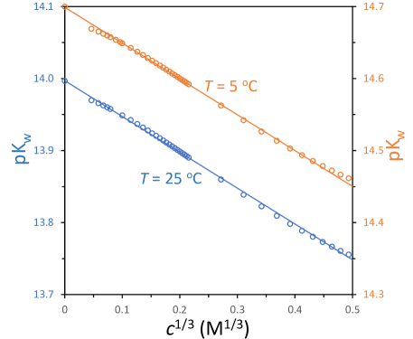
Figure 1: The effect of salt concentration on the water autodissociation constant, pK_w, at temperatures 5 and 25 ${}^{\circ}\text{C}$. Data extracted from commercial software, and lines according to Eq. (44) with $2/\ln\left(10\right)\,b\!=\!0.50$ (for $c_{\infty}\!=\!0$, $\text{pK}\mathrm{{}_{w,dil.}}\!=\!14.0$ for 25 ${}^{\circ}\text{C}$, and $\text{pK}\mathrm{{}_{w,dil.}}\!=\!14.7$ for 5 ${}^{\circ}\text{C}$). A lower pK_w implies that K_w is higher, thus concentrations of OH- and H3O+ are higher.

A separate topic to finally address in this section is the heat associated with such reactions, for instance of water association/dissociation. This heat is well known as the heat liberated when acid and base are mixed, and even when an acid or base is diluted. This is different from the heat of dilution due to the Coulombic interactions between ions discussed in ref. [11] which does not require chemical reactions. So we have an acid solution (volume $V\mathrm{{}_{A}}$ and a proton concentration $[\ce{H+}\mathrm{{}_{A}}]$), and a base solution ($V\mathrm{{}_{B}}$ and OH–concentration $[\ce{OH-}\mathrm{{}_{B}}]$). To simulate dilution of an acid or base with water, we set H+ or OH- to zero in either of these volume. After mixing, the concentration of cations minus that of anions equals the concentration difference of OH- minus H+. Thus, $V\mathrm{{}_{B}}[\ce{OH-}]\mathrm{{}_{B}}-V\mathrm{{}_{A}}[\ce{H+}]\mathrm{{}_{A}}=V\mathrm{{}_{tot}}\left([\ce{OH-}]-[\ce{H+}]\right)$, where $V\mathrm{{}_{tot}}=V\mathrm{{}_{A}}+V\mathrm{{}_{B}}$. This equation can be combined with Eq. (43) where $c_{\infty}$ equals the concentration of regular cations and H+-ions after mixing. So we have two equations and the two unknowns [H+] and [OH-], and that problem can be solved. How many molecules of water are now formed? This follows from the difference between total number of H+-molecules initially ($V\mathrm{{}_{A}}[\ce{H+}]\mathrm{{}_{A}}$) and after mixing ($V\mathrm{{}_{tot}}[\ce{H+}]$), and this decrease equals the number of OH- that reacts away, and equals the number of water molecules formed. With the enthalpy of formation of water from H+ and OH- at approx. $-56$ kJ/mol at $25^{\circ}$C, we calculate that the mixing of 1 L of an 1 M acid solution and 1 L of 1 M base solution, leads to the heating of the mixture with 6.7 ^∘C (heat capacity of water $\rho c\mathrm{{}_{p}}\!=\!4.2$ MJ/m³/K. With every factor of 10 lowering of concentration of both solutions, the temperature change goes down by the same factor. If one solution is kept at 1 M, and the other is more and more diluted before mixing, the temperature change after mixing, also drops to zero. Ultimately, when we simply mix an acid such as HCl or base such as NaOH with an equal volume of pure water, this does not lead to a temperature change from the water self-ionization reaction.

8 From Boltzmann’s law to chemical equilibrium of a reaction

8.1 Lattice gas statistics

It is interesting to make an analysis based on Boltzmann’s famous law for the entropy of a system

$$\textbf{S}=k\mathrm{{}_{B}}\ln W$$ (45)

where S is entropy and W is the number of microscopic configurations. If we assume there are N positions for a molecule to be, and M molecules, then the number of ways to arrange this, is

$$W=\frac{N!}{M!\left(N\!-\!M\right)!}\,.$$ (46)

Making use of Stirling’s approximation, valid for sufficiently large N and M, $\ln N!\sim N\ln N-N$, we arrive at

$$\textbf{S}/k\mathrm{{}_{B}}=N\ln N-M\ln M-\left(N-M\right)\ln\left(N-M\right)\,.$$ (47)

We now change from entropy of a system, S, to the free energy density, $f=-T\textbf{S}/V$, where V is volume. We also use $c\mathrm{{}_{max}}\cdot N\mathrm{{}_{av}}=N/V$ and $c\cdot N\mathrm{{}_{av}}=M/V$, and obtain

$$f=RT\left(c\ln\frac{c}{c\mathrm{{}_{max}}-c}-c\mathrm{{}_{max}}\ln\frac{c\mathrm{{}_{max}}}{c\mathrm{{}_{max}}-c}\right)\,.$$ (48)

For low values of $c$ relative to $c\mathrm{{}_{max}}$, Eq. (48) simplifies to

$$f=RT\left(c\ln\frac{c}{c\mathrm{{}_{max}}}-c\right)\,.$$ (49)

We can calculate the osmotic pressure, $\Pi$, according to $\Pi=c\partial f/\partial c-f$ (assuming only one component), and obtain

$$\Pi=cRT$$ (50)

which is the Ideal Gas law, which we here derived based on Eq. (45). Using the Gibbs-Duhem equation, $\partial\Pi/\partial c_{i}=c_{i}\cdot\partial\mu_{i}/\partial c_{i}$ (in case of only one component), we can integrate from a reference concentration $c\mathrm{{}_{ref}}$ (where $\overline{\mu}_{i}=\overline{\mu}_{\text{ref},i}$) to $c_{i}$, and then obtain from Eq. (50)

$$\overline{\mu}_{i}=\overline{\mu}_{\text{ref},i}+RT\int_{c\mathrm{{}_{ref}}}^{c_{i}}{c_{i}}^{-1}\text{d}c_{i}=\overline{\mu}_{\text{ref},i}+RT\ln\frac{c_{i}}{c\mathrm{{}_{ref}}}$$ (51)

which are exactly the first two terms of Eq. (1), here derived based on Eq. (45).

We can return to Eq. (48), implement a site occupancy, $\theta=c/c\mathrm{{}_{max}}$ and replace $c\mathrm{{}_{max}}$ by $1/\nu$, just as in Eq. (21). We then obtain

$$f=RT\cdot\nu^{-1}\cdot\left(\theta\ln\theta+\left(1-\theta\right)\ln\left(1-\theta\right)\right)$$ (52)

which appears as if we have an entropy term ‘$\theta\ln\theta$’ both for the occupied and for the free (available, unoccupied) sites, though of course there is no physical entity occupying the free sites.

If we evaluate Eq. (52) to derive the osmotic pressure, we obtain the elegant expression

$$\Pi_{i}=-RT\cdot\nu^{-1}\cdot\ln\left(1-\theta\right)$$ (53)

which in the dilute limit simplifies to the Ideal Gas law, Eq. (50), but at higher concentration increases faster than linearly.

We can evaluate Eq. (53) using the Gibbs-Duhem equation, which leads to

$$\overline{\mu}_{i}=\overline{\mu}^{*}_{\text{ref},i}+RT\ln\theta_{i}-RT\ln\left(1-\theta_{i}\right)$$ (54)

where $\overline{\mu}^{*}_{\text{ref},i}=\overline{\mu}_{\text{ref},i}-RT\ln\left(\theta\mathrm{{}_{ref}}/\left(1-\theta\mathrm{{}_{ref}}\right)\right)$. The last term in Eq. (54) is the same as the excess term proposed in Eq. (21) for the Langmuir isotherm, with here a derivation given of that term (for a single component).

In summary, in this section we developed equations for the ideal gas, and for non-dilute conditions, based on the concept (model) of a fixed number of positions where a molecule can either reside or not (lattice approach). The ideal gas expression (dilute limit) does not depend on this model but is generally valid: in the dilute limit, what else is possible for osmotic pressure than to be linearly dependent on concentration? However, the non-dilute expressions are based on this artificial model of molecules occupying discrete positions. This is likely a good approach when solutes indeed adsorb to distinct surface sites, but to describe the movements of ions in solution, this is not a correct approach, and various expressions relating to the Carnahan-Starling equation for hard sphere mixtures, are much better. This concludes our analysis of a lattice gas, in the dilute limit, and for non-dilute conditions. The analysis was made for a single solute (molecule) and without interactions between them. We can extend this theory, which then leads to expressions where many types of solutes are jointly considered, and intermolecular interaction energies are included, such as summarized in Eqs. (1) and (2) by the contribution $\overline{\mu}_{\text{mm},i}$.

8.2 From free energy to chemical equilibrium of a reaction

It is quite interesting that at chemical equilibrium an equation such as Eq. (40) describes the relationship between the concentrations of molecules that react with one another. And we know it should also hold in multi-component systems, with multiple types of molecules. Let us demonstrate this again based on minimization of the free energy in a closed system. We consider as an example three molecules, A, B and C, that can convert into one another, thus $\nu_{\mathrm{{}_{A}}}\text{A}\leftrightarrow\nu_{\mathrm{{}_{B}}}\text{B}\leftrightarrow\nu_{\mathrm{{}_{C}}}\text{C}$. In this section, stoichiometric factors $\nu_{i}$ are positive numbers, for all species, which is different from the approach in the previous section. From integration of Eq. (51), we obtain for the free energy density

$$f=RT\sum_{i}\left(c_{i}\ln\frac{c_{i}}{c\mathrm{{}_{ref}}}-\left(c_{i}-c\mathrm{{}_{ref}}\right)\right)+\sum_{i}\overline{\mu}_{\text{ref},i}\left(c_{i}-c\mathrm{{}_{ref}}\right)\,.$$ (55)

This expression for $f$ is different from Eq. (49) because of the recalculation via osmotic pressure and chemical potential, but in a practical calculation they will lead to the same result. Eq. (55) is valid for a multicomponent mixture, but only includes ideal entropy (dilute limit) and the reference term. The analysis can always be extended with extra contributions.

The total ‘equivalent concentration’ is given by $c\mathrm{{}_{eq}}=\sum_{i}c_{i}/\nu_{i}$, where we sum over the three molecules A, B, and C. For a closed system this equivalent concentration is constant. At chemical equilibrium, the free energy, $f$, is at a minimum, with the constraint of this equivalent concentration being constant, i.e., independent of the extent of the reactions. If we implement $c\mathrm{{}_{eq}}$ in Eq. (55), energy $f$ is only a function of the concentrations of A and B. Because we are at the minimum, both $\partial f/\partial c_{\mathrm{{}_{A}}}=0$ and $\partial f/\partial c_{\mathrm{{}_{B}}}=0$ (with the other concentration unchanged in the differentiation).

If we make the first differentiation, we arrive at

$$\nu_{\mathrm{{}_{A}}}\left(\ln\frac{c_{\mathrm{{}_{A}}}}{c\mathrm{{}_{ref}}}+\mu_{\mathrm{{}_{ref,A}}}\right)-\nu_{\mathrm{{}_{C}}}\left(\ln\frac{c_{\mathrm{{}_{C}}}}{c\mathrm{{}_{ref}}}+\mu_{\mathrm{{}_{ref,C}}}\right)=0$$ (56)

and thus the relation between the concentrations of A and C is

$$\left(\frac{c_{\mathrm{{}_{A}}}}{c\mathrm{{}_{ref}}}\right)^{\nu_{\mathrm{{}_{A}}}}\cdot\left(\frac{c\mathrm{{}_{ref}}}{c_{\mathrm{{}_{C}}}}\right)^{\nu_{\mathrm{{}_{C}}}}=K=\exp\left\{\nu_{\mathrm{{}_{C}}}\mu_{\mathrm{{}_{ref,C}}}-\nu_{\mathrm{{}_{A}}}\mu_{\mathrm{{}_{ref,A}}}\right\}$$ (57)

and a similar equation links the concentration of B to that of A or C. Thus, an equilibrium such as Eq. (40) follows from a minimization of free energy, also in multi-component systems. The analysis can be extended to include non-ideal effects, leading to an equation such as Eq. (41). Thus, a direct analysis based on equality between the chemical potential of all reactants on one side, and products on the other side, is in line with the outcome of a minimization of free energy.

9 Chemical equilibrium involving ions and a charged material

When a porous material is charged, which is the case with most membranes that are used for water desalination, the situation becomes even more interesting. We now assume that in solution, outside the membrane, ions behave ideally, i.e., only the term $\ln c_{\infty,i}$ needs to be considered for the chemical potential. When a porous material is charged, we always have anions and cations, and the simplest case is a 1:1 salt. For an ion absorbing in a charged porous material, we have the effects of solubility, ion volume, just as in Eq. (19), and the electrical potential, $\mu_{\text{el},i}=z_{i}\phi$. The partitioning due to the electrical potential is called a Donnan effect, and thus we arrive at

$$c_{\text{m},i}=c_{\infty,i}\Phi_{\text{aff},i}\Phi_{\text{exc},i}\Phi_{\text{D},i}$$ (58)

with

$$\Phi_{\text{D},i}=e^{-z_{i}\phi\mathrm{{}_{D}}}$$ (59)

where the Donnan potential, $\phi\mathrm{{}_{D}}$, is the electrical potential inside the porous material, $\phi\mathrm{{}_{m}}$, minus outside, $\phi_{\infty}$, thus $\phi\mathrm{{}_{D}}=\phi\mathrm{{}_{m}}-\phi_{\infty}$. Just as for the isotherm modeling, we define all concentrations based on the pore volume, i.e., the volume accessible to ions and solvent.

Eq. (58) must be set up for both ions, anion and cation, and must be combined with one more equation, for charge neutrality in the membrane, given by

$$\sum_{i}z_{i}c_{\text{m},i}+X=0$$ (60)

where X is the charge density of the material, expressed as a concentration, i.e., in moles per volume, and just as for ion concentrations, this volume is the water-filled pore fraction. This charge density can be positive (for instance for a membrane for reverse osmosis at low pH) or negative (reverse osmosis membrane at high pH). When $\Phi_{\text{exc},i}$ is a constant (just like $\Phi_{\text{aff},i}$ generally is), i.e., not dependent on ion concentrations, then these equations can be solved jointly without much trouble for any mixture of ions, for a given value of membrane charge, X, by inserting Eq. (58) for all ions into Eq. (60), and solving for the Donnan potential, $\phi\mathrm{{}_{D}}$, after which plugging that result back in Eq. (58) gives us all concentrations in the membrane. This is the same when membrane charge is a function of the Donnan potential. For instance, for a membrane that is acidic (i.e., negatively charged, and the more so at higher pH), i.e., it is ionizable, we can implement in Eq. (60) that $X=X\mathrm{{}_{max}}/\left(1+[\ce{H+}]\mathrm{{}_{m}}/K\mathrm{{}_{A}}\right)$, where both $X$ and $X\mathrm{{}_{max}}$ are negative numbers. The proton concentration in the membrane is also described by Eqs. (58) and (59), and for protons and hydroxyl ions typically both $\Phi_{\text{exc},i}$ and $\Phi_{\text{aff},i}$ are set to unity (i.e., to 1), resulting in the Boltzmann relationship

$$c_{\text{m},i}=c_{\infty,i}e^{-z_{i}\phi\mathrm{{}_{D}}}\,.$$ (61)

Thus, also for an ionizable membrane, i.e., when membrane charge is a function of pH, which in turn is a function of charge, ion concentrations, etc., the resulting equations can be readily solved after iteratively solving for $\phi\mathrm{{}_{D}}$.

We now continue with a 1:1 salt as an example, though in principle any mixture of ions can considered. The expression for charge neutrality becomes

$$c_{\text{m},+}-c_{\text{m},-}+X=0$$ (62)

and the equation to be solved in $\phi\mathrm{{}_{D}}$ is

$$c_{\infty}\Phi_{+}e^{-\phi\mathrm{{}_{D}}}-c_{\infty}\Phi_{-}e^{+\phi\mathrm{{}_{D}}}+\frac{X\mathrm{{}_{max}}}{1+[\ce{H+}]_{\infty}e^{-\phi\mathrm{{}_{D}}}/K\mathrm{{}_{A}}}=0$$ (63)

where $\Phi_{i}$ is the product of the affinity and excess partition coefficients, $\Phi_{i}=\Phi_{\text{aff},i}\Phi_{\text{exc},i}$, and where $c_{\infty}$ is the salt concentration of the 1:1 salt. (We neglect a contribution of H+ and OH- to the charge balance in solution and in the membrane, though [H+] does influence the membrane charge.) Now, to simplify, we assume this overall partition coefficient, $\Phi_{i}$, is the same for the two ions. We then obtain

$$2c_{\infty}\,\Phi_{i}\,\sinh\phi\mathrm{{}_{D}}=\frac{X\mathrm{{}_{max}}}{1+[\ce{H+}]_{\infty}e^{-\phi\mathrm{{}_{D}}}/K\mathrm{{}_{A}}}$$ (64)

where $\sinh(x)=\text{\textonehalf}\left(\exp(x)-\exp(-x)\right)$. If we now assume that the membrane charge is fixed (for instance because we work at high pH and/or $K\mathrm{{}_{A}}$ is sufficiently high), we obtain

$$2c_{\infty}\,\Phi_{i}\,\sinh\phi\mathrm{{}_{D}}=X$$ (65)

where index ‘max’ is left out. We can rewrite Eq. (65) to

$$\phi\mathrm{{}_{D}}=\sinh^{-1}\left(\frac{X}{2\Phi_{i}c_{\infty}}\right)$$ (66)

where $\sinh^{-1}$ is the inverse of the $\sinh$-function (also written as asinh, or arcsinh), and thus we have an explicit solution for $\phi\mathrm{{}_{D}}$ as function of salt concentration and membrane charge. The Donnan potential, $\phi\mathrm{{}_{D}}$, and membrane charge density, X, have the same sign.

Each of the above equations, from Eq. (63) to Eq. (66), is an extended isotherm. It is also part of an electrical double layer (EDL) model. An EDL model, or EDL theory, describes the Donnan potential as function of the charge of the material, and based on that, the concentrations of all ions inside a material. Thus an EDL model is an extension of an isotherm, which is set up for neutral solutes. Both isotherms and EDL models describe the relationship between the concentrations of solutes i in two phases, when we have chemical equilibrium between these two phases. An EDL model is more extended than an isotherm because it has to deal with solutions with ions of all kind of charges, not only neutral molecules, and also includes the charge balance for each phase (each phase overall is charge neutral). Thus, the concept of an EDL model refers to a set of equations that describes the structure of a charged interface in contact with an electrolyte solution containing ions, including in the description the charge and potential of the interface.

Based on Eq. (66) we can calculate the anion and cation concentrations inside the charged porous material, again defined per unit pore volume. But first we calculate the total ions concentration, $c\mathrm{{}_{T,m}}=c\mathrm{{}_{m,ct}}+c\mathrm{{}_{m,co}}$, which results in

$$c\mathrm{{}_{T,m}}=c_{\infty}\Phi_{i}\left(e^{\phi\mathrm{{}_{D}}}+e^{-\phi\mathrm{{}_{D}}}\right)=2c_{\infty}\Phi_{i}\,\cosh\phi\mathrm{{}_{D}}=\sqrt{X^{2}+\left(2\Phi_{i}c_{\infty}\right)^{2}}$$ (67)

where we used the conversion $\cosh(\sinh^{-1}(x))=\sqrt{x^{2}+1}$, and implemented Eq. (66). Eq. (67) shows that the total ions concentration depends on X, does not depend on the sign thereof, and is always larger than $|X|$ (the use of $|\dots|$ refers to the magnitude, i.e., absolute value of the argument). The concentration of counterions (ct) is larger than $|X|$, and the concentration of coions (co) much smaller. They are given by

$$c\mathrm{{}_{m,ct}}=\text{\textonehalf}\left(c\mathrm{{}_{T,m}}+|X|\right)\hskip 8.53581pt,\hskip 8.53581ptc\mathrm{{}_{m,co}}=\text{\textonehalf}\left(c\mathrm{{}_{T,m}}-|X|\right)\,.$$ (68)

We can check validity of Eq. (68) by multiplying $c\mathrm{{}_{m,ct}}$ with $c\mathrm{{}_{m,co}}$, which should have the result $c_{\infty}^{2}\Phi_{i}^{2}$. Indeed, implementing Eq. (67) in Eq. (68) and multiplying the two concentrations, results in the required outcome. Thus, there are counterions in a charged membrane at a concentration larger than the charge density, $|X|$, and coions at a much lower concentration. The concentration of coions is very important as it often determines the salt transport rate in a membrane process. Thus, it is important to exactly know this concentration. Studies of the EDL help to find the exact value of this coion concentration.

Another property of importance is the hydrostatic pressure inside the material, $P^{\text{h}}$, that pushes the charged material outward, against the outside hydrostatic pressure. This pressure difference equals the difference in osmotic pressure between inside and outside, $\Delta\Pi$, and for a 1:1 salt, this difference is $\Delta\Pi=RT\cdot\left(c\mathrm{{}_{T,m}}-2c_{\infty}\right)$, which can be solved based on Eq. (67), and then we also know $\Delta P^{\text{h}}=P^{\text{h,inside}}-P^{\text{h},\infty}$. For a low external hydrostatic pressure, low charge X, and low $\Phi_{i}$, it is possible that negative pressures develop inside the porous material.

From Eq. (62) onward we considered a solution with one anion and one cation inside a charged porous material. In Ch. 2 of ref. [3] a related problem is described where a monovalent cation, Na+, and a divalent cation, Ca^2+, absorb from a mixed electrolyte solution into a negatively charged porous material. Observations are, and theory predicts this as well, that when the mixed electrolyte solution is diluted, thereby keeping the ratio of Ca^2+ over Na+ in solution constant, that monovalent cations Na+ desorb from the porous material, but the divalent cations do not. They even absorb more. This can be explained using the balances presented above, without the need to include partition coefficients for affinity or volume. In Eq. (63) we only must include the extra divalent cation. The membrane charge can be set to a fixed value.

Ion volume effects in porous materials, and resulting selectivity. There are expressions for $\mu_{\text{exc},i}$ for ions (or other molecules) in a porous material that take into account their size, their concentration and that of other solutes, and how dense is the porous material. In such a description the porous material is characterized by its porosity, and by a characteristic pore dimension, $h\mathrm{{}_{p}}$, which is the ratio of all pore volume, over the internal surface area. This is the area of contact inside the porous structure between the liquid-filled pores and the matrix material. It is the inverse of a factor $a\mathrm{{}_{L}}$ which is a liquid-solid specific area, i.e., a contact area per unit liquid phase volume, a relevant parameter in chemical engineering calculations.

In case the absorbing solutes do not interact with one another, but only with the porous material, and if we assume the solutes to be spherical, then the contribution to the chemical potential is $\mu_{\text{exc},i}=\text{\textonehalf}\alpha^{\prime}$ where $\alpha^{\prime}$ is the size of the solute divided by the specific pore dimension, $h\mathrm{{}_{p}}$, see Ch. 4 in ref. [3]. This expression is valid for values of $\alpha^{\prime}$ between 0 and 1. We then arrive at a contribution to $\Phi_{i}$ that is independent of the concentration of ions in the pores.

However, there are no simple expressions for the case that we simultaneously have interactions of the ions with the porous material and with each other, in which case $\Phi_{i}$ becomes a function of ion concentrations. One calculation reported in Ch. 4 of ref. [3] is of a porous material with porosity 50 vol%, and in these pores 20 vol% of space is occupied by smaller and larger particles, with the larger particles 20% larger in size than the smaller ones. In solution outside the material they have the same concentration. It turns out that inside the pores the number of smaller particles is $4.4\times$ that of the larger particles, i.e., a selectivity towards the smaller particles (only 20% smaller in size than the larger ones) of a factor 4.4. Thus, these volume exclusion effects can be very significant.

10 Conclusions

The chemical potential of an ion is an important concept to understand absorption of ions from an electrolyte solution into neutral and charged materials such as absorbents and membranes. This is relevant for processes where ion absorption, transport, and exchange play a key role. For neutral molecules and materials, at chemical equilibrium the concept of an isotherm is of importance, which for charged molecules and materials is extended to electrical double layer theory. The chemical potential has many contributions, and in a calculation of the distribution of ions across an interface eventually all terms depend on the concentration and on temperature. For ions in solution, deviations from ideal behaviour are often classified as activity coefficients, and they are due to ion volume effects and ion-ion Coulombic interactions. These contributions lead to an osmotic coefficient less than one, and thus the osmotic pressure of a solution is less than predicted by the ideal contribution only. In a porous material, the non-zero volume of solutes is also a contribution to the chemical potential, making it more difficult for larger ions to reside in a porous material than smaller ones.

References

- [1] P.M. Biesheuvel, “Two-fluid model for the simultaneous flow of colloids and fluids in porous media,” J. Colloid Interface Sci. 355, 389–395 (2011).
- [2] E. Spruijt and P.M. Biesheuvel, “Sedimentation dynamics and equilibrium profiles in multicomponent mixtures of colloidal particles,” J. Phys. Condens. Matter 26, 075101 (2014).
- [3] P.M. Biesheuvel and J.E. Dykstra, Physics of Electrochemical Processes, ISBN:9789090332581 (2020).
- [4] P.M. Biesheuvel, S. Porada, M. Elimelech, and J.E. Dykstra, “Tutorial review of reverse osmosis and electrodialysis,” J. Membr. Sci. 647, 120221 (2022).
- [5] A. Einstein, “Investigations on the theory of brownian movement,” Dover (1956). (This book is a reproduction of the translation into English from 1926, which is based on papers published between 1905 and 1908.)
- [6] E.M. Kimani, A.J.B. Kemperman, W.G.J. van der Meer, and P.M. Biesheuvel, “Multicomponent mass transport modeling of water desalination by reverse osmosis including ion pair formation,” J. Chem. Phys. 154, 124501 (2021).
- [7] J.E. Dykstra, A. ter Heijne, S. Puig, and P.M. Biesheuvel, “Theory of transport and recovery in microbial electrosynthesis of acetate from CO2,” Electrochim. Acta 379, 138029 (2021).
- [8] S. Castaño Osorio, P.M. Biesheuvel, E. Spruijt, J.E. Dykstra, and A. van der Wal, “Modeling micropollutant removal by nanofiltration and reverse osmosis membranes: considerations and challenges,” Water Research 225, 119130 (2022).
- [9] S.R. Milner, “The virial of a mixture of ions,” Phil. Mag. 23, 551–578 (1912).
- [10] S.R. Milner, “The effect of interionic forces on the osmotic pressure of electrolytes,” Phil. Mag. 25, 742–751 (1913).
- [11] P.M. Biesheuvel, “The activity coefficient of z:1 ionic solutions scales with the cube root of salt concentration,” arXiv:2012.12194 (2020).
-
[12]
N. Bjerrum, “The dissociation of strong electrolytes,” Fysisk Tids. 15 59 (1916).
Available in English translation. Published in German as:
N. Bjerrum, “Die Dissoziation der starker Elektrolyte,” Z. Elektrochem. 24, 321–328 (1918). -
[13]
N. Bjerrum, “On the activity coefficient for ions,” Medd. Vetenskapsakad. Nobelinst. 5 1 (1919). Available in English translation. Published in German as:
N. Bjerrum, “Der Aktivitätskoeffizient der Ionen,” Z. Anorg. Chem. 109, 275–292 (1920). - [14] M.R. Wright, “An introduction to aqueous electrolyte solutions,” Wiley, Chichester (2007).