Spatially-resolved Thermometry from Line-of-Sight Emission Spectroscopy via Machine Learning

Abstract

A methodology is proposed, which addresses the caveat that line-of-sight emission spectroscopy presents in that it cannot provide spatially resolved temperature measurements in nonhomogeneous temperature fields. The aim of this research is to explore the use of data-driven models in measuring temperature distributions in a spatially resolved manner using emission spectroscopy data. Two categories of data-driven methods are analyzed: (i) Feature engineering and classical machine learning algorithms, and (ii) end-to-end convolutional neural networks (CNN). In total, combinations of fifteen feature groups and fifteen classical machine learning models, and eleven CNN models are considered and their performances explored. The results indicate that the combination of feature engineering and machine learning provides better performance than the direct use of CNN. Notably, feature engineering which is comprised of physics-guided transformation, signal representation-based feature extraction and Principal Component Analysis is found to be the most effective. Moreover, it is shown that when using the extracted features, the ensemble-based, light blender learning model offers the best performance with RMSE, RE, RRMSE and R values of 64.3, 0.017, 0.025 and 0.994, respectively. The proposed method, based on feature engineering and the light blender model, is capable of measuring nonuniform temperature distributions from low-resolution spectra, even when the species concentration distribution in the gas mixtures is unknown.

1 Introduction

Emission spectroscopy is a popular gas-thermometry technique, extensively utilized in the fields of remote sensing [1] and combustion diagnostics [2], among others. It naturally relies on the line-of-sight property, since a spectrum is obtained through the convolution of the emission signals along the light path. Thus, in the context of thermometry, only a single average temperature measurement, rather than a spatially resolved temperature profile, can be obtained [3]. Limited by this caveat, the use of emission spectroscopy-based thermometry is constrained to scenarios involving roughly homogeneous gases.

Although advanced methods, such as tomographic spectroscopy [4] and laser-induced fluorescence [5] are able to provide spatially resolved temperature measurements in the gaseous phase, emission spectroscopy is much simpler in terms of the hardware requirements, cheaper, and easier to use. Moreover, emission spectroscopy can be extended to hyperspectral imaging, which is a core technology in remote sensing [6, 7]. Therefore, the development of advanced estimation methods for spatial temperature distributions from line-of-sight emission spectra could support the development of a powerful thermometry tool for use in both research and development applications.

The motivation behind this work is that the spatial nature of the temperature distribution is not lost during the scanning process, but rather it is encoded within the emission spectrum representation. Figure 1 illustrates this point. Suppose that the light path develops along a homogenous gas, where the mole fraction of CO₂ is 0.1, divided into two segments with temperatures of 500 K and 1500 K, respectively. Assume that two spectrometers are respectively placed at either end of the light path to capture the spectral information. As shown in Figures 1(a) and (b), the temperature profiles along the light path, which will be used to capture the associated spectra, are, of course, the inverse of each other. The HITRAN Application Programming Interface (HAPI) [8] was used to simulate the spectra for each of the two cases. Figures 1 (c) and (d) show both the corresponding high-resolution spectra (resolution of 0.1 $cm^{-1}$), and the low-resolution version (resolution of 4 $cm^{-1}$), after the tuning of the triangular slit functions. It is evident that the two spectra are totally different in terms of appearance, irrespective of the choice of resolution. Indeed, the primary variable controlling their appearance is the ordering of two temperature segments, i.e., 500 K and 1500 K. This observation supports the hypothesis that temperature information is encoded rather than eliminated during the acquisition process of the emission spectrum.

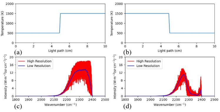
Figure 1: Comparison of spectra captured from the two ends of the same light path. (a) Temperature profile along the light path from left (500 K) to right (1500 K); (b) Temperature profile along the light path from right (500 K) to left (1500 K); (c) Emission spectrum generated from the light path in (a); (d) Emission spectrum generated from the light path in (b). Both high and low resolution spectra is visualized in (c) and (d).

A pioneering idea to realize spatially resolved temperature measurements from line-of-sight data is inverse modelling by using regularization of profile smoothness [9, 10, 11]. In this method, a radiative model is used in order to approximate the test spectrum by varying the spatial distribution of temperature. By monitoring the consistency between the estimated and test spectra, the quality of the measured spatially resolved temperature distributions can be assessed. However, since spectrum intensity does not only depend on temperature, but also the concentration of the species of interest, to avoid divergence of temperature measurement, the concentration distribution is supposed to be known in some studies [9, 11]. Moreover, the hyperparameters of the utilized optimization algorithms often require careful adjustment, in order to allow the matching of measurements with the ground truth [10, 11]. Unfortunately, neither prior knowledge of concentration nor the ground truth of the temperature distribution, which is the task at hand in this research, are available in practice, and thus, there is no direct information to support adjustment of the associated hyperparameters.

The inherent difficulties in extracting and interpreting the latent spatial temperature information within line-of-sight emission spectra using the physics-driven perspective, naturally suggest exploring the power of data-driven methods. A number of studies attempted the use of machine learning in the context of such measurements [12, 13]. However, they were limited in using Multilayer Perceptrons (MLP) [14]. Recent advances in machine learning (ML) and deep learning (DL), e.g., building on the paradigms of Convolutional Neural Networks (CNN) [15], and blending methods [16], may be able to improve measurement accuracy. Moreover, the length of the acquired spectral measurements translates to a high dimensional representation of the associated information, which could be problematic, when directly used with classical ML algorithms. This problem is termed the curse of dimensionality [17], and relates to the increase in the dimensionality of the solution space, leading to sparse data coverage, which subsequently affects the quality of the ML solution. A means to tackle this is extracting lower dimensional, compact features to represent the high dimensional information, also termed as Feature Engineering (FE).

This research systematically addresses the challenge of recovering spatial temperature information from line-of-sight emission spectra measurements using data-driven modelling approaches. The contributions of the work are summarized as follows:

1. A variety of feature engineering approaches were considered. Knowledge of the physical model of the process was used to transform the spectra, and next, fifteen feature groups were extracted to succinctly describe their characteristics. A wrapper-based feature selection method, i.e., utilizing an MLP as the means to quantify feature quality, was used to select the most informative features, which were found to be the combination of physics-guided transformation, signal representation-based feature extraction [18], and Principal Component Analysis [19].

2. Extensive exploration of classical machine learning algorithms was pursued. In addition to the MLP algorithm, a variety of methods, including Radial Basis Function Networks [20], Gaussian Process Regression [21], etc. were attempted. In total, fifteen machine learning models were trained and tested. It was found that the best performance was obtained with the light blender model, a two-stage ensemble learning model, realized by a blending method [16], which produced superior results, compared to the state-of-the-art [12, 13].

3. DL/CNN methods were explored in detail. We compared the performance of traditional ML methods coupled with feature engineering, against a number of end-to-end DL algorithms, such as Resnet [22] and Shuffle Net [23]. It was found that the combination of raw spectra inputs and CNN was not able to match the excellent performance of the combination of feature engineering and ML. This demonstrates that feature engineering can play an important role in certain application domains, including the problem under consideration in this research.

2 Methodology

Figure 2 provides an overview of the overall system methodology. It basically includes two steps: (a) data generation, i.e., using the physical (forward) model to synthetize emission spectra, and (b) data-driven modelling, where the generated data is used to train and test the performance of FE+ML/DL models.

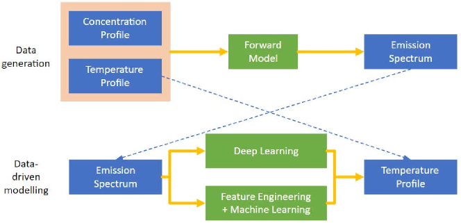
Figure 2: Overview of research methodology

2.1 Forward Model and data generation

2.1.1 Physical forward model

In order to synthese spectra for the purpose of training and testing machine learning models, a forward emission spectroscopy model was constructed, based on the well-established HITEMP2010 database [24], and its simulation platform, HAPI [8].

For the purpose of generating spectra from nonuniform temperature profiles, we first discretized the light path, going through a gas cloud (such as a flame), into n segments, as shown in Figure 3. Thus, nonuniform temperature and concentration profiles could be modelled within these segments.

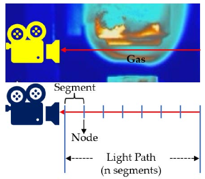
Figure 3: Schematic diagram of light path division

Following the theory of spectroscopy [25], the intensity at the exit of a segment is the sum of the emission of the current segment and the transmission of the radiation from the previous segments:

$$I_{v,o}=\epsilon_{v}I_{v,B}+t_{v}I_{v,i}$$ (1)

where $I$, $\alpha$, $t$ are the intensity, emissivity, and transmissivity, respectively. The subscripts $v$,$B$,$i$, and $o$ relate to the frequency, Black-body radiance, incident and outlet nodes of the segment, respectively. According to the Beer-Lambert law [25], transmissivity can be expressed by:

$$t_{v}=exp(-k_{v}l)$$ (2)

where $k_{v}$ is the absorption coefficient $(cm^{-1})$, and $l$ is the length of the light path segment (cm). The sum of transmissivity $t$ and absorptivity $\alpha$ is equal to 1, when scattering and reflection are neglectable, i.e.,

$$t_{v}+\alpha_{v}=1$$ (3)

Let us consider that the gas cloud is at thermal equilibrium. By following Kirchhoff’s law of thermal radiation [25] that emissivity equals to absorptivity, and substituting Eqs.2-3 into Eq.1, we get:

$$I_{v,o}=(1-exp(-k_{v}l))I_{v,B}+exp(-k_{v}l)I_{v,i}$$ (4)

Moreover, the black-body radiance can be modeled by Plank’s law [26]:

$$I_{v,B}=\frac{2hv^{3}}{c^{2}(exp(\frac{hv}{k_{B}T})-1)}$$ (5)

where h is the Plank constant, $k_{B}$ is the Boltzmann constant, $c$ is the light speed, and $T$ is the temperature. Then, the absorption coefficient, $k_{v}$, of gas species $j$ is given by:

$$k_{v,j}=s_{v,j}(T)\phi_{v}(T,p)\frac{pX_{j}}{k_{B}T}$$ (6)

where s is the line intensity per molecule ($(cm)^{-1}/(molecule*cm^{-2})$), which is a function of temperature, $\phi_{v}$ is the Voigt profile [27], which is a function of both pressure and temperature, and $p$ is the local pressure ($Pa$), and $X$ is the mole fraction. The total absorption coefficient can be simplified as the sum of the absorption coefficients of each species:

$$k_{v}=\sum k_{v,j}$$ (7)

Although high resolution spectra are better in providing precise information, low-resolution spectra, which are affected by blurring due to line broadening and the slit function of the instrument, are the norm in engineering measurements. A triangular function was used to simulate the instrument slit function as follows:

$$B(x)=\begin{cases}\begin{aligned} \frac{1-\frac{abs(v-v_{c})}{w}}{w}\qquad&abs(v-v_{c})\leq w\\ 0\qquad&abs(v-v_{c})>w\end{aligned}\end{cases}$$ (8)

where $w$ is the wing of the triangular function, which is set to 10 $cm^{-1}$, and $v_{c}$ is the center of the triangular function, in this work, the resolution of spectrum is 4 $cm^{-1}$.

By considering the aforementioned equations, a number of factors can be identified that hinder retrieval of spatially resolved temperature measurements. First, as observed in Eq.6, both temperature and species concentration affect the appearance of the spectrum. Thus, lack of prior information in regards to the species concentration increases the difficulty in retrieving the varying temperature profile along the light path. Second, as shown in Eq. 7, in the case of gas species mixtures, the total absorption coefficient is affected by the spectral characteristics of all species, thus, posing a further complication in estimating the temperature measurement information. Third, blurring due to various factors, including the instrument slit function of Eq. 8, reduces the quality of spectral information, increasing the ambiguity in temperature measurement. Last, temperature profile non-uniformity and lack of prior information in respect to the range of the temperature distribution complicate the extraction of patterns, governing the spectra.

2.1.2 Data generation

In this research, we focus on the paradigm of combustion. This is a suiTablescenario for spatially resolved temperature measurements with emission spectroscopy, because the high temperatures of the combustion process provide sufficient emission signals. Moreover, most practical combustion phenomena naturally possess nonuniform temperature distributions, which, in turn, require spatially resolved temperature measurements. In the data generation, the conditions, which occur in combustion were replicated, however, more complex situations were also considered. This was achieved by varying each of the four parameters, which affect the appearance and quality of the spectra, subsequently affecting temperature profile estimation, i.e., uncertainties in concentration, mixture of species, nonuniformities and range of temperature distribution, and spectral resolution. This methodology was followed to systematically assess the capabilities of ML/DL algorithms in tackling the temperature measurement problem. The detailed data configuration is described in the following paragraphs.

The gases considered were CO, CO₂ and H₂O, because of their importance in combustion applications. As previously mentioned, such gas mixtures also complicate temperature measurement estimation. Following [13], the wavebands selected were in the range of 1800-2500 $cm^{-1}$, which covers the emission bands of these three substances. The light path was set to be ten cm and divided into eleven segments, i.e., there were twelve nodes, with each segment being less than one cm in length. The relatively small segment length and the number of the segments suffice to validate the feasibility of measuring spatially resolved temperature measurements. Indeed, the number of segments may vary according to the requirements of the application. The dual-peak Gaussian function, commonly encountered in flames [28], was used as the base profile herein. The ideal dual-peak Gaussian function is given by:

$$\rho_{DG,j}=exp(-n(\frac{j-n}{4\sigma})^{2})+exp(-n(\frac{3(j-n)}{4\sigma})^{2})$$ (9)

where $\rho_{DG,j}$ is the density of dual-peak Gaussian profile at segment $j$, $n$ is the number of segments, $\sigma$ is the spread, which was empirically set to 16. The values of $\rho_{DG,j}$ were normalized in the range of (0,1). The feasible ranges of temperature and mole fraction can be obtained from the normalized density as follows:

$$T_{DG,j}=\rho_{DG,j,norm}(T_{max}-T_{min})+T_{min}$$ (10)

$$X_{DG,j}=\rho_{DG,j,norm}(X_{max}-X_{min})+X_{min}$$ (11)

where $\rho_{DG,j,norm}$ is the normalized basis height, $T_{DG,j}$ and $X_{DG,j}$ are, respectively, the temperature and mole fraction at segment j, $T_{max}$, $T_{min}$ and $X_{max}$, $X_{min}$ are, respectively, the maximum and minimum of temperature range and mole fraction range. The corresponding temperature range was set to 1500 K-3100 K, i.e., covering a broad interval of 1600 K, while the mole fraction range was set to 0.095-0.15, with examples of ideal generated profiles demonstrated in Figure 4 (a).

Next, the values of temperature and gas concentration in each segment were randomly varied in the ranges of ±300 K and ±0.015, respectively. Examples of temperature profiles generated by introducing such variations are shown in Figure 4 (b). It is evident that such variations have a significant impact on the shape of generated profiles. For instance, see Figure 4 (b), cases 1 and 2, which are generated from such profile configurations , do not exhibit the traditional shape of the dual peak Gaussian function. Rather, they resemble the shapes of trapezoidal and parabolic profiles, respectively. It should be emphasized that such profiles are also commonly observed in boundary-layer flow and flames [29, 30]. Given the light path discretization, a large variety of profile patterns can be generated, leading to higher spectral pattern complexity, thus increasing the difficulty in obtaining spatially resolved temperature measurements. In our experiments, we considered a spectral resolution of 4 $cm^{-1}$, although a resolution of 0.1 $cm^{-1}$ is practically realizable. The purpose behind this choice is that a lower resolution leads to higher spectral generation speed, reduced instrument costs, and also it increases the challenge of obtaining temperature measurements.

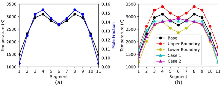
Figure 4: Temperature and concentration profiles. (a) Baseline– ideal profile, (b) Examples of temperature profiles, generated through random variation of the associated parameters.

In total, 28,000 spectra were generated. A sample profile is shown in Figure 5. Such a low-resolution spectrum comprises of 6799 emission lines. Compared to the high-resolution spectra of 0.1 $cm^{-1}$, also shown in the Figure, it is clear that low-resolution spectra is affected by blurring and is not able to capture finer spectral details.

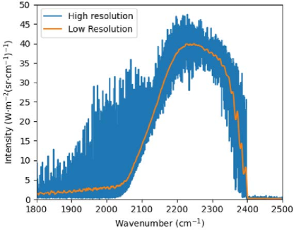
Figure 5: A sample of low-resolution spectrum.

2.2 Data-driven modelling

In the context of solving the inverse problem of line-of-sight emission spectroscopy, temperature parameters along the light path were estimated from the generated spectral dataset via data-driven modeling. Two types of data-driven modeling methods were considered: (i) feature engineering and classical machine learning algorithms; and (ii) raw spectra and CNN.

2.2.1 Feature engineering

Despite the substantial size of the generated spectra samples, the high dimensionality of the spectra, i.e., 6799 emission lines, would translate to a sparse sampling of the problem space, thus posing a challenge for machine learning algorithms. Therefore, feature engineering was performed on the raw spectra inputs, so as to extract informative features, thus reducing redundancy and problem dimensionality. First, the physics-guided, logarithmic transformation was used, so as to reduce the degree of nonlinearity of the mapping between spectra and temperature. Next, two types of feature extraction methods were used, i.e., extracting statistical and signal representation features, respectively. Principal Component Analysis (PCA) [19] was subsequently used to remove noise, and further reduce the dimensionality of features. In the following subsections, we briefly introduce the feature engineering operations.

Logarithmicic transformation. According to Eq.4 in the physical forward model, the absorption coefficient which contains the information of temperature is affected by an exponential function. This introduces nonlinearities in the associated temperature-spectrum mapping, which need to be resolved through the machine learning modelling. Applying the logarithmicic transformation [31] to the raw signals, assists by decreasing the mapping nonlinearities. This process is termed physics-guided transformation, since it is inspired by radiation physics.

Statistical features. Statistical features, such as first-, second- and higher-order statistics are often used to describe high-dimensional data [32, 33]. The list of time domain statistical parameters estimated from the emission spectra is shown in Table 1. Moreover, the Fast Fourier transform (FFT) was applied on the spectra, and extracted frequency domain features, as shown in Table 2. In total, 38 features were obtained, 23 from the time domain, with the remaining ten obtained from the frequency domain. In addition to extracting these features by considering the entire waveband (1800-2500 $cm^{-1}$), it is also possible to consider these features from the characteristic bands of the chemical substances. By characteristic band, we refer to the part of the spectral range, where the signal of one mixture component is dominant, with negligible contributions originating from the other components. For H₂O, CO and CO₂, such characteristic bands are the ranges of (1800 $cm^{-1}$, 1890 $cm^{-1}$), (2100 $cm^{-1}$, 2190 $cm^{-1}$), and (2310 $cm^{-1}$, 2400 $cm^{-1}$), respectively. Thus, three further set of 38 statistical features were also extracted from each of the three characteristic bands.

Table 1: Time domain features of the emission spectra

Features	Defination
Mean	$\bar{I}=\frac{1}{n}\sum_{i=1}^{n}I_{i}$,
	$i$ s the index of spectral signal, $n$=6799
Maximum	$I_{max}=max(I_{i})$
Minimum	$I_{min}=min(I_{i})$
Quartile 1	$I_{0.25*n}$, $I$ in ascending order
Quartile2 (median)	$I_{0.5*n}$, $I$ in ascending order
Quartile 3	$I_{0.75*n}$, $I$ in ascending order
Interquartile range	$I_{0.75*n}-I_{0.25*n}$
Standard deviation	$S=\sqrt{\frac{1}{n}\sum_{i=1}^{n}(I_{i}-\bar{I})^{2}}$
Variance	$S^{2}$
Skewness	$\frac{1}{n}\sum_{i=1}^{n}(\frac{I_{i}-\bar{I}}{S})^{3}$
Kurtosis	$\frac{1}{n}\sum_{i=1}^{n}(\frac{I_{i}-\bar{I}}{S})^{4}$
Inverse coefficient of variation	$\bar{I}/S$
Peak to peak	$I_{max}-I_{min}$
Zero cross rate	Number of signal sign changes
Root mean square	$RMS_{I}=\sqrt{\frac{1}{n}\sum_{i=1}^{n}I_{i}^{2}}$
Crest factor	$I_{max}/RMS_{I}$
Root mean square of difference	$S=\sqrt{\frac{1}{n-1}\sum_{i=1}^{n-1}(I_{i+1}-I_{i})^{2}}$
Root mean square of difference reciprocal	$S=\sqrt{\frac{1}{n-1}\sum_{i=1}^{n-1}\frac{1}{(I_{i+1}-I_{i})^{2}}}$
Mean of magnitude	$\frac{1}{n}\sum_{i=1}^{n}|I_{i}|$
Difference variance	$\frac{1}{n-1}\sum_{i=1}^{n-1}|I_{i+1}-I_{i}|$
Sum of difference	$\sum_{i=1}^{n}(I_{i+1}-I_{i})$
Shannon entropy of spectrum	$-\sum_{i=1}^{n}I_{i}^{2}\log{I_{i}^{2}};0\log 0=0$
Log energy entropy of spectrum	$\sum_{i=1}^{n}\log{I_{i}^{2}};\log 0=0$

Table 2: Frequency domain features of the emission spectra

Features	Defination
Average of FFT intensity	$\bar{I}=\frac{1}{n}\sum_{i=1}^{n}I_{F,i}$,
	$I_{F}$ is the signal in the FT domain,
	$i$ is the signal index in FT domain, $n$=6799
Average of FFT magnitude	$\frac{1}{n}\sum_{i=1}^{n}|I_{F,i}|$
Average of FFT power	$\frac{1}{n}\sum_{i=1}^{n}I_{F,i}^{2}$
Maximal power	$I_{max}=max(I_{F,i}^{2})$
Minimal power	$I_{min}=min(I_{F,i}^{2})$
Shannon entropy of FFT	$-\sum_{i=1}^{n}I_{F,i}^{2}\log{I_{F,i}^{2}};0\log 0=0$
Log energy entropy of FFT	$\sum_{i=1}^{n}\log{I_{F,i}^{2}};\log 0=0$
Maximal magnitudes	The first 6 maximum magnitudes of the FFT
Minimal magnitude	$min(|I_{F,i}|)$
Average phase	$\bar{I}=\frac{1}{n}\sum_{i=1}^{n}A_{F,i}$

Signal representation features. In [18], the coefficients of polynomial basis functions were used to represent intensities in patches of a tomographic image. A similar idea was used in this research, where the spectra was decomposed into windows, each approximated by the coefficients of a basis function. These coefficients are termed signal representation features, and provide a direct description of the local shape of the spectrum, rather than the abstract representation provided by the statistical features.

Two window lengths ($n$) were explored, i.e., 20 and 50 emission lines. The reason behind the choice of relatively small window lengths is based on the assumption that signal representation approaches are able to better approximate the spectral signal pattern inside a small window. However, if too small a window length is used, there are no substantial savings in terms of spectrum representation, compared to the raw signals. A variety of basis functions were used to approximate the spectra, i.e., polynomial, sinusoidal, exponential and power. We chose to experiment with polynomials of up to 3^rd order, while only first-order basis functions were considered for the remaining approximations. The benefit of doing so is that the raw spectral information within each window can be represented by up to four coefficients, thus resulting in compact signal representation, thus tackling the curse of dimensionality.

The polynomial basis function approximation is given by:

$$\hat{I}_{x,P}=\sum_{k=0}^{n}a_{k}x^{k}$$ (12)

where $\hat{I}_{x,P}$ is the fitted spectral intensity at index $x$, obtained through polynomial fitting, $a_{k}$ is the coefficient for the kth power of $x$, $x$ is the local sample index inside the window, i.e., it varies from 1 to 20, or 50, depending on the window size, $n$ is the highest order of the polynomial approximation. In these experiments, $n$=1, 2, 3.

Next, the first-order sinuisoidal approximation, described by the four coefficients, $c,q_{1},q_{2}$ and $f$, is given by:

$$\hat{I}_{x,F}=c+q_{1}cos(fx)+q_{2}sin(fx)$$ (13)

where $\hat{I}_{x,F}$ is the fitted spectral intensity at index $x$, obtained through sinusoidal fitting, $c$ is the constant term, $q_{1}$ and $q_{2}$ are the magnitudes of the cosine and sine terms, respectively, and $f$ is the frequency of the cosine and sine terms.

Similarly, the first-order exponential approximation, described by the four coefficients, $m_{1},m_{2},b_{1},b_{2}$, is given by:

$$\hat{I}_{x,E}=c+m_{1}exp(b_{1}x)+m_{2}exp(b_{2}x)$$ (14)

where $\hat{I}_{x,E}$ is the fitted spectral intensity at index $x$, obtained through exponential fitting.

Last, the first-order power approximation, described by the three coefficients, $z,j$ and $c$, is given by:

$$\hat{I}_{x,PW}=zx^{j}+c$$ (15)

where $\hat{I}_{x,PW}$ is the fitted spectral intensity at index $x$, obtained through power fitting, $z$ is the magnitude of the power term, $j$ is the power coefficient, and $c$ is the constant term.

Principal Component Analysis (PCA). PCA is a broadly used technology for feature selection and dimensionality reduction. It rebuilds the original feature space by a group of orthogonal bases which correspond to the directions of most variance of the features, and the original features are thus decomposed and represented in the bases’ direction with the decreasing order of magnitude of variance. Consequently, the order of the new features demonstrates the importance and informativity of the feature, and the features with very low orders can be regarded as noise or unimportant information.

2.2.2 Machine Learning/Deep Learning

A variety of traditional machine learning models were considered in the experiments, including Multi-Layer Perceptron (MLP) [14], Gaussian Process Regression (GPR) [21], Support Vector Regression (SVR) [34], Radial Basis Function Network (RBFN) [20], and tree-based ensemble learning algorithms [35], i.e., Random Forests [36] and Boosted Trees [37]. In addition to utilizing these methods to estimate the spatially-resolved temperature profiles, the ensemble learning framework of the blending method [16] was applied to fuse together the individual model estimates.

The blending method consists of two stages, as shown in Figure 6. The first stage models are the weak learners, i.e., the machine learning models used to tackle the problem individually. The second stage of the process is the blending model or meta learner, which provides the final estimates, using the primary estimates from the weak learners. The meta learner can be a linear (e.g., weighted average) or a nonlinear model (e.g., MLP). It should be noted that when training the meta learner, the training set needs to be different from that of the weak learners. Otherwise, data leakage [38] could occur, i.e., the meta learner could be biased towards the weak learner, which performs the best in the original training set. To ensure that training was properly done, a validation set was used to train the meta learners.

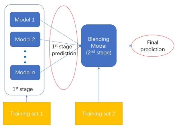
Figure 6: Schematic of the blending method.

In order to have a means of comparison for the combination approach of feature engineering and machine learning algorithms, the raw spectra was processed using state-of-the-art CNN architectures [15]. CNN is well-known for its ability to automatically extract features, thus alleviating the need for feature engineering. The CNN architectures investigated in this research are VGG series [39], Resnet series [22], Inception series [40, 41], Squeeze net [42] and Shuffle net [23].

As these CNNs were originally designed for image classification tasks, some modifications were made prior to using them for the regression task of measuring spatially resolved temperatures. The main changes were as follows: (1) batch normalization and dropout were removed from the networks, as batch normalization shifts the center and standard deviation of the normalization operation with respect to the varied sampling of data, thus leads to high bias and variance for the regression task, (2) the last 399 spectral intensities were discarded, and the remaining 6400 intensities were reshaped to a square image of 80*80. The architectures utilized and modified are from the open-sourced repository: Pytorch-Cifar100 https://github.com/weiaicunzai/pytorch-cifar100.

3 Results and Discussion

3.1 Application of feature engineering and machine learning

3.1.1 Feature engineering

First, we report the application of feature engineering and machine learning methods. The sequence of processing for feature engineering was as follows: (i) physics-guided transformation, (ii) statistical/representation-based feature extraction, (iii) PCA.

After the physics-guided (logarithmicic) transformation, thirty-eight statistical features were extracted from the entire spectrum, which were used as the first group of features. Moreover, for each of the three characteristic bands of H₂O, CO and CO₂, a further thirty-eight features were extracted, respectively, which were then used as the second group of features. The hypothesis, which we wished to explore is whether the information contained within these two sets of features is distinct and complementary. Thus to obtain a comprehensive description of the information of the entire spectrum, the two feature groups were merged together, resulting to a third feature group.

In the case of representation-based features, each spectrum signal was divided into windows of either 20 or 50 spectral samples, followed by their approximation using the four sets of basis functions. The approximation coefficients were then used to represent the information of the spectrum. By doing so, twelve groups of signal representation features were obtained, as shown in Table 3. The notation used for the reporting of the signal representation features involves their order and window length, e.g., 3^rd-20 means third order approximation was used to fit the window data, containing 20 samples.

Table 3: Comparison of fitting quality of Signal representation features

Fitting basis function		Feature number	MSE	R
Polynomial fitting	3rd-20	1356	1.00E-05	1
	3rd-50	540	9.20E-05	0.9999
	2nd-20	1107	3.80E-05	1
	2nd-50	405	0.0003	0.9997
	1st-20	678	0.0001	0.9999
	1st -50	270	0.0011	0.999
Sinusoidal fitting	20	1356	0.3745	0.7623
	50	540	0.0002	0.9997
Exponential fitting	20	1356	-	-
	50	540	-	-
Power fitting	20	1017	9.50E-05	0.9999
	50	405	0.0005	0.9995

In Table 3, we compared the quality of approximation of the various basis functions by using the Mean Square Error (MSE) and Pearson’s correlation coefficient between the original physics-transformed spectra and their reconstructions using signal representation features. In general, the majority of methods offer high quality approximation, as demonstrated in the Tableand Figure 7, except for the exponential, and sinusoidal basis with a window length of 20 samples. This is because the exponential basis functions are not able to reconstruct the spectrum as some of the coefficients become excessively large, leading to overflowing of the exponential function. In the case of sinusoidal basis with a window length of 20, the values of $q$ become very large in the case of smaller windows, thus leading to distortion. This is evident when comparing Figure 7(b), where a spike is observed, in the case of a window with length of 20 samples, against Figure 7(c)), when a window of 50 samples is used. Apart from these two exceptions, the observation is that the higher the order of the fit, and the smaller the window length, the higher the quality of approximation. Moreover, the polynomial basis function approximation is the most accurate among all basis function, for the same number of approximation coefficients. For instance, 2^nd order polynomials vs 1^st order power, and 3^rd order polynomials vs 1^st order sinusoidal approximation. When comparing between polynomial approximations, the case of 3^rd -50 has comparable accuracy to the case 2^nd -20, while the former only has about half the number of features of the latter, and is much better than the case of 1^st-20, although the latter has a larger number of features.

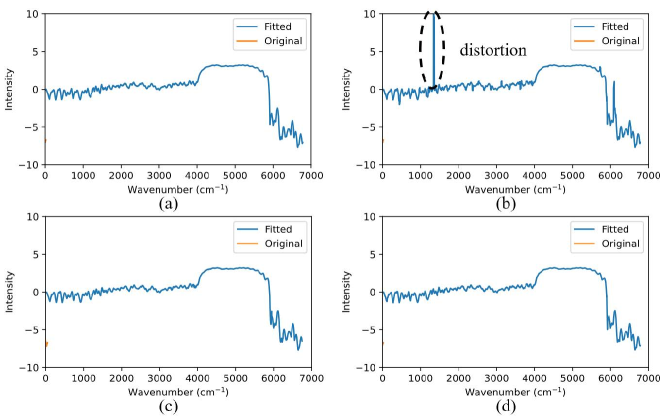
Figure 7: An example of spectrum approximation using: (a) 3^rd order polynomials and a window length of 20; (b) 1^st order sinusoidal basis functions and a window length of 20; (c) 1^st order sinusoidal basis functions and a window length of 50; (d) 1^st order power basis functions and a window length of 20.

Moreover, PCA was applied on all feature groups. Multiple variant feature groups were derived from the original feature group by gradually eliminating the least informative PCA-transformed features. For example, using third-order polynomials and a window size of 50 resulted to 540 features, as the 6799 spectral inputs were divided into 135 windows, each window represented by four features. Following the application of PCA, all 540 PCA-transformed features were considered as a variant feature group, and subsequently reduced in order of decreasing variance to multiples of one hundred, i.e., 500,400,300, etc.

Finally, a wrapper-based feature selection method [43] was used to select the optimal feature groups, where the MLP was used as the referee, and the performance of the feature groups was assessed by its ability in approximating the spatial temperature profiles. The temperature values were normalized in the range of (0,1) using the boundary values in each segment. In principle, this operation can improve the quality of learning. The spectra dataset was divided into training, validation, and test datasets with ratios of 70%, 15% and 15%, respectively. The optimal performances achieved by the various feature groups are summarized in Table 4. The Tableprovides information regarding the size of the original feature vector, the optimal feature vector size following the application of PCA, the optimal number of neurons in the hidden layer of the MLP, and the Mean Square Error (MSE) of training and validation sets on the normalized temperature profiles.

Table 4: Comparison of feature extraction methods

Feature Category	Detailed feature description		Raw Features	PCA Features	Hidden Neurons	Train MSE	Validation MSE
Statistical Features	Entire band		38	38	55	0.042	0.043
	Characteristic bands		114	100	40	0.027	0.028
	Feature aggregation		152	140	50	0.025	0.026
Signal representation features	Polynomial basis	3rd-20	1356	800	15	0.011	0.013
		3rd-50	540	500	20	0.011	0.013
		2nd-20	1107	700	20	0.010	0.013
		2nd-50	405	405	20	0.012	0.014
		1st-20	678	678	20	0.010	0.013
		1st -50	270	200	25	0.015	0.016
	Sinusoidal basis	20	1356	1356	70	0.014	0.017
		50	540	540	25	0.017	0.019
	Exponential basis	20	1356	1356	25	0.013	0.016
		50	540	540	30	0.017	0.019
	Power basis	20	1017	1017	25	0.015	0.016
		50	405	405	25	0.019	0.020

By examining the information in Table 4, we observe that in the case of statistical features, the sets obtained from the characteristic bands perform much better than the set from the whole spectrum range. This is not surprising, since the features extracted from the characteristic bands provide more details. Moreover, the aggregation of statistical features further improves performance, which confirms the hypothesis that the information contained in the two statistical feature groups is distinct and complementary. However, overall, the performance of statistical features is substantially inferior to that of representation-based features. This could be partially due to the number of extracted features; however, a more reasonable explanation is that statistical features are not as powerful as representation-based features in terms of capturing the local shape changes of the emission spectrum. This can be appreciated by observing that the best validation performance acquired by feature aggregation is merely 0.026, while the validation performance acquired by the lowest performing approximation, i.e., polynomial fitting of 1^st-50 is 0.016, which offer an improvement of approximately 38%, with a modest increase of only 60 additional features.

By analyzing the performance of the signal representation-based approach, we observe that polynomial basis approximation provides better results, i.e., a lower training and validation MSE than any other basis functions. For instance, the lowest performing polynomial fit model, i.e., 1^st order with a window of 50 inputs, is comparable with the top performing sinusoidal model, 1^st order with 20 samples, however, it utilizes about one sixth of the number of features. Indeed, the use of higher-order models and smaller window length leads to better performance, since they tend to provide a finer-grained approximation of the spectrum. However, this boosting effect tends to saturate. As shown in the Table, third-order polynomial fitting with a window size of 50 demonstrates negligible performance improvement, compared to those with a window size of 20, although the former results to a smaller number of features. The reason behind this may be that as the spectrum is divided into a larger number of smaller length windows, fitted with polynomial models, there is an increase in redundancy, which is indicated by the comparison in the number of features before and after the application of PCA. By analyzing the performance of the various approximation models, it can be concluded that third-order polynomial fitting with a window size of 50 offers a good compromise between feature complexity and performance.

3.1.2 Machine Learning model performance

Following the feature performance analysis described in the previous section, the group of features obtained through the application of third-order polynomial approximation with a window length of 50 samples was used to train a variety of machine learning models. To reach convergence quickly, all features were normalized to the range of (-1,1), with the outputs (temperatures of segments) normalized in the range of (0, 1). Grid search was performed on the number of features, by varying the amount of features in multiples of one hundred. The temperature values were normalized in the range of (0,1) by using the boundary values in each segment. The performance of the models is summarized in Table 5. In addition to the MSE on the normalized temperature values, the root of the MSE (RMSE), Mean of Relative Error (RE), Relative RMSE (RRMSE) and the Pearson correlation coefficient (R) were assessed on the original temperature values by reversing the estimated normalized temperatures to the original range.

Table 5: Comparison of machine learning models performance

Machine Learning Model	Subclass	Feature number	Normalized Temperature		Original Temperature (test set)
			Train MSE	Test MSE	RMSE (K)	RE	RRMSE	R
MLP	-	500	0.011	0.0129	68.3	0.018	0.027	0.993
RBFN	-	500	0.014	0.0160	75.9	0.020	0.030	0.992
SVR	Linear kernel	540	0.015	0.0161	76.2	0.021	0.030	0.992
	Gaussian kernel	540	0.005	0.0144	72.2	0.019	0.028	0.993
	Polynomial kernel	540	0.006	0.0148	73.1	0.020	0.029	0.992
GPR	Exponential kernel	300	2E-07	0.0165	77.2	0.021	0.030	0.991
	Rational quadratic kernel	500	2E-07	0.0159	75.9	0.021	0.030	0.992
	Matern 32 kernel	200	4E-05	0.0193	83.4	0.023	0.033	0.990
	Matern 52 kernel	200	4E-07	0.0193	83.5	0.024	0.033	0.990
	Square exponential kernel	300	9E-07	0.0224	89.9	0.027	0.035	0.988
Tree-based model	LSBoost	540	0.022	0.0312	106.1	0.031	0.042	0.984
	Random forest	540	0.014	0.0397	119.6	0.037	0.047	0.979
Blending model	Linear Blender	-	0.012	0.0119	65.6	0.017	0.026	0.994
	Heavy Blender	-	0.012	0.0116	64.7	0.017	0.025	0.994
	Light Blender	-	0.012	0.0115	64.3	0.017	0.025	0.994

Training was carried out in two phases. In the first phase, the single-stage models, i.e., MLP, RBF, SVR, GPR and tree-based models were trained and their performance was assessed. The number of hidden neurons in the MLP and RBFN were optimized by grid search. The MLP network was configured to have a single hidden layer, and the hidden neuron number was optimized in the range of (5,100) units, and the optimal value was found to be 20 hidden neurons. In the case of the RBFN, a spread of 1 was selected, with at most 1500 neurons in the hidden layer. The hyperparameters of GPR, SVR, random forest and LSBoost were optimized using Bayes optimization. Early stopping was applied to prevent overfitting. Every model was trained five times to decrease variance, and the models, which performed best on the validation set were selected to be assessed on the test set. Next, attention was turned to the two-stage models, i.e., blending models, in order to further improve the ability to obtain spatially resolved temperature measurements from the spectral profiles.

Among the single-stage models, as shown in Table 5, the MLP performs the best. With the exception of tree-based models, almost all models have comparable performance to that of the MLP, which indicates that the selected features are effective and suiTablefor almost all the algorithms tested in this research.

In order to further improve the prediction performance, the use of model blending was explored. Three variations of the blending model were trained, namely, linear, heavy, and light blender. Their main differences are as follows: (1) Composition of weak learners: Linear blender and heavy blender use all of the single-stage models as weak learners, whereas the light blender model drops tree-based models because of their lower testing performance. (2) Selection of meta learner: Linear blender utilizes ordinary Least Squares (OLS) estimation, while both heavy and light blenders employ a MLP.

As shown in Table 5, using a blending method results to performance improvements. All three blending models perform better than the MLP model with respect to the metrics of Table 5. However, it is also noted that this comes at the expense of increased computational and storage costs, as the blending models require the supports of a large number of weak learners. It is also shown that the MLP is a better meta learner than OLS, since the linear blender delivers a lower performance, which is not surprising, due to its linear nature, unlike the nonlinear processing capabilities of the MLP. Moreover, elimination of the lower performing tree-based models is beneficial, as it results to the light blender achieving the best performance.

Figure 8 displays representative temperature profile estimation examples on the test set, provided by the MLP and the Light Blender model. Both models work well, although their performance slightly degrades, when dealing with gradually irregular profiles, as shown in Figures8 (e)-(f).

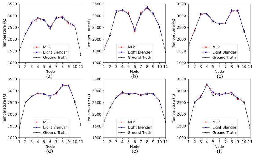
Figure 8: Performance of MLP and Blender light model in recovering non-uniform temperature profiles. (a) Dual-peak Gaussian profile with a relatively small temperature variation;(b) Dual-peak Gaussian profile with a relatively large temperature variation; (c) Irregular dual-peak Gaussian profile with two “flatlands”; (d) Temperature profile with an increasing trend; (e) Trapezoidal temperature profile, (f) Temperature profile with a rush peak

3.2 Application of Convolutional Neural Networks on raw spectra

Eleven CNN models were trained with the raw spectral measurements as input, which includes VGG series, Resnet series, Inceptron series, shuffle net and Squeeze net. Among them, VGG series [39] are the most classical CNN architectures, which uses purely stacked convolutional layers, while ResNet [22] adds the skip connection to achieve the concept of residual learning, Inception [40, 41] uses convolution kernels of varying sizes to sense diverse receptive fields, while Xception, the ultimate evolution of Inceptron, Shuffle net [23] and Squeeze net [42] are light level networks with more modern designs.

In the training, Adam [44] was used as the optimization method, and a weight decay of 1e-4 was used to alleviate overfitting. The learning rate was preliminarily determined by the method suggested in [45], however, it was further decreased as the selected deep learning models were prone to overfitting the training set, particularly, after removing the dropout and normalization operations, required for the regression application. According to such an operation, the learning rate was configured and varied for the various CNN architectures. In order to better navigate the training direction, the warm-up operation  [46] was used to train the networks in the first ten epochs, during which, the learning rate was gradually increased from a tiny value to the selected learning rate. Such a soft activation of training supports the appropriate choice of training direction. During the normal training process, the Cosine Annealing learning rate schedule  [46] was used, which helps to avoid falling into local minima.

The test performances of the CNN models are summarized in Table 6. Overall, all CNN models have similar performance, so that, to some extent, the results can represent the performance level, which can be reached by conventional CNN architectures with raw spectra as inputs. Strictly speaking, the best performance based on the metrics of Table 6 is achieved by Resnet18. However, when compared to the results obtained from the combination of feature engineering and classical machine learning methods, the temperature measurement estimates using CNN are worse than most of classical machine learning models. Specifically, when comparing Tables 5 and  6 , it is apparent that the values of the RMSE, RE and RRMSE metrics for Resnet18 are almost double compared to those of the light blender model.

Table 6: Performance comparison of CNN architectures

CNN Model	Subclass	Normalized Temperature		Original Temperature
		Train MSE	Test MSE	RMSE	RE	RRMSE	R
VGG	VGG11	0.032	0.037	114.3	0.033	0.045	0.981
	VGG13	0.032	0.036	113.7	0.033	0.045	0.981
	VGG16	0.033	0.038	116.9	0.034	0.046	0.980
	VGG19	0.040	0.043	124.1	0.037	0.049	0.978
Resnet	Resnet18	0.026	0.033	108.9	0.031	0.043	0.983
	Resnet34	0.031	0.035	111.0	0.032	0.044	0.982
	Resnet50	0.028	0.033	109.4	0.032	0.043	0.983
Inception	V3	0.033	0.036	113.4	0.033	0.044	0.981
	Xception	0.032	0.035	112.9	0.033	0.044	0.982
Shuffle net	-	0.032	0.036	113.4	0.033	0.044	0.981
Squeeze net	-	0.034	0.039	119.2	0.035	0.047	0.979

A more direct comparison between Resnet18 and the light blender is provided in Figure 9. Although Resnet18 can satisfactorily capture the basic features of the morphology of temperature profiles, it cannot provide as accurate temperature estimations as the light blender model. This comparison indicates that effective feature engineering, which is often replaced by the built-in feature extraction of CNN in the state-of-the-art  [47, 48, 49], can enable classical machine learning algorithms to achieve competitive performance.

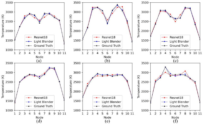
Figure 9: Comparison between Resnet18 and the light blender models. (a) Dual-peak Gaussian profile with a relatively small temperature variation;(b) Dual-peak Gaussian profile with a relatively large temperature variation; (c) Irregular dual-peak Gaussian profile with two “flatlands”; (d) Temperature profile with an increasing trend; (e) Trapezoidal temperature profile, (f) Temperature profile with a rush peak.

3.3 Comparison with state-of-the-art

The methods described in [12, 13] were applied to the dataset used in this study. To the best of the authors’ knowledge, these are the only two studies where data-driven models are used to measure spatially resolved temperature profiles from emission spectroscopy. Both methods employ the MLP model. In [12], the conventional single hidden layer architecture is employed, whereas in [13], three hidden layers are used. In this work, the MLP architectures of these studies were precisely replicated. We performed grid search to fine-tune the hyperparameters of the associated MLP models. In terms of feature engineering, no feature engineering is used in [13], rather, the raw spectra data is directly fed to the MLP. In [12], the spectrum is divided into windows of fixed length, and the ratios of line intensities at the two sides of the spectrum are used as features. Two window lengths of 10 and 20 samples were explored in this work.

In summary, three MLP models, two with the setup of [12], and one with the architecture of [13], were developed and trained. As demonstrated in Table 7, the light blender model (see Table 5) offers significant performance improvements, compared to these three models. A visual comparison of the performance of the two methods compared to the light blender model is given in Figure 10, where it can be observed that, in general, the methods of [12] and [13] capture the properties of the dual-peak Gaussian profiles, which constitute the majority of the training set, but have very limited adaptability to irregular profiles, although the method in [12] is slightly better.

Table 7: Performance of the state-of-the-art methods

Method	Model	Input	RMSE	RE	RRMSE	R
[13]	MLP (Three hidden layers)	Raw spectrum	165.7	0.055	0.065	0.96
[12]	MLP	Intensity ratios, window length of 50 samples)	130.5	0.04	0.051	0.975
	MLP	Intensity ratios, window length of 20 samples	130	0.04	0.051	0.976

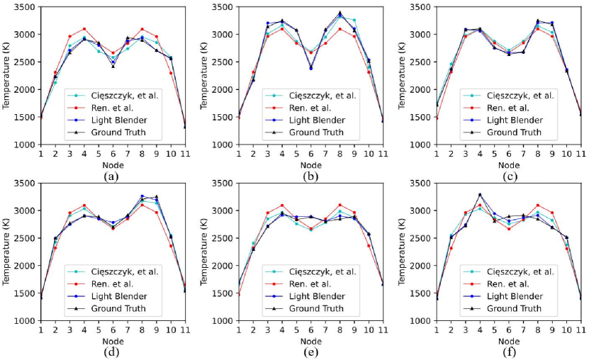
Figure 10: Comparation between the state-of-the-art approaches of [12, 13] and the light blender model. (a) Dual-peak Gaussian profile with a relatively small temperature variation;(b) Dual-peak Gaussian profile with a relatively large temperature variation; (c) Irregular dual-peak Gaussian profile with two “flatlands”; (d) Temperature profile with an increasing trend; (e) Trapezoidal temperature profile, (f) Temperature profile with a rush peak.

It is also notable that the CNNs (see Table 6), which were tested in this work, offer better performance than the two state-of-the-art methods. This supports the use of CNNs with their powerful capabilities in approximating complex mappings, compared to traditional MLP models. In turn, this highlights the importance of effective feature engineering, which when combined with machine learning models, such as the one-stage MLP, can deliver better performance than CNNs.

4 Conclusions

In this work, we systematically explored the feasibility of using data-driven models to recover spatially resolved temperature distributions from line-of-sight emission spectroscopy data. Two types of data-driven models were considered: (a) coupling of feature engineering and classical machine learning methods, and (b) end-to-end Convolutional Neural Networks. The main conclusions which can be drawn are as follows:

1. The combination of physics-guided transformation, polynomial approximation-based features, and PCA is the most effective feature extraction methodology among the feature engineering methods attempted in this research.

2. When using the selected group of features, the light blender model, an non-linear ensemble learning model, offers the best performance among fifteen traditional machine learning models, with RMSE, RE, RRMSE and R values of 64.3, 0.017, 0.025 and 0.994, respectively. This demonstrates the feasibility and capability of data-driven models in measuring nonuniform spatial temperature distributions from emission spectroscopy data.

3. State-of-the-art Convolutional Neural Networks offer competitive performance compared to state-of-the-art techniques, however, they are not able to match the performance of feature engineering and machine learning models. This supports the effectiveness of feature engineering in providing substantial advantages in the context of estimating spatially resolved temperature distributions from line-of-sight spectroscopy data.

As for further work, it is considerable that generating more diverse temperature profile datasets, so as to further expand the application scenarios and assess the limitations of the proposed method. Moreover, we will consider further opportunities for feature engineering of emission spectroscopy data to determine more effective feature sets in order to improve the accuracy of the proposed framework.

References

- [1] Susan Meerdink, Dar Roberts, Glynn Hulley, Paul Gader, Jan Pisek, Kairi Adamson, Jennifer King, and Simon J. Hook. Plant species’ spectral emissivity and temperature using the hyperspectral thermal emission spectrometer (HyTES) sensor. Remote Sensing of Environment, 224:421–435, April 2019.
- [2] Peter R. Solomon, Philip E. Best, Robert M. Carangelo, James R. Markham, Po-Liang Chien, Robert J. Santoro, and Hratch G. Semerjian. FT-IR emission/transmission spectroscopy for in situ combustion diagnostics. Symposium (International) on Combustion, 21(1):1763–1771, January 1988.
- [3] Thangam Parameswaran, Robin Hughes, Peter Gogolek, and Patrick Hughes. Gasification temperature measurement with flame emission spectroscopy. Fuel, 134:579–587, October 2014.
- [4] Guannan Liu and Dong Liu. Inverse radiation problem of multi-nanoparticles temperature and concentration fields reconstruction in nanofluid fuel flame. Optik, 181(December 2018):81–91, 2019.
- [5] S. Einecke, C. Schulz, and V. Sick. Measurement of temperature, fuel concentration and equivalence ratio fields using tracer LIF in IC engine combustion. Applied Physics B, 71(5):717–723, November 2000.
- [6] Max Gerhards, Martin Schlerf, Kaniska Mallick, and Thomas Udelhoven. Challenges and Future Perspectives of Multi-/Hyperspectral Thermal Infrared Remote Sensing for Crop Water-Stress Detection: A Review. Remote Sensing, 11(10):1240, May 2019.
- [7] Sander Veraverbeke, Philip Dennison, Ioannis Gitas, Glynn Hulley, Olga Kalashnikova, Thomas Katagis, Le Kuai, Ran Meng, Dar Roberts, and Natasha Stavros. Hyperspectral remote sensing of fire: State-of-the-art and future perspectives. Remote Sensing of Environment, 216:105–121, October 2018.
- [8] Roman V. Kochanov, I. E. Gordon, L. S. Rothman, P. Wcisło, C. Hill, and J. S. Wilzewski. HITRAN Application Programming Interface (HAPI): A comprehensive approach to working with spectroscopic data. Journal of Quantitative Spectroscopy and Radiative Transfer, 177:15–30, 2016.
- [9] Hyun Keol Kim and Tae Ho Song. Determination of the gas temperature profile in a large-scale furnace using a fast/efficient inversion scheme for the SRS technique. Journal of Quantitative Spectroscopy and Radiative Transfer, 93(1-3 SPEC. ISS.):369–381, 2005.
- [10] Tae Ho Song. Spectral remote sensing for furnaces and flames. Heat Transfer Engineering, 29(4):417–428, 2008.
- [11] Tao Ren and Michael F. Modest. Temperature profile inversion from co2 spectral intensities through levenberg-marquardt optimization and tikhonov regularization. AIAA AVIATION 2014 -11th AIAA/ASME Joint Thermophysics and Heat Transfer Conference, (June):1–9, 2014.
- [12] S. Cięszczyk. Determination of plume temperature distribution based on the ratios of the radiation intensities of multiple CO 2 lines. Optical Sensors 2015, 9506(2):950623–950623, 2015.
- [13] Tao Ren, Michael F. Modest, Alexander Fateev, Gavin Sutton, Weijie Zhao, and Florin Rusu. Machine learning applied to retrieval of temperature and concentration distributions from infrared emission measurements. Applied Energy, 252(May):113448–113448, 2019.
- [14] M.W Gardner and S.R Dorling. Artificial neural networks (the multilayer perceptron)—a review of applications in the atmospheric sciences. Atmospheric Environment, 32(14-15):2627–2636, August 1998.
- [15] Ahmed Ali Mohammed Al-Saffar, Hai Tao, and Mohammed Ahmed Talab. Review of deep convolution neural network in image classification. In 2017 International Conference on Radar, Antenna, Microwave, Electronics, and Telecommunications (ICRAMET), pages 26–31, Jakarta, October 2017. IEEE.
- [16] Po-Lung Chen, Chen-Tse Tsai, Yao-Nan Chen, Ku-Chun Chou, Chun-Liang Li, Cheng-Hao Tsai, Kuan-Wei Wu, Yu-Cheng Chou, Chung-Yi Li, Wei-Shih Lin, et al. A linear ensemble of individual and blended models for music rating prediction. In Proceedings of KDD Cup 2011, pages 21–60. PMLR, 2012.
- [17] G. V. Trunk. A Problem of Dimensionality: A Simple Example. IEEE Transactions on Pattern Analysis and Machine Intelligence, PAMI-1(3):306–307, July 1979.
- [18] Zainab Husain, Nadya Abdel Madjid, and Panos Liatsis. Tactile Sensing Using Machine Learning-Driven Electrical Impedance Tomography. IEEE Sensors Journal, 21(10):11628–11642, May 2021.
- [19] Hervé Abdi and Lynne J. Williams. Principal component analysis. Wiley Interdisciplinary Reviews: Computational Statistics, 2(4):433–459, July 2010.
- [20] S. Elanayar V.T. and Y.C. Shin. Radial basis function neural network for approximation and estimation of nonlinear stochastic dynamic systems. IEEE Transactions on Neural Networks, 5(4):594–603, July 1994.
- [21] Christopher K Williams and Carl Edward Rasmussen. Gaussian Processes for Machine Learning, volume 2. MIT press Cambridge, MA, 2006.
- [22] Kaiming He, Xiangyu Zhang, Shaoqing Ren, and Jian Sun. Deep residual learning for image recognition. In Proceedings of the IEEE Conference on Computer Vision and Pattern Recognition, pages 770–778, 2016.
- [23] Xiangyu Zhang, Xinyu Zhou, Mengxiao Lin, and Jian Sun. ShuffleNet: An Extremely Efficient Convolutional Neural Network for Mobile Devices, December 2017.
- [24] L.S. Rothman, I.E. Gordon, R.J. Barber, H. Dothe, R.R. Gamache, A. Goldman, V.I. Perevalov, S.A. Tashkun, and J. Tennyson. HITEMP, the high-temperature molecular spectroscopic database. Journal of Quantitative Spectroscopy and Radiative Transfer, 111(15):2139–2150, October 2010.
- [25] Ronald K. Hanson, R. Mitchell Spearrin, and Christopher S. Goldenstein. Spectroscopy and Optical Diagnostics for Gases. Springer International Publishing, Cham, 2016.
- [26] T. L. Bergman and Frank P. Incropera, editors. Fundamentals of Heat and Mass Transfer. Wiley, Hoboken, NJ, 7th ed edition, 2011.
- [27] Gamal Daniel Roston and F. S. Obaid. Exact analytical formula for Voigt spectral line profile. Journal of Quantitative Spectroscopy and Radiative Transfer, 94(2):255–263, 2005.
- [28] C. S. Goldenstein, I. A. Schultz, R. M. Spearrin, J. B. Jeffries, and R. K. Hanson. Scanned-wavelength-modulation spectroscopy near 2.5 m for H 2O and temperature in a hydrocarbon-fueled scramjet combustor. Applied Physics B: Lasers and Optics, 116(3):717–727, 2014.
- [29] Xiang Liu, Jay B. Jeffries, and Ronald K. Hanson. Measurement of nonuniform temperature distributions using line-of-sight absorption spectroscopy. AIAA Journal, 45(2):411–419, 2007.
- [30] Leyen S. Chang, Christopher L. Strand, Jay B. Jeffries, Ronald K. Hanson, Glenn S. Diskin, Richard L. Gaffney, and Diego P. Capriotti. Supersonic mass-flux measurements via tunable diode laser absorption and nonuniform flow modeling. AIAA Journal, 49(12):2783–2791, 2011.
- [31] Oliver N. Keene. The log transformation is special. Statistics in Medicine, 14(8):811–819, April 1995.
- [32] S. Golgiyaz, Muhammed Fatih Talu, and Cem Onat. Artificial neural network regression model to predict flue gas temperature and emissions with the spectral norm of flame image. Fuel, 255(April):115827–115827, 2019.
- [33] Yngve Ögren, Pál Tóth, Attila Garami, Alexey Sepman, and Henrik Wiinikka. Development of a vision-based soft sensor for estimating equivalence ratio and major species concentration in entrained flow biomass gasification reactors. Applied Energy, 226(May):450–460, 2018.
- [34] William S Noble. What is a support vector machine? Nature Biotechnology, 24(12):1565–1567, December 2006.
- [35] Omer Sagi and Lior Rokach. Ensemble learning: A survey. WIREs Data Mining and Knowledge Discovery, 8(4), July 2018.
- [36] Daniel Borup, Bent Jesper Christensen, Nicolaj Søndergaard Mühlbach, and Mikkel Slot Nielsen. Targeting predictors in random forest regression. International Journal of Forecasting, page S0169207022000395, April 2022.
- [37] Tianqi Chen and Carlos Guestrin. Xgboost: A scalable tree boosting system. In Proceedings of the 22nd Acm Sigkdd International Conference on Knowledge Discovery and Data Mining, pages 785–794, 2016.
- [38] Ravi K. Samala, Heang-Ping Chan, Lubomir Hadjiiski, and Sathvik Koneru. Hazards of data leakage in machine learning: A study on classification of breast cancer using deep neural networks. In Horst K. Hahn and Maciej A. Mazurowski, editors, Medical Imaging 2020: Computer-Aided Diagnosis, page 39, Houston, United States, March 2020. SPIE.
- [39] Karen Simonyan and Andrew Zisserman. Very Deep Convolutional Networks for Large-Scale Image Recognition, April 2015.
- [40] François Chollet. Xception: Deep Learning with Depthwise Separable Convolutions, April 2017.
- [41] Christian Szegedy, Wei Liu, Yangqing Jia, Pierre Sermanet, Scott Reed, Dragomir Anguelov, Dumitru Erhan, Vincent Vanhoucke, and Andrew Rabinovich. Going Deeper with Convolutions, September 2014.
- [42] Forrest N. Iandola, Song Han, Matthew W. Moskewicz, Khalid Ashraf, William J. Dally, and Kurt Keutzer. SqueezeNet: AlexNet-level accuracy with 50x fewer parameters and 0.5MB model size, November 2016.
- [43] Naoual El Aboudi and Laila Benhlima. Review on wrapper feature selection approaches. In 2016 International Conference on Engineering & MIS (ICEMIS), pages 1–5, Agadir, Morocco, September 2016. IEEE.
- [44] Diederik P. Kingma and Jimmy Ba. Adam: A Method for Stochastic Optimization, January 2017.
- [45] Leslie N. Smith. Cyclical Learning Rates for Training Neural Networks, April 2017.
- [46] Akhilesh Gotmare, Nitish Shirish Keskar, Caiming Xiong, and Richard Socher. A Closer Look at Deep Learning Heuristics: Learning rate restarts, Warmup and Distillation. arXiv:1810.13243 [cs, stat], October 2018.
- [47] Daniel Weimer, Bernd Scholz-Reiter, and Moshe Shpitalni. Design of deep convolutional neural network architectures for automated feature extraction in industrial inspection. CIRP Annals, 65(1):417–420, 2016.
- [48] Yao Liu, Hongbin Pu, and Da-Wen Sun. Efficient extraction of deep image features using convolutional neural network (CNN) for applications in detecting and analysing complex food matrices. Trends in Food Science & Technology, 113:193–204, July 2021.
- [49] Thomas Wiatowski and Helmut Bolcskei. A Mathematical Theory of Deep Convolutional Neural Networks for Feature Extraction. IEEE Transactions on Information Theory, 64(3):1845–1866, March 2018.