Unsupervised Object Localization:
Observing the Background to Discover Objects

Abstract

Recent advances in self-supervised visual representation learning have paved the way for unsupervised methods tackling tasks such as object discovery and instance segmentation. However, discovering objects in an image with no supervision is a very hard task; what are the desired objects, when to separate them into parts, how many are there, and of what classes? The answers to these questions depend on the tasks and datasets of evaluation. In this work, we take a different approach and propose to look for the background instead. This way, the salient objects emerge as a by-product without any strong assumption on what an object should be. We propose FOUND, a simple model made of a single $conv1\times 1$ initialized with coarse background masks extracted from self-supervised patch-based representations. After fast training and refining these seed masks, the model reaches state-of-the-art results on unsupervised saliency detection and object discovery benchmarks. Moreover, we show that our approach yields good results in the unsupervised semantic segmentation retrieval task. The code to reproduce our results is available at https://github.com/valeoai/FOUND.

Figure 1: Examples of object localization results obtained with our method FOUND on images from diverse datasets. We propose a simple framework in which we train a single $conv1\times 1$ layer, and achieve state-of-the-art results in unsupervised object discovery and saliency detection. We train for only 2 epochs over the 10k dataset DUTS-TR [55] and inference runs at $80$ FPS. Note that the results presented here are without post-processing refinement.

1 Introduction

The task of object localization — either performed by detecting [40, 4] or segmenting [7] objects — is required in many safety-critical systems such as self-driving cars. Today’s best methods train large deep models [4, 7] on large sets of labeled data [30, 13]. To mitigate such needs in annotation, it is possible to use strategies such as semi-supervised [32, 10], weakly-supervised [62, 10] and active learning [66, 38, 51].

In this work, we consider the unsupervised object localization task, which consists in discovering objects in an image with no human-made annotation. This task has recently received a lot of attention [42, 44, 41] as it is a solution to detect objects in a scene with no prior about what they should look like or which category they should belong to. Early works exploit hand-crafted features [63, 73, 47, 76] and inter-image information [50, 52] but hardly scale to large datasets. Recent works leverage strong self-supervised [16, 6, 19] features learned using pretext tasks: [45, 59, 34] localize a single object per image just by exploiting a similarity graph at the level of an image; [44] proposes to combine different self-supervised representations, in an ensemble-fashion, and trains a model to learn the concept of object, the same as what [57] does. However, most of these methods make assumptions about what an object is. For example, [45, 59] assume that an image contains more background pixels than object pixels, while [44] discards masks that fill in the width of an image. Such hypotheses restrict objects one can find.

In this work, we propose to tackle the problem the other way around: we make no assumptions about objects but focus instead on the concept of background. Then, we use the idea that a pixel not belonging to the background is likely to belong to an object. Doing so, we do not need to make hypotheses about the number or the size of objects in order to find them. Our method, named FOUND, is cheap both at training and inference time.

We start by computing a rough estimate of the background mask; this step works by mining a first patch that likely belongs to the background. To do this, we leverage attention maps in a self-supervised transformer and select one of the patches that received the least attention. Then the background mask incorporates patches similar to this mined one. One of our contributions is a reweighting scheme to reduce the effect of noisy attention maps based on the sparsity concept. In the second step, we use the fact that the complement of this background mask provides an approximate estimation of the localization of the objects. This estimate is refined by training a single $conv1\times 1$ layer on top of the frozen self-supervised transformer, using only the masks computed in the first step, an edge-preserving filter, and a self-labelling procedure. We show that this cheap method allows us to reach state-of-the-art results in the tasks of saliency detection, unsupervised object discovery and semantic segmentation retrieval.

Our main contributions are as follows:

• We propose to think about the object discovery problem upside-down, and to look for what is not background instead of directly looking for objects.

• We propose a new way to exploit already self-trained features and show that they allow us to discover the concept of background.

• We show that the use of attention heads can be improved by integrating a weighting scheme based on attention sparsity.

• We propose a lightweight model composed only of a single $conv1\times 1$ layer and show that there is no need to train a large segmenter for the task.

• We demonstrate that our model performs well on unsupervised saliency detection, unsupervised object discovery and unsupervised semantic segmentation retrieval tasks. We reach state-of-the-art results in all tasks with a method much faster and lighter than competing ones.

2 Related work

Self-supervised learning.

In self-supervised learning, a model is trained to solve a pretext task (e.g., jigsaw solving, colorization, or rotation prediction) on unlabeled data [37, 27, 17, 6, 16, 8, 46, 20, 9]. Recently, with the surge of Vision Transformers (ViT) [12] that stand out compared to convolutional networks, one can obtain rich, and dense descriptors of image patches with models trained in a self-supervised fashion on massive amounts of data [6, 19, 72]. For example, DINO [6] employs a teacher-student framework where the two networks see different and randomly transformed input parts and the student network learns to predict the mean-centered output of the teacher network. In MAE [19], patches of the input image are randomly masked and the pretext task aims at learning to reconstruct the missing pixels by auto-encoding. In these works, it has been shown that the representations of the self-attention maps of the ViTs contain interesting localization information [6, 19, 72, 1], which have led recent methods to exploit these properties in several downstream tasks as unsupervised object discovery [45, 59, 34] or semantic segmentation [18, 67, 15, 48]. In this paper, we build upon such self-supervised features to partition background and foreground patches. Arguably, learning self-supervised representation on unlabaled Imagenet [11] — a curated dataset — induces a certain supervision. We leave for future work using models trained on less curated and more heterogenous datasets.

Unsupervised object localization.

Localizing objects within images without any supervision is in the literature traditionally addressed by two distinct branches: 1) unsupervised saliency detection methods find binary masks of objects [64, 74, 29] while 2) unsupervised object detection seeks for bounding boxes around objects [26, 23, 3, 75]. Unsupervised saliency detection has been approached with hand-crafted methods [63, 73], generative adversarial models [35], or, closer to us, by refining noisy labels [36]. The first attempts in an unsupervised object discovery have often used region proposals [76, 47] as input. These works explored a collection of images and inter-image information using methods such as principal component analysis [60], optimization [49, 50] or ranking [53].

Recently, these historically distinct tasks have been tackled jointly in unified frameworks [59, 34, 39] building on the advent of aforementioned self-trained dense visual features [9, 5, 6, 19]. Given an image, these methods create a weighted graph where each node is a patch, and edges represent the similarity between the patches. Foreground objects are segmented by leveraging this similarity. In particular, LOST [45] uses this graph to mine an object seed as the patch with the least connection to other patches and expands the zone of interest to all connected similar patches afterwards. Building on LOST, TokenCut [59] and Deep Spectral Methods [34] refine this result by using a normalized graph-cut to separate an object from the highly connected patches, which most likely depict the background.

Another line of methods proposes to compute mask proposals that are later refined. SelfMask [44] explores the use of multiple self-supervised features [9, 5, 6] as the input of a spectral clustering algorithm. FreeSOLO [57] proposes FreeMask that generates correlation maps which are then ranked and filtered by a maskness score. DINOSAUR [42] performs representation learning by separating the features of an image and reconstructing them into individual objects or parts.

It should be noted that these prior works make strong underlying assumptions about what an object is. This includes priors about the contrast [22], the size [45, 59], the centerness [24], the shape [44] or boundary [61] of the sought object. Instead, in our work, by looking for the background, we do not need to make any assumptions about the presence or number of objects.

Learning to generalize through training.

While we build our seed masks from single-image information, we refine these masks in a self-training step that leverages information shared across the whole image collection. This self-training step aims at improving the quality of predictions by propagating and refining the initial seed of pseudo-annotations to a large set of unlabeled instances. Early works in unsupervised saliency detection learn a deep unsupervised saliency network from noisy predictions obtained from handcrafted methods [68, 69, 36]. After clustering self-supervised features, [45, 59] train a Class-Agnostic Detection (CAD) network over predicted pseudo-boxes and show that this trained detector can smooth out poor discoveries, therefore boosting results. Similarly, in semantic segmentation, FreeSOLO [57] and COMUS [67] feed coarse masks to train a segmentation model on these pseudo masks [56].

When propagating and refining pseudo-labels through the dataset with training, previous methods generally employ heavy training procedures involving learning several millions of parameters. Instead, our self-training step is extremely lightweight and fast as it is only composed of one layer of 1$\times$1 convolutions and a two-epoch training scheme.

3 Our method FOUND

In this work, we tackle the unsupervised object localization task by considering the problem upside-down. Our approach consists of two stages. First, we propose to look for patches corresponding to the background in order to highlight patches that are likely objects (Sec. 3.1). Then, starting from these coarse masks, we design a fast and lightweight self-supervised learning scheme to refine them (Sec. 3.2). An overview of FOUND is shown in Fig. 2.

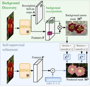
Figure 2: Overview of FOUND. In the first stage (green upper part), a background mask $\mathbf{M^{b}}$ is discovered by mining a seed patch through a reweighting of the self-attention maps of a frozen DINO [6]. This seed is then used to find similar patches likely belonging to the background. In the second stage (blue lower part), we train a lightweight $1\times 1$ convolutional layer that produces refined masks from DINO features. It is trained in a self-supervised fashion to predict both smoothed inverse coarse masks $\mathbf{M^{b}}$ of the first step, and smoothed binarized version of its own output. Blue arrows denote where the gradients flow (in the reverse direction).

3.1 Background discovery

Here, we look for the background pixels of an image $\mathbf{I}\in\mathbb{R}^{W\times H\times 3}$. To do so, we start by extracting deep features from this image using a self-supervised pre-trained ViT. First, the image is divided into $N$ square patches of $P$ pixels each. These patch tokens, along with an additional learned token, called class token (CLS), are processed by the ViT. At the last self-attention layer, composed of $h$ different heads, we extract $h$ matrices $\{\mathbf{F}_{i}\in\mathbb{R}^{N\times d}\}_{i=1..h}$, that each contains $d$-dimensional features for each of the $N$ patches. We also store in $\mathbf{A}\in\mathbb{R}^{N\times h}$ the $h$ self-attention maps between the CLS token and all patch tokens.

Background seed.

To identify the background, we start by identifying one patch which likely belongs to the background. This patch, called the background seed, is defined as the patch with the least attention in $\mathbf{A}$ — a patch which the model has learned to not give too much attention to. This seed is the $s^{\rm th}$ patch, where

$$s=\operatorname*{argmin}_{p\ \in\ \{1,\ldots,N\}}\sum_{i=1}^{h}\mathbf{A}_{pi}.$$ (1)

In the equation above, $\mathbf{A}_{pi}$ is the attention score between the CLS token and the $p^{\rm th}$ patch in the $i^{\rm th}$ attention head.

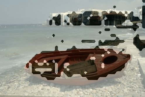
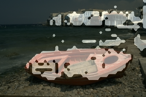
(a) Coarse background mask $\mathbf{M}^{b}$	(b) Coarse foreground mask $\mathbf{M}^{f}$
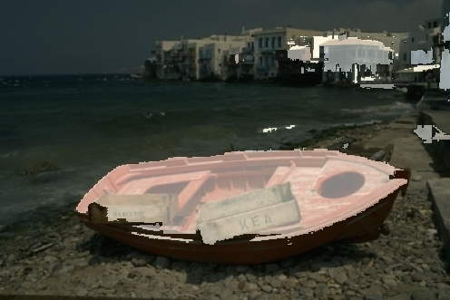
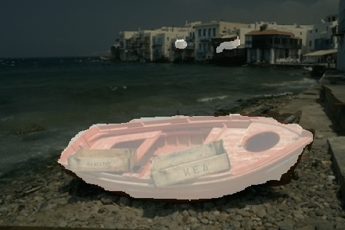
(c) Refined $\zeta(\mathbf{M}^{f})$	(d) Predicted $\mathbf{M}^{s}$

Figure 3: Visualizations of masks generated for one image from ECSSD [43] at different stages of our method. We show (a) the mask $\mathbf{M}^{b}$ extracted using our background discovery step, (b) its inverse $\mathbf{M}^{f}$ used as foreground mask to train our segmenter head, (c) the version refined using a bilateral solver $\zeta(\mathbf{M}^{f})$ and (d) the output of our segmentation head $\mathbf{M}^{s}$ at the end of the training.

Reweighting the attention heads.

When observing the $h$ different attention maps in $\mathbf{A}$, we notice that the background appears more or less clearly in the different heads. Therefore, we propose to weight each head differently in Eq. 1. We exploit the sparsity of the attention map to compute these weights since the background appears better in a sparse attention map (as illustrated in the supplementary materials). Inspired by [25], we compute the sparsity $S_{i}$ of each map by counting the number of attention values above a certain threshold $\mu>0$:

$$S_{i}=|\{p\ |\ A_{pi}\geq\mu,\;p=1,\ldots,N\}|,$$ (2)

and reweight each attention map in (1) by

$$w_{i}=\log\left(\frac{\sum_{j=1}^{h}S_{j}}{S_{i}}\right).$$ (3)

Notice that $w_{i}$ increases when the sparsity $S_{i}$ decreases, i.e., when we visually observe a clearer separation of the background from the foreground thanks to sparser attention maps. Finally, Eq. 1 becomes

$$s=\operatorname*{argmin}_{p\ \in\ \{1,\ldots,N\}}\sum_{i=1}^{h}w_{i}\,\mathbf{A}_{pi}.$$ (4)

Discovery of the background.

We identify the background by finding patches similar to the background seed. For each patch, we start by computing a single feature by concatenating the corresponding $d$-dimensional features in each head: ${\tilde{\mathbf{F}}=[w_{1}\,\mathbf{F}_{1},\ldots,w_{h}\,\mathbf{F}_{h}]\in\mathbb{R}^{N\times hd}}$. Then, the background mask $\mathbf{M}^{b}\in\{0,1\}^{N}$ is defined as

$$\mathbf{M}^{b}_{p}=\begin{cases}1&\text{if }{\rm sim}(\tilde{f}_{p},\tilde{f}_{s})\geq\tau,\\ 0&\text{otherwise},\end{cases}\;p=1,\ldots,N,$$ (5)

for a threshold $\tau>0$, where ${\rm sim}$ is the cosine similarity, and $\tilde{f}_{p}$, $\tilde{f}_{s}$ are the $hd$-dimensional features corresponding to patch $p$ and $s$ in $\tilde{\mathbf{F}}$. We show an example in Fig. 3.

3.2 Refining masks with self-training

The proposed background discovery method described above is able to segment a good portion of the background but the corresponding masks are still far from perfect, as observed in Fig. 3. To improve them, and therefore to better segment the foreground objects, we propose a very simple refinement step of learning a lightweight segmentation head in a self-supervised fashion.

The segmentation head consists of a single $1\times 1$ convolution. For each patch, it compresses DINO frozen patch features into a scalar, which is passed into a sigmoid function to encode the probability of the patch belonging to the foreground. We stress that, unlike most recent works, we do not train a heavy segmentation backbone [67, 44, 57] or a detection model [45, 59]. This aspect brings considerable training and inference efficiency both in terms of time and memory, as studied in Sec. 4.4.

The segmentation head is trained in a self-supervised fashion. The general idea is that the model learns to predict a smoothed version of the complement of the coarse background masks and its own prediction, such that it quickly converges to refined masks. We describe it formally below.

Segmentation head training.

Self-training is done thanks to two losses with distinct roles. The first objective consists of initializing and guiding the predictions toward the coarse background masks. The second objective aims at smoothing and refining predictions.

Formally, let $\mathbf{M}^{s}\in\mathbb{R}^{N}$ be the soft output of the segmentation head for a given image. The goal of the first objective is to predict the complement $\mathbf{M}^{f}$ of the coarse background mask $\mathbf{M}^{b}$ (defined in Sec. 3.1), refined by a bilateral solver $\zeta(\cdot)$, which is an edge-aware smoothing technique improving the mask quality as proposed in [2] and exploited in [59, 44]. Let $\hat{\mathbf{M}}^{f}\in\{0,1\}^{N}$ be this refined version. We compute the binary cross entropy

$$\mathcal{L}^{f}=\sum_{p=1}^{N}\left[\hat{\mathbf{M}}^{f}_{p}\log\mathbf{M}^{s}_{p}+(1-\hat{\mathbf{M}}^{f}_{p})\log(1-\mathbf{M}^{s}_{p})\right]$$ (6)

over a batch of images, where $\mathbf{M}^{s}_{p}$ and $\hat{\mathbf{M}}^{f}_{p}$ are the output of the segmentation head and refined coarse mask at patch $p$ respectively. We additionally train the segmentation head by minimizing the binary cross entropy between the output and its refined version after binarization $\hat{\mathbf{M}}^{s}\in\mathbb{R}^{N}$, using again the bilateral solver, in order to force the quality of the mask edges, using

$$\mathcal{L}^{s}=\sum_{p=1}^{N}\left[\hat{\mathbf{M}}^{s}_{p}\log\mathbf{M}^{s}_{p}+(1-\hat{\mathbf{M}}^{s}_{p})\log(1-\mathbf{M}^{s}_{p})\right]$$ (7)

with $\hat{\mathbf{M}}^{s}_{p}$ being the refined mask at patch $p$. Note that we compute this loss only for images for which $\mathbf{M}^{s}$ and $\hat{\mathbf{M}}^{s}$ do not differ too much, i.e., if ${\rm IoU}(\mathbf{M}^{s},\hat{\mathbf{M}}^{s})>0.5$ following [44]. The two losses are linearly combined and balanced with a hyper-parameter $\lambda\in\mathbb{R}$: $\mathcal{L}=\mathcal{L}^{f}+\lambda\mathcal{L}^{s}$. Also, after a few training steps, we observe that the model outputs become much better than the coarse masks. Therefore, we stop using $\mathcal{L}^{f}$ after $m$ iterations. But, to avoid collapse we replace $\mathcal{L}^{f}$ with a cross-entropy loss that encourages predicted soft masks to be close to their binarized version.

4 Experiments

In this section, we make several experiments to assess the quality of FOUND. We first evaluate it on the tasks of unsupervised object discovery (Sec. 4.1), unsupervised saliency detection (Sec. 4.2), and unsupervised semantic segmentation retrieval (Sec. 4.3). Besides, we compare training/inference costs of the different methods in Sec. 4.4, discuss qualitative results in Sec. 4.5, and measure the impact of different components of our method in Sec. 4.6.

Technical details.

In all experiments, we use a ViT-S/8 architecture [12] pre-trained with [6]. Following [45, 59], we use the key features of the last attention layer as $\mathbf{F}$ and we use $\tau=0.3$ in the background discovery step. The parameter $\mu$ in Eq. 2 is computed per image as the overall mean attention over all heads. We use the coarse masks as pseudo ground-truth for $m=100$ iterations before refining the predictions directly. We balance the losses by setting $\lambda=1.5$. Similar to [44], we train FOUND on DUTS-TR [55] (10,553 images) for $500$ iterations with a batch of $50$ images — corresponding to a bit more than $2$ epochs. We follow a similar training protocol as SelfMask [44]: we use random scaling with a range of $[0.1,3.0]$ followed by image resizing to $(224,224)$ and Gaussian blurring applied with probability $0.5$. We use the parameters of the bilateral solver as provided by [59].

In our evaluation, we consider two protocols: ‘FOUND – single’ and ‘FOUND – multi’. In the ‘single’ mode, we select the biggest connected component in $\mathbf{M}$. In the ‘multi’ mode, we consider the mask as is — with all detected objects. Additionally, when applying the bilateral solver $\zeta()$, we extract, similarly, either the biggest connected component (single), or all connected components (multi). When not specified, we are using the ‘multi’ setup.

Method	VOC07	VOC12	COCO20k
— No learning —
Selective Search [47]	18.8	20.9	16.0
EdgeBoxes [76]	31.1	31.6	28.8
Kim et al. [26]	43.9	46.4	35.1
Zhang et al. [70]	46.2	50.5	34.8
DDT+ [60]	50.2	53.1	38.2
rOSD [50]	54.5	55.3	48.5
LOD [53]	53.6	55.1	48.5
DINO-seg [6][45] (ViT-S/16 [6])	45.8	46.2	42.0
LOST [45] (ViT-S/8 [6])	55.5	57.0	49.5
LOST [45] (ViT-S/16 [6])	61.9	64.0	50.7
DSS [34] (ViT-S/16 [6])	62.7	66.4	52.2
TokenCut [59] (ViT-S/8 [6]) †	67.3	71.6	60.7
TokenCut [59] (ViT-S/16 [6])	68.8	72.1	58.8
— With learning —
FreeSolo [57] †	44.0	49.7	35.2
LOST + CAD [45] (ViT-S/16 [6])	65.7	70.4	57.5
TokenCut + CAD [59] (ViT-S/16 [6])	71.4	75.3	62.6
SelfMask [44] †	72.3	75.3	62.7
DINOSAUR [42]	—	70.4	67.2
FOUND — single (ViT-S/8 [6])	72.5	76.1	62.9

Table 1: Single object discovery results. Comparative CorLoc performance on 3 datasets [13, 14, 30, 50]. ‘†’: results from our own computation using TokenCut[59], FreeSOLO [57] and SelfMask [44] available codes. ‘+CAD’: a second-stage class-agnostic detector trained with unsupervised “pseudo-boxes” labels. All ViT backbones are trained following [6]. Best result is highlighted in bold, second best is underlined.

		DUT-OMRON[65]			DUTS-TE [55]			ECSSD[43]
Method	Learning	Acc	IoU	max $F_{\beta}$	Acc	IoU	max $F_{\beta}$	Acc	IoU	max $F_{\beta}$
— Without post-processing bilateral solver —
HS [63]		.843	.433	.561	.826	.369	.504	.847	.508	.673
wCtr [73]		838	.416	.541	.835	.392	.522	.862	.517	.684
WSC [28]		.865	.387	.523	.862	.384	.528	.852	.498	.683
DeepUSPS [36]		.779	.305	.414	.773	.305	.425	.795	.440	.584
BigBiGAN [54]		.856	.453	.549	.878	.498	.608	.899	.672	.782
E-BigBiGAN [54]		.860	.464	.563	.882	.511	.624	.906	.684	.797
Melas-Kyriazi et al. [33]		.883	.509	—	.893	.528	-	.915	.713	—
LOST[45] ViT-S/16 [6]		.797	.410	.473	.871	.518	.611	.895	.654	.758
DSS [34][59]		—	.567	—	—	.514	—	—	.733	—
TokenCut[59] ViT-S/16 [6]		.880	.533	.600	.903	.576	.672	.918	.712	.803
SelfMask[44]	✓	.901	.582	—	.923	.626	—	.944	.781	—
FOUND — single ViT-S/8 [6]	✓	.920	.586	.683	.939	.637	.733	.912	.793	.946
FOUND — multi ViT-S/8 [6]	✓	.912	.578	.663	.938	.645	.715	.949	.807	.955
— With post-processing bilateral solver —
LOST[45] ViT-S/16 [6] + $\zeta()$		.818	.489	.578	.887	.572	.697	.916	.723	.837
TokenCut[59] ViT-S/16 [6] + $\zeta()$		.897	.618	.697	.914	.624	.755	.934	.772	.874
SelfMask[44] + $\zeta()$	✓	.919	.655	—	.933	.660	—	.955	.818	—
FOUND — single ViT-S/8 [6] + $\zeta()$	✓	.921	.608	.706	.941	.654	.760	.949	.805	.934
FOUND — multi ViT-S/8 [6] + $\zeta()$	✓	.922	.613	.708	.942	.663	.763	.951	.813	.935

Table 2: Unsupervised saliency detection. Performances of our method FOUND w.r.t. state-of-the-art methods on the unsupervised saliency detection task. The symbol $\zeta()$ denotes the application of the post-processing bilateral solver on the generated masks and the column ‘Learning’ specifies which methods have a training step. We evaluate FOUND in both the single and multi setup as described in main text. Best result per section is highlighted in bold, second best is underlined.

4.1 Unsupervised object discovery

We first evaluate our method on the task of unsupervised object discovery. We follow the common practice and use the trainval sets of PASCAL VOC07 & VOC12 datasets [13, 14] and COCO20k (a subset of $19,817$ randomly chosen images from the COCO2014 trainval dataset [30] following [50, 52]). As in [45, 59, 52], we report results with the Correct Localization (CorLoc) metric. It measures the percentage of correct boxes, i.e., predicted boxes having an intersection-over-union greater than $0.5$ with one of the ground-truth boxes.

In Tab. 1, we compare FOUND – single (no bilateral solver) to methods with no learning phase (LOST [45], TokenCut [59], DSS [34]), and to methods with a learning phase (SelfMask [44], FreeSOLO [57], and DINOSAUR [42]). FreeSOLO [57] predicts multiple instance masks per image and, as such, we propose to merge all instances into a single mask, this gave us the best results. Other choices are discussed in the supplementary materials. For SelfMask [44], if the mask contains multiple connected components, only the largest one is considered.

We show that FOUND achieves state-of-the-art results on $2$ out of the $3$ datasets while being much cheaper to train. Indeed, the best method, DINOSAUR, achieves results significantly better than all others on COCO20k, but performs representation learning at a much higher training cost (as discussed in Sec. 4.4). We note that it also achieves worse results than our method on VOC12 (-$5.7$pt). We discuss qualitative results in Sec. 4.5 and in the Supplemental.

4.2 Unsupervised saliency detection

We then consider the unsupervised saliency detection task, which is typically evaluated on a collection of datasets depicting a large variety of objects in different backgrounds. To compare to previous works, we evaluate on three popular saliency datasets: DUT-OMRON [65] (5,168 images), DUTS-TE [55] (5,019 images), ECSSD [43] (1,000 images). We report results in terms of intersection-over-union (IoU), pixel accuracy (Acc) and maximal $F_{\beta}$ score (max $F_{\beta}$) with $\beta^{2}=0.3$ following [59, 44] (additional details are given in the supplementary materials).

Tab. 2 presents our results compared to state-of-the-art methods, including LOST[45], DeepSpectralMethods[34] (denoted DSS in the table), TokenCut [59] and the trained SelfMask [44]. When no bilateral solver is used, we observe that our method outperforms all methods, showing that we trained a good saliency estimator which produces high quality object masks. With the application of the bilateral solver, we reach the same or better scores than the other methods, except for the IoU on DUT-OMRON. We observed that the bilateral solver sometimes amplifies the under-segmentation observed in the input mask (visual examples can be found in the supplementary materials). Correcting this behaviour is left for future work.

	mIoU
Method	7cls	21cls
— Representation learning methods —
MaskContrast[48] (unsup. sal.) $\circ$	53.4	43.3
— Single saliency mask —
FreeSOLO [57]	19.7	17.0
FreeSOLO [57] (largest inst.)	20.6	20.6
TokenCut [59] (ViT-S/8 [6])	46.7	37.6
TokenCut [59] (ViT-S/16 [6])	49.7	39.9
SelfMask [44]	56.6	40.7
FOUND (ViT-S/8 [6])	56.1	42.9
— Single saliency mask + bilateral solver —
FreeSOLO [57]	20.2	17.3
TokenCut [59] (ViT-S/8 [6])	47.2	37.2
TokenCut [59] (ViT-S/16 [6])	50.2	39.8
SelfMask [44]	55.4	40.9
FOUND (ViT-S/8 [6])	57.2	42.2
— Multiple saliency masks —
FreeSOLO [57]	23.9	25.7
SelfMask [44]	56.2	40.8
FOUND (ViT-S/8 [6])	58.0	42.7

Table 3: Retrieval on PASCAL VOC12 [14]. We consider either a single instance per image (the second and the third blocks in the table) or multiple instances in each image (last block). Feature extractor used to get saliency prediction in FOUND, TokenCut, and SelfMask is indicated between parentheses. All methods except MaskContrast use features from ViT-S/8 during retrieval. Best result is highlighted in bold, second best is underlined. $\circ$ denotes result reported from [48].

4.3 Semantic Segmentation Retrieval

In this section, we test our method on the task of unsupervised semantic segmentation retrieval on the PASCAL VOC12 [14] dataset in order to evaluate the quality of the predicted saliency masks. We follow a protocol proposed by [48] and compare to related methods whose code is available online, namely to TokenCut [59], SelfMask [44] and FreeSOLO [57]. We also include a comparison to MaskContrast [48], which takes the opposite approach to ours as it trains the feature representations while having a frozen pre-trained saliency predictor. We consider two different evaluation setups. First, (a) we assume that the predicted mask depicts a single object. For FreeSOLO [57], which generates several instances per image, we tried several combinations and merged all instances into a single one or consider only the largest instance (noted “largest inst.”). (b) We test the multiple-instances setting, which is more fair to FreeSOLO, and allows us to evaluate the ability of FOUND to separate objects. In this setup, we consider each instance of FreeSOLO as an object. For all other methods, we compute the connected components in the mask outputs, and each component is then treated as an object (we discard those smaller than $1\%$ of an input image size).

Given an object mask, we compute a per-object feature vector averaged over the corresponding pixels. We apply this procedure both in the train and val splits. We use a ViT-S/8 trained using DINO [6] as a feature extractor for FOUND, TokenCut, SelfMask, and FreeSOLO. MaskContrast uses its own optimized feature extractor. Finally, we find the nearest neighbors of each object of the val set to objects in the train set and assign them the corresponding ground-truth label. We measure the mean Intersection-over-Union (mIoU) between the predictions and ground truths.

Results in Tab. 3 are given for both setups and are computed either over $7$ (bus, airplane, car, person, cat, cow and bottle) or all $21$ classes of the VOC dataset, following [48]. We can observe that FOUND outperforms all methods in both cases by a consistent margin. Results also confirm SelfMask as a strong competitor that is however outperformed by FOUND across all considered setups with gaps between 1.3 and 2.2 mIoU points, excepting the single saliency with 7 classes evaluation where SelfMask surpasses FOUND by 0.5 point. Improvements of FOUND over TokenCut and FreeSOLO can be explained because TokenCut localizes only a single object per image and FreeSOLO finds objects that are often not considered as so in the dataset. We continue the discussion in Sec. 4.5.

(a) Input image	(b) Ground truth	(c) FOUND (ours)	(d) TokenCut [59]	(e) SelfMask [44]	(f) FreeSOLO [57]

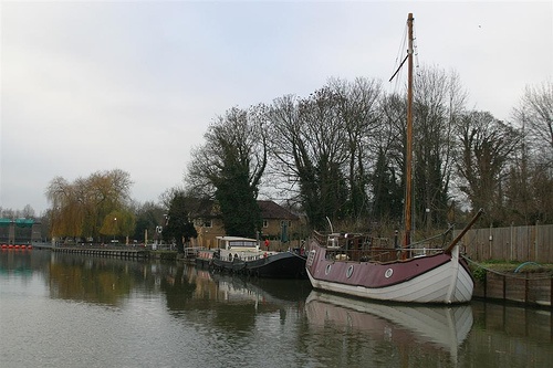
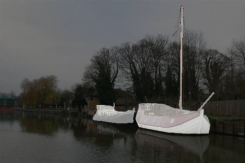
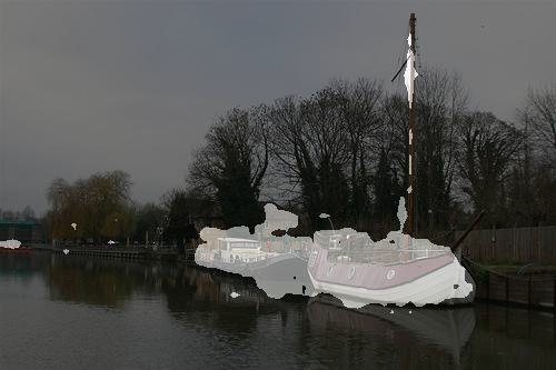
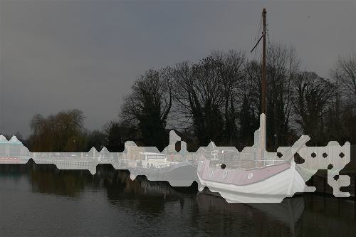
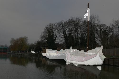
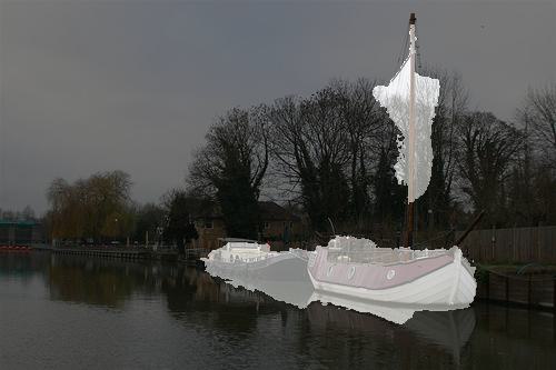
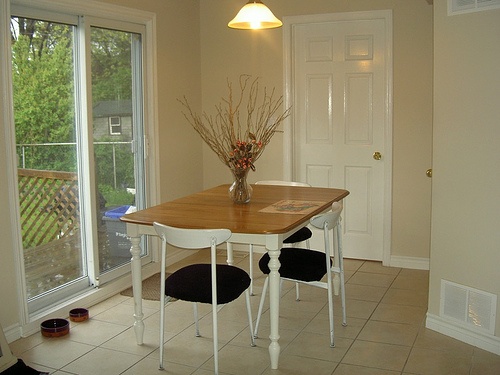
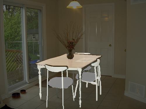
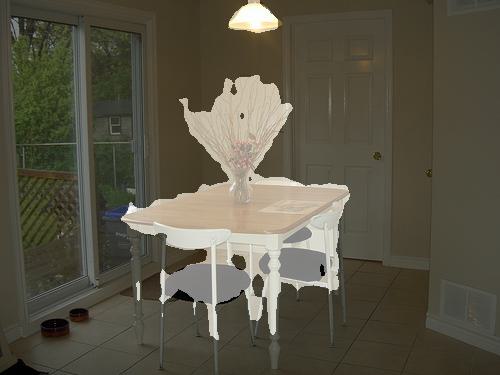
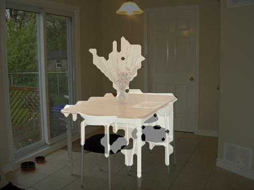
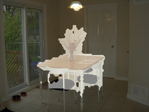
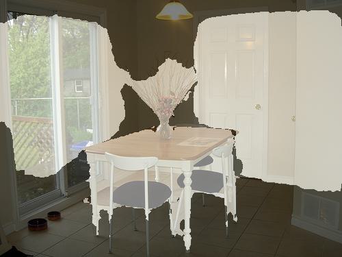
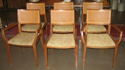
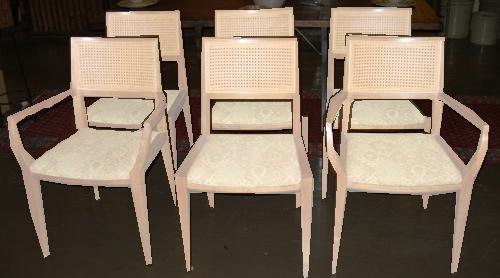
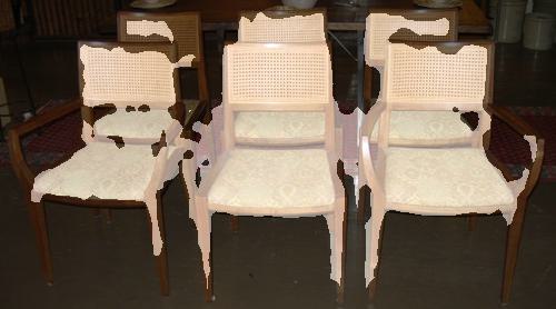
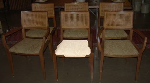
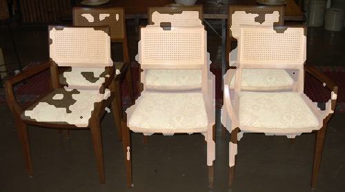
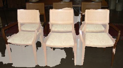
Figure 4: Qualitative results of object localization. We overlay predicted masks generated with our method FOUND, TokenCut [59], SelfMask [44] and FreeSOLO [57] on three images taken from VOC12 [14].

	$\#$ learnable	inference
Method	params.	FPS
LOST [45]	—	64
TokenCut [59]	—	0.4
SelfMask [44]	$\approx 36$M	13
FreeSOLO [57]	$\approx 66$M	13
DINOSAUR [42] – MLP dec. $\ast$	$\geq$ $5$M	—
DINOSAUR [42] – transf. dec.$\ast$	$\geq$ $77$M	—
FOUND	770	80

Table 4: Memory and inference costs. Comparison of the cost of the different methods. ‘$\#$ learnable params.’ excludes weights of the frozen DINO backbone. The FPS measure includes the forward pass through DINO and is computed on a single V100 GPU with PyTorch 1.8.1. ‘$\ast$’: denotes an estimation of the number of learnable parameters for methods without public code.

4.4 Comparison of method costs

We compare FOUND to methods that either do or do not include training, and that have very different costs at inference time. In this section, we highlight the advantage of our method in terms of complexity and speed. FOUND is a segmenter head composed of just $770$ parameters, trained over $2$ epochs on DUTS-TR [55] on a single GPU, and which can infer at $80$ FPS, including the forward pass through DINO, on a V100 GPU. We summarize key numbers in Tab. 4.

First, regarding methods with no training, [59] requires the costly computation of an eigenvector on the Laplacian matrix of the affinity graph, therefore making the method rather slow (0.4 FPS). For the same reasons, [34] runs at equivalent speed to [59]. LOST [45] is almost as fast as us but achieves much lower performance, as seen before.

Second, regarding methods that include training, SelfMask [44] trains a model of $\approx 36$M parameters over $12$ epochs on DUTS-TR [55], by exploiting $27$ mask proposals generated using three different backbones, thus making the training considerably more expensive than ours. FreeSOLO [57] proposes a faster mask proposal extraction step using a DenseCL [58] model based on a ResNet [21] backbone. It then trains a SOLO [56] model ($\approx 65$M learnable parameters) for in total $60$k iterations on 8 GPUs, making it much more expensive to train compared to us.

4.5 Qualitative results

We show visualizations of saliency masks predicted by FOUND and related methods in Fig. 4. We notice that FreeSolo [57] and SelfMask [44] tend to oversegment the objects in all examples, while FOUND yields masks much more accurate with respect to the ground truth. Regarding TokenCut [59], we observe, in the last row of the figure, that it segments just a part of one chair, while FOUND segments all the chair rather accurately. These examples illustrate the efficiency of our method in dealing with multiple objects.

4.6 Ablation study

We present in Tab. 5 an ablation study of our method on the saliency dataset ECSSD [43] — more can be found in Appendix. We measure scores on the unsupervised saliency detection task following the protocol detailed in Sec. 4.2.

Coarse masks.

We evaluate our background discovery method (Sec. 3.1) with and without the attention head reweighting scheme (column R in Tab. 5). We can observe that the reweighting boosts results up to $1$pt when evaluated in a multi-setup mode. We also compare results with and without the application of the post-processing bilateral solver, noted $\zeta()_{p}$, and observe that the refined masks yield better results by $3$pts of IoU in the “single” setting. Such improvements (visualized in Fig. 3 and the supplementary materials) are significant. Overall, our background discovery method (Sec. 3.1) already achieves decent results, particularly when considering the single setup. As discussed before and observed in Fig. 3, our coarse maps cover several objects and do not focus only on the most salient one.

Method	R	$\zeta()_{t}$	$\zeta()_{p}$	Acc	IoU	max $F_{\beta}$
— Coarse masks, no training —
Sec. 3.1 – multi				.876	.627	.689
Sec. 3.1 – multi	✓			.880	.637	.702
Sec. 3.1 – single				.898	.671	.746
Sec. 3.1 – single	✓			.901	.679	.758
Sec. 3.1 – single			✓	.906	.709	.780
Sec. 3.1 – single	✓		✓	.909	.717	.792
— With training —
FOUND – multi	✓			.944	.790	.886
FOUND – multi	✓	✓		.949	.807	.955
FOUND – multi	✓	✓	✓	.951	.813	.935

Table 5: Ablation study. Study of the impact of the different elements in the background discovery step (Sec. 3.1). Results are provided following the unsupervised saliency detection protocol on the ECSSD [43] dataset. $R$ stands for the reweighting of the attention heads. We note $\zeta()_{t}$ and $\zeta()_{p}$ the application of the bilateral solver during training (Eq. 6-7) and as post-processing.

The impact of learning

In the same table, we present results obtained after the training of the single $conv1\times 1$ layer. Training over coarse masks provides a significant boost of more than $15$ IoU pts in the multi setup. This shows that the model learns the concept of foreground objects and smooth results over the dataset. Using the bilateral solver in Eq. 6-7, noted $\zeta()_{t}$, further improves results by 1.7 IoU pts and by an additional .6 pts when also applied as post-processing.

5 Discussion

In this work, we address the problem of unsupervised object localization, that we propose to attack sideways: we look first for the scene background — using self-supervised features — instead of looking for the objects directly. Putting this simple idea at work, we extract coarse masks that encompass most of the background, their complements thus highlighting objects. Using the inverse of the background masks, we train a lightweight segmenter head made of only $770$ learned parameters, which runs at $80$ FPS at inference time — including the forward pass through the backbone — and reaches state-of-the-art results in unsupervised object discovery, unsupervised saliency detection, and unsupervised instance segmentation retrieval.

Acknowledgments

This work was supported by the HPC resources of GENCI-IDRIS in France under the 2021 grant AD011013413, and by the ANR grant MultiTrans (ANR-21-CE23-0032), It was also supported by the Ministry of Education, Youth and Sports of the Czech Republic through the e-INFRA CZ (ID:90140) and by CTU Student Grant SGS21184OHK33T37.

Appendix A Extra details

A.1 During learning

During training, $\zeta()$ is applied at the image resolution. To do so, masks are upsampled to the original image size and the output refined masks are downsampled to the feature map size. The model is trained with the AdamW optimizer provided by PyTorch, with an initial learning rate of $5\text{e}\!-\!2$. We use a simple step scheduler which applies a decay of $0.95$ every $50$ iterations.

A.2 Unsupervised saliency detection

We detail here the different metrics used in the task of unsupervised saliency detection.

The maximal $F_{\beta}$ metric​​​

is the maximum $F_{\beta}$ over various masks which have been binarized using different thresholds. Formally, $F_{\beta}$ is the harmonic mean of precision (P) and recall (R) between a binary mask $M$ and the ground-truth mask $G$, i.e.,

$$F_{\beta}=\frac{(1+\beta^{2})\;\text{P}\times\text{R}}{\beta^{2}\;\text{P}+\text{R}},$$ (8)

where $\beta^{2}$ is the precision weight, set at $0.3$ following [44, 31, 35, 71]. The max $F_{\beta}$ is computed by taking a soft predicted mask $M_{p}\in[0,255]$ and binarizing it using $255$ different thresholds between $0$ and $254$; max $F_{\beta}$ is then the maximum value of $F_{\beta}$ among all the generated binary masks, taken over the whole dataset (single optimal threshold). We noticed in SelfMask’s code that the maximal $F_{\beta}$ is computed with an optimal threshold found for each image rather than over the whole dataset. For this reason, and for a fair comparison, we do not report this original max $F_{\beta}$ in our unsupervised saliency detection table.

The Intersection-over-Union​​​

measures the overlap between foreground regions of a predicted binary mask and the ground-truth mask, averaged over the entire dataset.

The pixel accuracy metric​​​

measures the pixel-wise accuracy between a predicted binary mask $M\in\{0,1\}^{H\times W}$ and the corresponding ground-truth mask $G\in\{0,1\}^{H\times W}$. Formally, it can be defined as:

$$\text{ Acc }=\frac{1}{H\times W}\sum_{i=1}^{H}\sum_{j=1}^{W}\delta_{G_{ij},M_{ij}},$$ (9)

with $\delta$ being the Kroneker-delta function and $G_{ij}$, $M_{ij}$ being the value of the ground-truth and predicted masks at position $(i,j)\in\{1\cdots H\}\times\{1\ldots W\}$.

A.3 Different setups for FreeSOLO

FreeSOLO [57] is a class-agnostic instance segmentation method and outputs several instance masks per image, making it different to other baselines. In order to compare it to our method, we use the code provided online. We follow the original paper to get the prediction masks, i.e., we apply matrix non-maximum suppresion (NMS) [56] and keep masks with a maskness score above $0.7$.

Unsupervised object discovery

We present in Sec. 4.1 of the main paper our unsupervised object discovery protocol. The extraction of the single object box is straightforward for all methods but FreeSOLO [57]. For this method we have considered three setups: (a) merging all instance masks into a single one; (b) keeping only the mask with the highest maskness score; (c) keeping only the mask containing the largest connected component. Best results were achieved with (a) and are reported in the main paper.

Semantic segmentation retrieval

We have performed similar tests with FreeSOLO [57] in the semantic segmentation retrieval task. Additionally to the evaluation setups described in the main paper, we have experimented using two or more instances but without improvements of the results.

A.4 Semantic segmentation retrieval

In the task of unsupervised semantic segmentation retrieval, we consider two setups. One considers that the predicted mask highlights a single object, while the other splits the mask into connected components and treats each component as individual object. In both cases, we compute a per-object feature vector averaged over the pixels of the considered mask. Given a (flattened) binary mask $M\in\{0,1\}^{HW\times 1}$ and corresponding feature tensor $F\in\mathbb{R}^{C\times HW}$ with $C$ the number of channels, we obtain a prototype $P\in\mathbb{R}^{C}$ as

$$P=FM.$$ (10)

These prototypes are first extracted for all train samples and serve as an index for retrieval. Then, to get a label for each val sample, we compute the sample prototype, find nearest neighbors in the train prototypes, and assign it the corresponding label.

Figure 5: Sensitivity to background threshold $\tau$. We report saliency detection results measured on the datasets DUT-OMRON (left) and ECSSD (right) with the IoU metric.

Appendix B Sensitivity to masking method

B.1 Sensitivity to background threshold $\tau$

We investigate here the impact of the background parameter $\tau$ on final results. We report in Fig. 5 saliency detection results. We observe that FOUND is stable to changes of $\tau\!\in\![0.1,0.5]$, with saliency scores varying by at most 0.2 percentage pts on DUT-OMRON and not at all on ECSSD.

method	VOC07	VOC12	COCO20k
TokenCut [59] + T	72.3	75.9	62.7
LOST [45] + T	72.3	76.1	62.8
FOUND (ours)	72.5	76.1	62.9

Table 6: Sensitivity to mask generation method. Unsupervised object discovery results (measured using the CorLoc metric) when using different mask generation strategy to generate the masks $\mathbf{M}^{f}$ refined in our training process. T denotes the training of our segmentation head with the masks $\mathbf{M}^{f}$.

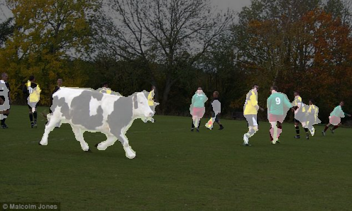
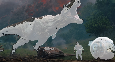
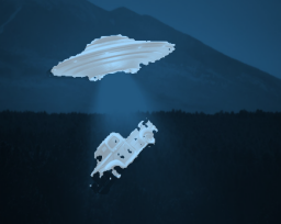
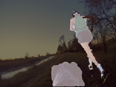
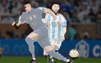
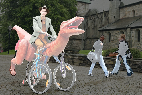
Figure 6: Visualization of FOUND results on images taken from the Internet. Objects out of the domain of ImageNet [11] and DUT-TR [55] (datasets used for training the backbone and our segmentation head), of different scales, and of different shapes are correctly localized.

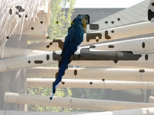
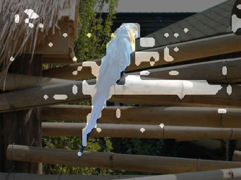
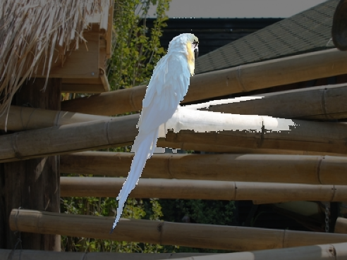
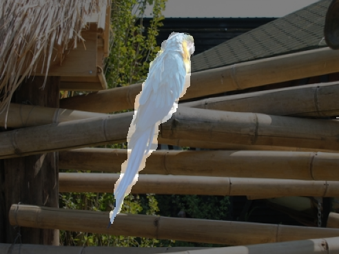
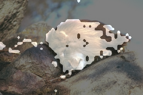
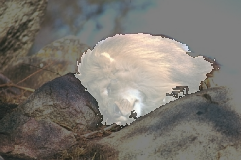
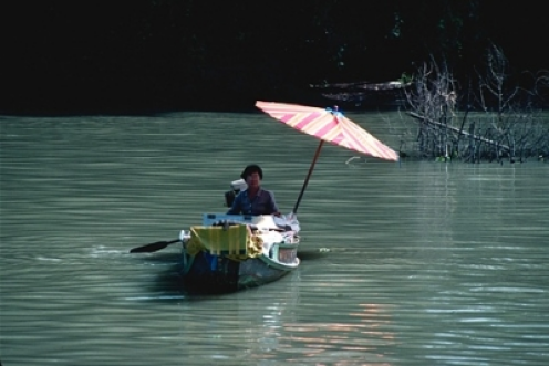
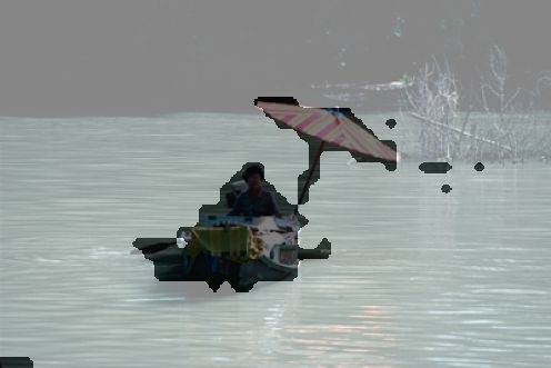
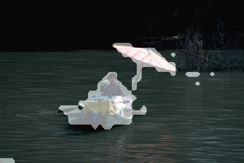
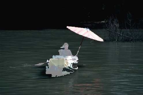
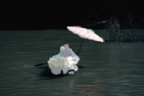
(a) Input image	(b) Coarse background	(c) Coarse foreground	(d) Refined $\zeta(\mathbf{M}^{f})$	(e) Predicted $\mathbf{M}^{s}$
	mask $\mathbf{M}^{b}$	mask $\mathbf{M}^{f}$		(FOUND)

Figure 7: More visualizations of masks generated on images from ECSSD [43] at different stages of our method. We show (a) the input image, (b) the mask $\mathbf{M}^{b}$ extracted using our background discovery step, (c) its inverse $\mathbf{M}^{f}$ used as foreground mask to train our segmenter head, (d) the version refined using a bilateral solver $\zeta(\mathbf{M}^{f})$, and (e) the final output of our trained segmentation head $\mathbf{M}^{s}$.

B.2 Using masks from other methods

We investigate here the performance of our method when considering different mask generators. In particular, we consider the well-known object discovery methods TokenCut [59] and LOST [45] with which we extract the masks $\mathbf{M}^{f}$ that are then refined in our training process (following Sec. 3.2 of the main paper). We present the corresponding unsupervised object discovery results in Tab. 6. They show that our method is agnostic to the mask generator but still performs slightly better with our foreground masks — the complement of the background masks described in Sec. 3.1. It is also to be noted that our method is much faster than TokenCut because we do not need the computation of eigenvectors.

Appendix C Additional qualitative results

We present in this section more visualizations of FOUND results, first on more challenging images (Sec. C.1) and at the different step of our process (Sec. C.2). We then motivate the interest of reweighting the transformer heads (Sec. C.3) via visual illustration. Following we show examples where the application of the bilateral solver impacts negatively the results (Sec. C.4) and some more general failure cases of FOUND (Sec. C.5). We finally provide example of discovered objects as performed in the task of unsupervised object discovery (Sec. C.6).

C.1 Results on generic images from the Internet

We present in Fig. 6 some results of FOUND random images taken from the Internet. These results show the ability of FOUND to discover multiple and diverse objects, both in terms of classes and scales. In particular, dinosaurs and spaceships are not depicted in ImageNet [11] nor DUT-TR [55] and yet FOUND can detect them, showing the ability to discover objects which “are not background.” Moreover, the selected images here are non-object centric and out-of-domain showing the capacity of FOUND to go behond ImageNet-like images.

Input image	Head 0	Head 1	Head 2	Head 3	Head 4	Head 5

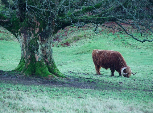
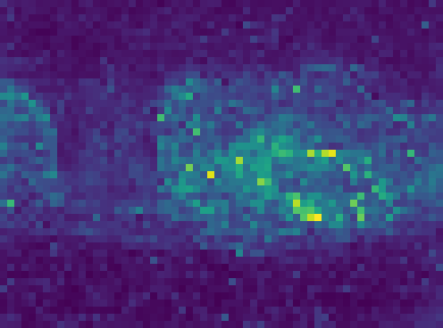
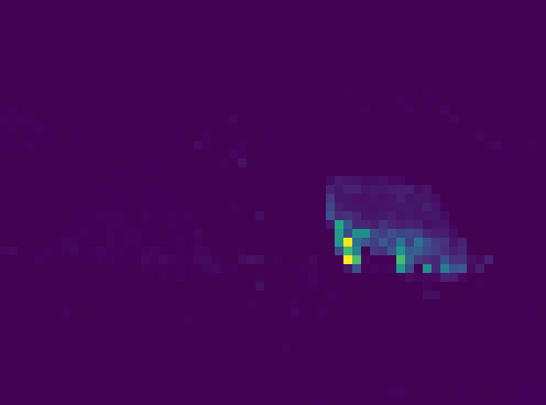
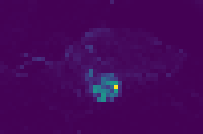
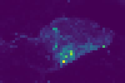
Figure 8: Visualization of self-attention maps obtained with the six different heads in the last attention layer. Results are obtained with a ViT/S-8 trained using DINO [6] applied on an image from VOC07 [13] (first row) and ECSSD [43].

Coarse mask before $\zeta()$	Coarse mask after $\zeta()$
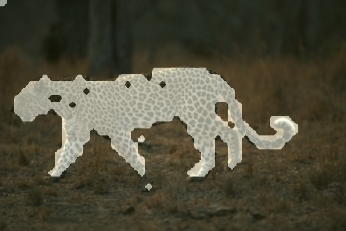
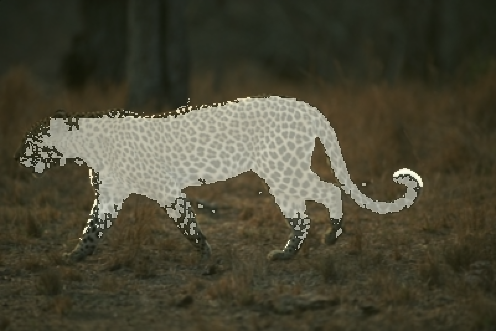
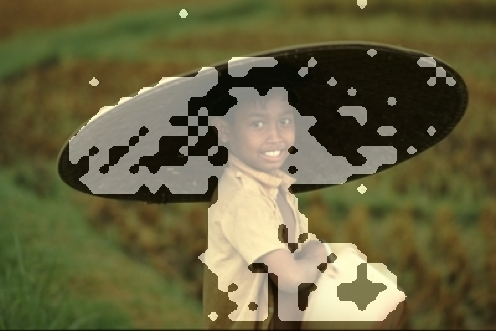
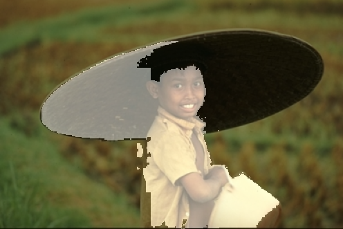
Pred. mask before $\zeta()$	Pred. mask after $\zeta()$

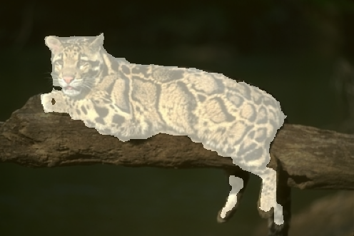
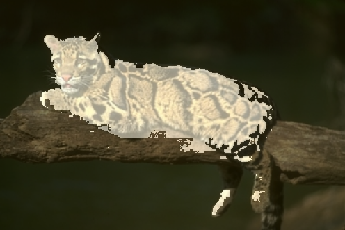
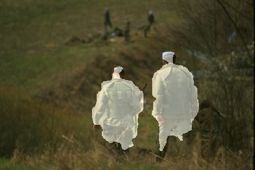
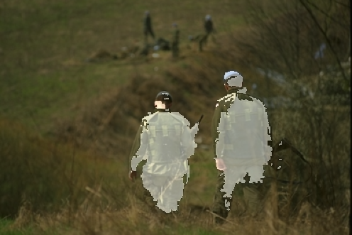
Figure 9: Visualization of the negative impact of the bilateral solver on different ECSSD [43] images.

Input image	FOUND (ours)	SelfMask [44]

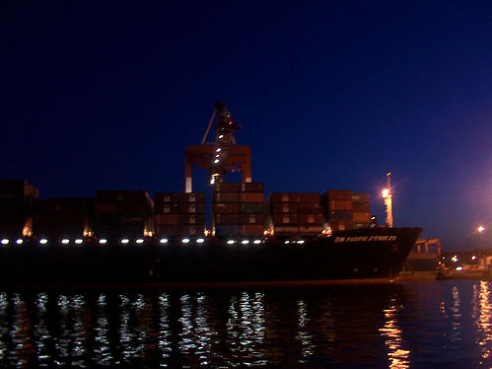
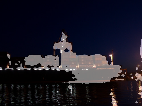
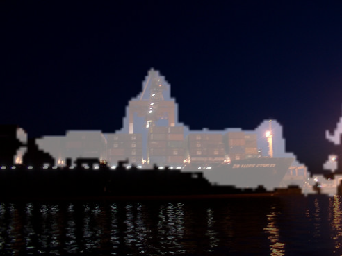
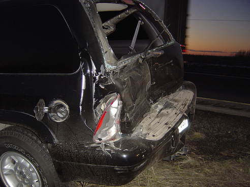
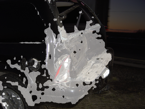
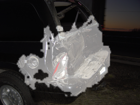
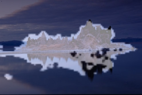
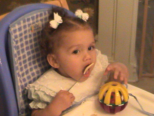
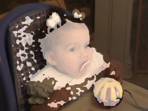
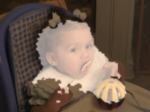
Figure 10: Visualization of failure cases for object localization on images from ECSSD [43], PASCAL VOC07 & VOC12 [13, 14] and DUTS-TE [55] datasets along side results obtained with SelfMask method. No refinement step is applied.

C.2 Visualization of masks at different steps

We provide in Fig. 7 additional visualizations of the masks generated at different steps of our method. We can observe that each step brings an improvement over the previous one. The right-most column presents the final output of FOUND without any refinement.

C.3 Reweighting the attention heads

We provide in Fig. 8 a visualization of the self-attention maps extracted from the last layer of our model. We show the self-attention obtained over the six heads; we can observe that the $4^{\rm th}$ head is noisy. When looking for the background seed, we are looking for the pixel with least attention. Our reweighting scheme helps in reducing the weight given to such noisy heads automatically and improves results, as shown in Tab. 5 of the main paper.

C.4 Potential negative effect of the bilateral solver

While the application of $\zeta()$, the bilateral solver [2], improves results in general (see Fig. 7), there are cases where $\zeta()$ actually degrades the mask quality. We show examples of such cases in Fig. 9 both on coarse masks (rows 1 and 2) and on the final outputs (rows 3 and 4). We can observe that the function amplifies the under-segmentation, e.g., on the hat and the leopard head and legs (row 1 and 2). Moreover, long and thin segments can disappear, e.g., human and animal legs or arms (row 3). Correcting this behaviour would help improving our training and is left for future work.

C.5 Examples of failures cases

We show some failure cases of FOUND in Fig. 10. For these cases, we also present the results obtained with one of the best competitor: SelfMask [44]. We observe that night or dark scenes are challenging (first two rows). Our method tends to under-segment objects but SelfMask has also difficulties in segmenting correctly the main objects in these situation. FOUND, just like SelfMask, is also not robust to reflection on water (third row). Finally, we observe that both methods fail to segment the hair in the fourth columns.

C.6 Unsupervised object discovery results

We present in Fig. 11, qualitative results for the unsupervised single object discovery task (no refinement is applied to the masks). We draw the extracted bounding box on top of the corresponding predicted mask. The conclusions here are similar to those discussed in the main paper. Overall our method segments the objects of interest better and provides cleaner boundaries.

(a) Ground truth	(b) FOUND (ours)	(c) TokenCut [59]	(d) SelfMask [44]	(e) FreeSOLO [57]

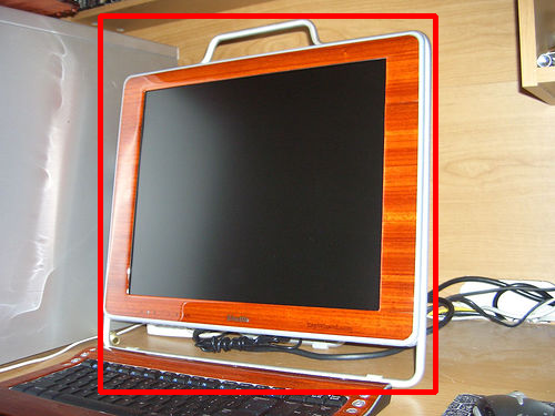
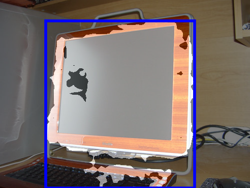
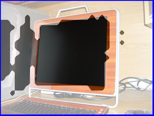
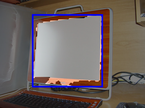
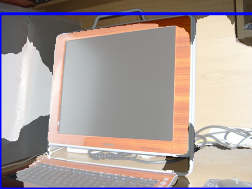
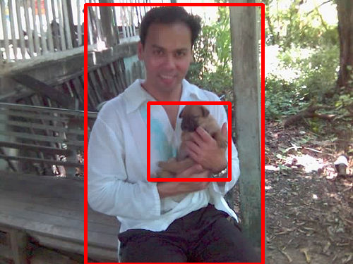
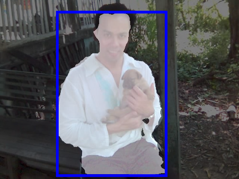
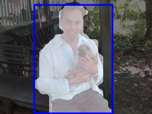
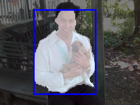
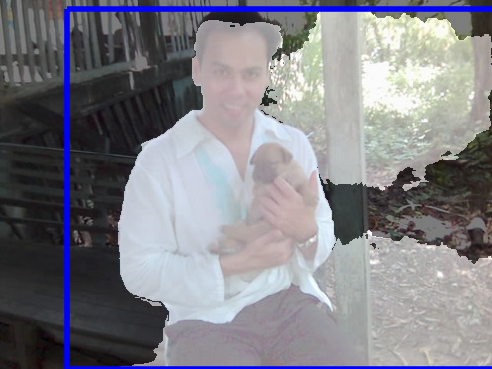
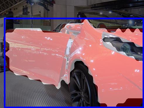
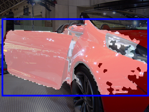
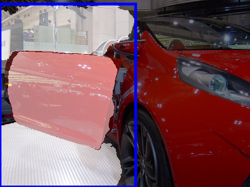
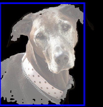
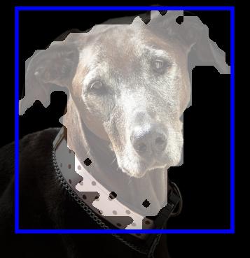
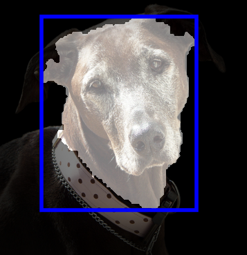
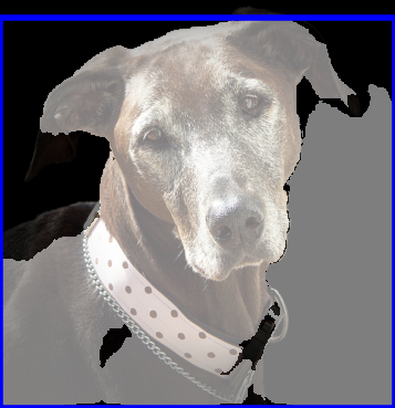
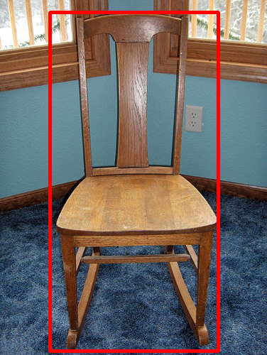
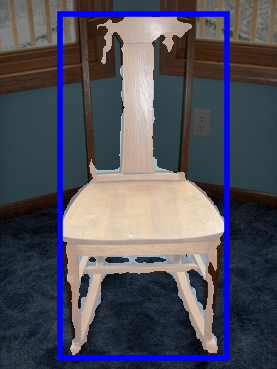
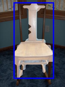
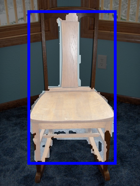
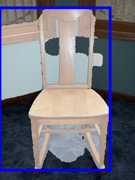
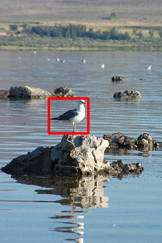
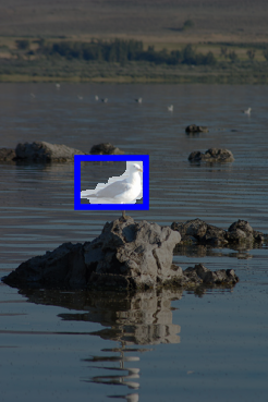
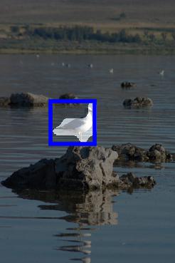
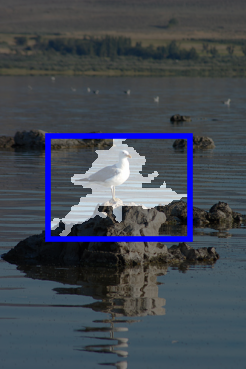
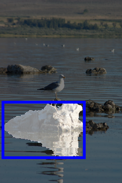
Figure 11: Qualitative results for the task of unsupervised single object discovery on PASCAL VOC12 dataset [14]. We show here masks and boxes extracted as defined in Sec. 4.1. In particular, FOUND is in the single setup (FOUND – single). No refinement step is applied on the masks.

References

- [1] Shir Amir, Yossi Gandelsman, Shai Bagon, and Tali Dekel. Deep vit features as dense visual descriptors. arXiv preprint arXiv:2112.05814, 2021.
- [2] Jonathan T. Barron and Ben Poole. The fast bilateral solver. In ECCV, 2016.
- [3] Ali Borji, Ming-Ming Cheng, Huaizu Jiang, and Jia Li. Salient object detection: A survey. CoRR, abs/1411.5878, 2014.
- [4] Nicolas Carion, Francisco Massa, Gabriel Synnaeve, Nicolas Usunier, Alexander Kirillov, and Sergey Zagoruyko. End-to-end object detection with transformers. In ECCV, 2020.
- [5] Mathilde Caron, Ishan Misra, Julien Mairal, Priya Goyal, Piotr Bojanowski, and Armand Joulin. Unsupervised learning of visual features by contrasting cluster assignments. In NeurIPS, 2020.
- [6] Mathilde Caron, Hugo Touvron, Ishan Misra, Hervé Jégou, Julien Mairal, Piotr Bojanowski, and Armand Joulin. Emerging properties in self-supervised vision transformers. In ICCV, 2021.
- [7] Liang-Chieh Chen, George Papandreou, Iasonas Kokkinos, Kevin Murphy, and Alan L. Yuille. Deeplab: Semantic image segmentation with deep convolutional nets, atrous convolution, and fully connected crfs. IEEE TPAMI, 2018.
- [8] Ting Chen, Simon Kornblith, Mohammad Norouzi, and Geoffrey E. Hinton. A simple framework for contrastive learning of visual representations. In ICML, 2020.
- [9] Xinlei Chen, Haoqi Fan, Ross B. Girshick, and Kaiming He. Improved baselines with momentum contrastive learning. CoRR, abs/2003.04297, 2020.
- [10] Xiaokang Chen, Yuhui Yuan, Gang Zeng, and Jingdong Wang. Semi-supervised semantic segmentation with cross pseudo supervision. In CVPR, 2021.
- [11] Jia Deng, Wei Dong, Richard Socher, Li-Jia Li, Kai Li, and Li Fei-Fei. Imagenet: A large-scale hierarchical image database. In CVPR, pages 248–255, 2009.
- [12] Alexey Dosovitskiy, Lucas Beyer, Alexander Kolesnikov, Dirk Weissenborn, Xiaohua Zhai, Thomas Unterthiner, Mostafa Dehghani, Matthias Minderer, Georg Heigold, Sylvain Gelly, Jakob Uszkoreit, and Neil Houlsby. An image is worth 16x16 words: Transformers for image recognition at scale. In ICLR, 2021.
- [13] M. Everingham, L. Van Gool, C. K. I. Williams, J. Winn, and A. Zisserman. The PASCAL Visual Object Classes Challenge 2007 (VOC2007) Results. http://www.pascal-network.org/challenges/VOC/voc2007/workshop/index.html, 2007.
- [14] M. Everingham, L. Van Gool, C. K. I. Williams, J. Winn, and A. Zisserman. The PASCAL Visual Object Classes Challenge 2012 (VOC2012) Results. http://www.pascal-network.org/challenges/VOC/voc2012/workshop/index.html, 2012.
- [15] Wouter Van Gansbeke, Simon Vandenhende, and Luc Van Gool. Discovering object masks with transformers for unsupervised semantic segmentation. CoRR, abs/2206.06363, 2022.
- [16] Spyros Gidaris, Andrei Bursuc, Gilles Puy, Nikos Komodakis, Matthieu Cord, and Patrick Pérez. Obow: Online bag-of-visual-words generation for self-supervised learning. In CVPR, 2021.
- [17] Spyros Gidaris, Praveer Singh, and Nikos Komodakis. Unsupervised representation learning by predicting image rotations. In ICLR, 2018.
- [18] Mark Hamilton, Zhoutong Zhang, Bharath Hariharan, Noah Snavely, and William T. Freeman. Unsupervised semantic segmentation by distilling feature correspondences. In ICLR, 2022.
- [19] Kaiming He, Xinlei Chen, Saining Xie, Yanghao Li, Piotr Dollár, and Ross B. Girshick. Masked autoencoders are scalable vision learners. In CVPR, 2022.
- [20] Kaiming He, Haoqi Fan, Yuxin Wu, Saining Xie, and Ross B. Girshick. Momentum contrast for unsupervised visual representation learning. In CVPR, 2020.
- [21] Kaiming He, Xiangyu Zhang, Shaoqing Ren, and Jian Sun. Deep Residual Learning for Image Recognition. In CVPR, 2016.
- [22] Laurent Itti, Christof Koch, and Ernst Niebur. A model of saliency-based visual attention for rapid scene analysis. IEEE TPAMI, 1998.
- [23] Peng Jiang, Haibin Ling, Jingyi Yu, and Jingliang Peng. Salient region detection by UFO: uniqueness, focusness and objectness. In ICCV, 2013.
- [24] Tilke Judd, Krista A. Ehinger, Frédo Durand, and Antonio Torralba. Learning to predict where humans look. In ICCV, 2009.
- [25] Yannis Kalantidis, Clayton Mellina, and Simon Osindero. Cross-dimensional weighting for aggregated deep convolutional features. In ECCVW, 2016.
- [26] Gunhee Kim and Antonio Torralba. Unsupervised detection of regions of interest using iterative link analysis. In NeurIPS, 2009.
- [27] Gustav Larsson, Michael Maire, and Gregory Shakhnarovich. Learning representations for automatic colorization. In Bastian Leibe, Jiri Matas, Nicu Sebe, and Max Welling, editors, ECCV, 2016.
- [28] Nianyi Li, Bilin Sun, , and Jingyi Yu. A weighted sparse coding framework for saliency detection. In CVPR, 2015.
- [29] Nianyi Li, Bilin Sun, and Jingyi Yu. A weighted sparse coding framework for saliency detection. In CVPR, 2015.
- [30] Tsung-Yi Lin, Michael Maire, Serge J. Belongie, James Hays, Pietro Perona, Deva Ramanan, Piotr Dollár, and C. Lawrence Zitnick. Microsoft COCO: common objects in context. In ECCV, 2014.
- [31] Jiang-Jiang Liu, Qibin Hou, Ming-Ming Cheng, Jiashi Feng, and Jianmin Jiang. A simple pooling-based design for real-time salient object detection. In CVPR, 2019.
- [32] Yen-Cheng Liu, Chih-Yao Ma, Zijian He, Chia-Wen Kuo, Kan Chen, Peizhao Zhang, Bichen Wu, Zsolt Kira, , and Peter Vajda. Unbiased teacher for semi-supervised object detection. In ICLR, 2021.
- [33] Luke Melas-Kyriazi, Christian Rupprecht, Iro Laina, and Andrea Vedaldi. Finding an unsupervised image segmenter in each of your deep generative models. CoRR, abs/2105.08127, 2021.
- [34] Luke Melas-Kyriazi, Christian Rupprecht, Iro Laina, and Andrea Vedaldi. Deep spectral methods: A surprisingly strong baseline for unsupervised semantic segmentation and localization. In CVPR, 2022.
- [35] Luke Melas-Kyriazi, Christian Rupprecht, Iro Laina, and Andrea Vedaldi. Finding an unsupervised image segmenter in each of your deep generative models. In ICLR, 2022.
- [36] Duc Tam Nguyen, Maximilian Dax, Chaithanya Kumar Mummadi, Thi-Phuong-Nhung Ngo, Thi Hoai Phuong Nguyen, Zhongyu Lou, and Thomas Brox. Deepusps: Deep robust unsupervised saliency prediction via self-supervision. In NeurIPS, 2019.
- [37] Mehdi Noroozi and Paolo Favaro. Unsupervised learning of visual representations by solving jigsaw puzzles. In ECCV, 2016.
- [38] Amin Parvaneh, Ehsan Abbasnejad, Damien Teney, Gholamreza (Reza) Haffari, Anton van den Hengel, and Javen Qinfeng Shi. Active learning by feature mixing. In CVPR, 2022.
- [39] Georgy Ponimatkin, Nermin Samet, Yang Xiao, Yuming Du, Renaud Marlet, and Vincent Lepetit. A simple and powerful global optimization for unsupervised video object segmentation. In WACV, 2023.
- [40] Shaoqing Ren, Kaiming He, Ross B. Girshick, and Jian Sun. Faster R-CNN: towards real-time object detection with region proposal networks. In NeurIPS, 2015.
- [41] Bruno Sauvalle and Arnaud de La Fortelle. Unsupervised multi-object segmentation using attention and soft-argmax. 2023 IEEE/CVF Winter Conference on Applications of Computer Vision (WACV), pages 3266–3275, 2022.
- [42] Maximilian Seitzer, Max Horn, Andrii Zadaianchuk, Dominik Zietlow, Tianjun Xiao, Carl-Johann Simon-Gabriel, Tong He, Zheng Zhang, Bernhard Schölkopf, Thomas Brox, and Francesco Locatello. Bridging the gap to real-world object-centric learning. CoRR, abs/2209.14860, 2022.
- [43] Jianping Shi, Qiong Yan, Li Xu, and Jiaya Jia. Hierarchical image saliency detection on extended CSSD. IEEE TPAMI, 2016.
- [44] Gyungin Shin, Samuel Albanie, and Weidi Xie. Unsupervised salient object detection with spectral cluster voting. In CVPRW, 2022.
- [45] Oriane Siméoni, Gilles Puy, Huy V. Vo, Simon Roburin, Spyros Gidaris, Andrei Bursuc, Patrick Pérez, Renaud Marlet, and Jean Ponce. Localizing objects with self-supervised transformers and no labels. In BMVC, 2021.
- [46] Yonglong Tian, Chen Sun, Ben Poole, Dilip Krishnan, Cordelia Schmid, and Phillip Isola. What makes for good views for contrastive learning? In NeurIPS, 2020.
- [47] Jasper R. R. Uijlings, Koen E. A. van de Sande, Theo Gevers, and Arnold W. M. Smeulders. Selective search for object recognition. IJCV, 2013.
- [48] Wouter Van Gansbeke, Simon Vandenhende, Stamatios Georgoulis, and Luc Van Gool. Unsupervised semantic segmentation by contrasting object mask proposals. In ICCV, 2021.
- [49] Huy V. Vo, Francis R. Bach, Minsu Cho, Kai Han, Yann LeCun, Patrick Pérez, and Jean Ponce. Unsupervised image matching and object discovery as optimization. In CVPR, 2019.
- [50] Huy V. Vo, Patrick Pérez, and Jean Ponce. Toward unsupervised, multi-object discovery in large-scale image collections. In ECCV, 2020.
- [51] Huy V. Vo, Oriane Siméoni, Spyros Gidaris, Andrei Bursuc, Patrick Pérez, and Jean Ponce. Active learning strategies for weakly-supervised object detection. In ECCV, 2022.
- [52] Huy V. Vo, Elena Sizikova, Cordelia Schmid, Patrick Pérez, and Jean Ponce. Large-scale unsupervised object discovery. In NeurIPS, 2021.
- [53] Van Huy Vo, Elena Sizikova, Cordelia Schmid, Patrick Pérez, and Jean Ponce. Large-scale unsupervised object discovery. In M. Ranzato, A. Beygelzimer, Y. Dauphin, P.S. Liang, and J. Wortman Vaughan, editors, Advances in Neural Information Processing Systems, volume 34, pages 16764–16778. Curran Associates, Inc., 2021.
- [54] Andrey Voynov, Stanislav Morozov, and Artem Babenko. Object segmentation without labels with large-scale generative models. In ICML, 2021.
- [55] Lijun Wang, Huchuan Lu, Yifan Wang, Mengyang Feng, Dong Wang, Baocai Yin, and Xiang Ruan. Learning to detect salient objects with image-level supervision. In CVPR, 2017.
- [56] Xinlong Wang, Tao Kong, Chunhua Shen, Yuning Jiang, and Lei Li. Solo: Segmenting objects by locations. In ECCV, 2020.
- [57] Xinlong Wang, Zhiding Yu, Shalini De Mello, Jan Kautz, Anima Anandkumar, Chunhua Shen, and Jose M. Alvarez. Freesolo: Learning to segment objects without annotations. In CVPR, 2022.
- [58] Xinlong Wang, Rufeng Zhang, Chunhua Shen, Tao Kong, and Lei Li. Dense contrastive learning for self-supervised visual pre-training. In CVPR, 2021.
- [59] Yangtao Wang, Xi Shen, Shell Xu Hu, Yuan Yuan, James L. Crowley, and Dominique Vaufreydaz. Self-supervised transformers for unsupervised object discovery using normalized cut. In CVPR, 2022.
- [60] Xiu-Shen Wei, Chen-Lin Zhang, Jianxin Wu, Chunhua Shen, and Zhi-Hua Zhou. Unsupervised object discovery and co-localization by deep descriptor transforming. PR, 2019.
- [61] Yichen Wei, Fang Wen, Wangjiang Zhu, and Jian Sun. Geodesic saliency using background priors. In ECCV, 2012.
- [62] Tong Wu, Junshi Huang, Guangyu Gao, Xiaoming Wei, Xiaolin Wei, Xuan Luo, and Chi Harold Liu. Embedded discriminative attention mechanism for weakly supervised semantic segmentation. In CVPR, 2021.
- [63] Qiong Yan, Li Xu, Jianping Shi, and Jiaya Jia. Hierarchical saliency detection. In CVPR, 2013.
- [64] Qiong Yan, Li Xu, Jianping Shi, and Jiaya Jia. Hierarchical saliency detection. In CVPR, 2013.
- [65] Chuan Yang, Lihe Zhang, Huchuan Lu, Xiang Ruan, and Ming-Hsuan Yang. Saliency detection via graph-based manifold ranking. In CVPR, 2013.
- [66] Tianning Yuan, Fang Wan, Mengying Fu, Jianzhuang Liu, Songcen Xu, Xiangyang Ji, and Qixiang Ye. Multiple instance active learning for object detection. In CVPR, 2021.
- [67] Andrii Zadaianchuk, Matthaeus Kleindessner, Yi Zhu, Francesco Locatello, and Thomas Brox. Unsupervised semantic segmentation with self-supervised object-centric representations. CoRR, abs/2207.05027, 2022.
- [68] Dingwen Zhang, Junwei Han, and Yu Zhang. Supervision by fusion: Towards unsupervised learning of deep salient object detector. In ICCV, 2017.
- [69] Jing Zhang, Tong Zhang, Yuchao Dai, Mehrtash Harandi, and Richard I. Hartley. Deep unsupervised saliency detection: A multiple noisy labeling perspective. In CVPR, 2018.
- [70] Runsheng Zhang, Yaping Huang, Mengyang Pu, Jian Zhang, Qingji Guan, Qi Zou, and Haibin Ling. Object discovery from a single unlabeled image by mining frequent itemsets with multi-scale features. TIP, 29, 2020.
- [71] Jiaxing Zhao, Jiang-Jiang Liu, Deng-Ping Fan, Yang Cao, Jufeng Yang, and Ming-Ming Cheng. Egnet: Edge guidance network for salient object detection. In ICCV, 2019.
- [72] Jinghao Zhou, Chen Wei, Huiyu Wang, Wei Shen, Cihang Xie, Alan L. Yuille, and Tao Kong. Image BERT pre-training with online tokenizer. In ICLR, 2022.
- [73] Wangjiang Zhu, Shuang Liang, Yichen Wei, and Jian Sun. Saliency optimization from robust background detection. In CVPR, 2014.
- [74] Wangjiang Zhu, Shuang Liang, Yichen Wei, and Jian Sun. Saliency optimization from robust background detection. In CVPR, 2014.
- [75] Wangjiang Zhu, Shuang Liang, Yichen Wei, and Jian Sun. Saliency optimization from robust background detection. In CVPR, 2014.
- [76] Lawrence Zitnick and Piotr Dollár. Edge boxes: Locating object proposals from edges. In ECCV, 2014.