CREPE: Can Vision-Language Foundation Models Reason Compositionally?

Abstract

A fundamental characteristic common to both human vision and natural language is their compositional nature. Yet, despite the performance gains contributed by large vision and language pretraining, we find that—across 7 architectures trained with 4 algorithms on massive datasets—they struggle at compositionality. To arrive at this conclusion, we introduce a new compositionality evaluation benchmark, CREPE, which measures two important aspects of compositionality identified by cognitive science literature: systematicity and productivity. To measure systematicity, CREPE consists of a test dataset containing over $370K$ image-text pairs and three different seen-unseen splits. The three splits are designed to test models trained on three popular training datasets: CC-12M, YFCC-15M, and LAION-400M. We also generate $325K$, $316K$, and $309K$ hard negative captions for a subset of the pairs. To test productivity, CREPE contains $17K$ image-text pairs with nine different complexities plus $183K$ hard negative captions with atomic, swapping and negation foils. The datasets are generated by repurposing the Visual Genome scene graphs and region descriptions and applying handcrafted templates and GPT-3. For systematicity, we find that model performance decreases consistently when novel compositions dominate the retrieval set, with Recall@1 dropping by up to $12\%$. For productivity, models’ retrieval success decays as complexity increases, frequently nearing random chance at high complexity. These results hold regardless of model and training dataset size.

Figure 1: We introduce CREPE, a benchmark to evaluate whether vision-language foundation models demonstrate two fundamental aspects of compositionality: systematicity and productivity. To evaluate systematicity, CREPE utilizes Visual Genome and introduces three new test datasets for the three popular pretraining datasets: CC-12M, YFCC-15M, and LAION-400M. These enable evaluating models’ abilities to systematically generalize their understanding to seen compounds, unseen compounds, and even unseen atoms. To evaluate productivity, CREPE introduces examples of nine complexities, with three types of hard negatives for each.

1 Introduction

Compositionality, the understanding that “the meaning of the whole is a function of the meanings of its parts” [13], is held to be a key characteristic of human intelligence. In language, the whole is a sentence, made up of words. In vision, the whole is a scene, made up of parts like objects, their attributes, and their relationships [41, 37]. Through compositional reasoning, humans can understand new scenes and generate complex sentences by combining known parts [35, 32, 7]. Despite compositionality’s importance, there are no large-scale benchmarks directly evaluating whether vision-language models can reason compositionally. These models are pretrained using large-scale image-caption datasets [88, 75, 77], and are already widely applied for tasks that benefit from compositional reasoning, including retrieval, text-to-image generation, and open-vocabulary classification [12, 68, 73]. Especially as such models become ubiquitous “foundations” for other models [6], it is critical to understand their compositional abilities.

Figure 2: An overview of the systematicity retrieval set generation process. First, a model’s image-caption training set is parsed to identify what atoms and compounds the model has seen. Then, an evaluation set is divided into three compositional splits according to whether the model has seen all the compounds (Seen Compounds), only all the atoms of the caption (Unseen Compounds), or neither (Unseen Atoms). Finally, hard negative captions HN-Atom and HN-Comp are generated for the hard negatives retrieval set $\mathcal{D}_{test}^{HN}$ .

Previous work has evaluated these models using image-text retrieval [38, 67, 98]. However, the retrieval datasets used either do not provide controlled sets of negatives [53, 88] or study narrow negatives which vary along a single axis (e.g. permuted word orders or single word substitutions as negative captions) [61, 89, 78, 24]. Further, these analyses have also not studied how retrieval performance varies when generalizing to unseen compositional combinations, or to combinations of increased complexity.

We introduce CREPE (Compositional REPresentation Evaluation): a new large-scale benchmark to evaluate two aspects of compositionality: systematicity and productivity (Figure 1). Systematicity measures how well a model is able to represent seen versus unseen atoms and their compositions. Productivity studies how well a model can comprehend an unbounded set of increasingly complex expressions. CREPE uses Visual Genome’s scene graph representation as the compositionality language [41] and constructs evaluation datasets using its annotations. To test systematicity, we parse the captions in three popular training datasets, CC-12M [10], YFCC-15M [88], and LAION-400M [75], to identify atoms (objects, relations, or attributes) and compounds (combinations of atoms) present in each dataset. For each training set, we curate corresponding test sets containing $385K$, $385K$ and $373K$ image-text pairs respectively, with splits checking generalization to seen compounds, unseen compounds, and unseen atoms. To test productivity, CREPE contains $17K$ image-text pairs split across nine levels of complexity, as defined by the number of atoms present in the text. Examples across all datasets are paired with various hard negative types to ensure the legitimacy of our conclusions.

Our experiments—across 7 architectures trained with 4 training algorithms on massive datasets—find that vision-language models struggle at compositionality, with both systematicity and productivity. We present six key findings: first, our systematicity experiments find that models’ performance consistently drops between seen and unseen compositions; second, we observe larger drops for models trained on LAION-400M (up to a $12\%$ decrease in Recall@1); third, our productivity experiments indicate that retrieval performance degrades with increased caption complexity; fourth, we find no clear trend relating training dataset size to models’ compositional reasoning; fifth, model size also has no impact; finally, models’ zero-shot ImageNet classification accuracy correlates only with their absolute retrieval performance on the systematicity dataset but not systematic generalization to unseen compounds or to productivity.

2 Related Work

Our work lies within the field of evaluating foundation models. Specifically, we measure visio-linguistic compositionality. To do so, we create a retrieval benchmark with hard negatives.

Contrastive Image-Text Pretraining. The recently released contrastively trained CLIP model [67] has catalyzed a wide array of work at the intersection of Computer Vision and Natural Language Processing. Since its release, CLIP has enabled several tasks, ranging from semantic segmentation to image captioning, many of which have remarkable zero-shot capability [67, 45, 87, 84, 18, 14]. CLIP has been used as a loss function within image synthesis applications [54, 64, 95, 52, 100, 34], acted as an automated evaluation metric [62, 25], used successfully as a feature extractor for various vision and language tasks [79], and incorporated into architectures for various tasks including dense prediction and video summarization [65, 69, 51, 81, 60, 80]. This success has also encouraged the design of other contrastive vision and language pretraining algorithms for image [48, 21, 56, 17, 50, 97, 96, 82, 47] and video domains [46, 91, 94]. Our work evaluates how well such contrastively trained models capture a fundamental property present in human vision and language: compositionality.

Compositionality. Compositionality allows us to comprehend an infinite number of scenes and utterances [43]. For an AI model, compositionality would not only allow for systematic, combinatorial generalization, but would also confer benefits such as controllability [6]. This promise prompted a wealth of work on both designing [28, 2, 30] and evaluating  [31, 22, 42, 85, 20] compositional models. In our work, we focus on two aspects of compositionality: systematicity and productivity. While there is a plethora of benchmarks for systematic generalization within Computer Vision [39, 3, 5, 22] and Machine Learning [42, 72, 40], the subject has been almost unexplored for vision-language models, largely due to lack of benchmarks complementary to the different large-scale training datasets. To address this, CREPE provides a benchmark with three different datasets to evaluate the compositional generalization of vision-language models. Productivity, on the other hand, has been studied only for specialized tasks [22] or toy domains [42, 72, 32]. CREPE evaluates productivity by using an image-text retrieval task featuring captions of varying compositional complexity.

Evaluation with hard negatives. Like us, past work evaluating models has commonly designed tasks featuring hard negatives to isolate particular model capabilities while overcoming the limitations of prior evaluation tasks. Using atomic foils that replace an atom in the image or text with a distractor has been the most common strategy [78, 29, 24, 11, 5, 63, 61]. Notably, Park et al. [63] targets verbs and person entities in videos; COVR [5] studies question answering with distractor images; VALSE [61] targets linguistic phenomena such as existence, cardinality and the recognition of actions and spatial relationships. Another strategy has been to swap atoms within a caption to test whether models behave akin to a bag-of-words [1, 61, 89]. In particular, Winoground [89] introduces a set of $800$ human edited negatives to evaluate compositionality; it is the closest related work to us. We complement Winoground by scaling it up by three orders of magnitude, by decomposing compositionality into systematicity and productivity, and by studying a variety of different types of hard negatives.

Figure 3: An overview of the productivity retrieval set generation process. By performing random walks on the scene graphs of an evaluation dataset, we generate subgraphs of various complexities. Then, for complexities $n\in\{4,,5\dots,12\}$ and three hard negative types, we populate the retrieval set $\mathcal{D}_{test}^{HN}$ by generating a ground truth caption for each $n$-subgraph and hard negatives for each caption.

3 Compositional evaluation

The following section builds from the formally vacuous principle of compositionality to a well-defined evaluation scheme [32]. First, we establish the syntax and semantics of the composed language (Section 3.1). Then, we define expected behaviors from a model that achieves comprehension of said language ( 3.2, 3.3). Finally, we establish how to empirically measure those behaviors via retrieval ( 3.4).

3.1 Compositional language of visual concepts

To evaluate vision-language models, we find that a compositional language consisting of scene graph visual concepts is an appropriate foundation [41]. Accordingly, an atom $A$ is defined as a singular visual concept, corresponding to a single scene graph node. Atoms are subtyped into objects $A_{o}$, relationships $A_{r}$, and attributes $A_{a}$. A compound $C$ is defined as a primitive composition of multiple atoms, which corresponds to connections between scene graph nodes. Visual concepts admit two compound types: the attachment of attribute to objects (“black dog”) $C_{ao}$, and the attachment of two objects via a relationship (“man hugs child”) $C_{oro}$.

The composition of these compounds form subgraphs $S$, which can be translated to natural language captions $T$. Conversely, captions $T$ derived from image-text datasets $\mathcal{D}$ can be parsed to become scene graphs $S$. This extensible language is capable of capturing a number of linguistic phenomena identified in existing literature [85, 61], including the existence of concepts (“a photo with flowers”), spatial relationships (“a grill on the left of a staircase”), action relationships (“a person throwing a frisbee”), prepositional attachment (“A bird with green wings”), and negation (“There are no trucks on the road”). Furthermore, while this study focuses on visual concepts, scene graphs featuring common-sense relationships or other more abstract concepts can be designed; therefore, our methodology is widely applicable [74].

Table 1: We summarize the sizes of the eight evaluation datasets we create for systematicity and productivity evaluation.

	Systematicity								Productivity
	$\mathcal{D}_{test}^{RAW}$ (# of image-text pairs)				$\mathcal{D}_{test}^{HN}$ (# of texts)				$\mathcal{D}_{test}^{RAW}$		$\mathcal{D}_{test}^{HN}$
Training data	CC-12M	YFCC-15M	LAION-400M		CC-12M	YFCC-15M	LAION-400M		Any		Any
Dataset size	385,777	385,777	373,703		325,523	316,668	309,342		17,553		183,855

3.2 Systematicity

With our compositional language in place, we now define two dimensions of compositionality—systematicity and productivity—which we adapt to vision-language representations. Systematicity evaluates a model’s ability to systematically recombine seen atoms in compounds. Concretely, let $\textsc{Seen}(A,D)$ denote if an atom is seen in a training dataset $\mathcal{D}$, namely $\exists(I,S)\in\mathcal{D}:A\in S$, and $\textsc{Seen}(C,D)$ denote if a compound is seen in a dataset $\mathcal{D}$, namely $\exists(I,S)\in\mathcal{D}:C\subseteq S$. To evaluate systematicity, we define three compositional splits: Seen Compounds (SC), Unseen Compounds (UC) and Unseen Atoms (UA). SC is the split where all compounds (and thus all atoms) of every caption have been seen in the training dataset, i.e. $\mathcal{D}_{\textsc{SC}}=\{(I,S)\in\mathcal{D}_{test}\,|\,\forall C\subseteq S:\textsc{Seen}(C,\mathcal{D}_{train})\}$. UC is the split where, for each caption, all atoms have been seen but at least one compound has NOT, i.e. $\mathcal{D}_{UC}=\{(I,S)\in\mathcal{D}_{test}\,|\,(\forall A\in S:\textsc{Seen}(A,\mathcal{D}_{train})\land(\exists C\subseteq S:\neg\mathrm{Seen}(C,\mathcal{D}_{train}))\}$. UA is the split where each caption contains at least one atom that has NOT been seen, i.e. $\mathcal{D}_{UA}=\{(I,S)\in\mathcal{D}_{test}\,|\,\exists A\in S:\neg\textsc{Seen}(A,\mathcal{D}_{train})\ \}$.

3.3 Productivity

Productivity refers to a capacity to comprehend an unbounded set of expressions. Since the set of atoms in any dataset is finite, a reasonable substitute for testing unbounded comprehension is testing comprehension over increasingly complex scenes. Now, an image $I$ does not have a notion of complexity, since it is theoretically infinitely describable; on the other hand, we can define a notion of complexity for a caption $T$: the number of atoms in its corresponding scene graph $|S_{T}|$. Therefore, a productive vision-language model should be able to match a given image to the correct corresponding caption, regardless of that caption’s complexity. To evaluate productivity, we define a range of productivity complexity (in our case, $n=4,5,\dots,12$). We need splits of the evaluation dataset based on these complexities, where image-text pairs in a given split have a fixed complexity $n$, and evaluate a model’s performance over each split.

3.4 Compositional evaluation via retrieval

We evaluate compositional reasoning using zero-shot image-to-text and text-to-image retrieval. This formulation probes the representation space as directly as possible and is already the most common evaluation method for vision-language foundation models [67]. Theoretically, any existing image-text dataset can be used as retrieval sets for our evaluation. However, one challenging limitation in existing datasets renders the metrics evaluated on them inaccurate. Consider using an image query of a “plant inside a yellow vase on top of a black television.” Retrieving unintended alternative positives (e.g. “a black television”) is not necessarily incorrect. Similarly, if no other texts in the retrieval set contain a “plant” and a “television”, retrieving the correct text doesn’t suggest that the model comprehends the image. Ideally, to properly evaluate a model, the retrieval dataset should contain hard negatives for every query. A hard negative is a caption that does not faithfully represent the corresponding image, and differs from the ground truth caption by some minimal atomic shift. A example hard negative for the query above is “man inside a yellow vase on top of a black television.” By erring in a single, granular syntactic or semantic fashion, hard negatives allow for variations in retrieval performance to be attributable to a specific failure mode of a model’s compositional comprehension (see Appendix). We address this need for a new benchmark dataset to evaluate the systematicity and productivity of vision-language models.

4 CREPE: a large-scale benchmark for vision-language compositionality

There are several challenges to creating image-text retrieval datasets that evaluate compositional systematicity and productivity. For systematicity, the primary challenge lies in parsing the training dataset for seen atoms and compounds in order to split the data into the three compositional splits. For productivity, the major challenge is generating image-text pairs across different text complexities for the retrieval sets. For both datasets, it is crucial to enumerate different types of hard negatives, and to design an automated hard negative generator which ensures the incorrectness of the negatives it generates. We detail our methods for tackling these challenges for future efforts that attempt to create similar benchmarks for other training datasets.

4.1 Creating systematicity datasets

To create the three systematicity splits—SC, SA, UA—we parse a given training dataset $\mathcal{D}$ into its constituent atoms and compounds, filter low-quality data, and generate hard negatives (Figure 2).

Parsing a dataset into atoms and compounds Since we utilize the scene graph representation as our compositional language, we use the Stanford Scene Graph Parser [76, 93] to parse texts in $\mathcal{D}_{train}$ into their corresponding scene graphs with objects, attributes and relationships. Since the parser only parses for objects and relationships, we further extract the attributes from the text via spaCy’s natural language processing parser by identifying adjective part-of-speech tags. These connected objects, attributes, and relationships constitute our seen atoms and compounds. Similarly, we parse a given $\mathcal{D}_{test}$ and divide all the image-text pairs into the three splits based on the presence of unseen atoms and/or compounds in the parsed training set. Details on the quality of the scene graph parser can be found in the Appendix.

Filtering low-quality data We perform the following filtering steps on the image-text pairs in all splits: we only keep region crops which have an area greater than or equal to $40K$ pixels, occupy at least $10\%$ of the whole image, and whose width-to-height ratio is between $0.5$-$2.0$. We only include text which have at least $2$ atoms and $1$ compound and de-duplicate text using their corresponding scene graphs.

Generating hard negatives We introduce two types of hard negatives: HN-Atom and HN-Comp. HN-Atom replaces $A_{a}$, $A_{o}$, or $A_{r}$ in the text with an atomic foil. For example, for the caption “a grill on top of the porch”, one HN-Atom can be “a grill underneath the porch”, where the $A_{r}$ “on top of” is replaced by “underneath”. Since captions and scene graphs are not exhaustive, this replacement must be done carefully. For example, if a dog is white and furry, but only “white” is annotated, replacing the atom “white” with “furry” would result in a correct caption. To minimize errors, we employ WordNet [59] to pick replacement atoms that are either antonyms (“black dog”) or share the same grand-hypernym (“pink dog") with respect to the original atom. Furthermore, we use BERT to select the most sensical negatives for each ground truth caption [15, 61]. HN-Comp concatenates two compound foils where each contains an atomic foil. For instance, one HN-Comp of the caption “a pink car” can be “a blue car and a pink toy”, where “blue” and “toy” are the atomic foils in the two compounds foils “blue car” and “pink toy”. We only generate negatives for one-compound examples for systematicity evaluation, as productivity covers complex captions with more atoms.

Figure 4: Systematicity analysis. We plot models’ recall@1 on the Seen Compounds vs. Unseen Compounds split of the systematicity retrieval set with hard negatives HN-Atom, HN-Comp and both types. We observe a consistent drop in models’ performance from the SC to UC split when the retrieval set contains HN-Atom or both types, and little to no difference when it contains only HN-Comp.

4.2 Creating productivity datasets

We first generate ground truth captions for scene graphs of varying complexity, filter for data quality, and then generate hard negatives for each example (Figure 3).

Generating captions We systematically generate captions of different atom counts for each image. Given a scene graph, we perform a random walk of length $n$ through the graph to generate a subgraph. Each subgraph corresponds to a specific region of the image, determined by the union of the bounding boxes of the subgraph atoms. We filter out low-quality regions using the same process as systematicity with additional deduplication on patches that overlap by $\geq 75\%$. For simple subgraphs ($n=4$), we produce captions using handcrafted templates. For larger subgraphs ($n\geq 5$), we leverage GPT-3 [8] (text-davinci-002) to generate captions based on a text description of the scene graph, which lists all objects and relationships. We prompt GPT-3 using 5 manually written captions per complexity, filtering out captions where GPT-3 errs and omits atoms from the subgraph during generation (see more details in Appendix).

Generating hard negatives For productivity, we employ three hard negatives types (HN-Atom from systematicity, HN-Swap, and HN-Neg) corresponding to three hypothesized model error modes. First, as a caption’s complexity increases, a model may begin to ignore individual atoms. HN-Atom randomly selects an atom from the caption and replaces it with an incorrect atom. Second, as a caption’s complexity increases, a model may treat captions as “bags of words”, ignoring syntactic connections built out of word order. A swap hard negative (HN-Swap) accordingly permutes atoms of the same subtype in a caption. This hard negative is similar to Winoground [89], but in the context of varying caption complexity. On top of Wordnet, we use entailment with RoBERTa to further filter errant HN-Swap hard negatives [55]. Finally, as a caption’s complexity increases, a model may begin to lose comprehension of negations. A negation hard negative (HN-Neg) either negates the entire caption or a specific atom. Refer to the Appendix for details on generating HN-Swap and HN-Neg.

Figure 5: Productivity Analysis. We plot models’ Recall@1 on the hard negatives retrieval set against complexity, averaged across all models pretrained on all three training datasets. We find that models’ ability to retrieve the ground-truth degrades as complexity increases.

Figure 6: Productivity Analysis on Additional Foundation Vision-language Models. We plot models’ Recall@1 on the productivity hard negatives retrieval set against complexity, where OpenAI CLIP’s performance is averaged across five models RN50, RN101, ViT-B-16, ViT-B-32 and ViT-L-14. We find that all models’ retrieval performance decreases as complexity increases in both the HN-ATOM and HN-SWAP retrieval sets. For the HN-NEG set, all models except for CLIP either drop in performance or remain at random chance.

4.3 The final benchmark datasets

For both productivity and systematicity, we generate two test datasets: $\mathcal{D}_{test}^{HN}$, which contains image-ground truth text pairs along with all generated hard negatives, and $D_{test}^{RAW}$, which contains only image-ground truth text pairs. To measure the data quality, we randomly sample $2\%$ of productivity ground truth captions generated by GPT-3 and $1\%$ of the queries in the productivity and systematicity $\mathcal{D}_{test}^{HN}$ sets for manual human verification. We assign $2$ annotators to each set and measure both generated quality and intra-annotator agreement. $87.9\%$ of sampled productivity ground truth captions generated by GPT-3 are rated as faithful to the image, with an average pairwise annotator agreement of $88.8\%$. $83.7\%$ of productivity and $86.0\%$ of systematicity hard negatives were rated as genuine negatives (i.e. made factually incorrect statements about the image), with pairwise annotator agreements of $84.3\%$ and $83.7\%$ respectively.

5 Experiments

We present our experimental setup and results with six takeaways. First, our systematicity experiments show performance decreases consistently on compounds unseen in training. Second, the greatest drop between splits occurs for models trained on LAION-400M. Third, our productivity results reveal models’ retrieval performance decays with increasing complexity. Fourth, we find that dataset size has no impact on compositionality. Fifth, we find no clear trend relating model size to compositionality. Finally, models’ zero-shot ImageNet classification accuracy correlates with retrieval performance on the systematicity dataset but not systematic generalization to the UC split or productivity.

Datasets. We utilize Visual Genome to create our test datasets. For systematicity, image patches and corresponding spelling-corrected region descriptions are used. We provide three different splits for $\mathcal{D}_{test}^{HN}$, for three training datasets: CC-12M, YFCC-15M and LAION-400M. For productivity, Visual Genome’s image-scene graph pairs are used to create captions and hard negatives for $\mathcal{D}_{test}^{RAW}$ and $\mathcal{D}_{test}^{HN}$ (Table 1).

Models. We firstly evaluate seven vision-language models pretrained with contrastive loss [83] across three commonly used image-text datasets: Conceptual Captions 12M (CC-12M) [10], a subset of the YFCC100M dataset (YFCC-15M) [88, 67] and LAION-400M [75]. We limit our evaluation to models openly released in the OpenCLIP repository [33] for systematicity evaluation. These include ResNet (RN) [23] and Vision Transformer (ViT) [16] encoders of different sizes: RN50, RN101, ViT-B-16, ViT-B-16-plus-240, ViT-B-32 and ViT-L-14. Additionally, since productivity evaluation is not restricted to models that were trained on publicly released datasets, we conduct productivity evaluation on other foundation vision-language models as well. Specifically, we consider OpenAI’s CLIP [67] with ResNet and ViT backbones, CyCLIP [21] (a variant of CLIP introducing auxiliary losses that regularize the gap in similarity scores between mismatched pairs, trained on Conceptual Captions 3M [77] with a ResNet-50 [23] backbone), ALBEF [48] (additionally trained with a masked language modeling and image-text matching loss) and FLAVA [82] (which further adds unimodal losses for image and text domains).

Retrieval. For $\mathcal{D}_{test}^{HN}$, we perform image-to-text retrieval and stratify results by split and hard negative type. For systematicity, the splits are $SC$, $UC$, and $UA$; for productivity, the splits are by caption complexity $n$ (denoted $\mathcal{D}_{test}^{HN,n}$). Each retrieval task is between one image and its ground truth caption plus $h$ hard negatives of a single type (see Appendix). We adopt commonly used retrieval metrics Recall@1, 3, 5 and Average Recall@K. For $\mathcal{D}_{test}^{RAW}$, retrieval experiments are described in the Appendix.

Figure 7: A plot of ImageNet zero-shot top-1 accuracy vs. Recall@1 on CREPE’s systematicity hard-negative sets. We observe a strong correlation for both splits on HN-ATOM and HN-COMP.

Figure 8: A plot showing the correlation between zero-shot top-1 accuracy on ImageNet and Recall@1 on CREPE’s productivity hard negative sets for complexities of $4,8$, and $12$. Overall, we find a strong correlation between ImageNet accuracy and Recall@1 on our productivity HN-Neg ($R^{2}>0.78$) and HN-Atom ($R^{2}>0.54$) sets and weak to no correlation on HN-Swap.

5.1 Systematicity evaluation

Model performance on the $\mathcal{D}_{test}^{HN}$ dataset for systematicity decreases monotonically when compounds are unseen.

We first observe a monotonic decrease in recall@1 from the Seen Compounds to the Unseen Compounds split on the systematicity $\mathcal{D}_{test}^{HN}$ set consisting of both HN-Atom and HN-Comp (Figure 4 left). This drop is relatively small ($2-4\%$) for the CC-12M and YFCC-15M trained models and the most pronounced for models trained on the largest dataset LAION-400M [75], with the decrease reaching $6\%$ for the ViT-B-32 model. However, CC-12M and YFCC-15M models also significantly underperform LAION-400M models in general, meaning that small drops between sets may be due to overall poor performance rather than improved systematic generalization. In comparison, human oracle experiments generalize with $100\%$ accuracy to $\mathcal{D}^{HN}_{test}$.

Similar to the overall results, there is also a consistent discrepancy between the SC and UC split on the $\mathcal{D}_{test}^{HN}$ subset consisting of HN-Atom only (Figure 4 center). This drop is consistently smaller ($3-5\%$) for models trained on CC-12M and YFCC-15M, but pronounced (higher than $10\%$, reaching $12.5\%$ drop for ViT-B-32) for LAION-400M models.

On the HN-Comp subset (Figure 4 right), we find little ($1-3\%$) to no difference in performance between the two splits. We hypothesize that this is due to the lower difficulty of the HN-Comp hard negatives, as they introduce more foils to the caption, are always longer than the ground truth, and thus offer more opportunities for the model to correctly distinguish the ground truth. This hypothesis is supported by the fact that Recall@1 values on HN-Comp are overall higher than the ones on HN-Atom even though the HN-Comp retrieval set size is larger than that of HN-Atom.

5.2 Productivity evaluation

Models’ performance decreases with complexity on HN-Atom and HN-Swap negatives.

At small complexities such as $n=4$, we observe that model retrieval quality is well above random chance (Figure 5). However, as caption complexity increases, we observe a steady decrease in performance, nearing random chance for HN-Atom and dipping below it for HN-Swap negatives. Similarly, we find that the same downward trend persists for other vision-language foundation models (Figure 6) on HN-Atom, and these models also perform near random chance on HN-Swap. Importantly, the downward trend occurs for FLAVA and ALBEF even though their training set contains Visual Genome images. We note that for HN-Neg negatives, the OpenAI CLIP models do not adhere to the downward trend, achieving their lowest scores for the lowest complexity. Their performances on higher complexities, however, show great variation. Overall, we find that all vision-language foundation models in our evaluation struggle at the productivity hard negative retrieval sets, demonstrating near-random chance performance and/or worse performance at higher caption complexity.

We see no effect of dataset size on productivity. We do not observe a clear advantage for larger pretraining datasets in our productivity evaluation. For atomic and swapping foils, we see similar performance for models trained on the three datasets, with slightly worse performance on atomic foils for the CC-12M trained models. However, on negation hard negatives (Figure 5), we see variable performance across training sets, with CC-12M models outperforming larger models trained on larger datasets YFCC and LAION.

5.3 Effect of model size

We find no trends relating compositionality to model size. Overall, we note that the LAION trained models (which are both larger models and trained on larger datasets) achieve significantly better absolute performances than smaller models. However, model’s systematicity and productivity remain indifferent to the size of the model itself (Figures 4 and 5).

5.4 Correlation with ImageNet performance

We find that zero-shot ImageNet accuracy strongly correlates with models’ Recall@1 on the hard negative retrieval sets except for productivity HN-SWAP. Specifically, we acquire $R^{2}$ scores of $0.95,0.80$ for the systematicity SC and UC split on HN-ATOM, and $0.91,0.97$ on HN-COMP (Figure 7). On productivity datasets, we obtain $R^{2}$ scores of $0.60,0.79,0.55$ for HN-Atom, $0.92,0.78,0.88$ for HN-Neg and $0.07,0.08,0.47$ for HN-Swap negatives on complexity $n=4,8,12$ respectively (Figure 8). However, this correlation does not imply that models’ zero-shot ImageNet performance correlates with systematic or productive generalization, which is indicated by small or no difference between the $SC$ and $UC$ and complexity splits.

6 Discussion

Limitations.

First, although our data validation protocols verified our generated hard negatives for productivity as high-quality, approximately $70\%$ of HN-Swap and of HN-Neg negatives were rated as correct. While this does not invalidate our key productivity result, this noise is a limitation of CREPE and could hinder future evaluations once foundation models begin performing better. Second, our evaluation only covers a limited set of vision-language foundation models that were trained with contrastive loss. Additionally, given the computational requirements associated with training a foundation model, our experiments centered around model architectures that were already available publicly. We hope that future foundation models are evaluated with our publicly available CREPE benchmark. Third, while we observe text-to-image and image-to-text retrieval to have similar trends for our systematicity experiments, we lack text-to-image datasets with hard negatives. Future work can explore mechanisms to generate counterfactual negative images.

Conclusion.

We present CREPE, a collection of image-to-text retrieval datasets with hard negative texts for evaluating pretrained vision-language models’ systematicity and productivity. We demonstrate that models struggle with compositionality along both axes, with performance drops across compositional splits and complexities. We expect that CREPE will provide a more systematic evaluation to benchmark the emergence of compositionality as future models improve. Finally, researchers can leverage our hard-negative generation method to create training batches with hard negatives to improve vision-language compositionality.

Appendix A Additional details on dataset generation

Table 2: A list of the potential failure modes a vision-language model may encounter when parsing increasingly complex scenes, and the corresponding hard negatives generated in our test datasets.

Dataset	Label	Error Mode	Hard Negative	Example
Sys	HN-Atom	Ignoring incorrect atoms.	Atomic foils. Replace a single atom with a mutually exclusive or antonymic atom, enforced by WordNet.	A grill on top of the porch. $\to$: A grill underneath the porch.
Sys	HN-Comp	Ignoring proper binding of atoms into compounds.	Compound foils. Split the correct atoms of a single compound over two compounds; fill in the partial compounds with atomic foils (see above).	A pink car. $\to$: A blue car and a pink toy. $\to$: A pink flower and a black car.
Prod	HN-Atom	Ignoring incorrect atoms.	Atomic foils. Replace a single atom with a mutually exclusive or antonymic atom, enforced by WordNet.	Yellow vase on top of television. $\to$: Red vase on top of television. $\to$: Yellow vase underneath television. $\to$: Yellow vase on top of shelf.
Prod	HN-Swap	Ignoring proper binding of atoms.	Swapping foils. Swap two atoms of the same type – or permute several atoms of the same type.	Yellow vase on top of television. $\to$: Yellow television on top of vase. $\to$: Television on top of yellow vase.
Prod	HN-Neg	Disregarding incorrect negations.	Negation foils. Negate the entire caption or an individual atom with a grammatically correct “not" modifier.	Yellow vase on top of television. $\to$: There is no yellow vase on top of television. $\to$: Vase that is not yellow on top of television.

A.1 Hard negative types

In both our productivity and systematicity experiments, we rely on hard negatives to ensure that the retrieval sets we construct meaningfully probe a model’s comprehension. Specifically, to granularly probe a model’s comprehension, we identify a set of common failure modes of non-compositional models and design hard negative types that address each of these failure modes. Examples of each failure mode and hard negative type are outlined in Table 2.

A.2 Scene graph parser verification

Table 3: Scene Graph Parser Validation: We report precision and recall values the Stanford Scene Graph parser obtains on the CC-12M, YFCC-15M and LAION-400M datasets. For each dataset, we compute values for object, attribute and relationship atoms as well as object-relationship-object triplets. Overall, the scene graph obtains high precision values but lower recall scores. The parser performs the poorest on LAION-400M due its noisier captions.

	CC-12M		YFCC-15M		LAION-400M
	Precision	Recall	Precision	Recall	Precision	Recall
Object	88.14	83.06	96.24	93.33	69.91	60.68
Attribute	93.00	56.51	94.44	75.56	72.22	36.11
Relationship	92.86	70.18	93.59	83.33	88.33	40.15
Triplet	91.67	64.04	92.31	81.11	87.00	39.55

To generate data splits for our systematicity experiments, we employed a rule-based implementation of the Stanford Scene Graph Parser  [76, 93]. To verify its performance, we randomly sample 20 captions from each of CC-12M, YFCC-15M and LAION-400M and manually annotate scene graphs for the captions. We report precision and recall values for object, attribute and relationship atoms and object-relationship-object triplets on Table 3. For CC-12M, YFCC-15M and LAION-400M, the object precision was $88.14,96.24,70.00\%$, attribute precision was $93.00,94.44,72.22\%$ and triplet precision was $91.67,92.31$ and $87.00\%$ respectively. For recall values, on the other hand, we found that object recall was $83.06,93.33,60.68\%$, attribute recall was $56.51,75.56,36.11\%$ and triplet recall was $64.04,81.11$ and $39.55\%$ respectively. The precision values help determine whether the atoms the parser identifies are valid, while the recall values help determine whether the parser can identify the atoms and triplets present in the caption, important for the validity of our seen compounds (SC) and unseen compounds (UC) splits.

We find that the parser’s precision values are high throughout for each dataset. Recall values are lower compared to precision, particularly for the LAION dataset, where captions can be more similar to bags of words rather than well structured sentences. We note, however, that if compounds were incorrectly placed into the UC set due to poor recall, our systematicity task would become easier. As all models experience drops in performance between SC and UC splits, we do not observe this.

A.3 Productivity caption generation

As discussed in the main text, each instance in the productivity test dataset is a image-text pair of complexity $n$ with a set of hard negative captions. To generate such examples, we begin by sampling a $n$-node subgraph from a scene graph in Visual Genome [41]. We sample this subgraph using a random walk (see the paragraph titled Random walk). This subgraph is then transformed into a caption either using a template or GPT-3 (see the paragraph titled Caption generation). Finally, we crop the original image to the union of all object bounding boxes in the subgraph (see main text). We describe these details below.

Random walk

Given a scene graph $G$, we generate an $n$-atom subgraph ($n\leq|G|$). We initialize a subgraph $S$ with a single random object in $G$. While this subgraph contains less than $n$ atoms, a compound $C$ consisting of at least one unadded atom is added to $S$. If $C$ is a relationship compound ($C_{oro}$), the walk continues from the newly added object; otherwise, the walk is continued from the same object. If the entire connected component of the scene graph is exhausted, another object is selected at random from a different connected component. This process ends when $n$ atoms are added to the subgraph. We discard all walks that result in insufficient number of atom.

Caption generation

To generate captions, we either utilize hand crafted templates or use GPT-3. For subgraphs of complexity $n>4$, we use GPT-3 to generate a coherent caption for each prompt; otherwise, we use the templates. When prompting GPT-3 to produce captions, we populate the the first line of the prompt with a list the objects in the subgraph, prepended with their attributes. If multiple instances of an object type occur (e.g., we have two objects both with name “window” in the graph), we append a numerical suffix to distinguish between then (e.g. “window1” from “window2.”). On the second line of the prompt, we list all the relationships between objects in the graph, in the form subject relationship object. Additionally, we manually generate 5 caption examples per complexity from random subgraphs and prepend both the random subgraph and the manually generated caption to the prompt above, as few-shot training examples for GPT-3. We provide examples of graphs, prompts, and their generated captions in Figure 9.

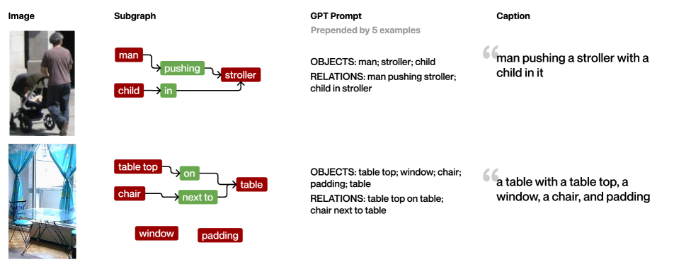
Figure 9: Examples of image-text pairs we generate for our productivity evaluation. The image is the union of the objects bounding boxes in the subgraphs. We also showcase the GPT-3 prompt associated with the subgraph and their corresponding generated ground-truth captions.

For examples of complexity $n=4$, we found that stringing together a simple templated prompt was sufficient to produce fluent captions. This was done by prepending attributes in front of objects and stringing together subjects, relations, and objects in the correct order. For example, a subgraph containing boy=(tall,blue); grass=(green); (boy, on, grass) would be templated as tall and blue boy on green grass. Any disconnected atoms are appended with the prefix “and a.”

Data verification.

Table 4: Productivity ground truth captions’ faithfulness to their paired images, split by caption complexity. Overall, the generated captions’ faithfulness is stable and consistently high across different complexities.

Complexity	Avg faithfulness
$n=7$	$88.7\pm 10.8$
$n=8$	$85.7\pm 7.0$
$n=9$	$90.0\pm 6.0$
$n=10$	$87.7\pm 9.3$
$n=11$	$88.1\pm 7.8$
$n=12$	$89.1\pm 2.9$

We manually verify the accuracy of our produced productivity dataset. We provide a breakdown of annotators’ scores for GPT-3 caption faithfulness across complex subgraphs with $n\geq 7$ in Table 4. We see that scores are consistently high for ground-truth captions across complexities.

A.4 Hard negative generation details

We provide additional detail for the procedure of generating a hard negative of types HN-Swap and HN-Neg. Suppose throughout that for a given image and its annotated scene graph $G$, we seek to generate a hard negative caption for caption $t$ associated with the subgraph $S\subseteq G$.

HN-Swap

The following pairs of atoms could be swapped to create a hard negative for $S$:

• The subject $A_{o}$ and object $A_{o}^{\prime}$ of a relationship compound $C_{oro}\in S$.

• Two attributes $A_{a}$ and $A_{a}^{\prime}$ attached to distinct objects $A_{o}$, $A_{o}^{\prime}$, such that one attribute is not present for the other object in $G$ and vice versa. ($(A_{a},A_{o}^{\prime})\not\in G$ and $(A_{a}^{\prime},A_{o})\not\in G$).

• Two objects $A_{o}$, $A_{o}^{\prime}$ not connected by a relationship such that their swapping within $G$ does not create an identical graph.

Additionally, some swap hard negatives generated are permutations rather than a swapped pair:

• One attribute $A_{a}$ can be transferred from one object $A_{o}$ to another object $A_{o}^{\prime}$, so long as that attribute doesn’t apply to the new object ($(A_{a},A_{o}^{\prime})\notin G$).

• For low complexities ($n=4$), any permutation of atoms of the same type are allowed. For example: (“There is a dog on the bed and also a nightstand" $\rightarrow$ “There is a nightstand on the dog and also a bed")

HN-Neg

We verify with $G$ to ensure that negating an atom results in an incorrect caption. If an attribute $A_{a}$ connected with $A_{o}$ is negated, we ensure that there does not exist an object of $A_{o}^{\prime}$ that doesn’t have an attribute $A_{a}$ but shares all the other attributes of $A_{o}$. For example, if we negate “black" in “Black dog on a building", we ensure there doesn’t exist another dog on the building that isn’t black. Similar checks are performed for negating relationships and objects. When a relationship $A_{r}$ connecting $A_{o}$ and $A_{o}^{\prime}$ is negated, there cannot exist another identical subject and object pair connected by a different relationship $A_{r}^{\prime}$. When an object is negated, there cannot exist any other object with the same attributes and relationships.

A.5 Test dataset sizes, examples, and additional verification

Table 5: We report the ground truth caption counts in ${\mathcal{D}_{test}^{raw}}$ and hard negative counts in $\mathcal{D}_{test}^{HN}$s for systematicity and productivity, separated by hard negative type and split.

Systematicity					Productivity
Split	Ground Truth	HN-Atom	HN-Comp		Split	Ground Truth	HN-Atom	HN-Swap	HN-Neg
CC-12M SC	262,541	104,024	156,036		$n=4$	1,508	6,290	135	2,510
CC-12M UC	113,659	14,348	21,522		$n=5$	1,734	7,270	180	3,425
CC-12M UA	9,577	-	-		$n=6$	1,905	9,025	1,310	6,565
YFCC SC	194,502	75,948	113,922		$n=7$	2,171	10,410	2,525	7,845
YFCC UC	172,469	39,204	58,806		$n=8$	2,247	11,205	4,955	10,210
YFCC UA	18,806	-	-		$n=9$	1,969	9,485	4,420	8,310
LAION SC	170,253	62,884	94,326		$n=10$	2,246	11,325	6,465	10,460
LAION UC	201,595	49,604	74,406		$n=11$	1,895	8,620	5,380	7,925
LAION UA	1,855	-	-		$n=12$	1,878	10,005	7,890	9,710

Table 6: We summarize the retrieval set sizes for both $\mathcal{D}_{test}^{HN}$ and $\mathcal{D}_{test}^{Raw}$ in our systematicity and productivity evaluation.

Retrieval set size	$\mathcal{D}_{test}^{HN}$			$\mathcal{D}_{test}^{RAW}$
Systematicity	HN-Atom	HN-Comp		—
	5	7		1,855
Productivity	HN-Atom	HN-Swap	HN-Neg	—
	6	6	6	1,508

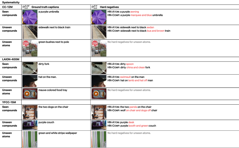
Figure 10: A sample of image-caption pairs in the systematicity retrieval sets. One ground truth caption is shown for each split of each training dataset, each of which lie in both $\mathcal{D}_{test}^{RAW}$ and $\mathcal{D}_{test}^{HN}$. Additionally, one example of each hard negative type is shown for each ground truth caption.

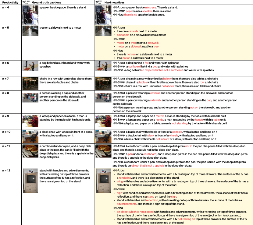
Figure 11: A sample of image-caption pairs in the productivity retrieval sets. One ground truth (GT) caption is shown for each complexity $n$. These GT captions lie in both $\mathcal{D}_{test}^{RAW}$ and $\mathcal{D}_{test}^{HN}$. One example of each hard negative type is shown for each GT caption. For two highlighted example captions ($n=5,12$), we show 2 hard negatives per type for comprehensiveness.

Table 5 expands on Table 1 from the main paper to provide a breakdown of the number of image-text pair per hard negative type and, for productivity, for each sentence complexity. We remark that $\mathcal{D}^{RAW}_{test}$, which contains only image-ground-truth caption pairs, is a superset of the ground-truth captions in $\mathcal{D}^{HN}_{test}$. This is because, for some ground truth captions in $\mathcal{D}^{RAW}_{test}$, a sufficient number of hard negatives to perform retrieval in $\mathcal{D}^{HN}_{test}$ could not be generated. Additionally, due to the prevalence of rare atoms, we could only generate valid hard negatives for very few captions in the UA split. Therefore, we omit the evaluation on the UA split with hard negatives and focus on the analysis of results between the SC and UC split, which is more interesting as models have seen all the atoms in both splits. Table 6 summarizes the text retrieval set size of each image query for both $\mathcal{D}_{test}^{raw}$ and $\mathcal{D}_{test}^{HN}$ in our systematicity and productivity evaluation. Figures 10 and 11 present examples of ground truth captions and hard negative captions in our test datasets for systematicity and productivity, respectively.

We provide a breakdown of annotators’ scores for the accuracy of productivity hard negatives in Table 7. A hard negative caption is accurate if it contains incorrect facts about the image. We find that the accuracy and pairwise agreement of the HN-Atom is the highest and much higher than those of HN-Swap and HN-Neg.

Table 7: Accuracy of our generated hard negatives for productivity, split by type, in our data verification. While HN-Atom atoms receive strong human evaluation scores, we find that HN-Swap and HN-Neg negatives are noisier.

Type	Acc. mean $\pm$ std	Pairwise agreement
HN-Atom	$91.6\pm 4.2$	83.1
HN-Swap	$70.1\pm 9.1$	58.5
HN-Neg	$72.4\pm 0.0$	59.5

A.6 Systematicity hard negative dataset details

Table 8: We summarize the unique atom and compound counts in the SC and UC split of the systematicity hard negative set.

	SC		UC
Train dataset	Atom (seen)	Comp (seen)	Atom (seen)	Comp (unseen)
CC12M	3,348	26,006	946	3,587
YFCC	3,173	18,987	1,405	9,801
LAION	2,968	12,401	1,951	15,721

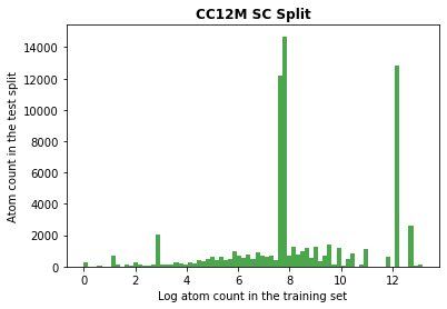
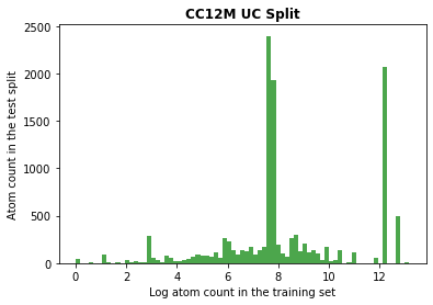
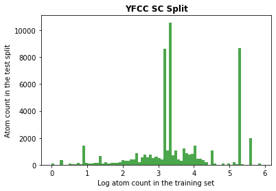
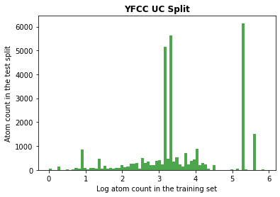
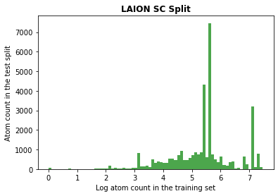
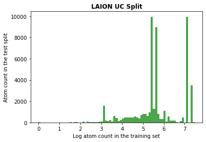
Figure 12: We plot the atom count in training vs. in the systematicity hard negative test set. We observe that the atoms in the SC and UC test splits have similar counts in the training dataset.

Table 8 summarizes the number of unique atoms and compounds in the SC and UC split of the systematicity hard negative set. Additionally, we plot the atom count in the systematicity test set vs. the training set (on a log scale). As shown in Figure 12, we see that the atom count in the training set is always on the same scale across both splits for the same training dataset (x-axis in each row). We further observe that the atom distributions are similar in the SC and UC splits. These suggest that the atoms appearing in the UC split are not substantially rarer or more difficult than the ones in the SC split.

Appendix B Additional evaluation results

B.1 Full retrieval results on hard negative datasets

Table 9: Systematicity HN-Atom + HN-Comp Dataset Analysis. We report Recall@1,3,5 and Avg R@K results for all models on the $D_{test}^{HN}$ hard-negative datasets with both HN-Atom + HN-Comp. Model performance decreases from the Seen all compounds (SC) to the Unseen Compounds (UC) split, particularly for LAION-400M models.

	Training dataset	Model	R@1		R@3		Avg R@K
			SC	UC	SC	UC	SC	UC
		Random	9.09	9.09	27.27	27.27	18.18	18.18
Image-to-text	CC12M	RN50	23.26	19.96	62.44	59.52	42.85	39.74
	YFCC15M	RN50	23.38	20.08	60.09	56.61	41.74	38.34
		RN101	22.74	20.50	59.15	57.59	40.94	39.04
	LAION400M	ViT-B-32	34.28	28.00	70.74	68.74	52.51	48.37
		ViT-B-16	37.01	30.81	73.92	72.85	55.46	51.83
		ViT-B-16+240	37.32	32.26	75.03	73.46	56.17	52.86
		ViT-L-14	39.44	33.81	74.31	73.47	56.87	53.64

Table 10: Systematicity HN-Atom Dataset Analysis. We report Recall@1,3 and Avg R@K results for all models on the $D_{test}^{HN}$ subset with HN-Atom. Model performance decreases from the Seen Compounds (SC) to the Unseen Compounds (UC) split, particularly for LAION-400M models.

	Training dataset	Model	R@1		R@3		Avg R@K
			SC	UC	SC	UC	SC	UC
		Random	20.00	20.00	60.00	60.00	40.00	40.00
Image-to-text	CC12M	RN50	39.26	34.88	88.81	88.10	64.04	61.49
	YFCC15M	RN50	43.35	39.50	90.55	90.07	66.95	64.78
		RN101	43.26	39.85	90.33	90.30	66.79	65.08
	LAION400M	ViT-B-32	55.32	42.75	93.38	91.92	74.35	67.34
		ViT-B-16	57.18	44.93	94.01	92.95	75.59	68.94
		ViT-B-16+240	57.95	46.53	94.36	93.40	76.16	69.97
		ViT-L-14	59.11	47.86	94.39	93.66	76.75	70.76

Table 11: Systematicity HN-COMP Dataset Analysis. We report Recall@1,3 and Avg R@K results for all models on the $D_{test}^{HN}$ subset with HN-COMP. We observe little to no difference in performance between the SC and UC split.

	Training dataset	Model	R@1		R@3		Avg R@K
			SC	UC	SC	UC	SC	UC
		Random	14.29	14.29	42.86	42.86	28.57	28.57
Image-to-text	CC12M	RN50	48.02	45.27	80.24	79.59	64.13	62.43
	YFCC15M	RN50	42.07	39.83	75.06	73.66	58.56	56.74
		RN101	40.72	39.56	74.71	74.16	57.72	56.86
	LAION400M	ViT-B-32	52.29	54.80	82.40	83.25	67.35	69.02
		ViT-B-16	56.00	59.00	84.64	86.24	70.32	72.62
		ViT-B-16+240	56.57	60.19	85.28	85.69	70.92	72.94
		ViT-L-14	57.10	60.78	84.17	85.69	70.64	73.24

Systematicity

We additionally include the full retrieval results on $\mathcal{D}_{test}^{HN}$ with both HN-Atom and HN-Comp, HN-Atom only and HN-Comp only in Tables 9, 10 and 11. We note that as we relax the metric from R@1 to R@3, the difference between models’ performance in the SC and UC split decreases.

Productivity

Table 12: Productivity HN-Atom Dataset Analysis. We report mean Recall@1 results for all models across all complexities. We find that models’ Recall@1 values decrease as caption complexity increases.

	Training dataset	Model	4	5	6	7	8	9	10	11	12
		Random	16.67	16.67	16.67	16.67	16.67	16.67	16.67	16.67	16.67
Image-to-text	CC-12M	RN50	19.71	21.46	16.40	18.35	15.31	14.92	13.38	15.26	12.04
	YFCC-15M	RN50	21.30	23.31	19.94	18.11	15.62	16.03	14.97	15.14	12.89
		RN101	22.66	22.21	18.17	18.44	15.22	16.34	15.85	17.34	13.04
	LAION-400M	ViT-B-32	23.21	21.25	19.06	18.59	16.15	13.92	15.76	15.49	12.84
		ViT-B-16	23.13	22.83	19.89	21.09	18.65	15.92	16.42	17.00	13.39
		ViT-B-16+240	29.73	23.31	21.72	21.81	18.38	18.08	17.62	18.39	14.89
		ViT-L-14	28.54	25.10	21.55	24.06	19.81	18.61	17.88	18.68	15.44
		CyCLIP RN50	18.20	15.13	15.24	14.46	11.91	11.12	11.70	11.95	8.35
		FLAVA	29.17	16.23	14.13	15.08	14.46	14.55	14.88	15.72	14.79
		ALBEF	38.71	32.94	27.87	27.76	26.51	25.94	25.92	27.03	24.34
	CLIP’s dataset	RN50	26.79	26.41	21.83	21.09	18.38	19.40	17.40	19.14	15.49
		RN101	28.46	26.34	22.22	22.33	18.56	19.14	19.16	18.56	17.94
		ViT-B-32	28.70	23.31	21.33	19.79	18.61	18.13	17.66	18.10	16.69
		ViT-B-16	30.68	26.41	23.93	23.15	19.19	19.19	18.76	20.19	16.44
		ViT-L-14	31.00	28.47	22.71	22.48	19.01	21.09	18.01	19.14	18.24

Table 13: Productivity HN-Swap Dataset Analysis. We report mean Recall@1 results for all models across all complexities. We find that models’ Recall@1 values are near or even below random chance across all complexities.

	Training dataset	Model	4	5	6	7	8	9	10	11	12
		Random	16.67	16.67	16.67	16.67	16.67	16.67	16.67	16.67	16.67
Image-to-text	CC-12M	RN50	7.41	19.44	9.92	12.87	12.61	13.12	13.53	14.87	12.93
	YFCC-15M	RN50	11.11	16.67	14.50	15.25	13.32	14.14	10.75	13.48	13.88
		RN101	25.93	30.56	8.40	12.67	11.81	11.76	12.30	13.85	13.69
	LAION-400M	ViT-B-32	25.93	19.44	12.98	13.86	12.31	14.37	11.60	12.08	14.13
		ViT-B-16	14.81	22.22	10.31	14.85	12.31	14.03	13.77	14.87	13.50
		ViT-B-16+240	22.22	22.22	14.12	15.05	14.13	14.48	13.69	18.31	15.91
		ViT-L-14	14.81	22.22	12.60	14.06	12.92	15.61	15.00	17.84	16.79
		CyCLIP RN50	11.11	5.56	11.07	14.46	11.81	12.56	13.23	13.75	11.79
		FLAVA	7.41	19.44	9.16	10.50	9.69	11.65	10.44	12.36	16.22
		ALBEF	25.93	13.89	17.56	20.00	21.19	19.80	20.42	22.12	22.43
	CLIP’s dataset	RN50	22.22	19.44	19.47	20.20	17.66	17.99	17.71	18.49	18.12
		RN101	29.63	25.00	16.79	17.62	17.15	15.38	17.40	19.61	18.06
		ViT-B-32	25.93	22.22	22.90	15.64	15.14	16.63	16.24	20.91	18.95
		ViT-B-16	33.33	22.22	20.99	18.42	17.86	16.40	15.78	19.42	16.79
		ViT-L-14	11.11	13.89	19.08	16.83	17.05	16.86	16.01	18.49	18.06

Table 14: Productivity HN-Neg Dataset Analysis. We report mean Recall@1 results for all models across all complexities. We find that models’ Recall@1 values either stay near random chance or decrease as caption complexity increases except for some of OpenAI’s CLIP models.

	Training dataset	Model	4	5	6	7	8	9	10	11	12
		Random	16.67	16.67	16.67	16.67	16.67	16.67	16.67	16.67	16.67
Image-to-text	CC-12M	RN50	15.13	19.28	18.41	23.59	20.94	20.83	21.95	20.90	18.34
	YFCC-15M	RN50	8.32	10.29	12.18	12.64	12.30	12.23	12.65	13.49	12.96
		RN101	8.56	9.30	10.96	10.35	11.41	10.36	9.88	11.08	10.25
	LAION-400M	ViT-B-32	23.53	18.75	18.08	21.01	20.50	21.88	21.32	20.78	21.36
		ViT-B-16	24.80	26.91	23.47	23.89	25.67	25.88	24.59	25.54	26.98
		ViT-B-16+240	23.53	28.20	26.36	29.12	28.83	27.03	28.30	30.30	27.49
		ViT-L-14	30.35	29.04	26.14	29.92	28.48	27.41	28.70	30.72	29.60
		CyCLIP RN50	16.24	12.65	15.35	14.39	13.19	12.77	13.23	12.77	13.27
		FLAVA	16.16	13.72	16.52	12.29	11.54	14.42	20.25	16.81	12.86
		ALBEF	75.83	45.12	43.55	44.05	47.28	48.19	46.45	47.71	40.05
	CLIP’s dataset	RN50	14.10	34.83	37.10	41.76	41.18	40.90	39.61	40.06	31.41
		RN101	8.72	12.88	15.57	14.73	15.91	18.20	17.34	20.66	25.83
		ViT-B-32	15.85	30.56	34.09	35.99	38.99	40.13	39.87	41.33	38.94
		ViT-B-16	7.13	26.22	28.64	32.11	33.16	31.41	34.29	36.51	31.56
		ViT-L-14	13.79	26.91	26.36	23.05	22.37	24.07	24.05	27.17	24.92

We report the full retrieval results on productivity $\mathcal{D}_{test}^{HN}$ sets in Tables 12, 14 and 13.

B.2 Retrieval results on raw datasets

Table 15: Systematicity Raw Dataset Analysis. We report mean Recall@1 results for all models across k-fold evaluations. Model performance consistently decreases from Seen all Compounds (SC) to Unseen Compounds (UC) and from Unseen Compounds to Unseen Atoms (UA) splits, particularly for LAION-400M models.

	Training dataset	Model	SC	UC	UA
		Random	$0.05\pm 0.00$	$0.05\pm 0.00$	$0.05\pm 0.00$
Image-to-text	CC-12M	RN50	$19.92\pm 0.94$	$17.82\pm 0.99$	$15.02\pm 0.85$
	YFCC-15M	RN50	$16.30\pm 0.70$	$14.57\pm 0.69$	$12.80\pm 0.90$
		RN101	$17.10\pm 0.90$	$15.58\pm 1.04$	$13.62\pm 0.84$
	LAION-400M	ViT-B-16	$35.61\pm 0.92$	$30.04\pm 1.42$	$25.88\pm 0.00$
		ViT-B-16+240	$36.80\pm 0.90$	$31.10\pm 1.37$	$26.25\pm 0.00$
		ViT-B-32	$33.86\pm 0.97$	$29.00\pm 1.40$	$23.99\pm 0.00$
		ViT-L-14	$38.24\pm 0.70$	$32.70\pm 1.30$	$26.42\pm 0.00$
Text-to-image	CC-12M	RN50	$20.85\pm 0.98$	$18.15\pm 0.84$	$15.46\pm 1.10$
	YFCC-15M	RN50	$15.60\pm 0.79$	$14.05\pm 0.84$	$12.17\pm 0.64$
		RN101	$16.11\pm 0.84$	$14.47\pm 0.87$	$12.54\pm 0.66$
	LAION-400M	ViT-B-16	$35.74\pm 0.76$	$29.58\pm 1.39$	$23.29\pm 0.00$
		ViT-B-16+240	$37.25\pm 0.97$	$30.57\pm 1.33$	$24.26\pm 0.00$
		ViT-B-32	$33.66\pm 1.03$	$29.00\pm 1.40$	$22.10\pm 0.00$
		ViT-L-14	$38.69\pm 0.86$	$32.00\pm 0.90$	$25.61\pm 0.00$

Table 16: Productivity Raw Dataset Analysis. We report mean Recall@1 results for all models across all complexities. We find that models’ Recall@1 increases as the caption complexity increases.

	Training dataset	Model	4	5	6	7	8	9	10	11	12
		Random	0.06	0.06	0.06	0.06	0.06	0.06	0.06	0.06	0.06
Image-to-text	CC-12M	RN50	13.19	14.23	16.20	19.02	21.17	19.26	22.70	24.29	25.77
	YFCC-15M	RN50	9.08	10.92	12.09	14.23	14.17	15.40	14.54	16.75	19.02
		RN101	11.10	11.47	11.90	14.60	15.34	16.50	16.99	18.90	20.67
	LAION-400M	ViT-B-16	20.80	20.00	25.89	27.30	29.63	29.02	30.31	34.11	37.36
		ViT-B-16+240	22.39	21.53	26.93	28.10	30.61	30.18	32.88	36.50	38.83
		ViT-B-32	20.49	20.37	23.50	26.93	29.20	28.22	29.94	32.58	35.40
		ViT-L-14	22.09	23.07	27.67	29.69	33.13	31.04	35.09	37.12	40.25
Text-to-image	CC-12M	RN50	12.52	15.03	15.52	17.85	17.30	19.75	21.66	22.52	25.58
	YFCC-15M	RN50	8.04	9.82	9.82	12.15	12.94	13.62	13.37	14.97	15.15
		RN101	9.39	11.10	11.10	13.31	13.74	15.03	14.48	16.07	18.40
	LAION-400M	ViT-B-16	18.16	19.26	23.62	24.85	27.85	27.79	28.77	31.53	33.93
		ViT-B-16+240	18.96	20.67	25.46	26.13	28.83	29.02	31.41	32.88	37.24
		ViT-B-32	17.55	18.65	22.21	23.50	26.20	26.13	27.36	28.83	32.21
		ViT-L-14	19.88	20.43	24.97	26.63	30.37	30.00	32.76	34.42	36.99

In addition to $\mathcal{D}^{HN}_{test}$ retrieval experiments, we perform retrieval experiments with $\mathcal{D}^{RAW}_{test}$.

We perform both image-to-text and text-to-image retrieval within splits of $\mathcal{D}_{test}^{RAW}$. Each retrieval task is between one image and every caption in the split, or vice versa. We report the mean and standard deviation of Recall@1 across K-fold retrievals (where $K=\min(20,\lfloor\frac{|\mathcal{D}^{RAW}_{test}|}{N}\rfloor)$, and $N=\min\{|SC|,|UC|,|UA|\}=1855$ for systematicity and $N=\min_{n\in\{4\ldots 12\}}|\mathcal{D}_{test}^{RAW,n}|=1508$ for productivity), as the data size varies across compositional splits and complexities.

Systematicity

We present the systematicity retrieval results on $\mathcal{D}_{test}^{raw}$ in Table 15, where each retrieval set for an image consists of the captions of the other images. We continue to observe a monotonic decrease in performance when compounds are unseen. Additionally, we continue to observe a drop in performance for larger training datasets. In particular, we see a similar drop in performance for LAION-trained models across both the image-to-text and text-to-image tasks. We also observe larger drops on LAION-trained models than for $\mathcal{D}_{test}^{HN}$ when moving across the $\textsc{SC}\to\textsc{UC}$, and across $\textsc{UC}\to\textsc{UA}$ splits, with LAION models dropping as much as $13\%$ for ViT-L/14.

Productivity

We additionally present the productivity retrieval results on $\mathcal{D}_{test}^{raw}$ in Table 16. We observe that models’ Recall@1 generally increases as the caption complexity increases. We hypothesize that models’ low performance in the low-complexity subset is caused by false negatives in the original dataset: since the captions are simple and likely true for multiple images, there are multiple false negatives in the retrieval set, making these numbers unreliable. As the captions become more complex, however, the chance of such false negatives is lower. This means there are more true negatives in the higher-complexity subsets, making retrieval easier for these models.

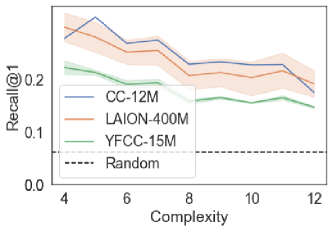
Figure 13: Productivity Analysis on Hard Negatives of All Types. We plot models’ Recall@1 on the overall hard negatives retrieval set against complexity, where each retrieval set contains hard negatives of all types. We find that models’ ability to correctly retrieve the ground-truth caption drops as complexity increases.

B.3 Retrieval results with all hard negatives at once

Productivity

We present models’ retrieval performances over the whole productivity $\mathcal{D}_{test}^{HN}$ dataset, where each retrieval set contains one ground truth caption and fifteen hard negatives, five for each of the three types HN-Atom, HN-Swap and HN-Neg. We find in Figure 13 that models’ Recall@1 performance decreases with complexity, which aligns with the findings on the separate retrieval sets for HN-Atom, HN-Swap and HN-Neg.

Table 17: Systematicity Qualitative Analysis. We present examples where LAION-400M trained ViT-B-16 and ViT-L-14 both perform well on the Seen Compounds (SC) split, and where ViT-B-16 performs poorly on the Unseen Compounds (UC) split.

			ViT-B-16		ViT-L-14
	Image	GT caption	R@1	Top 3 captions	R@1	Top 3 captions
SC		purple couch	1	purple couch purple altar and brown couch purple commode and red couch	1	purple couch purple altar and brown couch purple desk and brown couch
		a white parked car	1	a white parked car a green parked car a white bike	1	a white parked car a green parked car a orange parked car
		a fully grown brown horse	1	a fully grown brown horse a fully grown brown mule and red horse a fully grown brown mule and yellow horse	1	a fully grown brown horse a fully grown brown mule and red horse a fully grown brown zebra and blue horse
UC		a cat on the sofa.	0	a cat on the console. a cat on the sofa. cat on counter and cat off sofa	1	a cat on the sofa. a cat on the console. badger on sofa and cat on console
		boat on the water	0	boat on the polish boat on the soda boat on the water	1	boat on the water boat on the lime ship on water and boat on rubber
		plants on a building	0	plants on bob and plants off building plants on a building court on building and plants off building	1	plants on a building park on a building billboard on building and plants off building

B.4 Qualitative analysis on systematicity evaluation

We perform a qualitative analysis to better understand why the LAION-400M trained models ViT-B-16 and ViT-L-14 show a large versus small performance drop from the Seen to Unseen Compounds split respectively. Table 17 presents examples where both ViT-B-16 and ViT-L-14 retrieve the correct caption successfully in the SC split and where VT-B-16 fails in the UC split. Through this analysis, we find that the SC split for LAION-400M trained models is dominated by simple two-atom examples such as “purple couch”. The UC split, however, contains more complex examples that involve relationships such as “curtains on the window”. In particular, we find that the ViT-B-16 model struggles with the relationship “on” and often retrieves a wrong caption where “on” is replaced with “off” or where the object is replaced with an atomic foil. For example, ViT-B-16 retrieves “plants on bob and plants off building” incorrectly when the groundtruth caption is “plants on a building”. Nevertheless, the rank of the groundtruth caption is often still within the top three. This explains the narrower gap in ViT-B-16’ Recall@3 between Seen Compounds and Unseen Compounds. On the other hand, we see that ViT-L-14 continues to retrieve the correct caption even on the more challenging Unseen Compounds split, suggesting that a larger model size could improve compositional systematicity.

Appendix C Additional Related Work

Evaluating learned representations By analyzing the properties of pretrained representations, our work continues a tradition of research in Computer Vision [49, 71, 58, 57, 90, 19] and Natural Language Processing [70, 36, 86, 92, 26, 66] that probes characteristics of representations themselves rather than their performance on downstream tasks. Instead of learning probes, we use retrieval for zero-shot evaluation in order to avoid scenarios where the learned probe compensates for the characteristics deficient in the original representations [27, 4, 9, 44, 99].

References

- [1] Arjun Akula, Spandana Gella, Yaser Al-Onaizan, Song-Chun Zhu, and Siva Reddy. Words aren’t enough, their order matters: On the robustness of grounding visual referring expressions. In Proceedings of the 58th Annual Meeting of the Association for Computational Linguistics, pages 6555–6565, Online, July 2020. Association for Computational Linguistics.
- [2] Jacob Andreas, Marcus Rohrbach, Trevor Darrell, and Dan Klein. Neural module networks, 2015.
- [3] Dzmitry Bahdanau, Harm de Vries, Timothy J O’Donnell, Shikhar Murty, Philippe Beaudoin, Yoshua Bengio, and Aaron Courville. Closure: Assessing systematic generalization of clevr models. arXiv preprint arXiv:1912.05783, 2019.
- [4] Yonatan Belinkov. Probing classifiers: Promises, shortcomings, and advances. Computational Linguistics, 48(1):207–219, Mar. 2022.
- [5] Ben Bogin, Shivanshu Gupta, Matt Gardner, and Jonathan Berant. COVR: A test-bed for visually grounded compositional generalization with real images. In Proceedings of the 2021 Conference on Empirical Methods in Natural Language Processing, pages 9824–9846, Online and Punta Cana, Dominican Republic, Nov. 2021. Association for Computational Linguistics.
- [6] Rishi Bommasani, Drew A Hudson, Ehsan Adeli, Russ Altman, Simran Arora, Sydney von Arx, Michael S Bernstein, Jeannette Bohg, Antoine Bosselut, Emma Brunskill, et al. On the opportunities and risks of foundation models. arXiv preprint arXiv:2108.07258, 2021.
- [7] Léon Bottou. From machine learning to machine reasoning. Machine learning, 94(2):133–149, 2014.
- [8] Tom Brown, Benjamin Mann, Nick Ryder, Melanie Subbiah, Jared D Kaplan, Prafulla Dhariwal, Arvind Neelakantan, Pranav Shyam, Girish Sastry, Amanda Askell, et al. Language models are few-shot learners. Advances in neural information processing systems, 33:1877–1901, 2020.
- [9] Steven Cao, Victor Sanh, and Alexander M Rush. Low-complexity probing via finding subnetworks. arXiv preprint arXiv:2104.03514, 2021.
- [10] Soravit Changpinyo, Piyush Sharma, Nan Ding, and Radu Soricut. Conceptual 12m: Pushing web-scale image-text pre-training to recognize long-tail visual concepts. In Proceedings of the IEEE/CVF Conference on Computer Vision and Pattern Recognition, pages 3558–3568, 2021.
- [11] Zhenfang Chen, Peng Wang, Lin Ma, Kwan-Yee K. Wong, and Qi Wu. Cops-ref: A new dataset and task on compositional referring expression comprehension, 2020.
- [12] Colin Conwell and Tomer Ullman. Testing relational understanding in text-guided image generation. arXiv preprint arXiv:2208.00005, 2022.
- [13] MJ Cresswell. Logics and languages. 1973.
- [14] Yuchen Cui, Scott Niekum, Abhinav Gupta, Vikash Kumar, and Aravind Rajeswaran. Can foundation models perform zero-shot task specification for robot manipulation? In Roya Firoozi, Negar Mehr, Esen Yel, Rika Antonova, Jeannette Bohg, Mac Schwager, and Mykel Kochenderfer, editors, Proceedings of The 4th Annual Learning for Dynamics and Control Conference, volume 168 of Proceedings of Machine Learning Research, pages 893–905. PMLR, 23–24 Jun 2022.
- [15] Jacob Devlin, Ming-Wei Chang, Kenton Lee, and Kristina Toutanova. Bert: Pre-training of deep bidirectional transformers for language understanding. arXiv preprint arXiv:1810.04805, 2018.
- [16] Alexey Dosovitskiy, Lucas Beyer, Alexander Kolesnikov, Dirk Weissenborn, Xiaohua Zhai, Thomas Unterthiner, Mostafa Dehghani, Matthias Minderer, Georg Heigold, Sylvain Gelly, Jakob Uszkoreit, and Neil Houlsby. An image is worth 16x16 words: Transformers for image recognition at scale. In International Conference on Learning Representations, 2021.
- [17] Jiali Duan, Liqun Chen, Son Tran, Jinyu Yang, Yi Xu, Belinda Zeng, and Trishul Chilimbi. Multi-modal alignment using representation codebook, 2022.
- [18] Sepideh Esmaeilpour, Bing Liu, Eric Robertson, and Lei Shu. Zero-shot out-of-distribution detection based on the pre-trained model clip, 2021.
- [19] Stella Frank, Emanuele Bugliarello, and Desmond Elliott. Vision-and-language or vision-for-language? on cross-modal influence in multimodal transformers. In Proceedings of the 2021 Conference on Empirical Methods in Natural Language Processing, pages 9847–9857, Online and Punta Cana, Dominican Republic, Nov. 2021. Association for Computational Linguistics.
- [20] Mona Gandhi, Mustafa O. Gul, Eva Prakash, Madeleine Grunde-McLaughlin, Ranjay Krishna, and Maneesh Agrawala. Measuring compositional consistency for video question answering. In Proceedings of the IEEE/CVF Conference on Computer Vision and Pattern Recognition, 2022.
- [21] Shashank Goel, Hritik Bansal, Sumit Bhatia, Ryan A. Rossi, Vishwa Vinay, and Aditya Grover. Cyclip: Cyclic contrastive language-image pretraining, 2022.
- [22] Madeleine Grunde-McLaughlin, Ranjay Krishna, and Maneesh Agrawala. Agqa: A benchmark for compositional spatio-temporal reasoning. In Proceedings of the IEEE/CVF Conference on Computer Vision and Pattern Recognition, 2021.
- [23] Kaiming He, Xiangyu Zhang, Shaoqing Ren, and Jian Sun. Deep residual learning for image recognition. In Proceedings of the IEEE conference on computer vision and pattern recognition, pages 770–778, 2016.
- [24] Lisa Anne Hendricks and Aida Nematzadeh. Probing image-language transformers for verb understanding, 2021.
- [25] Jack Hessel, Ari Holtzman, Maxwell Forbes, Ronan Le Bras, and Yejin Choi. CLIPScore: A reference-free evaluation metric for image captioning. In Proceedings of the 2021 Conference on Empirical Methods in Natural Language Processing, pages 7514–7528, Online and Punta Cana, Dominican Republic, Nov. 2021. Association for Computational Linguistics.
- [26] Jack Hessel and Alexandra Schofield. How effective is BERT without word ordering? implications for language understanding and data privacy. In Proceedings of the 59th Annual Meeting of the Association for Computational Linguistics and the 11th International Joint Conference on Natural Language Processing (Volume 2: Short Papers), pages 204–211, Online, Aug. 2021. Association for Computational Linguistics.
- [27] John Hewitt and Percy Liang. Designing and interpreting probes with control tasks. In Proceedings of the 2019 Conference on Empirical Methods in Natural Language Processing and the 9th International Joint Conference on Natural Language Processing (EMNLP-IJCNLP), pages 2733–2743, Hong Kong, China, Nov. 2019. Association for Computational Linguistics.
- [28] Irina Higgins, Nicolas Sonnerat, Loic Matthey, Arka Pal, Christopher P Burgess, Matko Bosnjak, Murray Shanahan, Matthew Botvinick, Demis Hassabis, and Alexander Lerchner. Scan: Learning hierarchical compositional visual concepts. arXiv preprint arXiv:1707.03389, 2017.
- [29] Hexiang Hu, Ishan Misra, and Laurens van der Maaten. Evaluating text-to-image matching using binary image selection (bison), 2019.
- [30] Drew A. Hudson and Christopher D. Manning. Compositional attention networks for machine reasoning, 2018.
- [31] Drew A Hudson and Christopher D Manning. Gqa: A new dataset for real-world visual reasoning and compositional question answering. Conference on Computer Vision and Pattern Recognition (CVPR), 2019.
- [32] Dieuwke Hupkes, Verna Dankers, Mathijs Mul, and Elia Bruni. Compositionality decomposed: How do neural networks generalise? Journal of Artificial Intelligence Research, 67:757–795, 2020.
- [33] Gabriel Ilharco, Mitchell Wortsman, Ross Wightman, Cade Gordon, Nicholas Carlini, Rohan Taori, Achal Dave, Vaishaal Shankar, Hongseok Namkoong, John Miller, Hannaneh Hajishirzi, Ali Farhadi, and Ludwig Schmidt. OpenCLIP, 7 2021.
- [34] Ajay Jain, Matthew Tancik, and Pieter Abbeel. Putting nerf on a diet: Semantically consistent few-shot view synthesis. In Proceedings of the IEEE/CVF International Conference on Computer Vision (ICCV), pages 5885–5894, October 2021.
- [35] Theo MV Janssen and Barbara H Partee. Compositionality. In Handbook of logic and language, pages 417–473. Elsevier, 1997.
- [36] Ganesh Jawahar, Benoît Sagot, and Djamé Seddah. What does BERT learn about the structure of language? In Proceedings of the 57th Annual Meeting of the Association for Computational Linguistics, pages 3651–3657, Florence, Italy, July 2019. Association for Computational Linguistics.
- [37] Jingwei Ji, Ranjay Krishna, Li Fei-Fei, and Juan Carlos Niebles. Action genome: Actions as compositions of spatio-temporal scene graphs. In Proceedings of the IEEE/CVF Conference on Computer Vision and Pattern Recognition, pages 10236–10247, 2020.
- [38] Chao Jia, Yinfei Yang, Ye Xia, Yi-Ting Chen, Zarana Parekh, Hieu Pham, Quoc Le, Yun-Hsuan Sung, Zhen Li, and Tom Duerig. Scaling up visual and vision-language representation learning with noisy text supervision. In International Conference on Machine Learning, pages 4904–4916. PMLR, 2021.
- [39] Justin Johnson, Bharath Hariharan, Laurens van der Maaten, Li Fei-Fei, C. Lawrence Zitnick, and Ross Girshick. Clevr: A diagnostic dataset for compositional language and elementary visual reasoning, 2016.
- [40] Daniel Keysers, Nathanael Schärli, Nathan Scales, Hylke Buisman, Daniel Furrer, Sergii Kashubin, Nikola Momchev, Danila Sinopalnikov, Lukasz Stafiniak, Tibor Tihon, Dmitry Tsarkov, Xiao Wang, Marc van Zee, and Olivier Bousquet. Measuring compositional generalization: A comprehensive method on realistic data. In International Conference on Learning Representations, 2020.
- [41] Ranjay Krishna, Yuke Zhu, Oliver Groth, Justin Johnson, Kenji Hata, Joshua Kravitz, Stephanie Chen, Yannis Kalantidis, Li-Jia Li, David A Shamma, Michael Bernstein, and Li Fei-Fei. Visual genome: Connecting language and vision using crowdsourced dense image annotations. 2016.
- [42] Brenden Lake and Marco Baroni. Generalization without systematicity: On the compositional skills of sequence-to-sequence recurrent networks. In International conference on machine learning, pages 2873–2882. PMLR, 2018.
- [43] Brenden M. Lake, Tomer D. Ullman, Joshua B. Tenenbaum, and Samuel J. Gershman. Building machines that learn and think like people. Behavioral and Brain Sciences, 40:e253, 2017.
- [44] Michael Lepori and R Thomas McCoy. Picking bert’s brain: Probing for linguistic dependencies in contextualized embeddings using representational similarity analysis. In Proceedings of the 28th International Conference on Computational Linguistics, pages 3637–3651, 2020.
- [45] Boyi Li, Kilian Q Weinberger, Serge Belongie, Vladlen Koltun, and Rene Ranftl. Language-driven semantic segmentation. In International Conference on Learning Representations, 2022.
- [46] Dongxu Li, Junnan Li, Hongdong Li, Juan Carlos Niebles, and Steven C.H. Hoi. Align and prompt: Video-and-language pre-training with entity prompts. In 2022 IEEE/CVF Conference on Computer Vision and Pattern Recognition (CVPR), pages 4943–4953, 2022.
- [47] Junnan Li, Dongxu Li, Caiming Xiong, and Steven Hoi. Blip: Bootstrapping language-image pre-training for unified vision-language understanding and generation. In ICML, 2022.
- [48] Junnan Li, Ramprasaath R. Selvaraju, Akhilesh Deepak Gotmare, Shafiq Joty, Caiming Xiong, and Steven Hoi. Align before fuse: Vision and language representation learning with momentum distillation. In A. Beygelzimer, Y. Dauphin, P. Liang, and J. Wortman Vaughan, editors, Advances in Neural Information Processing Systems, 2021.
- [49] Liunian Harold Li, Mark Yatskar, Da Yin, Cho-Jui Hsieh, and Kai-Wei Chang. What does BERT with vision look at? In Proceedings of the 58th Annual Meeting of the Association for Computational Linguistics, pages 5265–5275, Online, July 2020. Association for Computational Linguistics.
- [50] Wei Li, Can Gao, Guocheng Niu, Xinyan Xiao, Hao Liu, Jiachen Liu, Hua Wu, and Haifeng Wang. UNIMO-2: End-to-end unified vision-language grounded learning. In Findings of the Association for Computational Linguistics: ACL 2022, pages 3187–3201, Dublin, Ireland, May 2022. Association for Computational Linguistics.
- [51] Yehao Li, Yingwei Pan, Ting Yao, and Tao Mei. Comprehending and ordering semantics for image captioning. In Proceedings of the IEEE/CVF Conference on Computer Vision and Pattern Recognition, 2022.
- [52] Zhiheng Li, Martin Renqiang Min, Kai Li, and Chenliang Xu. Stylet2i: Toward compositional and high-fidelity text-to-image synthesis. In Proceedings of the IEEE/CVF Conference on Computer Vision and Pattern Recognition (CVPR), 2022.
- [53] Tsung-Yi Lin, Michael Maire, Serge Belongie, James Hays, Pietro Perona, Deva Ramanan, Piotr Dollár, and C Lawrence Zitnick. Microsoft coco: Common objects in context. In European conference on computer vision, pages 740–755. Springer, 2014.
- [54] Xihui Liu, Dong Huk Park, Samaneh Azadi, Gong Zhang, Arman Chopikyan, Yuxiao Hu, Humphrey Shi, Anna Rohrbach, and Trevor Darrell. More control for free! image synthesis with semantic diffusion guidance, 2021.
- [55] Yinhan Liu, Myle Ott, Naman Goyal, Jingfei Du, Mandar Joshi, Danqi Chen, Omer Levy, Mike Lewis, Luke Zettlemoyer, and Veselin Stoyanov. Roberta: A robustly optimized bert pretraining approach. arXiv preprint arXiv:1907.11692, 2019.
- [56] Haoyu Lu, Nanyi Fei, Yuqi Huo, Yizhao Gao, Zhiwu Lu, and Ji-Rong Wen. Cots: Collaborative two-stream vision-language pre-training model for cross-modal retrieval, 2022.
- [57] Joanna Materzynska, Antonio Torralba, and David Bau. Disentangling visual and written concepts in clip, 2022.
- [58] Victor Milewski, Miryam de Lhoneux, and Marie-Francine Moens. Finding structural knowledge in multimodal-BERT. In Proceedings of the 60th Annual Meeting of the Association for Computational Linguistics (Volume 1: Long Papers), pages 5658–5671, Dublin, Ireland, May 2022. Association for Computational Linguistics.
- [59] George A Miller. Wordnet: a lexical database for english. Communications of the ACM, 38(11):39–41, 1995.
- [60] Medhini Narasimhan, Anna Rohrbach, and Trevor Darrell. Clip-it! language-guided video summarization. 2021.
- [61] Letitia Parcalabescu, Michele Cafagna, Lilitta Muradjan, Anette Frank, Iacer Calixto, and Albert Gatt. VALSE: A task-independent benchmark for vision and language models centered on linguistic phenomena. In Proceedings of the 60th Annual Meeting of the Association for Computational Linguistics (Volume 1: Long Papers), pages 8253–8280, Dublin, Ireland, May 2022. Association for Computational Linguistics.
- [62] Dong Huk Park, Samaneh Azadi, Xihui Liu, Trevor Darrell, and Anna Rohrbach. Benchmark for compositional text-to-image synthesis. In Thirty-fifth Conference on Neural Information Processing Systems Datasets and Benchmarks Track (Round 1), 2021.
- [63] Jae Sung Park, Sheng Shen, Ali Farhadi, Trevor Darrell, Yejin Choi, and Anna Rohrbach. Exposing the limits of video-text models through contrast sets. In Proceedings of the 2022 Conference of the North American Chapter of the Association for Computational Linguistics: Human Language Technologies, pages 3574–3586, Seattle, United States, July 2022. Association for Computational Linguistics.
- [64] Or Patashnik, Zongze Wu, Eli Shechtman, Daniel Cohen-Or, and Dani Lischinski. Styleclip: Text-driven manipulation of stylegan imagery. In Proceedings of the IEEE/CVF International Conference on Computer Vision (ICCV), pages 2085–2094, October 2021.
- [65] Suzanne Petryk, Lisa Dunlap, Keyan Nasseri, Joseph Gonzalez, Trevor Darrell, and Anna Rohrbach. On guiding visual attention with language specification. In 2022 IEEE/CVF Conference on Computer Vision and Pattern Recognition (CVPR), pages 18071–18081, 2022.
- [66] Thang Pham, Trung Bui, Long Mai, and Anh Nguyen. Out of order: How important is the sequential order of words in a sentence in natural language understanding tasks? In Findings of the Association for Computational Linguistics: ACL-IJCNLP 2021, pages 1145–1160, Online, Aug. 2021. Association for Computational Linguistics.
- [67] Alec Radford, Jong Wook Kim, Chris Hallacy, Aditya Ramesh, Gabriel Goh, Sandhini Agarwal, Girish Sastry, Amanda Askell, Pamela Mishkin, Jack Clark, et al. Learning transferable visual models from natural language supervision. In International Conference on Machine Learning, pages 8748–8763. PMLR, 2021.
- [68] Aditya Ramesh, Prafulla Dhariwal, Alex Nichol, Casey Chu, and Mark Chen. Hierarchical text-conditional image generation with clip latents. arXiv preprint arXiv:2204.06125, 2022.
- [69] Yongming Rao, Wenliang Zhao, Guangyi Chen, Yansong Tang, Zheng Zhu, Guan Huang, Jie Zhou, and Jiwen Lu. Denseclip: Language-guided dense prediction with context-aware prompting. In Proceedings of the IEEE Conference on Computer Vision and Pattern Recognition (CVPR), 2022.
- [70] Anna Rogers, Olga Kovaleva, and Anna Rumshisky. A primer in BERTology: What we know about how BERT works. Transactions of the Association for Computational Linguistics, 8:842–866, 2020.
- [71] Philipp J. Rösch and Jindřich Libovický. Probing the role of positional information in vision-language models. In Findings of the Association for Computational Linguistics: NAACL 2022, pages 1031–1041, Seattle, United States, July 2022. Association for Computational Linguistics.
- [72] Laura Ruis, Jacob Andreas, Marco Baroni, Diane Bouchacourt, and Brenden M. Lake. A benchmark for systematic generalization in grounded language understanding. In Proceedings of the 34th International Conference on Neural Information Processing Systems, NIPS’20, Red Hook, NY, USA, 2020. Curran Associates Inc.
- [73] Chitwan Saharia, William Chan, Saurabh Saxena, Lala Li, Jay Whang, Emily Denton, Seyed Kamyar Seyed Ghasemipour, Burcu Karagol Ayan, S Sara Mahdavi, Rapha Gontijo Lopes, et al. Photorealistic text-to-image diffusion models with deep language understanding. arXiv preprint arXiv:2205.11487, 2022.
- [74] Maarten Sap, Ronan Le Bras, Emily Allaway, Chandra Bhagavatula, Nicholas Lourie, Hannah Rashkin, Brendan Roof, Noah A. Smith, and Yejin Choi. ATOMIC: an atlas of machine commonsense for if-then reasoning. CoRR, abs/1811.00146, 2018.
- [75] Christoph Schuhmann, Richard Vencu, Romain Beaumont, Robert Kaczmarczyk, Clayton Mullis, Aarush Katta, Theo Coombes, Jenia Jitsev, and Aran Komatsuzaki. Laion-400m: Open dataset of clip-filtered 400 million image-text pairs. arXiv preprint arXiv:2111.02114, 2021.
- [76] Sebastian Schuster, Ranjay Krishna, Angel Chang, Li Fei-Fei, and Christopher D Manning. Generating semantically precise scene graphs from textual descriptions for improved image retrieval. In Proceedings of the fourth workshop on vision and language, pages 70–80, 2015.
- [77] Piyush Sharma, Nan Ding, Sebastian Goodman, and Radu Soricut. Conceptual captions: A cleaned, hypernymed, image alt-text dataset for automatic image captioning. In Proceedings of ACL, 2018.
- [78] Ravi Shekhar, Sandro Pezzelle, Yauhen Klimovich, Aurélie Herbelot, Moin Nabi, Enver Sangineto, and Raffaella Bernardi. FOIL it! find one mismatch between image and language caption. In Proceedings of the 55th Annual Meeting of the Association for Computational Linguistics (Volume 1: Long Papers), pages 255–265, Vancouver, Canada, July 2017. Association for Computational Linguistics.
- [79] Sheng Shen, Liunian Harold Li, Hao Tan, Mohit Bansal, Anna Rohrbach, Kai-Wei Chang, Zhewei Yao, and Kurt Keutzer. How much can CLIP benefit vision-and-language tasks? In International Conference on Learning Representations, 2022.
- [80] Hengcan Shi, Munawar Hayat, Yicheng Wu, and Jianfei Cai. Proposalclip: Unsupervised open-category object proposal generation via exploiting clip cues, 2022.
- [81] Mohit Shridhar, Lucas Manuelli, and Dieter Fox. Cliport: What and where pathways for robotic manipulation. In Proceedings of the 5th Conference on Robot Learning (CoRL), 2021.
- [82] Amanpreet Singh, Ronghang Hu, Vedanuj Goswami, Guillaume Couairon, Wojciech Galuba, Marcus Rohrbach, and Douwe Kiela. Flava: A foundational language and vision alignment model, 2021.
- [83] Kihyuk Sohn. Improved deep metric learning with multi-class n-pair loss objective. Advances in neural information processing systems, 29, 2016.
- [84] Sanjay Subramanian, Will Merrill, Trevor Darrell, Matt Gardner, Sameer Singh, and Anna Rohrbach. Reclip: A strong zero-shot baseline for referring expression comprehension. arXiv preprint arXiv:2204.05991, 2022.
- [85] Alane Suhr, Stephanie Zhou, Ally Zhang, Iris Zhang, Huajun Bai, and Yoav Artzi. A corpus for reasoning about natural language grounded in photographs. In Proceedings of the 57th Annual Meeting of the Association for Computational Linguistics, pages 6418–6428, Florence, Italy, July 2019. Association for Computational Linguistics.
- [86] Ian Tenney, Dipanjan Das, and Ellie Pavlick. BERT rediscovers the classical NLP pipeline. In Proceedings of the 57th Annual Meeting of the Association for Computational Linguistics, pages 4593–4601, Florence, Italy, July 2019. Association for Computational Linguistics.
- [87] Yoad Tewel, Yoav Shalev, Idan Schwartz, and Lior Wolf. Zero-shot image-to-text generation for visual-semantic arithmetic. arXiv preprint arXiv:2111.14447, 2021.
- [88] Bart Thomee, David A Shamma, Gerald Friedland, Benjamin Elizalde, Karl Ni, Douglas Poland, Damian Borth, and Li-Jia Li. Yfcc100m: The new data in multimedia research. Communications of the ACM, 59(2):64–73, 2016.
- [89] Tristan Thrush, Ryan Jiang, Max Bartolo, Amanpreet Singh, Adina Williams, Douwe Kiela, and Candace Ross. Winoground: Probing vision and language models for visio-linguistic compositionality. In Proceedings of the IEEE/CVF Conference on Computer Vision and Pattern Recognition, pages 5238–5248, 2022.
- [90] Tristan Thrush, Ryan Jiang, Max Bartolo, Amanpreet Singh, Adina Williams, Douwe Kiela, and Candace Ross. Winoground: Probing vision and language models for visio-linguistic compositionality, 2022.
- [91] Mengmeng Wang, Jiazheng Xing, and Yong Liu. Actionclip: A new paradigm for video action recognition, 2021.
- [92] Albert Webson and Ellie Pavlick. Do prompt-based models really understand the meaning of their prompts? In Proceedings of the 2022 Conference of the North American Chapter of the Association for Computational Linguistics: Human Language Technologies, pages 2300–2344, Seattle, United States, July 2022. Association for Computational Linguistics.
- [93] Hao Wu, Jiayuan Mao, Yufeng Zhang, Yuning Jiang, Lei Li, Weiwei Sun, and Wei-Ying Ma. Unified visual-semantic embeddings: Bridging vision and language with structured meaning representations. In Proceedings of the IEEE/CVF Conference on Computer Vision and Pattern Recognition, pages 6609–6618, 2019.
- [94] Hu Xu, Gargi Ghosh, Po-Yao Huang, Dmytro Okhonko, Armen Aghajanyan, Florian Metze, Luke Zettlemoyer, and Christoph Feichtenhofer. VideoCLIP: Contrastive pre-training for zero-shot video-text understanding. In Proceedings of the 2021 Conference on Empirical Methods in Natural Language Processing, pages 6787–6800, Online and Punta Cana, Dominican Republic, Nov. 2021. Association for Computational Linguistics.
- [95] Zipeng Xu, Tianwei Lin, Hao Tang, Fu Li, Dongliang He, Nicu Sebe, Radu Timofte, Luc Van Gool, and Errui Ding. Predict, prevent, and evaluate: Disentangled text-driven image manipulation empowered by pre-trained vision-language model. arXiv preprint arXiv:2111.13333, 2021.
- [96] Jinyu Yang, Jiali Duan, Son Tran, Yi Xu, Sampath Chanda, Liqun Chen, Belinda Zeng, Trishul Chilimbi, and Junzhou Huang. Vision-language pre-training with triple contrastive learning. 2022.
- [97] Jiahui Yu, Zirui Wang, Vijay Vasudevan, Legg Yeung, Mojtaba Seyedhosseini, and Yonghui Wu. Coca: Contrastive captioners are image-text foundation models. Transactions on Machine Learning Research, 2022.
- [98] Pengchuan Zhang, Xiujun Li, Xiaowei Hu, Jianwei Yang, Lei Zhang, Lijuan Wang, Yejin Choi, and Jianfeng Gao. Vinvl: Revisiting visual representations in vision-language models. In Proceedings of the IEEE/CVF Conference on Computer Vision and Pattern Recognition (CVPR), pages 5579–5588, June 2021.
- [99] Yichu Zhou and Vivek Srikumar. DirectProbe: Studying representations without classifiers. In Proceedings of the 2021 Conference of the North American Chapter of the Association for Computational Linguistics: Human Language Technologies, pages 5070–5083, Online, June 2021. Association for Computational Linguistics.
- [100] Yufan Zhou, Ruiyi Zhang, Changyou Chen, Chunyuan Li, Chris Tensmeyer, Tong Yu, Jiuxiang Gu, Jinhui Xu, and Tong Sun. Lafite: Towards language-free training for text-to-image generation. arXiv preprint arXiv:2111.13792, 2021.