Multi-step phase transition and gravitational wave from general $\mathbb{Z}_{2}$ scalar extensions

Abstract

Multi-step phase transition provides a paradigm in which a broken symmetry during phase transition can be restored, enriching the phenomena of both dark matter and baryon asymmetry. We study the dynamics of the multi-step phase transition in the standard model extension with additional isospin $N$-plet scalar field $\Phi_{2}$ under a discrete $\mathbb{Z}_{2}$ symmetry. We find that the multi-step phase transition could be triggered if there is a moderately large coupling between the Higgs and the $\Phi_{2}$ and this coupling is required to be larger as the mass of the $\Phi_{2}$ and/or isospin increase. The first-order phase transition at the first (second) step can be realized by the thermal loop (tree-level barrier) effects. Thus it is more likely that a detectable spectrum of gravitational waves can be produced at the second step of the phase transition.

1 Introduction

Although the Standard Model (SM) of particle physics has been enormously successful in predicting a wide range of phenomena, it fails to explain several observable facts, such as the origin of matter-antimatter asymmetry, the existence of dark matter, etc. Various new physics models have been proposed to address these puzzles; among them, the popular scenarios include the WIMP dark matter, and the electroweak baryogenesis, all of which happen around the electroweak scale. Therefore it is quite appealing that both the origin of matter and dark matter are solved at the electroweak scale.

In the early universe, particles in the SM obtain their masses from the vacuum expectation value (VEV) of the Higgs boson during the electroweak phase transition (EWPT). In this epoch, the baryon asymmetry of the universe could also be generated via the scenario of electroweak baryogenesis Kuzmin:1985mm , which requires a strongly first-order EWPT to satisfy the Sakharov conditions Sakharov:1967dj . However, it is well-known that the pattern of the EWPT in the SM is only a crossover according to the lattice simulation Dine:1992vs . Therefore, to realize the first-order EWPT, it is necessary to introduce new physics beyond the SM.

To address the two puzzles, the minimal extension of the SM is adding the WIMP dark matter to realize the first-order phase transition. Although there are thermal loop corrections from the gauge bosons in the SM, the value of the Higgs boson mass is too large to realize the first-order phase transition. An additional bosonic degree of freedom would increase the thermal loop correction and thus help to realize the first-order phase transition. The scalar multiplet with the discrete $\mathbb{Z}_{2}$ symmetry would serve as the WIMP dark matter candidate. In this model setup, the scalar multiplet also enhances the thermal loop contribution of the Higgs potential and thus realizes the first-order phase transition.

An interesting signature of the first-order phase transition is the stochastic gravitational wave (GW) from the collision of the nucleated bubbles. The GW spectrum from the phase transition can be typically characterized by the following parameters, the released latent heat $\alpha$, the inverse of the duration of phase transition $\beta$, and transition temperature $T_{t}$. These parameters can be determined from the shape of the scalar potential for electroweak symmetry breaking; thus, it is likely that new physics models with first-order phase transition can be explored by GW observations. In particular, the frequency of the GW spectrum produced by the first-order EWPT is typical $10^{-3}$–$10$ Hz. Such a GW spectrum with sub-Hz frequency should be detected by the space-based interferometers in the future, such as LISA LISA , DECIGO Seto:2001qf and BBO BBO .

Due to the discrete $\mathbb{Z}_{2}$ symmetry, the scalar multiplet dark matter model exhibits an interesting feature: multi-step phase transition could happen due to a multi-degenerate minimum. Usually the multi-step happens due to parameter choice, there is no symmetry to guarantee it happens Apreda:2001tj ; Apreda:2001us ; Grojean:2006bp ; Huber:2007vva ; Espinosa:2008kw ; Ashoorioon:2009nf ; Kang:2009rd ; Jarvinen:2009mh ; Konstandin:2010cd ; No:2011fi ; Wainwright:2011qy ; Barger:2011vm ; Leitao:2012tx ; Dorsch:2014qpa ; Kozaczuk:2014kva ; Schwaller:2015tja ; Xiao:2015tja ; Kakizaki:2015wua ; Jinno:2015doa ; Huber:2015znp ; Leitao:2015fmj ; Huang:2016odd ; Garcia-Pepin:2016hvs ; Jaeckel:2016jlh ; Dev:2016feu ; Hashino:2016rvx ; Jinno:2016knw ; Barenboim:2016mjm ; Kobakhidze:2016mch ; Hashino:2016xoj ; Artymowski:2016tme ; Kubo:2016kpb ; Balazs:2016tbi ; Vaskonen:2016yiu ; Dorsch:2016nrg ; Huang:2017laj ; Baldes:2017rcu ; Chao:2017vrq ; Beniwal:2017eik ; Addazi:2017gpt ; Kobakhidze:2017mru ; Tsumura:2017knk ; Marzola:2017jzl ; Bian:2017wfv ; Huang:2017rzf ; Iso:2017uuu ; Addazi:2017oge ; Kang:2017mkl ; Cai:2017tmh ; Chao:2017ilw ; Aoki:2017aws ; Huang:2017kzu ; Demidov:2017lzf ; Chen:2017cyc ; Chala:2018ari ; Hashino:2018zsi ; Morais:2018uou ; Croon:2018new ; Bruggisser:2018mus ; Imtiaz:2018dfn ; Huang:2018aja ; Bruggisser:2018mrt ; FitzAxen:2018vdt ; Megias:2018sxv ; Alves:2018oct ; Baldes:2018emh ; Ahriche:2018rao ; Prokopec:2018tnq ; Fujikura:2018duw ; Beniwal:2018hyi ; Brdar:2018num ; Mazumdar:2018dfl ; Addazi:2018nzm ; Shajiee:2018jdq ; Breitbach:2018ddu ; Marzo:2018nov ; Megias:2018dki ; Croon:2018kqn ; Angelescu:2018dkk ; Alves:2018jsw ; Abedi:2019msi ; Fairbairn:2019xog ; Kainulainen:2019kyp ; Hasegawa:2019amx ; Helmboldt:2019pan ; Dev:2019njv ; Ellis:2019flb ; Cutting:2019zws ; Bian:2019bsn ; Kannike:2019mzk ; Bian:2019szo ; Dunsky:2019upk ; Paul:2019pgt ; Brdar:2019fur ; Wang:2019pet ; Alves:2019igs ; DeCurtis:2019rxl ; Hall:2019ank ; Alanne:2019bsm ; Zhou:2019uzq ; Morais:2019fnm ; Greljo:2019xan ; Aoki:2019mlt ; Archer-Smith:2019gzq ; Croon:2019rqu ; Haba:2019qol ; Carena:2019une ; DelleRose:2019pgi ; VonHarling:2019rgb ; Chiang:2019oms ; Barman:2019oda ; Zhou:2020xqi ; Ellis:2020awk ; Wang:2020jrd ; Pandey:2020hoq ; Zhou:2020stj ; Blasi:2020wpy ; Lewicki:2020jiv ; Hindmarsh:2020hop ; Croon:2020cgk ; Nakai:2020oit ; Eichhorn:2020upj ; Paul:2020wbz ; Han:2020ekm ; Ares:2020lbt ; Wang:2020wrk ; Ghosh:2020ipy ; Huang:2020crf ; Chao:2020adk ; Di:2020ivg ; Liu:2021jyc ; Zhang:2021alu ; Cline:2021iff ; Cao:2021yau ; Niemi:2021qvp ; Funatsu:2021gnh ; Zhou:2021cfu ; Liu:2021mhn ; Borah:2021ocu ; Aoki:2021oez ; Lewicki:2021xku ; Dong:2021cxn ; Baldes:2021vyz ; Marfatia:2021twj ; Gould:2021ccf ; Lerambert-Potin:2021ohy ; Freitas:2021yng ; Goncalves:2021egx ; Reichert:2021cvs ; Borah:2021ftr ; Ares:2021ntv ; Bai:2021ibt ; Ares:2021nap ; Lewicki:2021pgr ; Bandyopadhyay:2021ipw ; Hashino:2021qoq ; Demidov:2021lyo ; Graf:2021xku ; Kanemura:2022ozv ; Hamada:2022soj ; Blasi:2022woz ; Benincasa:2022elt ; Biekotter:2022kgf ; Azatov:2022tii ; Phong:2022xpo . On the other hand, a discrete symmetry could guarantee the potential form with a multi-degenerate vacuum. This provides room for a multi-step phase transition to happen. More interestingly, the GW spectra could have one or multi peaks through the multi-step phase transition if several phase transitions in the multi-steps are first order. Therefore, it is possible to use the observation of the multi-peak GW spectra to probe the new physics models with the multi-step transition.

In this work, we consider the general isospin $N$-plet scalar model with discrete $\mathbb{Z}_{2}$ symmetry, which helps to realize the two-step phase transition. In this potential, various paths of the EWPT could be realized, as shown in Fig. 1.

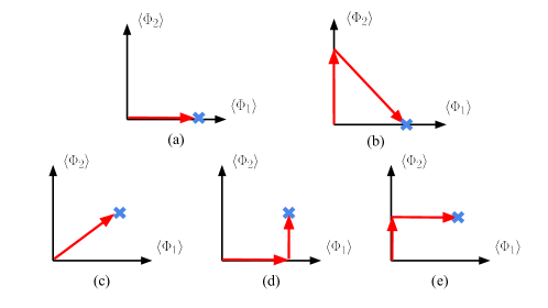
Figure 1: The path of phase transitions in the model with two classical fields $\left\langle\Phi_{1}\right\rangle$ and $\left\langle\Phi_{2}\right\rangle$. The blue cross marks represent the global minimum point of the potential at zero temperature. The value of $\left\langle\Phi_{2}\right\rangle$ is zero in (a) and (b) phase transitions, while it is nonzero in (c–e) phase transitions, respectively.

In the phase transitions of Fig. 1-(a) and -(b), the classical field of the additional scalar field $\left\langle\Phi_{2}\right\rangle$ at the blue cross marks is zero after the phase transition, while this value in Fig. 1-(c)–(e) is nonzero. We will focus on the two-step phase transition pattern shown in Fig. 1-(b), in which a broken global symmetry is restored after electroweak symmetry breaking (EWSB).

We will focus on the two-step phase transition shown in Fig. 1-(b). According to this phase transition path, a global symmetry in the potential is broken during the phase transition. After the phase transition, the broken symmetry can be restored in the current universe. Such a multi-step phase transition is significant to explain the phenomena beyond the standard model; dark matter existence FileviezPerez:2008bj ; Cui:2011qe ; Cline:2012hg ; Patel:2012pi ; Fairbairn:2013uta ; Alanne:2014bra ; Blinov:2015sna ; Baker:2016xzo ; Grzadkowski:2018nbc ; Baker:2018vos ; Bian:2018bxr ; Ghorbani:2019itr ; Robens:2019kga ; Chen:2019ebq ; Chiang:2019oms ; Bell:2020gug ; Chiang:2020yym , baryon asymmetry of the universe Profumo:2007wc ; Espinosa:2011ax ; Espinosa:2011eu ; Profumo:2014opa ; Inoue:2015pza ; Tenkanen:2016idg ; Vaskonen:2016yiu ; Kurup:2017dzf ; Chen:2017qcz ; Ramsey-Musolf:2017tgh ; Chala:2018opy ; Gould:2019qek ; Caprini:2019egz ; Kozaczuk:2019pet ; Ramsey-Musolf:2019lsf ; Senaha:2020mop . Furthermore, the phase transition in the second path of Fig. 1-(b) can be strong because the barrier shows up in the potential at the zero temperature by tree-level effects, like Ref. Espinosa:2011ax . We will show the conditions in which the two-step phase transition happens in this general model. For the EWPT in Fig. 1-(b), the first (second) step relies on the thermal loop (tree-level) effects, and thus the sizable barrier could be generated in the second step by the tree-level effects. The detectable GW spectrum is mainly produced by the second step since the tree-level effect is the dominant contribution to this phase transition path. On the other hand, the first-order EWPT in Fig. 1-(a) can be realized by finite thermal effects only. Since the sources of the barrier are different between the one-step and the two-step phase transitions, the temperature for starting the EWPT of the Fig. 1-(a) is higher than that of the Fig. 1-(b). Therefore, we may distinguish the patterns of the EWPT in Fig. 1-(a) and -(b) by the GW observation.

In the following, we introduce the model’s detail with additional isospin $N$-plet scalar field $\Phi_{2}$ with discrete $Z_{2}$ symmetry in Sec. 2 and 3. Furthermore, we use the high-temperature approximation to discuss the condition of the multi-step phase transition analytically in Sec. 4. In Sec. 6, we numerically discuss the dynamics of the EWPT being able to restore the $Z_{2}$ symmetry after the EWPT and show detectability of the GW spectrum produced from the first-order EWPT of Fig. 1-(a) and -(b). The conclusion is drawn in Sec. 7.

2 General Form of $\mathbb{Z}_{2}$ $N$-plet Scalar Model

We first present a general form of the potential under the extended model with an isospin $N$-plet scalar $\Phi_{2}\sim(I_{2},Y_{2})$ under $SU(2)_{L}\times U(1)_{Y}$ gauge symmetry. To make a complete analysis, in this section, we use $2I_{2}=N-1$ fundamental indices instead to present the isospin $N$-plet field $\Phi_{2}$, which is given by

$$(\Phi_{2})_{i_{1}\cdots i_{2I_{2}}}=C^{\mathcal{I}}_{i_{1}\cdots i_{2I_{2}}}\Phi_{2}^{\mathcal{I}},\quad\Phi_{2}^{\mathcal{I}}=\frac{1}{\sqrt{2}}\left(\begin{array}[]{crcccccc}s_{I_{2}}+i\sigma_{I_{2}}\\ s_{I_{2}-1}+i\sigma_{I_{2}-1}\\ \vdots\\ s_{-I_{2}}+i\sigma_{-I_{2}}\end{array}\right).$$ (5)

The cursive letter represents the weight of each component, whose real and imaginary parts are regarded as $s_{\mathcal{I}}$ and $\sigma_{\mathcal{I}}$, respectively. The scalar potential using the form $\Phi_{2}^{\mathcal{I}}$ was discussed in Ref. Ramsey-Musolf:2021ldh , however, we do not adapt this form in the following discussion. If $\Phi_{2}$ is real, then $s_{-\mathcal{I}}=(-1)^{\mathcal{I}}s_{\mathcal{I}}$, $\sigma_{-\mathcal{I}}=(-1)^{\mathcal{I}+1}\sigma_{\mathcal{I}}$ and $\Phi_{2}^{0}=s_{0}$. The generalized Clebsh-Gordan coefficients $C^{\mathcal{I}}_{i_{1}\cdots i_{2I_{2}}}$, which is symmetric under all permutations of $i_{n}$, can be calculated through construction of a $j=I_{2}$ representation of $SU(2)_{L}$ as

$$C^{\mathcal{I}}_{i_{1}\cdots i_{2I_{2}}}=\sqrt{\frac{(I_{2}+\mathcal{I})!(I_{2}-\mathcal{I})!}{(2I_{2})!}}\delta^{\mathcal{I}}_{\sum_{n}(3/2-i_{n})},\quad i_{n}=1\text{ or }2.$$ (6)

The Clebsh-Gordan coefficients satisfy the normalization condition

$$C^{\mathcal{I}}_{i_{1}\cdots i_{2I_{2}}}C^{\mathcal{J}}_{j_{1}\cdots j_{2I_{2}}}\prod_{n=1}^{2I_{2}}\epsilon^{i_{n}j_{n}}=\delta^{\mathcal{IJ}},$$ (7)

where $\epsilon^{ij}=i\sigma^{2}$ is the 2-dimensional anti-symmetric tensor. The complex conjugate field transforming under the same representation of $SU(2)_{L}$ can be written as

$$(\Phi_{2})^{*}_{i_{1}\cdots i_{2I_{2}}}=(\Phi_{2})^{*j_{1}\cdots j_{2I_{2}}}\prod_{n=1}^{2I_{2}}\epsilon_{i_{n}j_{n}}\equiv[(\Phi_{2})_{j_{1}\cdots j_{2I_{2}}}]^{*}\prod_{n=1}^{2I_{2}}\epsilon_{i_{n}j_{n}}.$$ (8)

The SM-like Higgs is

$$(\Phi_{1})_{i}=\left(\begin{array}[]{crcccccc}G^{+}\\ \frac{1}{\sqrt{2}}\left(h+iG^{0}\right)\end{array}\right),\quad(\Phi_{1})^{*}_{i}=\epsilon_{ij}(\Phi_{1})^{*j}=\left(\begin{array}[]{crcccccc}\frac{1}{\sqrt{2}}\left(h-iG^{0}\right)\\ -G^{-}\end{array}\right).$$ (13)

Under this notation, the Lagrangian of the scalar sector is

$${\cal L}_{\text{Scalar}}=(D_{\mu}\Phi_{1})^{\dagger}(D^{\mu}\Phi_{1})+(D^{\mu}\Phi_{2})^{*}_{i_{1}\cdots i_{2I_{2}}}(D_{\mu}\Phi_{2})_{j_{1}\cdots j_{2I_{2}}}\prod_{n=1}^{2I_{2}}\epsilon^{i_{n}j_{n}}-V_{0}(\Phi_{1},\Phi_{2}),$$ (14)

where $D_{\mu}=\partial_{\mu}-igT^{a}W_{\mu}^{a}-ig^{\prime}YB_{\mu}$. Here $g$ and $g^{\prime}$ are ${\text{SU}}(2)_{L}$ and $U(1)_{Y}$ gauge couplings respectively, and $T^{a}$ is the generator of ${\text{SU}}(2)_{L}$ for corresponding representation. Also note that in principle, the factor in the production should be fully symmetrized for $i_{n}$ and $j_{n}$, but here we leave it implicit since these indices are symmetric in the fields. These scalar fields transform as $\Phi_{1}\to\Phi_{1}$ and $\Phi_{2}\to-\Phi_{2}$ under the assumed $\mathbb{Z}_{2}$ symmetry. For simplicity, other fields in the model are all $\mathbb{Z}_{2}$ even.

The general form of the potential can be obtained by the Young tableau method. The mass terms or the quadratic terms read as

$$\Delta V_{0}=-\mu_{1}^{2}(\Phi_{1})^{*i}(\Phi_{1})_{i}-\mu_{2}^{2}(\Phi_{2})^{*}_{i_{1}\cdots i_{2I_{2}}}(\Phi_{2})_{j_{1}\cdots j_{2I_{2}}}\prod_{n=1}^{2I_{2}}\epsilon^{i_{n}j_{n}}.$$ (15)

with the symmetrization over every group of indices implicit. The interaction terms are given as

$$\Delta V_{0} =(\Phi_{1})^{*}_{i}(\Phi_{1})_{j}(\Phi_{2})^{*}_{k_{1}\cdots k_{2I_{2}}}(\Phi_{2})_{l_{1}\cdots l_{2I_{2}}}\times\left[a_{0}K_{0}^{ijk_{1}\cdots l_{2I_{2}}}+a_{1}K_{1}^{ijk_{1}\cdots l_{2I_{2}}}\right]$$

$$\phantom{=}+(\Phi_{1})_{i}(\Phi_{1})_{j}(\Phi_{1})^{*}_{k}(\Phi_{1})^{*}_{l}\times\lambda_{1}\epsilon^{ik}\epsilon^{jl}$$

$$\phantom{=}+(\Phi_{2})_{i_{1}\cdots i_{2I_{2}}}(\Phi_{2})_{j_{1}\cdots j_{2I_{2}}}(\Phi_{2})^{*}_{k_{1}\cdots k_{2I_{2}}}(\Phi_{2})^{*}_{l_{1}\cdots l_{2I_{2}}}\times\sum_{m=0}^{\lfloor I_{2}\rfloor}b_{m}C_{m}^{i_{1}\cdots l_{2I_{2}}},$$ (16)

where the factors are

$$K_{0}^{ijk_{1}\cdots l_{2I_{2}}} =\frac{1}{[(2I_{2})!]^{2}}\left[\epsilon^{ij}\prod_{n=1}^{2I_{2}}\epsilon^{k_{n}l_{n}}+(\text{all perms of }k,l)\right],$$ (17)

$$K_{1}^{ijk_{1}\cdots l_{2I_{2}}} =\frac{1}{[(2I_{2})!]^{2}}\left[\epsilon^{ik_{1}}\epsilon^{jl_{1}}\prod_{n=1}^{2I_{2}-1}\epsilon^{k_{n}l_{n}}+(\text{all perms of }k,l)\right],$$ (18)

$$C_{m}^{i_{1}\cdots l_{2I_{2}}} =\frac{1}{[(2I_{2})!]^{4}}\left[\prod_{n=1}^{2m}\epsilon^{i_{n}j_{n}}\epsilon^{k_{n}l_{n}}\prod_{n=2m+1}^{2I_{2}}\epsilon^{i_{n}k_{n}}\epsilon^{j_{n}l_{n}}+(\text{all perms of }i,j,k,l)\right],$$ (19)

and $\lfloor n\rfloor$ means the rounding down of $n$. The explicit symmetrization of indices is important to calculate Feynman diagrams correctly. Also, note that the terms proportional to $a_{1}$ do not exist when $I_{2}=0$.

When the isospin and hypercharge of $\Phi_{2}$ take some special values, there will be additional gauge-invariant terms. For complex $\Phi_{2}$ with even $2I_{2}$ and $Y_{2}=0$, one can add these terms:

$$\Delta V_{0} =(\Phi_{1})^{*}_{i}(\Phi_{1})_{j}(\Phi_{2})_{k_{1}\cdots k_{2I_{2}}}(\Phi_{2})_{l_{1}\cdots l_{2I_{2}}}\times a_{0}^{\prime}K_{0}^{ijk_{1}\cdots l_{2I_{2}}}$$

$$\phantom{=}+(\Phi_{2})_{i_{1}\cdots i_{2I_{2}}}(\Phi_{2})_{j_{1}\cdots j_{2I_{2}}}(\Phi_{2})_{k_{1}\cdots k_{2I_{2}}}(\Phi_{2})_{l_{1}\cdots l_{2I_{2}}}\times\sum_{m=0}^{\lfloor I_{2}/2\rfloor}b_{m}^{\prime}C_{m}^{i_{1}\cdots l_{2I_{2}}}$$

$$\phantom{=}+(\Phi_{2})_{i_{1}\cdots i_{2I_{2}}}(\Phi_{2})_{j_{1}\cdots j_{2I_{2}}}(\Phi_{2})_{k_{1}\cdots k_{2I_{2}}}(\Phi_{2})^{*}_{l_{1}\cdots l_{2I_{2}}}\times\sum_{m=0}^{\lfloor I_{2}/2\rfloor}b_{m}^{\prime\prime}C_{m}^{i_{1}\cdots l_{2I_{2}}}+\mathrm{h.c.}.$$ (20)

However, as the complex $\Phi_{2}$ is in a real representation under this case, it can be divided into two real components with different CP properties. For odd $2I_{2}$ with $Y_{2}=0$ and $\pm 1/2$,

$$\Delta V_{0}^{(Y_{2}=0)} =(\Phi_{1})^{*}_{i}(\Phi_{1})_{j}(\Phi_{2})_{k_{1}\cdots k_{2I_{2}}}(\Phi_{2})_{l_{1}\cdots l_{2I_{2}}}\times a_{1}^{\prime}K_{1}^{ijk_{1}\cdots l_{2I_{2}}}+\mathrm{h.c.},$$ (21)

$$\Delta V_{0}^{(Y_{2}=1/2)} =(\Phi_{1})_{i}(\Phi_{1})_{j}(\Phi_{2})^{*}_{k_{1}\cdots k_{2I_{2}}}(\Phi_{2})^{*}_{l_{1}\cdots l_{2I_{2}}}\times a_{1}^{\prime}K_{1}^{ijk_{1}\cdots l_{2I_{2}}}+\mathrm{h.c.}.$$ (22)

The discussion above on the general potential is valid under the case that the new scalar $\Phi_{2}$ is complex. The potential for a real one will be a bit simpler due to the flavor symmetry. Only the $a_{0}$- and $b_{m}$- with $m$ up to $\lfloor I_{2}/2\rfloor$ terms in Eq. (2) are non-redundant. Also, there should be a $1/2$ factor before $\mu_{2}^{2}$ in Eq. (15).

3 The One-loop Effective Potential

To analyze the behavior of the effective potential as the temperature varieties, one needs to evaluate the effective potential at least up to the one-loop level. In our work, it is assumed that only the charge-neutral components of scalars generate VEVs, so we only consider the effective potential of these components. $h$ and $s_{-Y_{2}}$ are the CP-even neutral components of $\Phi_{1}$ and $\Phi_{2}$ respectively, and we here define classical scalar fields as $h_{1}$ and $h_{2}$ for $h$ and $s_{-Y_{2}}$ fields, respectively. The effective potential with the finite temperature effects is given as

$$V_{eff}\left(h_{1},h_{2},T\right)=V_{0}(h_{1},h_{2})+V_{\text{CW}}(h_{1},h_{2})+\Delta V_{T}(h_{1},h_{2},T)+V_{T}^{\rm ring}(h_{1},h_{2},T),$$ (23)

where we have included the daisy resummation contributions to avoid IR divergence.

Generally, each term in Eq. (23) are all dependent on the field-dependent mass as

$$V_{\text{CW}} =\sum_{i}\frac{n_{i}}{64\pi^{2}}\,M^{4}_{i}\left(h_{1},h_{2}\right)\,\left[\ln\left(\frac{M^{2}_{i}\left(h_{1},h_{2}\right)}{Q^{2}}\right)-c_{i}\right],$$ (24)

$$\Delta V_{T} =\frac{T^{4}}{2\pi^{2}}\Bigl{\{}\sum_{i={\rm bosons}}n_{i}\int_{0}^{\infty}dxx^{2}\ln\left[1-\exp\left(-\sqrt{x^{2}+(M_{i}\left(h_{1},h_{2}\right)/T)^{2}}\right)\right]$$

$$+\sum_{i={\rm fermions}}n_{i}\int_{0}^{\infty}dxx^{2}\ln\left[1+\exp\left(-\sqrt{x^{2}+(M_{i}\left(h_{1},h_{2}\right)/T)^{2}}\right)\right]\Bigl{\}},$$ (25)

$$V_{T}^{\rm ring} =\frac{T}{12\pi}\sum_{\rm i=bosons}n_{i}\left((M_{i}^{2}(h_{1},h_{2}))^{3/2}-(M_{i,T}^{2}(h_{1},h_{2}))^{3/2}\right).$$ (26)

Here the Coleman-Weinberg potential Eq. (24) is calculated under $\overline{\text{MS}}$ scheme with $Q$ the renormalization scale, and $c_{i}=3/2$ for scalars and fermions and $5/6$ for gauge bosons. The index $i$ in the summation runs over all the fields in the model, with the field-dependent masses given by square roots of the eigenvalues of the mass-squared matrix

$$M_{ij}^{2}(h_{1},h_{2})=\frac{\partial^{2}V_{0}}{\partial\phi_{i}\partial\phi_{j}}\Bigg{|}_{h_{1},h_{2}}$$ (27)

for bosons and similar for fermions. A general expression for the field-dependent masses of scalars is hard to obtain, and in Appendix A, we present the results of the singlet, doublet, and triplet extended models. For gauge bosons and fermions, they are given as

$$M_{W}^{2}=\frac{1}{4}g^{2}\left(h_{1}^{2}+I_{W}^{2}h_{2}^{2}\right),~{}M_{Z}^{2}=\frac{1}{4}(g^{2}+g^{\prime 2})\left(h_{1}^{2}+4Y_{2}^{2}h_{2}^{2}\right),~{}M_{t}^{2}=\frac{1}{2}y_{t}^{2}h_{1}^{2},$$ (28)

with $I_{W}^{2}=2I_{2}(I_{2}+1)-2Y_{2}^{2}$.

The $M_{i,T}^{2}(h_{1},h_{2})$ in Eq. (26) are the eigenvalues of thermal-corrected field-dependent mass-squared matrix, which is given by adding the Debye mass term $\Pi_{ij}(T)$ to the mass-squared matrix. The Debye mass term can be regarded as an effective mass term induced by the plasma, whose leading order comes from the one-loop diagram. For example, the following shows the contribution from the $b_{m}$-terms to the Debye mass of $\Phi_{2}$:

$$(\Delta\Pi^{\Phi_{2}\Phi_{2}^{*}})^{i_{1}\cdots j_{2I_{2}}} =\begin{gathered}\leavevmode\hbox to40.23pt{\vbox to40.23pt{\text{[drawing]}}}\end{gathered}$$ (30)

$$=-2i\sum_{m=0}^{\lfloor I_{2}\rfloor}b_{m}\times\left\{\left[\prod_{n=1}^{2m}\epsilon^{i_{n}k_{n}}\epsilon^{j_{n}l_{n}}\prod_{n=2m+1}^{2I_{2}}\epsilon^{i_{n}j_{n}}\epsilon^{k_{n}l_{n}}+(j\leftrightarrow l)\right]\right.$$

$$\phantom{=}+{\text{all perms of }i,j,k,l}\Bigg{\}}\left[\frac{1}{(2I_{2})!}\right]^{4}\times\prod_{n=1}^{2I_{2}}\epsilon_{k_{n}l_{n}}\,\sum\!\!\!\!\!\!\!\int_{K}\frac{1}{k^{2}+\omega_{n}^{2}}.$$ (31)

The ‘sumint’ symbol stands for the integral over 3D space and the summation over all the Matsubara mode $\omega_{n}$ with a $T$ prefactor. The full result of Debye mass for scalars are

$$\Pi^{\Phi_{1}\Phi_{1}^{*}}_{ij} =\delta_{ij}T^{2}\left[\frac{\lambda_{1}}{2}+\frac{3g^{2}}{16}+\frac{g^{\prime 2}}{16}+\frac{y_{t}^{2}}{4}+\frac{1}{6}(2I_{2}+1)\left(a_{0}+\frac{1}{2}a_{1}\right)\right],$$ (32)

$$\Pi^{\Phi_{2}\Phi_{2}}_{\mathcal{IJ}} =\delta_{\mathcal{IJ}}T^{2}\left[\frac{g^{2}}{4}\left(I_{2}^{2}+I_{2}\right)+\frac{g^{\prime 2}}{4}Y_{2}^{2}+\frac{1}{3}\sum_{m=0}^{\lfloor I_{2}/2\rfloor}f(I_{2},m)b_{m}+\frac{1}{6}a_{0}\right]$$ (33)

for real $\Phi_{2}$ and

$$\Pi^{\Phi_{2}\Phi_{2}^{*}}_{\mathcal{IJ}} =\delta_{\mathcal{I},\mathcal{J}}T^{2}\left[\frac{g^{2}}{4}\left(I_{2}^{2}+I_{2}\right)+\frac{g^{\prime 2}}{4}Y_{2}^{2}+\frac{1}{6}\sum_{m=0}^{\lfloor I_{2}\rfloor}b_{m}\left(\frac{2I_{2}+1}{2m+1}+1\right)+\frac{1}{6}a_{0}+\frac{1}{12}a_{1}\right]$$ (34)

for complex $\Phi_{2}$, while for even $2I_{2}$ and $Y_{2}=0$ extra terms contribute as

$$\Delta\Pi^{\Phi_{2}\Phi_{2}^{*}}_{\mathcal{IJ}} =\delta_{\mathcal{I},-\mathcal{J}}(-1)^{j-\mathcal{I}}\frac{T^{2}}{3}\sum_{m=0}^{\lfloor I_{2}/2\rfloor}f(I_{2},m)\left(\begin{array}[]{cc}\operatorname{Re}(b_{m}^{\prime\prime})&-\operatorname{Im}(b_{m}^{\prime\prime})\\ -\operatorname{Im}(b_{m}^{\prime\prime})&-\operatorname{Re}(b_{m}^{\prime\prime})\end{array}\right).$$ (37)

The non-diagonal term in Eq. (37) indicates the mixing between $s_{\mathcal{I}}$ and $a_{\mathcal{I}}$ and

$$f(I_{2},m) =\frac{2I_{2}+1}{2m+1}+\frac{2I_{2}+1}{2I_{2}-2m+1}+1.$$ (38)

For gauge bosons, only the longitudinal modes receive contributions from thermal loops at leading order, which leads to

$$\Pi^{WW}_{IJ} =\delta_{IJ}g^{2}T^{2}\left[\frac{11}{6}+\frac{1}{9}I_{2}\left(1+I_{2}\right)\left(1+2I_{2}\right)\right],$$ (39)

$$\Pi^{BB} =g^{\prime 2}T^{2}\left[\frac{11}{6}+\frac{1}{3}\left(1+2I_{2}\right)Y_{2}^{2}\right].$$ (40)

If $\Phi_{2}$ is real, the terms related to $I_{2}$ should be reduced by half.

4 Analysis of Two-step Phase Transition

Since we are focusing on a two-step phase transition, we would like to give an analytic calculation on the possibility of a two-step phase transition. To simplify the calculation, we will take the leading terms in Eq. (23) only when we derive the analytic conditions. The leading terms are reparametrized as

$$V_{\text{eff}}\left(h_{1},h_{2},T\right) =\frac{1}{2}\left(-\hat{\mu}_{1}^{2}+D_{1}T^{2}\right)h_{1}^{2}+\frac{1}{2}\left(-\hat{\mu}_{2}^{2}+D_{2}T^{2}\right)h_{2}^{2}+\frac{1}{4}\hat{\lambda}_{12}h_{1}^{2}h_{2}^{2}+\frac{1}{4}\hat{\lambda}_{1}h_{1}^{4}+\frac{1}{4}\hat{\lambda}_{2}h_{2}^{4},$$ (41)

with the relation between original and hatted parameters given by

$$\hat{\mu_{1}}^{2}=\mu_{1}^{2},~{}\hat{\mu_{2}}^{2}=(-1)^{I_{2}}\mu_{2}^{2},~{}\hat{\lambda}_{12}=(-1)^{I_{2}}2a_{0},~{}\hat{\lambda}_{1}=\lambda_{1},~{}\hat{\lambda}_{2}=4\sum_{m=0}^{\lfloor I_{2}/2\rfloor}b_{m}F(I_{2},0,m).$$ (42)

for real $\Phi_{2}$ and

$$\hat{\mu_{1}}^{2}=\mu_{1}^{2},~{}\hat{\mu_{2}}^{2}=\mu_{2}^{2},~{}\hat{\lambda}_{12}=a_{0}+\frac{I_{2}-Y_{2}}{2I_{2}}a_{1},~{}\hat{\lambda}_{1}=\lambda_{1},~{}\hat{\lambda}_{2}=\sum_{m=0}^{\lfloor I_{2}\rfloor}b_{m}F(I_{2},Y_{2},m).$$ (43)

for complex $\Phi_{2}$. The contributions from extra terms are

$$\Delta\hat{\lambda}_{12}=(-1)^{I_{2}}2\operatorname{Re}(a_{0}^{\prime}),~{}\Delta\hat{\lambda}_{2}=\sum_{m=0}^{\lfloor I_{2}/2\rfloor}2F(I_{2},0,m)\operatorname{Re}(b_{m}^{\prime}+(-1)^{I_{2}}b_{m}^{\prime\prime}),$$ (44)

when $2I_{2}$ is even and $Y_{2}=0$, and

$$\Delta\hat{\lambda}_{12}=(-1)^{I_{2}-1/2}\frac{I_{2}+1/2}{I_{2}}\operatorname{Re}(a_{1}^{\prime}).$$ (45)

when $2I_{2}$ is odd and $Y_{2}=1/2$. The definition of the function $F$ is

$$F(I,Y,m)= \sum_{s=0}^{2m}\left[\frac{(I-Y)!(I+Y)!}{(2I)!}\right]^{2}\left[\frac{(2m)!}{s!(2m-s)!}\right]^{2}$$

$$\times\frac{[(2I-2m)!]^{2}}{(I-Y-s)!(I+Y-s)!(I-Y-2m+s)!(I+Y-2m+s)!}$$ (46)

with all terms in factorials non-negative. $D$-terms can be extracted directly from the Debye mass terms

$$D_{1}=\Pi_{22}^{\Phi_{1}\Phi_{1}^{*}}/T^{2},\quad D_{2}=\Pi_{Y_{2}Y_{2}}^{\Phi_{2}\Phi_{2}^{(*)}}/T^{2}.$$ (47)

The five parameters in the potential $\hat{\mu}_{1}^{2}$, $\hat{\mu}_{2}^{2}$, $\hat{\lambda}_{1}$, $\hat{\lambda}_{2}$ and $\hat{\lambda}_{12}$ will be replaced by five input parameters $v$, $m_{h}$, $m_{H}$, $\hat{\lambda}_{2}$ and $\hat{\lambda}_{12}$ in this section, where $v=246$ GeV, $m_{h}=125$ GeV and $m_{H}$ is the mass of the additional CP-even neutral scalar. At the tree level, their relation is

$$\hat{\mu}_{1}^{2}=\frac{1}{2}m_{h}^{2},~{}\hat{\mu}_{2}^{2}=\frac{1}{2}\lambda_{12}v^{2}-m_{H}^{2},~{}\hat{\lambda}_{1}=\frac{m_{h}^{2}}{2v^{2}}.$$ (48)

In the following, we will discuss the conditions and the strength of the two-step phase transition with the hat marks implicit.

4.1 Conditions for Two-step Transition

Two local minimums must appear successively during the two-step phase transition when cooling down. In addition, the SM vacuum $v=246{\text{GeV}}$ should be the global minimum. Here we enumerate three necessary conditions for a two-step phase transition as follows:

Two different local minima

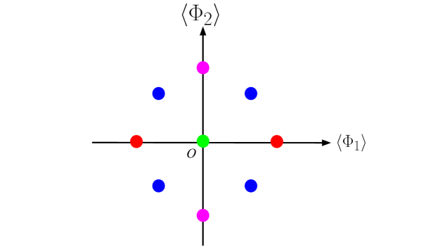
Figure 2: Extremums in the tree-level potential.

The tree-level potential has nine stationary points, among which there are four different points as shown in Fig. 2 marked by green, red, blue, and magenta if a $\mathbb{Z}_{2}\times\mathbb{Z}_{2}$ symmetry is considered. The green point lies at the origin, and the red and magenta points are along $h_{1}$ and $h_{2}$ axes, respectively. From the Hesse matrix

$${\cal H}=\begin{pmatrix}-\mu_{1}^{2}+3\lambda_{1}h_{1}^{2}+\lambda_{12}h_{2}^{2}/2&\lambda_{12}h_{1}h_{2}\\ \lambda_{12}h_{1}h_{2}&-\mu_{2}^{2}+3\lambda_{2}h_{2}^{2}+\lambda_{12}h_{1}^{2}/2\end{pmatrix},$$ (49)

one can find that the only possibility for two local minima happens when the blue and green points are saddle points. The definiteness of the Hesse matrix requires

$$\lambda_{12}\mu_{1}^{2}>2\lambda_{1}\mu_{2}^{2}>0,\quad\lambda_{12}\mu_{2}^{2}>2\lambda_{2}\mu_{1}^{2}>0.$$ (50)

Combining these two inequalities one can put a constraint on $\lambda_{12}$ as

$$\lambda_{12}>2\sqrt{\lambda_{1}\lambda_{2}}.$$ (51)

The global minimum

As is discussed at the beginning of this subsection, the global minimum should lie at the SM-Higgs axis, with $h_{1}=246{\text{GeV}}$, which requires

$$\frac{\mu_{1}^{4}}{\lambda_{1}}>\frac{\mu_{2}^{4}}{\lambda_{2}}.$$ (52)

$h_{2}$ vacuum appears first when cooling down

As is indicated in Fig. 1-(b), a two-step phase transition requires that a local minimum along the $h_{2}$ axis appears first when cooling down. Along each axis ($h_{2}=0$ or $h_{1}=0$), it could be found that whether there is another extremum besides the origin depends on the quadratic term, $-\mu_{i}^{2}+D_{i}T^{2}$. At high temperatures, all coefficients in the potential are positive, and the global minimum lies at the origin. When the temperature drops and the quadratic term becomes negative, the local minimum changes to $h_{i}^{2}\sim(-\mu_{i}^{2}+D_{i}T^{2})/\lambda_{i}$ along each axis. We could define the turning temperature $T_{i}$ at which the quadratic coefficient changes sign, given by $T_{i}^{2}=\mu_{i}^{2}/D_{i}$. Therefore, approximately the criterion for a two-step phase transition can be presented as

$$T_{2}>T_{1},~{}\text{i.e. }\frac{\mu_{2}^{2}}{D_{2}}>\frac{\mu_{1}^{2}}{D_{1}},$$ (53)

where $D_{1,2}$ are defined in Eq. (47).

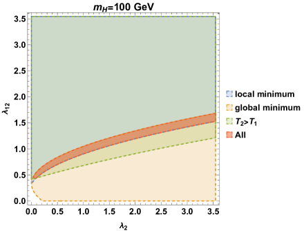
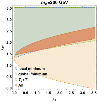
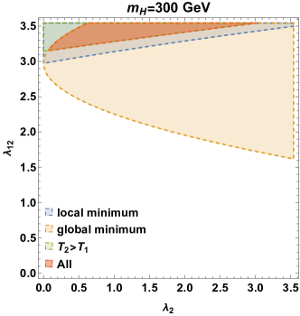
Figure 3: Parameter regions that satisfies the conditions of Eqs. (50), (52) and (53), with $(I_{2},Y_{2})=(1/2,1/2)$ and $m_{H}=100,200,300\,{\text{GeV}}$. The region enclosed by blue, yellow, and green dashed lines corresponds to each condition, and the red is the union region. It could be found that the allowed regions for $\lambda_{12}$ are narrow belts scaling as $m_{H}$, and the upper bounds are set by the ‘global minimum’ condition. Also, the lower bounds from ‘local minimum’ and $T_{2}>T_{1}$ are quite close, indicating that the phase transition goes through two steps given the condition that there are two local minima.

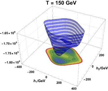
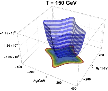
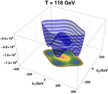
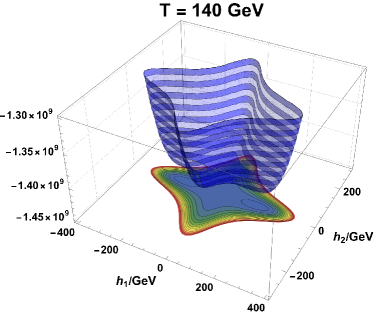
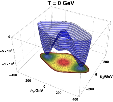
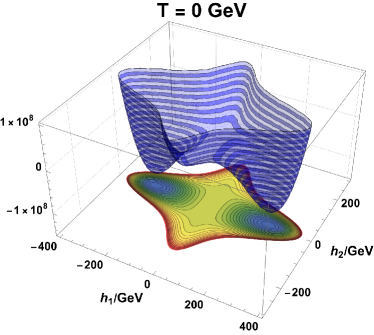
(a)

Figure 4: The potential as the temperature varieties. The left column shows the effective potential at $T=150~{}{\text{GeV}}$, $118~{}{\text{GeV}}$ and $T=0~{}{\text{GeV}}$ respectively with $\lambda_{2}=\lambda_{12}=2.0,~{}m_{H}=200~{}{\text{GeV}}$ and $(I_{2},Y_{2})=(1/2,1/2)$, while the right is $T=150~{}{\text{GeV}}$, $140{\text{GeV}}$ and $T=0~{}{\text{GeV}}$ respectively with $\lambda_{2}=0.25,~{}\lambda_{12}=3.02,~{}m_{H}=300~{}{\text{GeV}}$ and $(I_{2},Y_{2})=(1,1)$. Only the left case goes through a two-step phase transition.

We plot the parameter region that satisfies the three conditions above in Fig. 3. The region enclosed by blue, yellow, and green dashed lines corresponds to each condition, as shown in the legends, and the red one is the overlap region. It could be found that $\lambda_{12}$ is allowed in a narrow band in each plot, scaling as $m_{H}^{2}$. The upper bounds for $\lambda_{12}$ are set by the ‘global minimum’ condition. In contrast, the lower bounds from the ‘local minimum’ and $T_{2}>T_{1}$ conditions are quite close, indicating that the phase transition goes through two steps given the condition that there are two local minima. We find that the two-step phase transition happens in a narrow region of the $\lambda_{12}$ couplings. This coupling should be moderately large and must be larger as the mass of the $\Phi_{2}$ increases. Furthermore, we find that as the isospin increases, the required $\lambda_{12}$ coupling should be larger to realize a two-step phase transition.

Fig. 4 shows how the potential evolves when the temperature drops. The numerical analysis of the effective potential includes the effect of tree-level, one-loop, and Daisy-resummed parts. The left column presents the case that $\lambda_{2}=\lambda_{12}=2.0,~{}m_{H}=200~{}{\text{GeV}}$ and $(I_{2},Y_{2})=(1/2,1/2)$. This set of parameters satisfies three conditions and does realize a two-step phase transition. By contrast, the right one only goes through one step, with the parameter $\lambda_{2}=0.25,~{}\lambda_{12}=3.02,~{}m_{H}=300~{}{\text{GeV}}$ and $(I_{2},Y_{2})=(1,1)$ lying outside the allowed region, even when there are two local minima at zero temperature.

4.2 Potential Barriers for Two-step Transition

In the following, we will discuss the possibility of two strong first-order phase transitions (SFOPTs) in Fig. 1-(b) by the criterion that $v(T_{C})/T_{C}\gtrsim 1$, where $T_{C}$ denotes the critical temperature at which the potential values at two local minima degenerate. To evaluate the criterion in the first step (green $\to$ magenta), we could analyze the potential along the $h_{2}$ axis. However, Eq. (41) cannot generate a barrier separating the origin and another local minimum because there only exists a quadratic and a quartic term. It is necessary to add the effects of the next-to-leading order, which is roughly

$$V_{\text{eff}}\left(0,h_{2},T\right)\sim\frac{1}{2}(-\mu_{2}^{2}+D_{2}T^{2})h_{2}^{2}-E_{2}Th_{2}^{3}+\frac{1}{4}\lambda_{2}h_{2}^{4}.$$ (54)

The cubic term $E_{2}$ comes from the thermal loops of bosons, and the contributions from gauge bosons and scalars are

$$E_{2}^{g} =\frac{1}{16\pi}g^{3}I_{W}^{3}+\frac{1}{4\pi}(g^{2}+g^{\prime 2})^{3/2}Y_{2}^{3},$$

$$E_{2}^{\Phi} \sim\frac{2I_{2}+1}{6\pi}\sum_{m}b_{m}\times{\cal O}(1)\sim\frac{2I_{2}+1}{6\pi}\lambda_{2}.$$ (55)

Here the explicit expression of $E_{2}^{\Phi}$ requires a specific model, and we only give a rough result with the approximation that $\lambda_{2}\sim\sum_{m}b_{m}F(I_{2},Y_{2},m)\sim\sum_{m}b_{m}$. The criterion for an SFOPT shows that

$$\frac{v_{2}(T_{C,1})}{T_{C,1}}=\frac{2E_{2}}{\lambda_{2}}\gtrsim 1\quad\Rightarrow\quad\left(1-\frac{2I_{2}+1}{3\pi}\right)\lambda_{2}\lesssim 2E_{2}^{g},$$ (56)

where $v_{2}$ is the value of the local minimum and $T_{C,1}$ stands for the critical temperature at which $V_{\text{eff}}(0,0,T_{C,1})=V_{\text{eff}}(0,v_{2}(T_{C,1}),T_{C,1})$. This estimation sets an upper bound for $\lambda_{2}$ under low representations $N\leq 9$, and for $N\leq 4$, which indicates that an SFOPT in the first step may require a high representation of $SU(2)_{L}$. In Sec. 6 we will give a numerical analysis of the doublet model.

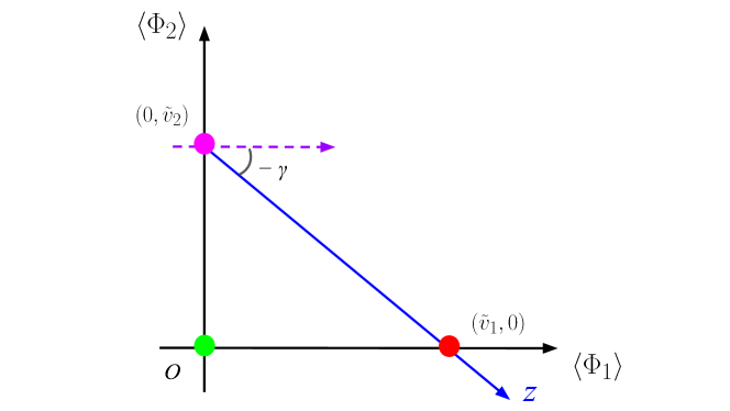
Figure 5: Polar coordinates in the effective potential. $z$ and $\gamma$ are a radius and an angle in the coordinates.

For the second step of the EWPT (i.e., the path of magenta $\to$ red) in Fig. 1-(b), we choose to reparametrize the field $h_{1}$ and $h_{2}$ by a polar coordinate $(z,\gamma)$ as is shown in Fig. 5. The center of the polar coordinate is set to be the local minimum along $h_{2}$ axis. The relation between two coordinates are given by $h_{1}=z\cos\gamma$ and $h_{2}=v_{2}(T)+z\sin\gamma$, and the coordinates of two minima are called $(0,0)$ and $(\tilde{z},\tilde{\gamma})$. Since a barrier already exists between two minima due to condition Eq. (50), it is sufficient to use the leading-order potential Eq. (23) to describe the phase transition and therefore

$$v_{1}(T)^{2}=\frac{\mu_{1}^{2}-D_{1}T^{2}}{\lambda_{1}},~{}v_{2}(T)^{2}=\frac{\mu_{2}^{2}-D_{2}T^{2}}{\lambda_{2}},$$

$$\tilde{z}(T)^{2}=v_{1}(T)^{2}+~{}v_{2}(T)^{2},~{}\tan\tilde{\gamma}(T)=-\frac{v_{2}(T)}{v_{1}(T)}.$$ (57)

Under the polar coordinates, the effective potential Eq. (23) is given by

$$V_{\text{eff}}\left(z,\gamma,T\right) =C_{0}+C_{2}z^{2}+C_{3}z^{3}+C_{4}z^{4},$$ (58)

where

$$C_{0} =-\frac{1}{4}\lambda_{2}v_{2}(T)^{4},\quad C_{2}=\lambda_{2}v_{2}(T)^{2}s_{\gamma}^{2}+\frac{1}{4}(-2\lambda_{1}v^{2}+2D_{1}T^{2}+\lambda_{12}v_{2}(T)^{2})c_{\gamma}^{2},$$

$$C_{3} =\frac{1}{2}v_{2}(T)s_{\gamma}(2\lambda_{2}s_{\gamma}^{2}+\lambda_{12}c_{\gamma}^{2}),\quad C_{4}=\frac{1}{4}(\lambda_{2}s_{\gamma}^{4}+\lambda_{12}s_{\gamma}^{2}c_{\gamma}^{2}+\lambda_{1}c_{\gamma}^{4}).$$ (59)

Here $\sin\gamma$ and $\cos\gamma$ is denoted $s_{\gamma}$ and $c_{\gamma}$, respectively. At the critical temperature $T_{C,2}$ the values of the potential at two local minima degenerate $V_{\text{eff}}(0,0,T_{C,2})=V_{\text{eff}}(\tilde{z}(T_{C,2}),\tilde{\gamma}(T_{C,2}),T_{C,2})$, which yields that

$$T_{C,2}^{2}=\frac{\mu_{2}^{2}-\sqrt{\lambda_{2}/\lambda_{1}}\mu_{1}^{2}}{D_{2}-\sqrt{\lambda_{2}/\lambda_{1}}D_{1}}.$$ (60)

Thus the criterion becomes

$$\frac{v_{1}(T_{C,2})^{2}}{T_{C,2}^{2}}=\frac{v^{2}}{T_{C,2}^{2}}-D_{1}\sim\frac{\sqrt{\lambda_{2}/\lambda_{1}}D_{1}-D_{2}}{\sqrt{\lambda_{1}\lambda_{2}}-\mu_{2}^{2}/v^{2}}>\frac{\sqrt{\lambda_{2}/\lambda_{1}}D_{1}-D_{2}}{\sqrt{\lambda_{1}\lambda_{2}}-2\lambda_{1}\lambda_{2}/\lambda_{12}},$$ (61)

where we use the conditions Eq. (50) and (52) that $\sqrt{\lambda_{1}\lambda_{2}}>\mu_{2}^{2}/v^{2}>2\lambda_{1}\lambda_{2}/\lambda_{12}$ and $\sqrt{\lambda_{1}}\sim\sqrt{1/8}\ll\sqrt{1/\lambda_{1}}$. The third condition Eq. (53) guarantees that $\sqrt{\lambda_{2}/\lambda_{1}}D_{1}>D_{2}$. Under the approximation $\lambda_{2}\sim\lambda_{12}\sim 1$ as well as $D_{1}\sim g^{2}/4+y_{t}^{2}/4+\lambda_{2}I_{2}/3$ and $D_{2}\sim g^{2}I_{2}^{2}+\lambda_{12}I_{2}/3$, we could estimate the value of the ratio to be

$$\frac{v_{1}(T_{C,2})^{2}}{T_{C,2}^{2}}\gtrsim\frac{g^{2}(\sqrt{2}/2-I_{2}^{2})+y_{t}^{2}\sqrt{2}/2+(2\sqrt{2}\lambda_{2}-\lambda_{12})I_{2}/3}{(\sqrt{2\lambda_{2}}-\lambda_{2}/\lambda_{12})/4}\sim\frac{-0.45I_{2}^{2}+0.6I_{2}+1}{0.1}>1$$ (62)

for at least $I_{2}\leq 2$. It indicates that the second step of the phase transition in Fig. 1-(b) is probable to be a SFOPT. The Fig. 6, which shows the parameter region satisfying the criterion, verifies the validation of our approximation. In this section we only utilize the leading-order effective potential to describe the phase transition, and a complete numerical analysis will be present in the following with specific models.

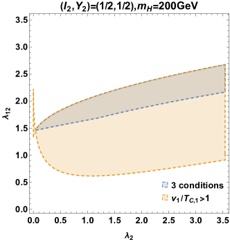
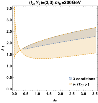
Figure 6: Comparison between the parameter region satisfying 3 conditions for two-step phase transition and SFOPT for the second step. The second region comprises the first one for both figures, with different isospins and hypercharges of $\Phi_{2}$.

5 Gravitational Wave Spectrum

Before doing numerical analysis, we briefly discuss the GW produced by the first-order phase transition. Typically, the GW spectrum from the first-order phase transition could be characterized by phase transition parameters: $T_{t}$, $\alpha$, $\beta/H$, and $v_{b}$.

The first parameter $T_{t}$ is the transition temperature that is defined by an equation that a bubble nucleation probability $\Gamma$ per Hubble volume per Hubble time reaches the unit Coleman:1977py :

$$\Gamma/H^{4}|_{T=T_{t}}=1,$$ (63)

where

$$\Gamma\simeq{\rm max}\left[T^{4}\left(\frac{S_{3}}{2\pi T}\right)^{3/2}\exp(-S_{3}/T),\,\,R_{0}^{-4}\left(\frac{S_{4}}{2\pi}\right)^{2}\exp(-S_{4})\right].$$ (64)

Here, $S_{3}$ ($S_{4}$) is a 3- (4-) dimensional Euclidean action for O(3) (O(4)) symmetric bounce solution. Also, $R_{0}$ is the size of the nucleating bubble. The Eq. (63) means one critical bubble nucleates into the causality.

The second parameter $\alpha$ is the normalized released energy density by the radiation energy density at $T_{t}$:

$$\alpha\equiv\epsilon(T_{t})/\rho_{rad}(T_{t}),$$ (65)

where $\rho_{rad}=(\pi^{2}/30)g_{*}T^{4}$ and $\epsilon$ is released energy density:

$$\epsilon(T)=\Delta V_{eff}-T\frac{\partial\Delta V_{eff}}{\partial T},\quad\Delta V_{eff}=V_{eff}(\varphi_{-}(T),T)-V_{eff}(\varphi_{+}(T),T),$$ (66)

where $\varphi_{+(-)}$ is $\varphi$ at the broken (unbroken) phase.

The third parameter $\beta/H$ is the normalized $\beta$ parameter which is related to the time variation scale of bubble nucleation rate $\Gamma(t)=\Gamma_{0}\exp(\beta t)$. This normalized $\beta$ parameter is defined as

$$\frac{\beta}{H}\equiv\left.\frac{dS_{3}}{dT}\right|_{T=T_{t}}.$$ (67)

The last one is the bubble wall velocity $v_{b}$. In our following analysis, we fix it by hand for simplicity.

By using these parameters, the GW spectrum from first-order phase transition could be estimated. There are three sources of GW spectrum: bubble collision Huber:2008hg , plasma turbulence Caprini:2009yp , and compression wave of plasma Caprini:2015zlo . The spectra could be calculated by the details of bubble dynamics, and the fitting formulas of them are provided in Ref. Caprini:2015zlo . In our analysis, we will focus on the GW spectrum from compression wave of plasma, which typically is the largest contribution among them. The formula from the compression wave of plasma Caprini:2015zlo is given by

$$\Omega_{\rm comp}(f)h^{2}=\widetilde{\Omega}_{\rm comp}h^{2}\times(f/\tilde{f}_{\rm comp})^{3}\left(\frac{7}{4+3(f/\tilde{f}_{\rm comp})^{2}}\right)^{7/2},$$ (68)

where the tilde parameters are the peak of the spectrum

$$\widetilde{\Omega}_{\rm comp}h^{2}\simeq 2.65\times 10^{-6}v_{b}\tilde{\beta}^{-1}\left(\frac{\kappa_{v}\alpha}{1+\alpha}\right)^{2}\left(\frac{100}{g_{\ast}}\right)^{1/3},$$ (69)

and the peak frequency

$$\tilde{f}_{\rm comp}\simeq 1.9\times 10^{-5}~{}{\rm Hz}\frac{1}{v_{b}}\tilde{\beta}\left(\frac{T_{t}}{100~{}{\rm GeV}}\right)\left(\frac{g_{\ast}}{100}\right)^{1/6}.$$ (70)

Here, the $g_{\ast}$ is the number of degrees of freedom in the plasma. The parameter $\kappa_{v}$ in Eq. (69) is an efficiency factor, which denotes the fraction of the vacuum energy transformed into the bulk motion of the plasma fluid Espinosa:2010hh :

$$\kappa_{v}(v_{b},\alpha)\simeq\begin{cases}&\frac{c_{s}^{11/5}\kappa_{A}\kappa_{B}}{(c_{s}^{11/5}-v_{b}^{11/5})\kappa_{B}+v_{b}c_{s}^{6/5}\kappa_{A}}\quad(\text{for}~{}v_{b}\lesssim c_{s})\\ &\kappa_{B}+(v_{b}-c_{s})\delta\kappa+\frac{(v_{b}-c_{s})^{3}}{(v_{J}-c_{s})^{3}}[\kappa_{C}-\kappa_{B}-(v_{J}-c_{s})\delta\kappa]\quad(\text{for}~{}c_{s}<v_{b}<v_{J})\\ &\frac{(v_{J}-1)^{3}v_{J}^{5/2}v_{b}^{-5/2}\kappa_{C}\kappa_{D}}{[(v_{J}-1)^{3}-(v_{b}-1)^{3}]v_{J}^{5/2}\kappa_{C}+(v_{b}-1)^{3}\kappa_{D}}\quad(\text{for}~{}v_{J}\lesssim v_{b})\end{cases},$$ (71)

where $c_{s}$ is the velocity of sound ($c_{s}=0.577$) and

$$\kappa_{A} \simeq v_{b}^{6/5}\frac{6.9\alpha}{1.36-0.037\sqrt{\alpha}+\alpha},\quad\kappa_{B}\simeq\frac{\alpha^{2/5}}{0.017+(0.997+\alpha)^{2/5}},$$

$$\kappa_{C} \simeq\frac{\sqrt{\alpha}}{0.135+\sqrt{0.98+\alpha}},\quad\kappa_{D}\simeq\frac{\alpha}{0.73+0.083\sqrt{\alpha}+\alpha}.$$ (72)

In order to discuss the testability of the parameter region for the multi-step EWPT, we estimate the signal-to-noise (S/N) ratio for measurements of GW spectrum Thrane:2013oya ; Caprini:2015zlo . The S/N ratio is defined as

$$S/N\,\,{\rm ratio}\equiv\sqrt{\delta\times t_{obs}\int^{f_{max}}_{f_{min}}df\left[\frac{h^{2}\Omega_{GW}(f)}{h^{2}\Omega_{Sens}(f)}\right]^{2}},$$ (73)

where $\delta$ is the number of independent channels for the experiment, $t_{obs}$ corresponds to the experimental observation period, $h^{2}\Omega_{GW}(f)$ denotes the GW signal coming from the first-order phase transition and $h^{2}\Omega_{Sens}(f)$ denotes the sensitivity of experiments, such as LISA Klein:2015hvg , DECIGO and BBO Yagi:2011wg . When the S/N ratio at the LISA experiment is larger than 10, we could detect the GW spectrum Caprini:2015zlo . In our analysis, we take S/N>10 as a criterion for whether the GW spectrum could be detected or not.

Supercooling phase transition

For the second step of the EWPT in Fig. 1-(b), a barrier between magenta and red points appears at zero temperature. Then, the supercooling phase transition may be realized. The condition of the supercooling phase transition is typically given as $\alpha\gg 1$. In the case of the supercooling phase transition, the broken phase may not fill with causality. Therefore we should estimate the temperature for bubble percolation for the phase transition to complete successfully. The percolation temperature $T_{p}$ means the broken phase is filled at least $34\%$ of the comoving volume at this temperature Enqvist:1991xw ; Ellis:2018mja . To evaluate the $T_{p}$, we use the probability of finding a point still in the false vacuum:

$$P(T)=e^{-I(T)},\quad I(T)=\frac{4\pi}{3}\int^{T}_{T_{c}}dT^{\prime}\Gamma(T^{\prime})a(T^{\prime})^{3}r(T,T^{\prime})^{3},$$ (74)

where $a(T^{\prime})$ is the Friedmann-Robertson-Walker scale factor, and $r(T,T^{\prime})$ is the growing comoving size of a bubble from $T^{\prime}$ to $T$:

$$r(T,T^{\prime})=\int^{t}_{t^{\prime}}\frac{d\tilde{t}v_{w}}{a(\tilde{t})}.$$ (75)

The $P(T)$ in Eq. (74) denotes the amount of true vacuum volume per unit comoving volume. By using it, the percolation temperature $T_{p}$ is defined as

$$I(T_{p})=0.34.$$ (76)

The physical volume of the false vacuum space ${\cal V}_{\rm false}$ decreases around percolation to complete the phase transition. The condition is given by Ellis:2018mja

$$\frac{1}{{\cal V}_{\rm false}}\frac{d{\cal V}_{\rm false}}{dt}<0\quad\to\quad H(T)\left(3+T\frac{dI(T)}{dT}\right)<0.$$ (77)

From this condition and equation, we can obtain the $T_{p}$. Since the bubbles for the broken phase collide with each other at this temperature, the phase transition parameters are determined at this temperature $T_{p}$. In the S/N ratio phase transition, the GW spectrum is replaced as Ellis:2018mja

$$\Omega_{\rm comp}(f)h^{2}=2.65\times 10^{-6}v_{b}\frac{H\bar{R}}{(8\pi)^{1/3}}\left(\frac{\kappa_{v}\alpha}{1+\alpha}\right)^{2}\left(\frac{100}{g_{\ast}}\right)^{1/3}(f/\tilde{f}_{\rm comp})^{3}\left(\frac{7}{4+3(f/\tilde{f}_{\rm comp})^{2}}\right)^{7/2},$$ (78)

where

$$\tilde{f}_{\rm comp}\simeq 1.9\times 10^{-5}\frac{1}{v_{b}}\frac{(8\pi)^{1/3}}{H\bar{R}}\left(\frac{T_{t}}{100~{}{\rm GeV}}\right)\left(\frac{g_{\ast}}{100}\right)^{1/6}.$$ (79)

where $\bar{R}\sim(v_{w}-c_{s})R_{\rm max}$ and $R_{\rm max}$ is the size of the bubble of maximum-energy-configuration of bubble distributions at percolation.

We will evaluate the GW spectrum from the first-order phase transition in our model by the above equations. In the following numerical results, we will obtain the phase transition parameters in the model with the EWPT in Fig. 1-(b) and will discuss the testability of the model parameters by the S/N ratio. After that, we will show whether the two first-order EWPTs could be realized or not.

6 Numerical Results

Patterns of EWPTs

According to the results in Sec. 4, the EWPT in Fig. 1-(a) and -(b) could be realized in the model, especially, multi-step EWPT in Fig. 1-(b) can occur by the red parameter region in Fig. 3. We will numerically analyze the detail of the possibility of the pattern of the EWPT in the model with $Y_{2}=1/2$ and $I_{2}=1/2$. In the numerical analysis in this section, the four parameters in the potential, $\mu_{1}^{2}$, $\mu_{2}^{2}$, $\lambda_{1}$ and $\lambda_{12}$, will be taken as $v$, $v_{2}$, $m_{h}$ and $m_{H}$ by using the stationary conditions and second derivative of the potential of Eqs. (B), (B), (B) and (B) in Appendix B. The conditions for the multi-step EWPT, which are shown in Eqs. (50), (51) and (52), are given by Fig. 7.

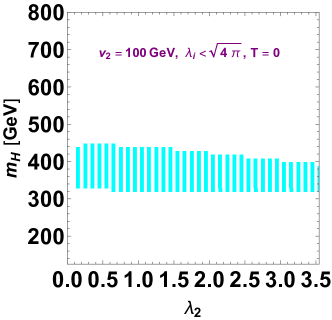
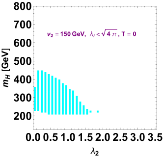
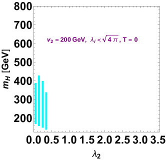
Figure 7: Regions of realizing the EWPT in Fig. 1-(a) and -(b) by the potential with one-loop effects ($Y_{2}=1/2$ and $I_{2}=1/2$). These color regions can satisfy the conditions of "Two different local minima" and "The global minimum".

These color regions can satisfy the conditions, including one-loop effects in the cases that $v_{2}=$ 100, 150, and 200 GeV. In these cyan regions, the multi-step EWPT may be generated, however, we use the potential without finite temperature effects to describe these regions. Therefore, we should consider the potential with finite temperature effects to get more detail on the possibility of the EWPTs, like the condition of "$h_{2}$ vacuum appears first when cooling down". The results, including the finite temperature effect, are given in Fig. 8.

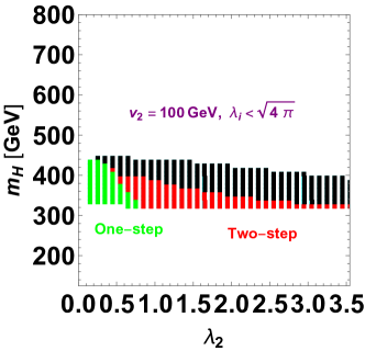
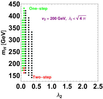
Figure 8: EWPT pattern in the plane of ($\lambda_{2}$, $m_{H}$ [GeV]) for $v_{2}=$ 100 and 200 GeV. The green squares represent the parameter region for the one-step phase transition of Fig. 1-(a). The red squares represent the parameter region for the two-step phase transition of Fig. 1-(b). In the black squares, the EWPT has not been completed in the current universe. A red star mark in the right panel could realize two first-order phase transitions in both steps of Fig. 1-(b).

To clarify the one-step and multi-step EWPT in Fig. 1-(a) and -(b), we compare the temperatures starting the phase transition along $h_{1}$ and $h_{2}$ axes. In the red (green) square marks, such a temperature along $h_{2}$ ($h_{1}$) is higher than $h_{1}$ ($h_{2}$). Furthermore, the one-step EWPT of Fig. 1-(a) (green squares) and the second step of the EWPT in Fig. 1-(b) (red squares) are first order. Since a barrier in the second path of the multi-step EWPT at red squares (one-step EWPT at green squares) occurs by the non-thermal effects (thermal effects), the frequency of GW may be different between the path of the EWPT of Fig. 1-(a) and -(b). According to the numerical results, the peak frequency at red squares is less than about $10^{-1}$ Hz, while the frequency at green squares is ${\cal O}(1)$ Hz. Therefore, we may distinguish the patterns of the EWPT of Fig. 1-(a) and -(b) by the GW observation. At the black square marks, the EWPT cannot be completed at the current universe because the barrier for the second step of the EWPT in Fig. 1-(b) does not disappear at zero temperature. At the red star mark in the right panel of Fig. 8, both steps of the EWPT in Fig. 1-(b) are first order. It is difficult to realize such a phase transition because the first step relies on finite temperature effects. The detail of that will be discussed in the following paragraph of "Possibility of two first-order EWPTs". As the numerical results in Fig. 8, the multi-step EWPT in Fig. 1-(b) could be realized in the case of the large $\lambda_{2}$ value, that can follow the condition in Eq. (53). Also, when we take heavy $m_{H}$ and large $\lambda_{2}$ value, the EWPT has not been completed, because the height difference between the magenta and blue points $\Delta V$ becomes high by heavy $m_{H}$ and the large $\lambda_{2}$: $\Delta V\sim\frac{\lambda_{2}}{4v^{4}}(2v_{2}^{2}(m_{H}^{2}+\lambda_{2}v_{2}^{2})-m_{h}^{2}v^{2})^{2}$. For example, the large $\lambda_{2}$ with $v_{2}=$ 200 GeV is prohibited by the condition of height potential in Eq. (52). These behaviors could follow the discussion in Sec. 4.

Isospin and hypercharge effects

The isospin and hypercharge of the multiplet also contribute to the patterns of the EWPT. Firstly, we note that the hypercharge of additional scalar boson $Y_{2}$ does not contribute much to the order of step of the multi-step EWPT. The effect of $Y_{2}$ appears in denominator of $T_{2}$, and it is proportional to $(m_{Z}^{2}-m_{W}^{2})$. Since the masses of these gauge bosons are almost the same, the $Y_{2}$ does not much affect the EWPT. On the other hand, the small $I_{2}$ makes the multi-step EWPT because the effect of $I_{2}^{2}$ in the denominator of $T_{2}$, which does not appear in $T_{1}$, can be neglected. Then, the $T_{2}^{2}>T_{1}^{2}$ condition can be realized. On the other hand, for the large $I_{2}$, the $T_{1}$ and $T_{2}$ are roughly given by

$$T_{1}^{2} \sim\frac{3m_{h}^{2}v^{2}}{2I_{2}(m_{H}^{2}+\lambda_{2}v_{2}^{2})},\quad T_{2}^{2}\sim\frac{\lambda_{2}v_{2}^{2}v^{2}+\frac{3I_{2}\lambda_{2}^{2}v^{2}v_{2}^{2}}{\pi^{2}}\left(\ln\frac{T_{2}^{2}\alpha_{B}}{Q^{2}}-\frac{3}{2}\right)}{I_{2}^{2}m_{W}^{2}},$$ (80)

where the second term in the $T_{2}$ is one-loop effect with the $I_{2}$ dependence. One-loop effect in the $T_{1}$ could be neglected because such a term becomes small by using the condition of the height of potential in Eq. (52): $v_{2}^{2}<m_{h}v/\sqrt{2}$. By using these terms $T_{1}$ and $T_{2}$, the ratio of these terms is

$$\frac{T_{2}^{2}}{T_{1}^{2}}\sim\frac{2\lambda_{2}(m_{H}^{2}+\lambda_{2}v_{2}^{2})v_{2}^{2}\left(1+\frac{3I_{2}\lambda_{2}}{\pi^{2}}\left(\ln\frac{T_{2}^{2}\alpha_{B}}{Q^{2}}-\frac{3}{2}\right)\right)}{3I_{2}m_{W}^{2}m_{h}^{2}}.$$ (81)

Due to this ratio, the denominator has the isospin effect, however, the $I_{2}$ dependence in this ratio disappears when the last term in the numerator is large. Then the value of $\lambda_{2}$ is an important source to realize the two-step phase transition. For the heavy $m_{H}$ case, the $T_{2}^{2}/T_{1}^{2}$ ratio is roughly given by

$$\frac{T_{2}^{2}}{T_{1}^{2}}\sim\frac{\lambda_{2}v_{2}^{2}(1+2I_{2})+\frac{3m_{h}^{2}}{2\pi^{2}}\left(\ln\frac{T_{2}^{2}\alpha_{B}}{Q^{2}}-\frac{3}{2}\right)}{m_{h}^{2}}.$$ (82)

In this case, the $I_{2}$ is important to realize the two-step phase transition.

The numerical results of the isospin dependence are given by Fig. 9.

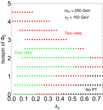
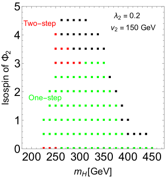
Figure 9: The isospin dependences of the EWPT patterns. The Left figure is the dependence for $\lambda_{2}$ with $m_{H}$ = 250 GeV and $v_{2}$ = 150 GeV. The right figure is the dependence for $m_{H}$ with $\lambda_{2}$ = 0.2 and $v_{2}$ = 150 GeV. Otherwise, the same as Fig. 8.

The horizontal axis is the left (right) figure is $\lambda_{2}$ ($m_{H}$), and the vertical axes are $I_{2}$. In the black squares, the EWPT is multi-step and has not been completed in the current universe. According to these figures, the multi-step EWPT could be generated by the large $\lambda_{2}$. Furthermore, the small or large $I_{2}$ value is the source of the multi-step EWPT. These results could follow the above discussion. From that, we can find that the EWPT can assure the $Z_{2}$ symmetry after the spontaneous EWSB in the model with $I_{2}<5$.

The Collider Constraints

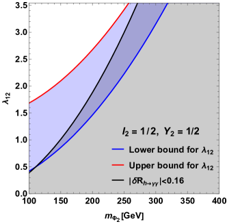
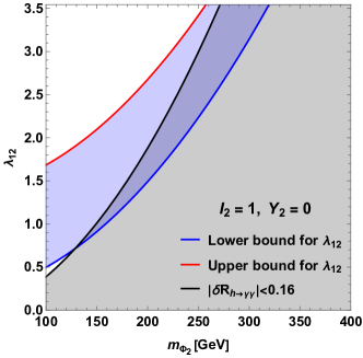
Figure 10: The condition of two-step phase transition and $h\gamma\gamma$ measurement in the plane of ($m_{\Phi_{2}}$, $\lambda_{12}$) in the model with ($I_{2}$, $Y_{2}$)=(1/2,1/2) and (1,0). The condition of a two-step phase transition can be realized in the blue region. The black region is allowed by the $h\gamma\gamma$ measurements.

Although the multiplet carries the $Z_{2}$ symmetry, which forbids the mixing between the neutral scalar component and the SM Higgs boson, there are still constraints on the model parameters. At the LHC, the Drell-Yan process produces a pair of the charged components of the multiple, and the charged scalar subsequently decays into the SM weak gauge bosons and the neutral scalar. Thus the charged scalars have been tightly constrained except that the charged scalars and neutral scalars have degenerate masses ATLAS:2015eiz . So in the following, we focus on the multiplet in which all the components have degenerate masses . Furthermore, we also assume that the neutral scalar only contributes to part of the relic abundance, so the constraints from the relic density could be avoided.

One unavoidable constraint from the loop correction is the constraints from the $h\to\gamma\gamma$ measurements at the LHC. The deviation from the SM prediction in the $h\to\gamma\gamma$ is given by

$$\delta R_{h\to\gamma\gamma}=\frac{\Gamma_{h\to\gamma\gamma}^{\rm SM+BSM}-\Gamma_{h\to\gamma\gamma}^{\rm SM}}{\Gamma_{h\to\gamma\gamma}^{\rm SM}},$$ (83)

where the $\Gamma_{h\to\gamma\gamma}^{\rm SM+BSM}$ is the decay rate of $h\to\gamma\gamma$ in this model, which is given by Ramsey-Musolf:2021ldh

$$\Gamma_{h\to\gamma\gamma}^{\rm SM+BSM}=\frac{v^{2}\alpha_{e}^{2}m_{h}^{3}}{256\pi^{3}}\left|\frac{4}{3}A_{1/2}\left(\frac{4m_{t}^{2}}{m_{h}^{2}}\right)+A_{1}\left(\frac{4m_{W}^{2}}{m_{h}^{2}}\right)+\sum_{n=-I_{2}}^{I_{2}}\frac{\lambda_{12}v^{2}}{2m_{\Phi_{2}}^{2}}\left(n+Y_{2}\right)A_{1}\left(\frac{4m_{\Phi_{2}}}{m_{h}^{2}}\right)\right|^{2}$$ (84)

where $\alpha_{e}=e^{2}/4\pi$the loop function $A_{1/2}$, $A_{1}$ and $A_{0}$ is defined as Chen:2013vi

$$A_{1}(\tau) =2+3\tau+3\tau(2-\tau)f(\tau),$$ (85)

$$A_{\frac{1}{2}}(\tau) =-2\tau\left\{1+(1-\tau)f(\tau)\right\},$$ (86)

$$A_{0}(\tau) =\tau\left(1-\tau f(\tau)\right)$$ (87)

with

$$f(\tau)=\left\{\begin{array}[]{ll}\arcsin^{2}\sqrt{1/\tau}&\quad\tau\geq 1\\ -\frac{1}{4}\left(\ln\frac{1+\sqrt{1-\tau}}{1-\sqrt{1-\tau}}-i\pi\right)&\quad\tau<1\\ \end{array}\right..$$ (90)

The current bound for the effective coupling of the Higgs boson to the photon $\kappa_{\gamma}$ is $1.02^{+0.16}_{-0.14}$ at 95$\%$ confidence level ATLAS:2022tnm . Fig. 10 represents the condition of two-step phase transition and the $h\gamma\gamma$ observation in the plane of ($m_{\Phi_{2}}$, $\lambda_{12}$). $m_{\Phi_{2}}$ is the degenerate mass of additional charged-scalar bosons. The left and right panels are the results in the model with ($I_{2}$, $Y_{2}$)=(1/2,1/2) and (1,0), respectively. The blue region can satisfy the conditions of a two-step phase transition. The black region is allowed region with $|\delta R_{h\to\gamma\gamma}|<0.16$. Due to this figure, the two-step phase transition can be realized in the allowed region for $h\gamma\gamma$ observation. The numerical results in Figs. 8 and 9 can be avoided the current bound of $h\to\gamma\gamma$ observation.

First-order phase transition and GW Signatures

In this part, we will show the testability of the parameter region of the left panel of Fig. 8. Fig. 11 represents the results of the S/N ratio, which is given by in Eq. (73), of the green and red squares in the left panel of Fig. 8. The left (right) two figures represent the S/N ratio for LISA Klein:2015hvg (BBO Yagi:2011wg ). The experimental period for the S/R ratio is chosen as 5 years. The red dashed line in these figures represents $S/N=10$. The parameter regions above the red dashed line can realize $S/N>10$. Therefore, such a parameter region can be tested by each experiment.

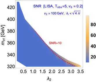
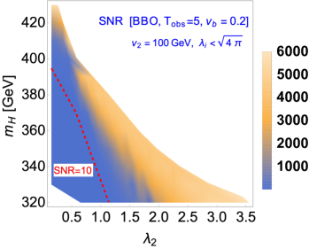
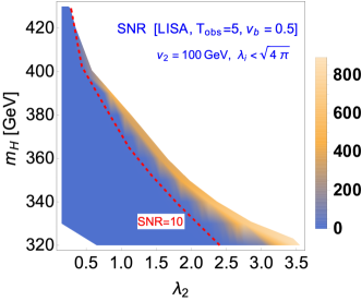
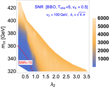
Figure 11: The density plots of $S/N$ ratio at LISA (left two figures) and BBO (right two figures) experiments. The experimental period is chosen as 5 years. The top (bottom) two figures have $v_{b}$=0.2 (0.5), respectively. The red dashed lines in these figures represent $S/N=10$.

The top (bottom) two figures have $v_{b}$ = 0.2 (0.5), respectively. The low speed of bubble wall velocity is required to generate the baryon asymmetry of the universe Joyce:1994fu . The upper right parts of the white regions in these figures correspond to the black squares in Fig. 8, which represent that the EWPT has not been completed in the current universe. The parameter region close to the upper right white region can be tested at the LISA. On the other hand, the BBO can test the almost parameter region realizing, especially the multi-step EWPT in Fig. 1-(b). Therefore, we can use the GW observation experiments to explore the possibility of the multi-step EWPT to restore the $Z_{2}$ symmetry after the spontaneous EWSB.

The first-order EWPT in Fig. 1-(a) can be realized by the negative $\mu_{2}^{2}$ case. However, the first-order phase transition is not strong enough to generate the detectable GW spectrum because the $\lambda_{12}v^{2}$ is typically smaller for negative $\mu_{2}^{2}$ than for positive $\mu_{2}^{2}$ to determine the $m_{H}$.

Possibility of two first-order EWPTs

For the red star point in Fig. 8 with $v_{2}=200~{}{\rm GeV}$, the two peaks of GW spectra could be produced by the two first-order phase transitions in (green $\to$ magenta) and (magenta $\to$ red) paths, depicted in Fig. 5. Parameters at the red star point are $(v_{2},m_{H},\lambda_{2},I_{2},Y_{2})$ = (200 GeV, 180 GeV, 0.08, 1/2, 1/2). The GW spectra of this parameter are shown by Fig. 12-(1). The red (black) lines are the GW spectrum from the first-step (second-step) EWPT in Fig. 1-(b). The phase transition parameters are $(T_{t},\alpha,\tilde{\beta},v_{b})=$ (149 GeV, $3.79\times 10^{-4},8.37\times 10^{5}$, 0.5) [first step] and (142 GeV, $4.70\times 10^{-3},4.91\times 10^{3}$, 0.5) [second step]. The blue and yellow lines correspond to the sensitivity of the LISA and BBO experiments, respectively. The S/N ratio for these spectra are given as $S/N$ (LISA) $\sim 10^{-16}$, $S/N$ (BBO) $\sim 10^{-7}$ [first step] and $S/N$ (LISA) $\sim 10^{-7}$, $S/N$ (BBO) $\sim 0.565$ [second step]. Therefore, it could not be easy to detect these GW spectra in Fig. 12-(1). On the other hand, we take the second benchmark point with larger $v_{2}$ than the star point: $v_{2}=223$ GeV.

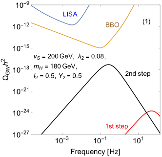
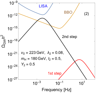
Figure 12: Examples of two peaks of GW spectrum from compression wave of plasma with $v_{b}=0.5$ and $(m_{H},\lambda_{2},I_{2},Y_{2})$ = (180 GeV, 0.08, 1/2, 1/2). (1) Left figure is two peaks of GW spectra at the red star point in the right panel of Fig. 8, which has $v_{2}$ = 200 GeV. (2) Right figure is the spectra about $v_{2}$ = 223 GeV. The red (black) GW spectrum comes from the first-step (second-step) EWPT in Fig. 1-(b). The blue and yellow lines are the sensitivity lines at LISA and BBO, respectively.

The GW for the second benchmark point is described in Fig. 12-(2), and the phase transition parameters are $(T_{t},\alpha,\tilde{\beta},v_{b})=$ (153 GeV, $5.03\times 10^{-4},9.58\times 10^{4}$, 0.5) [first step] and (109 GeV, $3.06\times 10^{-2}$, 72.2, 0.5) [second step]. The S/N ratio for each path in Fig. 12-(2) are $S/N$ (LISA) $\sim 10^{-16}$, $S/N$ (BBO) $\sim 10^{-9}$ [first step] and $S/N$ (LISA) $\sim$ 58.0, $S/N$ (BBO) $\sim$ 238 [second step]. Therefore, we could detect one peak of GW spectrum at least. However, these experiments are difficult to observe both GW spectra from the two first-order EWPTs in Fig. 1-(b). The reasons why the GW spectrum from the first step is so small are (i) first-step EWPT does not have non-thermal contributing to cubic term $h_{2}^{3}$, and (ii) $\lambda_{2}$ could not be small enough to generate the strongly first-order EWPT. The detectable GW spectrum could require a large value of $v_{C}/T_{C}$; in other words, it could require a small value of $\lambda_{2}$. However, the condition of $T_{2}>T_{1}$ in Eq. (53) cannot be satisfied by such a small value of $\lambda_{2}$. In the case of large $v_{2}$ value, multi-step phase transitions are realized even for small values of $\lambda_{2}$, and two first-order EWPTs may be realized. But the condition of the height of the potential between the magenta and red points in Fig. 2 becomes strict by the large $v_{2}$: $\lambda_{2}v_{2}^{4}<m_{h}^{2}v^{2}/2$. Therefore, the parameter region for producing the detectable two peaks of the GW spectrum is very narrow.

Furthermore, we study the supercooling phase transition ($\alpha\gg 1$). The benchmark point of the supercooling phase transition is $(v_{2},m_{H},\lambda_{2},I_{2},Y_{2})$ = (225 GeV, 168.64 GeV, 0.08, 1/2, 1/2). Then the percolation temperature of the second path is $T_{p}\sim 4$ GeV, and $\alpha\sim 3880$. However, even in the supercooling case, the first step of the EWPT is not strong. It is difficult to detect both peaks of the GW spectra coming from both steps of the EWPT in Fig. 1-(b); however, at least one peak of the spectra could be detected. Suppose the multi-step EWPT is unable to restore the $Z_{2}$ symmetry after the spontaneous EWSB, e.g., Fig. 1-(e) phase transition. In that case, we could detect both peaks of GW spectra produced by two first-order EWPTs Aoki:2021oez , because the condition of the height of the potential is not necessary to realize the multi-step EWPT.

7 Summary

We have investigated that the two-step phase transition can be naturally realized in the scalar potential with the discrete $Z_{2}$ symmetry due to degenerate extreme along field directions. To lay out the general conditions on such a two-step phase transition, we consider the most general electroweak $N$-plet scalar extension. For the first time, we provide the general form of the Deybe masses and obtain the two-step phase transition conditions for general isospin and hypercharge scalars. We found that there is a strong correlation between the coupling $\lambda_{12}$ and the heavy scalar mass, and the coupling $\lambda_{12}$ needs to be in a moderate region because of the global minimum and $T_{2}>T_{1}$ conditions. As the heavy scalar mass increase, the coupling $\lambda_{12}$ is required to take a larger value, and similarly for larger isospin multiplet.

Although both steps of the EWPT could be first-order, it is difficult to detect two peaks of GW spectra produced from these first-order EWPTs. The first-order EWPT along the first step can be realized by thermal loop effects, and then typically, the GW spectrum frequency is ${\cal O}(1)$ Hz. The detectable GW spectrum from this step can be produced if there is a small $\lambda_{2}$ or large $v_{2}$ value. Since a barrier in the second step of the EWPT occurs by the tree-level effects, the detectable GW could be generated through the second step, of which the frequency is less than about $10^{-1}$ Hz. Therefore, we may distinguish different patterns of the EWPT by the GW observation.

Even in the case that the multi-step EWPT is able to restore the discrete symmetry, at least one peak of the spectrum could be detected by future GW observation experiments. According to the numerical results, the second step produces the GW spectrum that could be detected in the BBO experiment. Furthermore, it is possible to explore such parameter region of the moderately large $\lambda_{12}$ by the Higgs diphoton data in future hadron and lepton colliders. From these experiments, we would explore the possibility of multi-step phase transition comprehensively.

Appendix A Field-dependent masses in several multiplets

The field-dependent mass (matrix) can be calculated by taking the second derivatives of the potential as

$$M_{ij}^{2}(h_{1},h_{2})=\frac{\partial^{2}V_{0}}{\partial\phi_{i}\partial\phi_{j}}\Bigg{|}_{h_{1},h_{2}},$$ (91)

where $\phi$ can be scalars, fermions, and gauge bosons. We list the mass matrix squared under various representations $(I_{2},Y_{2})$ as following:

Notation

• NS, CS, and NCPC are abbreviations of neutral scalar, charged scalar, and neutral CP conserving scalar. By default, $n_{\text{NS}}=n_{\text{NCPC}}=1,~{}n_{\text{CS}}=2$.

• $\chi$ is components of $\Phi_{1}$ except $h_{1}$. By default, $n_{\chi}=3$.

• $c^{+}=2\operatorname{Re}(c)=c+c^{*},~{}c^{-}=2\operatorname{Im}(c)=-i(c-c^{*})$ for parameter c.

Real singlet

$(0,0)$:

$$M_{\rm{NS}}^{2} =\left(\begin{array}[]{cc}3\lambda_{1}h_{1}^{2}+a_{0}h_{2}^{2}-\mu_{1}^{2}&2a_{0}h_{1}h_{2}\\ 2a_{0}h_{1}h_{2}&12b_{0}h_{2}^{2}+a_{0}h_{1}^{2}-\mu_{2}^{2}\end{array}\right),$$ (94)

$$M_{\chi}^{2} =\lambda_{1}h_{1}^{2}+a_{0}h_{2}^{2}-\mu_{1}^{2}.$$ (95)

Complex singlet

$(0,0)$:

$$M_{\rm{NS}}^{2} =\left(\begin{array}[]{ccc}(M_{\rm{NS}}^{11})^{2}&(a_{0}+a_{1}^{\prime+})h_{1}h_{2}&-a_{0}^{\prime-}h_{1}h_{2}\\ (a_{0}+a_{1}^{\prime+})h_{1}h_{2}&(M_{\rm{NS}}^{22})^{2}&-\frac{1}{2}a_{0}^{\prime-}h_{1}^{2}-3\left(b_{0}^{\prime-}+\frac{1}{2}b_{0}^{\prime\prime-}\right)h_{2}^{2}\\ -a_{0}^{\prime-}h_{1}h_{2}&-\frac{1}{2}a_{0}^{\prime-}h_{1}^{2}-3\left(b_{0}^{\prime-}+\frac{1}{2}b_{0}^{\prime\prime-}\right)h_{2}^{2}&(M_{\rm{NS}}^{aa}))^{2}\end{array}\right),$$ (99)

$$M_{\chi}^{2} =\lambda_{1}h_{1}^{2}+\frac{1}{2}a_{0}h_{2}^{2}-\mu_{1}^{2},$$ (100)

where

$$(M_{\rm{NS}}^{11})^{2} =3\lambda_{1}h_{1}^{2}+\frac{1}{2}(a_{0}+a_{1}^{\prime+})h_{2}^{2}-\mu_{1}^{2},$$

$$(M_{\rm{NS}}^{22})^{2} =3(b_{0}+b_{0}^{\prime+}+b_{0}^{\prime\prime+})h_{2}^{2}+\frac{1}{2}(a_{0}+a_{1}^{\prime+})h_{1}^{2}-\mu_{2}^{2},$$

$$(M_{\rm{NS}}^{aa})^{2} =(b_{0}-3b_{0}^{\prime+})h_{2}^{2}+\frac{1}{2}(a_{0}-a_{0}^{+})h_{1}^{2}-\mu_{2}^{2}.$$ (101)

Doublet

$(1/2,1/2)$:

$$M_{\rm{NS}}^{2} =\left(\begin{array}[]{cccc}(M_{\rm{NS}}^{11})^{2}&(a_{0}+a_{1}^{\prime+})h_{1}h_{2}&-\frac{1}{2}a_{1}^{\prime-}h_{2}^{2}&a_{1}^{\prime-}h_{1}h_{2}\\ (a_{0}+a_{1}^{\prime+})h_{1}h_{2}&(M_{\rm{NS}}^{22})^{2}&-a_{1}^{\prime-}h_{1}h_{2}&\frac{1}{2}a_{1}^{\prime-}h_{1}^{2}\\ -\frac{1}{2}a_{1}^{-}h_{2}^{2}&-a_{1}^{-}h_{1}h_{2}&(M_{\rm{NS}}^{\phi_{0}\phi_{0}})^{2}&a_{1}^{\prime+}h_{1}h_{2}\\ a_{1}^{\prime-}h_{1}h_{2}&\frac{1}{2}a_{1}^{\prime-}h_{1}^{2}&a_{1}^{\prime+}h_{1}h_{2}&(M_{\rm{NS}}^{aa})^{2}\end{array}\right),$$ (106)

$$M_{\rm{CS}}^{2} =\left(\begin{array}[]{cc}\lambda_{1}h_{1}^{2}+\frac{1}{2}(a_{0}+a_{1})h_{2}^{2}-\mu_{1}^{2}&-\frac{1}{2}(a_{1}-2a_{1}^{\prime})h_{1}h_{2}\\ -\frac{1}{2}(a_{1}-2a_{1}^{\prime*})h_{1}h_{2}&b_{0}h_{2}^{2}+\frac{1}{2}(a_{0}+a_{1})h_{1}^{2}-\mu_{2}^{2}\end{array}\right),$$ (108)

where

$$(M_{\rm{NS}}^{11})^{2} =3\lambda_{1}h_{1}^{2}+\frac{1}{2}(a_{0}+a_{1}^{\prime+})h_{2}^{2}-\mu_{1}^{2},$$

$$(M_{\rm{NS}}^{22})^{2} =3b_{0}h_{2}^{2}+\frac{1}{2}(a_{0}+a_{1}^{\prime+})h_{1}^{2}-\mu_{2}^{2},$$

$$(M_{\rm{NS}}^{\phi_{0}\phi_{0}})^{2} =\lambda_{1}h_{1}^{2}+\frac{1}{2}(a_{0}-a_{1}^{\prime+})h_{2}^{2}-\mu_{1}^{2},$$

$$(M_{\rm{NS}}^{aa})^{2} =b_{0}h_{2}^{2}+\frac{1}{2}(a_{0}-a_{1}^{\prime+})h_{1}^{2}-\mu_{2}^{2}.$$ (109)

Real triplet

$(1,0)$:

$$M_{\rm{NCPC}}^{2} =\left(\begin{array}[]{cc}3\lambda_{1}h_{1}^{2}-a_{0}h_{2}^{2}-\mu_{1}^{2}&-2a_{0}h_{1}h_{2}\\ -2a_{0}h_{1}h_{2}&12b_{0}h_{2}^{2}-a_{0}h_{1}^{2}+\mu_{2}^{2}\end{array}\right),$$ (112)

$$M_{\chi}^{2} =\lambda_{1}h_{1}^{2}-a_{0}h_{2}^{2}-\mu_{1}^{2},$$

$$M_{a}^{2} =4b_{0}h_{2}^{2}-a_{0}h_{1}^{2}+\mu_{2}^{2},~{}n_{a}=2.$$ (113)

Complex triplet

$(1,0)$:

$$M_{\rm{NS}}^{2} =\left(\begin{array}[]{ccc}(M_{\rm{NS}}^{11})^{2}&\frac{1}{2}(2a_{0}+a_{1}-2a_{0}^{\prime+})h_{1}h_{2}&a_{0}^{\prime-}h_{1}h_{2}\\ \frac{1}{2}(2a_{0}+a_{1}-2a_{0}^{\prime+})h_{1}h_{2}&(M_{\rm{NS}}^{22})^{2}&\frac{1}{2}a_{0}^{\prime-}h_{1}^{2}-3(b_{0}^{\prime-}-b_{0}^{\prime\prime-})h_{2}^{2}\\ a_{0}^{\prime-}h_{1}h_{2}&\frac{1}{2}a_{0}^{\prime-}h_{1}^{2}-3(b_{0}^{\prime-}-b_{0}^{\prime\prime-})h_{2}^{2}&(M_{\rm{NS}}^{aa})^{2}\end{array}\right),$$ (117)

$$M_{\rm{CS}}^{2} =\left(\begin{array}[]{ccc}(M_{\rm{CS}}^{G^{\pm}})^{2}&-\frac{1}{2\sqrt{2}}a_{1}h_{1}h_{2}&-\frac{1}{2\sqrt{2}}a_{1}h_{1}h_{2}\\ -\frac{1}{2\sqrt{2}}a_{1}h_{1}h_{2}&(M_{\rm{CS}}^{s^{+}})^{2}&a_{0}^{\prime}h_{1}^{2}-(b_{1}+2b_{0}^{\prime}-b_{0}^{\prime\prime})h_{2}^{2}\\ -\frac{1}{2\sqrt{2}}a_{1}h_{1}h_{2}&a_{0}^{\prime}h_{1}^{2}-(b_{1}+2b_{0}^{\prime}-b_{0}^{\prime\prime})h_{2}^{2}&(M_{\rm{CS}}^{s^{-}})^{2}\end{array}\right),$$ (121)

$$M_{G^{0}}^{2} =\lambda_{1}h_{1}^{2}+\frac{1}{4}(2a_{0}+a_{1}-2a_{1}^{\prime+})h_{2}^{2}-\mu_{1}^{2},~{}n_{G^{0}}=1,$$ (122)

where

$$(M_{\rm{NS}}^{11})^{2} =3\lambda_{1}h_{1}^{2}+\frac{1}{4}(2a_{0}+a_{1}-2a_{0}^{\prime+})h_{2}^{2}-\mu_{1}^{2},$$

$$(M_{\rm{NS}}^{22})^{2} =3(b_{0}+b_{1}+b_{0}^{\prime+}-b_{0}^{\prime\prime+})h_{2}^{2}+\frac{1}{4}(2a_{0}+a_{1}-2a_{0}^{\prime+})h_{1}^{2}-\mu_{2}^{2},$$

$$(M_{\rm{NS}}^{aa})^{2} =(b_{0}+b_{1}-3b_{0}^{\prime+})h_{2}^{2}+\frac{1}{4}(2a_{0}+a_{1}+2a_{0}^{\prime+})h_{1}^{2}-\mu_{2}^{2},$$

$$(M_{\rm{NS}}^{G^{\pm}})^{2} =M_{G^{0}},$$

$$(M_{\rm{NS}}^{s^{+}})^{2} =\frac{1}{2}(2b_{0}-b_{0}^{\prime\prime+})h_{2}^{2}+\frac{1}{2}(a_{0}+a_{1})h_{1}^{2}-\mu_{2}^{2},$$

$$(M_{\rm{NS}}^{s^{-}})^{2} =\frac{1}{2}(2b_{0}-b_{0}^{\prime\prime+})h_{2}^{2}+\frac{1}{2}a_{0}h_{1}^{2}-\mu_{2}^{2}.$$ (123)

Complex triplet

$(1,1)$:

$$M_{\rm{NCPC}}^{2} =\left(\begin{array}[]{cc}3\lambda_{1}h_{1}^{2}+\frac{1}{2}a_{0}h_{2}^{2}-\mu_{1}^{2}&a_{0}h_{1}h_{2}\\ a_{0}h_{1}h_{2}&3b_{0}h_{2}^{2}+\frac{1}{2}a_{0}h_{1}^{2}-\mu_{2}^{2}\end{array}\right),$$ (126)

$$M_{G^{0}}^{2} =\lambda_{1}h_{1}^{2}+\frac{1}{2}a_{0}h_{2}^{2}-\mu_{1}^{2},~{}n_{G^{0}}=1,$$

$$M_{a}^{2} =b_{0}h_{2}^{2}+\frac{1}{2}a_{0}h_{1}^{2}-\mu_{2}^{2},~{}n_{a}=1,$$

$$M_{\rm{CS}}^{2} =\left(\begin{array}[]{cc}\lambda_{1}h_{1}^{2}+\frac{1}{2}(a_{0}+a_{1})h_{2}^{2}-\mu_{1}^{2}&-\frac{1}{2\sqrt{2}}a_{0}h_{1}h_{2}\\ -\frac{1}{2\sqrt{2}}a_{0}h_{1}h_{2}&b_{0}h_{2}^{2}+\frac{1}{4}(2a_{0}+a_{1})h_{1}^{2}-\mu_{2}^{2}\end{array}\right),$$ (128)

$$M_{{s^{\pm\pm}}}^{2} =(b_{0}+2b_{1})h_{2}^{2}+\frac{1}{2}(a_{0}+a_{1})h_{1}^{2}-\mu_{2}^{2},~{}n_{s^{\pm\pm}}=2.$$ (129)

Appendix B Stationary conditions and neutral scalar masses

We modify the tree-level conditions in Fig. 48 by using the effective potential with the loop correction at zero temperature in Eq. (23), with the non-diagonal terms neglected. We take $Q=v=246$ GeV and the tadpole conditions are defined as follows:

$$\left.\frac{\partial V_{\rm eff}}{\partial\left\langle\Phi_{1}\right\rangle}\right|_{\left\langle\Phi_{1}\right\rangle=v,\left\langle\Phi_{2}\right\rangle=0} =-\mu_{1}^{2}+\lambda_{1}v^{2}+\frac{1}{16\pi^{2}}\Bigg{[}\frac{6\lambda_{1}+\lambda_{12}}{4}f_{+}(m_{\Phi_{1,r}}^{2},m_{\Phi_{2,r}}^{2})+\frac{1}{4}(6\lambda_{1}-\lambda_{12})f_{-}(m_{\Phi_{1,r}}^{2},m_{\Phi_{2,r}}^{2})$$

$$\quad+(2(2I_{2}-1)-1)\frac{\lambda_{12}m_{N_{2,r}}^{2}}{2}\left(\ln\frac{m_{N_{2,r}}^{2}}{Q^{2}}-1\right)+\frac{6m_{W}^{4}}{v^{2}}\left(\ln\frac{m_{W}^{2}}{Q^{2}}-\frac{1}{3}\right)$$

$$\quad+\frac{3m_{Z}^{4}}{v^{2}}\left(\ln\frac{m_{Z}^{2}}{Q^{2}}-\frac{1}{3}\right)-\frac{12m_{t}^{4}}{v^{2}}\left(\ln\frac{m_{t}^{2}}{Q^{2}}-1\right)\Bigg{]}=0,$$ (130)

$$\left.\frac{\partial V_{\rm eff}}{\partial\left\langle\Phi_{2}\right\rangle}\right|_{\left\langle\Phi_{1}\right\rangle=0,\left\langle\Phi_{2}\right\rangle=v_{2}} =-\mu_{2}^{2}+\lambda_{2}v_{2}^{2}+\frac{1}{16\pi^{2}}\Bigg{[}\frac{6\lambda_{2}+\lambda_{12}}{4}f_{+}\left((m_{\Phi_{1,b}})^{2},(m_{\Phi_{2,b}})^{2}\right))$$

$$\quad+\frac{1}{4}(\lambda_{12}-6\lambda_{2})f_{-}\left((m_{\Phi_{1,b}})^{2},(m_{\Phi_{2,b}})^{2}\right)+3\frac{\lambda_{12}}{2}(m_{N_{1,b}}^{s})^{2}\left(\ln\frac{(m_{N_{1,b}})^{2}}{Q^{2}}-1\right)$$

$$\quad+(2(2I_{2}-1)-1)\lambda_{2}(m_{N_{2,b}})^{2}\left(\ln\frac{(m_{N_{2,b}})^{2}}{Q^{2}}-1\right)$$

$$\quad+\frac{3Y_{2}^{4}m_{Z}^{4}v_{2}^{2}}{v^{4}}\left(\ln\frac{Y_{2}^{2}v_{2}^{2}m_{Z}^{2}}{Q^{2}v^{2}}-\frac{1}{3}\right)+\frac{6I_{W}^{4}m_{W}^{4}v_{2}^{2}}{v^{4}}\left(\ln\frac{I_{W}^{2}m_{W}^{2}v_{2}^{2}}{v^{2}Q^{2}}-\frac{1}{3}\right)\Bigg{]}=0,$$ (131)

where

$$f_{\pm}(m_{i}^{2},m_{j}^{2}) =m_{i}^{2}\left(\ln\frac{m_{i}^{2}}{Q^{2}}-1\right)\pm m_{j}^{2}\left(\ln\frac{m_{j}^{2}}{Q^{2}}-1\right),$$ (132)

$$\Delta m_{\Phi}^{2} =m_{\Phi_{2}}^{2}-m_{\Phi_{1}}^{2}=\sqrt{\left({\cal M}_{\Phi_{1}\Phi_{1}}^{2}-{\cal M}_{\Phi_{2}\Phi_{2}}^{2}\right)^{2}+4{\cal M}_{\Phi_{1}\Phi_{2}}^{4}},$$ (133)

$$\mathcal{M}_{h,H}^{2} =\left(\begin{array}[]{ccc}{\cal M}_{\Phi_{1}\Phi_{1}}^{2}&{\cal M}_{\Phi_{1}\Phi_{2}}^{2}\\ {\cal M}_{\Phi_{2}\Phi_{1}}^{2}&{\cal M}_{\Phi_{2}\Phi_{2}}^{2}\end{array}\right),$$ (136)

and

$$m_{\Phi_{1,r}}^{2} =-\mu_{1}^{2}+3\lambda_{1}v^{2}, m_{\Phi_{2,r}}^{2}=-\mu_{2}^{2}+\lambda_{12}v^{2}/2,$$

$$m_{N_{1,r}}^{2} =-\mu_{1}^{2}+\lambda_{1}v^{2}, m_{N_{2,r}}^{2}=-\mu_{2}^{2}+\lambda_{12}v^{2}/2,$$

$$m_{\Phi_{1,b}}^{2} =-\mu_{1}^{2}+\lambda_{12}v_{2}^{2}/2, m_{\Phi_{2,b}}^{2}=-\mu_{2}^{2}+3\lambda_{2}v_{2}^{2},$$

$$m_{N_{1,b}}^{2} =-\mu_{1}^{2}+\lambda_{12}v_{2}^{2}/2, m_{N_{2,b}}^{2}=-\mu_{2}^{2}+\lambda_{2}v_{2}^{2}/2.$$ (137)

To replace the Higgs boson mass $m_{h}$ and additional neutral CP-even boson mass $m_{H}$, we use the following second derivative of the effective potentials:

$$m_{h}^{2}\equiv\left.\frac{\partial^{2}V_{\rm eff}}{\partial\left\langle\Phi_{1}\right\rangle^{2}}\right|_{\left\langle\Phi_{1}\right\rangle=v,\left\langle\Phi_{2}\right\rangle=0} =2\lambda_{1}v^{2}+\frac{v^{2}}{32\pi^{2}}\Bigg{[}A^{r}_{2}\ln\frac{m_{\Phi_{1,r}}^{2}m_{\Phi_{2,r}}^{2}}{Q^{4}}-A^{r}_{3}\ln\frac{m_{\Phi_{1,r}}^{2}}{m_{\Phi_{2,r}}^{2}}$$

$$\quad+12\lambda_{1}^{2}\ln\frac{m_{N_{1,r}}^{2}}{Q^{2}}+4\lambda_{12}^{2}(2(2I_{2}-1)-1)\ln\frac{m_{N_{2,r}}^{2}}{Q^{2}}+12\frac{m_{Z}^{4}}{v^{4}}\left(\ln\frac{m_{Z}^{2}}{Q^{2}}+\frac{2}{3}\right)$$

$$\quad+24\frac{m_{W}^{4}}{v^{4}}\left(\ln\frac{m_{W}^{2}}{Q^{2}}+\frac{2}{3}\right)-48\frac{m_{t}^{4}}{v^{4}}\ln\frac{m_{t}^{2}}{Q^{2}}\Bigg{]}$$ (138)

$$m_{H}^{2}\equiv\left.\frac{\partial^{2}V_{\rm eff}}{\partial\left\langle\Phi_{2}\right\rangle^{2}}\right|_{\left\langle\Phi_{1}\right\rangle=v,\left\langle\Phi_{2}\right\rangle=0} =-\mu_{2}^{2}+\lambda_{12}v^{2}+\frac{1}{64\pi^{2}}\Bigg{[}B_{1}f_{-}(m_{\Phi_{2,r}}^{2},m_{\Phi_{1,r}}^{2})+B_{2}f_{+}(m_{\Phi_{2,r}}^{2},m_{\Phi_{1,r}}^{2})$$

$$\quad+4(2(2I_{2}-1)-1)\lambda_{2}m_{N_{2,r}}^{2}\left(\ln\frac{m_{N_{2,r}}^{2}}{Q^{2}}-1\right)+12\frac{m_{Z}^{4}Y_{2}^{2}}{v^{2}}\left(\ln\frac{m_{Z}^{2}}{Q^{2}}-\frac{1}{3}\right)$$

$$\quad+24\frac{m_{W}^{4}I_{W}^{2}}{v^{2}}\left(\ln\frac{m_{W}^{2}}{Q^{2}}-\frac{1}{3}\right)\Bigg{]},$$ (139)

where

$$A^{r}_{2} =\frac{1}{4}\left((6\lambda_{1}+\lambda_{12})^{2}+(6\lambda_{1}-\lambda_{12})^{2}\right),\quad A^{r}_{3}=-\frac{36\lambda_{1}^{2}-\lambda_{12}^{2}}{2}$$ (140)

$$B_{1} =\frac{2}{\Delta m^{2}}\left[\left(-6\lambda_{2}+\lambda_{12}\right)\left({\cal M}_{\Phi_{1}\Phi_{1}}^{2}-{\cal M}_{\Phi_{2}\Phi_{2}}^{2}\right)+4\lambda_{12}^{2}v^{2}\right]$$ (141)

$$B_{2} =6\lambda_{2}+\lambda_{12}.$$ (142)

The model parameters can be replaced by Eqs. (B), (B) and (B):

$$(\mu_{1}^{2},\mu_{2}^{2},\lambda_{1},\lambda_{2},\lambda_{12})\to(v,v_{2},m_{h},\lambda_{2},m_{\Phi_{2}}^{2}).$$ (143)

References

- (1) V. Kuzmin, V. Rubakov and M. Shaposhnikov, Phys. Lett. B 155 (1985), 36 doi:10.1016/0370-2693(85)91028-7
- (2) A. D. Sakharov, Pisma Zh. Eksp. Teor. Fiz. 5, 32 (1967) [JETP Lett. 5, 24 (1967)] [Sov. Phys. Usp. 34, 392 (1991)] [Usp. Fiz. Nauk 161, 61 (1991)].
- (3) M. Dine, R. G. Leigh, P. Huet, A. D. Linde and D. A. Linde, Phys. Lett. B 283 (1992), 319-325 [arXiv:hep-ph/9203201 [hep-ph]]. K. Kajantie, M. Laine, K. Rummukainen and M. E. Shaposhnikov, Nucl. Phys. B 466 (1996), 189-258 [arXiv:hep-lat/9510020 [hep-lat]].
- (4) C. Grojean and G. Servant, Phys. Rev. D 75, 043507 (2007) [arXiv:hep-ph/0607107 [hep-ph]].
- (5) H. Audley et al., “Laser Interferometer Space Antenna,” [arXiv:1702.00786 [astro-ph.IM]].
- (6) N. Seto, S. Kawamura and T. Nakamura, Phys. Rev. Lett. 87, 221103 (2001) [arXiv:astro-ph/0108011 [astro-ph]].
- (7) S. Phinney et al., The Big Bang Observer: Direct detection of gravitational waves from the birth of the Universe to the Present, NASA Mission Concept Study (2004).
- (8) R. Apreda, M. Maggiore, A. Nicolis and A. Riotto, Class. Quant. Grav. 18, L155-L162 (2001) [arXiv:hep-ph/0102140 [hep-ph]].
- (9) R. Apreda, M. Maggiore, A. Nicolis and A. Riotto, Nucl. Phys. B 631, 342-368 (2002) [arXiv:gr-qc/0107033 [gr-qc]].
- (10) S. J. Huber and T. Konstandin, JCAP 05, 017 (2008) [arXiv:0709.2091 [hep-ph]].
- (11) J. R. Espinosa, T. Konstandin, J. M. No and M. Quiros, Phys. Rev. D 78, 123528 (2008) [arXiv:0809.3215 [hep-ph]].
- (12) A. Ashoorioon and T. Konstandin, JHEP 07, 086 (2009) [arXiv:0904.0353 [hep-ph]].
- (13) J. Kang, P. Langacker, T. Li and T. Liu, JHEP 04, 097 (2011) [arXiv:0911.2939 [hep-ph]].
- (14) M. Jarvinen, C. Kouvaris and F. Sannino, Phys. Rev. D 81, 064027 (2010) [arXiv:0911.4096 [hep-ph]].
- (15) T. Konstandin, G. Nardini and M. Quiros, Phys. Rev. D 82, 083513 (2010) [arXiv:1007.1468 [hep-ph]].
- (16) J. M. No, Phys. Rev. D 84, 124025 (2011) [arXiv:1103.2159 [hep-ph]].
- (17) C. Wainwright, S. Profumo and M. J. Ramsey-Musolf, Phys. Rev. D 84, 023521 (2011) [arXiv:1104.5487 [hep-ph]].
- (18) V. Barger, D. J. H. Chung, A. J. Long and L. T. Wang, Phys. Lett. B 710, 1-7 (2012) [arXiv:1112.5460 [hep-ph]].
- (19) L. Leitao, A. Megevand and A. D. Sanchez, JCAP 10, 024 (2012) [arXiv:1205.3070 [astro-ph.CO]].
- (20) G. C. Dorsch, S. J. Huber and J. M. No, Phys. Rev. Lett. 113, 121801 (2014) [arXiv:1403.5583 [hep-ph]].
- (21) J. Kozaczuk, S. Profumo, L. S. Haskins and C. L. Wainwright, JHEP 01, 144 (2015) [arXiv:1407.4134 [hep-ph]].
- (22) P. Schwaller, Phys. Rev. Lett. 115, no.18, 181101 (2015) [arXiv:1504.07263 [hep-ph]].
- (23) M. L. Xiao and J. H. Yu, Phys. Rev. D 94, no.1, 015011 (2016) doi:10.1103/PhysRevD.94.015011 [arXiv:1509.02931 [hep-ph]].
- (24) M. Kakizaki, S. Kanemura and T. Matsui, Phys. Rev. D 92, no.11, 115007 (2015) [arXiv:1509.08394 [hep-ph]].
- (25) R. Jinno, K. Nakayama and M. Takimoto, Phys. Rev. D 93, no.4, 045024 (2016) [arXiv:1510.02697 [hep-ph]].
- (26) S. J. Huber, T. Konstandin, G. Nardini and I. Rues, JCAP 03, 036 (2016) [arXiv:1512.06357 [hep-ph]].
- (27) L. Leitao and A. Megevand, JCAP 05, 037 (2016) [arXiv:1512.08962 [astro-ph.CO]].
- (28) F. P. Huang, Y. Wan, D. G. Wang, Y. F. Cai and X. Zhang, Phys. Rev. D 94, no.4, 041702 (2016) [arXiv:1601.01640 [hep-ph]].
- (29) M. Garcia-Pepin and M. Quiros, JHEP 05, 177 (2016) [arXiv:1602.01351 [hep-ph]].
- (30) J. Jaeckel, V. V. Khoze and M. Spannowsky, Phys. Rev. D 94, no.10, 103519 (2016) [arXiv:1602.03901 [hep-ph]].
- (31) P. S. B. Dev and A. Mazumdar, Phys. Rev. D 93, no.10, 104001 (2016) [arXiv:1602.04203 [hep-ph]].
- (32) K. Hashino, M. Kakizaki, S. Kanemura and T. Matsui, Phys. Rev. D 94, no.1, 015005 (2016) [arXiv:1604.02069 [hep-ph]].
- (33) R. Jinno and M. Takimoto, Phys. Rev. D 95, no.1, 015020 (2017) [arXiv:1604.05035 [hep-ph]].
- (34) G. Barenboim and W. I. Park, Phys. Lett. B 759, 430-438 (2016) [arXiv:1605.03781 [astro-ph.CO]].
- (35) A. Kobakhidze, A. Manning and J. Yue, Int. J. Mod. Phys. D 26, no.10, 1750114 (2017) [arXiv:1607.00883 [hep-ph]].
- (36) K. Hashino, M. Kakizaki, S. Kanemura, P. Ko and T. Matsui, Phys. Lett. B 766, 49-54 (2017) [arXiv:1609.00297 [hep-ph]].
- (37) M. Artymowski, M. Lewicki and J. D. Wells, JHEP 03, 066 (2017) [arXiv:1609.07143 [hep-ph]].
- (38) J. Kubo and M. Yamada, JCAP 12, 001 (2016) [arXiv:1610.02241 [hep-ph]].
- (39) C. Balazs, A. Fowlie, A. Mazumdar and G. White, Phys. Rev. D 95, no.4, 043505 (2017) [arXiv:1611.01617 [hep-ph]].
- (40) V. Vaskonen, Phys. Rev. D 95, no.12, 123515 (2017) [arXiv:1611.02073 [hep-ph]].
- (41) G. C. Dorsch, S. J. Huber, T. Konstandin and J. M. No, JCAP 05, 052 (2017) [arXiv:1611.05874 [hep-ph]].
- (42) F. P. Huang and X. Zhang, Phys. Lett. B 788, 288-294 (2019) [arXiv:1701.04338 [hep-ph]].
- (43) I. Baldes, JCAP 05, 028 (2017) [arXiv:1702.02117 [hep-ph]].
- (44) W. Chao, H. K. Guo and J. Shu, JCAP 09, 009 (2017) [arXiv:1702.02698 [hep-ph]].
- (45) A. Beniwal, M. Lewicki, J. D. Wells, M. White and A. G. Williams, JHEP 08, 108 (2017) [arXiv:1702.06124 [hep-ph]].
- (46) A. Addazi and A. Marciano, Chin. Phys. C 42, no.2, 023107 (2018) [arXiv:1703.03248 [hep-ph]].
- (47) A. Kobakhidze, C. Lagger, A. Manning and J. Yue, Eur. Phys. J. C 77, no.8, 570 (2017) [arXiv:1703.06552 [hep-ph]].
- (48) K. Tsumura, M. Yamada and Y. Yamaguchi, JCAP 07, 044 (2017) [arXiv:1704.00219 [hep-ph]].
- (49) L. Marzola, A. Racioppi and V. Vaskonen, Eur. Phys. J. C 77, no.7, 484 (2017) [arXiv:1704.01034 [hep-ph]].
- (50) L. Bian, H. K. Guo and J. Shu, Chin. Phys. C 42, no.9, 093106 (2018) [erratum: Chin. Phys. C 43, no.12, 129101 (2019)] [arXiv:1704.02488 [hep-ph]].
- (51) F. P. Huang and J. H. Yu, Phys. Rev. D 98, no.9, 095022 (2018) [arXiv:1704.04201 [hep-ph]].
- (52) S. Iso, P. D. Serpico and K. Shimada, Phys. Rev. Lett. 119, no.14, 141301 (2017) [arXiv:1704.04955 [hep-ph]].
- (53) A. Addazi and A. Marciano, Chin. Phys. C 42, no.2, 023105 (2018) [arXiv:1705.08346 [hep-ph]].
- (54) Z. Kang, P. Ko and T. Matsui, JHEP 02, 115 (2018) [arXiv:1706.09721 [hep-ph]].
- (55) R. G. Cai, M. Sasaki and S. J. Wang, JCAP 08, 004 (2017) [arXiv:1707.03001 [astro-ph.CO]].
- (56) W. Chao, W. F. Cui, H. K. Guo and J. Shu, Chin. Phys. C 44, no.12, 123102 (2020) [arXiv:1707.09759 [hep-ph]].
- (57) M. Aoki, H. Goto and J. Kubo, Phys. Rev. D 96, no.7, 075045 (2017) [arXiv:1709.07572 [hep-ph]].
- (58) F. P. Huang and C. S. Li, Phys. Rev. D 96, no.9, 095028 (2017) [arXiv:1709.09691 [hep-ph]].
- (59) S. V. Demidov, D. S. Gorbunov and D. V. Kirpichnikov, Phys. Lett. B 779, 191-194 (2018) [arXiv:1712.00087 [hep-ph]].
- (60) Y. Chen, M. Huang and Q. S. Yan, JHEP 05, 178 (2018) [arXiv:1712.03470 [hep-ph]].
- (61) M. Chala, C. Krause and G. Nardini, JHEP 07, 062 (2018) [arXiv:1802.02168 [hep-ph]].
- (62) K. Hashino, M. Kakizaki, S. Kanemura, P. Ko and T. Matsui, JHEP 06, 088 (2018) [arXiv:1802.02947 [hep-ph]].
- (63) A. P. Morais, R. Pasechnik and T. Vieu, PoS EPS-HEP2019, 054 (2020) [arXiv:1802.10109 [hep-ph]].
- (64) D. Croon and G. White, JHEP 05, 210 (2018) [arXiv:1803.05438 [hep-ph]].
- (65) S. Bruggisser, B. Von Harling, O. Matsedonskyi and G. Servant, Phys. Rev. Lett. 121, no.13, 131801 (2018) [arXiv:1803.08546 [hep-ph]].
- (66) B. Imtiaz, Y. F. Cai and Y. Wan, Eur. Phys. J. C 79, no.1, 25 (2019) [arXiv:1804.05835 [hep-ph]].
- (67) F. P. Huang, Z. Qian and M. Zhang, Phys. Rev. D 98, no.1, 015014 (2018) [arXiv:1804.06813 [hep-ph]].
- (68) S. Bruggisser, B. Von Harling, O. Matsedonskyi and G. Servant, JHEP 12, 099 (2018) [arXiv:1804.07314 [hep-ph]].
- (69) M. Fitz Axen, S. Banagiri, A. Matas, C. Caprini and V. Mandic, Phys. Rev. D 98, no.10, 103508 (2018) [arXiv:1806.02500 [astro-ph.IM]].
- (70) E. Megías, G. Nardini and M. Quirós, JHEP 09, 095 (2018) [arXiv:1806.04877 [hep-ph]].
- (71) A. Alves, T. Ghosh, H. K. Guo and K. Sinha, JHEP 12, 070 (2018) [arXiv:1808.08974 [hep-ph]].
- (72) I. Baldes and C. Garcia-Cely, JHEP 05, 190 (2019) [arXiv:1809.01198 [hep-ph]].
- (73) A. Ahriche, K. Hashino, S. Kanemura and S. Nasri, Phys. Lett. B 789, 119-126 (2019) [arXiv:1809.09883 [hep-ph]].
- (74) T. Prokopec, J. Rezacek and B. Świeżewska, JCAP 02, 009 (2019) [arXiv:1809.11129 [hep-ph]].
- (75) K. Fujikura, K. Kamada, Y. Nakai and M. Yamaguchi, JHEP 12, 018 (2018) [arXiv:1810.00574 [hep-ph]].
- (76) A. Beniwal, M. Lewicki, M. White and A. G. Williams, JHEP 02, 183 (2019) [arXiv:1810.02380 [hep-ph]].
- (77) V. Brdar, A. J. Helmboldt and J. Kubo, JCAP 02, 021 (2019) [arXiv:1810.12306 [hep-ph]].
- (78) A. Mazumdar and G. White, Rept. Prog. Phys. 82, no.7, 076901 (2019) [arXiv:1811.01948 [hep-ph]].
- (79) A. Addazi, A. Marcianò and R. Pasechnik, MDPI Physics 1, no.1, 92-102 (2019) [arXiv:1811.09074 [hep-ph]].
- (80) V. R. Shajiee and A. Tofighi, Eur. Phys. J. C 79, no.4, 360 (2019) [arXiv:1811.09807 [hep-ph]].
- (81) M. Breitbach, J. Kopp, E. Madge, T. Opferkuch and P. Schwaller, JCAP 07, 007 (2019) [arXiv:1811.11175 [hep-ph]].
- (82) C. Marzo, L. Marzola and V. Vaskonen, Eur. Phys. J. C 79, no.7, 601 (2019) [arXiv:1811.11169 [hep-ph]].
- (83) E. Megías, G. Nardini and M. Quirós, PoS Confinement2018, 227 (2018) [arXiv:1811.10891 [hep-ph]].
- (84) D. Croon, T. E. Gonzalo and G. White, JHEP 02, 083 (2019) [arXiv:1812.02747 [hep-ph]].
- (85) A. Angelescu and P. Huang, Phys. Rev. D 99, no.5, 055023 (2019) [arXiv:1812.08293 [hep-ph]].
- (86) A. Alves, T. Ghosh, H. K. Guo, K. Sinha and D. Vagie, JHEP 04, 052 (2019) [arXiv:1812.09333 [hep-ph]].
- (87) H. Abedi, M. Ahmadvand and S. S. Gousheh, [arXiv:1901.05912 [hep-ph]].
- (88) M. Fairbairn, E. Hardy and A. Wickens, JHEP 07, 044 (2019) [arXiv:1901.11038 [hep-ph]].
- (89) K. Kainulainen, V. Keus, L. Niemi, K. Rummukainen, T. V. I. Tenkanen and V. Vaskonen, JHEP 06, 075 (2019) [arXiv:1904.01329 [hep-ph]].
- (90) T. Hasegawa, N. Okada and O. Seto, Phys. Rev. D 99, no.9, 095039 (2019) [arXiv:1904.03020 [hep-ph]].
- (91) A. J. Helmboldt, J. Kubo and S. van der Woude, Phys. Rev. D 100, no.5, 055025 (2019) [arXiv:1904.07891 [hep-ph]].
- (92) P. S. B. Dev, F. Ferrer, Y. Zhang and Y. Zhang, JCAP 11, 006 (2019) [arXiv:1905.00891 [hep-ph]].
- (93) S. A. R. Ellis, S. Ipek and G. White, JHEP 08, 002 (2019) [arXiv:1905.11994 [hep-ph]].
- (94) D. Cutting, M. Hindmarsh and D. J. Weir, Phys. Rev. Lett. 125, no.2, 021302 (2020) [arXiv:1906.00480 [hep-ph]].
- (95) L. Bian, H. K. Guo, Y. Wu and R. Zhou, Phys. Rev. D 101, no.3, 035011 (2020) [arXiv:1906.11664 [hep-ph]].
- (96) K. Kannike, K. Loos and M. Raidal, Phys. Rev. D 101, no.3, 035001 (2020) [arXiv:1907.13136 [hep-ph]].
- (97) L. Bian, W. Cheng, H. K. Guo and Y. Zhang, Chin. Phys. C 45, no.11, 113104 (2021) [arXiv:1907.13589 [hep-ph]].
- (98) D. Dunsky, L. J. Hall and K. Harigaya, JHEP 02, 078 (2020) [arXiv:1908.02756 [hep-ph]].
- (99) A. Paul, B. Banerjee and D. Majumdar, JCAP 10, 062 (2019) [arXiv:1908.00829 [hep-ph]].
- (100) V. Brdar, L. Graf, A. J. Helmboldt and X. J. Xu, JCAP 12, 027 (2019) [arXiv:1909.02018 [hep-ph]].
- (101) X. Wang, F. P. Huang and X. Zhang, Phys. Rev. D 101, no.1, 015015 (2020) [arXiv:1909.02978 [hep-ph]].
- (102) A. Alves, D. Gonçalves, T. Ghosh, H. K. Guo and K. Sinha, JHEP 03, 053 (2020) [arXiv:1909.05268 [hep-ph]].
- (103) S. De Curtis, L. Delle Rose and G. Panico, JHEP 12, 149 (2019) [arXiv:1909.07894 [hep-ph]].
- (104) E. Hall, T. Konstandin, R. McGehee, H. Murayama and G. Servant, JHEP 04, 042 (2020) [arXiv:1910.08068 [hep-ph]].
- (105) T. Alanne, T. Hugle, M. Platscher and K. Schmitz, JHEP 03, 004 (2020) [arXiv:1909.11356 [hep-ph]].
- (106) R. Zhou, L. Bian and H. K. Guo, Phys. Rev. D 101, no.9, 091903 (2020) [arXiv:1910.00234 [hep-ph]].
- (107) A. P. Morais and R. Pasechnik, JCAP 04, 036 (2020) [arXiv:1910.00717 [hep-ph]].
- (108) A. Greljo, T. Opferkuch and B. A. Stefanek, Phys. Rev. Lett. 124, no.17, 171802 (2020) [arXiv:1910.02014 [hep-ph]].
- (109) P. Archer-Smith, D. Linthorne and D. Stolarski, Phys. Rev. D 101, no.9, 095016 (2020) [arXiv:1910.02083 [hep-ph]].
- (110) M. Aoki and J. Kubo, JCAP 04, 001 (2020) [arXiv:1910.05025 [hep-ph]].
- (111) D. Croon, A. Kusenko, A. Mazumdar and G. White, Phys. Rev. D 101, no.8, 085010 (2020) [arXiv:1910.09562 [hep-ph]].
- (112) N. Haba and T. Yamada, Phys. Rev. D 101, no.7, 075027 (2020) [arXiv:1911.01292 [hep-ph]].
- (113) M. Carena, Z. Liu and Y. Wang, JHEP 08, 107 (2020) [arXiv:1911.10206 [hep-ph]].
- (114) L. Delle Rose, G. Panico, M. Redi and A. Tesi, JHEP 04, 025 (2020) [arXiv:1912.06139 [hep-ph]].
- (115) B. Von Harling, A. Pomarol, O. Pujolàs and F. Rompineve, JHEP 04, 195 (2020) [arXiv:1912.07587 [hep-ph]].
- (116) C. W. Chiang and B. Q. Lu, JHEP 07, 082 (2020) [arXiv:1912.12634 [hep-ph]].
- (117) B. Barman, A. Dutta Banik and A. Paul, Phys. Rev. D 101, no.5, 055028 (2020) [arXiv:1912.12899 [hep-ph]].
- (118) R. Zhou and L. Bian, [arXiv:2001.01237 [hep-ph]].
- (119) J. Ellis, M. Lewicki and J. M. No, JCAP 07, 050 (2020) [arXiv:2003.07360 [hep-ph]].
- (120) X. Wang, F. P. Huang and X. Zhang, JCAP 05, 045 (2020) [arXiv:2003.08892 [hep-ph]].
- (121) M. Pandey and A. Paul, [arXiv:2003.08828 [hep-ph]].
- (122) Z. Zhou, J. Yan, A. Addazi, Y. F. Cai, A. Marciano and R. Pasechnik, Phys. Lett. B 812, 136026 (2021) [arXiv:2003.13244 [astro-ph.CO]].
- (123) S. Blasi, V. Brdar and K. Schmitz, Phys. Rev. Res. 2, no.4, 043321 (2020) [arXiv:2004.02889 [hep-ph]].
- (124) M. Lewicki and V. Vaskonen, Eur. Phys. J. C 80, no.11, 1003 (2020) [arXiv:2007.04967 [astro-ph.CO]].
- (125) M. B. Hindmarsh, M. Lüben, J. Lumma and M. Pauly, SciPost Phys. Lect. Notes 24, 1 (2021) [arXiv:2008.09136 [astro-ph.CO]].
- (126) D. Croon, O. Gould, P. Schicho, T. V. I. Tenkanen and G. White, JHEP 04, 055 (2021) [arXiv:2009.10080 [hep-ph]].
- (127) Y. Nakai, M. Suzuki, F. Takahashi and M. Yamada, Phys. Lett. B 816, 136238 (2021) [arXiv:2009.09754 [astro-ph.CO]].
- (128) A. Eichhorn, J. Lumma, J. M. Pawlowski, M. Reichert and M. Yamada, JCAP 05, 006 (2021) [arXiv:2010.00017 [hep-ph]].
- (129) A. Paul, U. Mukhopadhyay and D. Majumdar, JHEP 05, 223 (2021) [arXiv:2010.03439 [hep-ph]].
- (130) X. F. Han, L. Wang and Y. Zhang, Phys. Rev. D 103, no.3, 035012 (2021) [arXiv:2010.03730 [hep-ph]].
- (131) F. R. Ares, M. Hindmarsh, C. Hoyos and N. Jokela, JHEP 21, 100 (2020) doi:10.1007/JHEP04(2021)100 [arXiv:2011.12878 [hep-th]].
- (132) Y. Wang, C. S. Li and F. P. Huang, Phys. Rev. D 104, no.5, 053004 (2021) [arXiv:2012.03920 [hep-ph]].
- (133) T. Ghosh, H. K. Guo, T. Han and H. Liu, JHEP 07, 045 (2021) [arXiv:2012.09758 [hep-ph]].
- (134) W. C. Huang, M. Reichert, F. Sannino and Z. W. Wang, Phys. Rev. D 104, no.3, 035005 (2021) [arXiv:2012.11614 [hep-ph]].
- (135) W. Chao, X. F. Li and L. Wang, JCAP 06, 038 (2021) [arXiv:2012.15113 [hep-ph]].
- (136) Y. Di, J. Wang, R. Zhou, L. Bian, R. G. Cai and J. Liu, Phys. Rev. Lett. 126, no.25, 251102 (2021) doi:10.1103/PhysRevLett.126.251102 [arXiv:2012.15625 [astro-ph.CO]].
- (137) W. Liu and K. P. Xie, JHEP 04, 015 (2021) [arXiv:2101.10469 [hep-ph]].
- (138) Z. Zhang, C. Cai, X. M. Jiang, Y. L. Tang, Z. H. Yu and H. H. Zhang, JHEP 05, 160 (2021) [arXiv:2102.01588 [hep-ph]].
- (139) J. M. Cline, A. Friedlander, D. M. He, K. Kainulainen, B. Laurent and D. Tucker-Smith, Phys. Rev. D 103, no.12, 123529 (2021) [arXiv:2102.12490 [hep-ph]].
- (140) Q. H. Cao, K. Hashino, X. X. Li, Z. Ren and J. H. Yu, JHEP 01, 001 (2022) [arXiv:2103.05688 [hep-ph]].
- (141) L. Niemi, P. Schicho and T. V. I. Tenkanen, Phys. Rev. D 103, no.11, 115035 (2021) [arXiv:2103.07467 [hep-ph]].
- (142) S. Funatsu, H. Hatanaka, Y. Hosotani, Y. Orikasa and N. Yamatsu, Phys. Rev. D 104, no.11, 115018 (2021) [arXiv:2104.02870 [hep-ph]].
- (143) R. Zhou, L. Bian and J. Shu, [arXiv:2104.03519 [hep-ph]].
- (144) J. Liu, X. P. Wang and K. P. Xie, JHEP 06, 149 (2021) [arXiv:2104.06421 [hep-ph]].
- (145) D. Borah, A. Dasgupta and S. K. Kang, Phys. Rev. D 104, no.6, 063501 (2021) [arXiv:2105.01007 [hep-ph]].
- (146) M. Aoki, T. Komatsu and H. Shibuya, [arXiv:2106.03439 [hep-ph]].
- (147) M. Lewicki, O. Pujolàs and V. Vaskonen, Eur. Phys. J. C 81, no.9, 857 (2021) [arXiv:2106.09706 [astro-ph.CO]].
- (148) X. X. Dong, T. F. Feng, H. B. Zhang, S. M. Zhao and J. L. Yang, JHEP 12, 052 (2021) [arXiv:2106.11084 [hep-ph]].
- (149) I. Baldes, S. Blasi, A. Mariotti, A. Sevrin and K. Turbang, Phys. Rev. D 104, no.11, 115029 (2021) [arXiv:2106.15602 [hep-ph]].
- (150) D. Marfatia and P. Y. Tseng, JHEP 11, 068 (2021) [arXiv:2107.00859 [hep-ph]].
- (151) O. Gould and J. Hirvonen, Phys. Rev. D 104, no.9, 9 (2021) [arXiv:2108.04377 [hep-ph]].
- (152) P. Lerambert-Potin and J. A. de Freitas Pacheco, Universe 7, no.8, 304 (2021) [arXiv:2108.10727 [hep-ph]].
- (153) F. F. Freitas, G. Lourenço, A. P. Morais, A. Nunes, J. Lourenço, R. Pasechnik, R. Santos and J. Viana, [arXiv:2108.12810 [hep-ph]].
- (154) D. Gonçalves, A. Kaladharan and Y. Wu, [arXiv:2108.05356 [hep-ph]].
- (155) M. Reichert, F. Sannino, Z. W. Wang and C. Zhang, JHEP 01, 003 (2022) [arXiv:2109.11552 [hep-ph]].
- (156) D. Borah, A. Dasgupta and S. K. Kang, JCAP 12, no.12, 039 (2021) [arXiv:2109.11558 [hep-ph]].
- (157) F. R. Ares, O. Henriksson, M. Hindmarsh, C. Hoyos and N. Jokela, [arXiv:2109.13784 [hep-th]].
- (158) Y. Bai and M. Korwar, [arXiv:2109.14765 [hep-ph]].
- (159) F. R. Ares, O. Henriksson, M. Hindmarsh, C. Hoyos and N. Jokela, [arXiv:2110.14442 [hep-th]].
- (160) M. Lewicki, M. Merchand and M. Zych, JHEP 02, 017 (2022) [arXiv:2111.02393 [astro-ph.CO]].
- (161) P. Bandyopadhyay and S. Jangid, [arXiv:2111.03866 [hep-ph]].
- (162) K. Hashino, S. Kanemura and T. Takahashi, [arXiv:2111.13099 [hep-ph]].
- (163) S. Demidov, D. Gorbunov and E. Kriukova, [arXiv:2112.06083 [hep-ph]].
- (164) L. Gráf, S. Jana, A. Kaladharan and S. Saad, [arXiv:2112.12041 [hep-ph]].
- (165) S. Kanemura and M. Tanaka, [arXiv:2201.04791 [hep-ph]].
- (166) Y. Hamada, H. Kawai, K. Kawana, K. y. Oda and K. Yagyu, [arXiv:2202.04221 [hep-ph]].
- (167) S. Blasi and A. Mariotti, [arXiv:2203.16450 [hep-ph]].
- (168) N. Benincasa, L. Delle Rose, K. Kannike and L. Marzola, [arXiv:2205.06669 [hep-ph]].
- (169) A. Azatov, G. Barni, S. Chakraborty, M. Vanvlasselaer and W. Yin, JHEP 10 (2022), 017 [arXiv:2207.02230 [hep-ph]].
- (170) T. Biekötter, S. Heinemeyer, J. M. No, M. O. Olea-Romacho and G. Weiglein, [arXiv:2208.14466 [hep-ph]].
- (171) V. Q. Phong, N. M. Anh and H. N. Long, [arXiv:2209.14672 [hep-ph]].
- (172) P. Fileviez Perez, H. H. Patel, M. J. Ramsey-Musolf and K. Wang, Phys. Rev. D 79, 055024 (2009) [arXiv:0811.3957 [hep-ph]].
- (173) Y. Cui, L. Randall and B. Shuve, JHEP 08, 073 (2011) [arXiv:1106.4834 [hep-ph]].
- (174) J. M. Cline and K. Kainulainen, JCAP 01, 012 (2013) [arXiv:1210.4196 [hep-ph]].
- (175) H. H. Patel and M. J. Ramsey-Musolf, Phys. Rev. D 88, 035013 (2013) [arXiv:1212.5652 [hep-ph]].
- (176) M. Fairbairn and R. Hogan, JHEP 09, 022 (2013) [arXiv:1305.3452 [hep-ph]].
- (177) T. Alanne, K. Tuominen and V. Vaskonen, Nucl. Phys. B 889, 692-711 (2014) [arXiv:1407.0688 [hep-ph]].
- (178) N. Blinov, J. Kozaczuk, D. E. Morrissey and C. Tamarit, Phys. Rev. D 92, no.3, 035012 (2015) [arXiv:1504.05195 [hep-ph]].
- (179) M. J. Baker and J. Kopp, Phys. Rev. Lett. 119, no.6, 061801 (2017) [arXiv:1608.07578 [hep-ph]].
- (180) B. Grzadkowski and D. Huang, JHEP 08, 135 (2018) [arXiv:1807.06987 [hep-ph]].
- (181) M. J. Baker and L. Mittnacht, JHEP 05, 070 (2019) [arXiv:1811.03101 [hep-ph]].
- (182) L. Bian and X. Liu, Phys. Rev. D 99, no.5, 055003 (2019) [arXiv:1811.03279 [hep-ph]].
- (183) K. Ghorbani and P. H. Ghorbani, JHEP 12, 077 (2019) [arXiv:1906.01823 [hep-ph]].
- (184) T. Robens, T. Stefaniak and J. Wittbrodt, Eur. Phys. J. C 80, no.2, 151 (2020) [arXiv:1908.08554 [hep-ph]].
- (185) N. Chen, T. Li, Y. Wu and L. Bian, Phys. Rev. D 101, no.7, 075047 (2020) [arXiv:1911.05579 [hep-ph]].
- (186) N. F. Bell, M. J. Dolan, L. S. Friedrich, M. J. Ramsey-Musolf and R. R. Volkas, JHEP 05, 050 (2020) [arXiv:2001.05335 [hep-ph]].
- (187) C. W. Chiang, D. Huang and B. Q. Lu, JCAP 01, 035 (2021) [arXiv:2009.08635 [hep-ph]].
- (188) S. Profumo, M. J. Ramsey-Musolf and G. Shaughnessy, JHEP 08, 010 (2007) [arXiv:0705.2425 [hep-ph]].
- (189) M. J. Ramsey-Musolf, J. H. Yu and J. Zhou, JHEP 10 (2021), 155 doi:10.1007/JHEP10(2021)155 [arXiv:2104.10709 [hep-ph]].
- (190) J. R. Espinosa, T. Konstandin and F. Riva, Nucl. Phys. B 854, 592-630 (2012) [arXiv:1107.5441 [hep-ph]].
- (191) J. R. Espinosa, B. Gripaios, T. Konstandin and F. Riva, JCAP 01, 012 (2012) [arXiv:1110.2876 [hep-ph]].
- (192) S. Profumo, M. J. Ramsey-Musolf, C. L. Wainwright and P. Winslow, Phys. Rev. D 91, no.3, 035018 (2015) doi:10.1103/PhysRevD.91.035018 [arXiv:1407.5342 [hep-ph]].
- (193) S. Inoue, G. Ovanesyan and M. J. Ramsey-Musolf, Phys. Rev. D 93, 015013 (2016) [arXiv:1508.05404 [hep-ph]].
- (194) T. Tenkanen, K. Tuominen and V. Vaskonen, JCAP 09, 037 (2016) [arXiv:1606.06063 [hep-ph]].
- (195) G. Kurup and M. Perelstein, Phys. Rev. D 96, no.1, 015036 (2017) [arXiv:1704.03381 [hep-ph]].
- (196) C. Y. Chen, J. Kozaczuk and I. M. Lewis, JHEP 08, 096 (2017) [arXiv:1704.05844 [hep-ph]].
- (197) M. J. Ramsey-Musolf, P. Winslow and G. White, Phys. Rev. D 97, no.12, 123509 (2018) [arXiv:1708.07511 [hep-ph]].
- (198) M. Chala, M. Ramos and M. Spannowsky, Eur. Phys. J. C 79, no.2, 156 (2019) [arXiv:1812.01901 [hep-ph]].
- (199) O. Gould, J. Kozaczuk, L. Niemi, M. J. Ramsey-Musolf, T. V. I. Tenkanen and D. J. Weir, Phys. Rev. D 100, no.11, 115024 (2019) [arXiv:1903.11604 [hep-ph]].
- (200) C. Caprini, M. Chala, G. C. Dorsch, M. Hindmarsh, S. J. Huber, T. Konstandin, J. Kozaczuk, G. Nardini, J. M. No and K. Rummukainen, et al. JCAP 03, 024 (2020) [arXiv:1910.13125 [astro-ph.CO]].
- (201) J. Kozaczuk, M. J. Ramsey-Musolf and J. Shelton, Phys. Rev. D 101, no.11, 115035 (2020) [arXiv:1911.10210 [hep-ph]].
- (202) M. J. Ramsey-Musolf, JHEP 09, 179 (2020) [arXiv:1912.07189 [hep-ph]].
- (203) E. Senaha, Symmetry 12, no.5, 733 (2020)
- (204) D. Land and E. D. Carlson, Phys. Lett. B 292 (1992), 107-112 [arXiv:hep-ph/9208227 [hep-ph]].
- (205) S. R. Coleman, Phys. Rev. D 15, 2929-2936 (1977) [erratum: Phys. Rev. D 16, 1248 (1977)]
- (206) S. J. Huber and T. Konstandin, JCAP 0809, 022 (2008).
- (207) C. Caprini, R. Durrer and G. Servant, JCAP 0912, 024 (2009), P. Binetruy, A. Bohe, C. Caprini and J. F. Dufaux, JCAP 1206, 027 (2012)
- (208) C. Caprini et al., arXiv:1512.06239 [astro-ph.CO].
- (209) J. R. Espinosa, T. Konstandin, J. M. No and G. Servant, JCAP 1006, 028 (2010).
- (210) E. Thrane and J. D. Romano, Phys. Rev. D 88 (2013) no.12, 124032
- (211) A. Klein, E. Barausse, A. Sesana, A. Petiteau, E. Berti, S. Babak, J. Gair, S. Aoudia, I. Hinder and F. Ohme, et al. Phys. Rev. D 93, no.2, 024003 (2016) doi:10.1103/PhysRevD.93.024003 [arXiv:1511.05581 [gr-qc]].
- (212) K. Yagi and N. Seto, Phys. Rev. D 83, 044011 (2011) [erratum: Phys. Rev. D 95, no.10, 109901 (2017)] doi:10.1103/PhysRevD.83.044011 [arXiv:1101.3940 [astro-ph.CO]].
- (213) K. Enqvist, J. Ignatius, K. Kajantie and K. Rummukainen, Phys. Rev. D 45 (1992), 3415-3428
- (214) J. Ellis, M. Lewicki and J. M. No, JCAP 04 (2019), 003
- (215) M. Joyce, T. Prokopec and N. Turok, Phys. Rev. Lett. 75, 1695-1698 (1995) [erratum: Phys. Rev. Lett. 75, 3375 (1995)] [arXiv:hep-ph/9408339 [hep-ph]].
- (216) G. Aad et al. [ATLAS], Phys. Rev. D 93, no.5, 052002 (2016) doi:10.1103/PhysRevD.93.052002 [arXiv:1509.07152 [hep-ex]].
- (217) M. Cirelli, N. Fornengo and A. Strumia, Nucl. Phys. B 753, 178-194 (2006) doi:10.1016/j.nuclphysb.2006.07.012 [arXiv:hep-ph/0512090 [hep-ph]].
- (218) C. S. Chen, C. Q. Geng, D. Huang and L. H. Tsai, Phys. Rev. D 87 (2013), 075019 doi:10.1103/PhysRevD.87.075019 [arXiv:1301.4694 [hep-ph]].
- (219) [ATLAS], [arXiv:2207.00348 [hep-ex]].