Chaos and complexity in the dynamics of nonlinear Alfvén waves in a magnetoplasma

Abstract

The nonlinear dynamics of circularly polarized dispersive Alfvén wave (AW) envelopes coupled to the driven ion sound waves of plasma slow response is studied in a uniform magnetoplasma. By restricting the wave dynamics to a few number of harmonic modes, a low-dimensional dynamical model is proposed to describe the nonlinear wave-wave interactions. It is found that two subintervals of the wave number of modulation $k$ of AW envelope exists, namely $(3/4)k_{c}<k<k_{c}$ and $0<k<(3/4)k_{c}$, where $k_{c}$ is the critical value of $k$ below which the modulational instability (MI) occurs. In the former, where the MI growth rate is low, the periodic and/or quasi-periodic states are shown to occur, whereas the latter, where the MI growth is high, brings about the chaotic states. The existence of these states is established by the analyses of Lyapunov exponent spectra together with the bifurcation diagram and phase-space portraits of dynamical variables. Furthermore, the complexities of chaotic phase spaces in the nonlinear motion are measured by the estimations of the correlation dimension (CD) as well as the approximate entropy (ApEn), and compared with those for the known Hénon map and the Lorenz system in which a good qualitative agreement is noted. The chaotic motion thus predicted in a low-dimensional model can be a prerequisite for the onset of Alfvénic wave turbulence to be observed in a higher dimensional model that and is relevant in the Earth’s ionosphere and magnetosphere.

The generation of envelope solitons in the nonlinear interactions of high-frequency wave electric field and low-frequency plasma density perturbations has been recognized as one of the most important features in the context of plasma heating, transport of plasma particles, as well as wave turbulence in modern physics. One particular class of such solitons is the Alfvén solitons that are circularly polarized high-frequency dispersive waves trapped by the plasma density troughs of low-frequency perturbations. This work proposes a new low-dimensional dynamical model to govern the nonlinear interactions of these dispersive Alfvén waves with low-frequency plasma density fluctuations and shows how the nonlinear dynamics can transit from periodic to chaotic states. The complexity of such chaotic states are also measured by means of the correlation dimension and the approximate entropy, and compared with those for the known Hénon map and the Lorenz system. The existence of chaos in the evolution of Alfvénic wave envelopes can be a good indication for the onset of Alfvénic wave turbulence that is relevant in the Earth’s ionosphere and magnetosphere.

I Introduction

Alfvén waves are typical magnetohydrodynamic (MHD) waves that travel along the magnetic field lines and can be excited in any electrically conducting fluid permeated by a magnetic field. Such waves can be dispersive in warm electron-ion magnetoplasmas due to the effects of finite ion Larmor radius and the electron pressure gradient force. However, in cold plasmas, they may become dispersive due to finite values of the wave frequency (in comparison with the ion-cyclotron frequency) and the electron inertial force Jana et al. (2017). Since the theoretical description of their existence by Alfvén in $1942$ Alfvén (1942) and experimental verification by Lundquist in $1949$ Lundquist (1949), the Alfvén waves (especially with large amplitude) have been known to play significant roles in transporting energy and momentum in many geophysical and astrophysical MHD flows including the solar corona and the solar wind. They have also been observed in Earth’s magnetosphere Vogt (2002), in interplanetary plasmas Tsurutani and Ho (1999), and in solar photosphere Nakariakov et al. (1999), and proposed as the origin of geomagnetic jerks Bloxham et al. (2002). Furthermore, the dispersive Alfvén waves (DAWs) can have a wide range of applications in laboratory and space plasmas Shukla et al. (2004); Gekelman (1999).

Large amplitude Alfvén waves interacting with plasmas can give rise to different nonlinear effects including the parametric decay of three-wave interactions Shi et al. (2017), stimulated Raman and Brillouin scattering Jain et al. (1986), modulational instability (MI) of wave envelopes Wang et al. (2020), plasma background density modification due to the Alfvén wave ponderomotive force, the Alfvén solitons Mjolhus and Wyller (1986), as well as the formation of Alfvén vortices and related phenomena Roberts et al. (2016); Chmyrev et al. (1988) that have been observed in the Earth’s ionosphere and magnetosphere. For some other important nonlinear effects involving Alfvén waves in plasmas, readers are referred to the review work of Shukla and Stenflo Shukla and Stenflo (1995). Furthermore, the formation of envelope solitons associated with the modulational instability due to the nonlinear interaction of high-frequency wave electric field and low-frequency ion density perturbations has been known to be one of the most important features in the context of chaos and wave turbulence in plasmas Misra and Shukla (2009); Banerjee et al. (2010). When the electric field intensity is so high that the wave number of modulation exceeds its threshold value, the envelopes are essentially trapped by the density cavities of plasma slow response and the interactions result into chaos. As this chaotic process develops in a low-dimensional dynamical system, the rate of transfer (or redistribution) of energy from lower to higher harmonic modes (from large to small spatial length scales) becomes faster, leading to strong wave turbulence. Such scenarios have been reported in different contexts by means of Zakharov-like equations in plasmas Zakharov et al. (1975); Banerjee et al. (2010); Misra and Shukla (2009); Misra and Banerjee (2011).

The nonlinear coupling of circularly polarized dispersive Alfvén waves and ion density perturbations associated with plasma slow motion has been studied by Shukla et al. Shukla et al. (2004) in a uniform magnetoplasma. They proposed a set of coupled nonlinear equations for the wave electric field and the plasma density perturbation which admits a localized DAW envelope accompanied by a plasma density depression. However, the theory of nonlinear wave-wave interactions associated with the DAWs has not been studied yet. The purpose of the present work is to reconsider this model equations and to study the dynamical features of nonlinear three-wave interactions numerically in a low-dimensional dynamical model. We show that the transition from order to chaos is indeed possible when the wave number of modulation is within the domain of the excitation of three wave modes. The existence of periodic, quasiperiodic and chaotic states is confirmed by inspecting the Lyapunov exponent spectra, the bifurcation diagram, and phase-space portraits of dynamical variables. The complexities of chaotic phase spaces are also examined by the estimations of correlation dimension (CD) and the approximate entropy (ApEn), and the obtained results are compared with those for the Hénon map and the Lorenz system. A good qualitative agreements of the results are noticed.

The manuscript is organized as follows: In Sec. II, the modulational instability of AW envelopes is studied and the construction of a low-dimensional dynamical model from a higher dimensional system is shown. The basic dynamical properties of the low-dimensional system is studied and the existence of periodic, quasi-periodic or chaotic states is shown in Sec. III. In Sec. IV. the complexities of chaotic phase spaces are measured and compared with those for the Lorenz system and Hénon map. Finally, the results are concluded in Sec. V.

II Low-dimensional model

The nonlinear interactions of circularly polarized dispersive Alfvén wave envelopes propagating along the constant magnetic field $\mathbf{B}_{0}=B_{0}\hat{z}$ and the slowly varying electron/ion density fluctuations that are driven by the Alfvén wave ponderomotive force can be described by the following set of coupled equations Shukla et al. (2004, 1986).

$$\Bigg{(}\frac{\partial}{\partial t}+V_{A}\frac{\partial}{\partial z}\Bigg{)}E_{\bot}-\frac{V_{A}^{2}}{2n_{0}}\frac{\partial}{\partial z}(n_{1}E_{\bot})\pm i\frac{V_{A}^{2}}{2\omega_{ci}}\frac{\partial^{2}}{\partial z^{2}}E_{\bot}=0,$$ (1)

$$\Bigg{(}\frac{\partial^{2}}{\partial t^{2}}-C_{s}^{2}\frac{\partial^{2}}{\partial z^{2}}\Bigg{)}n_{1}=-\frac{n_{0}V_{A}^{2}}{B_{0}^{2}}\frac{\partial^{2}}{\partial z^{2}}|E_{\bot}^{2}|,$$ (2)

where $E_{\bot}$ is the perpendicular (to $\hat{z}$) component of the wave electric field, $n_{1}$ is the plasma number density perturbation (with $n_{0}$ denoting the equilibrium value), $V_{A}=B_{0}/\sqrt{4\pi n_{0}m_{i}}$ is the Alfvén velocity, and $\omega_{ci}=eB_{0}/cm_{i}$ is the ion cyclotron frequency with $e$ denoting the elementary charge, $c$ the speed of light in vacuum, and $m_{i}$ the ion mass. Also, $C_{s}=\sqrt{T_{e}/m_{i}}$ is the ion-sound speed with $T_{e}$ denoting the electron thermal energy. For the description of the linear theory of circularly polarized dispersive Alfvén waves and the derivations of the nonlinear coupled equations (1) and (2), readers are referred to the work of Shukla et al. Shukla et al. (2004)

By defining the dimensionless quantities according to $t\rightarrow t\omega_{ci},~{}z\rightarrow z\omega_{ci}/C_{s},~{}n\rightarrow n_{1}/n_{0}$, and $E\rightarrow cE_{\bot}/C_{s}B_{0}$, Eqs. (1) and (2) can be reproduced as

$$\frac{\partial^{2}n}{\partial t^{2}}-\frac{\partial^{2}n}{\partial z^{2}}=-\alpha^{2}\frac{\partial^{2}}{\partial z^{2}}|E|^{2},$$ (3)

$$\frac{\partial E}{\partial t}+\beta\frac{\partial E}{\partial z}-\frac{\beta}{2}\frac{\partial}{\partial z}(nE)+i\gamma\frac{\partial^{2}E}{\partial z^{2}}=0,$$ (4)

where $\alpha=V_{A}/c,~{}\beta=V_{A}/C_{s}$, and $\gamma=\pm\beta^{2}/2$. Here, the $\pm$ sign in $\gamma$ corresponds to the right- and left-circularly polarized AWs.

Looking for the modulation of the AW amplitude and thereby making the ansatz,

$$\begin{split}E(z,t)={E}_{1}(z,t)\exp[i\theta(z,t)],\\ n(z,t)=\tilde{n}(z,t)\exp\left(ikz-i\omega t\right)+\mathrm{c.c.},\\ {E}_{1}(z,t)=E_{0}+\tilde{E}\exp\left(ikz-i\omega t\right)+\mathrm{c.c.},\\ \theta(z,t)=\theta_{0}+\tilde{\theta}\exp\left(ikz-i\omega t\right)+\mathrm{c.c.},\end{split}$$ (5)

where $E_{1}$ and $\theta$ are slowly varying functions of $z$ and $t$, and $\tilde{E}\ll E_{0}$, $\tilde{\theta}\ll\theta_{0}$, we obtain from Eqs. (3) and (4) the following linear dispersion relation for the modulated DAW envelope (For details, see Appendix A).

$$\left(\omega^{2}-k^{2}\right)\left[\left(\omega-\beta k\right)^{2}-\gamma^{2}k^{4}\right]+\alpha^{2}\beta\gamma k^{5}|E_{0}|^{2}=0.$$ (6)

For the modulational instability, we assume $\omega\approx\beta k+i\Gamma$ with $\beta k\gg\Gamma$. The instability growth rate is then obtained as

$$\Gamma=\sqrt{\gamma k^{3}\left(\frac{\beta\alpha^{2}|E_{0}|^{2}}{\beta^{2}-1}-\gamma k\right)}.$$ (7)

Thus, the modulational instability sets in for $0<k<k_{c}$, where $k_{c}\equiv{2\alpha^{2}|E_{0}|^{2}}/{\beta|\left(\beta^{2}-1\right)|}$ is the critical wave number with $\beta>1$, and the maximum growth rate is attained at $k=(3/4)k_{c}$. From the expression of $\Gamma$ we find that the growth rate increases in the interval $0\lesssim k\lesssim(3/4)k_{c}$, reaches maximum at $k=(3/4)k_{c}$, and then decreases with $k$ with a cutoff at $k=k_{c}$. However, if the electric field intensity is so high that the MI threshold exceeds the decay instability threshold, the DAWs may be trapped by the ion-sound density perturbations. In this case, the interaction between the circularly polarized DAWs and the ion-sound waves may result into a turbulence in which the transfer or redistribution of wave energy among different modes can take place Misra et al. (2010); Misra and Shukla (2009); Misra and Banerjee (2011). On the other hand, in the adiabatic limit, i.e., the quasi-stationary response of density fluctuations, the second order time derivative in Eq. (3) can be disregarded. The resulting equation is then the derivative NLS (DNLS) equation, given by,

$$\left(\frac{\partial}{\partial t}+\beta\frac{\partial}{\partial z}\right)E-\frac{1}{2}\beta\alpha^{2}\frac{\partial}{\partial z}\left(|E|^{2}E\right)+i\gamma\frac{\partial^{2}E}{\partial z^{2}}=0.$$ (8)

Equation (8) is clearly integrable Kawata and Inoue (1978); Kaup and Newell (1978) and hence nonchaotic. So, it can have a localized solution for the wave electric field envelopes.

Equations (3) and (4) are, in general, multidimensional, and can describe the evolution of an infinite number of wave modes. However, a few number modes may be assumed to participate actively in the nonlinear wave-wave interactions. Such cases are not only common in the Alfvénic wave turbulence, but also occur in the parametric instabilities of high- and low-frequency wave interactions close to the instability threshold. In this situation, a low-dimensional model with a few truncated modes is well applicable to study the basic features of the full wave dynamics of Eqs. (3) and (4). Here, one must note that the specific details of the low-dimensional model strongly depends on the range of the wave number of modulation $k$. So, considering the nonlinear dynamics among a few number of wave modes, we expand the electric field envelope $E(z,t)$ and the density perturbation $n(z,t)$ as

$$\begin{split}E(z,t)=&\sum_{m=-M/2}^{+M/2}E_{m}(t)e^{imkz}=\sum_{m=-M/2}^{+M/2}\rho_{m}(t)e^{\theta_{m}(t)}e^{imkz},\\ =&E_{0}(t)+E_{-1}(t)e^{-ikz}+E_{1}(t)e^{ikz},\end{split}$$ (9)

$$\begin{split}n(z,t)=&\sum_{m=-M/2}^{+M/2}n_{m}(t)e^{imkz},\\ =&n_{0}(t)+n_{1}(t)e^{ikz}+n_{-1}(t)e^{-ikz},\end{split}$$ (10)

where $M=[k^{-1}]$ denotes the number of modes to be selected in the interactions, $E_{-m}=E_{m}$, and $n_{-m}=n_{m}$. For three-wave interactions, we choose $M=2$ and following the same approach as in Refs. Misra et al. (2010); misra2010a, we obtain from Eqs. (3) and (4) the following set of reduced equations.

$$\ddot{n}_{1}-k^{2}n_{1}=\alpha^{2}k^{2}n_{0}\sin\psi\cos\phi,$$ (11)

$$\dot{\psi}=\beta kn_{1}\sin\phi,$$ (12)

$$\dot{\phi}=k(\beta-\gamma k)-\frac{1}{2}\beta kn_{1}\tan\frac{\psi}{2}\cos\phi,$$ (13)

where the dot denotes differentiation with respect to $t$, $\phi=\theta_{0}-\theta_{1}$, $\psi=2w$, and $n_{0}=|E_{-1}|^{2}+|E_{1}|^{2}+|E_{0}|^{2}$ is the conserved plasmon number. The detailed derivations of Eqs. (11)-(13) are given in Appendix B. The system of Eqs. (11) to (13) can be recast as an autonomous system:

$$\begin{split}&\dot{x}_{1}=\beta_{0}x_{2}\sin{x_{4}},\\ &\dot{x}_{2}=x_{3},\\ &\dot{x}_{3}=-k^{2}x_{2}+\alpha_{0}^{2}\sin{x_{1}}\cos{x_{4}},\\ &\dot{x}_{4}=\gamma_{0}-\frac{1}{2}\beta_{0}x_{2}\tan\frac{x_{1}}{2}\cos{x_{4}},\end{split}$$ (14)

where $\beta_{0}=\beta k$, $\alpha_{0}=\alpha k\sqrt{n_{0}}$, and $\gamma_{0}=k(\beta-\gamma k)$ of which the key parameters are $\alpha$, $\beta$ and $k$. Also, for the sake of convenience, we have redefined the variables as $\psi=x_{1},~{}n_{1}=x_{2},~{}\dot{n}_{1}=x_{3}$, and $\phi=x_{4}$.

III Dynamical Properties

In this section, we numerically study the linear stability analysis of Eq. (14) and look for different parameter regimes for the existence of periodic, quasiperiodic and chaotic states on the basis of lyapunov exponent spectra, bifurcation diagram, and phase-space portraits.

III.1 Equilibrium points and eigenvalues

As a starting point, we calculate the equilibrium points by equating the right-hand sides of Eq. (14) to zero and finding solutions for $x_{1},~{}x_{2},~{}x_{3},~{}x_{4}$ as $\left(x_{10},~{}x_{20},~{}0,~{}n\pi\right)$, where $x_{10}=4n\pi\pm 2\sin^{-1}\left(\pm\sqrt{{\gamma_{0}k^{2}}/{\alpha_{0}^{2}\beta_{0}}}\right)$ and $x_{20}=\pm(-1)^{n}\left({2k}/{\beta_{0}}\right)\sqrt{\left(\beta-\gamma k\right)\left(\alpha^{2}n_{0}\beta-\beta+\gamma k\right)}$ with $n$ being zero or an integer. Thus, there are primarily four types of equilibrium points, namely (For details, see Appendix C) $P_{1}\equiv\left(x^{+}_{10},~{}x^{+}_{20},~{}0,~{}n\pi\right)$, $P_{2}\equiv\left(x^{-}_{10},~{}x^{-}_{20},~{}0,~{}n\pi\right)$, $P_{3}\equiv\left(x^{+}_{10},~{}x^{-}_{20},~{}0,~{}n\pi\right)$, and $P_{4}\equiv\left(x^{-}_{10},~{}x^{+}_{20},~{}0,~{}n\pi\right)$, where $x^{\pm}_{10}~{}(x^{\pm}_{20})$ are the values corresponding to the $\pm$ signs in $x_{10}~{}(x_{20})$ [Here, we are not considering any sign convention in $\gamma$ applicable to right- or left-circularly polarized AWs]. We note that $(0,0,0,0)$ is not an equilibrium point since for $(0,0,0,0)$ to be an equilibrium point, one must have $k\sim 2/\beta$ which may not satisfy the restriction $k<k_{c}$ for some typical parameter regimes with $\alpha\ll 1$, $E_{0}>1$, and $\beta>1$. Furthermore, for real values of $x_{10}$ and $x_{20}$, one must have $\alpha^{2}n_{0}\lesssim 1$ and $(2/\beta)\left(1-\alpha^{2}n_{0}\right)\lesssim k\lesssim(2/\beta)$. Next, applying the the transformation around the equilibrium point, i.e., $x_{1}^{\prime}=x_{1}-x_{10}$, $x_{2}^{\prime}=x_{2}-x_{20}$, $x_{3}^{\prime}=x_{3}-x_{30}$ and $x_{4}^{\prime}=x_{4}-x_{40}$, we obtain a linearized system of the form: ${dX^{\prime}}/{dt}=JX^{\prime}$ where $J$ is the Jacobian matrix and $X^{\prime}=(x_{1}^{\prime},~{}x_{2}^{\prime},~{}x_{3}^{\prime},~{}x_{4}^{\prime})$. The eigenvalues $(\lambda)$ corresponding to each of these equilibrium points can be obtained from the relation $JX^{\prime}=\lambda X^{\prime}$ and then the stability of the system (14) can be studied by the nature of these eigenvalues. The Jacobian matrix $J$ is given by

$$J=\begin{bmatrix}0&\beta_{0}\sin{x_{4}}&0&\beta_{0}x_{2}\cos{x_{4}}\\ 0&0&1&0\\ \alpha_{0}^{2}\cos{x_{1}}\cos{x_{4}}&-k^{2}&0&-\alpha_{0}^{2}\sin{x_{1}}\sin{x_{4}}\\ -\frac{1}{4}\beta_{0}x_{2}\sec^{2}{(\frac{x_{1}}{2})}\cos{x}_{4}&-\frac{1}{2}\beta_{0}\tan{\left(\frac{x_{1}}{2}\right)}\cos{x_{4}}&0&\frac{1}{2}\beta_{0}x_{2}\tan\left(\frac{x_{1}}{2}\right)\sin{x_{4}}\end{bmatrix},$$ (15)

which at the equilibrium point $\left(x_{10},~{}x_{20},~{}0,~{}n\pi\right)$ reduces to

$$J=\begin{bmatrix}0&0&0&(-1)^{n}\beta_{0}x_{20}\\ 0&0&1&0\\ (-1)^{n}\alpha_{0}^{2}\cos{x_{10}}&-k^{2}&0&0\\ (-1)^{n+1}\frac{1}{4}\beta_{0}x_{20}\sec^{2}{(\frac{x_{10}}{2})}&(-1)^{n+1}\frac{1}{2}\beta_{0}\tan{(\frac{x_{10}}{2})}&0&0\end{bmatrix},$$ (16)

where $n$ is either zero or an integer. The characteristic equation for the matrix $J$ [Eq. (16)] is

$$\lambda^{4}+\left[k^{2}+\frac{1}{4}\beta_{0}^{2}x_{20}^{2}\sec^{2}\left(\frac{x_{10}}{2}\right)\right]\lambda^{2}+\delta=0,$$ (17)

where

$$\begin{split}\delta=&\beta_{0}x_{20}\left[\frac{1}{2}(-1)^{n}\alpha_{0}^{2}\beta_{0}\cos\left(x_{10}\right)\tan\left(\frac{x_{10}}{2}\right)\right.\\ &\left.+\frac{k^{2}}{4}\beta_{0}x_{20}\sec^{2}\left(\frac{x_{10}}{2}\right)\right].\end{split}$$ (18)

We numerically examine the roots of Eq. (17) within the domain $(2/\beta)\left(1-\alpha^{2}n_{0}\right)\lesssim k\lesssim(2/\beta)$ for some fixed values of the other parameters, namely $\beta=8$, $\alpha=0.15$, $n_{0}=10$. Note that the qualitative features will remain the same for some other set of parameter values fulfilling the restrictions for $\alpha,~{}n_{0}$ and $k$ stated before. Since we are interested in the real parts of the eigenvalues corresponding to the equilibrium points $\left(x_{10},~{}x_{20},~{}0,~{}n\pi\right)$, without loss of generality, we assume that $n=0$. The real parts of the eigenvalues corresponding to $P_{1}$ and $P_{3}$ are displayed in the subplots (a) and (b) of Fig.1. Note that the real eigenvalues corresponding to $P_{2}$ and $P_{4}$ will remain the same as for $P_{1}$ and $P_{3}$ respectively. Also, of four eigenvalues only two distinct are shown for $P_{1}$ and $P_{3}$. It is noted that depending on the ranges of values of $k$, the eigenvalues can assume zero, negative and positive values, indicating that the system can be stable (when $\Re\lambda$ is zero or negative) or unstable (when $\Re\lambda>0$) about the equilibrium points. From the subplots (a) and (b), it is also seen that a critical value of $k$ exists near $k=0.22$, below or above which the system’s stability may break down before it again reaches a steady state with a zero or a negative eigenvalue. Since we have seen that the modulational instability of DAWs takes place in $0<k<k_{c}$, the domain of $k$ in subplot (b) may provide an initial guess for the existence of chaos and periodicity in the wave-wave interactions.

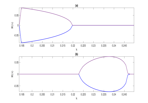
Figure 1: The real parts of the eigenvalues $(\lambda)$ corresponding to $P_{1}$ [Subplot (a)] and $P_{3}$ [Subplot (b)] are shown against the parameter $k$. The fixed parameter values are $\beta=8$, $\alpha=0.15$, and $n_{0}=10$. The bifurcations indicate that the system [Eq. (14)] can be stable with $\Re\lambda<0$ or unstable with $\Re\lambda>0$ around the fixed point $P_{1}$ or $P_{3}$ in a finite domain of $k$.

III.2 Lyapunov exponents, bifurcation diagram and phase-space portraits

Having predicted the stable and unstable regions of the dynamical system (14) in the domains of the wave number of modulation $k$ as in Sec. III, we proceed to establish the ranges of values of the parameters $k$, $\alpha$, and $\beta$ in which the periodic, quasiperiodic or chaotic states of plasma waves can exist. To this end, we first calculate the Lyapunov exponents $\Lambda_{i}$, $i=1,2,3,4$, for the dynamical system [Eq. (14)], to be written in the form $\dot{x}_{i}=f_{i}(X)$, with the initial condition: $X(0)=\left[x_{1}(0),~{}x_{2}(0),~{}x_{3}(0),~{}x_{4}(0)\right]$. We are interested in the evolution of attractors and depending on the initial condition, these attractors will be associated with different sets of exponents. The latter, however, describe the behaviors of $X(t)$ in the tangent space of the phase-space and are defined by the Jacobian matrix, given by,

$$J_{ij}(t)=\frac{df_{i}}{dx_{j}}\biggr{|}_{X(t)}.$$ (19)

The evolution of the tangent vectors can then be defined by the matrix $A$ via the following relation

$$\dot{A}=JA,$$ (20)

together with the initial condition $A_{ij}(0)=\delta_{ij}$. Here, $\delta_{ij}$ is the Kronecker delta and the matrix $A$ characterizes how a small change of separation distance between two trajectories in phase space develops from the starting point $X(0)$ to the final point $X(t)$. Nonetheless, the matrix $A$ is given by

$$A(t)=\begin{bmatrix}0&\beta_{0}\sin x_{4}&0&px_{2}\cos x_{4}\\ 0&0&1&0\\ -\alpha^{2}_{0}\cos x_{1}\cos x_{4}&-k^{2}&0&-\alpha_{0}^{2}\sin x_{1}\sin x_{4}\\ -\frac{1}{4}\beta_{0}x_{2}\sec^{2}(x_{1}/2)\cos x_{4}&-\frac{1}{2}\beta_{0}\tan(x_{1}/2)\cos x_{4}&0&-\frac{1}{2}x_{2}\tan(x_{1}/2)\sin x_{4}\end{bmatrix}.$$ (21)

The Lyapunov exponents $\Lambda_{i}$ are thus obtained as the eigenvalues of the following matrix.

$$\Lambda=\lim_{t\rightarrow\infty}\frac{1}{2t}\log\left[A(t)A^{T}(t)\right],$$ (22)

where $A^{T}$ denotes the transposed matrix of $A$. Given an initial condition $X(0)$, the separation distance between two trajectories in phase space or the change of particle’s orbit can be obtained by the Liouville’s formula: $\delta X(t)=\mathrm{tr}\left(J(t)\right)|A(t)|$, where $|A(t)|\equiv\mathrm{det}~{}A(t)$ and $\mathrm{det}~{}A(0)=1>0$. Thus, for the dynamical system (14), one obtains $\mathrm{det}~{}A(t)=\exp\left(\int_{0}^{t}\mathrm{tr}\left(J(t)\right)dt\right)=1>0$. It follows that at least one $\Lambda_{i}>0$, implying the existence of a chaotic state in a given time interval $[0,t]$.

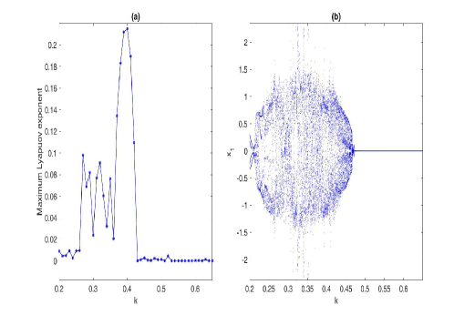
Figure 2: The maximum Lyapunov exponent [subplot (a)] and the bifurcation diagram [subplot (b)] are shown against the wave number $k$. The fixed parameter values are the same as in Fig. 1.

Before proceeding further to the analyses of Lyapunov exponent spectra and the bifurcation diagram together with the phase-space portraits, we recapitulate that the MI of Alfvén wave envelopes sets in for $0<k<k_{c}$. The growth rate of instability tends to become higher in the interval $0<k<(3/4)k_{c}$ and lower in $(3/4)k_{c}<k<k_{c}$ with a cut-off at $k=k_{c}$ at which the pitchfork bifurcation occurs. It follows that the nonlinear dynamics of wave-wave interactions is subsonic in the interval $(3/4)k_{c}<k<k_{c}$. However, as $k$ decreases from $(3/4)k_{c}$, many more unstable wave modes can be excited due to a selection of modes with $M=[k^{-1}]$ and the dynamics may no longer be subsonic. In this situation, a description of nonlinear interactions with three wave modes may be relatively correct. Thus, one may assume that one $(|m|=1)$ Alfvén wave mode is unstable (i.e., the Alfvén waves with $|m|>1$ are stable) and two driven ion-sound waves of plasma slow response (already excited by the unstable Alfvén mode) remain as they are. This leads to the autonomous system (14). We will investigate how the system behaves as the values of $k$ is successively increased from $(3/4)k_{c}$ to $k_{c}$ in the subsonic region and as $k$ reduces from $(3/4)k_{c}$ to a value so that the three-wave interaction model remains valid (since smaller the values of $k$ larger is the number of modes $M$).

In what follows, we calculate the maximum Lyapunov exponent $\lambda_{i}^{\text{max}}$ for Eq. (14) using the algorithm as stated above in a finite domain of $k$, i.e., $0<k<k_{c}<1$ and numerically solve Eq. (14) using the fourth order Runge-Kutta scheme with a time step $dt=10^{-3}$ to obtain the bifurcation diagram of a state variable $x_{1}$ and phase-space portraits with the same set of fixed parameter values $\beta=8$, $\alpha=0.15$, and $n_{0}=10$ as in Fig. 1. The results are displayed in Figs. 2 and 3. It is noted that, similar to subplot (b) of Fig. 1, two sub-intervals of $k$ exist, namely $0.2\lesssim k\lesssim k_{1}\approx 0.42$ and $k_{1}<k\lesssim 1$. In the former $\lambda_{i}^{\text{max}}>0$, while in the latter it is close to zero, implying that the system may exhibit chaotic states in $0.2\lesssim k\lesssim k_{1}$ and quasiperiodic and/or limit cycles in the other sub-interval [See subplot (a) of Fig. 2]. Physically, since lower (higher) values of $k~{}(<k_{1})$ correspond to a large (small) number of wave modes ($[k^{-1}]$) to participate in the nonlinear wave dynamics, the wave-wave interactions may result into chaos (limit cycles or steady states) by the influence of the nonlinearity associated with the Alfvén wave ponderomotive force (proportional to $\alpha$) and the nonlinear interactions between the fields (proportional to $\beta$). These features can also be verified from the bifurcation diagram of a state variable, e.g., $x_{1}$ with respect to the parameter $k$ [See subplot (b) of Fig. 2]. Here, it is seen that as the value of $k$ increases within the domain, a transition from chaotic (dense region) to a periodic or steady (straight line) state can occur. However, the values of $k$ smaller than $k=0.2$ may not be admissible as those correspond to a larger number of wave modes and their interactions can not be described by the low-dimensional system (14) but by the full system of equations (3) and (4). An investigation of the latter is, however, out of scope of the present work.

In order to further verify the dynamical features so predicted for ranges of values of $k$ and for illustration purpose, different phase-space portraits are also obtained by solving Eq. (14) numerically. From Fig. 3 it is evident that as the values of $k$ increase from smaller [subplots (a) and (b)] to larger ones [subplots (c) and (d)], the chaotic states of AWs transit into quasiperiodic [subplot (c)] and periodic [subplot (d)] states. These features are in agreement with the Lyapunov exponent and the bifurcation diagram shown in Fig. 2.

Thus, it is noted that the nonlinear interaction of a few wave modes of dispersive Alfvén waves and low-frequency plasma density perturbations can exhibit periodic, quasi-periodic and chaotic states in finite domains of the wave number of modulation due to the finite effects of the nonlinearities associated with the wave electric field driven ponderomotive force and the interactions of the electric field and the plasma density fluctuations. The existence of these states is established by the analyses of Lyapunov exponents, the bifurcation diagram and the phase-space portraits.

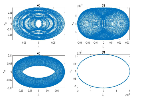
Figure 3: Different phase-space portraits, formed in the dynamical evolution of Eq. (14), are shown for different values of the wave number of modulation $k$: (a) $k=0.21$, (b) $k=0.42$, (c) $k=0.45$, and (d) $k=0.51$. Subplots (a) and (b) show the chaotic states while subplots (c) and (d) exhibit the quasi-periodic and periodic states respectively. The fixed parameter values are the same as in Fig. 1, i.e., $\beta=8$, $\alpha=0.15$ and $n_{0}=10$.

IV Characterization of chaos: measure of chaos complexity

In this section, we study the complexity of the dynamics of wave-wave interactions and thereby measure quantitatively the characteristics of chaotic behaviors of the state variables relating to plasma density or wave electric field perturbations. Although several formulas have been developed in the literature to characterize chaos, we focus mainly on the measures of embedding dimension estimation Wallot (2018), correlation dimension She et al. (2019), and the approximate entropy Pincus (1995, 1991); Delgado-Bonal and Marshak (2019).

IV.1 Estimation of Embedding parameters

Many well known and efficient techniques, e.g., Recurrence quantification technique for the analysis of nonlinear time series require the construction of phase-space profiles of the time series, since those techniques are applicable to the phase-space profiles but not to the time series themselves. The method of embedding dimension estimation is one such which also requires the reconstruction of successive phase spaces of chaotic processes with the effects of time delay.

Phase space reconstruction

Reconstruction of phase space has become useful to extract information of a chaotic time series in nonlinear dynamical systems. Let $X=\left[x(1),~{}x(2),...,x(n)\right]^{T}$ represent a uniformly sampled univariate time signal, i.e., an observed sequence of the chaotic state variable $x(t)$ (which may be any one of $x_{1},~{}x_{2},~{}x_{3}$, and $x_{4}$) with $t=1,2,...,n$. Then to reconstruct a phase space by embedding the dimension $m$, we construct a time series $Y(t)$ of length $m$ (i.e., $m$-dimensional points) from the original time series $X(t)$ by considering an appropriate time delay $\tau$ as

$$Y(t)=\left\{X(t),~{}X(t+\tau),...,X[t+(m-1)\tau]\right\}^{T},$$ (23)

where $t=1,2,...,n-(m-1)\tau$ and $\tau$ is a positive integer. Thus, the phase spaces of $M=n-(m-1)\tau$ state variables are reconstructed. Generalizing this result, one can reconstruct the phase spaces for multivariate time signals. So, in order to perform the phase-space reconstruction, one must know the two embedding parameters, namely the time delay parameter $\tau$, which is the lag at which the time series has to be plotted against itself, and the embedding dimension parameter $m$, where $m-1$ is the number of times that the time series has to be plotted against itself using the delay $\tau$. Having known these two parameters, one can then reconstruct an approximate phase-space of the original one from a given time series. In the following two subsections, we estimate these two parameters by the methods of computing the two functions, namely the Average mutual information (AMI) and the False nearest neighbors (FNN) Wallot (2018) in which the first local minima (or the points of cut-off) of these functions can be estimated as the time delay and the embedding dimension respectively.

Average mutual information (AMI): Estimation of time delay

In AMI, the mutual information is computed between the original time series of a state variable $X(t)$ and a time shifted version of the same time series, i.e., $X(t+\tau)$. This average or auto mutual information can be considered as a nonlinear generalization of the auto correlation function, given by,

$$I\left[X(t),X(t+\tau)\right]=\sum_{i,j}p_{ij}(\tau)\log\left(\frac{p_{ij}(\tau)}{p_{i}p_{j}}\right),$$ (24)

where $p_{i}$ is the probability that $X(t)$ is in the $i$th rectangle of the histogram to be constructed from the data points of $X(t)$ and $p_{ij}$ is the probability that $X(t)$ is in the $i$th rectangle and $X(t+\tau)$ in the $j$th rectangle.

False nearest neighbors (FNN): Estimation of embedding dimension

Typically, the embedding dimension $m$ for phase-space reconstruction is estimated by inspecting the change in distance between two nearest points in phase-space as one gradually embeds the original time series $X(t)$ into higher dimensional ones $Y(t)$. The use of FNN, as prescribed by Kennel et al. Kennel et al. (1992), is based on the following logic: Initially, we have the one-dimensional time series $X(t),~{}t=1,2,...,n$ and the distance between two of its neighboring points are noted. Then we embed $X(t)$ into two dimensions $Y(t)=\left\{X(t),~{}X(t+\tau)\right\}$ with some time delay $\tau$ and examine whether there is any considerable change in the distance between any two neighboring data points of $Y(t)$. If so, these data points are said to be false neighbors, and the data points need to be embedded further. Otherwise, if the change is not significant, the data points are called true neighbors and the embedding retains the shape of the phase-space attractor, implying that the present embedding dimension is sufficient. This process of successively increasing the embedding dimension $m$ can be continued until the number of FNN reduces to zero, or the subsequent embedding does not alter the number of FNNs, or the number of FNNs starts to increase again. A working algorithm for calculating FNN for our system can be stated below.

• Identify the nearest point in the Euclidean sense to a given point of the time-delay coordinates. That is, for a given time series $Y(t)=\left\{X(t),~{}X(t+\tau),...,X[t+(m-1)\tau]\right\}^{T}$, find a point $Y_{i}$ in the data set such that the distance $m=\|Y_{i}-Y_{j}\|_{2}$ is minimized, where $Y_{i}$ and $Y_{j}$ denote the nearest neighboring data points of $Y(t)$.

• Determine whether the following expression is true or false:

  $$\frac{|X_{i}-X_{j}|}{\|Y_{i}-Y_{j}\|}\leq\mathrm{Distance~{}threshold~{}(R)},$$ (25)

  where $X_{i}$ and $X_{j}$ denote the nearest neighboring data points of $X(t)$. If the condition in Eq. (25) is satisfied, then the neighbors are true nearest neighbors, otherwise they are false nearest neighbors.

• Perform the step 2 for all points $i$ in the data set and calculate the percentage of points in the data set that have false nearest neighbors.

• Increase embedding the dimension until the percentage of false nearest neighbors drops to zero or an admissible small number.

Following Ref. Wallot (2018) and using MATLAB, we estimate the embedding parameters, namely the time lag $\tau$ and the embedding dimension $m$ for the four-dimensional time series $(x_{1},~{}x_{2},~{}x_{3},~{}x_{4})$ formed by all the four variables of the system (14). The results are shown in Fig. 4. From subplot (a), we find that all the auto mutual information (AMI) curves, obtained for different time series, cut the threshold line at different values of $\tau$. It is seen that for these curves, the AMI first drops below the threshold value $(1/e)$ after the time lags $\tau=4.25,~{}5.75,~{}13.1$, and $19.66$, and we have considered the maximum time delay as $\tau=25$. Thus, a mean value of $\tau$ for each dimension can be obtained as $\tau=(4.25+5.75+13.1+19.66)/4=10.7$ for which we obtain an estimate for $\tau$ as $\tau=11$. On the other hand, subplot (b) displays the FNN function against the embedding dimension $m$. It is clear that the available four-dimensional time series is sufficient and no further time-delayed embedding of dimension is required.

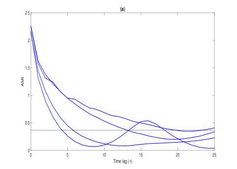
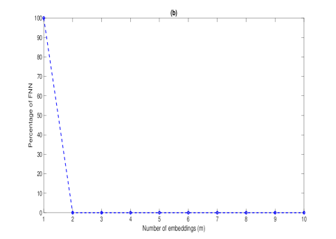
Figure 4: The graphical output(s) of the average mutual information (AMI) function [Subplot (a)] and percentage of false nearest neighborhoods (FNN) function [Subplot (b)] are shown against the time lag $\tau$ and the embedding dimension $m$ respectively for the four-dimensional time series taken from Eq. (14). In the upper panel, the default threshold value $(1/e)$ is shown by the horizontalline. The dashed line in the lower panel shows an immediate drop-off of the percentage of false-nearest neighbors to zero, indicating that no additional embedding is necessary for the time series.

Next, having estimated the time delay $\tau=11$ and the embedding dimension $m>2$ a reconstruction of phase space is shown in Fig. 5 for all the variables $x_{1}$, $x_{2}$, $x_{3}$, and $x_{4}$ of Eq. (14). Here, the time series for the variables are plotted against each other with the time lag $\tau=11$. It is seen that the resulting phase space with the time lag is approximately the same as the original one.

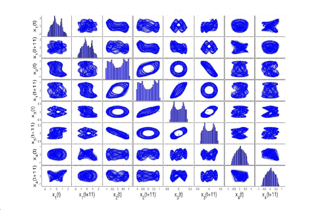
Figure 5: Reconstruction of phase-space with the time lag, $\tau=11$ and embedding dimension, $m=4$ from the chaotic time series of Eq. (14).

IV.2 Correlation dimension estimation

One of the most important measures of complexity of chaotic attractors is the correlation (or fractal) dimension. It has been shown by many researchers that the correlation dimension is more pertinent to experimental data than the capacity dimension as it simply calibrates the geometrical structure of an attractor and is insufficient for higher dimensional systems. Moreover, the correlation dimension is a (or close to the) lower bound on the Hausdorff fractal dimension, which is infinite for noise; positive and finite for a deterministic system; integer for integrable systems, and non-integer for a chaotic deterministic system. The derivation of the correlation dimension also requires the reconstruction of vectors from the time series $X(t)$, i.e.,

$$\begin{split}Y_{1}(t)&=\left\{X(t),~{}X(t+\tau),...,X[t+(m-1)\tau]\right\}^{T},\\ Y_{2}(t)&=\left\{X(t+p),...,X[t+p+(m-1)\tau]\right\}^{T},\\ &\vdots\\ Y_{M}(t)&=\left\{X(t+Mp),...,X[t+Mp+(m-1)\tau]\right\}^{T},\end{split}$$ (26)

where $p$ (a positive integer) and $\tau$, respectively, stand for the inter-vector and intra-vector spacing.

After the reconstruction of phase space of a chaotic signal $X(t)$ with $M$ vectors and computing the correlated vector pairs, its proportion in all possible pairs in $M^{2}$ is the correlation integral $C(l)$, given by,

$$C(l)=\lim_{M\rightarrow\infty}\left[\frac{2}{M^{2}}\sum_{i=1}^{M-k}\sum_{j=i+k}^{M}\Theta\left(l-|X(i)-X(j)|\right)\right],$$ (27)

where $X(i)$ and $X(j)$ are the position vectors of pints on an attractor, $l$ is the distance under inspection, $k$ is the summation offset used to prevent proximate vectors being counted, and $\Theta(x)$ is the Heaviside step function, defined by,

$$\Theta(x)=\left\{\begin{array}[]{cc}0,&x\leq 0\\ 1,&x>0.\end{array}\right.$$ (28)

The correlation dimension $d$ is then calculated from the correlation integral as

$$d=\lim_{l\rightarrow 0}\frac{\log{C(l)}}{\log{l}}.$$ (29)

Next, using Eq. (29) we plot a graph of $\log{C(l)}$ vs $\log{l}$ for the time series $X(t)$ of the dynamical system (14) with a fixed embedding dimension $m=4$ and time delay $\tau=11$. The system is turned to be higher dimensional by the method described above. As a comparison we have also obtained graphs of the correlation integrals for the Hénon map with the embedding dimension $m=2$ and the Lorenz system with $m=3$. The results are displayed in Fig. 6. The fixed parameter values considered here are the same as Fig. 1, i.e., $\alpha=0.15$, $\beta=8$, and $n_{0}=10$. The slopes of the straight-line portions (obtained using the least-square curve fitting) of the graphs represent the correlation dimensions. For the present system [Eq. (14)] the results as in subplot (a) appear similar to those for the Hénon map [subplot (b)] and the Lorenz system [subplot (c)]. However, the correlation dimension obtained for our system is $d=1.0776$, while for the Hénon map and the Lorenz system are $d=1.25$ and $d=2.06$ respectively. It follows that the system (14) is chaotic and possesses a strange attractor characterized by $d=1.0776$.

In Fig. 7, we plot $\log{C(l)}$ vs $\log{l}$ for increasing values of the embedding dimension, namely $m=8,~{}12,~{}16$, and $20$. The time series is taken to be consisted of $10000$ points separated by the time lag $\tau=11$. One can then obtain the correlation dimensions as $d=1.0777,~{}1.0781,~{}1.0788$ respectively. Thus, a series of straight lines indeed exist with slopes $d\approx 1.07\pm 0.01$ and $\log{C(l)/\log{l}}$ is nearly a constant value for large $m$.

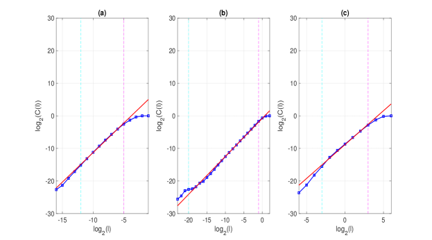
Figure 6: Plots of the log-correlation integral $[\log{C(l)}]$ vs the log-correlation dimension $(\log{l})$ are shown for (a) the present model [Eq. 14], (b) for the Hénon map, (c) for the Lorenz system. The correlation dimensions obtained for the subplots (a), (b), and (c) are $d=1.0776$, $1.25$, and $2.06$ respectively.

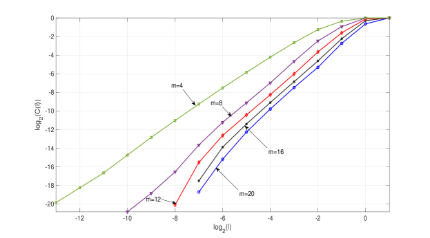
Figure 7: Plot of the log-correlation integral $[\log{C(l)}]$ vs the log-correlation dimension $(\log{l})$ with different embedding dimensions: $m=4,~{}8,~{}12,~{}16,~{}20$ and $10,000$ observations is shown for Eq.(14). The parameter values are the same as Fig. 1, i.e., $\beta=8$, $\alpha=0.15$, and $n_{0}=10$ together with $k=0.35$.

Model	Control parameter	Correlation dimension(d) for different values of $k$ and $m$					Hausdorff fractal dimension (D)
		d (m=4)	d (m=8)	d (m=12)	d (m=16)	d (m=20)
Our Dynamical Model	k=0.13	1.0776	1.0777	1.0781	1.0788	1.0811	$1.0646\pm 0.013997$
	k=0.23	1.0453	1.0465	1.0473	1.0483	1.0535
	k=0.28	1.0718	1.0724	1.0733	1.0740	1.0747
	k=0.33	1.0720	1.0705	1.0694	1.0686	1.0767
	k=0.38	1.0721	1.0706	1.0696	1.0684	1.0677
	k=0.5	1.00069	1.00068	1.00065	1.00063	1.00061	$1.00047\pm 0.00068262$
Henon map	a=1.4	1.2541	1.4850	1.6445	2.0881	3.1845	$1.260303\pm 0.003$
	a=1.3	1.2510	1.4516	1.6565	2.1834	2.6294
	a=1.25	1.2506	1.4615	1.6756	2.1225	2.6252
	a=1.2	1.2501	1.4589	1.6946	2.1045	2.6052
	a=1.15	1.2408	1.4568	1.6725	2.0768	2.6466
	a=1.1	1.2659	1.4588	1.6767	2.04794	2.6246
Lorenz system	$\rho=28$	2.0866	2.7763	3.0121	3.1246	3.3623	2.06 $\mathrm{\pm}$ 0.01
	$\rho=26$	2.1670	2.3767	2.5679	2.6844	2.8563
	$\rho=24$	1.8288	2.0223	1.9516	2.1235	2.4874
	$\rho=22$	2.1999	2.0413	1.9608	2.0915	2.4599
	$\rho=20$	0.01047	0.0779	0.0478	0.0148	0.0048	$2.0002\pm 0.00048023$
	$\rho=15$	0.0079	0.0076	0.0075	0.0072	0.0071

Table 1: Estimations for the correlation dimension $(d)$ and the Hausdroff fractal dimension $(D)$ are shown for the present model, the Hénon map and the Lorenz system with different values of $m$ and the control parameter $k$ and with a fixed $10000$ observations.

In what follows, we calculate the correlation dimension $(d)$ and the Hausdroff fractal dimension $(D)$ [For details, see, e.g., Ref. Mori (1980)] of a time series of Eq. (14) with different values of the control parameter $k$ and the embedding dimension $m$. The results are compared with those of the Hénon map and the Lorenz system. A summary of the results is presented in Table 1. It is noted that even with an increasing value of the embedding dimension and a change of value of the parameter $k$, the correlation dimension $d$ converges to a constant value. The bounds for the Hausdroff dimension of the chaotic time series are also calculated. It is seen that the correlation dimension lies within the bounds of the Hausdroff dimension.

IV.3 Approximate entropy (ApEn)

Although a number of techniques are used to measure the complexity of a chaotic system, not all are applicable to limited, noisy and stochastically derived time series. For example, the Kolmogorov-Sinai (KS) entropy works well for real dynamical systems but not for systems with noise Delgado-Bonal and Marshak (2019). Also, the finite correlation dimension value discussed before can not guarantee that the system under consideration is deterministic. Furthermore, the Pincus technique fails for systems dealing with stochatic components. In this situation, the Approximate Entropy (ApEn) is more applicable to measure the system’s complexity compared to others in which the statistical precision is compromised Delgado-Bonal and Marshak (2019). The ApEn estimates uniformly sampled time-domain signals through phase space reconstruction and then measures the amount of regularity and unpredictability of fluctuations in a time series.

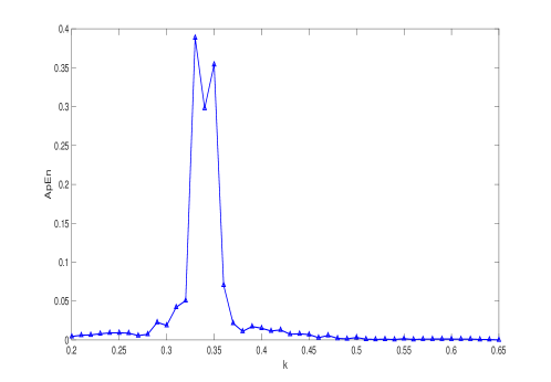
Figure 8: Approximate entropy (ApEn) is shown against the parameter $k$ for Eq. 14 with $m=4$, $l=0.1$, and $N=5000$. The other parameter values are the same as Fig. 1, i.e., $\beta=8$, $\alpha=0.15$, and $n_{0}=10$.

For an $N$ given data points together with the embedding dimension $m$ and the correlation integral $C(l)$, the ApEn is defined by

$${\rm{ApEn}}(m,l,N)=\Phi^{m}(l)-\Phi^{m+1}(l),$$ (30)

where

$$\Phi^{m}(l)=\frac{\sum_{i=1}^{N-m+1}\log C^{m}_{i}(l)}{N-m+1}.$$ (31)

We have calculated the ApEn against the controlling parameter $k$ (The other parameter values are the same as Fig. 1, i.e., $\beta=8$, $\alpha=0.15$, and $n_{0}=10$) and for a given set of values, namely $m=4$ and $l=0.1$ together with $5000$ data points. The results are shown graphically in Fig. 8. It is noted that while the ApEn assumes high values in the subdomain $0.275\lesssim k\lesssim 0.4$ in which the Lyapunov exponent is found to be positive (cf. Fig. 2) its values are low in rest of the domain where the Lyapunov exponents are close to zero. Thus, low values of ApEn predict that the system is steady, tedious and predictive, while high values imply the independence between the data, a low number of repeated patterns, and randomness.

V Conclusion

We have investigated the dynamical properties of dispersive Alvén waves coupled to plasma slow response of electron and ion density perturbations in a uniform magnetoplasma. By restricting the nonlinear wave-wave interactions to a few numbers of active wave modes, a low-dimensional autonomous system is constructed which is shown to exhibit periodic, quasiperiodic and chaotic states by means of the analyses of Lyapunov exponent spectra, bifurcation diagram, and phase-space portraits. The low-dimensional autonomous system can be a good approximation for the nonlinear interaction of Alfvén waves coupled to driven ion-sound waves associated with plasma slow response of density fluctuations in the stable or plane wave region $(3/4)k_{c}<k<k_{c}<1$. In the latter, the modulational instability growth rate of Alvén wave envelopes is low. The model can be relatively accurate in the region $0.2\lesssim k<(3/4)k_{c}$ (in which the condition for the subsonic region is relaxed and the instability growth rate is relatively high) where the low-dimensional model exhibits chaos for given values of the the pump electric field $E_{0}$ as well as the parameters $\alpha$, $\beta$, and $n_{0}$, associated with the relative speeds of the Alvén waves compared to the speed of light in vacuum and the ion-sound speed, and the conserved plasmon number respectively. However, for values of $k<0.2$, the low-dimensional model will no longer be valid for the description of wave-wave interactions as smaller values of $k$ correspond to the excitation of a large number of unstable modes.

The complexity of chaotic phase-space structures of chaotic time series is also measured quantitatively by means of the correlation dimension and the approximate entropy through the reconstruction of phase spaces and estimation of embedding parameters, namely the time lag and the embedding dimension. It is found that even with an increasing value of the embedding dimension and with a slightly different set of values of the parameters $\alpha$, $\beta$, $n_{0}$, and $k$, the correlation dimension converges to a constant value. The bounds for the Hausdroff fractal dimension of the chaotic time series are also calculated to show that the correlation dimension lies in between the bounds. Furthermore, the results are shown to be a good qualitative agreement with those for the Hénon map and the Lorenz system.

To conclude, the existence of chaos and its complexity in the low-dimensional interaction model can be a good signature for the emergence of spatiotemporal chaos in the full system of equations (1) and (2) where the participation of many more wave modes (more than three) in the nonlinear interactions can be possible. Such chaotic aspects of Alvén waves can be relevant for the onset of turbulence due to flow of energy from lower to higher harmonic modes (i.e., with large to small spatial length scales) in the Earth’s ionosphere and magnetosphere.

Data Availability

The data that support the findings of this study are available from the corresponding author upon reasonable request.

Appendix A Derivation of the dispersion relation [Eq. (6)]

Here, we give some relevant details for the derivation of the dispersion relation (6) for the modulated DAW envelope. We rewrite Eqs. (3) and (4) as

$$\frac{\partial^{2}n}{\partial t^{2}}-\frac{\partial^{2}n}{\partial z^{2}}=-\alpha^{2}\frac{\partial^{2}}{\partial z^{2}}|E|^{2},$$ (32)

$$\frac{\partial E}{\partial t}+\beta\frac{\partial E}{\partial z}-\frac{\beta}{2}\frac{\partial}{\partial z}(nE)+i\gamma\frac{\partial^{2}E}{\partial z^{2}}=0,$$ (33)

We assume the wave electric field envelope to be of the form $E=\tilde{E}e^{i\theta(z,t)}$ and the density perturbation as $n=\tilde{n}(z,t)$. Then Eqs. (32) and (33) reduce to

$$\frac{\partial^{2}\tilde{n}}{\partial t^{2}}-\frac{\partial^{2}\tilde{n}}{\partial z^{2}}=-\alpha^{2}\frac{\partial^{2}}{\partial z^{2}}|\tilde{E}|^{2},$$ (34)

$$\begin{split}\frac{\partial\tilde{E}}{\partial t}+&i\tilde{E}\frac{\partial\theta}{\partial t}+\beta\left(\frac{\partial\tilde{E}}{\partial z}+i\tilde{E}\frac{\partial\theta}{\partial t}\right)-\frac{\beta}{2}\left[\frac{\partial}{\partial z}(\tilde{n}\tilde{E})+i\tilde{E}\tilde{n}\frac{\partial\theta}{\partial z}\right]\\ &+i\gamma\left[\frac{\partial^{2}\tilde{E}}{\partial z^{2}}+2i\frac{\partial\tilde{E}}{\partial z}\frac{\partial\theta}{\partial z}+i\tilde{E}\frac{\partial^{2}\theta}{\partial z^{2}}-\tilde{E}\left(\frac{\partial\theta}{\partial z}\right)^{2}\right]=0,\end{split}$$ (35)

Separating the real and imaginary parts of Eq. (35), we get

$$\frac{\partial\tilde{E}}{\partial t}+\beta\frac{\partial\tilde{E}}{\partial z}-\frac{\beta}{2}\frac{\partial}{\partial z}(\tilde{n}\tilde{E})-\gamma\left(\tilde{E}\frac{\partial^{2}\theta}{\partial z^{2}}+2\frac{\partial\tilde{E}}{\partial z}\frac{\partial\theta}{\partial z}\right)=0,$$ (36)

$$\tilde{E}\frac{\partial\theta}{\partial t}+\beta\tilde{E}\frac{\partial\theta}{\partial z}-\frac{\beta}{2}\tilde{E}\tilde{n}\frac{\partial\theta}{\partial z}+\gamma\left[\frac{\partial^{2}\tilde{E}}{\partial z^{2}}-\tilde{E}\left(\frac{\partial\theta}{\partial z}\right)^{2}\right]=0.$$ (37)

Looking for the modulation of the Alfvén wave envelope, we make the following ansatz:

$$\begin{split}\tilde{E}(z,t)=E_{0}+E_{1}\cos{(kz-\omega t)}+E_{2}\sin{(kz-\omega t)},\\ \tilde{n}(z,t)=n_{1}\cos{(kz-\omega t)}+n_{2}\sin{(kz-\omega t)},\\ \theta(z,t)=\theta_{0}+\theta_{1}\cos{(kz-\omega t)}+\theta_{2}\sin{(kz-\omega t)},\end{split}$$ (38)

where $E_{0},~{}E_{1},~{}E_{2},~{}n_{1},~{}n_{2},~{}\theta_{0},~{}\theta_{1}$, and $\theta_{2}$ are real constants.

Substituting Eq. (38) into Eqs. (34), (36), and (37) and linearizing (retaining only the first harmonic terms), we get

$$\begin{split}&\left[(\omega^{2}-k^{2})n_{1}+2\alpha^{2}k^{2}E_{0}E_{1}\right]\cos{(kz-\omega t)}\\ &+\left[(\omega^{2}-k^{2})n_{2}+2\alpha^{2}k^{2}E_{0}E_{2}\right]\sin{(kz-\omega t)}=0,\end{split}$$ (39)

$$\begin{split}&[(\omega-\beta k)E_{2}+\frac{\beta}{2}E_{0}kn_{2}-\gamma E_{0}k^{2}\theta_{1}]\cos{(kz-\omega t)}\\ &-[(\omega-\beta k)E_{1}+\frac{\beta}{2}E_{0}kn_{1}+\gamma E_{0}k^{2}\theta_{2}]\sin{(kz-\omega t)}=0,\end{split}$$ (40)

$$\begin{split}&[(\omega-\beta k)E_{0}\theta_{2}+\gamma k^{2}E_{1}]\cos{(kz-\omega t)}\\ &-[(\omega-\beta k)E_{0}\theta_{1}-\gamma k^{2}E_{2}]\sin{(kz-\omega t)}=0.\end{split}$$ (41)

Equating the coefficients of different harmonics proportional to $\cos{(kz-\omega t)}$ and $\sin{(kz-\omega t)}$ to zero, we successively obtain

$$(\omega^{2}-k^{2})n_{1}+2\alpha^{2}k^{2}E_{0}E_{1}=0,$$ (42)

$$(\omega^{2}-k^{2})n_{2}+2\alpha^{2}k^{2}E_{0}E_{2}=0,$$ (43)

$$(\omega-\beta k)E_{2}+\frac{\beta}{2}E_{0}kn_{2}-\gamma E_{0}k^{2}\theta_{1}=0,$$ (44)

$$(\omega-\beta k)E_{1}+\frac{\beta}{2}E_{0}kn_{1}+\gamma E_{0}k^{2}\theta_{2}=0,$$ (45)

$$(\omega-\beta k)E_{0}\theta_{2}+\gamma k^{2}E_{1}=0,$$ (46)

$$(\omega-\beta k)E_{0}\theta_{1}-\gamma k^{2}E_{2}=0.$$ (47)

Next, eliminating $\theta_{1}$ and $\theta_{2}$ from Eqs. (44)-(47), we get

$$[(\omega-\beta k)^{2}-\gamma^{2}k^{4}]E_{1}+\frac{\beta}{2}(\omega-\beta k)E_{0}kn_{1}=0,$$ (48)

$$[(\omega-\beta k)^{2}-\gamma^{2}k^{4}]E_{2}+\frac{\beta}{2}(\omega-\beta k)E_{0}kn_{2}=0.$$ (49)

Furthermore, eliminating either $n_{1}$ from Eqs. (42) and (48) or eliminating $n_{2}$ from Eqs. (43) and (49), and noting that $E_{1},~{}E_{2}\neq 0$, we obtain

$$(\omega^{2}-k^{2})[(\omega-\beta k)^{2}-\gamma^{2}k^{4}]-\alpha^{2}\beta k^{3}|E_{0}|^{2}(\omega-\beta k)=0.$$ (50)

From Eq. (50), it is noted that while the first term represents a coupling between the Alfvén wave and the ion-acoustic density perturbation, the second term proportional to $|E_{0}|^{2}$ appears due to the Alfvén wave driven ponderomotive force. In absence of the latter, we have the usual acoustic mode $\omega=k$ and the following Alfvén wave dispersion equation.

$$\omega-\beta k=-\gamma k^{2},$$ (51)

where the negative sign (on the right-hand side) is considered in order to satisfy Eq. (33) for the wave eigenmode. So, treating the term proportional to $|E_{0}|^{2}$ as the correction term in Eq. (50) and replacing $(\omega-\beta k)$ by $-\gamma k^{2}$ therein, we obtain the following dispersion law for the modulated Alfvén wave envelope.

$$(\omega^{2}-k^{2})[(\omega-\beta k)^{2}-\gamma^{2}k^{4}]+\alpha^{2}\beta\gamma k^{5}|E_{0}|^{2}=0.$$ (52)

Next, to obtain the growth rate of instability, we assume $\omega\approx\beta k+i\Gamma$ with $\beta k\gg\Gamma,~{}\gamma k^{2}$, Thus, Eq. (52) gives

$$[(\beta^{2}-1)k^{2}-\Gamma^{2}+2i\beta k\Gamma](\Gamma^{2}+\gamma^{2}k^{4})-\alpha^{2}\beta\gamma k^{5}|E_{0}|^{2}=0.$$ (53)

Since the term proportional to $i$ in Eq. (53) does not give any admissible result, we equate the real part to zero. Thus, we obtain

$$[(\beta^{2}-1)k^{2}-\Gamma^{2}](\Gamma^{2}+\gamma^{2}k^{4})-\alpha^{2}\beta\gamma k^{5}|E_{0}|^{2}=0.$$ (54)

Using $\beta k\gg\gamma k^{2}$ and neglecting the terms containing higher orders (than the second order) of $\Gamma$, we obtain from Eq. (54) the following expression for the growth rate of instability.

$$\Gamma^{2}=\gamma k^{3}\left(\frac{\beta\alpha^{2}|E_{0}|^{2}}{\beta^{2}-1}-\gamma k\right).$$ (55)

Appendix B Derivation of the low-dimensional model [Eqs. (11)-(13)]

We recast Eqs. (3) and (4) as

$$\frac{\partial^{2}n}{\partial t^{2}}-\frac{\partial^{2}n}{\partial z^{2}}=-\alpha^{2}\frac{\partial^{2}}{\partial z^{2}}|E|^{2},$$ (56)

$$\frac{\partial E}{\partial t}+\beta\frac{\partial E}{\partial z}-\frac{\beta}{2}\frac{\partial}{\partial z}(nE)+i\gamma\frac{\partial^{2}E}{\partial z^{2}}=0.$$ (57)

Next, we consider an one dimensional spectrum for each of the the wave electric field $E$ and the plasma density perturbation $n$, which describe the general solution of Eqs. (56) and (57) as a superposition of a set of normal modes, i.e.,

$$E(z,t)=E_{0}(t)+E_{-1}(t).e^{-ikz}+E_{1}(t).e^{ikz},$$ (58)

$$n(z,t)=n_{0}(t)+n_{1}(t).e^{ikz}+n_{1}^{*}(t).e^{-ikz},$$ (59)

where $E_{-1}(0)=E_{1}(0)$.

Substituting these expressions for $E$ and $n$ into (57) and following the same approach as in Refs. Banerjee et al. (2010); Misra et al. (2010), we obtain

$$i\dot{E}_{0}=0,$$ (60)

$$\dot{E}_{1}+ik\beta E_{1}-ik^{2}\gamma E_{1}=i\frac{k\beta}{2}(n_{0}E_{1}+n_{1}E_{0}),$$ (61)

$$\dot{E}_{-1}-ik\beta E_{-1}-ik^{2}\gamma E_{-1}=-i\frac{k\beta}{2}(n_{0}E_{-1}+n_{1}^{*}E_{0}),$$ (62)

where the dot denotes the differentiation with respect to $t$ and the asterisk denotes the complex conjugate. Multiplying Eq (60) by $E_{0}^{*}$ we obtain

$$i|\dot{E_{0}}|^{2}=0.$$ (63)

Also, multiplying Eqs. (61) and (61) successively by $E_{1}^{*}$ and $E_{-1}^{*}$ and subtracting the complex conjugate of the resulting equations from themselves, we get

$$i|\dot{E_{-1}}|^{2}=\frac{k\beta}{2}(n_{1}^{*}E_{0}E_{-1}^{*}-n_{1}E_{0}E_{-1}),$$ (64)

$$i|\dot{E_{1}}|^{2}=\frac{k\beta}{2}(n_{1}^{*}E_{0}E_{1}-n_{1}E_{0}E_{1}^{*}),$$ (65)

where $\dot{|E|}^{2}=\frac{d}{dt}|E|^{2}$. Equations (63)-(65) can be added to yield

$$|E_{-1}|^{2}+|E_{1}|^{2}+|E_{0}|^{2}=N.$$ (66)

Next, we assume $n_{1}=n_{1}^{*},~{}n_{0}=N$, the plasmon number, and introduce the new variables $\rho_{0},~{}\rho_{1},~{}\theta_{0}$, and $\theta_{1}$ according to $E_{0}=\rho_{0}e^{i\theta_{0}},E_{-1}=E_{0}=\rho_{1}e^{i\theta_{1}},\rho_{0}=\sqrt{n_{0}}\sin{w},\rho_{1}=\sqrt{n_{0}}\cos{w},\psi=2w$.

Substituting the expressions (58) and (59) into Eq. (56) and using the new variables as defined above, we get

$$\ddot{n_{1}}-k^{2}n_{1}=\alpha^{2}k^{2}n_{0}\sin{\psi}\cos{\phi}.$$ (67)

Also, using the newly defined varibles, from Eqs. (61) and (62) we obtain

$$\dot{\psi}=\beta kn_{1}\sin{\phi},$$ (68)

$$\dot{\phi}=k(\beta-\gamma k)-\frac{1}{2}\beta kn_{1}\tan{\frac{\psi}{2}}\cos\phi.$$ (69)

where $\phi=\theta_{0}-\theta_{1}$. Equations (67)-(69) constitute the required low-dimensional model.

Appendix C Equilibrium points of Eq. (14)

To find the equilibrium points of Eq. (14), we equate the right-hand side expression of each of Eq. (14) to zero. Thus, we successively obtain

$$\begin{split}&\beta_{0}x_{2}\sin{x_{4}}=0,\\ &x_{3}=0,\\ &-k^{2}x_{2}+\alpha_{0}^{2}\sin{x_{1}}\cos{x_{4}}=0,\\ &\gamma_{0}-\frac{1}{2}\beta_{0}x_{2}\tan\frac{x_{1}}{2}\cos{x_{4}}=0,\end{split}$$ (70)

where $\beta_{0}=\beta k$, $\alpha_{0}=\alpha k\sqrt{n_{0}}$ and $\gamma_{0}=k(\beta-\gamma k)$. Since $(0,0,0,0)$ is not an equilibrium point (as explained in Sec. III.1), we have $x_{2}\neq 0$. So, the first equation of Eq. (70) gives $\sin{x_{4}}=0$, i.e., $x_{4}=n\pi$. Using this value of $x_{4}$ in the third equation of Eq. (70), one obtains $x_{2}=(-1)^{n}(\alpha_{0}^{2}/k^{2})\sin{x_{1}}$, since $\cos(n\pi)=(-1)^{n}$, $n$ being zero or an integer. Having obtained the values of $x_{2}$ and $x_{4}$, and using those in the fourth equation of Eq. (70), we get $x_{1}=4n\pi\pm 2\sin^{-1}\left(\sqrt{{\gamma_{0}k^{2}}/{\alpha_{0}^{2}\beta_{0}}}\right)$. Thus, the equilibrium points of Eq. (14) can be obtained as $(x_{10},x_{20},0,n\pi)$, where $x_{10}=4n\pi\pm 2\sin^{-1}\left(\sqrt{{\gamma_{0}k^{2}}/{\alpha_{0}^{2}\beta_{0}}}\right)$ and $x_{20}=\pm(-1)^{n}\left({2k}/{\beta_{0}}\right)\sqrt{\left(\beta-\gamma k\right)\left(\alpha^{2}n_{0}\beta-\beta+\gamma k\right)}$, where $n$is zero or an integer.

References

- Jana et al. (2017) S. Jana, S. Ghosh, and N. Chakrabarti, Physics of Plasmas 24, 102307 (2017), https://doi.org/10.1063/1.4994118 .
- Alfvén (1942) H. Alfvén, Nature 150, 405 (1942).
- Lundquist (1949) S. Lundquist, Physical Review 76, 1805 (1949).
- Vogt (2002) J. Vogt, Surveys in Geophysics 23, 335 (2002).
- Tsurutani and Ho (1999) B. T. Tsurutani and C. M. Ho, Reviews of Geophysics 37, 517 (1999).
- Nakariakov et al. (1999) V. Nakariakov, L. Ofman, E. Deluca, B. Roberts, and J. Davila, Science 285, 862 (1999).
- Bloxham et al. (2002) J. Bloxham, S. Zatman, and M. Dumberry, Nature 420, 65 (2002).
- Shukla et al. (2004) P. K. Shukla, L. Stenflo, R. Bingham, and B. Eliasson, Plasma Physics and Controlled Fusion 46, B349 (2004).
- Gekelman (1999) W. Gekelman, Journal of Geophysical Research: Space Physics 104, 14417 (1999).
- Shi et al. (2017) M. Shi, H. Li, C. Xiao, and X. Wang, The Astrophysical Journal 842, 63 (2017).
- Jain et al. (1986) K. M. Jain, M. Bose, S. Guha, and D. P. Tewari, Journal of Plasma Physics 36, 189–193 (1986).
- Wang et al. (2020) F. Wang, , J. Han, and W. Duan, Plasma Science and Technology 23, 015002 (2020).
- Mjolhus and Wyller (1986) E. Mjolhus and J. Wyller, Physica Scripta 33, 442 (1986).
- Roberts et al. (2016) O. W. Roberts, X. Li, O. Alexandrova, and B. Li, Journal of Geophysical Research: Space Physics 121, 3870 (2016), https://agupubs.onlinelibrary.wiley.com/doi/pdf/10.1002/2015JA022248 .
- Chmyrev et al. (1988) V. M. Chmyrev, S. V. Bilichenko, O. A. Pokhotelov, V. A. Marchenko, V. I. Lazarev, A. V. Streltsov, and L. Stenflo, Physica Scripta 38, 841 (1988).
- Shukla and Stenflo (1995) P. K. Shukla and L. Stenflo, Physica Scripta T60, 32 (1995).
- Misra and Shukla (2009) A. P. Misra and P. K. Shukla, Phys. Rev. E 79, 056401 (2009).
- Banerjee et al. (2010) S. Banerjee, A. P. Misra, P. K. Shukla, and L. Rondoni, Phys. Rev. E 81, 046405 (2010).
- Zakharov et al. (1975) V. E. Zakharov, A. F. Mastryukov, and V. S. Synakh, Fizika Plazmy 1, 614 (1975).
- Misra and Banerjee (2011) A. P. Misra and S. Banerjee, Phys. Rev. E 83, 037401 (2011).
- Shukla et al. (1986) P. K. Shukla, M. Y. Yu, and L. Stenflo, Physica Scripta 34, 169 (1986).
- Misra et al. (2010) A. P. Misra, S. Banerjee, F. Haas, P. K. Shukla, and L. P. G. Assis, Physics of Plasmas 17, 032307 (2010), https://doi.org/10.1063/1.3356059 .
- Kawata and Inoue (1978) T. Kawata and H. Inoue, Journal of the Physical Society of Japan 44, 1968 (1978), https://doi.org/10.1143/JPSJ.44.1968 .
- Kaup and Newell (1978) D. J. Kaup and A. C. Newell, Journal of Mathematical Physics 19, 798 (1978), https://doi.org/10.1063/1.523737 .
- Wallot (2018) S. Wallot, Frontiers in Psychology 9 (2018), 10.3389/fpsyg.2018.01679.
- She et al. (2019) C. She, X. Cheng, and J. Wang, AIP Advances 9, 075021 (2019).
- Pincus (1995) S. Pincus, Chaos: An Interdisciplinary Journal of Nonlinear Science 5, 110 (1995).
- Pincus (1991) S. M. Pincus, Proceedings of the National Academy of Sciences 88, 2297 (1991).
- Delgado-Bonal and Marshak (2019) A. Delgado-Bonal and A. Marshak, Entropy 21, 541 (2019).
- Kennel et al. (1992) M. B. Kennel, R. Brown, and H. D. I. Abarbanel, Phys. Rev. A 45, 3403 (1992).
- Mori (1980) H. Mori, Progress of Theoretical Physics 63, 1044 (1980), https://academic.oup.com/ptp/article-pdf/63/3/1044/5414223/63-3-1044.pdf .