Deep learning-based reduced-order methods for fast transient dynamics

Abstract

In recent years, large-scale numerical simulations played an essential role in estimating the effects of explosion events in urban environments, for the purpose of ensuring the security and safety of cities. Such simulations are computationally expensive and, often, the time taken for one single computation is large and does not permit parametric studies. The aim of this work is therefore to facilitate real-time and multi-query calculations by employing a non-intrusive Reduced Order Method (ROM).

We propose a deep learning-based (DL) ROM scheme able to deal with fast transient dynamics. In the case of blast waves, the parametrised PDEs are time-dependent and non-linear. For such problems, the Proper Orthogonal Decomposition (POD), which relies on a linear superposition of modes, cannot approximate the solutions efficiently. The piecewise POD-DL scheme developed here is a local ROM based on time-domain partitioning and a first dimensionality reduction obtained through the POD. Autoencoders are used as a second and non-linear dimensionality reduction. The latent space obtained is then reconstructed from the time and parameter space through deep forward neural networks. The proposed scheme is applied to an example consisting of a blast wave propagating in air and impacting on the outside of a building. The efficiency of the deep learning-based ROM in approximating the time-dependent pressure field is shown.

Keywords: Deep learning, Autoencoders, Artificial neural network, Reduced-order modelling, Numerical analysis, Nonlinear PDEs, Blast wave, Explosion event.

1 Introduction

Blast waves in cities can be caused by a terrorist attack or an accidental explosion and can provoke human casualties, different types of injuries and damage on buildings and other infrastructure. Due to the emerging threat for urban environments concerning terrorist attacks in the last decades, computational simulations have been increasingly used to identify vulnerabilities and propose protective solutions for modern cities. Recent investigations include the design of access control points (Larcher et al. [23]), the risk assessment in a transport infrastructure (Valsamos et al. [35]) and the large-scale simulation of the explosion occurred in the port of Beirut in 2020 (Valsamos et al. [36]).

For explosions in an urban environment, one has to distinguish between the direct effects if the explosive is attached or close to a structure whose material is heavily damaged by the blast and the far-field effects of the so-called blast wave that is the focus of this work. Typically a free blast wave propagates spherically from the source of the explosion. Its pressure characteristic can be calculated in the purely spherical (or hemispherical) case by several empirical equations (Karlos et al.. [19]). In general, it can be said that the pressure wave is decreasing by a cubic root with the distance. But the spherical propagation might be greatly altered by reflections, shadowing and chanelling. A pressure wave hitting a rigid structure is reflected and its pressure intensity is increased by a substantial amount. Similarly, structures can shadow the area behind them since the pressure waves cannot reach these areas directly. In that case, the pressure might be much smaller and might also not be critical anymore. In the case of explosions in tube- or channel-like environments, the decrease of the pressure wave due to spherical propagation does not occur and the pressure wave amplitude might remain similar also at much bigger distances. The effects of such blast waves in the far-field concern mainly the consequences on humans (Solomos et al. [31]) and the loading of lightweight structures, in particular windows. The use of laminated glass (Larcher et al. [22]) can reduce the risk of humans inside the buildings dramatically. Standards for testing such kind of structures under different blast loading are available and currently under review (Larcher et al. [20]).

In industrial applications, many problems require dealing with real-time or multi-query scenarios. In the case of blast waves in urban environments caused by an explosion, being able to perform parametric studies and estimate the damage to buildings and the risk to humans in real time is crucial. For instance, in the disaster intervention units, it is necessary to understand the damage level on critical infrastructures after a blast event and adapt the intervention emergency strategy accordingly. Since these sorts of problems are to be solved in a usually very large domain (an entire city in some specific cases), they are characterised by a high-dimensional discrete space. Hence, the solution by means of a full-order method (FOM) remains prohibitively expensive in real-time and many-query contexts. Reduced Order Methods (ROM) aim at reducing the computational time employed by a single simulation by reducing the dimension of the system. Reduced Basis (RB) methods are examples of reduced order methods where the solutions are obtained in an offline-online computational fashion (Hesthaven et al. [15]). In the offline stage, a reduced basis space is constructed from a set of snapshots computed at different times and parameter values using a FOM solver. An approximation to the full-order solution for new time and parameter values is reconstructed in the online stage as a linear combination of the RB functions.

In this work, we present a data-driven ROM scheme able to approximate the evolution of a blast wave. An equation-free approach is preferable in cases where, such as this one, the full-order solver is not easily accessible. The ROM is based on a set of high-fidelity solutions computed using EUROPLEXUS, a software developed jointly by the European Commission’s Joint Research Centre (JRC) and by the French Commissariat à l’Énergie Atomique et aux Énergies Alternatives (CEA), for the simulation of fast transient phenomena involving fluid and structure interaction ([18]).

In the next section, after a brief review of the literature on non-intrusive ROMs and deep learning-based ROMs, we describe the proposed reduced order scheme. In Section 3, the ROM scheme is applied to an example of a blast wave propagating in the vicinity of a building (Figure 1) and a comparison is made with the traditional Proper Orthogonal Decomposition (POD) method. Section 4 is dedicated to concluding remarks.

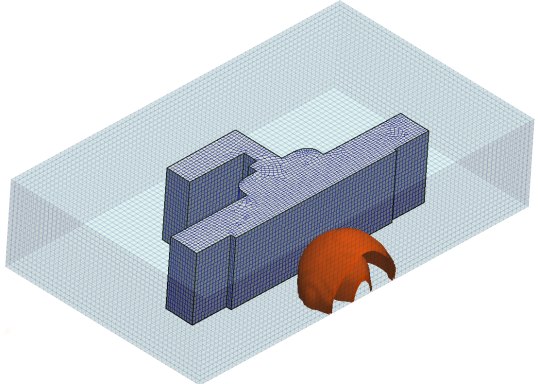
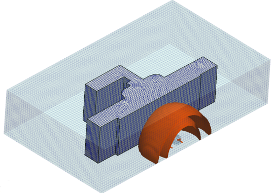
Figure 1: Blast wave propagating on the outside of a building.

2 Methodology

In the case of blast waves, the parametrised PDEs are time-dependent and non-linear and represent a transient and fast event. For such problems, the Proper Orthogonal Decomposition (POD) which relies on a linear superposition of modes, cannot approximate the solutions efficiently. The POD has been successfully employed in combination with Gaussian Process Regression (GPR) or Neural Networks (NN) to approximate the coefficients of the reduced model (e.g. Hesthaven and Ubbiali [16], Guo and Hesthaven [14]). Recent works include the application of a POD-NN method to a combustion problem (Wang et al. [37]), a hybrid projection/data-driven ROM to turbulent flows (Hijazi et al. [17], Georgaka et al. [12]) the combination of DMD and POD with interpolation to shape optimisation (Tezzele et al.[33, 34]). Recently, Lario et al. [24] proposed a method which combines the spectral POD with a recurrent neural network to reconstruct the time evolution of the reduced coefficients.

A non-linear alternative to linear ROMs consists of local ROMs, where an approximation is sought by partitioning the solution space into sub-regions and by assigning to each sub-region a local reduced-order basis. For example, Drohmann et al. [8] and Dihlmann et al. [7] used adaptive time-domain partitioning to build local ROMs. Local ROMs were developed further by Amsallem [2], who employed an unsupervised learning algorithm in order to cluster snapshots. Amsallem et al. [3] applied local ROMs in the context of hyper-reduction and Amsallem and Haasdonk [1] proposed a state-space partitioning criterion based on the true projection error instead of the Euclidean distance.

In recent years, several contributions have shown the potential of Deep Learning (DL) techniques also in the reduction stage of reduced order models. For example, Wiewel et al. [38] proposed an approach based on Convolutional Neural Networks (CNN) and Long Short-Term Memory (LSTM) to predict the temporal evolution of a physical function. Physics-Informed Neural Networks (PINN) and Physics-Reinforced Neural Networks (PRNN) have been successfully used in the data-driven solution and discovery of partial differential equations (e.g. Raissi et al. [29], Chen et al. [6]).

Another possible nonlinear and deep learning-based approach in model order reduction is based on Autoencoders. These are unsupervised artificial neural networks (ANN) able to learn a reduced representation of the given data, commonly used in image recognition and denoising (e.g. Gondara [13], Luo et al. [25]). Autoencoders have also been successfully employed in model order reduction (e.g. Nikolopoulus et al. [27], Maulik et al. [26], Romor et al. [30]). Fresca et al. [10] proposed a DL-ROM scheme, based on convolutional autoencoders, applied to PDEs representing wave-like behaviour. Applying an Autoencoder directly to the snapshots would lead to an input layer with as many neurons as degrees of freedom of the problem. This approach is feasible whenever the discrete space is not too large, and the training of ANNs in the reduction step is not excessively time-expensive. To overcome this difficulty, Phillips et al. [28] and Fresca et al. [11] employ a POD as the first reduction step, and subsequently an Autoencoder to further reduce the dimension of the problem.

To the best of our knowledge, not much work has been done on reduced order methods for blasting. For example, Xiao et al. [39] used a POD-RBF scheme for solids interacting with compressible fluid flows focusing on crack propagation.

In this work, we introduce a piecewise POD-DL scheme which combines a local POD approach and deep learning methods able to deal with fast and transient phenomena involving fluid-structure interactions such as blast waves in the vicinity of buildings. Local ROMs based on time-domain partitioning are particularly suited for problems characterised by different physical regimes and fast development, such as blast waves. We apply a first reduction layer which consists of a piecewise-POD in time, followed by an Autoencoder (AE) which works as a second non-linear reduction step. Finally, we train a Deep Forward Neural Network (DFNN) to learn the latent space dynamics. The offline procedure is summarised in Figure 2. The novelty of this work lies in the use of deep learning techniques combined with a local approach and the application to a large-scale system representing fast and transient dynamics.

2.1 Proper Orthogonal Decomposition

In this section, we revise the Proper Orthogonal Decomposition method (Benner et al.[4]). Let $u_{h}$ be a high-fidelity solution to a parametrised partial differential equation that can be written as follows

$$u_{h}(t,\mathbf{x},\boldsymbol{\mu})=\sum_{i=1}^{N_{h}}u_{h}^{(i)}(t,\boldsymbol{\mu})\*\phi_{i}(\mathbf{x}),$$

where $\{\phi_{i}\}$ represents a base of the discrete approximation space $V_{h}$ (eg. finite volume method), $N_{h}=\dim(V_{h})$ is the number of degrees of freedom, $t\in\mathcal{T}$ (time interval), $\mathbf{x}\in\Omega\subset\mathbb{R}^{3}$ (space domain) and $\boldsymbol{\mu}\in\mathcal{P}\subset\mathbb{R}^{d}$ (parameter domain). The vector $\mathbf{u}_{h}=[u_{h}^{(1)},\dots,u_{h}^{(N_{h})}]\in\mathbb{R}^{N_{h}}$ collects the coefficients of the approximation.

Figure 2: Piecewise POD-DL scheme: offline stage.

The time domain $\mathcal{T}$ is partitioned into $J$ sub-intervals $T_{j}$ such that $\mathcal{T}=\cup_{j=1}^{J}T_{j}$. Let $\mathcal{P}_{h}=\{\boldsymbol{\mu}_{j}\}_{j=1}^{N_{\mu}}$ be a sampling of the parameter space $\mathcal{P}$. We can obtain a collection of high-fidelity solutions by applying a full-order solver for different parameter values in $\mathcal{P}_{h}$ and divide them according to the time-domain partitioning. For each subset of snapshots, we apply the same procedure. For the sub-interval $T_{j}$, we build the snapshot matrix $S$ defined as follows

$$S=[S_{1},\dots,S_{N_{\boldsymbol{\mu}}}]\in\mathbb{R}^{N_{h}\times N_{s}},$$

where $N_{s}=N_{\boldsymbol{\mu}}\*N_{t}$ is the number of snapshots and $S_{k}$ is the time-trajectory matrix that collects solutions for the parameter value $\boldsymbol{\mu}_{k}$ and $t_{i}\in T_{j}$, i.e.

$$S_{k}=[\mathbf{u}_{h}(t_{1},\boldsymbol{\mu}_{k}),\dots,\mathbf{u}_{h}(t_{N_{t}},\boldsymbol{\mu}_{k})]\in\mathbb{R}^{N_{h}\times N_{t}}.$$

We seek a reduced basis approximation to the high-fidelity solution $\mathbf{u}_{h}(t,\boldsymbol{\mu})$ for $t\in T_{j}$ in the form

$$\mathbf{u}_{h,\mathrm{POD}}(t,\boldsymbol{\mu})=\sum_{i=1}^{N}{u}^{(i)}_{N}(t,\boldsymbol{\mu})\*\mathbf{v}_{i}=V\*\mathbf{u}_{N},$$ (1)

such that $N\ll N_{s}$. The vector $\mathbf{u}_{N}\in\mathbb{R}^{N}$ collects the reduced coefficients, while $\{\mathbf{v}_{i}\}$ form the basis of a reduced space $V_{\mathrm{rb}}$.

We can use the well-known POD method in order to extract an orthogonal basis. We apply a singular value decomposition to the snapshot matrix $S$, which takes the form

$$S=U\*\Sigma\*W^{T},$$

where $U,W$ are unitary matrices and $\Sigma=\text{diag}(\sigma_{1},\dots,\sigma_{r},0,\dots,0)$ is a diagonal matrix with decreasing singular values on the diagonal and rank $r\leq\min(N_{h},N_{s})$.

The basis consisting of the first $N<r$ left singular vectors of $S$ is the best approximation in the least-squares sense to the snapshots collected in $S$. The orthogonal matrix $V$, composed of the first $N$ column vectors of $U$, minimises the projection error of the snapshots over all orthogonal matrices in $\mathbb{R}^{N_{h}\times N}$, i.e.

$$\|S-V\*V^{T}\*S\|_{F}=\min_{\begin{subarray}{c}Z\in\mathbb{R}^{N_{h}\times N}\\ Z^{T}\*Z=\mathbb{I}_{I}\end{subarray}}\|S-Z\*Z^{T}\*S\|_{F}=\sum_{i=N+1}^{r}\sigma_{i}^{2},$$

with $\|\cdot\|_{F}$ being the Frobenius norm and $\mathbb{I}_{N}$ the identity matrix. Therefore, the amount of information carried by the first $N$ modes depends on the square of the singular values of the system. We can set a criterion to choose the dimension of the basis $N=\dim(V_{rb})$ such that

$$\frac{\sum^{r}_{i=N+1}\sigma_{i}^{2}}{\sum^{r}_{i=1}\sigma_{i}^{2}}\leq\epsilon,$$

for a chosen tolerance $\epsilon$. The time partitioning is determined so that the projection error in each time interval is of the same order.

2.2 Autoeconders

An Autoencoder is a type of neural network composed of two networks, where the input matches the output. One network, the encoder, is a map from the input vector $\mathbf{z}\in\mathbb{R}^{N}$ to a lower dimensional vector $f_{\mathrm{E}}(\mathbf{z})\in\mathbb{R}^{n}$, $n<N$. The second part of the network, known as the decoder, maps a low dimensional vector $f_{\mathrm{E}}(\mathbf{z})\in\mathbb{R}^{n}$ to the same dimension of the input $\mathbf{z}$, i.e. $f_{\mathrm{D}}(f_{\mathrm{E}}(\mathbf{z}))\in\mathbb{R}^{N}$. An autoencoder can be classified as a type of unsupervised learning technique since it does not require labelled data.

In this work, we exploit autoencoders in order to reduce further after the application of the POD as described in Section 2.1. Specifically, we train an autoencoder to compress the vector of reduced coefficients $\mathbf{u}_{N}=V^{T}\*S\in\mathbb{R}^{N}$ in the POD approximation defined by equation (1), to a latent space representation $\mathbf{u}_{n}\in\mathbb{R}^{n}$ with $n<N$. Once the AE is trained, we have an encoder map $f_{\mathrm{E}}$ and a decoder map $f_{\mathrm{D}}$ that can be used to find the reconstructed coefficients $\mathbf{u}_{N,\mathrm{AE}}$ as follows

$$\mathbf{u}_{N,\mathrm{AE}}=f_{\mathrm{D}}(f_{\mathrm{E}}(\mathbf{u}_{N}))\in\mathbb{R}^{N}.$$

An approximation to the full-order solution $\mathbf{u}_{h}$ for $t\in T_{j}$ can be obtained as a linear combination of the reduced basis functions, i.e.

$$\mathbf{u}_{h,\mathrm{AE}}=V\*\mathbf{u}_{N,\mathrm{AE}}\in\mathbb{R}^{N_{h}}.$$ (2)

2.3 Regression

Figure 3: Piecewise POD-DL scheme: online stage.

Finally, a regression model is used to approximate the map $\pi:\mathcal{T}\times\mathcal{P}\rightarrow\mathbb{R}^{n}$ from the time and parameter space to the latent space, defined as

$$(t,\boldsymbol{\mu})\to\pi(t,\boldsymbol{\mu})=\mathbf{u}_{n}(t,\boldsymbol{\mu}),$$

where $\mathbf{u}_{n}=f_{\mathrm{E}}(\mathbf{u}_{N})$ is the encoded representation of $\mathbf{u}_{N}$. In this work, we use a Deep Forward Neural Network (DFNN), although other choices are possible (e.g. Guo and Hesthaven [14]). Once an approximated regression map $\pi_{\mathrm{NN}}$ is obtained, for any untrained time and parameter vector $(\bar{t},\bar{\boldsymbol{\mu}})$ the approximated latent space is obtained by evaluating the regression model, i.e.

$$\mathbf{u}_{n}(\bar{t},\bar{\boldsymbol{\mu}})\approx{\mathbf{u}}_{n,\mathrm{NN}}(\bar{t},\bar{\boldsymbol{\mu}})={\pi}_{\mathrm{NN}}(\bar{t},\bar{\boldsymbol{\mu}}).$$

In the online stage, as illustrated in Figure 3, we recover an approximation of $\mathbf{u}_{h}$ as a linear combination of the POD modes, where the coefficients are obtained by applying the decoder function, $f_{\mathrm{D}}$ to the approximated latent space, as follows

$$\mathbf{u}_{h,\mathrm{POD-DL}}(\bar{t},\bar{\boldsymbol{\mu}})=V\*f_{\mathrm{D}}(\mathbf{u}_{n,\mathrm{NN}}(\bar{t},\bar{\boldsymbol{\mu}}))\in\mathbb{R}^{N_{h}}.$$ (3)

2.4 Error calculations

We can evaluate the performance of the entire scheme by calculating the error between the high-fidelity solution $\mathbf{u}_{h}$ and its approximation ${\mathbf{u}}_{h,\mathrm{POD-DL}}$, which satisfies the following inequality

$$\|\mathbf{u}_{h}-{\mathbf{u}}_{h,\mathrm{POD-DL}}\|\leq\|\mathbf{u}_{h}-{\mathbf{u}}_{h,\mathrm{POD}}\|+\|\mathbf{u}_{h,\mathrm{POD}}-{\mathbf{u}}_{h,\mathrm{AE}}\|+\|\mathbf{u}_{h,\mathrm{AE}}-{\mathbf{u}}_{h,\mathrm{POD-DL}}\|,$$

where $\|\cdot\|$ is the chosen norm in $\mathbb{R}^{N_{h}}$. In this work, we consider the $L^{1},L^{2}$ and $L^{\infty}$ vector norms. Thus, we define the relative projection error

$$\epsilon_{\mathrm{POD}}(t,\boldsymbol{\mu})=\frac{\|\mathbf{u}_{h}-\mathbf{u}_{h,\mathrm{POD}}\|}{\|\mathbf{u}_{h}\|}=\frac{\|\mathbf{u}_{h}-V\*V^{T}\*\mathbf{u}_{h}\|}{\|\mathbf{u}_{h}\|},$$ (4)

with $\mathbf{u}_{h,\mathrm{POD}}$ being the projection onto the reduced space defined by equation (1). To evaluate the performance of the Autoencoder alone, we define the relative error

$$\epsilon_{\mathrm{AE}}(t,\boldsymbol{\mu})=\frac{\|\mathbf{u}_{h,\mathrm{POD}}-{\mathbf{u}}_{h,\mathrm{AE}}\|}{\|\mathbf{u}_{h,\mathrm{POD}}\|},$$ (5)

where ${\mathbf{u}}_{h,\mathrm{AE}}$ is defined by equation (2). The relative regression error, which accounts only for the error committed by the DFNN, is defined as

$$\epsilon_{\mathrm{NN}}(t,\boldsymbol{\mu})=\frac{\|\mathbf{u}_{h,\mathrm{AE}}-{\mathbf{u}}_{h,\mathrm{POD-DL}}\|}{\|\mathbf{u}_{h,\mathrm{AE}}\|}.$$ (6)

Finally, we evaluate the entire POD-DL scheme by calculating the relative error

$$\epsilon_{\mathrm{POD-DL}}(t,\boldsymbol{\mu})=\frac{\|\mathbf{u}_{h}-{\mathbf{u}}_{h,\mathrm{POD-DL}}\|}{\|\mathbf{u}_{h}\|}.$$ (7)

3 Blast waves in urban environments

The example analysed in this work consists of an explosion occurring on the outside of a building (Figure 1). We obtain a set of snapshots by computing the time-dependent pressure field and by varying the $x$-position of the explosion.

The high-fidelity solutions are obtained with EUROPLEXUS adopting a compressed bubble model (phenomenological model) (Larcher et al. [21]) for the representation of the blast load in the fluid. The explosion is simulated by imposing an initial condition consisting of a bubble of high pressure, which expands and propagates throughout the fluid domain. The overpressure in the bubble is automatically calculated given the volume and the mass of the charge.

The air in the fluid domain is modelled as a perfect gas and discretised using a uniform mesh, where the cells have a uniform length in each direction. The compressible and inviscid (Euler) equations are solved by marching in time with an explicit second-order scheme. The building is represented by a non-deformable structure embedded in the fluid mesh and a fast search algorithm is employed to determine which fluid cells lie inside the structure’s influence domain (Casadei et al. [5]). The fluid is described by an Eulerian formulation, while the structure is described by a Lagrangian formulation. The discretisation technique for the fluid domain is a second-order cell-centred finite volume method, where all the variables are discretised at the centre of the volumes. The fluid domain consists of 66240 finite volumes with a mesh size of 2.5m. Infinite boundary conditions are applied to the surfaces of the fluid domain which interface with the open space. EUROPLEXUS is able to perform a risk analysis, which is based on the calculation of two important quantities, impulse and peak overpressure. Impulse and peak overpressure at the final time are essential quantities to the estimation of the consequences on structures and humans (Ferradas et al. [9]). Let $p_{0}$ denote the atmospheric pressure ($p_{0}=10^{5}$ Pa). Impulse and peak overpressure are defined, respectively, as

$$I(t) =\int_{0}^{t}\big{(}p(\tau)-p_{0}\big{)}_{+}\ d\tau,$$ (8)

$$p_{\mathrm{max}}(t) =\max_{\tau\in(0,t)}\big{(}p(\tau)-p_{0}\big{)}_{+},$$ (9)

where $p$ is the pressure and $(\cdot)_{+}$ represents the positive part of a function.

3.1 Problem description

For the purpose of applying the reduced order scheme introduced in Section 2, we generate a set of $N_{\mu}=30$ pressure trajectories, i.e. $\{\mathbf{u}_{h}(t_{j},\mu_{k})\}_{j,k}$, where $j\in\{1,\dots,N_{t}\}$ and $k\in\{1,\dots,N_{\mu}\}$. Since the SI is adopted by the high-fidelity solver, the pressure is expressed in Pascal while distances and time are measured in meters and seconds, respectively. From this point on, for the sake of brevity, we omit units in our results. The parameter $\mu=x_{\mathrm{exp}}$ represents the $x$-position of the explosion and the parameter space is $\mathcal{P}=[129,189]$. The space domain where the structure is submersed is $\mathcal{D}=[60,258]\times[130,245]\times[0,45]\subset\mathbb{R}^{3}$. Other fixed parameters consist of the mass of the explosive, $m_{\mathrm{exp}}=100$, the $y$- and $z$-coordinates of the explosion, $y_{\mathrm{exp}}=140$ and $z_{\mathrm{exp}}=5.5$. The high-fidelity solution $\mathbf{u}_{h}\in\mathbb{R}^{N_{h}}$ represents the pressure field with $N_{h}=66240$ degrees of freedom. Since a cell-centred finite volume scheme is employed, each component of the vector $\mathbf{u}_{h}$ represents the pressure at the centre of a cell of the fluid grid. For this problem, the number of time steps employed by the high-fidelity solver is $N_{t}=520$. As time domain, we restrict our attention to $\mathcal{T}=[0.01,0.5]$, since the air bubble for $t<0.01$ is still confined to the vicinity of the initial explosion and far from the structure. The solution at the first instants is more difficult to approximate given the high overpressure concentrated in only a few elements of fluid. The time-interval $\mathcal{T}$ is partitioned empirically, ensuring that the projection error for each sub-region is of the same order of magnitude for a particular choice of the number of modes $N$. The four sub-intervals are $T_{1}=[0.01,0.1],T_{2}=[0.1,0.2],T_{3}=[0.2,0.35],T_{4}=[0.35,0.5]$.

The encoder part of the autoencoder is composed of 7 layers with a constant decrement of neurons between each layer. For example, for $N=200$ and $n=20$, the decoder’s layers are $200\rightarrow 170\rightarrow 140\rightarrow 110\rightarrow 80\rightarrow 50\rightarrow 20$. The decoder network consists of the same layers in the reversed order. The Leaky Relu with $\alpha=0.01$ is chosen as the activation function for each layer except for the last decoding layer, where a Sigmoid function is used to ensure an output between 0 and 1. The weights are initialised using the He Normal initialiser and the optimisation algorithm is Adam Optimiser with learning rate $\lambda=10^{-4}$. As loss function, the Mean Squared Error (MSE) is used and the Mean Absolute Error (MAE) is also monitored. An Early Stopping mechanism is used, where the training stops if the loss function on a validation set does not improve over 200 epochs. The maximum number of epochs is set to 10000 and the chosen batch size is 32.

Regarding the DFNN used as a regressor from the time and parameter space to the latent space, we use 8 layers of 50 neurons each, with Sigmoid activation functions and He Normal kernel initialiser. As for the AE, the MSE is chosen as the loss function and the MAE is also monitored. The optimisation algorithm is Adam Optimiser with learning rate $\lambda=10^{-4}$, the maximum number of epochs is set to 5000, and the batch size to 32. The early stopping mechanism is used with a patience of 200 epochs.

The snapshots are divided into train, validation and test set with, respectively, $N_{\mathrm{tr}}=0.75\*N_{s}$, $N_{\mathrm{val}}=0.15\*N_{s}$ and $N_{\mathrm{te}}=0.10\*N_{s}$ number of samples. The training set is used to calculate the POD modes and train the neural networks, while the validation set is used for the Early Stopping of the neural network training. The test set is used to evaluate the scheme on untrained data.

3.2 Results

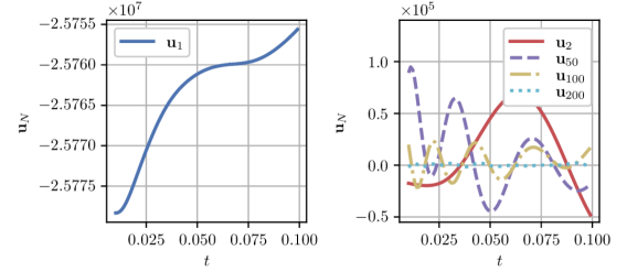
Figure 4: Reduced basis coefficients for $t\in T_{1}$, for reduced dimension $N=200$ and latent dimension $n=20$. Coefficient relative to the 1^st mode (left), and coefficients relative to the 2^nd, 50^th, 100^th and 200^th modes (right).

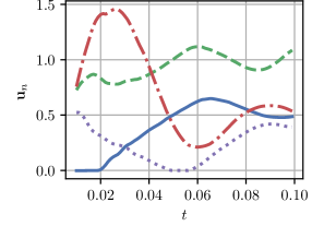
Figure 5: Time evolution of the first four latent representation vectors for reduced dimension $N=200$, latent dimension $n=20$ and for $t\in T_{1}$.

[]

[]

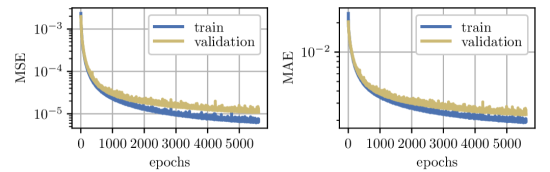
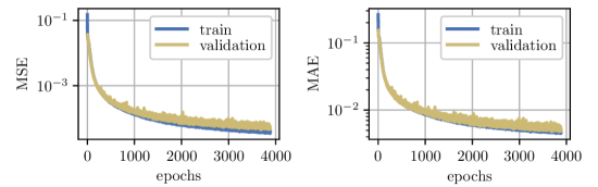
Figure 6: Training history for reduced space dimension $N=200$, latent dimension $n=20$ and $t\in T_{1}$. Training and validation MSE (loss function) on the left, training and validation MAE (monitored metric) on the right. (a) Autoencoder; (b) Deep Forward Neural Network.

In Figure 4, we show the reduced order coefficients $\mathbf{u}_{N}$ for $t\in T_{1}$ and for number of modes $N=200$ and latent dimension $n=20$. We notice that the first reduced basis coefficient $\mathbf{u}_{1}$ is two orders of magnitude higher than the second coefficient $\mathbf{u}_{2}$ for the time interval $T_{1}$. Moreover, the following coefficients decrease in magnitude and show an increasingly oscillatory behaviour. For this reason, we need to apply a suitable normalisation before training the autoencoder to ensure that all coefficients be accurately approximated. Since the first coefficient $\mathbf{u}_{1}$, relative to the dominant mode, is negative we decide to normalise it between 0 and 1 separately from the rest of the coefficients, as follows

$$\overline{\mathbf{u}}_{1}=\frac{\mathbf{u}_{1}-\min{(\mathbf{u}_{1})}}{\max{(\mathbf{u}_{1})}-\min{(\mathbf{u}_{1})}},$$

where the minimum and maximum are to be intended as calculated over all times in the training set. The remaining coefficients are normalised between 0 and 1, as follows

$$\overline{\mathbf{u}}_{N}=\frac{\mathbf{u}_{N}-\min{(\mathbf{u}_{N})}}{\max{(\mathbf{u}_{N})}-\min{(\mathbf{u}_{N})}},$$

where the minimum and maximum are calculated over all times and for all $N>2$.

The time evolution of the first four latent vectors is shown in Figure 5 for $t\in T_{1}$, for reduced dimension $N=200$ and latent space dimension $n=20$. The latent space vectors $\mathbf{u}_{n}\in\mathbb{R}^{n}$ are normalised between 0 and 1 before training the DFNN, as follows

$$\overline{\mathbf{u}}_{n}=\frac{\mathbf{u}_{n}-\min{(\mathbf{u}_{n})}}{\max{(\mathbf{u}_{n})}-\min{(\mathbf{u}_{n})}},$$

where the minimum and maximum are over all times and for all $n$.

In Figure 6, the training history for autoencoder and deep forward neural network are shown in the case where $N=200,n=20$ and $t\in T_{1}$. In Figure 6(a), we show the loss function, MSE, and the MAE in the training and validation sets for the AE network. Notice that the early stopping mechanism determines the stop of the optimisation algorithm at about 5700 epochs. In Figure 6(b), the MSE and MAE calculated in the training and validation sets for the DFNN are represented. We can observe that the optimisation stops at about 3900 epochs.

Figure 7 shows a comparison of the high-fidelity pressure field $\mathbf{u}_{h}$ and the POD-DL solution $\mathbf{u}_{\mathrm{POD-DL}}$ at $z=5$ for different times and explosion positions $(\bar{t},\bar{x}_{\mathrm{exp}})$ in the test set. The relative error is calculated as

$$\epsilon(x,y)=\frac{|\mathbf{u}_{h}-\mathbf{u}_{\mathrm{POD-DL}}|}{\mathrm{mean}{(\mathbf{u}}_{h})},$$ (10)

where the mean is over the domain at $z=5$. We notice that the POD-DL scheme is able to reconstruct the solution accurately. The errors are higher at smaller times, e.g. for $(\bar{t},\bar{x}_{\mathrm{exp}})=(0.07,170.38)$ the relative errors reach approximately $1.5\%$ while for $(\bar{t},\bar{x}_{\mathrm{exp}})=(0.4,180.72)$ they are up to $0.06\%$. At $t\approx 0.01$, the pressure wave is still confined to a small portion of the domain, where the overpressure is extremely high with respect to the rest of the domain. In this case, the solution is more difficult to approximate even when retaining a large number of modes in the POD expansion and this leads to larger errors.

In Figure 8, we present a comparison between the piecewise POD-DL scheme and the piecewise POD in reconstructing the pressure trajectory at two fixed positions in the space domain $\mathcal{D}$ for an explosion at $x_{\mathrm{exp}}=158.20$. The POD-DL trajectories $\mathbf{u}_{h,\mathrm{POD-DL}}(t)$ are reconstructed by applying the reduced scheme as described by equation (3) for the same time steps used by the FOM to obtain $\mathbf{u}_{h}(t)$. Note that $\mathbf{u}_{h,\mathrm{POD}}$ represents the projected solution, i.e. $\mathbf{u}_{h,\mathrm{POD}}=V\*V^{T}\*\mathbf{u}_{h}$, without any regression or interpolation of the reduced coefficients. Therefore, it represents the best that can be obtained with the POD method, without accounting for the errors introduced by reconstructing the coefficients from the parameter space. We can see that the scheme hereby proposed with $N=200$ and $n=20$ performs considerably better compared to a piecewise POD with $N=20$ modes per each time interval. For a point located near the left corner of the building $(x,y,z)=(150,100,5.5)$, the overpressure reaches about $3000$ Pa and the $L^{2}$-error in time amounts to 17.30 for the piecewise POD scheme and 5.07 for the piecewise POD-DL scheme. For $(x,y,z)=(200,200,5.5)$ located behind the building, the overpressure amounts to $200$ Pa and the $L^{2}$-error in time is equal to 0.67 for the piecewise POD scheme and to 0.20 for the piecewise POD-DL scheme.

In this particular case, the time employed by EUROPLEXUS to compute one trajectory is approximately $445s$, while the ROM method described in Section 2 requires about $0.2s$ to compute an approximated solution in the online phase. It is important to notice that, the latter refers to the time required to obtain an approximated solution for given values of the time and $x-$position of the explosion. In order to obtain the time required to compute the whole trajectory, it is necessary to multiply it by the appropriate number of timesteps.

[]

[]

[]

[]

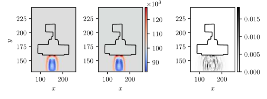
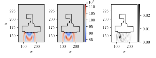
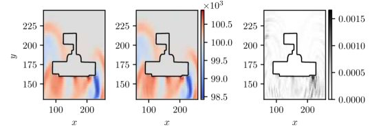
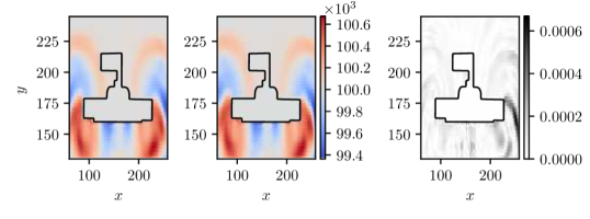
Figure 7: Comparison between high-fidelity pressure field, $\mathbf{u}_{h}$ (left), and POD-DL solution, $\mathbf{u}_{h,\mathrm{POD-DL}}$ (centre), using $N=200$, $n=20$. Relative error on the right. At (a) $(\bar{t},\bar{x}_{\mathrm{exp}})=(0.07,170.38)$; (b) $(\bar{t},\bar{x}_{\mathrm{exp}})=(0.1,131.07)$; (c) $(\bar{t},\bar{x}_{\mathrm{exp}})=(0.2,160.03)$; (d) $(\bar{t},\bar{x}_{\mathrm{exp}})=(0.4,180.72)$.

3.2.1 Impulse and Overpressure

In Figure 10, we show the impulse and overpressure for an explosion located at $x_{\mathrm{exp}}=158.20$, at the final time $t=0.5$ and a height of $z=5$ from the ground. Impulse and overpressure are calculated from the pressure trajectory using equations (8)-(9). We compare the high-fidelity solutions $\mathbf{I}_{h},\mathbf{p}_{\mathrm{max},h}$ with the reduced solution $\mathbf{I}_{\mathrm{POD-DL}},\mathbf{p}_{\mathrm{max},\mathrm{POD-DL}}$ computed with $N=200$ and $n=20$ and we calculate the error as done for the pressure field, using equation (10). We can see, from Figure 10(a), that for the impulse the relative errors amount to 0.75 in some areas of the domain. In Figure 10(b), the relative errors in reconstructing the overpressure reach 7.5 in the vicinity of the original explosion.

Figure 10 represents the impulse and overpressure at $t=0.5$ and at a fixed $y=160$, which corresponds to the front facade of the building. The error between high-fidelity and reduced solutions ($N=200,n=20$) is calculated using equation (10), where the mean is calculated over the domain at $y=160$. The errors are at most $15\%$ for the impulse and $20\%$ for the overpressure.

In Figure 11, we compare the trajectories of impulse and overpressure for an explosion position $x_{\mathrm{exp}}=158.20$ at two different positions in the domain, $(x,y,z)=(100,150,5.5)$ located near the left corner of the building and at $(x,y,z)=(200,200,5.5)$, located behind the building.

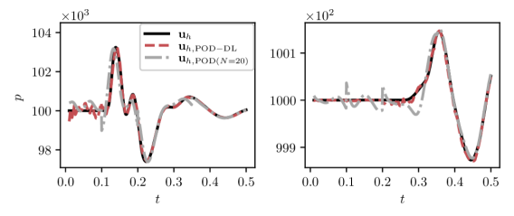
Figure 8: High-fidelity pressure trajectory $\mathbf{u}_{h}$, piecewise POD solution $\mathbf{u}_{h,\mathrm{POD}}$ with $N=20$ and POD-DL trajectory $\mathbf{u}_{h,\mathrm{POD-DL}}$ obtained with $N=200$ and $n=20$ for $x_{\mathrm{exp}}=158.20$, at two fixed positions in the space domain. At $(x,y,z)=(100,150,5.5)$ (left), $L^{2}$-error in time for POD: 17.30, for POD-DL: 5.07. At $(x,y,z)=(200,200,5.5)$ (right), $L^{2}$-error in time for POD: 0.67, for POD-DL: 0.20.

[]

[]

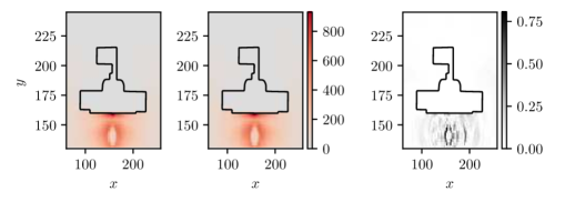
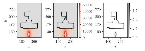
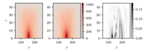
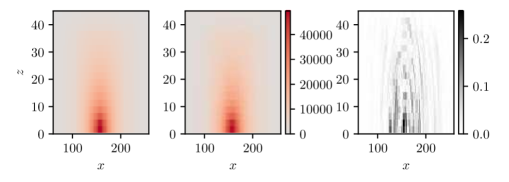
Figure 9: Comparison of the high-fidelity solution (left) and the reduced solution (centre) using $N=200$ and $n=20$ at $z=5$, for $\bar{x}_{\mathrm{exp}}=158.20$, and relative error (right). (a) Impulse at $t=0.5$; (b) Peak Overpressure at $t=0.5$.

[]

[]

Figure 10: Comparison of the high-fidelity solution (left) and the reduced solution (centre) using $N=200$ and $n=20$ on the front facade ($y=160$) of the building, for $\bar{x}_{\mathrm{exp}}=158.20$, and relative error (right). (a) Impulse at $t=0.5$; (b) Peak Overpressure at $t=0.5$.

[]

[]

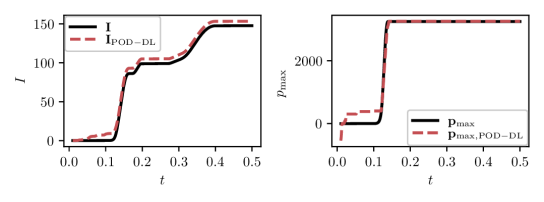
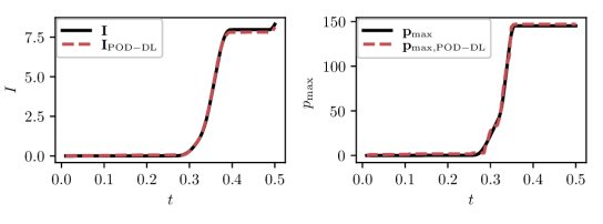
Figure 11: Comparison of the FOM and the POD-DL trajectories using $N=200$ and $n=20$, for $x_{\mathrm{exp}}=158.20$. (a) Impulse (left) and Peak Overpressure (right) at $(x,y,z)=(100,150,5.5)$; (b) Impulse (left) and Peak Overpressure (right) at $(x,y,z)=(200,200,5.5)$.

3.2.2 Error analysis

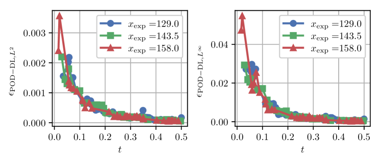
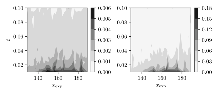
Figure 12: Errors against time in $L^{2}$ (left) and $L^{\infty}$ norm (right) between the high-fidelity solution $\textbf{u}_{h}$ and the reduced solution $\textbf{u}_{\mathrm{POD-DL}}$ for $N=200$, $n=20$ and different values of $x_{\mathrm{exp}}$.

Figure 13: Errors in a $x_{\mathrm{exp}}t$ plane between the high-fidelity solution $\textbf{u}_{h}$ and the reduced solution $\textbf{u}_{\mathrm{POD-DL}}$ for $N=200$ and $n=20$, using the $L^{2}$ norm (left) and the $L^{\infty}$ norm (right).

In Figure 13, we present the error $\epsilon_{\mathrm{POD-DL}}$, defined by equation (7), as it varies with time and calculated in the test set for different values of $x_{\mathrm{exp}}$. We notice that, as already seen in Figure 7, the errors in $L^{2}$ and $L^{\infty}$ norm are considerably larger near $t\approx 0.01$. Moreover, the errors for $x_{\mathrm{exp}}=159$ are larger than the errors for $x_{\mathrm{exp}}=129$. This behaviour can be observed also in Figure 13, where the $L^{2}$ and $L^{\infty}$ norm errors are shown in a $x_{\mathrm{exp}}t$ plane. The errors in the middle of the parameter space $\mathcal{P}=[129,189]$ are larger than at the boundaries of the parameter space.

In Figure 15, we split the various sources of error to look at how they contribute to the global error $\epsilon_{\mathrm{POD-DL}}$, given by equation (7). We plot separately the POD error $\epsilon_{\mathrm{POD}}$, defined by equation (4), the error given by the autoencoder $\epsilon_{\mathrm{AE}}$, defined by equation (5), and the error given by the neural network employed as regressor $\epsilon_{\mathrm{NN}}$, defined by equation (6). We notice that all the components of the errors are larger at $t\approx 0.1$ and that the autoencoder is the greatest source of error.

We perform an error analysis to investigate the performance of the piecewise POD-DL scheme, varying the number of modes $N$ retained in the POD expansion and the latent dimension $n$. First, we vary the reduced space dimension $N$ from 25 to 200, while keeping fixed the latent dimension to $n=20$. We plot the different components of error in $L^{1},L^{2}$ and $L^{\infty}$ norm. We note that all the errors decay as $N$ increases. In particular, the $L^{2}$ POD error, $\epsilon_{\mathrm{POD}}$, is approximately $0.2\%$ for $N=25$ and decreases to about $0.01\%$ for $N=200$. The AE error in $L^{2}$ norm, $\epsilon_{\mathrm{AE}}$, improves slightly from $0.1\%$ for $N=25$ to about $0.05\%$ for $N=200$. As $N$ increases, there is an increasing amount of information that the autoencoder compresses to a latent space of dimension $n=20$. The NN error in $L^{2}$ norm, $\epsilon_{\mathrm{NN}}$, sees a slight improvement over $N$ since the latent space reconstructed from the time and parameter space has a fixed dimension $n=20$. Finally, the global error in $L^{2}$ norm, $\epsilon_{\mathrm{POD-DL}}$, decreases until about $0.05\%$ for $N=125$. For larger reduced dimensions, there is no significant improvement.

Figure 17 shows how errors vary with latent dimension $n$, while keeping constant the number of modes $N=200$. In this case, the errors introduced by the POD projection, $\epsilon_{\mathrm{POD}}$, remain constant. The AE errors, $\epsilon_{\mathrm{AE}}$, decay until about $n=20$ and flatten for larger values of $n$. The errors introduced by the regression, $\epsilon_{\mathrm{NN}}$, decay until about $n=20$ and then slowly increase with $n$. This is because a larger latent space is more difficult to reconstruct from the time and parameter space. The global error, $\epsilon_{\mathrm{POD-DL}}$, decreases until about $n=20$. For larger values of $n$, there is no improvement.

Figure 17 shows the projection error, $\epsilon_{\mathrm{POD}}$, with increasing number of modes $N$ and the POD-DL error, $\epsilon_{\mathrm{POD-DL}}$, with fixed $N=200$ and increasing latent dimension $n$. We can see how the POD-DL scheme leads to smaller errors in both $L^{2}$ and $L^{\infty}$ norm. In particular, $\epsilon_{\mathrm{POD-DL}}$ with $N=200,n=20$ is one order of magnitude smaller than $\epsilon_{\mathrm{POD}}$ with $N=20$.

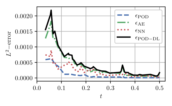
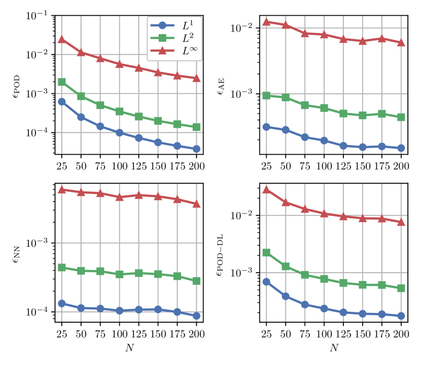
Figure 14: Different components of error in $L^{2}$ norm against time for $N=200,n=20$ and $\bar{x}_{\mathrm{exp}}=129$.

Figure 15: Errors against the reduced space dimension $N$ for a fixed value of latent dimension $n=20$.

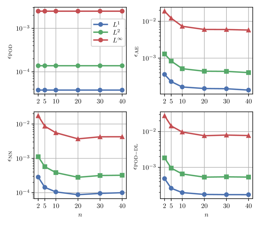
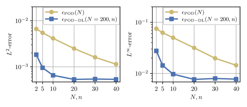
Figure 16: Errors against the latent dimension $n$ for a fixed value of reduced space dimension $N=200$.

Figure 17: Comparison between POD errors against $N$ and POD-DL errors against $n$ for a fixed $N=200$, in $L^{2}$ norm (left) and $L^{\infty}$ norm (right).

4 Conclusions

In this work, we proposed a local and non-linear Reduced Order Method able to efficiently approximate the fast evolution of blast waves. This kind of problems requires the solution of non-linear and time-dependent parametric PDEs and is characterised by a large scale and fast and transient development. The validity of the method is shown in an example consisting of a blast wave propagating near a building. A set of snapshots are obtained by varying the $x$-component of the explosion position.

The scheme hereby proposed is based on a local approach, where the snapshots are divided following a time-domain partitioning and a local-reduced order basis is built for each sub-region. The reduced order spaces are generated using the POD and by retaining a large number $N$ of modes. The POD method alone is not able to represent the solutions efficiently since the singular values decay very slowly for this type of problems. Therefore, the remarkable compression capabilities of autoencoders are exploited to build a latent space of dimension $n<N$. A regression map between the time and parameter space and the latent space is then approximated using a deep forward neural network.

We showed that, for new values of the time and parameter, the piecewise POD-DL method leads to very accurate approximations of the pressure field. Moreover, it performs considerably better in reconstructing the pressure trajectories compared to the POD method. Then, we tested the method in approximating the impulse and peak overpressure fields at the final time.

Finally, we performed an error analysis. We presented the $L^{2}$ and $L^{\infty}$ norm errors as they vary with time and showed that the greatest errors are for $t\approx 0$ as expected. The solutions at smaller times consist of a high-pressure bubble confined to a small region. This causes difficulties for the POD to approximate the solutions even when retaining a high number of modes. We analysed errors by varying the number of modes $N$ and the latent dimension $n$. We proved that errors decrease when increasing the value of $N$ and keeping the latent space dimension fixed. Also, the errors decay when increasing $n$ and fixing the reduced space dimension. However, at about $n\approx 20$ the errors flatten due to the regression with DFNN.

It is important to notice that the computational cost to recreate one particular time step with the ROM method (equal to approximately $0.2\text{s}$) would not change significantly even if a large-scale model was employed. On the contrary, the computational cost for a simulation with EUROPLEXUS (or another implicit code) would become much more expensive as the size of the discretisation increases. That makes the proposed approach suitable for a fast (even real-time) solution once the model has been trained even for a large-scale problem.

In terms of future perspectives, we aim to test the developed methodology also for different physics and verify the applicability of the compression strategy for the development of projection-based ROMs [32, 30]. Moreover, possible improvements are in the direction of studying unsupervised learning strategies to identify clusters of solution into both the solution space, the parameter space and the time domain.

References

- [1] Amsallem, D., and Haasdonk, B. PEBL-ROM: Projection-error based local reduced-order models. Advanced Modeling and Simulation in Engineering Sciences 3, 6 (2016).
- [2] Amsallem, D., Zahr, M. J., and Farhat, C. Nonlinear model order reduction based on local reduced-order bases. International Journal for Numerical Methods in Engineering 92, 10 (2012), 891–916.
- [3] Amsallem, D., Zahr, M. J., and Washabaugh, K. Fast local reduced basis updates for the efficient reduction of nonlinear systems with hyper-reduction. Advances in Computational Mathematics 41, 5 (2015), 1187–1230.
- [4] Benner, P., Grivet-Talocia, S., Quarteroni, A., Rozza, G., Schilders, W., and Silveira, L. M., Eds. Model Order Reduction: Volume 2: Snapshot-Based Methods and Algorithms. De Gruyter, 2020.
- [5] Casadei, F., Larcher, M., and Leconde, N. Strong and weak forms of a fully non-conforming FSI algorithm in fast transient dynamics for blast loading of structures. In COMPDYN 2011 Proceedings of the 3rd International Conference on Computational Methods in Structural Dynamics and Earthquake Engineering (2012), M. Papadrakakis, M. Fragiadakis, and V. Plevris, Eds., National Technical University of Athens, pp. 1120–1139.
- [6] Chen, W., Wang, Q., Hesthaven, J. S., and Zhang, C. Physics-informed machine learning for reduced-order modeling of nonlinear problems. Journal of Computational Physics 446 (2021), 110666.
- [7] Dihlmann, M., Drohmann, M., and Haasdonk, B. Model reduction of parametrized evolution problems using the reduced basis method with adaptive time partitioning. In ECCOMAS Thematic Conference - ADMOS 2011: International Conference on Adaptive Modeling and Simulation, An IACM Special Interest Conference (2012), D. Aubry and P. Díez, Eds., pp. 156–167.
- [8] Drohmann, M., Haasdonk, B., and Ohlberger, M. Adaptive Reduced Basis Methods for Nonlinear Convection-Diffusion Equations. Springer Proceedings in Mathematics 4 (2011), 369–377.
- [9] Ferradás, E. G., Alonso, F. D., Miñarro, M. D., Aznar, A. M., Gimeno, J. R., and Pérez, J. F. S. Consequence analysis by means of characteristic curves to determine the damage to humans from bursting spherical vessels. Process Safety and Environmental Protection 86, 2 (2008), 121–129.
- [10] Fresca, S., Dedé, L., and Manzoni, A. A Comprehensive Deep Learning-Based Approach to Reduced Order Modeling of Nonlinear Time-Dependent Parametrized PDEs. Journal of Scientific Computing 87, 61 (2021), 1–36.
- [11] Fresca, S., and Manzoni, A. POD-DL-ROM: Enhancing deep learning-based reduced order models for nonlinear parametrized PDEs by proper orthogonal decomposition. Computer Methods in Applied Mechanics and Engineering 388 (2022), 114181.
- [12] Georgaka, S., Stabile, G., Star, K., Rozza, G., and Bluck, M. J. A hybrid reduced order method for modelling turbulent heat transfer problems. Computers & Fluids 208 (2020), 104615.
- [13] Gondara, L. Medical Image Denoising Using Convolutional Denoising Autoencoders. In IEEE 16th International Conference on Data Mining Workshops (ICDMW) (2016), Institute of Electrical and Electronics Engineers, pp. 241–246.
- [14] Guo, M., and Hesthaven, J. S. Data-driven reduced order modeling for time-dependent problems. Computer Methods in Applied Mechanics and Engineering 345 (2019), 75–99.
- [15] Hesthaven, J. S., Rozza, G., and Stamm, B. Certified Reduced Basis Methods for Parametrized Partial Differential Equations. Springer Briefs in Mathematics. Springer, Switzerland, 2015.
- [16] Hesthaven, J. S., and Ubbiali, S. Non-intrusive reduced order modeling of nonlinear problems using neural networks. Journal of Computational Physics 363 (2018), 55–78.
- [17] Hijazi, S., Stabile, G., Mola, A., and Rozza, G. Data-driven POD-Galerkin reduced order model for turbulent flows. Journal of Computational Physics 416 (2020), 109513.
- [18] Joint Research Centre and Commissariat à l’Énergie Atomique et aux Énergies Alternatives. EUROPLEXUS. http://www-epx.cea.fr/, Accessed: 2022-09-14.
- [19] Karlos, V., Solomos, G., and Larcher, M. Analysis of the blast wave decay coefficient using the Kingery-Bulmash data. International Journal of Protective Structures 7 (2016), 409–429.
- [20] Larcher, M., Arrigoni, M., Bedon, C., Van Doormaal, A., Haberacker, C., Hus̈ken, G., Millon, O., Saarenheimo, A., Solomos, G., Thamie, L., Valsamos, G., Williams, A., and Stolz, A. Design of blast-loaded glazing windows and facades: A review of essential requirements towards standardization. Advances in Civil Engineering (2016), 2604232.
- [21] Larcher, M., and Casadei, F. Explosions in Complex Geometries — A Comparison of Several Approaches. International Journal of Protective Structures 1 (2010), 169–195.
- [22] Larcher, M., Solomos, G., Casadei, F., and Gebbeken, N. Experimental and numerical investigations of laminated glass subjected to blast loading. International Journal of Impact Engineering 39 (2012), 42–50.
- [23] Larcher, M., Valsamos, G., and Karlos, V. Access control points: Reducing a possible blast impact by meandering. Advances in Civil Engineering (2018), 3506892.
- [24] Lario, A., Maulik, R., Schmidt, O. T., Rozza, G., and Mengaldo, G. Neural-network learning of SPOD latent dynamics. Journal of Computational Physics 468 (2022), 111475.
- [25] Luo, W., Li, J., Yang, J., Xu, W., and Zhang, J. Convolutional sparse autoencoders for image classification. IEEE Transactions on Neural Networks and Learning Systems 29, 7 (2018), 3289–3294.
- [26] Maulik, R., Lusch, B., and Balaprakash, P. Reduced-order modeling of advection-dominated systems with recurrent neural networks and convolutional autoencoders. Physics of Fluids 33, 3 (2021), 037106.
- [27] Nikolopoulos, S., Kalogeris, I., and Papadopoulos, V. Non-intrusive Surrogate Modeling for Parametrized Time-dependent PDEs using Convolutional Autoencoders. Engineering Applications of Artificial Intelligence 109 (2022), 104652.
- [28] Phillips, T. R. F., Heaney, C. E., Smith, P. N., and Pain, C. C. An autoencoder-based reduced-order model for eigenvalue problems with application to neutron diffusion. International Journal for Numerical Methods in Engineering 122, 15 (2021), 3780–3811.
- [29] Raissi, M., Perdikaris, P., and Karniadakis, G. E. Physics-informed neural networks: A deep learning framework for solving forward and inverse problems involving nonlinear partial differential equations. Journal of Computational Physics 378 (2019), 686–707.
- [30] Romor, F., Stabile, G., and Rozza, G. Non-linear manifold ROM with Convolutional Autoencoders and Reduced Over-Collocation method. Submitted (2022).
- [31] Solomos, G., Larcher, M., Valsamos, G., Karlos, V., and Casadei, F. A survey of computational models for blast induced human injuries for security and defence applications. Tech. rep., European Commission Joint Research Centre, Ispra, Italy, 2020.
- [32] Stabile, G., and Rozza, G. Finite volume POD-Galerkin stabilised reduced order methods for the parametrised incompressible Navier–Stokes equations. Computers & Fluids 173 (2018), 273–284.
- [33] Tezzele, M., Demo, N., and Rozza, G. Shape optimization through proper orthogonal decomposition with interpolation and dynamic mode decomposition enhanced by active subspaces. In MARINE 2019: VIII International Conference on Computational Methods in Marine Engineering (2019).
- [34] Tezzele, M., Demo, N., Stabile, G., Mola, A., and Rozza, G. Enhancing CFD predictions in shape design problems by model and parameter space reduction. Advanced Modeling and Simulation in Engineering Sciences 7, 1 (2020).
- [35] Valsamos, G., Casadei, F., Solomos, G., and Larcher, M. Risk assessment of blast events in a transport infrastructure by fluid-structure interaction analysis. Safety Science 118 (2019), 887–897.
- [36] Valsamos, G., Larcher, M., and Casadei, F. Beirut explosion 2020: A case study for a large-scale urban blast simulation. Safety Science 137 (2021), 105190.
- [37] Wang, Q., Hesthaven, J. S., and Ray, D. Non-intrusive reduced order modeling of unsteady flows using artificial neural networks with application to a combustion problem. Journal of Computational Physics 384 (2019), 289–307.
- [38] Wiewel, S., Becher, M., and Thuerey, N. Latent Space Physics: Towards Learning the Temporal Evolution of Fluid Flow. Computer Graphics Forum 38, 2 (2019), 71–82.
- [39] Xiao, D., Yang, P., Fang, F., Xiang, J., Pain, C. C., Navon, I. M., and Chen, M. A non-intrusive reduced-order model for compressible fluid and fractured solid coupling and its application to blasting. Journal of Computational Physics 330, October (2017), 221–244.