Conformal Dilaton-Higgs Gravity on Warped Spacetimes: Black Hole Paradoxes Revisited

Abstract

We investigate on a Randall-Sundrum warped spacetime, a Kerr-like black hole in the conformal dilaton-Higgs $(\omega,\Phi)$ gravity model. We applied the antipodal boundary condition on the Klein surface using the $\mathds{Z}_{2}$-symmetry in the "large" (bulk) extra dimension. It turns out that the pseudo-Riemannian 5D manifold can be written as an effective 4D Riemannian brane spacetime, $\mathds{R}^{2}_{+}\times\mathds{R}^{1}\times S^{1}$, where $\mathds{R}^{2}_{+}$ is conformally flat. The solution in valid on both manifolds. So the solution can equally well described by an instanton solution. An advantage is that antipodicity can be maintained without a "cut-and-past" method or to rely on quantum cloning, when treating the scattering description of the evaporation process of the Hawking radiation. We need the windingnumber as quantum number. Moreover, the equations are invariant under time reversal. The problem of finding the matching condition of the near-horizon approximation and the far-away Regge-Wheeler approximation, can possibly be solved by splitting the spacetime in a dilaton field times an "un-physical" spacetime, which is conformally flat. In the case of a constant gauge field, we find that the conform invariant mass term $\sim\Phi^{2}\omega^{2}$ in the Lagrangian follows directly from the superfluous dilaton equation by suitable choice of the scale of the extra dimension. Finally, we bring forward the relation between the embedded Klein surface in $\mathds{R}^{4}$ and the quantum mechanical information paradox.

1 Introduction

One of the most profound unsolved problems in theoretical physics is the discrepancy between quantum mechanics (QM) and general relativity theory (GRT). One should like to obtain a consistent theory of quantum gravity, a major goal of theoretical physics (the "holy grail") that would reconcile QM and Einstein’s GRT. It is conjectured that the problem how to handle quantum-gravity effects, will be found near the horizon of black holes.

Back holes are in quite another perspective, incredibly unique and fascinating objects. The black hole can take part in the weird and wonderful behavior of QM. Particles can be in the quantum superposition of multiple states. They will be entangled until observers will act on the system (¨collapse of the wavefunction¨). So new Planck scale physics should be necessary to address the information paradox, complementarity and to avoid the firewall.

During the last decades, several authors proposed different approaches in order to attack this epic problem. Pioneer work was delivered by Hawkinghawking1975 , who investigated particle creation near the horizon of a black hole. He found that black holes radiate as black bodies with a thermal spectrum. So the black hole would be in a mixed state. However, this seems to suggest violation of unitary evolution, because all information connected with the in-falling particle (¨in-state¨), appears to have lost after the evaporation of the black hole. In quantum field theory (QFT) one usually deals with pure quantum states which evolve unitarily. A possible solution was addressed by Almheiri, et al.,alm2013 , in order to solve the conflict between complementarity and firewalls. The in-falling observer would burn up at the horizon´s firewall. However, this viewpoint conflicts GRT. Maldacena, et al,maldacena2013 proposed the ¨ER = EPR¨ hypothesis, which is based on the suggestion that connectivity in spacetime is equivalent to quantum entanglement. They assert that quantum entanglement of distant black holes is equivalent to the existence of an Einstein-Rosen bridge connecting them. However, one ignores the gravitational interaction between the two regions I and II in the Penrose diagram. Also the emergence of string theory, holography and gauge-gravity duality could shed light on this problem. However, the information retrieval process is not quite clearmathur2009 . Recent investigation by Foo, et al.foo2021 , suggests that even so-called “spacetime superpositions” could exist, i.e., that quantum superpositions of different spacetimes not related by a global coordinate transformation could be possible.

In general, one can state that in all these models the dynamical back reaction is ignored. For example, the evaporation process will have an impact on the near-horizon spacetime. There will be a strong interaction between, for example, a scalar field and the gravitation degrees of freedombetz2021 .

The departure from Hawking‘s calculations, leads to quantum mechanical scattering algebra, realized by in- and out-going wave functions near the horizonthooft2015 . Later, it was argued that one can reformulate this departure, by considering soft graviton exchange between matter fields near the horizon. Away from the horizon, one can then introduce an effective Regge-Wheeler gravitational potential. However, in all these models, the calculations on the quasi-normal modes were done on a fixed Schwarzschild background geometry, which is nor adequate for black hole evaporation process: the potential is time dependent. One should like to obtain a complete scattering description for the outside observer, which is consistent with the local observer.

This complementarity issue, which means the discrepancy between the local observer and the far away observer, can be reformulated in conformal dilaton gravity (CDG) by introducing a dilaton field $\omega$ and by writing $g_{\mu\nu}=\omega^{\frac{4}{d-2}}\tilde{g}_{\mu\nu}$thooft2015c . Different observers experience different notions of $\omega$, i.e., the scale of spacetime. Moreover, $\omega$ (and a scalar field $\Phi$) and $\tilde{g}_{\mu\nu}$ are invariant under $\tilde{g}_{\mu\nu}\rightarrow\Omega^{\frac{4}{d-2}}\tilde{g}_{\mu\nu},\omega\rightarrow\Omega^{-\frac{d-2}{2}}\omega,\Phi\rightarrow\Phi^{-\frac{d-2}{2}}\omega$. $\Omega$ can be used, for example, to make Ricci scalar for the local observer zero. Further, one observer sees Hawking radiation as matter, while on other one as part of his vacuum. The in-falling observer will not notice any change in the mass of the black hole. The out side observer, on the other hand, observes a gradually shrinking mass. It is conjectured that this conformal description will be necessary in order understand the black hole paradoxes.

The approach we will address in this manuscript, relies on the antipodal boundary condition on a warped 5D Spacetime. This idea was introduces decades ago by Schrödingerschrod1957 . It is sometimes called the elliptic interpretation of spacetime. Interesting investigation on this mapping where done by Sanchez, et al.san1987 ; san1988 ; fol1987 on a AdS spacetime. The model was intensively extended by´t Hooftthooft2016 ; thooft2018b ; thooft2019 in a slightly different setting, by considering a new treatment of the gravitational back-reaction. In brief, antipodal points on the horizon represent the same world-point or event. The spacetime inside the horizon is removed such that the edges are glued together by identifying the antipodes. In the language of a Penrose diagram, "region II" is the antipode of "region I".

In order to avoid wormhole constructions or demanding "an other universe" in the Penrose diagram, it is essential that the asymptotic domain of the manifold maps one-to-one onto the ordinary spacetime in order to preserve the metric. In fact, one deals with one black hole. ´t Hooft performed calculations on the unitary evolution matrix by using the antipodal boundary condition, i.e., the transverse spherical coordinates $(\theta,\varphi)$ at region II, represent the antipode of region I. So there are no fixed points. In fact, there is no "hidden" sector in the Penrose diagram. The resulting Hartle-Hawking vacuum state remains a pure state in stead of a thermodynamically mixed state for the outside observer. The Hawking particles are emerging from I, are maximally entangled with particles emerging from II. This approach has the potential to solve the information paradox and a firewall is not necessary. The antipodal boundary condition, minimizes the number of unconventional assumptions or to rely on full string theory and ¨fuzzyballs". It will require that the local laws of physics are invariant across the black hole boundarythooft2021 . Usually, one considers the Hawking particles as excitations of low energy particles that fulfill the standard model and applies perturbative quantum gravity on a fixed background metric (i.e., the gravitons). The distant observer notices the Hilbert space of low energy particles at given time. One then maps the states at later times, 1 on 1 on earlier times. One basically bypasses the Planck-area. It manifests itself only by the higher modes of the spherical harmonics (in the angle variables). An unitary S matrix can then be constructed if one applies a cut-off for the higher modes of the harmonics. In a recent study,´t Hooftthooft2022 tries to avoid the antipodal boundary condition, in order to overcome some inconsistencies, into a quantum clone description, in spherical symmetric case.

In our 5D warped spacetime, however, this change is not necessary, due to the cylindrical symmetry of the Kerr-type spacetime we considered. It is strongly conjectured that the center of galaxies harbors a spinning Kerr black holes and not a Schwarzschild black hole. So there is a preferred direction, i.e., the $z$-axis. If one omits the $dz^{2}$, one obtains the well known exact Ban̆ados-Teitelboim-Zanelli (BTZ) black hole solution in $(2+1)$-dimensional spacetimebanadoz1992 ; slagter2019b .

In the recently found vacuum solutionslagter2022c , no further inconsistency was encountered, because we had only to deal with the gravitational freedom, i.e., the dilaton field $\omega$, which was solved exactly.

In the present case, the scalar field will be written as $\Phi=\eta X(t,r)e^{in\varphi}Y_{m}(\varphi)$ and with the gauge field $A\sim\frac{n}{e}$. In order find a consistent description of the antipodal map, the warped fifth dimension is mandatory, in order to apply the non-orientable Klein surface.

In our model we will also try to avoid in the dynamical evolution of the fields (scalar, dilaton and metric components) on the Kerr spacetime, the late-times and early-times behavior, by writing the PDE´s in Kruskal coordinates

We know that local QFT and GRT are invariant under CPT transformations. In the model we consider here, we advocate that antipodal map preserves also CPT. The basic argument being that CPT is an exact symmetry of nature, i. e., of QFT around flat background. It has the potential to be elevated to a form of discrete gauge symmetry in a full theory of quantum gravity. One says that region II is a CPT-transformed quantum copy of region I.

There are some other approaches to this invariance. The conformal group implies Poincaré invariance and so PT invariancemannheim2013 . The PT symmetry would be a necessary and sufficient condition for unitary time evolution whereas hermiticity is only a sufficient condition. Dropping the hermiticity in favor of PT symmetry is not generally accepted (see also the discussion by Betzios, et al.bet2016 ; bet2017 and references therein).

There are several reasons for considering a warped spacetime of Randall and Sundrum (RS)ran1999a ; ran1999b . The recently found exact solution of the Kerr-like spacetime without a scalar field, was found in the CDG model on a warped RS spacetimeslagter2018 ; slagter2021 ; slagter2022b ; slagter2022c . These so-called brane-world models provide a simplification of the full string model. In the later string models, the extra dimensions are compactified or fold in on themselves in many ways, meaning that there are to many possible solutions to be able to make a clear prediction. In the RS model, only gravity can propagate into the bulk, while all other fields resides on the brane. Einstein gravity on the brane will be modified by the very embedding itself and opens up a possible new way to address the dark energy problemmann2005 . In a former studyslagterpan2016 we applied this model on a Friedmann-Lemaître-Robertson-alker (FLRW) spacetime. There is a contribution from the projected 5D Weyl tensor on the effective 4D brane, which carries information of the gravitational field outside the brane. If one writes the 5D Einstein equation in CDG setting, it could be possible that an effective theory can be constructed without an UV cutoff, because the fundamental scale $M_{5}$ can be much less than the effective scale $M_{Pl}$ due to the warp factor. The physical scale is therefore not determined by $M_{Pl}$. There are some other arguments which advocate for the 5D model. First, the warped model could possibly solve the hierarchy problem. Secondly, the description of the antipodal boundary condition by means of the Möbius strip in the 4D model, can be extended by considering the Klein surface, which can be embedded in $\mathds{R}^{4}$. Quite recently, Maldacena, et al.maldacena2021 , found an interesting wormhole solution on the RS model. It is remarkable that the found exact spacetime solution $\tilde{g}_{\mu\nu}$ together with the dilaton solution, is the same for the 5D and effective 4D Einstein equations. In a covariant approach of the model, it is mandatory to solve these equations together in order to obtain consistencyshirom2000 ; shirom2003 . Moreover, it turns out that the solution can be maintained, when one switches to the Riemannian 5D spacetime (Wick rotation). This instanton solution can then be embedded in $\mathds{R}^{4}$, i.e., our effective brane in the RS model. This becomes clear when one complexifies the space as $\mathds{C}^{1}\times\mathds{C}^{1}$. By the Hopf fibration, one then makes the connection with our real space.

As already mentioned, the BTZ solution shares some features with the 4D Kerr solution and gained new interest because it can be used to study quantum gravity issues. The model needs a cosmological constant and is asymptotically AdS. The relation with the dynamical "uplifted"" BTZ solution was presented by Slagterslagter2019b . After the discovery of the AdS/CFT correspondence, the BTZ solution gained new interest and became a tool to understand black hole entropy. It is not yet clear whether pure 3D Einstein gravity make sense quantum mechanically without string theory embedding. Adding a scalar field will make the model more realistic. The improvement of the treatment of the gravitational interaction of the propagating modes on a Schwarzschild background was done by Betzios, et al.betz2021 . They distinguish two regions. Far from the horizon the propagating fields evolve semi-classical under the Regge-Wheeler potential. In the near-horizon region, where the Regge-Wheeler potential is taken zero, they apply a gravitational scattering that captures non-perturbative soft graviton exchange. An appropriate matching of the two dynamical systems is then necessary in order to obtain a unitary scattering matrix.

It is worth making some remarks on the recent work of Gaddam, et. al.gaddam2020 ; gaddam2021 ; gaddam2022 ; gaddam2022b , on the information paradox. They calculated the soft graviton exchange between the in- and out-going quanta, using the eikonal phase approach, in order to find the gravitation back reaction near the horizon. It is possible that the so-called multiple-scale wave approximation could be better appliedchoq1969 ; slagter2000 , in order to keep track of the different orders of approximation. The expansion parameter will then be the ratio of the background scale and the fast varying scale. The expansion in harmonics will follow directly from the several orders of perturbation equations.

In this manuscript, we try to make no distinction between the two regions. By considering the conformal invariant model with the dilaton and scalar field, we obtain two (quantum) interacting fields, which differ only in the effective potential. They contain also the metric component, which determines the near horizon behavior. In the vacuum situation, an exact time dependent solution was found. In the new model, one can be guided by this solution, in order to obtain a numerical solution. Obstructions encountered in the antipodal boundary condition can be avoided in the 5D warped version: the antipodal map can be constructed on a Klein surfaceslagter2022c . It is interesting to compare the dynamical behavior of the scale function $\omega$ with the theory of gravitational echoes and so-called scrambling timeabedi2017 .

The outline of this manuscript is the following. In section 2 we describe the new CDH model and the related, earlier found, vacuum solution. In section 3 we present the connection of the Klein surface with antipodicity. In section 4 we outline some topological aspects. In section 5 we return to the information paradox in context with the Klein surface and in section 6 we briefly summarize the application of the high-frequency approximation.

2 The model

It is conjectured that a conformal invariant theory of gravity promises interesting results when applied to the quantum-gravity area. In particular, the conformal dilaton gravity model (CDG)alvarez2014 ; codello2013 ; thooft2015b ; oda2015 . We shall see that it is a route to construct a topologically regular theory of gravity.

A theory is called conformally invariant at the classical level, if its action is invariant under the conformal group of translations, dilatations LT and special conformal transformationsfelsager1998 . This is a local symmetry, if the metric is dynamically, as will be considered here. Let us consider the conformal invariant Lagrangian

$$S=\int d^{d}x\sqrt{-\tilde{g}}\Bigl{[}-\frac{1}{2}\xi(\Phi\Phi^{*}+\omega^{2})\tilde{R}-\frac{1}{2}\tilde{g}^{\mu\nu}\Bigl{(}{\cal D}_{\mu}\Phi({\cal D}_{\mu}\Phi)^{*}+\partial_{\mu}\omega\partial_{\nu}\omega\Bigr{)}$$ (1)

$$-\frac{1}{4}F_{\alpha\beta}F^{\mu\nu}-V(\Phi,\omega)-\Lambda\kappa^{\frac{4}{d-2}}\xi^{\frac{d}{d-2}}\omega^{\frac{2d}{d-2}}\Bigr{]},$$ (2)

which is invariant under

$$\tilde{g}_{\mu\nu}\rightarrow\Omega^{\frac{4}{d-2}}\tilde{g}_{\mu\nu},\quad\omega\rightarrow\Omega^{-\frac{d-2}{2}}\omega,\quad\Phi\rightarrow\Omega^{-\frac{d-2}{2}}\Phi$$ (3)

for suitable choice of $V$ (for example the simplest one, $V=0$). Further, $\xi=(d-2)/4(d-1)$. The covariant derivative is taken with respect to the "un-physical" $\tilde{g}_{\mu\nu}$, which is defined in the CDG model, initiated by ’t Hooftthooft2015b , by writing

$$g_{\mu\nu}=\omega^{4/(d-2)}\tilde{g}_{\mu\nu}.$$ (4)

$\omega$ represents a dilaton field, which represents the scale dependency. The gauge-covariant derivative is ${\cal D}_{\mu}\Phi=\tilde{\nabla}_{\mu}\Phi+ieA_{\mu}\Phi$ and $F_{\mu\nu}$ the Abelian field strength. Further, we redefined the dilaton, $\omega^{2}\rightarrow-\frac{6\omega^{2}}{\kappa^{2}}$, in order to ensure that the field $\omega$ has the same unitarity and positivity properties as the scalar field. The potential $V(\Phi,\omega)$ is still unspecified. A massive term in $V(\Phi,\omega)$ will break, in general, the tracelessness of the energy momentum tensor and therefore breaks the conformal invariance. One considers then the symmetry as exact and spontaneously broken, just as the BEH mechanism. $\omega\rightarrow 0$ describes the small distance limit. No singularity should occur in this limit. We parameterize the scalar field and gauge field as

$$A_{\mu}=\Bigl{[}0,0,0,\frac{1}{e}(P(t,r)-n)\Bigr{]},\quad\Phi=\eta X(t,r)e^{in\varphi}.$$ (5)

The metric $\tilde{g}_{\mu\nu}$ is actually a metatensor. All the scale dependencies are contained in the dilaton and will be handled on equal footing with the scalar field and can be extended to scales close to the Planck scale. We consider here the Kerr-like spacetime on a warped 5D spacetime with $\mathds{Z}_{2}$-symmetry slagter2021 ; slagter2022c

$$ds^{2}=\omega(t,r,y)^{4/3}\Bigl{[}-N(t,r)^{2}dt^{2}+\frac{1}{N(t,r)^{2}}dr^{2}+dz^{2}+r^{2}(d\varphi+N^{\varphi}(t,r)dt)^{2}+d\mathpzc{y}^{2}\Bigr{]},$$ (6)

where $\mathpzc{y}$ is the extra dimension (not to confuse with the Cartesian y). Here $\omega$ was called a "warp factor" in the formulation of RS 5D warped spacetime with one large extra dimension and negative bulk tension. It turns out that one can write $\omega(t,r,\mathpzc{y})=\omega_{1}(t,r)\omega_{2}(\mathpzc{y})$, with $\omega_{2}(\mathpzc{y})=y_{0}$=constant (the length scale of the extra dimension). The Standard Model (SM) fields are confined to the 4D brane, while gravity acts also in the fifth dimension. It possesses $\mathds{Z}_{2}$-symmetry, which means that when one approaches the brane from one side and go through it, one emerges into the bulk that looks the same, but with the normal reversed. Since the pioneering publication of RS, many investigations were done in several related domains. In particular, Shiromizu et.al. shirom2003 , extended the RS model to a fully covariant curvature formalism. See also the work of Maartens maartens2010 . It this extended model, an effective Einstein equation is found on the brane, with on the right hand side a contribution from the 5D Weyl tensor which carries information of the gravitational field outside the brane. So the brane world observer may be subject to influences from the bulk.

One then obtains field equations for the 5D spacetime together with the effective 4D Einstein equations (we took an empty bulk) slagter2021 ; slagter2022c

$${{}^{(5)}}{G_{\mu\nu}}=-\Lambda_{5}{{}^{(5)}g_{\mu\nu}},$$ (7)

$${{}^{(4)}G_{\mu\nu}}=-\Lambda_{eff}{{}^{(4)}g_{\mu\nu}}+\kappa_{4}^{2}{{}^{(4)}T_{\mu\nu}}+\kappa_{5}^{4}{\cal S}_{\mu\nu}-{\cal E}_{\mu\nu},$$ (8)

where we have written

$${{}^{(5)}g_{\mu\nu}}={{}^{(4)}g_{\mu\nu}}+n_{\mu}n_{\nu},$$ (9)

with $n^{\mu}=[0,0,0,0,\frac{1}{\sqrt{y_{0}}}]$ the unit normal to the brane. Here ${{}^{(4)}T_{\mu\nu}}$ is the energy-momentum tensor on the brane, which also contains the contribution from the dilaton

$${{}^{(4)}T_{\mu\nu}}=T^{(\omega)}_{\mu\nu}+T^{(scalar)}_{\mu\nu}$$ (10)

and ${\cal S}_{\mu\nu}$ the quadratic contribution of the energy-momentum tensor ${{}^{(4)}T_{\mu\nu}}$, arising from the extrinsic curvature terms in the projected Einstein tensor. Further,

$${\cal E}_{\mu\nu}={{}^{(5)}}C^{\alpha}_{\beta\rho\sigma}n_{\alpha}n^{\rho}{{}^{(4)}}g_{\mu}^{\beta}{{}^{(4)}}g_{\nu}^{\sigma},$$ (11)

represents the projection of the bulk Weyl tensor orthogonal to $n^{\mu}$. The effective gravitational field equations on the brane are not closed. One must solve at the same time the 5D gravitational field in the bulk. For an empty bulk, there is no exchange of energy-momentum between bulk and brane. The interaction is purely gravitational. From the 4D conservation equations (contracted Bianchi identities), one then obtains $\nabla^{\mu}{\cal E}_{\mu\nu}=\kappa_{5}^{4}{\cal S}_{\mu\nu}$. It tells us that (1+3)-spacetime variations in the matter-radiation can source KK modes. Now we replace again

$${{}^{(4)}\tilde{g}_{\mu\nu}}\rightarrow\bar{\omega}^{2}{{}^{(4)}\tilde{g}_{\mu\nu}}.$$ (12)

Variation of the action Eq.(2) for a general $V$ with respect to $\tilde{g}_{\mu\nu}$, $\Psi$ and $\omega$ yields ($d=4,5$)

$$\xi\bar{\omega}\tilde{R}-\tilde{g}^{\mu\nu}\tilde{\nabla}_{\mu}\tilde{\nabla}_{\nu}\bar{\omega}-\frac{\partial V}{\partial\bar{\omega}}=0,$$ (13)

$$\xi\Phi\tilde{R}-\tilde{g}^{\mu\nu}{\cal D}_{\mu}{\cal D}_{\nu}\Phi-\frac{\partial V}{\partial\Phi^{*}}=0,$$ (14)

and

$$(\bar{\omega}^{2}+\Phi\Phi^{*})\tilde{G}_{\mu\nu}=T^{(\Phi)}_{\mu\nu}+T_{\mu\nu}^{(\omega)}-\tilde{g}_{\mu\nu}V-(\bar{\omega}^{2}+\Phi\Phi^{*}){\cal E}_{\mu\nu}\delta^{4}_{d},$$ (15)

with

$$T_{\mu\nu}^{(\omega)}=\tilde{\nabla}_{\mu}\tilde{\nabla}_{\nu}\bar{\omega}^{2}-\tilde{g}_{\mu\nu}\tilde{\nabla}^{2}\bar{\omega}^{2}+\frac{1}{\xi}\Bigl{(}\frac{1}{2}\tilde{g}_{\alpha\beta}\tilde{g}_{\mu\nu}-\tilde{g}_{\mu\alpha}\tilde{g}_{\nu\beta}\Bigr{)}\partial^{\alpha}\bar{\omega}\partial^{\beta}\bar{\omega},$$ (16)

and

$$T^{(\Phi)}_{\mu\nu}={\cal D}_{\mu}{\cal D}_{\nu}\Phi\Phi^{*}-\tilde{g}_{\mu\nu}{\cal D}^{\alpha}{\cal D}_{\alpha}\Phi\Phi^{*}+\frac{1}{\xi}\Bigl{(}\frac{1}{2}\tilde{g}_{\alpha\beta}\tilde{g}_{\mu\nu}-\tilde{g}_{\mu\alpha}\tilde{g}_{\nu\beta}\Bigr{)}{\cal D}^{\alpha}\Phi{\cal D}^{\beta}\Phi^{*}.$$ (17)

Note that on the right hand side of the 4D effective Einstein equations now appears for $d=4$, the contribution from the bulk in the correct form. The only unknown functions are the metric components, the dilaton and scalar fields. $\omega$ and $\Phi$ can be treated on equal footing as normal quantum fields on the small scale. The dilaton equation Eq.(13) is superfluous in the vacuum caseslagter2022c . In the general case with a scalar field, there will be an interaction between $\omega$ and $\Phi$ and some constraint on $V$.

2.1 The dilaton-Higgs model in conformal invariant gravity

2.1.1 case: $A_{\mu}(t,r)=0$

Firstly, we can switch off the gauge potential, $A_{\mu}=0$. From the Einstein field equations and the scalar equation one can isolate the PDE’s for $N$, $\omega$ and $\Phi$:

$$\ddot{N}=-N^{4}\Bigl{(}N^{\prime\prime}+3\frac{N^{\prime}}{r}+\frac{N^{\prime 2}}{N}\Bigr{)}+3\frac{\dot{N}^{2}}{N}$$ (18)

$$\frac{1}{(\eta^{2}X^{2}+\omega^{2})}\Bigl{[}6N^{5}(\eta^{2}X^{\prime 2}+\omega^{2})-6(\eta^{2}\dot{X}^{2}+\dot{\omega}^{2})-\frac{3}{2r}N^{5}(\eta^{2}XX^{\prime}+\omega\omega^{\prime})$$ (19)

$$+\frac{9}{2r^{2}}\eta^{2}n^{2}N^{2}X^{2}-6N^{3}\Bigl{(}\eta X\frac{\partial V}{\partial X}+\omega\frac{\partial V}{\partial\omega}+V\Bigr{)}\Bigr{]}$$ (20)

$$\ddot{X}=N^{4}\Bigl{(}X^{\prime\prime}+\frac{X^{\prime}}{r}+2\frac{X^{\prime}N^{\prime}}{N}\Bigr{)}+2\frac{\dot{X}\dot{N}}{N}+\frac{2X}{(\eta^{2}X^{2}+\omega^{2})}\Bigl{[}N^{4}(\eta^{2}X^{\prime 2}+\omega^{\prime 2})$$ (21)

$$-(\eta^{2}\dot{X}^{2}+\dot{\omega}^{2})+N^{2}(V-\omega\frac{\partial V}{\partial\omega})-\frac{N^{2}}{2X}(\eta^{2}X^{2}-\omega^{2})\frac{\partial V}{\partial X}\Bigr{]}$$ (22)

$$\ddot{\omega}=N^{4}\Bigl{(}\omega^{\prime\prime}+\frac{\omega^{\prime}}{r}+2\frac{\omega^{\prime}N^{\prime}}{N}\Bigr{)}+2\frac{\dot{\omega}\dot{N}}{N}+\frac{2\omega}{(\eta^{2}X^{2}+\omega^{2})}\Bigl{[}N^{4}(\eta^{2}X^{\prime 2}+\omega^{\prime 2})$$ (23)

$$-(\eta^{2}\dot{X}^{2}+\dot{\omega}^{2})+N^{2}(V-\eta X\frac{\partial V}{\partial X})-\frac{N^{2}}{2\omega}(\eta^{2}X^{2}-\omega^{2})\frac{\partial V}{\partial\omega}\Bigr{]}.$$ (24)

The superfluous equation for $\omega$ delivers a constraint equation,

$${N^{\varphi}}^{2}=\frac{1}{\eta^{2}n^{2}X^{2}}\Bigl{[}\frac{\eta^{2}n^{2}X^{2}}{r^{2}}+\eta X\frac{\partial V}{\partial X}+\omega\frac{\partial V}{\partial\omega}+V\Bigr{]},$$ (25)

which is consistent with the requirement of the tracelessness of the energy momentum tensor. This constraint is used in order to decouple the equations for $N^{\varphi}$.

We observe that the equations for the dilaton and scalar equations are identical, except the potential terms, as expected. They are of the type of a Klein-Gordon PDE.

Further, the equations for $X$ and $\omega$ are invariant under $t\rightarrow-t$ and $r\rightarrow-r$. So the antipodal pulse wave fulfills the same equation. From the equations for $N^{\varphi}$, it follows that the most realistic solution is $N^{\varphi}=0$. The potential becomes

$$V=\alpha_{1}X^{\alpha_{2}}\omega^{\frac{2}{3}-\eta\alpha_{2}}-\frac{3n^{2}\eta^{2}}{2r^{2}(3\eta-1)}(X^{2}+\alpha_{3}X^{\frac{2}{3\eta}}),$$ (26)

with $\alpha_{i}$ constants. Another solution is given by

$$N^{\varphi}=F_{1}(t)-\frac{3}{2}\int F_{2}(r)\log(\eta^{2}X^{2}+\omega^{2})dr,$$ (27)

with $F_{1}$ and $F_{2}$ arbitrary functions. It turns out that this solution is of less importance.

2.1.2 case: $A(t,r)=cst$.

A more interesting situation is obtained by taking a constant gauge potential $A_{\varphi}=-\frac{n}{e}$, i.e., $P(t,r)=0$ in Eq.(5). The equations then becomes

$$\ddot{N}=-N^{4}\Bigl{(}N^{\prime\prime}+3\frac{N^{\prime}}{r}+\frac{N^{\prime 2}}{N}\Bigr{)}+3\frac{\dot{N}^{2}}{N}+\frac{2N}{(\eta^{2}X^{2}+\omega^{2})}\Bigl{[}y_{0}N^{2}V$$ (28)

$$+3N^{4}(\eta^{2}X^{\prime 2}+\omega^{\prime 2})-3(\eta^{2}\dot{X}^{2}+\dot{\omega}^{2})-\frac{3}{4r}N^{4}(\eta^{2}XX^{\prime}+\omega\omega^{\prime})\Bigr{]}$$ (29)

$$\ddot{X}=N^{4}\Bigl{(}X^{\prime\prime}+\frac{X^{\prime}}{r}+2\frac{X^{\prime}N^{\prime}}{N}\Bigr{)}+2\frac{\dot{X}\dot{N}}{N}+\frac{N^{2}}{\eta}\frac{\partial V}{\partial X}$$ (30)

$$+\frac{2X}{(\eta^{2}X^{2}+\omega^{2})}\Bigl{[}N^{4}(\eta^{2}X^{\prime 2}+\omega^{\prime 2})-(\eta^{2}\dot{X}^{2}+\dot{\omega}^{2})+\frac{y_{0}}{3}N^{2}V\Bigr{]}$$ (31)

$$\ddot{\omega}=N^{4}\Bigl{(}\omega^{\prime\prime}+\frac{\omega^{\prime}}{r}+2\frac{\omega^{\prime}N^{\prime}}{N}\Bigr{)}+2\frac{\dot{\omega}\dot{N}}{N}+y_{0}N^{2}\frac{\partial V}{\partial\omega}$$ (32)

$$+\frac{2\omega}{(\eta^{2}X^{2}+\omega^{2})}\Bigl{[}N^{4}(\eta^{2}X^{\prime 2}+\omega^{\prime 2})-(\eta^{2}\dot{X}^{2}+\dot{\omega}^{2})+\frac{y_{0}}{3}N^{2}V\Bigr{]}.$$ (33)

From the superfluous $\omega$ equation we obtain that the potential must be taken

$$V(X,\omega)=\beta_{1}X^{\beta_{2}}\omega^{\frac{2}{3}-\frac{\eta\beta_{2}}{|y_{0}|}},$$ (34)

which is consistent with the tracelessness of the energy-momentum tensor. Observe that the scale of the extra dimension enters the equations by $y_{0}$. It is remarkable that we can obtain in the Lagrangian a quartic conformal invariant matter coupling

$$M\sim X^{2}\omega^{2},$$ (35)

(Eq.(34)) for suitable combination of the parameters, i.e.,

$$|y_{0}|=\frac{3}{2}\eta.$$ (36)

If we inspect the equations for the scalar and dilaton field (for $N=1$), we observe that the total potential is

$$V_{X}=\frac{\alpha\Bigl{(}\eta X^{2}(3\eta\beta+2y_{0})+3\beta\omega^{2}\Bigr{)}}{3\eta(\eta^{2}X^{2}+\omega^{2})}X^{\beta-1}\omega^{\frac{(2y_{0}-3\beta\eta)}{3y_{0}}},$$ (37)

$$V_{\omega}=\frac{\alpha\Bigl{(}\eta^{2}X^{2}(2y_{0}-3\eta\beta)+\omega^{2}(4y_{0}-3\beta\eta)\Bigr{)}}{3(\eta^{2}X^{2}+\omega^{2})}X^{\beta}\omega^{-\frac{(y_{0}+3\beta\eta)}{3y_{0}}}.$$ (38)

In fact, one can still integrate the functional integral over $\omega$ exactly. So non-conformal matter does not effect the conformal invariance of the effective action after integrating over $\omega$ (see for example the discussion by ´t Hooftthooft2015b ).

The equations for $N^{\varphi}$ are

$$\dot{N^{\varphi}}^{\prime}=-3{N^{\varphi}}^{\prime}\frac{(\eta^{2}X\dot{X}+\omega\dot{\omega})}{(\eta^{2}X^{2}+\omega^{2})},$$ (39)

$${N^{\varphi}}^{\prime\prime}=-3{N^{\varphi}}^{\prime}\Bigl{[}\frac{1}{r}+\frac{(\eta^{2}XX^{\prime}+\omega\omega^{\prime})}{(\eta^{2}X^{2}+\omega^{2})}\Bigr{]}.$$ (40)

The general solution is

$$N^{\varphi}=f_{1}\int\frac{1}{r^{3}(\eta^{2}X^{2}+\omega^{2})^{3/2}}dr,$$ (41)

with $f_{1}$ a constant. The scalar and dilaton equations differ only by the potential term. This difference is manifest in the numerical solution, presented in the next section. Note that $n$ has disappeared from the PDE’s. We have absorbed the windingnumber (or vortex number) $n$ in the constant gauge field $|A_{\varphi}|=\frac{n}{e}$

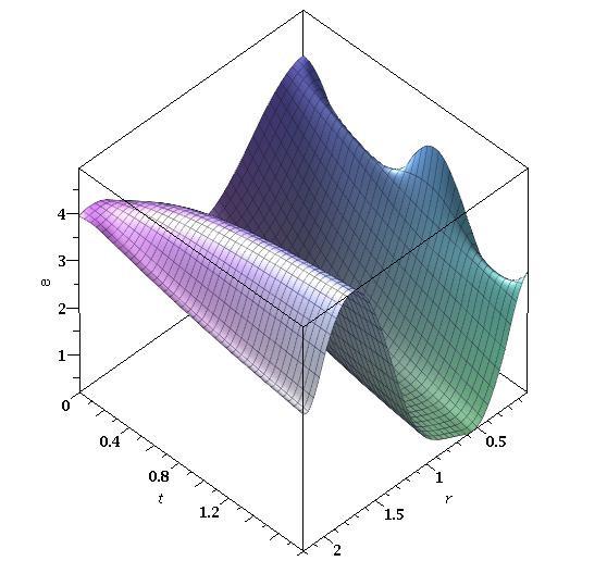
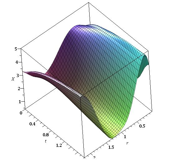
Figure 1: stable solution of $X,\omega$ and $N$ for the case of a constant gauge field. The potential is $V=\beta_{1}X^{\beta_{2}}\omega^{\frac{2}{3}-\frac{\eta\beta_{2}}{y_{0}}}$. We took for the initial values of the scalar and dilaton field a cosine and sine function respectively. For $N$ we took the vacuum solutions of the Appendix A. Further, we applied Neumann boundary conditions. Note that $N$ develops a singularity and approaches to a constant value for increasing time. The solution depends critically on the parameters of the potential, for example, the scale $y_{0}$ of the extra dimension.

2.1.3 The numerical solution

It is clear that we can have breather modes of our scalar-dilaton system. In figure 1 and 2 we plotted a typical solution in the case of a constant gauge field.

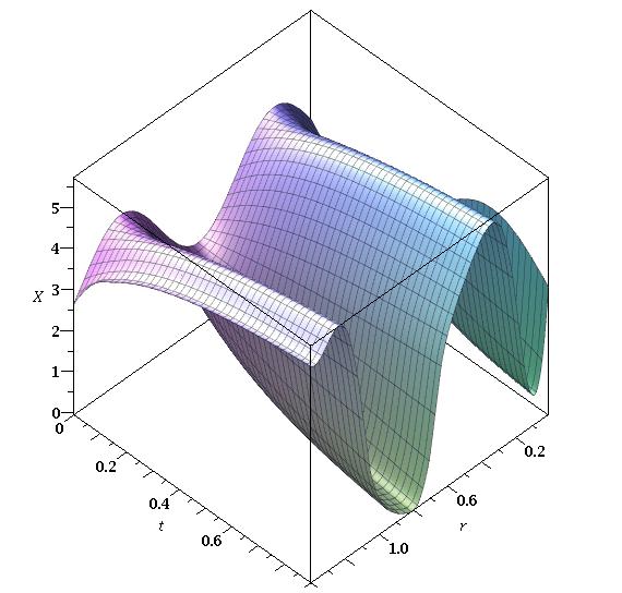
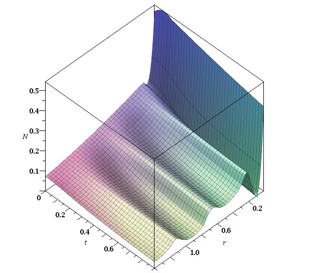
Figure 2: As figure 1, with now as initial value for $\omega$ a $\tanh$ function. We observe that the polynomial behavior in the metric component $N$ is induced by the dilaton. We also plotted the total metric component $\omega^{4}N^{2}$

3 On the double cover of the Klein surface, Riemann surfaces and antipodicity

3.1 Motivation for the Klein surface

For the $S^{2}$ we could apply the stereographic projection $S^{2}\rightarrow\mathds{R}P^{2}\rightarrow\mathds{C}P^{1}$. In order to make the map one-to-one, one applies the $\mathds{Z}_{2}$ symmetry identification: the two antipodal planes are identified, $z\rightarrow-\frac{1}{\bar{z}}$ (see figure 3). In our situation, we uplift the projection to $S^{3}\subset\mathds{R}^{4}$ and use cylindrical coordinates $(r,\varphi)$.

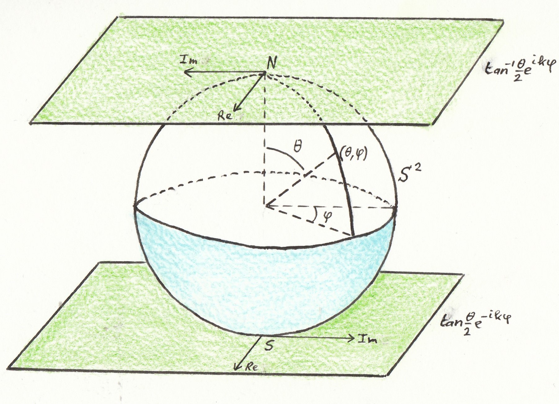
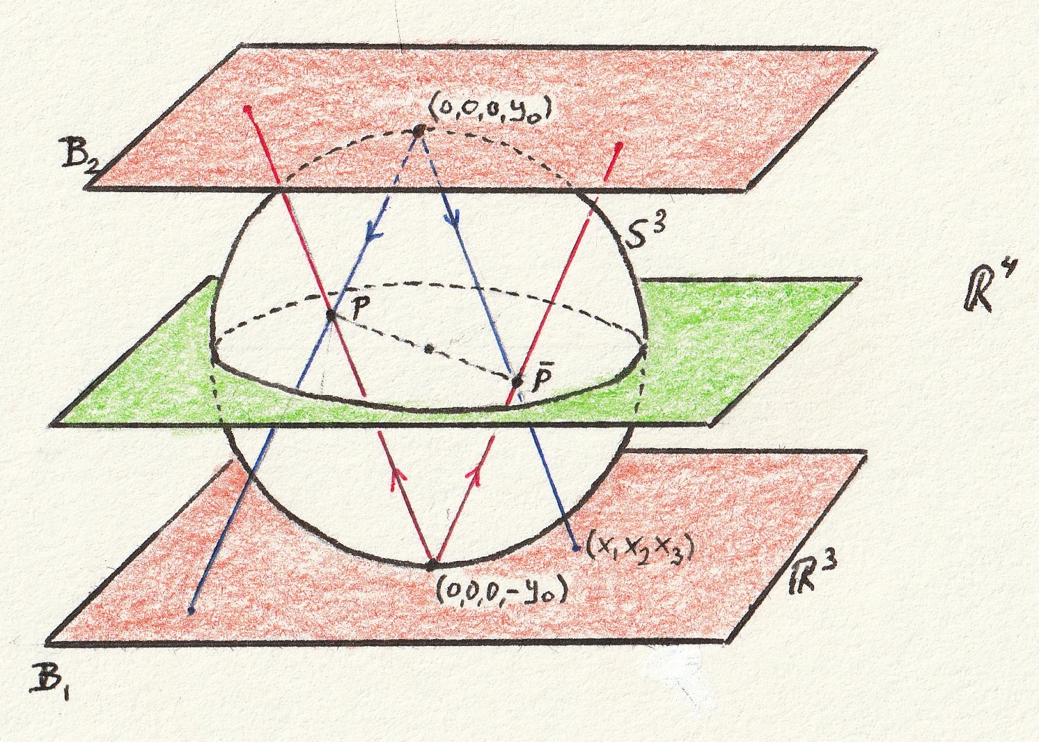
Figure 3: Left: the stereographic projected $S^{2}\rightarrow\mathds{R}P^{2}\rightarrow\mathds{C}P^{1}$. In order to make the map one-to-one, one applies the $\mathds{Z}_{2}$ symmetry identification: the two antipodal planes are identified, $z\rightarrow-\frac{1}{\bar{z}}$. Right: stereographic projection of $S^{3}\subset\mathds{R}^{4}\simeq\mathds{C}\times\mathds{C}$ with also antipodal identification, representing the projection of an embedded Klein bottle.

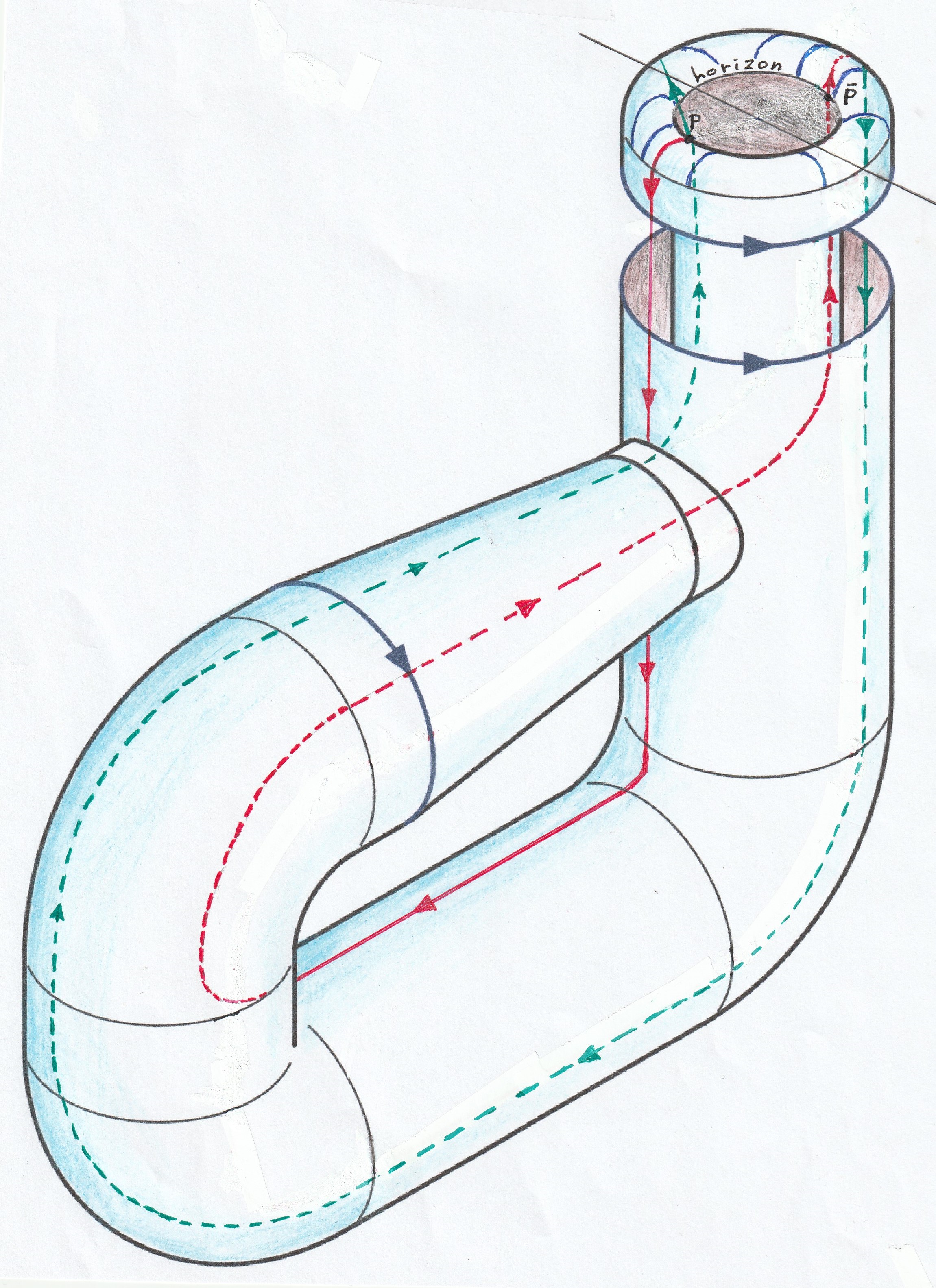
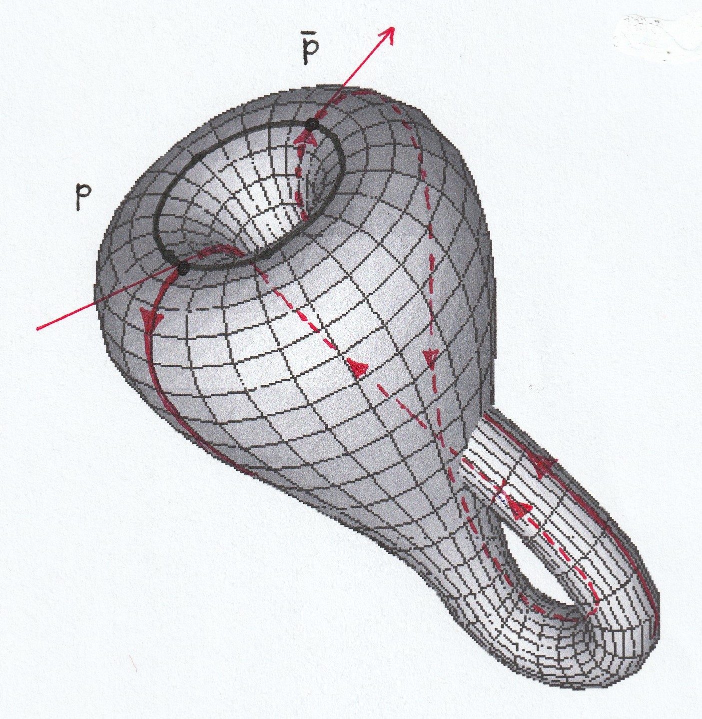
Figure 4: Artist impression of the trajectory of a scalar (Hawking-) particle on the Klein surface. $P$ and $\bar{P}$ are the antipodes. Again, we have a $\mathds{Z}_{2}$ symmetry identification (see figure 3), now for the both sides of the brane: $g_{\mu\nu}({\bf x},\mathpzc{y})=g_{\mu\nu}({\bf x},\mathpzc{-y})$. Note that we apply a slightly different antipodal mapping. We are dealing here with cylindrical symmetric Kerr-like spacetime, where we expand the scalar field in cylindrical harmonics $\Phi_{n,m}=\eta X(r,t)e^{in\varphi}Y_{m}(\Omega)$, in stead of spherical ones. Further, we replace the "cut-and-paste" method by the antipodicity in the bulk space. We can bypass the notion of "quantum clones" proposed by ´t Hooft recentlythooft2022 .

By means of the Hopf fibration, one then makes the connection with real spacetime. For details, we refer to Slagterslagter2022c and Urbantkeur2003 . Another important characteristic of the non-orientable Klein surface is the fact that meromorphic functions remain constantalling1971 . Our solution for $N$ is meromorphic. Further, the Klein surface is homeomorphic to the connected sum of two projective planes.

In the past, intensive research was done on the fundamental group structure of compact surfaces in $m$ dimensions. It is clear that, for example, the torus possesses the structure of two infinite cyclic groups. For the projective plane, the cyclic group of order 2. For the Klein bottle, the fundamental group can be presented by two generators $a,b$ and $baba^{-1}$massey1971 .

We constructed our model in the 5D RS warped spacetime. So the question is how we can imagine the evolution of the Hawking particles created near the horizon, say point $P(U,V,z,\varphi,\mathpzc{y})$ in figure 4. The in-going particle can travel on the Klein surface, in order to leave in the antipode $\bar{P}(-U,-V,-z,\varphi+\pi,-\mathpzc{y})$ the horizon ($J:P\rightarrow\bar{P}$ is an inversion in 5D).

The real physics still takes place on the brane. Effectively, we replaced the "cut-and-past" method in $\mathds{R}^{3}$ by the imaginary transport in $\mathds{R}^{4}$ (via the Hopf fibration of the 3-sphere in $\mathds{R}^{4}$.

We know that complete embedded surfaces in $\mathds{R}^{3}$ must be orientable, otherwise we have self-intersection, so the genus changes. Non-orientable surfaces immersed in $\mathds{R}^{3}$ does not have global Gauss maps, so no well defined mean curvature. So the application of the Klein surface embedded in $\mathds{R}^{4}$ is quite interesting in our context. First, we complexify our hyper-surfaceslagter2022c . Let us write our coordinates $(r,z,\mathpzc{y},\varphi^{*})$ as

$${\cal V}=z+i\mathpzc{y}=Re^{i\varphi_{1}},\qquad{\cal W}=x+iy=re^{i\varphi_{2}},$$ (42)

where the antipodal map is now ${\cal V}\rightarrow-{\cal V}\equiv-R^{2}/\bar{\cal V},{\cal W}\rightarrow-{\cal W}\equiv-r^{2}/\bar{\cal W}$. Further, ${\cal V}\bar{\cal V}=z^{2}+\mathpzc{y}^{2}=R^{2},{\cal W}\bar{\cal W}=x^{2}+y^{2}=r^{2}$. And after inversion

$$z=\frac{1}{2}({\cal V}+\bar{\cal V}),\qquad\mathpzc{y}=\frac{1}{2i}({\cal V}-\bar{\cal V}),\hskip 14.22636pt$$ (43)

$$x=\frac{1}{2}({\cal W}+\bar{\cal W}),\qquad y=\frac{1}{2i}(({\cal W}-\bar{\cal W}),$$ (44)

$$\varphi_{1}=i\log\sqrt{\frac{\bar{\cal W}}{{\cal W}}}\quad\varphi_{2}=i\log\sqrt{\frac{\bar{\cal V}}{{\cal V}}}.$$ (45)

We can write

$$dz^{2}+d\mathpzc{y}^{2}+dx^{2}+dy^{2}=d{\cal V}d\bar{\cal V}+d{\cal W}d\bar{\cal W}.$$ (46)

We now have $|{\cal V}|^{2}+|{\cal W}|^{2}=x^{2}+y^{2}+z^{2}+\mathpzc{y}^{2}=r^{2}+R^{2}$. We identified $\mathds{C}^{1}\times\mathds{C}^{1}$ with $\mathds{R}^{4}$ and so contains $S^{3}$, given by $|{\cal V}|^{2}+|{\cal W}|^{2}=const.$ Every line through the origin, represented by $({\cal V},{\cal W})$ intersects the sphere $S^{3}$, for example $(\lambda{\cal V},{\lambda\cal W})$ with $\lambda=\frac{1}{\sqrt{|{\cal V}|^{2}+|{\cal W}|^{2}}}$. Thus the homogeneous coordinates can be restricted to $|{\cal V}|^{2}+|{\cal W}|^{2}=1.$ The point $({\cal V},{\cal W})\in S^{3}\subset\mathds{C}^{1}\times\mathds{C}^{1}$ with $|{\cal V}|^{2}+|{\cal W}|^{2}=1$, becomes by the complexification, a point of $S^{2}$, so with the single complex coordinate ${\cal Z}=\frac{{\cal V}}{{\cal W}}$. We have now a map $H:S^{3}\rightarrow S^{2}$, which is continuous. One calls this a Hopf map. For each point of $S^{2}$, the coordinate $({\cal V},{\cal W})$ is non unique, because it can be replaced by $(\lambda{\cal V},\lambda{\cal W})$, such that $|\lambda|^{2}=1,\lambda\in S^{1}$. SWe will now write $\mathds{C}_{1}$ for $S^{2}/\{\infty\}$ and $\mathds{C}_{2}$ for $S^{2}/\{0\}$ and admitting coordinates ${\cal Z}$ and ${\cal Z}^{\prime}=\frac{1}{{\cal Z}}$ respectively.

If we write

$${\bf H}=\begin{pmatrix}z+i\mathpzc{y}&x+iy\\ -x+iy&z-i\mathpzc{y}\end{pmatrix}=\begin{pmatrix}\cal{V}&\cal{W}\\ -\cal{\bar{W}}&\cal{\bar{V}}\end{pmatrix}$$ (47)

with $det({\bf H})=|{\cal V}|^{2}+|{\cal W}|^{2}$ and $\mathds{R}^{4}\cong{\bf H}$, we can describe the mapping also with normalized quaternions $\mathds{A}=[a,{\bf A}]=[\cos\alpha,\sin\alpha{\bf n}]$ as binary rotationsaltman1986 . This is clarifying, when we consider the covariance covering groups, such as the $SO(3)$ and $SU(2)$. A rotation is actually represented by two antipodal points on the sphere (a kind of double cover) as a point on the hypersphere in 4D. Each rotation represented as a point on the hypersphere is matched by its antipode on that hypersphere. The quaternion represents a point in 4D. Constrained to unit magnitude, yields then a 3D space, i.e., the surface of a hypersphere. The group of unit quaternions $S^{3}\subset{\bf H}$ is isomorphic with $SU(2)$. We identify $S^{3}$ and $SU(2)$ with the isomorphism. The relation with the Möbius group $G$ is then easily made (see Tothtoth2002 or Slagterslagter2022c ) and so with the alternating group ${\cal A}_{5}$, isomorphic with the binary symmetry group of the icosahedron (see for exampletoth2002 ). Because the icosahedron can be circumscribed by 5 tetrahedra, they form an orbit of order 5 symmetry rotations of the icosahedron. These symmetries are subgroups of the icosahedron symmetry group. The connection with our quintic solution was made in a former studyslagter2022c , by the observation that the vertices of the icosahedron, stereographically projected to $\mathds{C}$, are

$$0,\infty,\gamma^{j}(\gamma+\gamma^{4}),\gamma^{j}(\gamma^{2}+\gamma^{3}),\quad j=0,..4,\quad\gamma=e^{\frac{2\pi i}{5}}.$$ (48)

Shortly stated, for the icosahedral Möbius group, by suitable orientation of the axes, we can write the linear fractional transformations as $\zeta\rightarrow\gamma^{m}\zeta(m=0..4)$. The binary icosahedral group $G^{*}$ associated with the Möbius group $G\subset{\cal M}_{0}(\mathds{C})$.

Let us now try to make the connection with state vectors in $\mathds{C}^{2}$. On a complex Hilbert space ${\cal H}$, taken as the space $\mathds{C}^{2}$ of pairs $\lvert{\cal U}\rangle=({\cal V},{\cal W})$ and equipped with scalar product, one can define a state vector by the set of multiples $\lambda\lvert{\cal U}\rangle$, with $|\lambda|=1$ and normalization condition $\langle{\cal U}|{\cal U}\rangle=1$. Further, we have the matrix

$$\rho:=\lvert{\cal U}\rangle\langle{\cal U}\rvert,\quad\rho_{ij}=\begin{pmatrix}\cal{V}\cal{\bar{V}}&\cal{V}\cal{\bar{W}}\\ \cal{W}\cal{\bar{V}}&\cal{W}\cal{\bar{W}}\end{pmatrix},$$ (49)

with $\rho^{\dagger}=\rho$ and ${\bf Tr}(\rho)=1$. We define now the vector $\vec{{\bf V}}=(V_{1},V_{2},V_{3})\in\mathds{R}^{3}$, with $\rho_{11}=\frac{1}{2}(1-V_{3}),\rho_{22}=\frac{1}{2}(1-V_{3})$ and $\rho_{21}=\bar{\rho}_{12}=\frac{1}{2}(V_{1}+iV_{2})$. We can write $\rho=\frac{1}{2}(\mathds{I}+\vec{{\bf V}}.{\bf\sigma})$, with $\sigma$ the Pauli matrices. Furter, $1-{\bf V}^{2}\geq 0$. We define the vector $\vec{{\bf X}}=(x,y,z,\mathpzc{y})$ and take $\lambda=e^{i\alpha}$ a phase factor. We then write ${\cal W}_{i}\rightarrow e^{i\alpha}{\cal W}_{i},{\cal V}_{i}\rightarrow e^{i\alpha}{\cal V}_{i}$. So $\vec{{\bf X}}\rightarrow\cos(\alpha)\vec{{\bf X}}+\sin(\alpha)J\vec{{\bf X}}$, with $J\vec{{\bf X}}=(-X_{2},X_{1},-X_{4},X_{3})=(-y,x,-\mathpzc{y},z)$ a normalized combination of two orthogonal unit vectors of $\mathds{R}^{4}$ for all $\alpha$. In fact, we obtain a Hopf fibration of $S^{3}$. This fibering is the stereographic projection on $X_{4}=\mathpzc{y}=0$ of $S^{3}$, an analogy of the stereographic projection of one dimension lower. See figure 3. Remember, we identified the antipodal points, so we obtain a Klein bottle $\mathds{K}=\{({\cal V},{\cal W})\mathchar 24635\relax\;|{\cal V}|^{2}-|{\cal W}|^{2}=\cos(\theta)\}\in S^{3}\subset\mathds{C}^{2}$ in $\mathds{R}^{3}$ (see Eq.(51)). However, it is embedded in our $\mathds{R}^{4}$. If we project from $(0,0,0,\pm\mathpzc{y}_{0})$, the running point $\vec{{\bf X}}$ on $S^{3}$ is now related to its stereographic image $\vec{{\bf x}}=(x_{1},x_{2},x_{3})$ by $X_{4}=\pm\frac{{\bf x}^{2}-1}{{\bf x}^{2}+1}$, $X_{i}=\frac{2x_{i}}{{\bf x}^{2}+1}$. For normalization of $\lvert{\cal Z}\rangle$, we first define $\varphi=\varphi_{2}-\varphi_{1}$ and write

$${\cal W}=\cos(\frac{\theta}{2})e^{i\varphi_{1}}=\cos(\frac{\theta}{2})e^{-i\varphi/2}e^{i(\varphi_{1}+\varphi_{2})/2}$$ (50)

$${\cal V}=\sin(\frac{\theta}{2})e^{i\varphi_{2}}=\sin(\frac{\theta}{2})e^{i\varphi/2}e^{i(\varphi_{1}+\varphi_{2})/2}.$$ (51)

Varying $\alpha$ will only change $(\varphi_{1}+\varphi_{2})/2$ and not $\varphi$ and $\theta$. Further we have $V_{3}=\cos(\theta)$ and $V_{1}+iV_{2}=\sin(\theta)e^{i\varphi}$, ${\cal Z}=\frac{{\cal V}}{{\cal W}}=\tan(\theta/2)e^{i\varphi}$, with the antipodal identification $\varphi\rightarrow\varphi+\pi$.

One can compare this visualization by the orientable counterpart situation of the torus. For details, see Tothtoth2002 (section 1.4) or Urbantkeur1990

So if we consider a Hawking particle falling in, it travels for a while in $\mathds{R}^{4}$ from $\mathpzc{y}_{0}\rightarrow-\mathpzc{y}_{0}$ arriving at the antipodal point in $\mathds{R}^{3}$.

3.2 The elapse time in the bulk

One could wonder if one can estimate the elapse propertime of a particle when it moves in the bulk space and back to the brane. Our horizon $r_{H}$ is determined by $a_{i}$ (see Eq.(95)). We assume that $y_{0}\sim 10^{-5}m$maartens2010 and let us take $r_{H}\sim 10^{7}$m. See, for example, Maldacenamaldacena2021 . The proper traversal time, $t_{e}$, of the Klein surface will be of the order of $r_{H}$. Further, the trajectory on the Klein surface in the bulk, $l_{b}$, will be of the order $\frac{t}{t_{e}}$, with $t$ the asymptotic time and $t_{e}$ the proper time. If we adapt the approximation of the wormhole model on the RS spacetime of Maldacena, we could obtain an elapse time of the order $10^{-2}$ s, while $t$ would be must larger.

It would be of interest if one could measure this elapse time in the Hawking radiation. One could obtain an estimate of $y_{0}$.

3.3 The scalar equation on the single-sided black hole

It is obvious that strong gravitation interactions will take place near the horizon. The scattering process by in- and out-going wave functions can be handled by different approximations. One can make a distinction between the near horizon behavior and the further away approximation by means of the Regge-Wheeler potentialbetzios2021 . An effective gravitational potential for the propagating modes on a Schwarzschild background then enters the Klein-Gordon equation.

We will consider here the antipodal boundary condition of the single-sided black hole. This idea was already studied by Schrödingerschrod1957 . It was used by Gibbonsgib1986 in connection with CPT invariance and quantum mechanics on the identified space. The method was also used by Sanchez, et al.san1987 in connection with the quantum Fock space. We applied the mapping on the RS spacetimeslagter2022c . We already observed that the scale of the extra dimension $y_{0}$ entered the effective 4D field equations. Further, the dynamical evolution of the 4D Einstein equations were modified by the projection of the 5D Weyl tensor on the brane and carried the information of the gravitation field outside the brane (the so-called "Kaluza-Klein"modes).

We will use the expansion of the scalar field in cylindrical harmonics

$$\Phi_{n,m}=\eta X(r,t)e^{in\varphi}{\bf Y}_{m},$$ (52)

where $X(r,t)$ fulfills the PDE’s of section 2. Further, we have $e^{in(\varphi+\pi)}=(-1)^{n}e^{in\varphi}$. For ${\bf Y}_{m}$ we can choose

$${\bf Y}_{m}=\sum_{m}\Bigl{(}A_{m}\cos(m\varphi)+B_{m}\sin(m\varphi)\Bigr{)}.$$ (53)

We can in this way always obtain a factor $(-1)^{(n+m)}$ in front of the right-hand side in Eq.(52). Further, the field equations are invariant under $t\rightarrow-t$ (see 4.2 and the Appendix A). Note that for antipodicity, we need the map: $e^{i\varphi}\rightarrow e^{i(\varphi+\pi)}$.

The reader must remind himself that in our conformal model, the scale is determined by the dilaton $\omega$. In the vacuum situation (see Appendix A) an exact time-dependent solution was found. Now we conjecture that in the non-vacuum situation, more information can be gathered by our model about the scattering process when approaching smaller scales. The distinction one usually makes between the near horizon region and the Regge-Wheeler region, can be replaced by the dynamical interaction of the scalar waves and the dilaton field. The distinction was necessary because gravity comes into play. Further, the small scale behavior translates itself in the dilaton and the conformally flat $\tilde{g}_{\mu\nu}$. Remember now that the dilaton field (part of the gravitation metric) describes the complementarity between the local and outside observer and can be used (by $\Omega$, see Eq.(3)) to define the vacuum state the local observer experiences (see section 2.1). It is conjectured (also from the numerical solutions) that the spacetime becomes singular-free when $t\rightarrow\infty$, except for $r=0$, which is no problem because there is no inside of the Klein surface.

3.4 Comparison with AdS

The elliptic interpretation was historically first studied in cosmology, i.e., in the deSitter spacetime. Let us consider the inversion in $\mathds{R}^{5},J:{\bf X}^{a}\rightarrow-{\bf X}^{a},(a=1...5)$, and the hypersurface $\frac{1}{H^{2}}=-t^{2}+x^{2}+y^{2}+z^{2}+\mathpzc{y}^{2}$, which is the deSitter spacetime in a 5D spacetime

$$ds^{2}=-dt^{2}+dx^{2}+dy^{2}+dz^{2}+d\mathpzc{y}^{2},$$ (54)

with $H^{-1}$ the radius of the hypersphere and $t$ the proper time along a set of geodesics. The symmetries of this pseudo sphere is the 10 parameter Poincaré group in Minkowski spacetime. One writes the pseude sphere ($\eta=-H^{-1}exp(-Ht)$)

$$ds_{dS}^{2}=-dt^{2}+e^{2Ht}(dx^{2}+dy^{2}+dz^{2})=\frac{1}{H^{2}\eta^{2}}(-d\eta^{2}+dx^{2}+dy^{2}+dz^{2}).$$ (55)

The group invariance of the deSitter spacetime can now be used to apply a high-frequency behavior of the scalar field in order to define the prefered vacuum state as measured by the observers on the geodesics. From the scalar equation (like Eq.(14)), one easily find

$$\partial_{t}^{2}\phi+3H\partial_{t}\phi-e^{-2Ht}\sum_{i}\partial_{i}^{2}\phi+M^{2}\phi=0,$$ (56)

with $M^{2}=m^{2}+12\xi H^{2}$. We expand the field operator $\phi$ now as

$$\phi=\sum_{k}\Bigl{\{}A_{\vec{k}}f_{\vec{k}}(x)+A^{\dagger}_{\vec{k}}f^{*}_{\vec{k}}(x)\Bigr{\}},\quad f_{\vec{k}}=\frac{1}{\sqrt{2Ve^{3Ht}}}2^{i\vec{k}.\vec{x}}h_{k},$$ (57)

with $k^{i}=2\pi n^{i}/L,n^{i}$ an integer, $k=|\vec{k}|$ and $L$ the dimension of the 3-space ($V\sim L^{3}$). The term $Ve^{3Ht}$ represents here the physical volume of the cube on which one applies the periodic boundary conditions. Further $h_{k}$ satisfies a Bessel equation

$$v^{2}\frac{d^{2}}{dv^{2}}h_{k}+v\frac{d}{dv}{h_{k}}+(v^{2}-\nu^{2})h_{k}=0,\quad\nu=\sqrt{\frac{9}{4}-\frac{M^{2}}{H^{2}}},\quad v=\frac{ke^{-Ht}}{H}.$$ (58)

One can also use $u\equiv-v$ as independent variable. $v$ is the ratio of the momentum of a particle to the expansion $H$. In this context, an observer on a geodesic in the deSitter spacetime will be surrounded by isotropic thermal radiation ( with wavelength $\lambda$) coming from de geodesic’s Hubble horizon with temperature $T_{H}=H/(2\pi k_{B})$. So $v$ represents also the ratio of the proper radius $H^{-1}$ to $\lambda/(2\pi)$. For small wavelength, compared with the radius of curvature and slowly changing of $a(t)=e^{Ht}$, we assume that the positive frequency solutions $f_{\vec{k}}$ possesses an adiabatic form, i.e., the WKB-solution. We can write

$$f_{\vec{k}}({\bf x})=\frac{1}{\sqrt{2Va^{3}\omega_{k}}}e^{i(\vec{k}.\vec{x}-\int\omega_{k}dt)},\quad\omega=k/a(t).$$ (59)

Further, $h_{k}$ has the asymptotic form

$$h_{k}\sim\frac{1}{\sqrt{\omega}}e^{-i\int\omega_{k}dt}.$$ (60)

For large $k,h_{k}\sim\frac{1}{\sqrt{Hv}}e^{iv}$. The general solution of the Bessel equation, Eq.(58), is

$$h_{k}=\sqrt{\frac{\pi}{2H}}\Bigl{\{}E(k)H_{\nu}^{(2)}(v)+F(k)H_{\nu}^{(1)}(v)\Bigr{\}},$$ (61)

with $H_{\nu}$ Hankel functions. When $k\rightarrow\infty$, we have $E(k)\sim 0,F(k)\sim 1$. From the deSitter symmetries, one finally obtains the creation and annihilation operators

$$f_{\vec{k}}=\sqrt{\frac{\pi}{4HV}}e^{-3/2Ht}H_{\nu}^{(1)}(k\frac{k}{H}e^{-HT})e^{i\vec{k}.\vec{x}},$$ (62)

and hence the vacuum state. For $\xi=1/6$ and $m=0$, we obtain $H_{\frac{1}{2}}^{(1)}=-i\sqrt{\frac{2}{\pi v}}e^{iv}$. For $u=-v,H_{\nu}^{(1)}(v)$ is replaced by $H_{\nu}^{(2)}(u)$. Note that in calculating the expectation values such as $<\phi(\vec{x},t)^{2}>$, there appears infrared or ultra violet singularities in this two point function, at least for $\xi=0$.

In the antipodal situation of the deSitter spacetime, the expectation value becomes (symmetric and antisymmetric)fol1987

$$<\phi_{JA/S}(\vec{x},t)^{2}>=<\phi(\vec{x},t)^{2}>\pm<\bar{\phi}(\vec{x},t)^{2}>,$$ (63)

with

$$<\bar{\phi}(\vec{x},t)^{2}>=\frac{1}{16\pi\cos(\pi\nu)}\{m^{2}+12(\xi-1/6)H^{2}\}.$$ (64)

What remains is the problem with the Fock vacuum. This is essential, because one can always add an antipodal source (see discussion by Gibbonsgib1986 ).

We now return to our situation. In the next sections we investigate some topological aspects.

4 Topological aspects: relation with the instanton and minimal embedding in $\mathds{K}$

4.1 Some history

It is well known that on Minkowski spacetime $\mathds{R}^{d+1}$, the action of the static Yang-Mills-Higgs configuration $({\bf A},\Phi)$ equals the Euclidean action on $\mathds{R}^{d}$. The field equations of the Euclidean action, for example, in $\mathds{R}^{4}$ in this model, allow soliton solutions, which are so time-independent finite energy solutions to the variational equations for the action density on the $\mathds{R}^{5}$ Minkowski spacetime. For the $d=4$ pure Yang-Mills case, they are called instantons. It turns out that their "curvatures" are self-dual.

In the "transcendental" book of Jaffe and Taubesjaf1981 one finds a nice introduction of these issues. We can now make the connection with our model.

4.2 Connection with the warped spacetime solution

Let us write our (4+1) dimensional spacetime on the 5 dimensional Riemannian manifold:

$$ds^{2}=\omega(\tau,r,y)^{4/3}\Bigl{[}N(\tau,r)^{2}d\tau^{2}+\frac{1}{N(\tau,r)^{2}}dr^{2}+dz^{2}+r^{2}(d\varphi+N^{\varphi}(\tau,r)d\tau)^{2}+d\mathpzc{y}^{2}\Bigr{]}.$$ (65)

One easily obtains the field equations in $d$ ($d=4,5$; compare with Eq.(90) and Eq.(92) in the pseudo-Riemannian spacetime)

$$\ddot{\omega}=N^{4}\omega^{\prime\prime}-\frac{d}{\omega(d-2)}(N^{4}\omega^{\prime 2}-\dot{\omega}^{2}),$$ (66)

$$\ddot{N}=\frac{3\dot{N}^{2}}{N}+N^{4}(N^{\prime\prime}+\frac{3N^{\prime}}{r}+\frac{N^{\prime 2}}{N})$$ (67)

$$+\frac{(d-1)}{(d-3)\omega}\Bigl{[}N^{5}\Bigl{(}\omega^{\prime\prime}+\frac{\omega^{\prime}}{r}+\frac{d}{2-d}\frac{\omega^{\prime 2}}{\omega}\Bigr{)}+N^{4}(\omega^{\prime}N^{\prime}-\dot{\omega}\dot{N}\Bigr{]},$$ (68)

with the dot representing now $\partial_{\tau}$. Note that we are dealing here now with hyperbolic PDE’s in stead of elliptic ones.

The exact solution is again given by the solution of Eq.(93) and Eq.(95) (in the pseudo-Riemannian spacetime). We repeat that our original pseudo-Riemannian 5D spacetime delivers an effective 4D Riemannian spacetime on the brane

$$ds^{2}=\frac{N_{1}^{2}}{N_{2}^{2}}(dt^{*2}+dr^{*2})+dz^{2}+r^{2}d\varphi^{*2},$$ (69)

where $r$ can be expressed in $r^{*}$ (Appendix B). The topology is $\mathds{R}^{2}_{+}\times\mathds{R}^{1}\times S^{1}$. The $\varphi^{*}$ causes no problems, because the $N^{\varphi}$ component decouples from the equations for $N$ and $\omega$. $\mathds{R}^{2}_{+}$ is still conformally flat.

It is legitimate to conjecture that in the non-vacuum case, the scalar field will also be the same on the Riemannian spacetime. This could be used in order to solve the issue of construction of the quantum wave functions as elements of the Fock space. One of the entangled particles travels on the Klein surface on the hypersurface embedded in the 5D spacetime and remains a pure state. In the next sections, we will enlighten this issue.

4.3 Some other aspects of the Klein bottle

In our model, we need the Klein surface $\mathds{K}$, the compact sum of two projective planes. Our conjecture is, that our solution can be seen as a dynamical solution embedded in our $(4+1)$ spacetime. More precisely, if ${\cal N}$ is the sub manifold with metric $g$, i.e., the metric on our effective 4D spacetime, then ${\cal N}$ is diffeomorphic to the hyperbolic 5D spacetime: $\chi:\mathds{R}^{5}\rightarrow{\cal N}$. The Riemannian manifold $({\cal N},g)$ must be conformally flat, which is the case here.

Now physicists are interested in the topology of moduli spaces of self-dual connections on vector bundles over Riemannian manifolds. One reason was that on these spaces the instanton approximation to the Green functions of Euclidean quantum gravity Yang-Mills theory can be expressed in terms of integrals over moduli spaces. One needs then the metric and volume form of the moduli spaces.

From the investigations of Groisser, et.al,gross1987 , we conjecture that we can consider $\mathds{K}$ as a 4-sphere in our hyperbolic pseudo Riemannian spacetime. This suspicion is fueled by the solution of section 4.2, and the work on the orientable counterpart model of Groisser (and references therein).

More precisely, on a Riemannian 5-manifold, one can proof that there exists a coordinate diffeomorphism $\xi:\mathds{R}^{5}\rightarrow{\cal N}$ for which the pullback of the metric $\mathpzc{g}$ on ${\cal N}$ is given by $(\xi^{*}\mathpzc{g})_{ij}=\Psi^{2}({\bf x})\delta_{ij}$. Further, the Riemannian manifold $({\cal N},\mathpzc{g})$ is conformally flat with finite radius and volume. The action of $SO(5)$ on $S^{4}$ induces an isometry on ${\cal N}$ whose pullback, via $\xi$, is the usual action $SO(5)$ action on $\mathds{R}^{5}$. So ${\cal N}$ can isometrically included as the interior of a compact Riemannian manifold with boundary, say $\bar{\cal N}$, whose boundary $\partial\bar{\cal N}$ is isometric to the 4-sphere of constant radius. The embedding $\partial\bar{\cal N}\rightarrow{\cal N}$ is totally geodesic. The sphere $\partial\bar{\cal N}$ is conformally equivalent to the original manifold $(S^{4},\mathpzc{g})$ and points on $\partial\bar{\cal N}$ corresponds to instantons which are concentrated at a single point on $S^{4}$. It is remarkable that the $\Phi({\bf x})$ is determined by a PDE which is comparable with our scalar equation (${\cal N}$ has no constant curvature).

A remark must be made about the $\mathds{Z}_{2}$ symmetry in the original description of the antipodal mappingthooft2021 . At the border of region I and II in the Penrose diagram, the antipodes on a 3-sphere were glued together and the transverse $(\theta,\varphi)$ part is a projected 2-sphere. In our model, it is replaced by the projected 3-sphere $(z,\varphi,\mathpzc{y})$ using the $\mathds{Z}_{2}$ symmetry of the bulk space $(U,V,z,\varphi,\mathpzc{y})$. No cut and past procedure is necessary.

However, a lot of unsolved issues need to be attacked. In particular, the firewall transformation description in the warped spacetime.

5 Notes on the information paradox

There are some known facts about the information paradox. An outside observer will register the Hawking radiation as thermal, i.e., in a mixed state, while a local observer is in doubt about the vacuum state. Further, the evolution of the wave function of the in-falling particle must be unitary, i.e., it satisfy the Schrödinger equation $\lvert\chi(t_{1})\rangle=U(t_{1},t_{2})\lvert\chi(t_{2})\rangle$ and is bijective. It is believed that during black hole evaporation, information of the quantum state is preserved. Information loss is inconsistent with unitarity. So the problem is how to handle the controversy between the pure quantum state of the in-falling particles and the mixed state property of the Hawking radiation.

In our model we do not rely on replica wormholes, but instead on the warped spacetime and Klein surface.

By the antipodal mapping in $\mathds{R}^{4}$, we have also $e^{in\varphi}\rightarrow e^{in(\varphi+\pi)}$. This can be "visualized" by considering in figure 3 (right) points on the circle on $S^{3}$ (for example $\alpha\sim e^{in\varphi}$) for which

$$\sin(\theta/2)e^{in\varphi}{\cal V}(\alpha)-\cos(\theta/2){\cal W}(\alpha)=0.$$ (70)

From the real part, we obtain the plane after the stereographic projection,

$$x_{3}=\tan(\theta/2)(\cos(\varphi)x_{1}-\sin(\varphi)x_{2}.$$ (71)

If we apply $e^{in\varphi}\rightarrow e^{in(\varphi+\pi)}$, the plane is rotated over $\pi$. The imaginary part delivers the two spheres ${\bf x}^{2}\mp\tan(\theta/2)(\sin(\varphi)x_{1}+\cos(\varphi)x_{2})=1$.

We found in section 3 that the in-falling Hawking particle travels for a while on the Klein surface in $\mathds{R}^{4}$. Now consider the state

$$\lvert\chi\rangle=\lvert\hat{\chi}\rangle e^{in\varphi}$$ (72)

and the density matrix

$$\rho_{A}=\sum_{i}p_{i}\lvert\chi_{i}\rangle_{A}{{}_{A}}{\langle\chi_{i}\rvert}$$ (73)

as mixture of pure states and weights $p_{i}$ with $\sum p_{i}=1$. Further,${\bf Tr}\rho_{A}=1$ and $\rho_{A}^{2}=\rho_{A}$. The density matrix doesn’t contain the phase. So the change of the azimuthal angle $\varphi$ has no influence on the pure states. This can be compared with the the "pureness" of $\rho$ in Eq(49) of normalized state vectors on $S^{2}\subset\mathds{R}^{3}$. In addition to $\vec{{\bf V}}$

$$\vec{{\bf V}}=\Bigl{(}{\cal V}{\cal\bar{W}}+{\cal W}{\cal\bar{V}},i({\cal V}{\cal\bar{W}}-{\cal W}{\cal\bar{V}}),|{\cal V}|^{2}-|{\cal W}|^{2}\Bigr{)},$$ (74)

independent of a phase change in $\lvert{\cal U}\rangle=({\cal V},{\cal W})$, we define

$$\vec{{\bf Z}}=\vec{{\bf P}}+i\vec{{\bf Q}}=\Bigl{(}{\cal V}^{2}-{\cal W}^{2},i({\cal V}^{2}+{\cal W}^{2}),-2{\cal V}{\cal W}\Bigr{)}.$$ (75)

$(\vec{{\bf V}},\vec{{\bf P}},\vec{{\bf Q}})$ form a positively oriented orthonormal triad. Now $\vec{{\bf P}}$ is a unit tangent vector to $S^{2}$ at $\vec{{\bf V}}$. If $\lvert{\cal U}\rangle\rightarrow e^{i\alpha}\lvert{\cal U}\rangle$, then $\vec{{\bf V}}$ is independent of this phase change, while $\vec{{\bf Z}}\rightarrow e^{2i\alpha}\vec{{\bf Z}}$. One can verify that $\vec{{\bf P}}$ registers phase change $mod(\pi)$ only. When $\lvert{\cal U}\rangle\rightarrow-\lvert{\cal U}\rangle$, $\vec{{\bf U}}$ still delivers the same $\vec{{\bf P}}$, while $(\vec{{\bf R}},\vec{{\bf P}})$ determine $\lvert{\cal U}\rangle$ up to sign. Let us now interpret $|\langle{\cal U}|{\cal U^{\prime}}\rangle|^{2}$ (independent of the phase) as a "probability". In language of the geometric picture here, $\sqrt{1-|\langle{\cal U}|{\cal U^{\prime}}\rangle|}=\frac{1}{2}|\vec{{\bf V}}-\vec{{\cal{\bf V^{\prime}}}}|$ represents the diameter of $S^{2}$.

This "visualization"is in fact a Hopf fibration of $S^{3}$ (see also section 3.1) In our case, we are dealing with a time depended situation and state vectors follow the Schrödinger equation

$$\frac{d}{dt}\lvert{\cal U}\rangle(t)=-\frac{1}{\hbar}H\lvert{\cal U}\rangle(t),$$ (76)

with $H$ a Hermitian matrix, with $H=H_{0}\mathds{I}+\vec{{\bf H}}.{\bf\sigma}$. One finally obtains

$$\frac{d{\vec{{\bf V}}}}{dt}=\vec{{\bf V}}=\frac{2}{\hbar}\vec{{\bf H}}\times\vec{{\bf V}},$$ (77)

the time evolution in $S^{2}$. From Eq.(77) we have $\vec{{\bf V}}.\vec{{\bf V}}=0$, so pure states remain pure.

5.1 Another argument

There is another strong argument for considering the topology of the Klein surface. In short, we blow up the 4-manifold to 5D in order to handle the singularities in the curvature and to apply the antipodal map. One can mathematically formulate the topology of a 4-manifold using self-dual connections over de Riemannian $S^{4}$freed1984 . It depends only upon the conformal class of the Riemannian metric. This self-dual connection can be interpreted by the conformal map: $\mathds{R}^{4}\rightarrow S^{4}/\{0\}$ as a self-dual connection or "instanton".

In our 5D RS model (with a finite number of singularities), we found the metric is determined by $N$ and $\omega$ (see appendix A). The solution for $N$ on the effective 4D spacetime is the same, while the $\omega$ contribution is different. This is solely due to the contribution of ${\cal E}_{\mu\nu}$ (Eq.(8)). If we switch to Riemannian $(t\rightarrow i\tau$, a Wick rotation), the solution is for both $N$ and $\omega$ unaltered. Moreover the $\tilde{g}_{\mu\nu}$ is conformally flat. The embedding of the Klein surface was done using the extra dimension ${\bf\mathpzc{y}}$ and the effective spacetime is conformally flat.

Consider now the ball $B^{4}\subset\mathds{R}^{4}$ with the induced metric $\omega^{4}g_{\mu\nu}$ (Eq.(93)). So the scale is $\omega^{4}$. Then the ball $\frac{r}{2\omega}B^{4}\subset\mathds{R}^{4}$ has a curvature $\leq\frac{const}{|\omega|^{4}}$ We interpret the Riemannian 5D warped spacetime Eq.(65), an open 5-ball, as an instanton on $\mathds{R}^{4}$.

In the pseudo-Riemannian spacetime of Eq.(6), the boundary is the non-orientable Klein surface, which we used for the antipodicity in order to maintain the pure states of the Hawking particles.

The importance of the instanton trick, is the fact that in the Riemannian space (or easier, in Minkowski space) they play a crucial role in calculating path integralsfelsager1998 . It turns out that a static solution in $m$ space dimensions is completely equivalent to an instanton in $m$ space-time dimensions.

6 High-frequency approximation close to the horizon

Our time evolution was governed by the Klein-Gorden-type PDE. Although we found a time dependent exact and numerical solution, one should like to describe the quantum effects more precisely. It is a nice exercise to derive the Schrödinger equation from the Klein-Gordon, using the so-called multiple-scale (or high-frequency (HF)) method (see appendix E).

However, we are dealing here also with the polar angle dependency. One usually deals with separability of the wave function in a $(t,r)$ part and spherical harmonics. In our case, this is not possible without extra assumptions. The HF method can offer a solution for this situation (see, for example, Slagterslagter2022d , section 3.3). In some sense, one can keep track of the back reaction of the emitted Hawking particles. In the appendix E.4, we applied the method for the Vaidya spacetime in Eddington-Finkelstein coordinates

$$ds^{2}=-\Bigl{(}1-\frac{2M(u)}{r}\Bigr{)}du^{2}-2dudr+r^{2}(d\theta^{2}+\sin^{2}\theta d\varphi^{2}),$$ (78)

which is the Schwarzschild spacetime with $u=t-r-2M\log(r/2M-1)$. This spacetime is used to demonstrate the loss of mass by gravitational radiation. From Eq.(166) and Eq.(167) we obtain

$$h_{rr}=h_{r\theta}=h_{r\varphi}=0,\qquad h_{\varphi\varphi}=-\sin^{2}\theta h_{\theta\theta}$$ (79)

$$\ddot{k}_{rr}=0,\qquad\dot{h}_{\theta\theta}=r\partial_{r}\dot{h}_{\theta\theta},\qquad\dot{h}_{\theta\varphi}=r\partial_{r}\dot{h}_{\theta\varphi}.$$ (80)

So one writes

$$h_{\theta\theta}=r\alpha(u,\theta,\varphi,\xi),\quad h_{\theta\varphi}=r\beta(u,\theta,\varphi,\xi),\quad h_{\varphi\varphi}=-r\alpha\sin^{2}\theta.$$ (81)

Further, we have

$$\ddot{k}_{r\theta}=\frac{1}{r}\Bigl{(}2\dot{\alpha}\cot\theta+\partial_{\theta}\dot{\alpha}+\frac{1}{\sin^{2}\theta}\partial_{\varphi}\dot{\beta}\Bigr{)},$$ (82)

$$\ddot{k}_{r\varphi}=\frac{1}{r}\Bigl{(}\dot{\beta}\cot\theta-\partial_{\varphi}\dot{\alpha}+\partial_{\theta}\dot{\beta}\Bigr{)},$$ (83)

$$\frac{dM}{du}=-\frac{\ddot{k}_{\phi\phi}+\sin^{2}\theta\ddot{k}_{\theta\theta}}{4\sin^{2}\theta}-\frac{1}{2}r\dot{h}_{uu}-\frac{1}{4}\Bigl{(}\dot{\alpha}^{2}+\frac{\dot{\beta}^{2}}{\sin^{2}\theta}\Bigr{)}+\frac{1}{4}\Bigl{(}\ddot{\alpha^{2}}+\frac{\ddot{\beta^{2}}}{\sin^{2}\theta}\Bigr{)}.$$ (84)

Not all the components of $h_{\mu\nu}$ and $k_{\mu\nu}$ are physical, so one needs some extra gauge conditions. Suitable choice of $\alpha$ and $\beta$ (Choquet-Bruhat uses, for example, $\alpha=0,\beta=g(u)h(\xi)\sin\theta$), leads to a solution to second order which is in general not axially symmetric. We can integrate these zero order equations with respect to $\xi$. One obtains then some conditions on the background fields, because terms like $\int\dot{\alpha}d\xi$ disappear. From Eq.(84), we obtain

$$\frac{dM}{du}=-\frac{1}{4\tau}\int_{0}^{\tau}\Bigl{(}\dot{\alpha}^{2}+\frac{\dot{\beta}^{2}}{\sin^{2}\theta}\Bigr{)}d\xi,$$ (85)

which is the back-reaction of the high-frequency disturbances on the mass $M$. $\tau$ is the period of $\dot{h}_{\mu\nu}$. This expression can be substituted back into Eq.(84). However, in the non-vacuum case, the right-hand side will also contain contributions from the matter fields. In order to obtain propagation equations for $h_{\mu\nu}$ and $k_{\mu\nu}$, one proceeds with the next order equation $R_{\mu\nu}^{(1)}=0$. First of all, Eq.(82), (83) are consistent with $R_{r\varphi}^{(1)}=0$ and $R_{r\theta}^{(1)}=0$. Further, one obtains propagation equations for $\alpha$ and $\beta$ and for some second order perturbations, such as $k_{\varphi\varphi}$. Moreover, the $(\varphi,\theta)$-dependent part of the PDE’s for $\alpha$ and $\beta$ (say $A(\theta,\varphi),B(\theta,\varphi)$) can be separated (for the case $k_{\theta\varphi}\neq 0$):

$$\partial_{\varphi}B+2\sin\theta\cos\theta A+\sin^{2}\theta\partial_{\theta}A=0,$$ (86)

$$\sin^{2}\theta\partial_{\theta\theta}A+7\sin\theta\cos\theta\partial_{\theta}A+4\cot\theta\partial_{\varphi}B+2(5\cos^{2}\theta-1)A+2\partial_{\theta\varphi}B=0.$$ (87)

A non-trivial simple solution is

$$A=\frac{\cos\theta(sin\varphi+\cos\varphi)}{sin^{3}\theta},\quad B=\frac{\sin\varphi-\cos\varphi}{\sin^{2}\theta}+G(\theta),$$ (88)

with $G(\theta)$ arbitrary. So the breaking of the spherically and axial symmetry is evident.

7 Conclusion

On a warped 5D Randall-Sundrum Kerr-like black hole spacetime, we investigated the time evolution of the scalar-gauge field in the conformal invariant gravity model. We analyzed the dilaton-Higgs $(\omega,\Phi)$ system and compared the numerical solution with the exact vacuum counterpart model found in an earlier study. It turns out that the presentation of the model on a Klein surface, fits very well in the antipodal interpretation of the black hole paradoxes. We find that the potential $V(\omega,\Phi)$ is determined by the superfluous dilaton equations. A connection is made with the instanton solution on the effective 4D Riemannian space. There remain a lot of questions. First, could one explain that fluctuations in the dilaton generate the spacetime as noticed by the outside observer? Secondly, the zero’s of the quitic polynomial $N_{1}(r)$, which determine the singular point of the spacetime, can be written as (in the complex plane) without a scalar field

$$\frac{c+10r^{2}(r-a)^{3}-10r^{3}(r-a)^{2}+r^{4}(r-a)-r^{5}}{5r^{2}}$$ (89)

When $r\rightarrow a$, we are left with a singularity at $r=0$ when $a$ becomes very small in the far future $t\rightarrow t_{H}$ (Eq.(95)). Could $a$ be related to the mass of the black hole in its end-time? When the scalar gauge field is included, one should like to find an exact solution, guided by the vacuum exact solution and the numerical investigation. Thirdly, one can apply an approximation scheme in order to obtain the graviton exchange on the horizon. This is intensive work. It could be possible that the eikonal approximation must be replaced by the two-timing method, or high-frequency approximation. Fourth, the construction of the Fock space in the warped spacetime must be investigated more deeply. It is conjectured that the $\mathds{Z}_{2}$ symmetry of the bulk space is necessary in order to construct a consistent description of evaporation of the black hole. Further, the role of the dilaton in connection with the information paradox, must be investigated. This "quantum"field $\omega$ determines the vacuum state of the local observer. These issues are currently under investigation by the author. Acknowledgments This research was solely done under ASFYON, which is financial independent. We thanks several fellow researchers for valuable comments. =======================oOo==================

Appendix A Former results without a scalar field

In a former studyslagter2018 ; slagter2021 ; slagter2022c we found in the case without a scalar field, that an exact solution exists for $\omega$ and $N$. The equation for the dilaton was obtained from the Einstein equations and was of the elliptic type (d=4,5):

$$\ddot{\omega}=-N^{4}\omega^{\prime\prime}+\frac{d}{\omega(d-2)}\Bigl{(}N^{4}\omega^{\prime 2}+\dot{\omega}^{2}\bigr{)}.$$ (90)

The equation for $N$ is

$$\ddot{N}=\frac{3\dot{N}^{2}}{N}-N^{4}\Bigl{(}N^{\prime\prime}+\frac{3N^{\prime}}{r}+\frac{N^{\prime 2}}{N}\Bigr{)}\hskip 133.72786pt$$ (91)

$$-\frac{d-1}{(d-3)\omega}\Bigl{[}N^{5}\Bigl{(}\omega^{\prime\prime}+\frac{\omega^{\prime}}{r}+\frac{d}{2-d}\frac{{\omega^{\prime}}^{2}}{\omega}\Bigl{)}+N^{4}\omega^{\prime}N^{\prime}+\dot{\omega}\dot{N}\Bigr{]}.$$ (92)

The exact solution is

$$\omega=\Bigl{(}\frac{a_{1}}{(r+a_{2})t+a_{3}r+a_{2}a_{3}}\Bigr{)}^{\frac{1}{2}d-1},$$ (93)

$$N^{2}\equiv N_{1}(r)^{2}N_{2}(t)^{2}\qquad\qquad\qquad\qquad\qquad$$ (94)

$$=\frac{10a_{2}^{3}r^{2}+20a_{2}^{2}r^{3}+15a_{2}r^{4}+4r^{5}+C_{1}}{5C_{2}r^{2}(a_{3}+t)^{4}+C_{3}}=\frac{4\int r(r+a_{2})^{3}dr}{r^{2}[C_{2}(a_{3}+t)^{4}+C_{3}]},$$ (95)

with $a_{i},C_{i}$ some constants. $a_{2}$ is related to the mass. Note that the solution for $N$ is the same in the bulk and on the brane. The singularities of the spactime are determined by a quintic. For more details of the zeros and the remarkable relation with Klein surface, we refer to Slagterslagter2022c .

It is remarkable that one can write the solution for $N_{1}(r)$ (see second expression in Eq.(95)) as a result of a first-order differential equation;

$$N_{1}^{2}+rN_{1}\frac{\partial N_{1}}{\partial r}=2(r+a_{2})^{3}.$$ (96)

Without the bulk contribution, it becomes

$$N_{1}^{2}+rN_{1}\frac{\partial N_{1}}{\partial r}=\frac{3}{2}(r+a_{2})^{2}.$$ (97)

We also compared the solution with the Baňados-Teitelboim-Zanelli (BTZ) black hole solution in $(2+1)$-dimensional spacetime (without the $dz^{2}$ term). The solution could be written as

$$N_{1}^{2}=\frac{4}{l^{2}r^{2}}\int r(r+l\sqrt{4GM})(r-l\sqrt{4GM}),$$ (98)

solution of the first order differential equation

$$N_{1}^{2}+rN_{1}\frac{\partial N_{1}}{\partial r}=\frac{1}{2l^{2}}(r+l\sqrt{4GM})(r-l\sqrt{4GM}).$$ (99)

Here $l$ is the scale at which curvature sets in and is related to the cosmological constant $\Lambda=-\frac{1}{l^{2}}$. It seems that the solution on the brane, without the bulk contribution (Eq.(97)), must be related to the BTZ solution of Eq.(99).

Appendix B Kruskal coordinates and the Penrose diagram

We define the coordinates,

$$dr^{*}\equiv\frac{1}{N_{1}(r)^{2}}dr\quad dt^{*}\equiv N_{2}(t)^{2}dt.$$ (100)

Our induced effective spacetime can be written asslagter2022c

$$ds^{2}=\omega^{4/3}\bar{\omega}^{2}\Bigl{[}\frac{N_{1}^{2}}{N_{2}^{2}}\Bigl{(}-dt{{}^{*}}^{2}+dr{{}^{*}}^{2}\Bigr{)}+dz^{2}+r^{2}(d\varphi+\frac{N^{\varphi}}{N_{2}^{2}}dt^{*})^{2}\Bigr{]},$$ (101)

due to the fact that the solution for the metric component $N$ is a quotient $\frac{N_{1}(r)}{N_{2}(t)}$. Further,

$$r^{*}=\frac{1}{4}\sum_{r^{H}_{i}}\frac{r^{H}_{i}\log(r-r^{H}_{i})}{(r^{H}_{i}+b_{2})^{3}},\qquad t^{*}=\frac{1}{4C_{2}}\sum_{t^{H}_{i}}\frac{\log(t-t^{H}_{i})}{(t^{H}_{i}+b_{3})^{3}}.$$ (102)

The sum it taken over the roots of $(10b_{2}^{3}r^{2}+20b_{2}^{2}r^{3}+15b_{2}r^{4}+4r^{5}+C_{1})$ and $C_{2}(t+b_{3})^{4}+C_{3}$, i. e., $r^{H}_{i}$ and $t^{H}_{i}$.

This polynomial in $r$ defining the roots of $N_{1}^{2}$, is a quintic equation, which has some interesting connection with Klein’s icosahedron solution. Further, one can define the azimuthal angular coordinate $d\varphi^{*}\equiv(d\varphi+\frac{N^{\varphi}}{N_{2}^{2}}dt^{*})$, which can be used when an incoming null geodesic falls into the event horizon. $\varphi^{*}$ is the azimuthal angle in a coordinate system rotating about the z-axis relative to the Boyer-Lindquist coordinates. Next, we define the coordinates strauss2020 (in the case of $C_{1}=C_{3}=0$ and 1 horizon, for the time being)

$$U_{+}=e^{\kappa(r^{*}-t^{*})},\hskip 34.14322ptV_{+}=e^{\kappa(r^{*}+t^{*})}\hskip 28.45274ptr>r_{H}$$ (103)

$$U_{-}=-e^{\kappa(r^{*}-t^{*})},\hskip 24.18501ptV_{-}=-e^{\kappa(r^{*}+t^{*})}\hskip 17.07182ptr<r_{H},$$ (104)

with $\kappa$ a constant. The spacetime becomes

$$ds^{2}=\omega^{4/3}\bar{\omega}^{2}\Bigl{[}\frac{N_{1}^{2}}{N_{2}^{2}}\frac{dUdV}{\kappa^{2}UV}+dz^{2}+r^{2}d\varphi^{*2}\Bigr{]}.$$ (105)

The antipodal points $P(X)$ and $P(\bar{X})$ are physically identified. If we compactify the coordinates,

$$\tilde{U}=\tanh U,\qquad\tilde{V}=\tanh V,$$ (106)

then the spacetime can be written as

$$ds^{2}=\omega^{4/3}\bar{\omega}^{2}\Bigl{[}H(\tilde{U},\tilde{V})d\tilde{U}d\tilde{V}+dz^{2}+r^{2}d\varphi^{*2}\Bigr{]},$$ (107)

with

$$H=\frac{N_{1}^{2}}{N_{2}^{2}}\frac{1}{\kappa^{2}\operatorname{arctanh}\tilde{U}\operatorname{arctanh}\tilde{V}(1-\tilde{U}^{2})(1-\tilde{V}^{2})}.$$ (108)

We can write $r$ and $t$ as

$$r=r_{H}+\Bigl{(}\operatorname{arctanh}\tilde{U}\operatorname{arctanh}\tilde{V}\Bigl{)}^{\frac{1}{2\kappa\alpha}},\quad t=t_{H}+\Bigl{(}\frac{\operatorname{arctanh}\tilde{V}}{\operatorname{arctanh}\tilde{U}}\Bigl{)}^{\frac{1}{2\kappa\beta}},$$ (109)

with

$$\alpha=\frac{r_{H}}{4(r_{H}+b_{2})^{3}},\qquad\beta=\frac{1}{4C_{2}(t_{H}+b_{3})^{3}}.$$ (110)

Further, $N_{1}$ and $N_{2}$ can be expressed in $(U,V)$ (or $(\tilde{U},\tilde{V})$). One easily checks that for $U=0$ and $V=0$ one obtains the horizons as depicted in the Penrose diagram of figure B1. Now $N_{1}$ and $N_{2}$ are polynomials in $r$ and $t$. So for $U=0$ and $V=0$ they approach $r_{H}$ and $t_{H}$ as expected. So the "scale-term" $H$ is consistent with the features of the Penrose diagram.

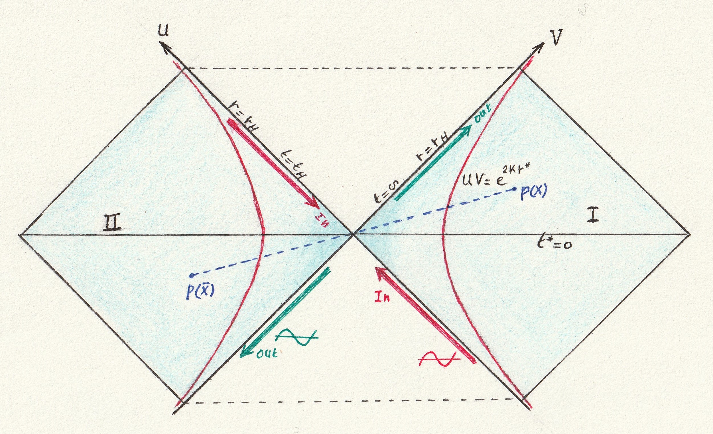
Figure 5: Penrose diagram. The antipodal points $P(X)$ and $P(\bar{X})$ are identified. Particles going in will generate waves approaching the horizon from the outside and passes the horizon, will reappear from "the other side" of the black hole. Note that $t^{*}=log(U/V)\sim log(t-t_{H})$.

Note that $ds^{2}$ and $H$ are invariant under $\tilde{U}\rightarrow-\tilde{U}$ and $\tilde{V}\rightarrow-\tilde{V}$. $\tilde{g}_{\mu\nu}$ is regular everywhere and conformally flat. Note that the hyperbolas in the Penrose diagram (see Figure B1) can be described by

$$UV=e^{2\kappa r^{*}}=(r-r_{H})^{\frac{\kappa r_{H}}{2(r_{H}+b_{2})^{3}}},$$ (111)

where $b_{2}$ contains the mass and $\kappa$ a constant. So when the black hole is evaporating, the hyperbola moves to the left in region I in the Penrose diagram. If $r$ is close to $r_{H}$, the hyperbola approaches the Planckian area.

Appendix C In $(U,V)$-coordinates

In light cone coordinates $u=r-t$ and $v=r+t$, one obtains a set of PDE’s

$$\Delta N=\frac{1}{1+N^{4}}\mathpzc{A},\quad\Delta\omega=\frac{1}{1-N^{4}}\mathpzc{B},\quad\Delta X=\frac{1}{1-N^{4}}\mathpzc{C},$$ (112)

where $\mathpzc{A},\mathpzc{B},\mathpzc{C}$ are expressions in $N,\omega,X$ and their derivatives. Further, $\Delta\equiv\partial_{u}^{2}+\partial_{v}^{2}$. These PDE’s can be used, in a numerical setting, in order to follow the Hawking particles in the $(U,V)$ plane. One also can proof that Laplace equations make sense on Klein surfacesalling1971

Appendix D Notations

$d$: spacetime dimension
$n$: topological windingnumber or Chern number
$(t,r,z,\varphi)$: coordinates of the 4D spacetime
$\mathpzc{y}$: fifth dimension in RS model
$y_{0}$: dimension of the bulk spacetime
$\Bigl{(}N(t,r),N^{\varphi}(t,r)\Bigr{)}$: metric components
${\cal V}$: $z+i\mathpzc{y}$
${\cal W}$: $x+iy$
${\cal Z}:\frac{{\cal V}}{{\cal W}}$
$\mathds{R}^{n}$: n-dimensional Euclidean space
$\mathds{C}^{n}$: complex n-dimensional space
$\eta$: vacuum expectation value
$\omega(t,r)$: dilaton field
$\Phi=\eta X(t,r)e^{in\varphi}$: complex scalar (Higgs) field
$A_{\mu}$: gauge field =$(0,0,0,A_{\varphi},0)$
$S^{m}$: m-sphere, $\{x\in\mathds{R}^{m+1}\mathchar 24635\relax\;|x|=1\}$
$B^{m}$: m-ball
$\mathds{R}P^{m}$: real projective m-space
$\mathds{C}P^{m}$: complex projected m-space
$\mathds{Z}_{2}$: reflection symmetry, i.e. a symmetry operation that yields the identity if applied twice
$\mathds{T}$: torus $S^{1}\times S^{1}$
$\mathds{K}:$ Klein surface = compact surface (i.e., triangulation possible) of the connected sum of two projective planes $\mathds{R}P^{1}\#\mathds{R}P^{1}$
$f:S^{2}\rightarrow\mathds{R}P^{1}$: map of 2-sphere onto its quotient space (or identification space topology)
$(S^{2},f)$: covering space of $\mathds{R}P^{1}$

Appendix E The Schrödinger equation and the multiple-scale method

E.1 The $\Phi^{4}$-Klein-Gordon equation

Consider the 1+1 dimensional Lagrangian density

$${\cal L}=\frac{1}{2}\Bigl{[}-\partial_{\mu}\Phi\partial^{\mu}\Phi-V(\Phi\Bigr{]},$$ (113)

with $V=\frac{1}{4}\beta(\Phi^{2}-\frac{\alpha}{\beta})^{2}$. From Euler-Lagrange equations we obtain the well-known $\Phi^{4}$ model

$$\Phi_{tt}-\Phi_{xx}=-(\beta\Phi^{2}-\alpha)\Phi.$$ (114)

Note that $-\frac{1}{2}\alpha\Phi^{2}$ is the mass term in the potential. The potential possesses two distinct minima, so we have a classical degenerated vacuum, $\Phi_{0}=\pm\sqrt{\frac{\alpha}{\beta}}$. At infinity, the field is static and the configuration must have finite energy. This results in boundary conditions

$$\Phi_{\pm\infty}=\lim_{x\rightarrow\pm\infty}\Phi(x,t)=\pm\sqrt{\frac{\alpha}{\beta}},\qquad U(\Phi_{\pm\infty})=0.$$ (115)

E.2 The "kink"-sector

The most simple topological soliton solution of the $\Phi^{4}$ model occur in one space dimension. Solutions interpolate between the two vacua $\Phi_{\pm}=\sqrt{\frac{\alpha}{\beta}}$. The topological "charge" is then

$$Q=\int_{-\infty}^{+\infty}\frac{\partial\Phi}{\partial x}dx=\Phi(+\infty,t)-\Phi(-\infty,t)=\frac{\Phi_{+}-\Phi_{-}}{2\sqrt{\frac{\alpha}{\beta}}},\quad Q=\{-1,0,1\}.$$ (116)

We see that $Q$ only depends on the asymptotic behavior at infinity. Note that in the related sine-Gordon model, one has an infinite series of discrete minima, (Q = 0…n) in contrast with the $\Phi^{4}$ model. So in this case Q is topologically quantized. However, in 2 space dimensions $(r,\varphi)$ in the axially symmetry, one has the topological quantization via the winding number.

One can wonder, if the vacuum degeneracy will survive the quantization. The answer is yes. The soliton solution is quantum-mechanically stable, i.e., cannot decay into one of the vacua.

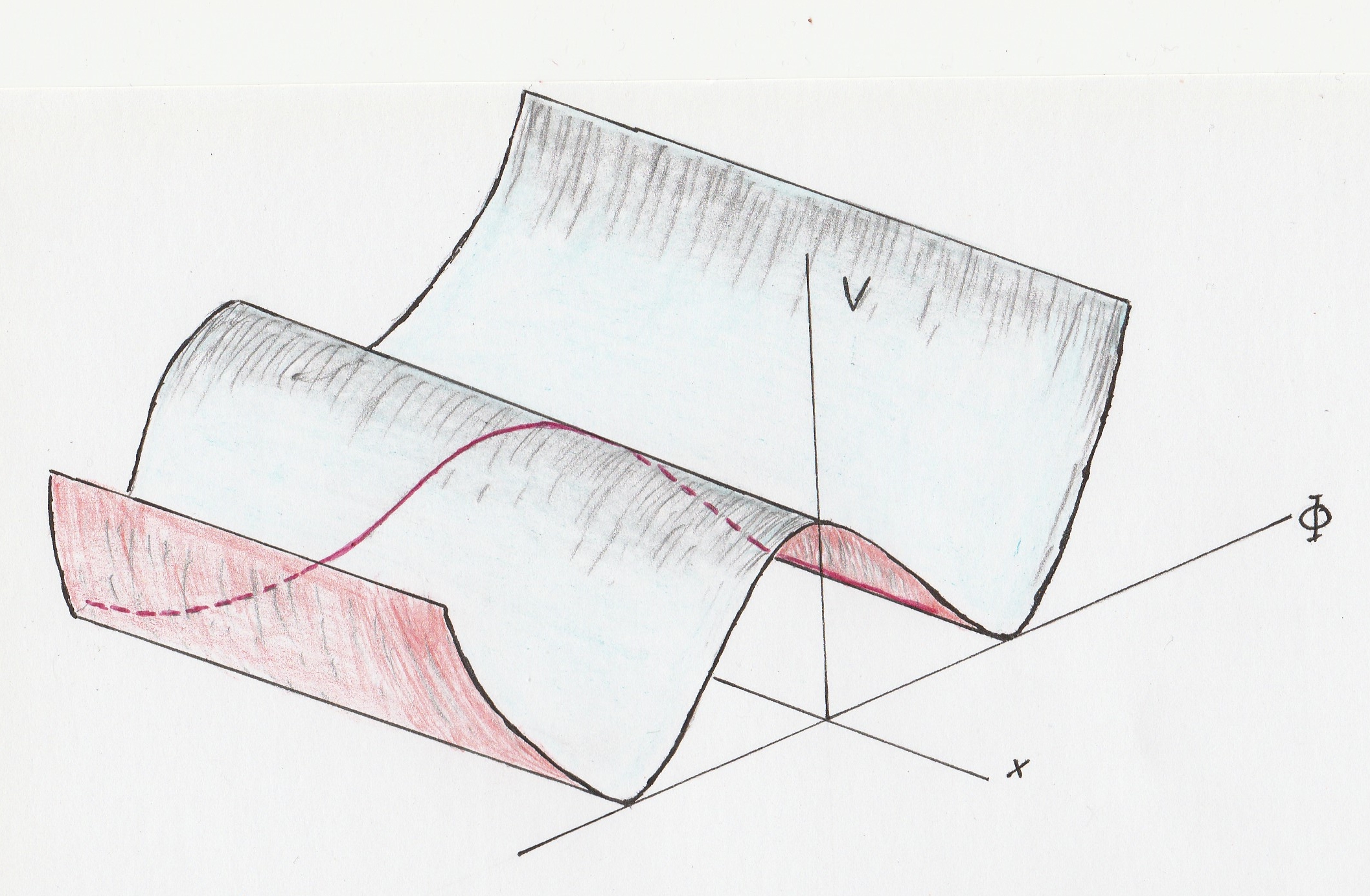
Figure 6: The $\Phi$-kink needs an infinite amount of energy in order to overcome the ridge of infinite length.

A traveling wave solution can easily be obtained.

If one wants a localized traveling wave solution of the form (solitary wave)

$$\Phi(x,t)=f(x-vt)=f(\xi),\qquad\lim_{\xi\rightarrow\pm\infty}f(\xi)=\Phi_{\pm\infty},$$ (117)

then one can write the equation as

$$\frac{df}{d\xi}=\pm\gamma\sqrt{2U[f]},\qquad\gamma=\frac{1}{\sqrt{1-v^{2}}},$$ (118)

or

$$\lambda(\xi-\xi_{0})=\pm\int\frac{df}{\sqrt{2U[f]}}.$$ (119)

It possesses the "kink" and "anti-kink"-solutions.

E.3 The method of multiple-scales

Let us expand

$$\Phi(x,t\mathchar 24635\relax\;\epsilon)=\sum_{1}^{\infty}\epsilon^{kp}\Phi^{(k)}(x,t\mathchar 24635\relax\;\epsilon)$$ (120)

with $\epsilon$ a small parameter. Introduce "slow" variables

$${\rm X}_{k}=\epsilon^{k}x,\qquad{\rm T}_{k}=\epsilon^{k}t,\quad k=1,2,..$$ (121)

So we write

$$\Phi(x,t\mathchar 24635\relax\;\epsilon)=\tilde{\Phi}(x,t,{\rm X}_{1},{\rm T}_{1},{\rm X}_{2},{\rm T}_{2},...\mathchar 24635\relax\;\epsilon)$$ (122)

and

$$\frac{\partial\Phi}{\partial x}=\frac{\partial\tilde{\Phi}}{\partial x}+\sum_{k=1}\epsilon^{k}\frac{\partial\tilde{\Phi}}{\partial{\rm X}_{k}},\qquad\frac{\partial\Phi}{\partial t}=\frac{\partial\tilde{\Phi}}{\partial t}+\sum_{k=1}\epsilon^{k}\frac{\partial\tilde{\Phi}}{\partial{\rm T}_{k}}$$ (123)

So $\epsilon$ measures the ratio of the fast scale to the slow scale. Substitution into Eq.(114) with also

$$\tilde{\Phi}(x,t,{\rm X}_{1},{\rm T}_{1},...\mathchar 24635\relax\;\epsilon)=\sum_{k=1}^{\infty}\epsilon^{kp}\tilde{\Phi}^{(k)}(x,t,{\rm X}_{1},{\rm T}_{1},...\mathchar 24635\relax\;\epsilon)$$ (124)

and equating coefficients of equal powers of $\epsilon$, results in:(tilde omitted):

1. term of ${\cal O}(\epsilon^{p})$

$$\epsilon^{p}\Bigl{(}\frac{\partial^{2}}{\partial x^{2}}-\frac{\partial^{2}}{\partial t^{2}}+\alpha\Bigr{)}\Phi^{(1)}$$ (125)

2. term of ${\cal O}(\epsilon^{p+1})$

$$2\epsilon^{p+1}\Bigl{(}\frac{\partial^{2}}{\partial x\partial{\rm X}_{1}}-\frac{\partial^{2}}{\partial t\partial{\rm T}_{1}}\Bigr{)}\Phi^{(1)}$$ (126)

3. term of ${\cal O}(\epsilon^{p+2})$

$$\epsilon^{p+2}\Bigl{(}\frac{\partial^{2}}{\partial{\rm X}_{1}^{2}}-\frac{\partial^{2}}{\partial{\rm T}_{1}^{2}}+2\frac{\partial^{2}}{\partial x\partial{\rm X}_{2}}-2\frac{\partial^{2}}{\partial t\partial{\rm T}_{2}}\Bigr{)}\Phi^{(1)}$$ (127)

4. term of ${\cal O}(\epsilon^{2p})$

$$\epsilon^{2p}\Bigl{(}\frac{\partial^{2}}{\partial x^{2}}-\frac{\partial^{2}}{\partial t^{2}}+\alpha\Bigr{)}\Phi^{(2)}$$ (128)

5. term of ${\cal O}(\epsilon^{2p+1})$

$$2\epsilon^{2p+1}\Bigl{(}\frac{\partial^{2}}{\partial x\partial{\rm X}_{1}}-\frac{\partial^{2}}{\partial t\partial{\rm T}_{1}}\Bigr{)}\Phi^{(2)}$$ (129)

6. term of ${\cal O}(\epsilon^{2p+2})$

$$\epsilon^{2p+2}\Bigl{(}\frac{\partial^{2}}{\partial{\rm X}_{1}^{2}}-\frac{\partial^{2}}{\partial{\rm T}_{1}^{2}}+2\frac{\partial^{2}}{\partial x\partial{\rm X}_{2}}-2\frac{\partial^{2}}{\partial t\partial{\rm T}_{2}}\Bigr{)}\Phi^{(2)}$$ (130)

7. term of ${\cal O}(\epsilon^{3p})$

$$\epsilon^{3p}\Bigl{(}(\frac{\partial^{2}}{\partial x^{2}}-\frac{\partial^{2}}{\partial t^{2}}+\alpha\Bigr{)}\Phi^{(3)}+\epsilon^{3p}\beta(\Phi^{(1)})^{3}$$ (131)

So to lowest order we get:

$$\boxed{\Bigl{(}\frac{\partial^{2}}{\partial x^{2}}-\frac{\partial^{2}}{\partial t^{2}}+\alpha\Bigr{)}\Phi^{(1)}=0}$$ (132)

This is the linearized equation. The next term is ${\cal O}(\epsilon^{p+1})$ and/or ${\cal O}(\epsilon^{2p})$. However $2p<(p+1)$ is impossible, because $p\in{\rm N}$. So for the next term we have $p+1<2p$ or $p+1=2p$. If $p+1=2p$ then $p=1$ and we have (we ignore for the moment the other possibility $p+1<2p,i.e.,p=2$ or 3 or 4, …) for the next order:

$$\Bigl{(}\frac{\partial^{2}}{\partial x^{2}}-\frac{\partial^{2}}{\partial t^{2}}+\alpha\Bigr{)}\Phi^{(2)}+2\Bigl{(}\frac{\partial^{2}}{\partial x\partial{\rm X}_{1}}-\frac{\partial^{2}}{\partial t\partial{\rm T}_{1}}\Bigr{)}\Phi^{(1)}=0$$ (133)

and

$$\Bigl{(}\frac{\partial^{2}}{\partial x^{2}}-\frac{\partial^{2}}{\partial t^{2}}+\alpha\Bigr{)}\Phi^{(3)}+\Bigl{(}\frac{\partial^{2}}{\partial{\rm X}_{1}^{2}}-\frac{\partial^{2}}{\partial{\rm T}_{1}^{2}}+2\frac{\partial^{2}}{\partial x\partial{\rm X}_{2}}$$ (134)

$$-2\frac{\partial^{2}}{\partial t\partial{\rm T}_{2}}\Bigr{)}\Phi^{(1)}-\beta(\Phi^{(1)})^{3}+2\Bigl{(}\frac{\partial^{2}}{\partial x\partial{\rm X}_{1}}-\frac{\partial^{2}}{\partial t\partial{\rm T}_{1}}\Bigr{)}\Phi^{(2)}=0$$ (135)

One can solve in principle Eq.(132)-Eq.(135). From Eq.(132) we have the solution

$$\Phi^{(1)}(x,t,{\rm X}_{1},{\rm T}_{1},{\rm X}_{2},{\rm T}_{2},...)=A^{(1)}({\rm X}_{1},{\rm T}_{1},{\rm X}_{2},{\rm T}_{2},...)e^{i\hbar(kx-\nu t)}+CC$$ (136)

with $\hbar^{2}(k^{2}-\nu^{2})=\alpha$ (dispersion relation), $k$ the wave number (number of oscillations per $2\pi$ in space) and $\nu$ the frequency (number of oscillations per $2\pi$ in time). Substitution in Eq.(133) yields

$$\boxed{\Bigl{(}\frac{\partial^{2}}{\partial x^{2}}-\frac{\partial^{2}}{\partial t^{2}}+\alpha\Bigr{)}\Phi^{(2)}=-2i\hbar\Bigl{(}k\frac{\partial A^{(1)}}{\partial{\rm X}_{1}}+\nu\frac{\partial A^{(1)}}{\partial{\rm T}_{1}}\Bigr{)}e^{i\hbar(kx-\nu t)}+CC}$$ (137)

The solution will contain a secular term of the form

$$B({\rm X}_{1},{\rm T}_{1},...)(kx-\nu t)e^{i\hbar(kx-\nu t)}$$ (138)

due to the fact of resonance with $e^{i\hbar(k^{\prime}x-\nu^{\prime}t)}$, which disturbs the asymptotic behavior. So we take

$$\Bigl{(}k\frac{\partial A^{(1)}}{\partial{\rm X}_{1}}+\nu\frac{\partial A^{(1)}}{\partial{\rm T}_{1}}\Bigr{)}=0$$ (139)

That means, $A^{(1)}$ will be of the form

$$A^{(1)}({\rm X}_{1},{\rm T}_{1},{\rm X}_{2},{\rm T}_{2},...)=A^{(1)}(\xi,{\rm X}_{2},{\rm T}_{2},...),$$ (140)

with

$$\xi\equiv{\rm X}_{1}-\frac{k}{\nu}{\rm T}_{1}.$$ (141)

So we have as first approximate solution of Eq.(114)

$$\Phi^{(1)}(x,t\mathchar 24635\relax\;\epsilon) = A^{(1)}\Bigl{(}{\rm X}_{1}-\frac{k}{\nu}{\rm T}_{1},{\rm X}_{2},{\rm T}_{2},...\Bigr{)}e^{i\hbar(kx-\omega t)}+CC$$ (142)

$$= A^{(1)}\Bigl{(}\epsilon(x-\frac{k}{\nu}t),\epsilon^{2}x,\epsilon^{2}t,...\Bigr{)}e^{i\hbar(kx-\omega t)}+CC$$ (143)

$$\approx A^{(1)}\Bigl{(}\epsilon(x-\frac{k}{\nu}t),0,0,...\Bigr{)}e^{i\hbar(kx-\nu t)}+CC.$$ (144)

We recognize the well-known carrier-wave (amplitude modulation)-solution: the amplitude varies slowly with respect to the wave $e^{i\hbar(kx-\nu t)}$. The envelope $A^{(1)}$ has a velocity of $\frac{k}{\nu}=\frac{d\nu}{dk}$, i. e., the velocity of the wave-packet.

Now we want to find the expression for $A^{(1)}$. From Eq.(137) and Eq.(139) we obtain

$$\Bigl{(}\frac{\partial^{2}}{\partial x^{2}}-\frac{\partial^{2}}{\partial t^{2}}+\alpha\Bigr{)}\Phi^{(2)}=0,$$ (145)

so a solution

$$\Phi^{(2)}=A^{(2)}({\rm X}_{1},{\rm T}_{1},{\rm X}_{2},{\rm T}_{2},...)e^{i\hbar(k^{\prime}x-\nu^{\prime}t)}+CC$$ (146)

with $\hbar^{2}(k^{\prime 2}-\nu^{\prime 2})=\alpha$. Substitution in Eq.(135) yields:

$$\Bigl{(}\frac{\partial^{2}}{\partial x^{2}}-\frac{\partial^{2}}{\partial t^{2}}+\alpha\Bigr{)}\Phi^{(3)}=-\Bigl{(}1-\frac{k^{2}}{\nu^{2}}\Bigr{)}\frac{\partial^{2}A^{(1)}}{\partial\xi^{2}}e^{i\hbar(kx-\omega t)}$$ (147)

$$-2i\hbar\Bigl{(}k\frac{\partial A^{(1)}}{\partial{\rm X}_{2}}+\nu\frac{\partial A^{(1)}}{\partial{\rm T}_{2}}\Bigr{)}e^{i\hbar(kx-\nu t)}-2i\hbar\Bigl{(}k^{\prime}\frac{\partial A^{(2)}}{\partial{\rm X}_{1}}+\nu^{\prime}\frac{\partial A^{(2)}}{\partial{\rm T}_{1}}\Bigr{)}e^{i\hbar(k^{\prime}x-\nu^{\prime}t)}$$ (148)

$$+\beta\Bigl{(}(A^{(1)})^{3}e^{3i(kx-\nu t)}+3(A^{(1)})^{2}\bar{A}^{(1)}e^{i(kx-\nu t)}\Bigr{)}+CC\qquad\qquad$$ (149)

Again we skip the secular terms:

$$1.\quad k^{\prime}\frac{\partial A^{(2)}}{\partial{\rm X}_{1}}+\nu^{\prime}\frac{\partial A^{(2)}}{\partial{\rm T}_{1}}=0$$ (150)

so we have

$$A^{(2)}({\rm X}_{1},{\rm T}_{1},{\rm X}_{2},{\rm T}_{2},...)=A^{(2)}(\xi^{\prime}.{\rm X}_{2},{\rm T}_{2},...),$$ (151)

with $\xi^{\prime}={\rm X}_{1}-\frac{k^{\prime}}{\nu^{\prime}}{\rm T}_{1}$, and

$$2.\quad\Bigl{(}1-\frac{k^{2}}{\nu^{2}}\Bigr{)}\frac{\partial^{2}A^{(1)}}{\partial\xi^{2}}+2i\hbar\Bigl{(}k\frac{\partial A^{(1)}}{\partial{\rm X}_{2}}+\nu\frac{\partial A^{(1)}}{\partial{\rm T}_{2}}\Bigr{)}-3\beta|A^{(1)}|^{2}A^{(1)}=0.$$ (152)

If we introduce the moving coordinate system (group-velocity $\frac{k}{\omega}$) $\xi_{2}={X}_{2}-\frac{k}{\nu}{T}_{2}$ and $T_{2}$, in order to get rid of $\partial X_{2}$, we obtain for the amplitude

$$A^{(1)}(\xi,\xi_{2},{\rm T}_{2},{\rm X}_{3},{\rm T}_{3},...)\approx A^{(1)}(\epsilon(x-\frac{k}{\nu}t),\epsilon^{2}(x-\frac{k}{\nu}t),\epsilon^{2}t,...)$$ (153)

the partial differential equation:

$$\boxed{i\hbar\frac{\partial A^{(1)}}{\partial{\rm T}_{2}}-\frac{\alpha}{2\hbar^{2}\nu^{3}}\frac{\partial^{2}A{(1)}}{\partial\xi_{2}^{2}}-\frac{3\beta}{2\nu}|A^{(1)}|^{2}A^{(1)}=0}.$$ (154)

which represents a cubic Schrödinger equation. We used the dispersion relation $k^{2}-\omega^{2}=\frac{\alpha}{\hbar^{2}}$. A typical solution is obtained for $\alpha=-2\hbar^{2}\omega^{3}$

$$A^{(1)}=C_{1}Exp\Bigl{[}i\Bigl{(}C_{2}\xi_{2}-(\frac{3\beta}{2\omega}C_{1}^{2}+C_{2}^{2})T_{2}+C_{3}\Bigr{)}\Bigr{]}$$ (155)

where $C_{i}$ are constants. So we have the first order approximation solution for $\Phi^{(1)}$

$$\boxed{\Phi^{(1)}(x,t\mathchar 24635\relax\;\epsilon)=\Phi^{(1)}(x,t,\xi,\xi_{2},T_{2},...)=C_{1}e^{i(C_{2}\xi_{2}-(\frac{3\beta}{2\omega}C_{1}^{2}+C_{2}^{2})T_{2}+C_{3})}e^{i\hbar(kx-\omega t)}+CC}$$ (156)

This form can be compared with the so-called "amplitude modulation". Now in our model, $\alpha$ is related to the mass in this $\Phi^{4}$ model. Other interesting solutions are

$$A^{(1)}=2C_{1}\sqrt{\frac{\omega}{3\beta}}\frac{e^{i(C_{1}^{2}T_{2}+C_{2})}}{\cosh(C_{1}\xi_{2}+C_{3})}$$ (157)

$$A^{(1)}=2C_{1}\sqrt{\frac{\omega}{3\beta}}\frac{e^{i\Bigl{(}C_{2}\xi_{2}+(C_{1}^{2}-C_{2}^{2})T_{2}+C_{1}\Bigr{)}}}{\cosh(C_{1}\xi_{2}-2C_{1}C_{2}T_{2}+C_{3})}$$ (158)

$$A^{(1)}=\frac{C_{1}}{\sqrt{T_{2}}}e^{i\Bigl{[}\frac{(\xi_{2}+C_{2})^{2}}{4T_{2}}+(\frac{3\beta}{2\omega}C_{1}^{2}\ln T_{2}+C_{3})\Bigr{]}}$$ (159)

We have now two scales, the slow $(\xi_{2},T_{2})$ and the fast $(t,x)$. Most of the solutions are obtained by the inverse-scattering method, the method of Zakharov-Shabat. Further, there are conserved quantities,

$$\int_{-\infty}^{+\infty}|\Phi|^{2}dx,\quad\int_{-\infty}^{+\infty}i(\bar{\Phi}\partial_{x}\Phi-\Phi\bar{\partial\Phi})dx,\quad\int_{-\infty}^{+\infty}\Bigl{(}|\partial_{x}\Phi|^{2}+\frac{3\beta}{4\omega}|\Phi|^{4}\Bigr{)}$$ (160)

It would be interesting to explore the case $p=2$.

E.4 Application to the Vaidya spacetime

One expands the relevant fields

$$V_{i}=\sum_{n=0}^{\infty}\frac{1}{\nu^{n}}F_{i}^{(n)}({\bf x},\xi),$$ (161)

where $\nu$ represents a dimensionless parameter ("frequency"), which will be large. Further, $\xi=\nu\Theta({\bf x})$, with $\Theta$ a scalar (phase) function on the manifold. The small parameter $\frac{1}{\nu}$ can also be the ratio of the characteristic wavelength of the perturbation to the characteristic dimension of the background. On warped spacetimes it could also be the ratio of the extra dimension to the background dimension. In the vacuum case, we expand the metric

$$g_{\mu\nu}=\bar{g}_{\mu\nu}+\frac{1}{\nu}h_{\mu\nu}({\bf x},\xi)+\frac{1}{\nu^{2}}k_{\mu\nu}({\bf x},\xi)+...,$$ (162)

where we defined

$$\frac{dg_{\mu\nu}}{dx^{\sigma}}=g_{\mu\nu,\sigma}+\nu l_{\sigma}\dot{g}_{\mu\nu},\quad g_{\mu\nu,\sigma}=\frac{\partial g_{\mu\nu}}{\partial x^{\sigma}},\quad\dot{g}_{\mu\nu}=\frac{\partial g_{\mu\nu}}{\partial\xi},$$ (163)

with $l_{\mu}=\frac{\partial\Theta}{\partial x^{\mu}}$. One then says that

$$V_{i}=\sum_{n=-m}^{\infty}\frac{1}{\nu^{n}}F_{i}^{(n)}({\bf x},\xi)$$ (164)

is an approximate wavelike solution of order n of the field equation, if $F_{i}^{(n)}=0,\forall n$. One can substitute the expansion into the field equations. The Ricci tensor then expands as

$$R_{\mu\nu}\rightarrow\omega R_{\mu\nu}^{(-1)}+\Bigl{(}\bar{R}_{\mu\nu}+R_{\mu\nu}^{(0)}\Bigr{)}+\frac{1}{\omega}R_{\mu\nu}^{(1)}+...$$ (165)

By equating the subsequent orders to zero, we obtain

$$R_{\mu\nu}^{(-1)}=0=\frac{1}{2}\bar{g}^{\beta\lambda}(l_{\lambda}l_{\mu}\ddot{h}_{\beta\nu}+l_{\nu}l_{\beta}\ddot{h}_{\mu\lambda}-l_{\lambda}l_{\beta}\ddot{h}_{\mu\nu}-l_{\nu}l_{\mu}\ddot{h}_{\beta\lambda}),$$ (166)

$$R_{\mu\nu}^{(0)}+\bar{R}_{\mu\nu}=0,\qquad R_{\mu\nu}^{(1)}=0,\qquad....$$ (167)

The bar stands for the background. Here we used $l_{\mu}l^{\mu}=0$. The rapid variation is observed in the direction of $l_{\mu}$. The eikonal condition, $l_{\mu}l^{\mu}=0$, in linear approximations, is adopted as gauge condition. In the high-frequency approximation, however, it follows from the highest order ($n=-1$) equations. In the radiative outgoing Eddington-Finkelstein coordinates, we have $x^{1}=u=\Theta({\bf x})=t-r$ and $l_{\mu}=(1,0,0,0)$.
=========================oOo==========================

References

• (1) S. Hawking, Particle creation by black holes, Comm. Math. Phys. 43, (1975) 199.
• (2) A. Almheiri, D. Marolf, J. Polchinski and J. Sully, Black holes: complementarity or firewalls?, JHEP 62, (2013) 62.
• (3) J. Maldacena and L. Susskind (2013), Cool horizons for entangled black holes, Fortsch. Phys., 61, (2013) 781811.
• (4) S. D. Mathur, The information paradox: a pedagogical introduction, Class. Quantum Grav., 26, (2009) 224001.
• (5) J. Foo, R. B. Mann and M. Zych, Schrรถdingerโ€™s cat for deSitter, Class. Quantum Grav. , 38, (2021) 115010.
• (6) J. D. Bekenstein, The quantum mass spectrum of the kerr black, Lettere al Nuovo Cimento , 11, (1974) 467.
• (7) P. Betzios, N. Gaddam and O. Papadoulaki, Black hole S-matrix for a scalar field, JHEP 17, (2021) 7.
• (8) G. โ€™t Hooft, Diagonalizing the black hole information retrieval process, arXiv: gr-qc/150901695 (2015).
• (9) G. โ€™t Hooft, Local conformal symmetry: the missing symmetry component for space and time, arXiv: gr-qc/14106675 (2015)
• (10) E. Schrรถdinger, Expanding universe, Cambridge University. Press, Cambridge U.K. (1957).
• (11) N. Sanchez and B. F. Whiting, Quantum field theory and the antipodal identification of black holes, Nucl. Phys. B283, (1987) 605.
• (12) N. Sanchez, Two- and four-dimensional semi-classical gravity and conformal mappings. Cern-Th.4592/86 (1998).
• (13) A. Folacci and N. Sanchez, Quantum field theory and the antipodal identification of de Sitter space. Elliptic inflation. NASA Astrophysical Data System, paper II.2 (1987).
• (14) G. W. Gibbons, The elliptic interpretation of black holes and quantum mechanics, Nuclear Physics, B271, (1986) 497.
• (15) G. โ€™t Hooft Black hole unitarity and antipodal entanglement, Found. Phys. 46, (2016) 1185.
• (16) G. โ€™t Hooft, Virtual black holes and spacetime structure, Found. Phys. 48, (2018) 1149.
• (17) G. โ€™t Hooft, The quantum black hole as a theoretical lab. arXiv: gr-qc/190210469 (2019).
• (18) G. โ€™t Hooft, The black hole firewall transformation and realism in quantum mechanics
• (19) G. ยดt Hooft, Quantum Clones inside black holes, Universe 8, (2022) 537.
• (20) M. Banฬ†ados, C. Teitelboim and T. Zanelli, The black hole in three-dimensional spacetime, Phys. Rev. Lett., 69, (1992) 1849.
• (21) R. J. Slagter, On the dynamical 4D BTZ black hole solution in conformally invariant gravity, J. Mod. Phys. 11, (2019) 1711.
• (22) R. J. Slagter, Alternative for black hole paradoxes, Int. J. Mod. Phys. A (to appear, doi.10.1142/S0217751X22501767) arXiv: gr-qc/220510437 (2022).
• (23) P. D. Mannheim, PT symmetry as a necessary and sufficient condition for unitary time evolution, Phil. Trans. Roy. Soc. Lond. A371, (2013) 20120060.
• (24) P. Betzios, N. Gaddam and O. Papadoulaki, The black hole S-matrix from quantum mechanics, JHEP 11, (2016) 131.
• (25) P. Betzios, N. Gaddam and O. Papadoulaki, Black holes, quantum chaos, and the Riemann hypothesis, SciPost Phys.Core 4, (2021) 32.
• (26) L. Randall and R. Sundrum, A large mass hierarchy from a small extra dimension, Phys. Rev. Lett. 83, (1999,) 3370.
• (27) L. Randall and R. Sundrum, An alternative to compactification, Phys. Rev. Lett. 83, (1999) 4690.
• (28) R. J. Slagter, The dilaton black hole on a conformal invariant five dimensional warped spacetime: paradoxes possibly solved? arXiv: gr-qc/220306506
• (29) R. J. Slagter, Conformal invariant gravity coupled to a gauged scalar field and warped spacetimes, Phys. Dark Universe, (2018) 24 100282.
• (30) R. J. Slagter, A New black hole solution in conformal dilaton gravity on a warped spacetime, J. Mod. Phys. 12, (2021) 1758.
• (31) P. D. Mannheim, Alternatives to dark matter and dark energy, Prog. Part. Nucl. Phys. 56, (2005) 340 [arXiv: astro-ph/0505266v2].
• (32) R. J. Slagter and S. Pan, A new fate of a warped 5D FLRW model with a U(1) scalar gauge field, Found. of Phys. 46, (2016) 1075.
• (33) J. Maldacena and A. Milekhin, Humanly traversable wormholes, Phys. Rev. D 103, (2021), 066007.
• (34) T. Shiromizu, K. Maeda and M. Sasaki, The Einstein equations on the 3-brane world, Phys. Rev. D 62, (2000) 024012.
• (35) T. Shiromizu, K. Maeda and M. Sasaki, Low energy effective theory for two branes system-covariant curvature formulation, Phys. Rev. D 7, (2003) 084022.
• (36) N. Gaddam and N. Groenenboom, Soft graviton exchange and the information paradox, arXiv: hep-th/2012.02355
• (37) N. Gaddam and N. Groenenboom, 2 โ†’ 2N scattering: Eikonalisation and the Page curve, JHEP 2022, (2022) 146.
• (38) N. Gaddam, N. Groenenboom and G. ยดt hooft, Quantum gravity on the black hole horizon, JHEP 2022, (2022) 23.
• (39) N. Gaddam and N. Groenenboom, A toolbox for black hole scattering, arXiv: hep-th/2207.11277 .
• (40) Y. Choquet-Bruhat, Constuction de solutions radiative approchรฉes des equations dโ€™Einstein, Commun. Math. Phys. 12, (1969) 16.
• (41) R. J. Slagter, Gravitational waves from spinning non-Abelian cosmic strings, Classical and Quantum Grav., 18, (2001) 463.
• (42) J. Abedi, H. Dykaar and N. Afshordi, Echoes from the Abyss: tentative evidence for Planck-scale structure at the black hole horizons, Phys. Rev., D 96, (2017) 082004 .
• (43) A. Codello, G. Dโ€™Odorico, G. Pagani and R. Percacci, The renormalization group and Weyl-invariance, Class. Quant. Grav. 30, (2013) 115015.
• (44) I. Oda, Conformal Higgs gravity, Adv. Studies in Theor. Phys. 9, (2015) 595.
• (45) E. Alvarez, M. Herrero-Valea and C. P. Martin, Conformal and non conformal dilaton gravity, JHEP 10, (2014) 214.
• (46) G. โ€™t Hooft, Singularities, horizons, firewalls and local conformal symmetry. arXiv: gr-qc/151104427 (2015).
• (47) B. Felsager, Geometry, particles and fields. Springer, New York. (1998).
• (48) R. J. Slagter, Conformal dilaton gravity and warped spacetimes in 5D . arXiv: gr-qc/201200409 (2021).
• (49) N. L. Alling and N. Greenleaf, Foundations of the Klein surfaces, Springer, Berlin, (1971).
• (50) R. Maartens and K. Koyama, Brane-world gravity, Liv. Rev. Rel. 13, (2010) 5.
• (51) A. Jaffe and C. Taubes, Vortices and monopoles. Structure of static gauge theories. Birkhรคuser, Boston, 1980.
• (52) N. A. Strauss, B. F. Whiting and A. T. Franzen, Classical tools for antipodal identification in Reissner-Nordstrom spacetime. arXiv: gr-qc/200202501 (2020).
• (53) H. K. Urbantke, The Hopf fibration-seven times in physics, J. Geom and Phys. 46, (2003) 125.
• (54) W. S. Massey, Algebraic topology: an introduction, Harcourt, brace & World, Inc. New York (1971).
• (55) P. Betzios, N. Gaddam and O. Papadoulaki, Black hole S-matrix for a scalar field, JHEP, 2021, (2021) 17.
• (56) D. Groisser and T. H. Parker, The Riemannian geometry of the Yang-Mills Moduli Space, Commun. Math. Phys. 112, (1987) 663.
• (57) S. L. Altmann, Rotations, quaternions and double groups, Clarendon Press, Oxford,(1986).
• (58) G. Toth, Finite Mรถbius groups, minimal immersions of spheres and Moduli, Springer, Heidelberg, (2002).
• (59) H. Urbantke, Two-level quantum systems: states, phases and holonomy, Am. J. Phys. 59, (1990) 503.
• (60) D. S. Freed and K. K. Uhlenbeck, Instantons and four-manifolds, Springer-Verlag, New York, (1984).
• (61) R. J. Slagter, New Evidence of the azimuthal alignment of quasars spin vector in the LQG U1.28, U1.27, U1.11, cosmologically explained, New Astronomy, 95 , (2022) 101797.