Quantum memory assisted observable estimation

Abstract

The estimation of many-qubit observables is an essential task of quantum information processing. The generally applicable approach is to decompose the observables into weighted sums of multi-qubit Pauli strings, i.e., tensor products of single-qubit Pauli matrices, which can readily be measured with single qubit rotations. The accumulation of shot noise in this approach, however, severely limits the achievable variance for a finite number of measurements. We introduce a novel method, dubbed coherent Pauli summation (CPS), that circumvents this limitation by exploiting access to a single-qubit quantum memory in which measurement information can be stored and accumulated. Our algorithm offers a reduction in the required number of measurements for a given variance that scales linearly with the number of Pauli strings in the decomposed observable. Our work demonstrates how a single long-coherence qubit memory can assist the operation of many-qubit quantum devices in a cardinal task.

1 Introduction

Quantum devices with on the order of hundreds of qubits have been realized with superconducting hardware [14, 17], neutral atoms [9, 19], and trapped ions [4, 35, 32]. These advancements stimulated interest in simulating many-body systems such as the electronic structure of molecules [2], studying non-equilibrium quantum statistical mechanics [42], and performing combinatorial optimization [7] on such devices. A cardinal task for many of these applications is to estimate the expectation values of many-qubit observables, such as the energy of the system. The direct estimation of such observables can be highly non-trivial for, e.g., fermionic observables simulated on qubit systems [23] and poses a significant challenge due to large measurement circuit depths and overall sampling complexity, i.e., the total number of measurements for a required estimation variance.

One approach for observable estimation with minimal sampling complexity is the quantum phase estimation (QPE) algorithm [16, 15, 37, 26, 41, 29]. Its implementation, however, requires qubit systems with low noise and long coherence times for high precision estimation since the measurement circuit depth is inversely proportional to the achievable precision.

As an alternative, the quantum energy (expectation) estimation (QEE) approach of decomposing the observable into a weighted sum of $N$ multi-qubit Pauli strings is commonly used in the variational quantum eigensolver [31]. While QEE minimizes the measurement circuit depth by requiring only a single layer of single-qubit rotations, it also suffers from increased sample complexity due to the accumulation of shot noise in the estimation procedure. Specifically, the expectation values of Pauli strings are estimated independently, and the observable is then calculated as a linear combination of these.

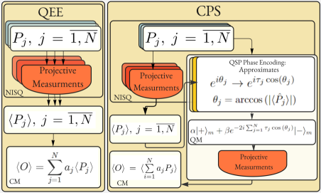
Figure 1: The comparison of the standard QEE method and the proposed CPS method. On the left, the QEE, where the expectation value of each Pauli string ($\langle\hat{P}_{j}\rangle$, $j=1,\dots,N$) is estimated by a series of projective measurements. Finally, an estimate of the observable $\langle\hat{O}\rangle$ is obtained by a weighted summation of all $\langle\hat{P}_{j}\rangle$. On the right, the CPS, where $\langle\hat{P}_{j}\rangle$ is encoded in the single qubit quantum memory (QM) such that a direct encoding of $\langle\hat{O}\rangle$ is obtained. To ensure the right summation of the Pauli strings in the phase of the memory qubit, quantum signal processing (QSP) is used for efficient approximation of the required function. In addition, a small amount of projective measurements of each Pauli string is also being performed for Pauli strings sign estimation ($\tau_{j}$) purposes. After the encoding process is done, a final projective measurement on the quantum memory qubit is performed. The procedure is then iterated to obtain an estimate of $\langle\hat{O}\rangle$ to the desired variance.

Consequently, to estimate an observable comprised of $N$ Pauli stings to a variance $\eta$, each Pauli string should be estimated to a variance $O(\eta/N)$ resulting in an overall sample complexity scaling as $O(N^{2})$. This accumulation of noise poses a “shot noise bottleneck" since the amount of measurements will ultimately be limited by the available runtime of the device before, e.g., re-calibration of the device is needed. The measurement process itself is also often one of the most time consuming operations in current quantum devices [14, 4, 35].

To tackle the shot noise bottleneck, recent works have considered intermediate approaches between QPE and QEE to obtain better variance in the estimation of the individual Pauli strings [40] or methods for grouping Pauli strings in commuting sets to reduce the sample complexity [8, 5]. While both approaches have the potential to reduce the overall sample complexity, neither improves the fundamental scaling of the noise accumulation with the number of Pauli strings in the observable decomposition.

Here, we propose a novel approach dubbed coherent Pauli summation (CPS) that overcomes the shot-noise bottleneck through the use of a single-qubit quantum memory (QM). Our method allows for a direct measurement of the multi-qubit observable by estimating the phase of the memory qubit at the end of the protocol. Hence, the accumulation of shot noise, originating from the summation of individually estimated mean values of Pauli strings in the QEE approach, is prevented. Importantly, this is obtained with a measurement circuit depth that scales only logarithmically with the required estimation variance, in contrast to the linear scaling of the QPE algorithm.

The critical point of CPS is to employ quantum signal processing (QSP) techniques to encode the mean value of Pauli strings in the phase of a single qubit quantum memory. The lack of shot noise accumulation results in a gain in the variance of the estimate compared to the QEE of $O(1/N)$, where $N$ is the number of Pauli strings in the observable decomposition. This gain can be understood as obtaining a Heisenberg limited scaling of the variance rather than the standard quantum limit scaling of the QEE. The necessary coherence time of the single memory qubit required for CPS scales linearly with $N$, while the required coherence time overhead of the quantum device only increases logarithmically with the required variance. The CPS thus outlines how a single long-coherence qubit memory can advance the performance of larger scale quantum devices.

2 CPS method

In order to set the stage of our algorithm, we first review the basic steps of the standard QEE approach (see also Fig. 1). The first step of the QEE approach for estimating the expectation value of an observable $\hat{O}$ for a given quantum state $|\Psi\rangle$, is to decompose it into a weighted sum of Pauli strings

$$\hat{O}=\sum\limits_{j=1}^{N}a_{j}\hat{P}_{j},$$ (1)

where $a_{j}$ are the (real) decomposition coefficients and $\hat{P}_{j}$ are the Pauli strings composed as tensor products of single qubit Pauli matrices and the identity. This decomposition is always possible since a collection of $d^{2}$ Pauli strings forms a complete operator basis for a $d$ dimensional Hilbert space. However, the number of Pauli strings, $N$, in the decomposition can be very large for a general multi-qubit observable. For example, when mapping fermionic systems onto qubit quantum devices, local fermionic observables can map to multi-qubit observables spanning the device [6, 28, 39].

In general, the state $|\Psi\rangle$ is repeatedly prepared, and the Pauli strings are measured sequentially via projective measurements to obtain estimates of every Pauli string: $\langle\hat{P}_{j}\rangle\equiv\langle\Psi|\hat{P}_{j}|\Psi\rangle$ [31, 24]. The mean value of the observable $\langle\hat{O}\rangle$ can be calculated classically after estimating all $\langle\hat{P}_{j}\rangle$, $j=1\ldots N$. This approach, however, suffers from the accumulation of shot noise from the individually estimated mean values of the Pauli strings, as described above. If each estimate $\langle\hat{P}_{j}\rangle$ is estimated with a variance $\sigma^{2}(\langle\hat{P}_{j}\rangle)\sim\eta_{p}$, the variance of the final estimate is $\sigma^{2}(\hat{\langle O\rangle})\sim N\eta_{p}$, assuming roughly equal weights of the $\hat{P}_{j}$ in the decomposition of $\hat{O}$.

We now outline the CPS method that circumvents this accumulation of shot noise (see Fig. 1). Let $|\Psi_{0}\rangle\equiv\hat{V}|\boldsymbol{0}\rangle$ be a quantum state of the multi-qubit device, where $\hat{V}$ is an invertible preparation circuit. The state $|\boldsymbol{0}\rangle$ denotes the state where all qubits are prepared in their ground state $\ket{0}$. Let $\langle\Psi_{0}|\hat{O}|\Psi_{0}\rangle=\langle\hat{O}\rangle$ be the expectation value we want to estimate within a variance of $\eta$. The three steps of the CPS are:

1. Obtain rough estimates of the mean values of every Pauli string $\langle\Psi_{0}|\hat{P}_{j}|\Psi_{0}\rangle=\langle\hat{P}_{j}\rangle$, $j=1,\dots,N$ by performing $O\left(\log{\left(\frac{N}{\sqrt{\eta}}\right)}\right)$ projective measurements similar to the QEE approach. This step estimates $s_{j}=\text{sign}{(a_{j}\langle\hat{P}_{j}\rangle)}$ i.e. the sign information of the Pauli strings.

2. In the second step, $s_{j}\epsilon|a_{j}\langle\hat{P}_{j}\rangle|$ is directly encoded in the phase of the single qubit memory using a modified phase-kickback algorithm [18] together with QSP techniques. Here, $\epsilon\in(0,1)$ is a tuning parameter that is used to circumvent the general "modulo $2\pi$" ambiguity of phase estimation, which we will detail below. The encoding is done sequentially for all Pauli strings in the decomposition, resulting in a final phase of $\sim\epsilon\langle\hat{O}\rangle$ followed by a projective measurement of the single qubit state.

3. The previous step is repeated a number of times with a varying parameter $\epsilon$ to obtain the final estimate of $\langle\hat{O}\rangle$. In particular, the procedure is repeated $M_{l}=\alpha+\gamma(d_{L}-l)$ times with $\epsilon\propto 2^{l}$ for $l=1,2,\dots,d_{L}$, $d_{L}=[\log_{2}{1/\eta}]$. The increasing powers of $\epsilon$ enable estimation of the digits of $\langle\hat{O}\rangle$, thereby circumventing the $2\pi$ ambiguity of the phase estimation. Analysing the upper bound of the variance of the estimate, in [15], the Heisenberg scaling with the best constant can be achieved by selecting $\alpha=3$ and $\gamma=1$ without any extra assumptions on $M_{l}$. In general, the Heisenberg scaling is obtained for any $\alpha>2$ and $\gamma>0$. For more details, please see Appendix B. The total amount of repetitions of the second step with different powers of $\epsilon$ is $M_{q}=\sum_{l=0}^{d_{L}}M_{l}$.

At the end of these three steps, $\langle\Psi_{0}|\hat{O}|\Psi_{0}\rangle$ can be estimated up to a variance of $\eta$ with an overall sample complexity of $N/\eta$. We have counted this scaling as the number of state preparation circuits $V$ required in the method, which also includes the extra state preparation circuits that are part of the QSP step as detailed below.

The second step, as defined above, is the main step of CPS, which we will now describe in detail. Let us define the state $|\Psi_{j}\rangle\equiv\hat{P}_{j}|\Psi_{0}\rangle$. Following the arguments of Ref. [40], we consider the unitary $\hat{U}_{P_{j}}=\hat{V}\hat{\Pi}_{0}\hat{V}^{\dagger}\hat{P}_{j}$, where $\hat{\Pi}_{0}=\hat{I}-2|\boldsymbol{0}\rangle\langle\boldsymbol{0}|$ is a multi-qubit reflection operator and $I$ is the identity operator. It is seen that the action of $\hat{\Pi}_{0}$ is to provide a $\pi$ phase only to the $|\boldsymbol{0}\rangle$ state. The action of $\hat{U}_{P_{j}}$ is a rotation by a principal angle $\theta_{j}=\arccos{(|\langle\Psi_{0}|\Psi_{j}\rangle|)}=\arccos{(|\langle\hat{P}_{j}\rangle|)}$ in the subspace spanned by $|\Psi_{0}\rangle$ and $|\Psi_{j}\rangle$. Consequently, the state $|\Psi_{0}\rangle$ can be written as an equal superposition of eigenstates $|\theta_{j}^{\pm}\rangle$ of $\hat{U}_{P_{j}}$ with eigenvalues $e^{\pm i\theta_{j}}$, respectively. If it is possible to project onto one of these eigenstates, the standard phase kickback method could be used to encode the phase $\theta_{j}$ into a single auxiliary qubit. A similar approach was considered in Ref. [40] to have a better estimation of each individual Pauli string. Such an approach, however, still suffers from the same accumulation of shot noise as the QEE method from the classical summation of the Pauli string estimates. In addition, efficient projection onto the eigenstates is only possible if the mean values are bounded away from zero.

The CPS method follows a different approach that allows for a direct encoding of the full observable $\hat{O}$ in order to circumvent the shot noise bottleneck. In addition, projection onto the eigenstates $|\theta_{j}^{\pm}\rangle$ is not required for the CPS method. To encode $s_{j}\epsilon|a_{j}\langle\hat{P}_{j}\rangle|=s_{j}\epsilon|a_{j}|\cos({\theta}_{j})$ (rather than $\theta_{j}$) in the phase of the memory qubit, we implement a unitary $\hat{\mathcal{U}}_{P_{j}}$, which transforms $\hat{U}_{P_{j}}$ through Quantum Signal Processing [20], such that $\hat{\mathcal{U}}_{P_{j}}\ket{\theta_{j}^{\pm}}=e^{i\tau_{j}\cos{(\theta_{j})}}\ket{\theta_{j}^{\pm}}$, where $\tau_{j}\equiv s_{j}\epsilon|a_{j}|$. By iterating the basic building block depicted in Fig. 2 only $n=O(\log{(1/\epsilon_{QSP})})$ times with the right choice of QSP phases $\phi_{1}\cdots\phi_{n}$, we compile a polynomial approximation of $\hat{\mathcal{U}}_{P_{j}}$ up to an error of $\epsilon_{QSP}$ (see Appendix A). We note that the implementation of the controlled version of $\hat{U}_{P_{j}}$ (c$\hat{U}_{P_{j}}$) does not require controlled versions of the preparation circuit $\hat{V}$ but only controlled versions of the Pauli string $\hat{P}_{j}$ and $\hat{\Pi}_{0}$ operators. The control qubit for both operators will be the quantum memory qubit, $\ket{\psi}_{m}$, such that if $\ket{\psi}_{m}=\ket{0}_{m}$ no operation is applied on the target qubits, while if $\ket{\psi}_{m}=\ket{1}_{m}$, the operation is applied.

Applying the QSP sequence on a (normalized) input state $\left(\alpha\ket{+}_{m}+\beta\ket{-}_{m}\right)\otimes\ket{\Psi_{0}}$ gives the (unnormalized) state

$$\frac{1}{\sqrt{2}}\left({\alpha}|+\rangle_{m}+{\beta}e^{-2i\tau_{j}\cos{(\theta_{j})}}|-\rangle_{m}\right)$$

$$\otimes(\ket{\theta^{+}_{j}}+e^{-in\theta_{j}}\ket{\theta^{-}_{j}})+\varepsilon_{QSP}(n)\ket{\xi},$$ (2)

where $\ket{\xi}$ is a general (normalized) error state, which can be an entangled state between the memory qubit and the qubits of the multi-qubit device.

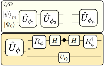
Figure 2: Quantum circuit realising the QSP by a sequence of controlled unitaries $\hat{U}_{\phi_{i}}(\theta_{j})$, $i=1,\dots,n$, built from Hadamard gates, $\hat{R}_{\phi}=e^{\frac{i\phi\hat{\sigma}_{z}}{2}}$, and controlled $\hat{U}_{P_{j}}$, $\ket{\psi}_{m}=\alpha\ket{+}_{m}+\beta\ket{-}_{m}$ denotes the state of a single memory qubit.

Method	Number of state preparations	Qubits	Coherence times
QEE	$N^{2}/\eta$	Processing qubits	$t_{prep}$
CPS	$(N/\eta)O\left(\frac{\log{(N/\sqrt{\eta})}}{\log{\log{(N/\sqrt{\eta})}}}\right)$	Processing qubits	$t_{prep}O(\log{(N/\sqrt{\eta})})$
		Memory qubit	$Nt_{prep}O\left(\frac{\log{(N/\sqrt{\eta})}}{\log{\log{(N/\sqrt{\eta})}}}\right)$

Table 1: Comparison of resources for the QEE and CPS methods for a fixed target variance $\eta$. We have quantified the necessary coherence times of the processing qubits of quantum device and the memory qubit in terms of the state preparation time, $t_{prep}$, which is assumed to be the dominant timescale. The observable is assumed to be decomposed into a summation of $N$ Pauli strings.

Repeating the above procedure for all Pauli strings in the decomposition of $O$ in a sequential manner, we prepare the single quantum memory (QM) qubit in a state

$$\approx {\alpha}|+\rangle_{m}+{\beta}e^{-2i\sum_{j=1}^{N}\tau_{j}\cos{(\theta_{j})}}|-\rangle_{m}$$ (3)

$$\approx {\alpha}|+\rangle_{m}+{\beta}e^{-2i\epsilon\langle O\rangle}|-\rangle_{m}$$

up to an error of $\sim N\varepsilon_{QSP}(n)$ assuming roughly the same approximation error for each Pauli string. Consequently, $\langle O\rangle$ is encoded in the phase of the QM qubit.

2.1 Phase wrapping

Since the phase encoding only provides an estimate of $\langle\hat{O}\rangle$ mod $2\pi$, we are facing a phase wrapping problem. To mitigate this issue, we have included the factor of $\epsilon$ in the encoding. This brings us to the third and final step of the CPS. To control the phase wrapping, we use the sampling approach introduced in Refs. [10, 15]. Instead of using fixed $\epsilon$ to encode $\theta_{j}$, we sample at multiple orders $\tilde{\epsilon}_{l}\equiv 2^{l}\epsilon$, $l=1,2,\dots,d_{L}$ to gradually enclose on $\langle\hat{O}\rangle$. This trick can be seen as sequentially estimating the digits of $\langle\hat{O}\rangle$. The parameter $\epsilon$ is selected in a way that $\sum_{j=1}^{N}s_{j}\epsilon|a_{j}|\cos{\theta_{j}}<2\pi$, holds. By a proper selection of $d_{L}$ and the number of measurements, we find that the CPS described above results in an estimate of $\hat{O}$ with a variance of $\sigma^{2}(\hat{O}_{CPS})\sim NT^{-1}$, where $T$ is the total number of state preparation circuits ($\hat{V}$ and $\hat{V}^{\dagger}$) necessary for all steps. The detailed analyses leading to this result can be found in Appendix B.

3 Resources comparison

In Tab. 1, we compare the required resources for the QEE and CPS methods: the required coherence time and the number of state preparation circuits. The coherence time is quantified by the duration of the state preparation circuit, $t_{prep}$, which can also be seen as a measure for the maximum circuit depth. The scaling of the number of state preparations is the proper indicator for the complexity of the CPS method when the cost of implementing controlled reflection and Pauli operations does not scale faster than that of state preparation. This requirement is satisfied easily for the controlled Pauli operation when the $\hat{P}_{j}$ are $k$-local. On the other hand, the controlled reflection operation can be implemented using resources that scales linearly in the number of qubits on the Rydberg atom platform [25, 12, 43, 38].

The QEE only requires a coherence time of the multi-qubit device of $\sim t_{prep}$ since after each state preparation, the qubits are measured. In comparison, the CPS requires a modest increase in the coherence time of the quantum device that scales logarithmic with the number of Pauli strings and the target variance, $\eta$. In return, the CPS provides a much better estimate of $\langle O\rangle$ than the QEE for a fixed number of state preparations. We find that

$$\frac{\sigma^{2}{(\hat{O}_{CPS})}}{\sigma^{2}{(\hat{O}_{QEE})}}\sim\frac{1}{N},$$ (4)

which shows that the CPS achieves a Heisenberg-like scaling of the variance in the number of Pauli strings compared to the standard quantum limit scaling of the QEE.

The limiting factor of both QEE and QSP will be the accumulation of operational errors in the final estimate of the observable. For both approaches, gate errors will reduce the accuracy of the final estimate of the observable. This reduction will have the same linear dependence on the number of Pauli strings in the observable decomposition for both approaches (see Appendix C). For the estimation of observable such as the energy of a $\text{H}_{3}^{+}$ molecule, which can be decomposed into $N\sim 59$ Pauli strings [5] on $4$ qubits, an estimate of the energy with a variance of $\eta\sim 1$ could be obtained for gate error probabilities around $\sim 0.5\cdot 10^{-3}$ and $10^{2}$ state preparations using CPS. In comparison, QEE would require $\sim 10^{3}$ state preparations to reach a similar variance. We do note, however, that the QEE approach would only require gate error probabilities on the order of $5\cdot 10^{-3}$ (we refer to Appendix D for more details). To simulate larger molecules, the performance of current hardware needs to be improved for both our method and QEE. For example, the CPS simulation of a LiH molecule with a decomposition of $\sim 630$ Pauli strings on $10$ qubits, requires $\sim 10^{3}$ state preparations and gate error probabilities $\sim 10^{-5}$, while the QEE method requires $\sim 10^{5}$ state preparations and gate error probabilities $\sim 10^{-4}$ to achieve the same variance of $\eta\sim 1$. Note, however, that the estimates for the required gate error probabilities are conservative since we assuming that just a single error corrupts the estimation. For specific implementations and hardware models better bounds can likely be obtained.

4 Summary

In summary, we propose a new method (CPS) to estimate the expectation values of multi-qubit observables. The method uses the QSP technique to encode information from a multi-qubit processor into a single qubit quantum memory, which allows to overcome the shot noise bottleneck of the conventional QEE. Compared to the QEE, the CPS obtains an Heisenberg limited scaling of the estimation variance with the number of Pauli strings in the decomposition of the observable. This scaling represents an improvement of $\leavevmode\nobreak\ 1/N$ compared to the QEE. We note that this improvement has been estimated assuming that there is on the order of $N$ non-commuting Pauli strings in the observable decomposition. If there are commuting sets of Pauli strings they can in principle be measured in parallel using the QEE while the CPS does not straightforwardly support parallel encoding of commuting Pauli strings. Thus, we imagine that potential trade-offs between commuting sets and non-commuting set of Pauli strings can be made, resulting in optimal strategies consisting of both methods depending on the specific observable.

While the CPS is designed for the estimation of a general observable, we believe that it will, in particular, be relevant for algorithms such as the variational quantum eigensolver where the observable is the energy of the system. In particular, for estimating molecular energies where the mapping from a fermionic system to a qubit system often introduces highly non-local terms and large Pauli string representations. We believe that platforms with native multi-qubit controlled gates such as Rydberg atoms [43, 38, 30] or systems with coupling to a common bus mode such as a cavity [3, 36] would be particularly suited due to their potential for implementing the controlled unitaries required for the CPS.

Finally, we note that another algorithm, which also uses QSP techniques to tackle the shot-noise bottleneck was recently proposed in Ref. [11]. Here $\tilde{O}(\sqrt{N/\eta})$ (where $\tilde{O}(\cdot)$ is used to hide the logarithmic factors) state preparations are needed to obtain an estimate within a variance of $\eta$ but $O(N\log{(N/\sqrt{\eta})}+N)$ ancillary qubits and a circuit depth of $\tilde{O}(1/\sqrt{\eta})$ are required. Reducing the amount of ancillary qubits to $O(N+\log{(1/\sqrt{\eta})})$, the same variance can be achieved with $\tilde{O}(N/\sqrt{\eta})$ state preparation queries, which is similar to the CPS method. However, the CPS method requires only one auxiliary memory qubit.

Appendix A CPS method

In this section, we first provide an overview of the basic notion of Quantum Signal Processing (QSP) [20] for the introduction of the Coherent Pauli Summation (CPS) method.

Let us consider a single qubit rotation of the form

$$\hat{R}_{\phi}(\theta)=e^{-i\frac{\theta}{2}(\hat{\sigma}_{x}\cos{\phi}+\hat{\sigma}_{y}\sin{\phi})}$$ (5)

with an angle $\theta$. This rotation can be considered as a computational module that computes a unitary function that depends on the selected parameter $\theta$, the input state and the measurement basis. A sequence of such $n$ single qubit rotations can be expressed as

$$\hat{R}_{\phi_{n}}(\theta)\dots\hat{R}_{\phi_{2}}(\theta)\hat{R}_{\phi_{1}}(\theta)=A(\theta)I+iB(\theta)\hat{\sigma}_{z}+iC(\theta)\hat{\sigma}_{x}+iD(\theta)\hat{\sigma}_{y}.$$ (6)

With a specific choice of different parameters $\vec{\phi}$, it is possible to compute more general functions of $\theta$ in terms of $A(\theta)$, $B(\theta)$, $C(\theta)$, and $D(\theta)$ being polynomials of, at most, degree $n$. Often it is enough to use a partial set of $(A,B,C,D)$, for example $(A,C)$ (see Ref. [21] for more details). For this operation, the following theorem holds

Theorem 1

[21] For any even $n>0$, a choice of real functions $A(\theta)$, $C(\theta)$ can be implemented by some $\vec{\phi}\in R^{n}$ if and only if all these are true:

• For any $\theta\in R$,

  $$A^{2}(\theta)+C^{2}(\theta)\geq 1,\quad\text{and}\quad A(0)=1,$$ (7)

• $A(\theta)=\sum\limits_{k=0}^{n/2}a_{k}\cos{(k\theta)}$, $\{a_{k}\}\in R^{n/2+1}$, $C(\theta)=\sum\limits_{k=0}^{n/2}c_{k}\cos{(k\theta)}$, $\{c_{k}\}\in R^{n/2}$.

Moreover, $\vec{\phi}$ can be efficiently computed from $A(\theta)$, $C(\theta)$.

Furthermore, given a unitary $\hat{U}$ with eigenstates $\hat{U}|\Psi_{0}\rangle=\frac{1}{\sqrt{2}}\sum_{\pm}e^{\pm i\theta}|\theta_{\pm}\rangle$, a quantum circuit $\hat{\mathcal{U}}=\sum_{\pm}e^{ih(\pm\theta)}|\theta_{\pm}\rangle\langle\theta_{\pm}|$ can be constructed, where $h(\theta)$ is a real function. To this end we need a $\vec{\phi}$ dependent version of $\hat{U}$, namely

$$\hat{U}_{\phi}=(e^{-i\frac{\phi}{2}\hat{\sigma}_{z}}\otimes\hat{1})\hat{U}_{0}(e^{i\frac{\phi}{2}\hat{\sigma}_{z}}\otimes\hat{1}),$$ (8)

$$\hat{U}_{0}=\sum\limits_{\pm}e^{\pm i\theta/2}\hat{R}_{0}(\pm\theta)\otimes\ket{\theta_{\pm}}\bra{\theta_{\pm}}.$$

An operator $\mathcal{\hat{V}}=\hat{U}_{\phi_{n}}\hat{U}_{\phi_{n-1}}\dots\hat{U}_{\phi_{1}}$ approximating $\hat{\mathcal{U}}$ is introduced. Applying it to the input state $\ket{+}\ket{\theta_{\pm}}$ and post selecting on measuring $\bra{+}$, we get $\bra{+}\mathcal{\hat{V}}\ket{+}\ket{\theta_{\pm}}=(A(\theta_{\pm})+iC(\theta_{\pm}))\ket{\theta_{\pm}}$ with the worst case success probability $p=\min\limits_{\theta}{|\langle+|\mathcal{\hat{V}}|+\rangle|^{2}}=\min\limits_{\theta}{|A(\theta_{\pm})+iC(\theta_{\pm})|^{2}}$. The second theorem holds:

Theorem 2

(quantum signal processing)[21] Any real odd periodic function $h:(-\pi,\pi]\longrightarrow(-\pi,\pi]$ and even $n>0$, let $A(\theta),C(\theta)$ be real Fourier series in $\cos{(k\theta)}$, $\sin{(k\theta)}$, $k=0,\dots,n/2$, that approximate

$$\max\limits_{\theta\in R}{|A(\theta)+iC(\theta)-e^{ih(\theta)}|}\leq\varepsilon_{QSP}.$$ (9)

Given $A(\theta),C(\theta)$, one can efficiently compute $\vec{\phi}$ such that $\langle+|\mathcal{\hat{V}}|+\rangle$ applies $\hat{U}_{\phi}$ a number $n$ times to approximate $\hat{\mathcal{U}}$ with success probability $p\geq 1-16\varepsilon_{QSP}$ and the distance $\max\limits_{\ket{\Psi}}{\|(\langle+|\mathcal{\hat{V}}|+\rangle-\hat{\mathcal{U}})\ket{\Psi_{0}}\|}\leq 8\varepsilon_{QSP}$.

At this point, we note that we are not conditioning on a projection onto the $\ket{+}$ state in the CPS method. Consequently, the notion of a success probability $p$ is not really valid in the CPS method and $p$ instead turns into an error of the approximation of the unitary by the QSP method, as we will show below. For now, we, however, keep the notion of success probability to relate to existing literature.

The query complexity of the methodology is exactly the degree $n$ of optimal trigonometric polynomial approximations to $e^{ih(\theta)}$ with error $\varepsilon_{QSP}$. It is mentioned, that $A(\theta)$, $C(\theta)$ satisfying the second theorem, in general, do not satisfy (7). Thus the rescaling is provided

$$A_{1}(\theta)=A(\theta)/(1+\varepsilon_{QSP}),\quad C_{1}(\theta)=C(\theta)/(1+\varepsilon_{QSP}),$$ (10)

$$|A_{1}(\theta)+iC_{1}(\theta)-e^{ih(\theta)}|\leq\varepsilon_{QSP}/(1+\varepsilon_{QSP})+\varepsilon_{QSP}<2\varepsilon_{QSP}.$$

Hence, the success probability of the method is at least $1-2\varepsilon_{QSP}$. We select $h(\theta_{j})=\tau_{j}\cos{(\pm\theta_{j})}$, $\tau_{j}=s_{j}\epsilon|a_{j}|$, $\epsilon\in(0,1)$, $s_{j}=\text{sign}({a_{j}\langle P_{j}\rangle)}$ and the input is $\theta_{j}=\arccos{(|\langle P_{j}\rangle|)}$. Then for every $\theta_{j}$, we can write

$$A(\theta)=\cos{(\tau\cos{(\theta)})},\quad C(\theta)=\sin{(\tau\cos{(\theta)})}.$$ (11)

We can use the real-valued Jacobi-Anger expansion [1] to rewrite the later functions as series:

$$\cos(\tau\cos{(\theta)})\equiv J_{0}(\tau)+2\sum_{m=1}^{\infty}(-1)^{m}J_{2m}(\tau)\cos(2m\theta),$$ (12)

$$\sin(\tau\cos{(\theta)})\equiv-2\sum_{m=1}^{\infty}(-1)^{m}J_{2m-1}(\tau)\cos\left[\left(2m-1\right)\theta\right],$$

where $J_{m}(\tau)$ is the $m$-th Bessel function of the first kind. The Bessel function $J_{m}(\tau)$ is bounded, for real $\tau$ and integer $n$ as

$$|J_{m}(\tau)|\leq\frac{1}{|m|!}\Big{|}\frac{\tau}{2}\Big{|}^{|m|}.$$ (13)

Under the conditions $|\tau|\leq k$ and $l!>(l/e)^{l}$ we can introduce the upper bound

$$2\sum_{m=k+1}^{\infty}|J_{m}(\tau)|\leq 4\sum_{m=k+1}^{\infty}\frac{1}{|m|!}\Big{|}\frac{\tau}{2}\Big{|}^{|m|}<\frac{4}{(k+1)!}\Big{|}\frac{\tau}{2}\Big{|}^{k+1}<4\Big{|}\frac{e\tau}{2(k+1)}\Big{|}^{k+1}.$$ (14)

Thus, we can truncate the series (12) at some point $k>n/2$ and keep the first $k$ terms. The error of the approximation of every $\exp{(i\tau_{j}\cos{[\arccos{(|\langle P_{j}\rangle|)}]})}$, $j=1,\dots,N$ is scaled super-exponentially as

$$\varepsilon_{QSP}\leq O\left(\left(\frac{e\tau}{2(k+1)}\right)^{k+1}\right),$$ (15)

where

$$|\tau|\leq k=n/2,$$ (16)

holds. Taking $k=e(\tau+\gamma)/2$, where $\gamma>0$ and $\tau=O(\gamma)$ we get the following amount of quarries [21]:

$$n_{QSP}\equiv n=O\left(\frac{\log{(1/\varepsilon_{QSP})}}{\log{\log{(1/\varepsilon_{QSP})}}}\right).$$ (17)

If we select $\ket{+}_{m}\otimes\ket{\Psi_{0}}$ as the initial state the action of the ideal QSP unitary $\mathcal{U}^{{\rm ideal}}_{P_{j}}$ on this state is the following

$$\hat{\mathcal{U}}^{{\rm ideal}}_{P_{j}}\ket{+}_{m}\otimes\ket{\Psi_{0}}=\ket{+}_{m}\otimes\sum\limits_{\pm}e^{i\tau_{j}\cos{(\pm\theta_{j})}}\ket{\theta_{\pm}}.$$ (18)

Note that $\ket{\Psi_{0}}$ is an equal superposition of two eigenstates $\ket{\theta_{j}^{\pm}}$ of $U_{P_{j}}$, with the eigenvalues $\pm\theta_{j}$, respectively. However, since $\mathcal{U}_{P_{j}}^{\rm ideal}$ has eigenvalues that are cosine transforms of the eigenvalues of $U_{P_{j}}$, the initial state $\ket{\Psi_{0}}$ is invariant under the action of $\mathcal{U}_{P_{j}}^{\rm ideal}$. Moreover, according the Theorem 2, choosing the initial state of the ancilla as $\ket{+}_{m}$, we select the functional transformation given by $A(\theta)+iC(\theta)$.

On the other hand, choosing the initial state of the ancillary qubit as $\ket{-}_{m}$, we obtain

$$\mathcal{U}^{{\rm ideal}}_{P_{j}}\ket{-}_{m}\otimes\ket{\Psi_{0}}=\ket{-}_{m}\otimes\sum\limits_{\pm}e^{-i\tau_{j}\cos{(\pm\theta_{j})}}\ket{\theta_{\pm}}.$$ (19)

In this case the functional transformation we select is $A(\theta)-iC(\theta)$. Hence, setting the initial state of the memory ancilla as

$$\ket{\psi}_{m}=\alpha\ket{+}_{m}+\beta\ket{-}_{m},$$ (20)

we have the following action

$$\mathcal{U}^{{\rm ideal}}_{P_{j}}\ket{\psi}_{m}\otimes\ket{\Psi_{0}}=\alpha\ket{+}_{m}\otimes\sum\limits_{\pm}e^{i\tau_{j}\cos{(\pm\theta_{j})}}\ket{\theta_{j}^{\pm}}+\beta\ket{-}_{m}\otimes\sum\limits_{\pm}e^{-i\tau_{j}\cos{(\pm\theta_{j})}}\ket{\theta_{j}^{\pm}}.$$ (21)

Repeating the QSP encoding for each Pauli string $P_{j}$, we encode the observable mean $\langle O\rangle$ in the phase of the memory qubit.

If we could approximate $h(\theta)$ perfectly, the phase encoded in the memory qubit would be the following

$$\Theta_{j}\equiv\tau_{j}|\langle P_{j}\rangle|.$$ (22)

However, since QSP method is just approximating the function from the random variable, we have to take into account the error emerging in the QSP approximation:

$$\Big{|}f_{QSP}\left(\arccos{(|\langle P_{j}\rangle|)}\right)-\exp{\left(i\Theta_{j}\right)}\Big{|}<\varepsilon_{QSP},$$ (23)

where $f_{QSP}$ is the approximation of $\exp{\left(i\tau_{j}\cos{(\cdot)}\right)}$. Then we can write

$$f_{QSP}\left(\arccos{(|\langle P_{j}\rangle|)}\right)=\exp{(i\Theta_{j})}\pm r_{j}\exp{(i\delta_{j})},$$ (24)

where $|r_{j}\exp{(i\delta_{j})}|<\varepsilon_{QSP}$, $\delta_{j}\in[0,2\pi)$, $r_{j}\in R$ is an error inserted by the QSP approximation.

Let us estimate the effect of this error on the variance of the estimate of $O$. We consider the input state $(\alpha\ket{+}_{m}+\beta\ket{-}_{m})\ket{\Psi_{0}}$. After $N$ full QSP rounds, we get the final state stored in the memory qubit:

$$|{\Phi}_{N}\rangle = \Bigg{(}(e^{i\Theta_{1}}\pm r_{1}e^{i\delta_{1}})(e^{i\Theta_{2}}\pm r_{2}e^{i\delta_{2}})\dots(e^{i\Theta_{N}}\pm r_{N}e^{i\delta_{N}})\alpha\ket{+}_{m}$$

$$+ (e^{-i\Theta_{1}}\pm r_{1}e^{-i\delta_{1}})(e^{-i\Theta_{2}}\pm r_{2}e^{-i\delta_{2}})\dots(e^{-i\Theta_{N}}\pm r_{N}e^{-i\delta_{N}})\beta\ket{-}_{m}\Bigg{)}|\theta_{1}^{N}\rangle,$$

where we used the notation

$$|\theta_{1}^{N}\rangle\equiv(|\theta_{1}^{+}\rangle+e^{-in\theta_{1}}|\theta_{1}^{-}\rangle)(|\theta_{2}^{+}\rangle+e^{-in\theta_{2}}|\theta_{2}^{-}\rangle)\dots(|\theta_{N}^{+}\rangle+e^{-in\theta_{N}}|\theta_{N}^{-}\rangle),$$ (26)

where $n$ scales as (17). Let us for simplicity select all signs to be plus, then we can rewrite the latter state as follows

$$|{\Phi}_{N}\rangle = \Bigg{(}\left(e^{i{\Phi}_{N}}+A\right)\alpha\ket{+}_{m}+\left(e^{-i{\Phi}_{N}}+B\right)\beta\ket{-}_{m}\Bigg{)}|\theta_{1}^{N}\rangle,$$ (27)

where we used the notations ${\Phi}_{N}=\sum\limits_{j=1}^{N}\Theta_{j}$ and

$$A\equiv\sum\limits_{j=1}^{N}r_{j}e^{i\delta_{j}}e^{i\sum\limits_{k=1,k\neq j}^{N}\Theta_{k}}+\sum_{\begin{subarray}{c}j,k=1,\\ j\neq k\end{subarray}}^{N}r_{j}r_{k}e^{i(\delta_{j}+\delta_{k})}e^{i\sum\limits_{r=1,r\neq j,k}^{N}\Theta_{r}}+\dots+(r_{1}r_{2}\dots r_{n})e^{i\sum\limits_{j=1}^{N}\delta_{j}},$$ (28)

and $B$ is the same expression but with the minus sign in the exponential functions. We rewrite the state in Eq. (27) as

$$|{\Phi}_{N}\rangle=e^{\Phi_{N}}\left(\alpha\ket{+}_{m}+\beta e^{-2i\Phi_{N}}\ket{-}_{m}\right)\otimes|\theta_{1}^{N}\rangle+(A\alpha\ket{+}_{m}+B\beta\ket{-}_{m})\otimes|\theta_{1}^{N}\rangle,$$ (29)

and in the main text of the article we denote it as

$$\left({\alpha}|+\rangle_{m}+{\beta}e^{-2i\sum_{j=1}^{N}\tau_{j}\cos{\theta_{j}}}|-\rangle_{m}\right)\otimes|\theta_{1}^{N}\rangle+\varepsilon_{QSP}(n)\ket{\xi},$$ (30)

where the second term is arising from the imperfection of the QSP approximation process. The notations we use are $\theta_{j}\equiv\arccos{(|\langle\hat{P}_{j}\rangle|)}$, $\tau_{j}\equiv\text{sign}{(a_{j}\langle\hat{P}_{j}\rangle)}\epsilon|a_{j}|$.

For the further calculation of the variance, where we are interested in the rate in $N$, we assume, for simplicity, $r_{j}=r$ and $\delta_{j}=\delta$, hold for all $j=1,\dots,N$. The series $A$ can be always written as

$$A = C_{N}^{1}re^{i\delta}e^{i\sum\limits_{k=1,k\neq 1}^{N}\Theta_{k}}+C_{N}^{2}r^{2}e^{2i\delta}e^{i\sum\limits_{r=1,r\neq 1,2}^{N}\Theta_{r}}+\dots+C_{N}^{N}r^{N}e^{iN\delta}=Re^{i\Theta_{R}},$$ (31)

$$R = \sqrt{\sum\limits_{j=1}^{N}(C_{j}^{N}r^{j})^{2}+2\sum\limits_{j,k=1,j\neq k}^{N}C_{N}^{j}C_{N}^{k}r^{j}r^{k}\cos{\left(i\left((j-k)\delta+\sum\limits_{r=1,r\neq j}^{N}\Theta_{r}-\sum\limits_{r=1,r\neq k}^{N}\Theta_{r}\right)\right)}},$$ (32)

$$\tan{(\Theta_{R})} = \frac{C_{N}^{1}r\sin{(\delta+\sum\limits_{k=1,k\neq 1}^{N}\Theta_{k})}+C_{N}^{2}r^{2}\sin{(2\delta+\sum\limits_{r=1,r\neq 1,2}^{N}\Theta_{r})}+\dots+C_{N}^{N}r^{N}\sin{(N\delta)}}{C_{N}^{1}r\cos{(\delta+\sum\limits_{k=1,k\neq 1}^{N}\Theta_{k})}+C_{N}^{2}r^{2}\cos{(2\delta+\sum\limits_{r=1,r\neq 1,2}^{N}\Theta_{r})}+\dots+C_{N}^{N}r^{N}\cos{(N\delta)}},$$ (33)

where $C_{N}^{k}$ are the binomial coefficients, $N\geq k\geq 0$. Hence, the later expression can be bounded by

$$\Big{|}Re^{i\Theta_{R}}\Big{|}<\sqrt{\sum\limits_{j=1}^{N}(C_{j}^{N}\varepsilon_{QSP}^{j})^{2}+2\sum\limits_{j,k=1,j\neq k}^{N}C_{k}^{N}C_{j}^{N}\varepsilon_{QSP}^{j+k}}=\sum\limits_{j=1}^{N}C_{j}^{N}\varepsilon_{QSP}^{j}=(1+\varepsilon_{QSP})^{N}-1\sim N\varepsilon_{QSP},$$ (34)

when $N\varepsilon_{QSP}<<1$. Similar derivations can be done for $B$. After renormalization we can write the state $|{\Phi}_{N}\rangle$ as follows

$$|{\Phi}_{N}\rangle = \frac{\left(e^{-i{\Phi}_{N}}+Re^{-i\Theta_{R}}\right)|-\rangle_{m}+\left(e^{i{\Phi}_{N}}+Re^{i\Theta_{R}}\right)|+\rangle_{m}}{\sqrt{2}\sqrt{1+R^{2}+2R\cos{(\Theta_{R}-{\Phi}_{N})}}}|\theta_{1}^{N}\rangle.$$ (35)

Let introduce the notations

$$ae^{i\Phi_{a}}\equiv e^{i{\Phi}_{N}}+Re^{i\Theta_{R}},$$ (36)

$$a^{2}=R^{2}+1+2R\cos{(\Theta_{R}-\Phi_{N})}$$

$$\tan{\Phi_{a}}=\frac{\sin{\Phi_{N}}+R\sin{\Theta_{R}}}{\cos{\Phi_{N}}+R\cos{\Theta_{R}}}$$

and rewrite the latter state as follows

$$\ket{{\Phi}_{N}}=(\cos{{\Phi}_{a}}|0\rangle_{m}+i\sin{{\Phi}_{a}}|1\rangle_{m})|\theta_{1}^{N}\rangle.$$ (37)

Hence, wee need to estimate $\Phi_{a}$ that will define the $\Phi_{N}$ estimate later. The probabilities to measure $|0\rangle$ and $|1\rangle$ are the following

$$P(X=0|{\Phi}_{N})=\frac{1}{2}(1+\cos{(2{\Phi}_{a})}),\quad P(X=1|{\Phi}_{N})=\frac{1}{2}(1-\cos{(2{\Phi}_{a})}),$$ (38)

that gives a precise estimates of the modulus of the phase for a sufficient number of iterations. Measuring in the $y$-basis, we get the probabilities:

$$P(Y=0|{\Phi}_{N})=\frac{1}{2}(1-\sin{(2{\Phi}_{a})}),\quad P(Y=1|{\Phi}_{N})=\frac{1}{2}(1+\sin{(2{\Phi}_{a})}).$$ (39)

Since we don’t know the preparation circuit of the state $|{\Phi}_{N}\rangle$, we can’t use QPE to estimate the phase directly. To estimate $P(X=0|\Phi_{N})$, $P(Y=0|\Phi_{N})$ and then to estimate the total accumulated phase we need to repeat all the procedure of encoding $\ket{\Phi_{N}}$ in the QM $M_{q}$ times, every time doing the projective measurement on $\ket{\Phi_{N}}$. Using the probability estimates, we can obtain the estimates of sine and cosine functions of ${\Phi}_{a}$.

Using these estimates, we can estimate $\Phi_{N}$. This can be done, for example, by introducing the notation

$$\hat{Q}\equiv\frac{1-2\hat{P}(Y=0|{\Phi_{N}})}{2\hat{P}(X=0|{\Phi_{N}})-1}=\hat{\tan}{(2{\Phi_{a}})},$$ (40)

and the variance of the estimate of ${\Phi_{a}}$ is the following

$$\sigma^{2}\hat{{\Phi_{a}}}\approx\left(\frac{\partial{\Phi_{a}}}{\partial Q}\right)^{2}\sigma^{2}\hat{Q}=\left(\frac{1}{2(1+Q^{2})}\right)^{2}\sigma^{2}\hat{Q}.$$ (41)

The variance of $\hat{Q}$ can be written as follows

$$\sigma^{2}\hat{Q}\approx\sigma^{2}\hat{P}(X=0|{\Phi}_{N})\left(\frac{2(1-2\hat{P}(Y=0|{\Phi}_{N}))}{(2\hat{P}(X=0|{\Phi}_{N})-1)^{2}}\right)^{2}+\sigma^{2}\hat{P}(Y=0|{\Phi}_{N})\left(\frac{2}{2\hat{P}(X=0|{\Phi}_{N})-1}\right)^{2}.$$ (42)

Since we have a Bernoulli distributed random variables, the variances are

$$\sigma^{2}\hat{P}(X=1|{\Phi}_{N})=\frac{\hat{P}(X=0|{\Phi}_{N})\hat{P}(X=1|{\Phi}_{N})}{M_{q}},\quad\sigma^{2}\hat{P}(Y=1|{\Phi}_{N})=\frac{\hat{P}(Y=0|{\Phi}_{N})\hat{P}(Y=1|{\Phi}_{N})}{M_{q}},$$ (43)

where $M_{q}$ is the amount of repreparations of $|{\Phi_{N}}\rangle$. Finally, the variance (41) can be written as follows:

$$\sigma^{2}\hat{{\Phi_{a}}}\approx\frac{3+\cos{(8{\Phi}_{N})}}{16M_{q}}\leq\frac{1}{4M_{q}}.$$ (44)

From (36) one can conclude that

$$\sin{\Phi_{N}}-\tan{\Phi_{a}}\cos{\Phi_{N}}=R(\tan{\Phi_{a}}\cos{\Theta_{R}}-\sin{\Theta_{R}})$$ (45)

The linear combination of sine and cosine waves is equivalent to a single sine wave with a phase shift and scaled amplitude

$$-\sqrt{1+\tan^{2}{\Phi_{a}}}\cos{\left(\Phi_{N}+\arctan{\left(\frac{1}{\tan{\Phi_{a}}}\right)}\right)}=R(\tan{\Phi_{a}}\cos{\Theta_{R}}-\sin{\Theta_{R}}).$$ (46)

Then the target angle is

$$\Phi_{N} = \arccos{\left(\frac{R\cos{\Theta_{R}}(\tan{\Theta_{R}}-\tan{\Phi_{a}})}{\sqrt{\tan^{2}{\Phi_{a}}+1}}\right)}-\arctan{\left(\frac{1}{\tan{\Phi_{a}}}\right)}.$$

Assuming that $\Theta_{R}<<\Phi_{a}$, we can write

$$\Phi_{N} \sim \arccos{\left(-\frac{N\varepsilon_{QSP}\tan{\Phi_{a}}}{\sqrt{\tan^{2}{\Phi_{a}}+1}}\right)}-\arctan{\left(\frac{1}{\tan{\Phi_{a}}}\right)}.$$

Similarly to (41), one can deduce that the variance of the estimate of ${\Phi}_{N}$ scales as

$$\sigma^{2}\hat{{\Phi}}_{N} \sim \frac{\left(N\epsilon_{QSP}+\sqrt{\frac{2-N^{2}\epsilon_{QSP}^{2}(\cos{2\Phi_{a}}-1)}{1+\cos{2\Phi_{a}}}}\right)^{2}(3+\cos{(8\Phi_{a})})\cot^{2}{\Phi_{a}}}{16M_{q}(1-N^{2}\epsilon_{QSP}^{2}+\cot^{2}{\Phi_{a}})}\sim\frac{1}{M_{q}},$$ (47)

where we used that $|R|<N\varepsilon_{QSP}$, $\varepsilon_{QSP}<<1$.

We demand the standard deviation $\sqrt{\eta}$ of the estimate $\hat{O}$ to be greater than the QSP errors. We can conclude that

$$\varepsilon_{QSP}\leq\frac{\sqrt{\eta}}{N},\quad n_{QSP}=O\left(\frac{\log{(\frac{N}{\sqrt{\eta}})}}{\log{\log{(\frac{N}{\sqrt{\eta}})}}}\right),$$ (48)

hold.

Appendix B Phase Wrapping Control

The state encoded in the memory qubit contains the phase ${\Phi}_{N}$, accumulated by the $N$ rounds of encoding. However, the phase in our method is estimated only up to modulus $2\pi$. With the growth of $N$ the phase ${\Phi}_{N}\notin[-\pi,\pi)$ and we have no information about how many times $L$ the phase wraps around $2\pi$. One can see that a strategy of directly estimating the phase will fail unless it is already known to sit within a window of width $2\pi/k$, where k is significantly large. To overcome this problem, we can use the method introduced in [10] and improved in [15] for the purpose of gate calibration. We select $\epsilon={\epsilon}_{0}$ and introduce the notation

$$\xi_{0}={\epsilon}_{0}P_{sum},\quad P_{sum}\equiv\sum\limits_{j=1}^{N}\text{sign}{(a_{j}\langle P_{j}\rangle)}|a_{j}\langle P_{j}\rangle|,$$ (49)

such that $\xi_{0}<2\pi$, holds. Here we state the result:

Algorithm B.1

Given a target precision $\eta>0$, and numbers $\alpha,\gamma\in Z^{+}$, the algorithm outputting an estimate $\hat{P}_{sum}$ of ${P}_{sum}$ proceeds as follows:

• Fix $d_{L}=[\log_{2}{1/\eta}]$.

• For $l=1,2,3,\dots,d_{L}$:

  • Obtain an estimate $(\hat{\xi}_{l})$ for $\xi_{l}=2^{l}{\epsilon}_{0}P_{sum}\mod{2\pi}$ from $M_{l}=\alpha+\gamma(d_{L}-l)$ repetitions of of measurement circuit.

  • If $l=1$, set $\widehat{\epsilon_{0}P^{(1)}_{sum}}\equiv(\hat{\xi}_{0})$.

  • Else, set $\widehat{\epsilon_{0}{P}^{(l)}_{sum}}$ to be the (unique) number in $[\widehat{\epsilon_{0}{P}^{(l-1)}_{sum}}-\frac{\pi}{2^{l}},\widehat{\epsilon_{0}{P}^{(l-1)}_{sum}}+\frac{\pi}{2^{l}})$ such that

    $$2^{l}\widehat{\epsilon_{0}{P}^{(l)}_{sum}}\equiv(\hat{\xi}_{l-1}),$$ (50)

    holds.

• Return $\hat{P}_{sum}=\hat{P}^{(d_{L})}_{sum}$ as an estimate for ${P}_{sum}$.

The error probability on every step is

$$p\left(2^{l}\widehat{\epsilon_{0}{P}^{(l)}_{sum}}\right)=P\left(2^{l}(\widehat{\epsilon_{0}{P}^{(l)}_{sum}}-\epsilon_{0}{P}_{sum})\geq\frac{\pi}{2}\bigvee 2^{l}(\widehat{\epsilon_{0}{P}^{(l)}_{sum}}-\epsilon_{0}{P}_{sum})<-\frac{\pi}{2}\right).$$ (51)

An error on every step will will lead to an incorrect range of the estimate. Following [15], this probability is bounded by $p\left(2^{l}\widehat{\epsilon_{0}{P}^{(l)}_{sum}}\right)\leq p_{max}\left(M_{l}\right)\sim M_{l}^{-1/2}2^{-M_{l}}$ and the variance of the estimate is

$$\sigma^{2}\left(\widehat{\epsilon_{0}{P}^{(l)}_{sum}}\right)\leq(1-p_{max}\left(M_{d_{l}}\right))\frac{1}{2^{2(d_{l}+1)}}+\sum\limits_{l=1}^{d_{l}}p_{max}(M_{l})\frac{1}{2^{2l}}.$$ (52)

The first term is the probability of no errors appear multiplied on the difference of the estimate from the true value on the final step and the second term is the probability of error appearing on every step multiplied on their contribution. Then the variance is bounded as

$$\sigma^{2}\left(\widehat{\epsilon_{0}{P}^{(l)}_{sum}}\right)\leq\frac{2^{\gamma-\alpha-2d_{l}}-2^{\gamma-\alpha-\gamma d_{l}}}{\left(2^{\gamma}-4\right)\sqrt{\gamma}}+\left(1-\frac{2^{-\gamma}}{\sqrt{\gamma}}\right)2^{-2(d_{l}+1)}.$$ (53)

Choosing $\gamma>2$ and $\alpha>0$, prevents the sum from growing faster than $2^{-2d_{l}}$. The total amount of repetitions of the encoding process is denoted by $M_{q}=\sum\limits_{l=0}^{d_{L}}M_{l}$. Then

$$\sigma^{2}\left(\widehat{\epsilon_{0}{P}^{(l)}_{sum}}\right)M_{q}\leq\left(-\frac{2^{-\gamma-2d_{l}-3}}{\sqrt{\gamma}}+\frac{2^{\gamma-\alpha-2d_{l}}-2^{\gamma-\alpha-\gamma d_{l}}}{\left(2^{\gamma}-4\right)\sqrt{\gamma}}+1\right)(2\alpha+\gamma(d_{l}-1))d_{l},$$ (54)

and we can conclude that the variance on the final estimate scales like $\sim c(\gamma,\alpha)M_{q}^{-1}$, where $c$ is a constant. Choosing the constants $\alpha$ and $\gamma$ one can obtain better constant $c$. The detailed analyses one can find in [15].

The variance of the estimated observable by CPS method can be written as follows

$$\sigma^{2}{(\hat{O}_{CPS})}\sim\frac{c(\gamma,\alpha)}{2^{2d_{L}}{\epsilon}_{0}^{2}M_{q}}.$$ (55)

The total amount of state preparations for the CPS method is $T=Nn_{QSP}M_{q}+M_{1}=N(n_{QSP}M_{q}+n_{1})$. Here for every Pauli string we do $n_{QSP}$ QSP steps and we repeat this process for $N$ Pauli strings $M_{q}$ times. Finally, we do projective measurements to estimate the sign of every Pauli string $M_{1}$ times. Here $n_{1}$ is the amount of projective measurements per Pauli. The variance of the estimated observable scales as

$$\sigma^{2}{(\hat{O}_{CPS})}\sim\frac{Cn_{QSP}}{\frac{T}{N}-n_{1}}\sim\frac{Cn_{QSP}N}{T},$$ (56)

$$C=\frac{1}{{\epsilon_{0}^{2}}}\left(1-\frac{2^{-\gamma-4d_{l}-3}}{\sqrt{\gamma}}+\frac{2^{\gamma-\alpha-4d_{l}}-2^{\gamma-\alpha-\gamma d_{l}-2d_{L}}}{\left(2^{\gamma}-4\right)\sqrt{\gamma}}\right)(2\alpha+\gamma(d_{l}-1))d_{l}.$$ (57)

We can select $\epsilon_{0}\sim 2^{-d_{l}}$ to hold. Then since (16) holds, we can see that $n_{QSP}\geq 2\max{|a_{j}|}$ By comparing the variances of the estimated observable by both methods, we get

$$\frac{\sigma^{2}{(\hat{O}_{CPS})}}{\sigma^{2}{(\hat{O}_{QEE})}}\sim\frac{n_{QSP}}{N}.$$ (58)

It is possible to include additive errors into analyses of the probability (51). For example, the state preparation and measurement errors are of this type. Then performing two families of experiments, the probabilities of measuring $X=0$, $Y=0$ are

$$P(X=0|\epsilon_{0}{P}_{sum},2^{l})=\frac{1}{2}(1+\cos{(2^{l}\epsilon_{0}{P}_{sum})})+\delta_{x}(2^{l}),\quad P(Y=0|\epsilon_{0}{P}_{sum},2^{l})=\frac{1}{2}(1-\sin{(2^{l}\epsilon_{0}{P}_{sum})})+\delta_{y}(2^{l}),$$ (59)

respectively, where $\delta_{x}(2^{l})$ and $\delta_{y}(2^{l})$ are the additive errors. following [15] (Theorem 1.1.), if $\delta_{l}\equiv\sup\limits_{2^{l}}{\{|\delta_{x}(2^{l})|,|\delta_{y}(2^{l})|\}}<1/\sqrt{8}$ the same Heisenberg scaling holds.

Appendix C Cost of implementing CPS

If we want the CPS method for observable estimation to be as generally applicable to the results of quantum algorithms, we need to satisfy the following two requirements. First, the implemented controlled reflection and controlled Pauli operation required for $c\hat{U}_{P_{j}}$ are not more error-prone than the state preparation unitary $V$. Second, we need to take into account the effect of applying the state preparation unitaries sequentially for the CPS method, as opposed to a shot-noise limited multi-shot estimation scheme where the system is measured after each application of $V$. The contrast between the sequential and multi-shot estimation protocols with respect to the accumulation of errors will be discussed in Appendix D below. In this section, we will focus on the implementation of controlled reflection and Pauli operations.

Ideally, the implementation of the controlled operations should be as simple as possible, such that the state preparation step remains the main source of errors. In general, the state preparation unitaries that are feasible now are of constant depth, and the circuit size is linear in the system’s size $n$. At the first sight, it is problematic to implement the controlled reflection operation with similar resource requirements. The conventional implementation of a controlled reflection operation without the use of any ancillary qubits requires $O(n^{2})$ Toffoli and CNOT gates, while a $O(n)$ Toffoli implementation of the controlled reflection operation is possible with an additional $O(n)$ ancillary qubits [27]. Hence, a conventional implementation of controlled reflection operator is more resource-intensive than the state preparation unitary $V$, and the advantage of the CPS scheme comes at the cost of a significantly increased gate-count.

Luckily, the Rydberg atom array platform allows for the implementation of the controlled reflection operator using a number of gates that grows linearly in the system size [25, 12]. The scheme relies on the three-level structure of neutral atoms to eliminate the need for the $O(n)$ ancillary qubits in the conventional implementation. Here, the long-lived hyperfine subspace encodes the qubit states, while the highly-excited Rydberg state mediates strong and long-ranged dipolar interactions [34, 33].

As first proposed in Refs. [25, 12], a multiple control $C_{n}Z$ gate can be implemented by choosing different Rydberg states for the control and target qubits. This strategy has two favorable features. First, the control atoms, which are excited to the same Rydberg state, interact via shorter range van der Waals interactions and can therefore be trapped in close proximity. Second, the long-range nature of resonant dipolar interactions between Rydberg states with different symmetries allow any of the control atoms to blockade the dynamics of the target atom independently. Using such a configuration of the control and target registers, the implementation of the $C_{n}Z$ gate proceeds in an analogous way to the conventional CNOT gate implementation proposed in Ref. [22, 13]. First, each control atom not in the $\ket{0}$ state is simultaneously transferred to the Rydberg state $\ket{R}$. Then, the target state goes through a $2\pi$ rotation within the associated $\ket{0}$ and $\ket{R}$ subspace. The $2\pi$ rotation is blockaded unless the control atoms are all in the corresponding $\ket{0}$ state. Finally, the control atoms are transferred back from the Rydberg state to the logical subspace. Thus, the state of the system acquires a $-\pi$ phase only if all control atoms are in the zero state. The error probability of the protocol depends on the state of the control register, which determines the number of control atoms that are transferred to the short-lived Rydberg state. Since on average $n/2$ control qubits are excited to the Rydberg state, the error probability of the gate grows approximately linearly with $n$.

Appendix D Gate Errors

In the previous deductions, we assumed perfect quantum gates. However, any quantum device will have non-negligible gate errors and it is therefore important to estimate the effect of these on the performance of the observable estimation.

The cardinal task of the QSP method is to encode an estimate of the observable into the phase of the memory qubit. Therefore, we can simplify the discussion of gate errors by looking at the scenario of a faulty encoding of a phase into a single qubit. Let us assume that with probability $1-p$, $p\in[0,1]$ no error happens in the phase encoding and the true phase $\Phi_{a}$ is encoded in the single qubit. With the probability $p$ some gate errors happened, and the phase encoded in the memory qubit is an unpredictable value $\in[0,2\pi]$.

The process is repeated many times in order to achieve an estimate of $\Phi_{a}$ similar to the description following Eq. (37) in Appendix A above. However, instead of sampling from the true probability distribution corresponding to $\Phi_{a}$, we are instead sampling from the distributions

$$P(X=0|{\Phi}_{N})=\frac{(1-p)}{2}(1+\cos{(2{\Phi}_{a})})+\frac{p}{2},$$

$$P(Y=0|{\Phi}_{N})=\frac{(1-p)}{2}(1-\sin{(2{\Phi}_{a})})+\frac{p}{2},$$

where $\Phi_{a}$ is the phase encoded when no gate errors were acquired, while the second term corresponds to the case when a gate error happened, and we assume the memory qubit is left in a completely depolarised state. We can follow the procedure of the previous section to introduce (40) with the updated probabilities from Eqs. (D). All the derivations are similar in this case, and we again arrive at a variance of the estimate, which scales as $\sigma^{2}\hat{\Phi}_{a}\sim 1/M_{q}$. Note, however, that the estimated value with gate errors ($\hat{Q}_{g}$) will deviate from the true value without gate errors $\hat{Q}$ as

$$|\hat{Q}-\hat{Q}_{g}|\lesssim p.$$ (61)

in the limit of $p\ll 1$. The effect of gate errors will thus lead to an inaccuracy in the estimate. This inaccuracy should be smaller than the targeted standard deviation ($\sqrt{\eta}$) of the estimation in order to be negligible.

We assume that the number of gate operations in the state preparation circuit is roughly set by the number of qubits in the $n$ (see Appendix C). The probability of a gate error happening during one QSP round is then $p\sim 3p_{1}n$, where $p_{1}$ is the single gate error probability. From this, we can estimate that the required gate error probability should be low enough such that

$$\sqrt{\eta}\gtrsim\max{\{N\epsilon_{QSP},3Nn_{QSP}np_{1}\}},$$ (62)

where $N\epsilon_{QSP}$ is the imprecision from the QSP approximation (see Appendix A) and $3Nn_{QSP}np_{1}$ is the inaccuracy from the gate errors. For example, to estimate an observable such as the energy of a $\text{H}_{3}^{+}$ molecule, which can be decomposed into $N=59$ Pauli strings [5] on $n=4$ qubits with a target variance of $\eta\sim 1$, the single gate error probability should be $p_{1}\lesssim 4.9\times 10^{-4}$. The amount of state preparations needed in this case is $N/\eta(\log{(N/\eta)}/\log{\log{(N/\eta)}})\sim 171$. For a bigger LiH molecule ($N=630$, $n=10$) with the same target variance, we get $p_{1}\lesssim 1.5\times 10^{-5}$, while the amount of state preparations is $\sim 2180$.

In the QEE method, we perform one state preparation per Pauli string. Following the arguments above, the total gate error probability is thus $p\sim np_{1}$ while sampling on one Pauli string. The measurement of the Pauli string can either yield outcome $X=0,1$ and we can express the probability to get outcome $X=1$ as

$$P(X=1)=(1-p)P(P_{j}=1)+pP(P_{error}=1),$$ (63)

where $P(P_{j}=1)$ is the probability from measuring on the correct state, while $P(P_{error=1)}$ is the probability from measuring on state with gate errors. The mean value of any Pauli string can be expressed as a mathematical expectation of a Bernoulli variable. Then the variance is

$$\sigma^{2}P_{j}=P(X=1)(1-P(X=1)),$$ (65)

and the variance of a random variable $O$ estimated by $M_{c}$ rounds of the QEE method is

$$\sigma^{2}O_{QEE}=\frac{N}{M_{c}}\sum\limits_{j=1}^{N}a_{j}^{2}(1-\langle P_{j}\rangle^{2})=\frac{N}{M_{c}}\sum\limits_{j=1}^{N}a_{j}^{2}(1-P(X=1)^{2}).$$ (66)

As with the QCP method, gate errors will lead to an inaccuracy of the estimate on the order of $\sim Nnp_{1}$ assuming roughly equal weights of all Pauli strings in the decomposition. For this inaccuracy to be negligible for a target variance of $\eta$, we thus require that

$$\sqrt{\eta}\gtrsim Nnp_{1}.$$ (67)

For the $\text{H}_{3}^{+}$ molecule energy estimation by QEE method, the probability of single gate error should be $\lesssim 4.2\times 10^{-3}$ and the amount of state preparations is $N^{2}/\eta\sim 3481$ for a target variance of $\eta\sim 1$. For the LiH molecule the probability of the single gate error should be $\lesssim 1.5\times 10^{-4}$ and the amount of the state preparations is $3\times 10^{5}$.

References

- Abramowitz and Stegun [1965] M. Abramowitz and I.A. Stegun. Handbook of mathematical functions. with formulas, graphs, and mathematical tables. National Bureau of Standards Applied Mathematics Series. e, 55:953, 1965.
- Babbush et al. [2018] R. Babbush, N. Wiebe, J. McClean, J. McClain, H. Neven, and G. K.-L. Chan. Low-depth quantum simulation of materials. Phys. Rev. X, 8:011044, Mar 2018. doi: 10.1103/PhysRevX.8.011044. URL https://link.aps.org/doi/10.1103/PhysRevX.8.011044.
- Borregaard et al. [2015] J. Borregaard, P. Kómár, E. M. Kessler, A. S. Sørensen, and M. D. Lukin. Heralded quantum gates with integrated error detection in optical cavities. Phys. Rev. Lett., 114:110502, Mar 2015. doi: 10.1103/PhysRevLett.114.110502. URL https://link.aps.org/doi/10.1103/PhysRevLett.114.110502.
- Brown et al. [2016] K.R. Brown, J. Kim, and C. Monroe. Co-designing a scalable quantum computer with trapped atomic ions. npj Quantum Inf., 2(1):1–10, 2016. doi: 10.1038/npjqi.2016.34. URL https://www.nature.com/articles/npjqi201634#citeas.
- Crawford et al. [2021] O. Crawford, B. van Straaten, D. Wang, T. Parks, E. Campbell, and S. Brierley. Efficient quantum measurement of Pauli operators in the presence of finite sampling error. Quantum, 5:385, 2021. doi: https://doi.org/10.22331/q-2021-01-20-385. URL https://quantum-journal.org/papers/q-2021-01-20-385/.
- Derby et al. [2021] C. Derby, J. Klassen, J. Bausch, and T. Cubitt. Compact fermion to qubit mappings. Phys. Rev. B, 104:035118, Jul 2021. doi: 10.1103/PhysRevB.104.035118. URL https://link.aps.org/doi/10.1103/PhysRevB.104.035118.
- Farhi et al. [2022] E. Farhi, J. Goldstone, S. Gutmann, and L. Zhou. The Quantum Approximate Optimization Algorithm and the Sherrington-Kirkpatrick Model at Infinite Size. Quantum, 6:759, July 2022. ISSN 2521-327X. doi: 10.22331/q-2022-07-07-759. URL https://doi.org/10.22331/q-2022-07-07-759.
- Hamamura and Imamichi [2020] I. Hamamura and T. Imamichi. Efficient evaluation of quantum observables using entangled measurements. npj Quantum Inf., 6:2056–6387, 2020. doi: 10.1038/s41534-020-0284-2.
- Henriet et al. [2020] L. Henriet, L. Beguin, A. Signoles, T. Lahaye, A. Browaeys, G.-O. Reymond, and C. Jurczak. Quantum computing with neutral atoms. Quantum, 4:327, 2020. doi: https://doi.org/10.22331/q-2020-09-21-327. URL https://quantum-journal.org/papers/q-2020-09-21-327/.
- Higgins et al. [2009] B.L. Higgins, D.W. Berry, S.D. Bartlett, M.W. Mitchell, H.M. Wiseman, and G.J. Pryde. Demonstrating heisenberg-limited unambiguous phase estimation without adaptive measurements. New J. Phys, 11(7):073023, jul 2009. doi: 10.1088/1367-2630/11/7/073023. URL https://doi.org/10.1088/1367-2630/11/7/073023.
- Huggins et al. [2022] W.J. Huggins, K. Wan, J. McClean, T.E. O’Brien, N. Wiebe, and R. Babbush. Nearly optimal quantum algorithm for estimating multiple expectation values. Phys. Rev. Lett., 129:240501, Dec 2022. doi: 10.1103/PhysRevLett.129.240501. URL https://link.aps.org/doi/10.1103/PhysRevLett.129.240501.
- Isenhower et al. [2011] L. Isenhower, M. Saffman, and K. Mølmer. Multibit c k not quantum gates via rydberg blockade. Quantum Inf. Process., 10:755–770, 2011. doi: https://doi.org/10.1007/s11128-011-0292-4. URL https://link.springer.com/article/10.1007/s11128-011-0292-4#citeas.
- Jaksch et al. [2000] D. Jaksch, J. I. Cirac, P. Zoller, S. L. Rolston, R. Côté, and M. D. Lukin. Fast quantum gates for neutral atoms. Phys. Rev. Lett., 85:2208–2211, Sep 2000. doi: 10.1103/PhysRevLett.85.2208. URL https://link.aps.org/doi/10.1103/PhysRevLett.85.2208.
- Jurcevic et al. [2021] P. Jurcevic, A. Javadi-Abhari, L.S. Bishop, I. Lauer, D.F. Bogorin, M. Brink, L. Capelluto, O. Günlük, T. Itoko, N. Kanazawa, et al. Demonstration of quantum volume 64 on a superconducting quantum computing system. Quantum Science and Technology, 6(2):025020, mar 2021. doi: 10.1088/2058-9565/abe519. URL https://dx.doi.org/10.1088/2058-9565/abe519.
- Kimmel et al. [2015] S. Kimmel, G.H. Low, and T.J. Yoder. Robust calibration of a universal single-qubit gate set via robust phase estimation. Phys. Rev. A, 92:062315, 2015. doi: 10.1103/PhysRevA.92.062315. URL https://link.aps.org/doi/10.1103/PhysRevA.92.062315.
- Kitaev [1995] A. Yu. Kitaev. Quantum measurements and the abelian stabilizer problem. Conferance, 1995. URL arXiv:quant-ph/9511026.
- Kjaergaard et al. [2020] M. Kjaergaard, M.E. Schwartz, J. Braumüller, P. Krantz, J. Wang, S. Gustavsson, and W.D. Oliver. Superconducting qubits: Current state of play. Annu. Rev. Condens. Matter Phys., 11:369–395, 2020. doi: https://doi.org/10.1146/annurev-conmatphys-031119-050605. URL https://www.annualreviews.org/doi/abs/10.1146/annurev-conmatphys-031119-050605.
- Knill et al. [2007] E. Knill, G. Ortiz, and R. D. Somma. Optimal quantum measurements of expectation values of observables. Phys. Rev. A, 75:012328, Jan 2007. doi: 10.1103/PhysRevA.75.012328. URL https://link.aps.org/doi/10.1103/PhysRevA.75.012328.
- Levine et al. [2019] H. Levine, A. Keesling, G. Semeghini, A. Omran, T.T. Wang, S. Ebadi, H. Bernien, M. Greiner, V. Vuletic, H. Pichler, and M.D. Lukin. Parallel implementation of high-fidelity multiqubit gates with neutral atoms. Phys. Rev. Lett., 123:170503, Oct 2019. doi: 10.1103/PhysRevLett.123.170503. URL https://link.aps.org/doi/10.1103/PhysRevLett.123.170503.
- Low and Chuang [2017] G.H. Low and I.L. Chuang. Optimal hamiltonian simulation by quantum signal processing. Phys. Rev. Lett., 118:010501, Jan 2017. doi: 10.1103/PhysRevLett.118.010501. URL https://link.aps.org/doi/10.1103/PhysRevLett.118.010501.
- Low et al. [2016] G.H. Low, T.J. Yoder, and I.L. Chuang. Methodology of resonant equiangular composite quantum gates. Phys. Rev. X, 6:041067, Dec 2016. doi: 10.1103/PhysRevX.6.041067. URL https://link.aps.org/doi/10.1103/PhysRevX.6.041067.
- Lukin et al. [2001] M. D. Lukin, M. Fleischhauer, R. Cote, L. M. Duan, D. Jaksch, J. I. Cirac, and P. Zoller. Dipole blockade and quantum information processing in mesoscopic atomic ensembles. Phys. Rev. Lett., 87:037901, Jun 2001. doi: 10.1103/PhysRevLett.87.037901. URL https://link.aps.org/doi/10.1103/PhysRevLett.87.037901.
- McArdle et al. [2020] S. McArdle, S. Endo, A. Aspuru-Guzik, S.C. Benjamin, and X. Yuan. Quantum computational chemistry. Rev. Mod. Phys., 92:015003, Mar 2020. doi: 10.1103/RevModPhys.92.015003. URL https://link.aps.org/doi/10.1103/RevModPhys.92.015003.
- McClean et al. [2014] J. R. McClean, R. Babbush, P. J. Love, and A. Aspuru-Guzik. Exploiting locality in quantum computation for quantum chemistry. J. Phys. Chem. Lett, 5(24):4368–4380, 2014. doi: 10.1021/jz501649m. URL https://doi.org/10.1021/jz501649m. PMID: 26273989.
- Mølmer et al. [2011] Klaus Mølmer, Larry Isenhower, and Mark Saffman. Efficient grover search with rydberg blockade. Journal of Physics B: Atomic, Molecular and Optical Physics, 44(18):184016, sep 2011. doi: 10.1088/0953-4075/44/18/184016. URL https://dx.doi.org/10.1088/0953-4075/44/18/184016.
- Mohammadbagherpoor et al. [2019] H. Mohammadbagherpoor, Y.H. Oh, P. Dreher, A. Singh, X. Yu, and A.J. Rindos. An improved implementation approach for quantum phase estimation on quantum computers. In 2019 IEEE International Conference on Rebooting Computing (ICRC), pages 1–9. IEEE, 2019. doi: 10.48550/arXiv.1910.11696. URL https://doi.org/10.48550/arXiv.1910.11696.
- Nielsen and Chuang [2002] Michael A Nielsen and Isaac Chuang. Quantum computation and quantum information, 2002.
- Nys and Carleo [2023] Jannes Nys and Giuseppe Carleo. Quantum circuits for solving local fermion-to-qubit mappings. Quantum, 7:930, February 2023. ISSN 2521-327X. doi: 10.22331/q-2023-02-21-930. URL https://doi.org/10.22331/q-2023-02-21-930.
- O’Brien et al. [2019] T.E. O’Brien, B. Tarasinski, and B.M. Terhal. Quantum phase estimation of multiple eigenvalues for small-scale (noisy) experiments. New J. Phys, 21(2):023022, feb 2019. doi: 10.1088/1367-2630/aafb8e. URL https://doi.org/10.1088/1367-2630/aafb8e.
- Pelegrí et al. [2022] G Pelegrí, A J Daley, and J D Pritchard. High-fidelity multiqubit rydberg gates via two-photon adiabatic rapid passage. Quantum Science and Technology, 7(4):045020, aug 2022. doi: 10.1088/2058-9565/ac823a. URL https://dx.doi.org/10.1088/2058-9565/ac823a.
- Peruzzo et al. [2014] A. Peruzzo, J. McClean, P. Shadbolt, M.-H. Yung, X.-Q. Zhou, P.J. Love, A. Aspuru-Guzik, and J.L. O’Brien. A variational eigenvalue solver on a photonic quantum processor. Nat. Commun, 5, 2014. doi: https://doi.org/10.1038/ncomms5213.
- Risinger et al. [2021] A. Risinger, D. Lobser, A. Bell, C. Noel, L. Egan, D. Zhu, D. Biswas, M. Cetina, and C. Monroe. Characterization and control of large-scale ion-trap quantum computers. Bull. Am. Phys. Soc., 66, 2021.
- Saffman [2016] M. Saffman. Quantum computing with atomic qubits and rydberg interactions: progress and challenges. Journal of Physics B: Atomic, Molecular and Optical Physics, 49(20):202001, oct 2016. doi: 10.1088/0953-4075/49/20/202001. URL https://dx.doi.org/10.1088/0953-4075/49/20/202001.
- Saffman et al. [2010] M. Saffman, T. G. Walker, and K. Mølmer. Quantum information with rydberg atoms. Rev. Mod. Phys., 82:2313–2363, Aug 2010. doi: 10.1103/RevModPhys.82.2313. URL https://link.aps.org/doi/10.1103/RevModPhys.82.2313.
- Schäfer et al. [2018] V.M. Schäfer, C.J. Ballance, K. Thirumalai, L.J. Stephenson, T.G. Ballance, A.M. Steane, and D.M. Lucas. Fast quantum logic gates with trapped-ion qubits. Nature, 555(7694):75–78, 2018. doi: https://doi.org/10.1038/nature25737. URL https://www.nature.com/articles/nature25737.
- Stas et al. [2022] P.-J. Stas, Y. Q. Huan, B. Machielse, E. N. Knall, A. Suleymanzade, B. Pingault, M. Sutula, S. W. Ding, C. M. Knaut, D. R. Assumpcao, Y.-C. Wei, M. K. Bhaskar, R. Riedinger, D. D. Sukachev, H. Park, M. Lončar, D. S. Levonian, and M. D. Lukin. Robust multi-qubit quantum network node with integrated error detection. Science, 378(6619):557–560, 2022. doi: 10.1126/science.add9771. URL https://www.science.org/doi/abs/10.1126/science.add9771.
- van den Berg [2020] E. van den Berg. Iterative quantum phase estimation with optimized sample complexity. In 2020 IEEE International Conference on Quantum Computing and Engineering (QCE), pages 1–10, 2020. doi: 10.1109/QCE49297.2020.00011.
- Vasilyev et al. [2020] D.V. Vasilyev, A. Grankin, M.A. Baranov, L.M. Sieberer, and P. Zoller. Monitoring quantum simulators via quantum nondemolition couplings to atomic clock qubits. PRX Quantum, 1:020302, Oct 2020. doi: 10.1103/PRXQuantum.1.020302. URL https://link.aps.org/doi/10.1103/PRXQuantum.1.020302.
- Verstraete and Cirac [2005] F. Verstraete and J. I. Cirac. Mapping local hamiltonians of fermions to local hamiltonians of spins. Journal of Statistical Mechanics: Theory and Experiment, 2005(09):P09012, sep 2005. doi: 10.1088/1742-5468/2005/09/P09012. URL https://dx.doi.org/10.1088/1742-5468/2005/09/P09012.
- Wang et al. [2019] D. Wang, O. Higgott, and S. Brierley. Accelerated variational quantum eigensolver. Phys. Rev. Lett., 122:140504, Apr 2019. doi: 10.1103/PhysRevLett.122.140504. URL https://link.aps.org/doi/10.1103/PhysRevLett.122.140504.
- Wiebe and Granade [2016] N. Wiebe and C. Granade. Efficient bayesian phase estimation. Phys. Rev. Lett., 117:010503, Jun 2016. doi: 10.1103/PhysRevLett.117.010503. URL https://link.aps.org/doi/10.1103/PhysRevLett.117.010503.
- Yang et al. [2020] D. Yang, A. Grankin, L.M. Sieberer, D.V. Vasilyev, and P. Zoller. Quantum non-demolition measurement of a many-body hamiltonian. Nat. Commun., 11(1):775, Feb 2020. ISSN 2041-1723. doi: 10.1038/s41467-020-14489-5. URL https://doi.org/10.1038/s41467-020-14489-5.
- Young et al. [2021] J.T. Young, P. Bienias, R. Belyansky, A.M. Kaufman, and V. Gorshkov. Asymmetric blockade and multiqubit gates via dipole-dipole interactions. Phys. Rev. Lett., 127:120501, Sep 2021. doi: 10.1103/PhysRevLett.127.120501. URL https://link.aps.org/doi/10.1103/PhysRevLett.127.120501.