Networks of reinforced stochastic processes:
probability of asymptotic polarization
and related general results

Abstract.

In a network of reinforced stochastic processes, for certain values of the parameters, all the agents’ inclinations synchronize and converge almost surely toward a certain random variable. The present work aims at clarifying when the agents can asymptotically polarize, i.e. when the common limit inclination can take the extreme values, 0 or 1, with probability zero, strictly positive, or equal to one. Moreover, we present a suitable technique to estimate this probability that, along with the theoretical results, has been framed in the more general setting of a class of martingales taking values in $[0,1]$ and following a specific dynamics.

Key-words: interacting random systems, network-based dynamics, reinforced stochastic processes, urn models, martingales, polarization, touching the barriers, opinion dynamics, simulations.

1. Introduction: setting and scope

One of the main problems in Network Theory (e.g. [1, 21, 25]) is to understand if the dynamics of the agents of the network will lead to some form of synchronization of their behavior (e.g. [7]). A specific form of synchronization is the polarization, that can be roughly defined as the positioning of all the network agents on one of two extreme opposing statuses. The present work is placed in the recent stream of mathematical literature which studies the phenomena of synchronization and polarization for networks of agents whose behavior is driven by a reinforcement mechanism (e.g. [2, 3, 4, 5, 6, 8, 11, 13, 14, 17, 18, 20, 23]). Specifically, we suppose to have a finite directed graph $G=(V,\,E)$, where $V=\{1,...,N\}$, with $N\geq 2$, is the set of vertices, that is the network agents, and $E\subseteq V\times V$ is the set of edges, where each edge $(l_{1},l_{2})\in E$ represents the fact that agent $l_{1}$ has a direct influence on the agent $l_{2}$. We also associate a deterministic weight $w_{l_{1},l_{2}}\geq 0$ to each pair $(l_{1},l_{2})\in V\times V$ in order to quantify how much $l_{1}$ can influence $l_{2}$ (a weight equal to zero means that the edge is not present). We define the matrix $W$, called in the sequel interaction matrix, as $W=[w_{l_{1},l_{2}}]_{l_{1},l_{2}\in V\times V}$ and we assume the weights to be normalized so that $\sum_{l_{1}=1}^{N}w_{l_{1},l_{2}}=1$ for each $l_{2}\in V$. Regarding the behavior of the agents, we suppose that at each time-step they have to make a choice between two possible actions $\{0,1\}$. For any $n\geq 1$, the random variables $\{X_{n,l}:\,l\in V\}$ take values in $\{0,1\}$ and they describe the actions adopted by the agents at time-step $n$. The dynamics is the following: for each $n\geq 0$, the random variables $\{X_{n+1,l}:\,l\in V\}$ are conditionally independent given ${\mathcal{F}}_{n}$ with

(1) $$P(X_{n+1,l}=1\,|\,{\mathcal{F}}_{n})=\sum_{l_{1}=1}^{N}w_{l_{1},l}Z_{n,l_{1}}\qquad\mbox{a.s.}\,,$$

where, for each $l\in V$,

(2) $$Z_{n,l}=(1-r_{n-1})Z_{n-1,l}+r_{n-1}X_{n,l},$$

with $0\leq r_{n}<1$, $\{Z_{0,l}:\,l\in V\}$ random variables with values in $[0,1]$ and ${\mathcal{F}}_{n}=\sigma(Z_{0,l}:l\in V)\vee\sigma(X_{k,l}:1\leq k\leq n,\,l\in V)$. Each random variable $Z_{n,l}$ takes values in $[0,1]$ and it can be interpreted as the “personal inclination” of the agent $l$ of adopting “action 1”. Thus, Equation (1) means that the probability that the agent $l$ adopts “action 1” at time-step $(n+1)$ is given by a convex combination of $l$’s own inclination and the inclination of the other agents at time-step $n$, according to the “influence-weights” $w_{l_{1},l}$. Note that we have a reinforcement mechanism for the personal inclinations of the agents: indeed, by (2), whenever $X_{n,l}=1$, we have a strictly positive increment in the personal inclination of the agent $l$, that is $Z_{n,l}>Z_{n-1,l}$ (provided $Z_{n-1,l}<1$) and, in the case $w_{l,l}>0$ (which is the most usual in applications), this fact results in a greater probability of having $X_{n+1,l}=1$.
To express the above dynamics in a compact form, let us define the vectors $\boldsymbol{X}_{n}=(X_{n,1},..,X_{n,N})^{\top}$ and $\boldsymbol{Z}_{n}=(Z_{n,1},..,Z_{n,N})^{\top}$. Hence, for $n\geq 0$, the dynamics described by (1) and (2) can be expressed as follows:

(3) $$E[\boldsymbol{X}_{n+1}|\mathcal{G}_{n}]=W^{\top}\,\boldsymbol{Z}_{n},$$

and

(4) $$\boldsymbol{Z}_{n+1}\ =\left(1-r_{n}\right)\boldsymbol{Z}_{n}\ +\ r_{n}\boldsymbol{X}_{n+1}.$$

Moreover, the assumption about the normalization of the matrix $W$ can be written as $W^{\top}\boldsymbol{1}=\boldsymbol{1}$, where $\boldsymbol{1}$ denotes the vector with all the entries equal to $1$.
The recent paper [5] provides the sufficient and necessary conditions in order to have the almost sure asymptotic synchronization of all the agents’ inclinations, that is the almost sure convergence toward zero of all the differences $(Z_{n,l_{1}}-Z_{n,l_{2}})_{n}$, with $l_{1},\,l_{2}\in V$. This phenomenon has been called complete almost sure asymptotic synchronization and, in the considered setting, it is equivalent to the almost sure convergence of all the inclinations $(Z_{n,l})_{n}$, with $l\in V$, toward a certain common random variable $Z_{\infty}$. Under the assumption that $W$ is irreducible (i.e. $G=(V,E)$ is a strongly connected graph) and $P({\boldsymbol{Z}}_{0}\in\{{\boldsymbol{0}},{\boldsymbol{1}}\})<1$ (in order to exclude the trivial initial conditions), in [5] it has been proven that:

• when $W^{\top}$ is aperiodic, the complete almost sure asymptotic synchronization holds true if and only if $\sum_{n}r_{n}=+\infty$;

• when $W^{\top}$ is periodic, the complete almost sure asymptotic synchronization holds true if and only if $\sum_{n}r_{n}(1-r_{n})=+\infty$.

In the case of complete almost sure asymptotic synchronization, in order to provide a full description of the asymptotic dynamics of the network, we here deal with the phenomenon of non-trivial asymptotic polarization, i.e. with the question when the common random limit $Z_{\infty}$ can touch the barrier-set $\{0,1\}$ with a strictly positive probability, starting from ${\boldsymbol{Z}}_{0}\notin\{{\boldsymbol{0}},{\boldsymbol{1}}\}$. As we will show, this probability depends on how large is the weight of the new information with respect to the present status of the process $({\boldsymbol{Z}}_{n})_{n}$. Indeed, looking at the dynamics (4), we can interpret the terms $r_{n}$ and $(1-r_{n})$ as the weights associated, respectively, to the new information ${\boldsymbol{X}}_{n+1}$ and to the present status ${\boldsymbol{Z}}_{n}$, in the definition of the next status ${\boldsymbol{Z}}_{n+1}$ of the process. Moreover, the quantity $\prod_{k=0}^{n}(1-r_{k})$ can be seen as the weight associated to the entire history of the process until time-step $n$, and so it can be taken as a measure of the memory of the process at time-step $n$. Under the conditions that ensure the complete almost sure asymptotic synchronization (note that, in particular, this means that $\sum_{n}r_{n}=+\infty$), in the non-trivial case $P({\boldsymbol{Z}}_{0}\notin\{{\boldsymbol{0}},{\boldsymbol{1}}\})>0$, we can have different scenarios for the probability of asymptotic polarization of the network. In particular, adding the condition $r_{n}=O(\exp(-\sum_{k=0}^{n}r_{k})\sum_{k=0}^{n}r_{k})$, or equivalently $r_{n}=O(\prod_{k=0}^{n}(1-r_{k})\sum_{k=0}^{n}r_{k})$, in order to bound the impact of the new information with respect to the past, we guarantee that the probability of non-trivial asymptotic polarization is zero (see Theorem 3.1). On the contrary, if we add conditions in order to bound the impact of the history, we allow to have a strictly positive probability of non-trivial asymptotic polarization: specifically, we refer to condition $\sum_{n}\prod_{k=0}^{n}(1-r_{k})<+\infty$, which assures that the probabilities $P(Z_{\infty}=z|{\boldsymbol{Z}}_{0}\notin\{{\boldsymbol{0}},{\boldsymbol{1}}\})$, with $z=0$ or $z=1$, are both strictly positive (see Theorem 2.4). Finally, condition $\sum_{n}r_{n}^{2}<+\infty$ is enough to avoid that the probability of asymptotic polarization is equal to one (see Theorem 3.3$(i)$). Indeed, this condition ensures that the weight of the new information decreases to zero rapidly enough. Then, we can argue that, since the contribution of the past in defining the next status of the system remains relevant, the process $({\boldsymbol{Z}}_{n})_{n}$ can stay close to its initial value ${\boldsymbol{Z}}_{0}$, and this, since $P({\boldsymbol{Z}}_{0}\notin\{{\boldsymbol{0}},{\boldsymbol{1}}\})>0$, forces $Z_{\infty}\in(0,1)$ with a strictly positive probability. On the contrary, when $\sum_{n}r_{n}^{2}=+\infty$, the limit $Z_{\infty}$ touches the barriers with probability one and so it is a Bernoulli random variable with parameter depending on the initial random variable ${\boldsymbol{Z}}_{0}$ (see Theorem 3.3$(ii)$). In particular, the above results fully characterize the probability of non-trivial asymptotic polarization in the case when there exist $c>0$ and $0<\gamma\leq 1$ such that $\lim_{n}n^{\gamma}r_{n}=c$ and $\sum_{n}(r_{n}-cn^{-\gamma})$ is convergent, which is the setting of the results proven in [2, 3, 4, 13]. Table 1 summarizes the different scenarios according to the values for $\gamma$ and $c$.

Parameters	$0<\gamma\leq 1/2$	$1/2<\gamma<1$	$\gamma=1$
$0<c\leq 1$	$=1$	$\in(0,1)$	$=0$
$c>1$	$=1$	$\in(0,1)$	$\in(0,1)$

Table 1. Probability of non-trivial asymptotic polarization: possible scenarios for the case when $\lim_{n}n^{\gamma}r_{n}=c$ and $\sum_{n}(r_{n}-cn^{-\gamma})$ is convergent. Specifically, when it is strictly positive, we have $P(Z_{\infty}=z|{\boldsymbol{Z}}_{0}\notin\{{\boldsymbol{0}},\,{\boldsymbol{1}}\})>0$ for both $z=0$ and $z=1$.

When the probability of non-trivial asymptotic polarization is in $(0,1)$, an interesting problem is to find statistical tools, based on the observation of the system until a certain time-step, in order to determine, up to a small probability, if the system will polarize in the limit. This paper deals with this question and provides a suitable technique, which is essentially based on concentration inequalities and Monte Carlo methods. Moreover, we use the provided estimators for the probability of asymptotic polarization to define an asymptotic confidence interval for the random variable $Z_{\infty}$. The statistical tools illustrated in this work complete the more classical ones obtained in [2, 3, 4] by means of central limit theorems under the conditional probability $P(\cdot\,|\,0<Z_{\infty}<1)$. Indeed, when $Z_{\infty}$ takes values in $\{0,1\}$, these central limit theorems become convergences in probability to zero and so they are not useful in order to obtain the desired confidence interval for $Z_{\infty}$ under $P$. The problem of making inference without excluding the case when the random limit $Z_{\infty}$ belongs to $\{0,1\}$ is not covered by the urn model literature either.
Finally, we point out that we present the theoretical results and the estimation technique in the general setting of a stochastic process $M=(M_{n})_{n\geq 0}$ that takes values in $[0,1]$ and is a martingale with respect to some filtration $\mathcal{G}=({\mathcal{G}}_{n})_{n}$ with the dynamics

(5) $$M_{n+1}=(1-r_{n})M_{n}+r_{n}Y_{n+1},\quad n\geq 0,$$

where $Y_{n+1}$ takes values in $[0,1]$ and $E[Y_{n+1}|{\mathcal{G}}_{n}]=M_{n}$ a.s. In particular, when the probability of touching the barrier-set $\{0,1\}$ in the limit, given $0<M_{0}<1$, belongs to $(0,1)$, our scope is to find an estimator of this probability and to construct an asymptotic confidence interval for the almost sure limit $M_{\infty}$ of $(M_{n})_{n}$, based on the information ${\mathcal{G}}_{n}$ collected until a certain time-step $n$. This general framework can cover many other contexts in addition to the one presented above (e.g. [19]).

The sequel of the paper is so structured. Section 2 presents the results about the probability of touching the barrier-set $\{0,1\}$ in the limit for a martingale with dynamics (5). In Section 3 we state the results of the asymptotic polarization of a network of reinforced stochastic processes, i.e. we deal with the problem of touching the barriers for the random variable $Z_{\infty}$ when the complete almost sure asymptotic synchronization holds true. In Section 4 we present the estimation technique for the probability of touching the barriers in the limit for a martingale with dynamics (5). Then, in Section 5 we construct a confidence interval for the limit random variable $M_{\infty}$, given the information collected until a certain time-step. Finally, in Section 6 the provided methodology is applied in the framework of a network of reinforced stochastic processes and some simulation results are shown. In the appendix we give some recalls and technical details.

2. Probability of touching the barriers in the limit for a class of martingales

Consider a stochastic process $\mathcal{W}=(\mathcal{W}_{n})_{n\geq 0}$ taking values in the interval $[0,1]$ and following the dynamics

(6) $$\mathcal{W}_{n+1}=(1-r_{n})\mathcal{W}_{n}+r_{n}Y_{n+1},\quad n\geq 0,$$

where $0\leq r_{n}<1$ and $Y_{n+1}$ takes values in $[0,1]$.

The next proposition establishes a relationship between the above dynamics and the evolution of an urn model. In the particular case of $Y_{n+1}\in\{0,1\}$ and $E[Y_{n+1}|\mathcal{W}_{0},Y_{1},\dots,Y_{n}]=\mathcal{W}_{n}$, from this result we get that a single reinforced stochastic process corresponds to a time-dependent Pólya urn [22].

Proposition 2.1 (Correspondence with an urn model).

For each $n\geq 0$, the random variable $\mathcal{W}_{n}$ corresponds to the proportion of balls of color $A$ inside the urn at time-step $n$ for a two-color urn process where the number of balls of color $A$ (resp. $B$) added to the urn at time-step $n\geq 1$ is $\alpha_{n}Y_{n}$ (resp. $\alpha_{n}(1-Y_{n})$) with

(7) $$\alpha_{n}=s_{0}\frac{r_{n-1}}{\prod_{k=0}^{n-1}(1-r_{k})},$$

where $s_{0}>0$ is an arbitrary constant.

Proof.

Firstly, we recall the dynamics of a general two-color urn model: if $S_{0}$ is the initial number of balls in the urn, $Z_{n}$ is the proportion of balls of color $A$ inside the urn at time-step $n$, $U_{n}^{A}$ (resp. $U_{n}^{B}$) is the number of balls of color $A$ (resp. $B$) added to the urn at time-step $n\geq 1$, we have that $(Z_{n})_{n}$ follows the dynamics

(8) $$Z_{n+1}=(1-R_{n+1})Z_{n}+R_{n+1}Y_{n+1}$$

with $R_{n+1}=U_{n+1}/S_{n+1}$ and $Y_{n+1}=U_{n+1}^{A}/U_{n+1}$, where $U_{n+1}=U_{n+1}^{A}+U_{n+1}^{B}$ (i.e. the number of balls added to the urn at time-step $n+1$) and $S_{n+1}=S_{0}+\sum_{k=1}^{n+1}U_{k}$ (i.e.  the total number of balls in the urn at time-step $n+1$).
Now, let $s_{0}>0$ and, for any $n\geq 0$, set

$$\alpha_{n+1}=s_{n}\frac{r_{n}}{1-r_{n}},\qquad s_{n+1}=\alpha_{n+1}+s_{n}=\frac{s_{n}}{1-r_{n}}$$

so that

$$s_{n+1}=s_{0}+\sum_{k=0}^{n}\alpha_{k+1}=\frac{s_{0}}{\prod_{k=0}^{n}(1-r_{k})}\,,\qquad\alpha_{n+1}=s_{n+1}r_{n}=s_{0}\frac{r_{n}}{\prod_{k=0}^{n}(1-r_{k})}$$

and, by (6),

$$s_{n+1}\mathcal{W}_{n+1}=s_{n}\mathcal{W}_{n}+\alpha_{n+1}Y_{n+1}.$$

Set $H_{n}=s_{n}\mathcal{W}_{n}$ for each $n\geq 0$. By induction, we get

$$H_{n+1}=H_{n}+\alpha_{n+1}Y_{n+1}=H_{0}+\sum_{k=0}^{n}\alpha_{k+1}Y_{k+1}.$$

If $K_{n}=s_{n}(1-{\mathcal{W}}_{n})$ for each $n\geq 0$, then we have

$$K_{n+1}=K_{n}+\alpha_{n+1}(1-Y_{n+1})=K_{0}+\sum_{k=0}^{n}\alpha_{k+1}(1-Y_{k+1}).$$

(Note that $H_{n}$ and $K_{n}$ can be interpreted as the numbers of balls in the urn of color $A$ and color $B$, respectively, at time-step $n$). Moreover $s_{n+1}=H_{n+1}+K_{n+1}$.
Summing up, we have shown that $\mathcal{W}_{n}$ corresponds to the proportion $Z_{n}=H_{n}/s_{n}$ of balls of color $A$ inside the urn at time-step $n$ for a two-color urn process where $S_{0}=s_{0}$ is the initial number of balls in the urn, the number of balls of color $A$ (resp. $B$) added to the urn at time-step $n$ is $U_{n}^{A}=\alpha_{n}Y_{n}$ (resp. $U_{n}^{B}=\alpha_{n}(1-Y_{n})$). Indeed, (6) and (8) coincide since $R_{n+1}=\frac{U_{n+1}^{A}+U_{n+1}^{B}}{S_{n+1}}=\frac{\alpha_{n+1}}{s_{n+1}}=r_{n}$. ∎

Remark 1.

Note that in the above proposition, we only give the number of added balls $U_{n}^{A}$ and $U_{n}^{B}$ at each time-step $n$ in terms of $\alpha_{n}$ and $Y_{n}$. We give no specifications about the conditional distribution of $Y_{n+1}$ given $(\mathcal{W}_{0},Y_{1},\dots,Y_{n})$, that is the updating mechanism of the urn. Even if we require that $(\mathcal{W}_{n})_{n}$ is a martingale with respect to some filtration $\mathcal{G}=({\mathcal{G}}_{n})_{n}$ (as below), that is $E[Y_{n+1}|\mathcal{G}_{n}]=\mathcal{W}_{n}$ a.s., this is not enough to determine the conditional distribution of $Y_{n}$ given $\mathcal{G}_{n}$, except for the trivial case when the random variables $Y_{n}$ are indicator functions.

Now, let $M=(M_{n})_{n\geq 0}$ be a martingale with respect to some filtration $\mathcal{G}=({\mathcal{G}}_{n})_{n}$, taking values in $[0,1]$ and following the dynamics of (6), that is

(9) $$M_{n+1}=(1-r_{n})M_{n}+r_{n}Y_{n+1},\quad n\geq 0,$$

where $0\leq r_{n}<1$, $Y_{n+1}$ takes values in $[0,1]$ and $E[Y_{n+1}|{\mathcal{G}}_{n}]=M_{n}$. Set $M_{\infty}\stackrel{{\scriptstyle a.s.}}{{=}}\lim_{n}M_{n}$.

In the following theorem we will present a sufficient condition ensuring that the probability that the process $(M_{n})_{n}$ converges to the barrier-set $\{0,1\}$ is zero. The merit of this result is that it is very general, as it holds for any martingale whose dynamics can be written as in (9).
Before presenting the theorem, notice that when $P(M_{0}=0)>0$, we trivially have a strictly positive probability of touching the barrier-set $\{0\}$ in the limit, i.e. $P(M_{\infty}=0)>0$, since we obviously have $P(M_{\infty}=0|M_{0}=0)=1$. On the contrary, when $P(M_{0}=1)>0$, we trivially have $P(M_{\infty}=1)>0$ as $P(M_{\infty}=1|M_{0}=1)=1$. For this reason, in the next result the probability of touching the barriers in the limit will be presented given the set $\{0<M_{0}<1\}$.

Theorem 2.2.

If $P(0<M_{0}<1)>0$ and

(10) $$r_{n}=O\Big{(}e^{-\sum_{k=0}^{n}r_{k}}\sum_{k=0}^{n}r_{k}\Big{)},$$

then $P(M_{\infty}=0|\,0<M_{0}<1)=P(M_{\infty}=1|\,0<M_{0}<1)=0$.

In order to prove the stated result, we generalize the technique used in [19, Lemma 1]. Firstly, we present some auxiliary results that will be proven in Appendix A.

Lemma 2.3.

Let $\alpha_{n}$ be defined as in (7) and $s_{n}=s_{0}+\sum_{k=1}^{n}\alpha_{k}$. We have:

• If $\sum_{n}r_{n}=+\infty$, we have

  (11) $$\sum_{n=0}^{\infty}\frac{r_{n}}{\sum_{k=0}^{n}r_{k}}=+\infty.$$

• If $0<\sup_{n}r_{n}<1$, then we have .

  (12) $$\sum_{k=0}^{n}r_{k}=\sum_{k=0}^{n}\frac{\alpha_{k+1}}{s_{k+1}}\asymp\ln(s_{n+1})=\ln\Big{(}\frac{s_{0}}{\prod_{k=0}^{n}(1-r_{k})}\Big{)}$$

• Condition (10) implies $\sum_{n}r_{n}^{2}<+\infty$ and is equivalent to

  (13) $$\frac{r_{n}}{\sum_{k=0}^{n}r_{k}}=O\Big{(}\prod_{k=0}^{n}(1-r_{k})\Big{)}\,,$$

  which is equivalent to

  (14) $$\alpha_{n+1}=O(\ln(s_{n+1}))$$

  and also to

  (15) $$r_{n}=O(\ln(s_{n+1})/s_{n+1}).$$

We can interpret $\prod_{k=0}^{n}(1-r_{k})$ as a measure of the memory of the process at time-step $n$. Therefore, the above condition (13), equivalent to (10), can be read as a bound for the amount of new information in order to avoid that it becomes too large with respect to the historical information observed in the past until time-step $n$. Then, since the contribution of the past in defining the current status $M_{n}$ remains relevant, the process $M_{n}$ cannot move too far from the initial values, and this avoids it to touch the barriers $0$ or $1$ in its limit.

Proof of Theorem 2.2.

Without loss of generality, we can assume $P(0<M_{0}<1)=1$ (otherwise, it is enough to replace $P$ by $P(\cdot|0<M_{0}<1)$). In this proof we will focus only on the case $\sum_{n}r_{n}=+\infty$ as when $\sum_{n}r_{n}<+\infty$ condition (10) is trivially satisfied and we have

$$0<M_{0}\prod_{k=0}^{\infty}(1-r_{k})\leq M_{\infty}\leq 1-(1-M_{0})\prod_{k=0}^{\infty}(1-r_{k})<1\quad\mbox{a.s.}\,.$$

In the sequel we use the notation of the above Proposition 2.1 and we split the rest of the proof in some steps.

First step (proof of $H_{n}=s_{n}M_{n}\stackrel{{\scriptstyle a.s.}}{{\to}}+\infty$ and $K_{n}=s_{n}(1-M_{n})\stackrel{{\scriptstyle a.s.}}{{\to}}+\infty$):
As seen in the proof of Proposition 2.1, we have

$$H_{0}=s_{0}M_{0}\quad\mbox{and}\quad H_{n+1}=s_{0}M_{0}+\sum_{k=0}^{n}\alpha_{k+1}Y_{k+1}.$$

Therefore, we have $(H_{n})_{n}$ increasing and

$$\begin{split}\lim_{n}H_{n}=\limsup_{n}H_{n}&\geq\limsup_{n}\sum_{k=0}^{n}\alpha_{k+1}Y_{k+1}=\limsup_{n}\sum_{k=0}^{n}\Big{(}\sum_{\ell=0}^{k}r_{\ell}\Big{)}\frac{\alpha_{k+1}}{\sum_{\ell=0}^{k}r_{\ell}}Y_{k+1}\\ &\geq r_{0}\sum_{k=0}^{+\infty}\frac{\alpha_{k+1}}{\sum_{\ell=0}^{k}r_{\ell}}Y_{k+1}.\end{split}$$

It follows, that $H_{n}\to+\infty$ a.s. if $\sum_{k}\frac{\alpha_{k+1}}{\sum_{\ell=0}^{k}r_{\ell}}Y_{k+1}=+\infty$ a.s. For proving this last fact, we recall that, by (13), we have

$$\frac{\alpha_{k+1}}{\sum_{\ell=0}^{k}r_{\ell}}=s_{0}\frac{r_{k}}{\prod_{\ell=0}^{k}(1-r_{\ell})}\frac{1}{\sum_{\ell=0}^{k}r_{\ell}}=O(1).$$

Therefore, by Theorem A.2 reported in Appendix A, $\sum_{k}\frac{\alpha_{k+1}}{\sum_{\ell=0}^{k}r_{\ell}}Y_{k+1}=+\infty$ a.s. if and only if $\sum_{k}\frac{\alpha_{k+1}}{\sum_{\ell=0}^{k}r_{\ell}}M_{k}=+\infty$ a.s. But, we have

$$\alpha_{k+1}M_{k}\geq\alpha_{k+1}M_{0}\prod_{\ell=0}^{k}(1-r_{\ell})=s_{0}M_{0}r_{k},$$

so that by (11)

$$\sum_{k}\frac{\alpha_{k+1}}{\sum_{\ell=0}^{k}r_{\ell}}M_{k}\geq s_{0}M_{0}\sum_{k}\frac{r_{k}}{\sum_{\ell=0}^{k}r_{\ell}}=+\infty.$$

By a symmetric argument, we get $K_{n}\to+\infty$ a.s.

Second step (proof of $\liminf_{n}\ln(s_{n})/H_{n}\stackrel{{\scriptstyle a.s.}}{{=}}0$ and $\liminf_{n}\ln(s_{n})/K_{n}\stackrel{{\scriptstyle a.s.}}{{=}}0$): We will prove that $\limsup_{n}\tfrac{H_{n}}{\ln(s_{n})}\stackrel{{\scriptstyle a.s.}}{{=}}+\infty$. This is equivalent to showing that, for any $a>0$, the event

$$A_{a}=\Big{\{}\sup_{n}\frac{\sum_{k=0}^{n-1}\alpha_{k+1}Y_{k+1}}{\ln(s_{n})}\leq a\Big{\}}$$

has probability zero. To this end, fix $b>a$ and let us define, for any $n\in\mathbb{N}$, the sets

$$A_{a,n}=\Big{\{}\frac{\sum_{k=0}^{n-1}\alpha_{k+1}Y_{k+1}}{\ln(s_{n})}\leq a\Big{\}}\quad\text{and}\quad B_{b,n}=\Big{\{}\frac{\sum_{k=0}^{n-1}\alpha_{k+1}M_{k}}{\ln(s_{n})}\geq b\Big{\}}.$$

To prove $P(A_{a})=0$ we will show the following points:

• $P(A_{a})=\lim_{n}P(A_{a}\cap B_{b,n})$;

• $\lim_{n}P(A_{a}\cap B_{b,n})\leq\limsup_{n}P(A_{a,n}\cap B_{b,n})$;

• for any $\epsilon>0$ there exists a sufficiently large $b$ such that $\limsup_{n}P(A_{a,n}\cap B_{b,n})\leq\epsilon$.

Regarding point (i), we know from the first step of this proof that $H_{k}\rightarrow+\infty$ a.s., and so, for any $\lambda>0$, the probability that $M_{k}=\tfrac{H_{k}}{s_{k}}\geq\tfrac{\lambda}{s_{k}}\geq\tfrac{\lambda}{s_{k+1}}$ eventually is one. Therefore, by (12), we have (for a suitable constant $c>0$) that

$$\liminf_{n}\frac{\sum_{k=0}^{n-1}\alpha_{k+1}M_{k}}{\ln(s_{n})}\geq\lambda\liminf_{n}\frac{\sum_{k=0}^{n-1}\tfrac{\alpha_{k+1}}{s_{k+1}}}{\ln(s_{n})}\geq c\lambda\qquad a.s.$$

which implies, by the arbitrariness of $\lambda$,

$$\liminf_{n}\frac{\sum_{k=0}^{n-1}\alpha_{k+1}M_{k}}{\ln(s_{n})}=+\infty\qquad a.s.$$

Then $P(\liminf_{n}B_{b,n})=1$, hence $\lim_{n}P(B_{b,n})=1$ and (i) is verified.

For point (ii), it is enough to notice that $A_{a}=\cap_{n}A_{a,n}$.

Finally, regarding point (iii), set $C=\sup_{n}\tfrac{\alpha_{n}}{\ln(s_{n})}<+\infty$ by (13) and let $n$ be fixed and define for any $k=0,\ldots,n-1$

$$X^{*}_{k+1}=\frac{\alpha_{k+1}}{C\ln(s_{n})}Y_{k+1},\qquad M^{*}_{k}=E(X^{*}_{k+1}|\mathcal{G}_{k})=\frac{\alpha_{k+1}}{C\ln(s_{n})}M_{k},$$

while $X^{*}_{k+1}=M^{*}_{k}=0$ for $k\geq n$. With this notations, $0\leq X^{*}_{k}\leq 1$, $\tau^{*}\equiv n-1$ is a stopping time, and $A_{a,n}=\{\sum_{k=0}^{\tau^{*}}X^{*}_{k+1}\leq a/C\}$, $B_{b,n}=\{\sum_{k=0}^{\tau^{*}}M^{*}_{k+1}\geq b/C\}$. Then, by [16, Theorem 1], we have the following upper bound

$$P\Big{(}A_{a,n}\cap B_{b,n}\Big{)}=P\Big{(}\sum\nolimits_{k=0}^{\tau^{*}}X^{*}_{k+1}\leq\frac{a}{C},\sum\nolimits_{k=0}^{\tau^{*}}M^{*}_{k+1}\geq\frac{b}{C}\Big{)}\leq\Big{(}\frac{b}{a}\Big{)}^{a/C}e^{(a-b)/C},$$

which holds uniformly in $n$. This naturally implies that there exists $b$ large enough such that $P(A_{a,n}\cap B_{b,n})<\epsilon$ for any $n\in\mathbb{N}$. This concludes the proof.
By a symmetric argument we can obtain the same limit relation also for $K_{n}$.

Third step (conclusion):
We observe that

$$\begin{split}E[(M_{\infty}-M_{n})^{2}|\mathcal{G}_{n}]&=\sum_{k\geq n}r_{k}^{2}E[(Y_{k+1}-M_{k})^{2}|\mathcal{G}_{n}]=\sum_{k\geq n}r_{k}^{2}E[E[(Y_{k+1}-M_{k})^{2}|\mathcal{G}_{k}]|\mathcal{G}_{n}]\\ &\leq\sum_{k\geq n}r_{k}^{2}E[M_{k}-M_{k}^{2}|\mathcal{G}_{n}]\leq M_{n}\sum_{k\geq n}r_{k}^{2}.\end{split}$$

Moreover, we have

$$(M_{\infty}-M_{n})^{2}=M_{n}^{2}\mathbbm{1}_{\{M_{\infty}=0\}}+\mathbbm{1}_{\{M_{\infty}\neq 0\}}(M_{\infty}-M_{n})^{2}\geq M_{n}^{2}\mathbbm{1}_{\{M_{\infty}=0\}}.$$

Therefore, recalling that $C=\sup_{n}\tfrac{\alpha_{n}}{\ln(s_{n})}<+\infty$ and that $x\mapsto\tfrac{\ln(x)}{x^{2}}$ is decreasing for $x\geq 2$, we have, for any $n$ with $s_{n}\geq 2$,

$$\begin{split}M_{n}^{2}P(M_{\infty}=0|\mathcal{G}_{n})&\leq E[(M_{\infty}-M_{n})^{2}|\mathcal{G}_{n}]\leq M_{n}\sum_{k\geq n}r_{k}^{2}=M_{n}\sum_{k\geq n}\frac{\alpha_{k+1}^{2}}{s_{k+1}^{2}}\\ &\leq M_{n}\sum_{k\geq n}C\ln(s_{k+1})\frac{\alpha_{k+1}}{s_{k+1}^{2}}=CM_{n}\sum_{k\geq n}\int_{s_{k}}^{s_{k+1}}\frac{\ln(s_{k+1})}{s_{k+1}^{2}}\,dx\\ &\leq CM_{n}\int_{s_{n}}^{+\infty}\frac{\ln(x)}{x^{2}}\,dx=CM_{n}\Big{(}\frac{\ln(s_{n})+1}{s_{n}}\Big{)},\end{split}$$

which, taking into account that $s_{n}\to+\infty$, means $M_{n}^{2}P(M_{\infty}=0|\mathcal{G}_{n})=O(M_{n}\ln(s_{n})/s_{n})$. Since $M_{n}=H_{n}/s_{n}$, it follows $P(M_{\infty}=0|\mathcal{G}_{n})=O(\ln(s_{n})/H_{n})$ and so (denoting by $c$ a suitable constant) we get

$$\mathbbm{1}_{\{M_{\infty}=0\}}\stackrel{{\scriptstyle a.s.}}{{=}}\lim_{n}E[\mathbbm{1}_{\{M_{\infty}=0\}}|\mathcal{G}_{n}]=\lim_{n}P(M_{\infty}=0|\mathcal{G}_{n})\leq c\liminf_{n}\frac{\ln(s_{n})}{H_{n}}\stackrel{{\scriptstyle a.s.}}{{=}}0,$$

that is $P(M_{\infty}=0)=0$.
By a symmetric argument, we obtain $P(M_{\infty}=1)=0$. ∎

We will now present the conditions to ensure that the probability of touching the barrier-set $\{0,1\}$ in the limit for the general class of martingales $(M_{n})_{n}$ with dynamics (8) is strictly positive. In particular, we will focus on the barrier $\{0\}$, as the results for the barrier $\{1\}$ would be completely analogous. Moreover, the result will be presented conditioning on the set $\{0<M_{0}<1\}$ since, as already observed, it is trivial that $P(M_{\infty}=0|M_{0}=0)=1$ and $P(M_{\infty}=0|M_{0}=1)=0$.
Before stating the result, let us first present the required assumptions and a technical remark.

Assumption 1.

Assume $P(0<M_{0}<1)>0$ and that there exist:

1. a sequence $(\delta_{n})_{n}$ in $[0,1]$ such that $\sum_{n=0}^{+\infty}\delta_{n}r_{n}=+\infty$;

2. a sequence of non-decreasing functions $g_{n}:[0,1]\to[0,1]$ such that, for any $C>0$,

   $$\sum_{n=1}^{+\infty}g_{n}\Big{(}\min\Big{(}C\prod_{k=0}^{n-1}(1-\delta_{k}r_{k}),1\Big{)}\Big{)}<+\infty;$$

3. a reinforcement mechanism based on $\{n_{0},(\delta_{n},g_{n})_{n}\}$, with $n_{0}\in\mathbb{N}$: setting

   $$A_{n+1}=\{Y_{n+1}\leq(1-\delta_{n})M_{n}\},$$

   $$B_{n}=\{P(A_{n+1}|\mathcal{G}_{n})\geq 1-g_{n}(M_{n})\},$$

   $$C_{n_{0}}=\cap_{n\geq n_{0}}\{A_{n}^{c}\cup B_{n}\}=\cap_{n\geq n_{0}}\{\mathbbm{1}_{A_{n}}\leq\mathbbm{1}_{B_{n}}\},$$

   there exists and event $E_{n_{0}}\in\mathcal{G}_{n_{0}}$ such that $E_{n_{0}}\subseteq C_{n_{0}}$ and $P(E_{n_{0}}\cap A_{n_{0}+m_{0}}|\,0<M_{0}<1)>0$ for some $m_{0}\geq 1$.

Remark 2.

Let $P_{E_{n_{0}}}(\cdot)=P(\cdot|E_{n_{0}})$ and $E_{E_{n_{0}}}[\cdot|\mathcal{G}]=E_{P_{E_{n_{0}}}}[\cdot|\mathcal{G}]$, that is the conditional expectation given the $\sigma$-field $\mathcal{G}$ with respect to $P_{E_{n_{0}}}$. Then, for any non-negative random variable $X$ and $n\geq n_{0}$, we have

(16) $$E[X|\mathcal{G}_{n}]\geq E[X|\mathcal{G}_{n}]\mathbbm{1}_{E_{n_{0}}}=E_{E_{n_{0}}}[X|\mathcal{G}_{n}]\mathbbm{1}_{E_{n_{0}}},\qquad\text{a.s.\ (and $P_{E_{n_{0}}}$-a.s.)}$$

Let $X=\mathbbm{1}_{A_{n+1}}$. As a consequence of Assumption 1.3, we have for $n\geq n_{0}$

(17) $$P_{E_{n_{0}}}(A_{n+1}|\mathcal{G}_{n})\mathbbm{1}_{A_{n}}=P(A_{n+1}|\mathcal{G}_{n})\mathbbm{1}_{A_{n}}\geq(1-g_{n}(M_{n}))\mathbbm{1}_{A_{n}},\quad\text{$P_{E_{n_{0}}}$-a.s.}$$

Example 2.1.

For simplicity, assume that $P(0<M_{0}<1)=1$ (otherwise, replace $P$ by $P(\cdot|0<M_{0}<1)$). Now, consider the case when there exist $n_{0}\in\mathbb{N}$ and an event $E_{n_{0}}$, observable at time-step $n_{0}$ (this is the meaning of the $\mathcal{G}_{n_{0}}$-measurability) such that $P(E_{n_{0}})>0$ and, given the occurrence of $E_{n_{0}}$, $Y_{n+1}$ takes value in $\{0,1\}$ for each $n\geq n_{0}$. Then, there exists a reinforcement mechanism based on $\{n_{0},(\delta_{n}\equiv 1,g_{n}\equiv\text{id})_{n}\}$. Indeed, $A_{n+1}=\{Y_{n+1}=0\}$ and, by (16), we have $P(Y_{n+1}=0|\mathcal{G}_{n})\mathbbm{1}_{E_{n_{0}}}=P_{E_{n_{0}}}(Y_{n+1}=0|\mathcal{G}_{n})\mathbbm{1}_{E_{n_{0}}}=(1-M_{n})\mathbbm{1}_{E_{n_{0}}}=(1-g_{n}(M_{n}))\mathbbm{1}_{E_{n_{0}}}$ a.s. for each $n\geq n_{0}$. Therefore, we have $E_{n_{0}}\subseteq B_{n}$ (a.s.) for any $n\geq n_{0}$ and so $E_{n_{0}}\subseteq C_{n_{0}}$ (a.s.). Assumption 1.3 is equivalent to requiring that $P_{E_{n_{0}}}(Y_{n_{0}+m_{0}}=0)=1-E[M_{n_{0}+m_{0}-1}|E_{n_{0}}]>0$ for some $m_{0}\geq 1$. But, this is true for each $m_{0}\geq 1$ since, by the martingale property, we get $E[M_{n_{0}+m_{0}-1}|E_{n_{0}}]=E[M_{n_{0}}|E_{n_{0}}]$ and this last quantity belongs to $(0,1)$ since $r_{n}<1$ and $Y_{n}\leq 1$ for each $n$ in the dynamics (9) and so $M_{n_{0}}<1$ a.s. on $\{0<M_{0}<1\}$. Assumption 1.1 reduces to $\sum_{n}r_{n}=+\infty$, that we already know to be necessary for $P(M_{\infty}=0|\,0<M_{0}<1)>0$, while Assumption 1.2 reads as $\sum_{n=0}^{\infty}\prod_{k=0}^{n}(1-r_{k})<+\infty$.

Theorem 2.4.

Let Assumption 1 hold. Then

$$P(M_{\infty}=0|\,0<M_{0}<1)\geq P(\cap_{n=n_{0}+m_{0}}^{+\infty}A_{n}|0<M_{0}<1)>0.$$

Specifically, on $\{0<M_{0}<1\}$, for each $m\geq 1$, we have

(18) $$P(M_{\infty}=0|\mathcal{G}_{n_{0}+m})\geq P(\cap_{n=n_{0}+m}^{+\infty}A_{n}\big{|}\mathcal{G}_{n_{0}+m})\geq\\ \mathbbm{1}_{E_{n_{0}}\cap A_{n_{0}+m}}\prod_{n=n_{0}+m}^{+\infty}\Big{(}1-g_{n}\Big{(}M_{n_{0}+m}\prod_{k=n_{0}+m}^{n-1}\big{(}1-\delta_{k}r_{k}\big{)}\Big{)}\Big{)}\qquad a.s.\,.$$

Remark 3.

If Assumption 1 holds for $(1-M_{n})$ and $(1-Y_{n})$, then $P(M_{\infty}=1|\,0<M_{0}<1)>0$ and an inequality analogous to $\eqref{eq:prob_fixation_0}$ holds true.

Before presenting the proof of Theorem 2.4, let us briefly discuss the basic ideas behind it and the conditions reported in Assumption 1.
The proof of $P(M_{\infty}=0|\,0<M_{0}<1)>0$ will be realized by extending the definition of fixation, which typically refers to the event that a real process definitively assume the same fixed value, e.g. in this case $\cap_{n\geq n_{0}}\{Y_{n}=0\}$. In our general framework, where the distribution of $Y_{n+1}$ given $\mathcal{G}_{n}$ is not specified, and so not necessarily discrete, we introduce the notion of “$\delta_{n}$-fixation” as the fixation on the value $1$ of the sequence of $\{\mathbbm{1}_{A_{n}}:n\geq n_{0}+m_{0}\}$ and we prove that it occurs with strictly positive probability given $\{0<M_{0}<1\}$, i.e. $P(\cap_{n\geq n_{0}+m_{0}}A_{n}|0<M_{0}<1)>0$. Assumption 1.1 ensures that this $\delta_{n}$-fixation implies $\{M_{\infty}=0\}$. Indeed, since on each $A_{n+1}$ we have $M_{n+1}\leq(1-\delta_{n}r_{n})M_{n}$, condition $\sum_{n}\delta_{n}r_{n}=+\infty$ ensures that the decrease of the process $M_{n}$ on the fixation event is strong enough to reach the barrier $\{0\}$. Assumption 1.3 ensures $A_{n}\cap E_{n_{0}}\subseteq B_{n}\cap E_{n_{0}}$ for any $n\geq n_{0}$, where $E_{n_{0}}$ is an event with strictly positive probability, given $\{0<M_{0}<1\}$, and observable at time-step $n_{0}$ (i.e. $E_{n_{0}}\in\mathcal{G}_{n_{0}}$). Since each $B_{n}$ provides a lower bound on the probability of the next set $A_{n+1}$, we can read Assumption 1.3 as the existence of a triggering mechanism, with a strictly positive probability of starting at time $m_{0}$ (i.e. $P(E_{n_{0}}\cap A_{n_{0}+m_{0}}|0<M_{0}<1)>0$ for some $m_{0}\geq 1$), for the sequence of sets $\{A_{n}:n\geq n_{0}+m_{0}\}$: the occurrence of $A_{n}$ implies, with at least a certain probability, the occurrence of $A_{n+1}$, which, iterating this argument for any $n\geq n_{0}+m_{0}$, is the key point of the $\delta_{n}$-fixation. Then, Assumption 1.2 ensures that $g_{n}(\pi_{n})\rightarrow 0$ sufficiently fast to have $\sum_{n}g_{n}(\pi_{n})<+\infty$, for any $\pi_{n}=O(\prod_{k=0}^{n}(1-\delta_{k}r_{k}))$. This fact guarantees that the above triggering mechanism implies the $\delta_{n}$-fixation with a strictly positive probability.

Proof of Theorem 2.4.

Without loss of generality, we can assume $P(0<M_{0}<1)=1$ (otherwise, it is enough to replace $P$ by $P(\cdot|0<M_{0}<1)$). First note that, on $A_{n+1}$, $M_{n+1}\leq(1-\delta_{n}r_{n})M_{n}$, so that, for each $m\geq 1$ and $N\geq 1$, on $\cap_{k=n_{0}+m}^{n_{0}+m+N-1}A_{k+1}$, we have

(19) $$M_{n_{0}+m+N}\leq M_{n_{0}+m}\prod_{k=n_{0}+m}^{n_{0}+m+N-1}\big{(}1-\delta_{k}r_{k}\big{)}.$$

Hence, because of Assumption 1.1, we have $\cap_{k=n_{0}+m}^{+\infty}A_{k}\subseteq\{M_{\infty}=0\}$. Moreover, by Assumption 1.3, (17) and (19), we obtain, $P_{E_{n_{0}}}$-a.s.

$$P_{E_{n_{0}}}\Big{(}\bigcap_{n=n_{0}+m}^{n_{0}+m+N+1}A_{n}\Big{|}\mathcal{G}_{n_{0}+m}\Big{)}\\ \begin{aligned} &=E_{E_{n_{0}}}\Big{[}E_{E_{n_{0}}}[\mathbbm{1}_{A_{n_{0}+m+N+1}}|\mathcal{G}_{n_{0}+m+N}]\mathbbm{1}_{A_{n_{0}+m+N}}\prod_{n=n_{0}+m}^{n_{0}+m+N-1}\mathbbm{1}_{A_{n}}\Big{|}\mathcal{G}_{n_{0}+m}\Big{]}\\ &\geq E_{E_{n_{0}}}\Big{[}\big{(}1-g_{n_{0}+m+N}(M_{n_{0}+m+N})\big{)}\prod_{n=n_{0}+m}^{n_{0}+m+N}\mathbbm{1}_{A_{n}}\Big{|}\mathcal{G}_{n_{0}+m}\Big{]}\\ &\geq\Big{(}1-g_{n_{0}+m+N}\Big{(}M_{n_{0}+m}\prod_{k=n_{0}+m}^{n_{0}+m+N-1}\big{(}1-\delta_{k}r_{k}\big{)}\Big{)}\Big{)}P_{E_{n_{0}}}\Big{(}\bigcap_{n=n_{0}+m}^{n_{0}+m+N}A_{n}\Big{|}\mathcal{G}_{n_{0}+m}\Big{)},\end{aligned}$$

which leads by induction to

$$P_{E_{n_{0}}}\big{(}\cap_{n=n_{0}+m}^{n_{0}+m+N+1}A_{n}\big{|}\mathcal{G}_{n_{0}+m}\big{)}\geq\\ \mathbbm{1}_{A_{n_{0}+m}}\prod_{n=n_{0}+m}^{n_{0}+m+N}\Big{(}1-g_{n}\Big{(}M_{n_{0}+m}\prod_{k=n_{0}+m}^{n-1}\big{(}1-\delta_{k}r_{k}\big{)}\Big{)}\Big{)}\qquad P_{E_{n_{0}}}-a.s.,$$

that gives (18) by (16) and letting $N\rightarrow+\infty$ and recalling that we have $\cap_{k=n_{0}+m}^{+\infty}A_{k}\subseteq\{M_{\infty}=0\}$. Finally, let $m=m_{0}$ as in Assumption 1.3 such that $P_{E_{n_{0}}}(A_{n_{0}+m_{0}})>0$. From (18), taking the mean value of both sides, we get that $P(M_{\infty}=0)>0$ by Assumption 1.2 as follows

$$P\big{(}M_{\infty}=0\big{)}=E[P\big{(}M_{\infty}=0\big{|}\mathcal{G}_{n_{0}+m_{0}}\big{)}]\geq P(\cap_{n=n_{0}+m_{0}}^{+\infty}A_{n}\big{|}\mathcal{G}_{n_{0}+m_{0}})\\ \begin{aligned} &\geq E\Big{[}\mathbbm{1}_{E_{n_{0}}\cap A_{n_{0}+m_{0}}}\prod_{n=n_{0}+m_{0}}^{+\infty}\Big{(}1-g_{n}\Big{(}M_{n_{0}+m_{0}}\prod_{k=n_{0}+m_{0}}^{n-1}\big{(}1-\delta_{k}r_{k}\big{)}\Big{)}\Big{)}\Big{]}\\ &=E\Big{[}\mathbbm{1}_{E_{n_{0}}\cap A_{n_{0}+m_{0}}}\prod_{n=n_{0}+m_{0}}^{+\infty}\Big{(}1-g_{n}\Big{(}\tfrac{M_{n_{0}+m_{0}}}{\prod_{k=0}^{n_{0}+m_{0}-1}\big{(}1-\delta_{k}r_{k}\big{)}}\prod_{k=0}^{n-1}\big{(}1-\delta_{k}r_{k}\big{)}\Big{)}\Big{)}\Big{]}\\ &\geq P(E_{n_{0}}\cap A_{n_{0}+m_{0}})\prod_{n=n_{0}+m_{0}}^{+\infty}\Big{(}1-g_{n}\Big{(}\min\big{(}C\prod_{k=0}^{n-1}(1-\delta_{k}r_{k}),1\big{)}\Big{)}\Big{)}\\ &>0,\end{aligned}$$

where $C^{-1}=\prod_{k=0}^{n_{0}+m-1}(1-\delta_{k}r_{k})$ and, using the fact that $g_{n}(\cdot)$ is a non-decreasing function, we have replaced $M_{n_{0}+m_{0}}\leq 1$ by $1$. ∎

The next result deals with the case in which the probability of touching the barriers in the limit is not only positive as in Theorem 2.4, but it is exactly equal to one.

Theorem 2.5.

Set $L_{\infty}=\liminf_{n\rightarrow\infty}Var[Y_{n+1}|\mathcal{G}_{n}]$ and assume

(20) $$P(\{M_{\infty}(1-M_{\infty})>0\}\cap\{L_{\infty}=0\})=0.$$

Then, if $\sum_{n}r_{n}^{2}=+\infty$, we have $P(M_{\infty}=0)+P(M_{\infty}=1)=1$ and $P(M_{\infty}=1)=E[M_{0}]$.

Condition (20) is a natural assumption. It ensures that, asymptotically, the variance of the reinforcement variables $(Y_{n})_{n}$ is bounded away from zero whenever $M_{\infty}\in(0,1)$. If this is not the case, the convergence to the barriers may not be related with the type of reinforcement sequence $(r_{n})_{n}$. For instance, when $Y_{n+1}=M_{n}$ (that means $Var[Y_{n+1}|\mathcal{G}_{n}]=0$) eventually, then $M_{n}$ is definitively constant (not equal to $0$ or $1$ when $0<M_{0}<1$) whatever the sequence $(r_{n})_{n}$ is.

Proof of Theorem 2.5.

Let us first denote by $\langle M\rangle=(\langle M\rangle_{n})_{n}$ the predictable compensator of the submartingale $M^{2}=(M_{n}^{2})_{n}$. Since $M$ is a bounded martingale, we have that $\langle M\rangle_{n}$ converges a.s. and its limit $\langle M\rangle_{\infty}$ is such that $E[\langle M\rangle_{\infty}]<+\infty$ (and so $\langle M\rangle_{\infty}<+\infty$ a.s.). Then, we observe that

$$\langle M\rangle_{\infty}=\sum_{n}(\langle M\rangle_{n+1}-\langle M\rangle_{n})=\sum_{n}E[(M_{n+1}-M_{n})^{2}|\mathcal{G}_{n}]=\sum_{n}r^{2}_{n}Var[Y_{n+1}|\mathcal{G}_{n}]\,.$$

Therefore, for each $\epsilon>0$, the event

$$A_{\epsilon}=\bigcup_{n}\bigcap_{k\geq n}\{Var[Y_{k+1}|\mathcal{G}_{k}]\geq L_{\infty}-\epsilon\}$$

is contained (up to a negligible set) in the event $\{(L_{\infty}-\epsilon)\sum_{n}r_{n}^{2}<+\infty\}$. Since $\sum r_{n}^{2}=+\infty$, this last event coincides with $\{L_{\infty}\leq\epsilon\}$. It follows that, since $P(A_{\epsilon})=1$ for each $\epsilon>0$ by the definition of $L_{\infty}$, we have $P(L_{\infty}\leq\epsilon)=1$ for each $\epsilon>0$, from which we get $P(L_{\infty}=0)=1$ and so, by (20), $P(M_{\infty}(1-M_{\infty})>0)=0$, that is $P(M_{\infty}(1-M_{\infty})=0)=1$. This concludes the proof of the first statement. For the last statement, it is enough to note that $P(M_{\infty}=1)=E[M_{\infty}]=E[M_{0}]$. ∎

Now, we conclude the picture with a simple general result.

Proposition 2.6.

If $P(0<M_{0}<1)>0$ and $\sum_{n}r_{n}^{2}<+\infty$, then $P(M_{\infty}=0)+P(M_{\infty}=1)<1$.

Proof.

We note that $P(M_{\infty}=0)+P(M_{\infty}=1)=1$ if and only if $E[M_{\infty}(1-M_{\infty})]=0$. Therefore, we set $x_{n}=E[M_{n}(1-M_{n})]$ so that $E[M_{\infty}(1-M_{\infty})]=\lim_{n}x_{n}$ and we observe that

$$x_{n+1}=E[M_{n+1}]-E[M_{n+1}^{2}]=E[M_{n}]-(1-r_{n}^{2})E[M_{n}^{2}]-r_{n}^{2}E[Y_{n+1}^{2}].$$

From this equality, we get $x_{n+1}=(1-r_{n}^{2})x_{n}+r_{n}^{2}\left(E[M_{n}]-E[Y_{n+1}^{2}]\right)\geq(1-r_{n}^{2})x_{n}$, because $Y_{n+1}$ takes values in $[0,1]$ and so $E[Y_{n+1}^{2}]\leq E[Y_{n+1}]=E[M_{n}]$. Thus, we have $x_{n+1}\geq x_{0}\prod_{k=0}^{n}(1-r_{k}^{2})$ for each $n$ and so $E[M_{\infty}(1-M_{\infty})]\geq x_{0}\prod_{k=0}^{+\infty}(1-r_{k}^{2})$, where the infinite product is strictly positive when $\sum_{n}r_{n}^{2}<+\infty$. ∎

Finally, the following remark can be useful in order to describe the distribution of the limit random variable $M_{\infty}$ in the open interval $(0,1)$.

Remark 4.

Arguing exactly as in [2, Theorem 4.2], we get

$$a_{n}(M_{n}-M_{\infty})\stackrel{{\scriptstyle stably}}{{\longrightarrow}}{\mathcal{N}}(0,\Phi M_{\infty}(1-M_{\infty})),$$

(for the definition of the stable convergence, see, for instance, Appendix B in [2] and references therein) provided that $E[(Y_{n+1}-M_{n})^{2}|\mathcal{G}_{n}]\stackrel{{\scriptstyle a.s.}}{{\to}}\Phi M_{\infty}(1-M_{\infty})$, where $\Phi$ is a suitable bounded positive random variable, which is measurable with respect to ${\mathcal{G}}_{\infty}=\bigvee_{n}{\mathcal{G}}_{n}$, and that there exists a sequence $(a_{n})_{n}$ of positive numbers such that $a_{n}\to+\infty$

$$a_{n}^{2}\sum_{k\geq n}r_{k}^{2}\longrightarrow 1\qquad\mbox{and}\qquad a_{n}\sup_{k\geq n}r_{k}\longrightarrow 0.$$

The above convergence is also in the sense of the almost sure conditional convergence (see [12, Definition 2.1]) with respect to $(\mathcal{G}_{n})_{n}$. If $P(\Phi>0)=1$, this last fact implies that $P(M_{\infty}=z)=0$ for all $z\in(0,1)$ (see the proof of [13, Theorem 2.5]).

3. Probability of asymptotic polarization for a network of reinforced stochastic processes

We consider a system of $N\geq 2$ RSPs with a network-based interaction as defined in Section 1. Assuming to be in the scenario of complete almost sure asymptotic synchronization of the system, that is when all the stochastic processes $(Z_{n,l})_{n}$, with $l\in V$, converge almost surely toward the same random variable $Z_{\infty}$ (or, in other terms, when ${\boldsymbol{Z}}_{n}\stackrel{{\scriptstyle a.s.}}{{\longrightarrow}}Z_{\infty}{\boldsymbol{1}}$), we are going to describe the phenomenon of asymptotic polarization, i.e. to determine if the common limit variable $Z_{\infty}$ can or cannot belong to the barrier-set $\{0,1\}$. To this end, in order to exclude trivial cases, we fix $P(T_{0})<1$ with $T_{0}=\{{\boldsymbol{Z}}_{0}={\boldsymbol{0}}\}\cup\{{\boldsymbol{Z}}_{0}={\boldsymbol{1}}\}$ and we collect the conditions that ensure the complete almost sure asymptotic synchronization of the system (see [5, Corollary 2.5]) in the following assumption:

Assumption 2.

Assume that at least one of the following conditions holds true:

1. $\sum_{n}r_{n}=+\infty$ and $W$ aperiodic,

2. $\sum_{n}r_{n}(1-r_{n})=+\infty$.

(For the definition of periodicity of a matrix please refer to Appendix C). Under these conditions, the almost sure random limit $Z_{\infty}$ of the system is well defined and we can introduce the set

$$T_{\infty}=\{{{\boldsymbol{Z}}}_{n}\stackrel{{\scriptstyle a.s.}}{{\longrightarrow}}{\boldsymbol{1}}\}\cup\{{{\boldsymbol{Z}}}_{n}\stackrel{{\scriptstyle a.s.}}{{\longrightarrow}}{\boldsymbol{0}}\}=\{Z_{\infty}=1\}\cup\{Z_{\infty}=0\}.$$

The rest of this section is dedicated to characterize when we have $P(T_{\infty}|T_{0}^{c})=0$ (non-trivial asymptotic polarization is negligible), $0<P(T_{\infty})<1$ (asymptotic polarization with a strictly positive probability, but non almost sure) or $P(T_{\infty})=1$ (almost sure asymptotic polarization). In particular, for the second case, we will give a condition that assures $P(T_{\infty}|T_{0}^{c})>0$ (non-trivial asymptotic polarization with a strictly positive probability).

Before stating the results, we point out that the conditions reported in Assumption 2 are essential only for the complete almost sure asymptotic synchronization, and so for the existence of $Z_{\infty}$. Indeed, the provided results could be also stated for the case $N=1$ omitting Assumption 2.

We highlight that the key-point for the following results is that, in the case of complete almost sure asymptotic synchronization, the random variable $Z_{\infty}$ can be seen as the almost sure limit of the martingale

$$\widetilde{Z}_{n}={\boldsymbol{v}}^{\top}{\boldsymbol{Z}}_{n}\,,$$

where ${\boldsymbol{v}}$ is the (unique) left eigenvector associated to the leading eigenvalue ${\boldsymbol{1}}$ of $W^{\top}$ with all the entries in $(0,+\infty)$ and such that ${\boldsymbol{v}}^{\top}{\boldsymbol{1}}=1$. Indeed, we note that the assumption $P(T_{0})<1$ corresponds to $P(0<\widetilde{Z}_{0}<1)>0$ and the stochastic process $(\widetilde{Z}_{n})_{n}$ is a martingale, with respect to the filtration ${\mathcal{F}}=(\mathcal{F}_{n})_{n}$ associated to the model (see Section 1), which follows the dynamics

(21) $$\widetilde{Z}_{n+1}=(1-r_{n})\widetilde{Z}_{n}+r_{n}Y_{n+1},\quad\mbox{with }Y_{n+1}={\boldsymbol{v}}^{\top}{\boldsymbol{X}}_{n+1}.$$

The first result follows from Theorem 2.2 and Lemma 2.3, and it shows sufficient conditions to guarantee that the probability of touching the barriers in the limit is zero on $T_{0}^{c}$, i.e. on the set where the initial condition is non-trivial.

Theorem 3.1 (Non-trivial asymptotic polarization is negligible).

Under Assumption 2, if we also have condition (10) or, equivalently, (13), then $P(T_{\infty}|T_{0}^{c})=0$. In particular, these conditions are satisfied when there exists $0<c\leq 1$ such that $\lim_{n}nr_{n}=c$ and $\sum_{n}(r_{n}-cn^{-1})$ is convergent.

Proof.

The first statement follows by an application of Theorem 3.1 to $(\widetilde{Z}_{n})_{n}$. Regarding the last statement, we note that $\sum_{k=0}^{n}r_{k}=c\ln(n)+O(1)$ and then $e^{-\sum_{k=1}^{n}r_{k}}\sum_{k=1}^{n}r_{k}=O(n^{-c}\ln(n))$. ∎

Note that, since $\sum_{n}r_{n}=+\infty$ (by Assumption 2), conditions (10), or (13), imply $\sum_{n}\prod_{k=0}^{n}(1-r_{k})=+\infty$ (see (11) in Lemma 2.3). In the next result we consider the opposite condition.

Theorem 3.2 (Non-trivial asymptotic polarization with a strictly positive probability).

Under Assumption 2, if

$$\sum_{n}\prod_{k=0}^{n}(1-r_{k})<+\infty,$$

then we have $P(Z_{\infty}=z|T_{0}^{c})>0$ for both $z=0$ and $z=1$ and so $P(T_{\infty}|T_{0}^{c})>0$. More precisely, we have a strictly positive probability, given $T_{0}^{c}$, of fixation of all the stochastic processes $\{(X_{n,l})_{n}:l\in V\}$ on the value $z$ for both $z=0$ and $z=1$.
In particular, the above assumptions are satisfied when $\lim_{n}n^{\gamma}r_{n}=c$ and $\sum_{n}(r_{n}-cn^{-\gamma})$ is convergent for $\gamma=1$ and $c>1$ or for $1/2<\gamma<1$ and $c>0$.

Proof.

This result follows from Theorem 2.4 applied to $\widetilde{Z}_{n}$ and to $(1-\widetilde{Z}_{n})$ (see Remark 3) with $n_{0}=0$, $\delta_{n}\equiv 1$, $\mathcal{G}_{n}=\mathcal{F}_{n}$, $g_{n}(x)=g(x)=\min\big{(}\tfrac{x}{v_{\min}},1\big{)}$ $\forall n$, where $v_{\min}=\min_{l}v_{l}>0$, $E_{n_{0}}=C_{n_{0}}$. Indeed, we have $A_{n+1}=\{Y_{n+1}=0\}=\cap_{l=1}^{N}\{X_{n+1,l}=0\}$ and so a.s.

$$P(A_{n+1}^{c}|\,\mathcal{G}_{n}) =P(\cup_{l=1}^{N}\{X_{n+1,l}=1\}|\,\mathcal{F}_{n})$$

$$\leq\sum_{l=1}^{N}[W^{\top}{\boldsymbol{Z}}_{n}]_{l}={\boldsymbol{1}}^{\top}W^{\top}{\boldsymbol{Z}}_{n}$$

$$\leq\frac{1}{v_{\min}}{\boldsymbol{v}}^{\top}W^{\top}{\boldsymbol{Z}}_{n}=\frac{1}{v_{\min}}{\boldsymbol{v}}^{\top}{\boldsymbol{Z}}_{n}=\frac{1}{v_{\min}}\widetilde{Z}_{n}.$$

It follows $P(A_{n+1}|\,\mathcal{G}_{n})\geq 1-g(\widetilde{Z}_{n})$ a.s. for each $n$. This means $P(B_{n})=1$ for each $n$, $C_{0}\in\mathcal{G}_{0}$ and $P(C_{0})=1$. Assumption 1.2 is simply to be verified as, for any $C>0$,

$$\sum_{n=1}^{\infty}g_{n}\Big{(}\min\Big{(}C\prod_{k=0}^{n-1}(1-\delta_{k}r_{k}),1\Big{)}\Big{)} =\sum_{n=1}^{\infty}\min\Big{(}\frac{C\prod_{k=0}^{n-1}(1-r_{k})}{v_{\min}},1\Big{)}$$

$$\leq\frac{C}{v_{\min}}\sum_{n=1}^{\infty}\prod_{k=0}^{n-1}(1-r_{k})$$

$$=\frac{C}{v_{\min}}\sum_{n=0}^{\infty}\prod_{k=0}^{n}(1-r_{k})$$

$$<+\infty.$$

Let us now focus on Assumption 1.3 (with $n_{0}=0$ and $E_{n_{0}}=C_{n_{0}}$), and in particular on proving that, for some $m_{0}\geq 1$, $P(A_{n_{0}+m_{0}}|T_{0}^{c})>0$ holds true. To this end, we observe that, by the irreducibility of $W$ and the assumption $P(T_{0})<1$, there exists a time-step $m_{*}$ such that, the event $\{0<Z_{m_{*},l}<1:\forall l\in V\}$ has a strictly positive probability under $P(\cdot|T_{0}^{c})$. Then, we have

$$P(A_{m_{*}+1}|T_{0}^{c}) =E[\cap_{l=1}^{N}\{X_{m_{*}+1,l}=0\}|\,T_{0}^{c}]=E\Big{[}\prod_{l=1}^{N}(1-Z_{m_{*},l})|\,T_{0}^{c}\Big{]}$$

$$\geq E\Big{[}(1-\max_{l\in V}Z_{m_{*},l})^{N}|\,T_{0}^{c}\Big{]}>0.$$

Therefore Assumption 1.3 holds true with $m_{0}=m_{*}+1$. Hence, we can apply Theorem 2.4 to $\widetilde{Z}_{n}$ and we get

$$P(Z_{\infty}=0|\,T_{0}^{c})\geq P(\cap_{n=n_{0}+m_{0}}^{+\infty}A_{n}|T_{0}^{c})>0\,,$$

where $\cap_{n=n_{0}+m_{0}}^{+\infty}A_{n}=\cap_{n\geq n_{0}+m_{0},\,l=1,\dots,N}\{X_{n+1,l}=0\}$.
By simmetry $(1-\widetilde{Z}_{n})$ and $(1-Y_{n})$ also satisfy Assumption 1 (with the same $n_{0}$, $\delta_{n}$, $g_{n}$, $E_{n_{0}}$ and $m_{0}$) and so we get

$$P(Z_{\infty}=1|\,T_{0}^{c})\geq P(\cap_{n\geq n_{0}+m_{0},\,l=1,\dots,N}\{X_{n+1,l}=1\}|T_{0}^{c})>0\,.$$

The last statement of Theorem 3.2 follows from Lemma A.1: indeed, when $\gamma=1$ and $c>0$, we have $\prod_{k=0}^{n}(1-r_{k})=O(n^{-c})$ and the series $\sum_{n}n^{-c}$ is convergent when $c>1$; while, when $1/2<\gamma<1$ and $c>0$, we have $\prod_{k=0}^{n}(1-r_{k})=O(\exp(-Cn^{1-\gamma}))$ (with $C=c/(1-\gamma)$) and the series $\sum_{n}\exp(-Cn^{1-\gamma})$ is always convergent. ∎

The last result follow from Theorem 2.5 and Proposition 2.6, and it affirms that the probability of asymptotic polarization is strictly smaller than or equal to $1$ according to the convergence or not of the series $\sum_{n}r_{n}^{2}$.

Theorem 3.3.

Under Assumption 2, we have:

• If $\sum_{n}r_{n}^{2}<+\infty$, then $P(T_{\infty})<1$ (non-almost sure asymptotic polarization);

• If $\sum_{n}r_{n}^{2}=+\infty$, then $P(T_{\infty})=1$ (almost sure asymptotic polarization) and $P(Z_{\infty}=1)=\boldsymbol{v}^{\top}E[\boldsymbol{Z}_{0}]$.

In particular, when $\lim_{n}n^{\gamma}r_{n}=c>0$, case i) is verified if $1/2<\gamma\leq 1$ and case ii) is verified when $0<\gamma\leq 1/2$.

Proof.

Statement (i) follows from Proposition 2.6.
Statement (ii) follows from Theorem 2.5, with $\mathcal{G}_{n}=\mathcal{F}_{n}$, since

$$Var[Y_{n+1}|\mathcal{F}_{n}]=\sum_{l=1}^{N}v_{l}^{2}[W^{\top}{\boldsymbol{Z}}_{n}]_{l}(1-[W^{\top}{\boldsymbol{Z}}_{n}]_{l}).$$

Then, we have

$$Var[Y_{n+1}|\mathcal{F}_{n}]\stackrel{{\scriptstyle a.s.}}{{\longrightarrow}}L_{\infty}=\left(\sum_{l=1}^{N}v_{l}^{2}\right)Z_{\infty}(1-Z_{\infty}),$$

and so (20) is trivially satisfied.

Regarding the last statement of Theorem 3.3, we note that $r_{n}\to 0$ and, since $r_{n}n^{\gamma}/c\to 1$, the series $\sum_{n}r_{n}$ has the same behaviour as the series $c\sum_{n}n^{-\gamma}$ (that is they are both convergent or both divergent). This last series diverges for $0<\gamma\leq 1$ and $c>0$. Therefore, in that case, the second condition in Assumption 2 is verified. Similarly, the series $\sum_{n}r_{n}^{2}$ has the same behaviour as the series $c\sum_{n}n^{-2\gamma}$, which is convergent or not according to $2\gamma>1$ or not. ∎

In the special case of a single process, the first part of Theorem 3.3 is in accordance with [22, 24]. Indeed, [24, condition (1.4)] corresponds to $\sum_{n}(\frac{r_{n}}{1-r_{n}})^{2}<+\infty$, that is $\sum_{n}r_{n}^{2}<+\infty$. Moreover, Theorem 3.3 agrees with [13, Theorem 2.1], where $\sum_{n}r_{n}^{2}=+\infty$ is given as sufficient and necessary condition for the almost sure asymptotic polarization of the process $(\sum_{l=1}^{N}Z_{n,l}/N)_{n}$, under the mean-field interaction.

Finally, for the sake of completeness, we conclude this section with the following remark:

Remark 5.

Given the complete almost sure asymptotic synchronization of the system, since $E[({\boldsymbol{v}}^{\top}{\boldsymbol{X}}_{n+1}-\widetilde{Z}_{n})^{2}|\mathcal{F}_{n}]\stackrel{{\scriptstyle a.s.}}{{\to}}\Phi Z_{\infty}(1-Z_{\infty})$, with $\Phi=\|{\boldsymbol{v}}\|^{2}>0$, we can apply Remark 4 to $(\widetilde{Z}_{n})_{n}$ so obtaining $P(Z_{\infty}=z)=0$ for all $z\in(0,1)$, provided that there exists a sequence $(a_{n})_{n}$ such that $a_{n}\to+\infty$,

$$a_{n}^{2}\sum_{k\geq n}r_{k}^{2}\longrightarrow 1,\qquad\mbox{and}\qquad a_{n}\sup_{k\geq n}r_{k}\longrightarrow 0\,.$$

For instance, this fact is verified when $\lim_{n}n^{\gamma}r_{n}=c$ with $c>0$ and $1/2<\gamma\leq 1$ (it is enough to take $a_{n}=n^{\gamma-1/2}\sqrt{(2\gamma-1))}/c$).

4. Estimation of the probability of asymptotic polarization

Given the theoretical results about the probability of asymptotic polarization for a network of reinforced stochastic processes, our next scope is to provide a procedure in order to estimate this probability, given the observation of the system until a certain time-step. In this section, and in the next one, we again face the problem in the general setting of a $\mathcal{G}$-martingale $M=(M_{n})_{n\geq 0}$ taking values in $[0,1]$ and following the dynamics (9). Here, the filtration ${\mathcal{G}}=({\mathcal{G}}_{n})_{n}$ assumes the meaning of the information collected until time-step $n$, i.e. the observed past until time-step $n$, and we aim at providing consistent estimators for the conditional probabilities $P_{0,n}=P(M_{\infty}=0|\mathcal{G}_{n})$ and $P_{1,n}=P(M_{\infty}=1|\mathcal{G}_{n})$.
We point out that we will not use the lower bound (18) since this bound has been obtained evaluating the probability that the process converges to the barrier $\{0\}$ by $\delta_{n}$-fixation, i.e. evaluating the probability of the event $\cap_{n=n_{0}+m_{0}}^{+\infty}A_{n}$. However, in general it could be possible that the process touches the barrier $\{0\}$ in the limit without $\delta_{n}$-fixation. Hence (18) would not provide a consistent estimate for the considered probability.

In the sequel we assume $\sum_{n}r_{n}^{2}<+\infty$, because, as previously shown, this condition assures that the probability of asymptotic polarization is strictly less than $1$ when $P(0<M_{0}<1)>0$ (see Proposition 2.6). In this framework, we present some strongly consistent estimators for the conditional probabilities $P_{0,n}=P(M_{\infty}=0|\mathcal{G}_{n})$ and $P_{1,n}=P(M_{\infty}=1|\mathcal{G}_{n})$. Naturally, the estimation makes sense when the observed value $M_{0}$ belongs to $(0,1)$ (otherwise we trivially have $M_{\infty}=0$ when $M_{0}=0$, or $M_{\infty}=1$ when $M_{0}=1$, with probability one).

We start by proving the following result:

Proposition 4.1.

Assume $\sum_{n}r_{n}^{2}<+\infty$. Then, the random variables

(22) $$U_{0,n}=\exp\left(-\frac{2M_{n}^{2}}{\sum_{k=n}^{\infty}r_{k}^{2}}\right)\quad\mbox{and}\quad U_{1,n}=\exp\left(-\frac{2(1-M_{n})^{2}}{\sum_{k=n}^{\infty}r_{k}^{2}}\right)$$

provide almost sure upper bounds for $P_{0,n}$ and $P_{1,n}$, respectively, such that

$$U_{0,n}-P_{0,n}\stackrel{{\scriptstyle a.s.}}{{\longrightarrow}}0\quad\mbox{and}\quad U_{1,n}-P_{1,n}\stackrel{{\scriptstyle a.s.}}{{\longrightarrow}}0.$$

Proof.

We observe that $-r_{n}(1-M_{n})\leq M_{n}-M_{n+1}=r_{n}(M_{n}-Y_{n+1})\leq r_{n}M_{n}$ and so, by Hoeffding’s lemma (applied to $M_{k}-M_{k+1}$ and to $E[\cdot\,|\,\mathcal{G}_{k}]$ with $a=-r_{k}(1-M_{k})$ and $b=r_{k}M_{k}$), we have for each $k$ and $t\in\mathbb{R}$

$$E\left[e^{t(M_{k}-M_{k+1})}\ |\ \mathcal{G}_{k}\right]\leq e^{\frac{1}{8}t^{2}r_{k}^{2}}\quad\mbox{a.s.}\,.$$

Hence, for each $K>n$ and $t\in\mathbb{R}$, since $M_{n}-M_{K}=\sum_{k=n}^{K-1}(M_{k}-M_{k+1})$, we get

$$E[e^{t(M_{n}-M_{K})}\ |\ \mathcal{G}_{n}]=E\left[\prod_{k=n}^{K-1}E\left[e^{t(M_{k}-M_{k+1})}\ |\ \mathcal{G}_{k}\right]\ |\ \mathcal{G}_{n}\right]\leq e^{\frac{1}{8}t^{2}\sum_{k=n}^{K-1}r_{k}^{2}}\quad\mbox{a.s.}\,.$$

Taking $K\to+\infty$ (and recalling that $M_{K}\stackrel{{\scriptstyle a.s.}}{{\to}}M_{\infty}$ and $e^{t(M_{n}-M_{K})}\leq e^{t}$ since $M_{n}\in[0,1]$ for each $n$), we find

$$E[e^{t(M_{n}-M_{\infty})}\ |\ \mathcal{G}_{n}]\leq e^{\frac{1}{8}t^{2}\sum_{k=n}^{\infty}r_{k}^{2}}\quad\mbox{a.s.}\,.$$

Therefore, for each $\lambda>0$, we obtain

$$\begin{split}P(M_{\infty}=0\ |\ \mathcal{G}_{n})&=P(M_{n}-M_{\infty}=M_{n}\ |\ \mathcal{G}_{n})\\ &\leq P(M_{n}-M_{\infty}\geq M_{n}\ |\ \mathcal{G}_{n})=P(e^{\lambda(M_{n}-M_{\infty})}\geq e^{\lambda M_{n}}\ |\ \mathcal{G}_{n})\\ &\leq e^{-\lambda M_{n}}E\left[e^{\lambda(M_{n}-M_{\infty})}\ |\ \mathcal{G}_{n}\right]\\ &\leq e^{-\lambda M_{n}+\frac{1}{8}\lambda^{2}\sum_{k=n}^{\infty}r_{k}^{2}}\quad\mbox{a.s.}\,.\end{split}$$

Choosing $\lambda=4M_{n}/\sum_{k=n}^{\infty}r_{k}^{2}$ ($>0$ if $M_{n}>0$, but for $M_{n}=0$ the upper bound is trivial!) in order to minimize the above expression, we obtain $P_{0,n}\leq U_{0,n}$ almost surely. Moreover, we know that $P_{0,n}=E[I_{0}(M_{\infty})|\mathcal{G}_{n}]\stackrel{{\scriptstyle a.s.}}{{\to}}I_{0}(M_{\infty})$, where $I_{0}$ denotes the indicator function of the set $\{0\}$, that is $I_{0}(x)=1$ if $x=0$ or $I_{0}(x)=0$ otherwise. Hence, when $P_{0,n}\to 0$, that is when $M_{\infty}>0$, by the fact that $\sum_{n}r_{n}^{2}<+\infty$, we have that $a.s.-\lim_{n\rightarrow\infty}\frac{\sum_{k=n}^{\infty}r_{k}^{2}}{M_{n}^{2}}=\frac{\lim_{n\rightarrow\infty}\sum_{k=n}^{\infty}r_{k}^{2}}{M_{\infty}}=0$ and so $U_{0,n}\stackrel{{\scriptstyle a.s.}}{{\to}}0$. When $P_{0,n}\not\to 0$, that is when $P_{0,n}\stackrel{{\scriptstyle a.s.}}{{\to}}1$, we also have $U_{0,n}\stackrel{{\scriptstyle a.s.}}{{\to}}1$, because, by construction, $P_{0,n}\leq U_{0,n}\leq 1$ a.s. for each $n$.
Analogously, we can compute the upper bound for the barrier $1$, i.e. $U_{1,n}$, and prove that $U_{1,n}-P_{1,n}\stackrel{{\scriptstyle a.s.}}{{\to}}0$. ∎

The above upper bounds could be used in order to have consistent estimators of $P_{0,n}$ and $P_{1,n}$, respectively. However, at a fixed $n$ the difference between $U_{z,n}$ and $P_{z,n}$, with $z\in\{0,1\}$, may be large. Therefore, in applications, given the observed past until time-step $n$, we can get better estimates if we replace $U_{z,n}$ by $U^{\prime}_{z,n,t}=E[U_{z,t}|\mathcal{G}_{n}]$ with $t>n$. Indeed, by Blackwell-Dubins result (see [9, Theorem 2] or [12, Lemma A.2(d)]), we have

$$U^{\prime}_{z,n,t}-P_{z,n}=E[U_{z,t}-P_{z,t}\,|\,\mathcal{G}_{n}]\stackrel{{\scriptstyle a.s.}}{{\longrightarrow}}0\quad\mbox{for }t\to+\infty.$$

The quantity $U^{\prime}_{z,n,t}$ can be estimated by simulating a large number $K\in\mathbb{N}$ of realizations of $M_{t}$ based on the observed past $\mathcal{G}_{n}$ (say $\{M_{t}^{j},\,j=1,\dots,K\}$), then computing the corresponding realizations of $U_{z,t}$ by the above formulas (say $\{U_{z,t}^{j},\,j=1,\dots,K\}$), and finally averaging over these realizations, so that we get

$$U^{\prime K}_{z,n,t}=\frac{1}{K}\sum_{j=1}^{K}U^{j}_{z,t},\qquad\mbox{where}\qquad\lim_{K\rightarrow\infty}U^{\prime K}_{z,n,t}\stackrel{{\scriptstyle a.s.}}{{=}}E[U_{z,t}\,|\,\mathcal{G}_{n}]\stackrel{{\scriptstyle a.s.}}{{=}}U^{\prime}_{z,n,t}.$$

It is important to notice that the increase of $t$ has only a computational cost but it does not have anything to do with the increasing of the number of observed data, which depends on $n$. Some pratical guidelines on the choice of the time-step $t>n$ are reported in Section B of the Appendix.

Remark 6.

Note that the random variables (22) represent only one of the multiple bounds that can be used to create analogous consistent estimators of the probability of asymptotic polaritation $P_{0,n}$ and $P_{1,n}$. Indeed, the methodology presented in this paper works as well with other bounds (see [10]), e.g. Chebychev, Bennet, etc…

5. A confidence interval for $M_{\infty}$

In this section we define an asymptotic confidence interval for $M_{\infty}$ given $\mathcal{G}_{n}$, i.e. based on the information collected until time-step $n$. Analogously to the estimators $U^{\prime K}_{z,n,t}$, for $z\in\{0,1\}$, presented in the previous section, also this interval is built by simulating a large number $K\in\mathbb{N}$ of realizations of $M_{t}$ (with $t>n$) based on the observed past $\mathcal{G}_{n}$. However, as we will see in Remark 7, the confidence interval cannot be simply constructed using the quantiles of the empirical distribution $M_{t}$ given $\mathcal{G}_{n}$ obtained in simulation, because in that case the desired confidence level $1-\alpha$ would not be guaranteed. Instead, we define an asymptotic confidence interval for $M_{\infty}$ as a suitable union of some of these three components:

• an asymptotic confidence interval constructed for the case $0<M_{\infty}<1$ (see Subsection 5.1 for the details);

• the barrier set $\{0\}$, in order to include the possible case $M_{\infty}=0$;

• the barrier set $\{1\}$, in order to include the possible case $M_{\infty}=1$.

The presence or absence of each one of the above three sets (and the confidence level chosen for the interval (i)) in the union depends on the estimated probability, given $\mathcal{G}_{n}$, of the events $\{M_{\infty}=0\}$, $\{M_{\infty}=1\}$ and $\{0<M_{\infty}<1\}$, i.e. on the estimates of $P_{0,n}$, $P_{1,n}$ and $P_{(0,1),n}=1-P_{0,n}-P_{1,n}$, respectively, proposed in the previous section.

Given $\alpha\in(0,1)$, we denote by $I^{K}_{n,t,1-\alpha}$ the asymptotic confidence interval for $M_{\infty}$ that we want to construct in this section. First of all, we observe that we have the following decomposition:

$$P(M_{\infty}\in I^{K}_{n,t,1-\alpha}\,|\,\mathcal{G}_{n}) = \ P(M_{\infty}\in I^{K}_{n,t,1-\alpha}\,|\,\mathcal{G}_{n},0<M_{\infty}<1)P(0<M_{\infty}<1\,|\,\mathcal{G}_{n})$$

$$+ \ P(M_{\infty}\in I^{K}_{n,t,1-\alpha}\,|\,\mathcal{G}_{n},M_{\infty}=0)P(M_{\infty}=0\,|\,\mathcal{G}_{n})$$

$$+ \ P(M_{\infty}\in I^{K}_{n,t,1-\alpha}\,|\,\mathcal{G}_{n},M_{\infty}=1)P(M_{\infty}=1\,|\,\mathcal{G}_{n})$$

$$= \ P(M_{\infty}\in I^{K}_{n,t,1-\alpha}\,|\,\mathcal{G}_{n},0<M_{\infty}<1)P_{(0,1),n}$$

$$+ \ P(0\in I^{K}_{n,t,1-\alpha}\,|\,\mathcal{G}_{n})P_{0,n}$$

$$+ \ P(1\in I^{K}_{n,t,1-\alpha}\,|\,\mathcal{G}_{n})P_{1,n},$$

where we have used that $I^{K}_{n,t,1-\alpha}$ is based only on $\mathcal{G}_{n}$ and so it does not depend on $M_{\infty}$. Now, we can consider the consistent estimators, $U^{\prime K}_{0,n,t}$ and $U^{\prime K}_{1,n,t}$, defined in the previous section, and $U^{\prime K}_{(0,1),n,t}=1-U^{\prime K}_{0,n,t}-U^{\prime K}_{1,n,t}$ . Moreover, let us denote by $I^{K}_{(0,1),n,t,\theta}$ the asymptotic confidence interval of level $\theta$ for $M_{\infty}$, based on $\mathcal{G}_{n}$, when $0<M_{\infty}<1$ (see Subsection 5.1 for details). Then, we can give the following definition:

Definition 5.1.

The asymptotic confidence interval $I^{K}_{n,t,1-\alpha}$ for $M_{\infty}$, based on $\mathcal{G}_{n}$, is defined as follows:

• $I^{K}_{n,t,1-\alpha}=\{0\}$, if $U^{\prime K}_{0,n,t}\geq 1-\alpha$;

• $I^{K}_{n,t,1-\alpha}=\{1\}$, if $U^{\prime K}_{1,n,t}\geq 1-\alpha$;

• $I^{K}_{n,t,1-\alpha}=I^{K}_{(0,1),n,t,\frac{1-\alpha}{U^{\prime K}_{(0,1),n,t}}}$, if $U^{\prime K}_{(0,1),n,t}\geq 1-\alpha$;

• $I^{K}_{n,t,1-\alpha}=\{0\}\cup\{1\}$,
  if $\max\{U^{\prime K}_{0,n,t},U^{\prime K}_{1,n,t}\}<1-\alpha$, $U^{\prime K}_{0,n,t}+U^{\prime K}_{1,n,t}\geq 1-\alpha$ and $U^{\prime K}_{(0,1),n,t}<\min\{U^{\prime K}_{0,n,t},U^{\prime K}_{1,n,t}\}$;

• $I^{K}_{n,t,1-\alpha}=\{0\}\cup I^{K}_{(0,1),n,t,\frac{1-\alpha-U^{\prime K}_{0,n,t}}{U^{\prime K}_{(0,1),n,t}}}$,
  if $\max\{U^{\prime K}_{0,n,t},U^{\prime K}_{(0,1),n,t}\}<1-\alpha$, $U^{\prime K}_{0,n,t}+U^{\prime K}_{(0,1),n,t}\geq 1-\alpha$ and $U^{\prime K}_{1,n,t}<\min\{U^{\prime K}_{0,n,t},U^{\prime K}_{(0,1),n,t}\}$;

• $I^{K}_{n,t,1-\alpha}=\{1\}\cup I^{K}_{(0,1),n,t,\frac{1-\alpha-U^{\prime K}_{1,n}}{U^{\prime K}_{(0,1),n,t}}}$,
  if $\max\{U^{\prime K}_{(0,1),n,t},U^{\prime K}_{1,n,t}\}<1-\alpha$, $U^{\prime K}_{(0,1),n,t}+U^{\prime K}_{1,n,t}\geq 1-\alpha$ and $U^{\prime K}_{0,n,t}<\min\{U^{\prime K}_{(0,1),n,t},U^{\prime K}_{1,n,t}\}$;

• $I^{K}_{n,t,1-\alpha}=\{0\}\cup\{1\}\cup I^{K}_{(0,1),n,t,\frac{1-\alpha-U^{\prime K}_{0,n,t}-U^{\prime K}_{1,n,t}}{U^{\prime K}_{(0,1),n,t}}}$, if all the above conditions do not hold.

We notice that $I^{K}_{n,t,1-\alpha}$ depends on the $\mathcal{G}_{n}-$measurable random variables $U^{\prime K}_{0,n,t}$, $U^{\prime K}_{1,n,t}$ and $U^{\prime K}_{(0,1),n,t}$, which means that the specific form of the interval, i.e. (1)-(7), is selected based on the information collected until the time-step $n$. In addition, we note that the level $\theta$ of the interval $I^{K}_{(0,1),n,t,\theta}$ is not always the same, as it is set so that the global level of the interval $I^{K}_{n,t,1-\alpha}$ attains (asymtotically in $t$ and $K$) the nominal level $1-\alpha$. Indeed, if we denote as $C_{n,1-\alpha}$ the asymptotic (in $K$ and $t$) coverage of the interval $I^{K}_{n,t,1-\alpha}$, i.e.

$$C_{n,1-\alpha}\stackrel{{\scriptstyle a.s.}}{{=}}\lim_{t,K\rightarrow\infty}P(M_{\infty}\in I^{K}_{n,t,1-\alpha}|\mathcal{G}_{n}),$$

we can show that, for any value of $P_{0,n}$, $P_{1,n}$ and $P_{(0,1),n}$, we always have $C_{n,1-\alpha}\geq 1-\alpha$. To this end, we consider the following seven cases, where in each one the interval $I^{K}_{n,t,1-\alpha}$ is the one reported in the corresponding case of the previous Definition 5.1, because it is exactly the interval that is selected in that case when $t,\,K$ are large (since the choice is based on strongly consistent estimators of the probabilities $P_{0,n},\,P_{1,n}$ and $P_{(0,1),n}$):

• if $P_{0,n}\geq 1-\alpha$, $C_{n,1-\alpha}=0+1\cdot P_{0,n}+0=P_{0,n}\geq 1-\alpha$;

• if $P_{1,n}\geq 1-\alpha$, $C_{n,1-\alpha}=0+0+1\cdot P_{1,n}=P_{1,n}\geq 1-\alpha$;

• if $P_{(0,1),n}\geq 1-\alpha$, $C_{n,1-\alpha}=\frac{1-\alpha}{P_{(0,1),n}}\cdot P_{(0,1),n}+0+0=1-\alpha$;

• if $\max\{P_{0,n},P_{1,n}\}<1-\alpha$, $P_{0,n}+P_{1,n}\geq 1-\alpha$ and $P_{(0,1),n}<\min\{P_{0,n},P_{1,n}\}$,
  $C_{n,1-\alpha}=0+1\cdot P_{0,n}+1\cdot P_{1,n}=P_{0,n}+P_{1,n}\geq 1-\alpha$;

• if $\max\{P_{0,n},P_{(0,1),n}\}<1-\alpha$, $P_{0,n}+P_{(0,1),n}\geq 1-\alpha$ and $P_{1,n}<\min\{P_{0,n},P_{(0,1),n}\}$,
  $C_{n,1-\alpha}=\frac{1-\alpha-P_{0,n}}{P_{(0,1),n}}\cdot P_{(0,1),n}+1\cdot P_{0,n}+0=1-\alpha$;

• if $\max\{P_{(0,1),n},P_{1,n}\}<1-\alpha$, $P_{(0,1),n}+P_{1,n}\geq 1-\alpha$ and $P_{0,n}<\min\{P_{(0,1),n},P_{1,n}\}$,
  $C_{n,1-\alpha}=\frac{1-\alpha-P_{1,n}}{P_{(0,1),n}}\cdot P_{(0,1),n}+0+1\cdot P_{1,n}=1-\alpha$;

• if all the above conditions do not hold,
  $C_{n,1-\alpha}=\frac{1-\alpha-P_{0,n}-P_{1,n}}{P_{(0,1),n}}\cdot P_{(0,1),n}+1\cdot P_{0,n}+1\cdot P_{1,n}=1-\alpha$.

5.1. Confidence interval for the case $0<M_{\infty}<1$

In this section we illustrate the details concerning the asymptotic confidence interval $I^{K}_{(0,1),n,t,\theta}$ of level $\theta$ for $M_{\infty}$, given $0<M_{\infty}<1$, that has been used above for the definition of the interval $I^{K}_{n,t,1-\alpha}$. To avoid unnecessary complications, here we focus on the case when the limit random variable $M_{\infty}$ has no atoms in $(0,1)$ (we recall that a set of sufficient conditions for this scenario are provided in Remark 4 of Section 2, which are for instance verified for a network of RSPs as discussed in Remark 5 at the end of Section 3). The interval $I^{K}_{(0,1),n,t,\theta}$ is based on the quantiles of the conditional distribution of $M_{t}$ given $\mathcal{G}_{n}$ and $\{0<M_{\infty}<1\}$, and we show that

$$\lim_{t,K\rightarrow+\infty}P(M_{\infty}\in I^{K}_{(0,1),n,t,\theta}\,|\,\mathcal{G}_{n},0<M_{\infty}<1)\stackrel{{\scriptstyle a.s.}}{{=}}\theta.$$

First of all, we define the following conditional cumulative distribution functions: for any $x\in[0,1]$

$$\begin{split}&F_{(0,1),n,\infty}(x)=P(M_{\infty}\leq x\,|\,\mathcal{G}_{n},0<M_{\infty}<1)\quad a.s.\qquad\mbox{and}\qquad\\ &F_{(0,1),n,t}(x)=P(M_{t}\leq x\,|\,\mathcal{G}_{n},0<M_{\infty}<1)\quad a.s.\end{split}$$

Because of the assumption that $M_{\infty}$ has no atoms in $(0,1)$, then $F_{(0,1),n,\infty}$ and its inverse are continuous. Moreover, we define the corresponding quantiles of order $\alpha/2$ and $1-\alpha/2$:

$$q_{(0,1),n,\infty,\frac{\alpha}{2}}=F_{(0,1),n,\infty}^{-1}\left(\frac{\alpha}{2}\right)\qquad\mbox{and}\qquad q_{(0,1),n,\infty,1-\frac{\alpha}{2}}=F_{(0,1),n,\infty}^{-1}\left(1-\frac{\alpha}{2}\right),$$

$$\begin{split}q_{(0,1),n,t,\frac{\alpha}{2}}&=\min\left\{x\in[0,1]:\,F_{(0,1),n,t}(x)\geq\frac{\alpha}{2}\right\}\quad\mbox{and}\\ q_{(0,1),n,t,1-\frac{\alpha}{2}}&=\min\left\{x\in[0,1]:\,F_{(0,1),n,t}(x)\geq 1-\frac{\alpha}{2}\right\}.\end{split}$$

Now, we can set $I_{(0,1),n,t,\theta}$ equal to the interval with extremes $q_{(0,1),n,t,\frac{1-\theta}{2}}$ and $q_{(0,1),n,t,\frac{1+\theta}{2}}$, so that we have

$$\lim_{t\rightarrow+\infty}P(M_{\infty}\in I_{(0,1),n,t,\theta}\,|\,\mathcal{G}_{n},0<M_{\infty}<1)=\\ \begin{split}&\lim_{t\rightarrow+\infty}P(q_{(0,1),n,t,\frac{1-\theta}{2}}\leq M_{\infty}\leq q_{(0,1),n,t,\frac{1+\theta}{2}}\,|\,\mathcal{G}_{n},0<M_{\infty}<1)\stackrel{{\scriptstyle a.s.}}{{=}}\\ &1-\lim_{t\rightarrow+\infty}\left[F_{(0,1),n,\infty}(q_{(0,1),n,t,\frac{1-\theta}{2}})+1-F_{(0,1),n,\infty}(q_{(0,1),n,t,\frac{1+\theta}{2}})\right]=\\ &1-\left[F_{(0,1),n,\infty}(q_{(0,1),n,\infty,\frac{1-\theta}{2}})+1-F_{(0,1),n,\infty}(q_{(0,1),n,\infty,\frac{1+\theta}{2}})\right]=\\ &1-\frac{1-\theta}{2}-1+\frac{1+\theta}{2}=\theta\,,\end{split}$$

where we have used the continuity of $F_{(0,1),n,\infty}$ and the fact that $q_{(0,1),n,t,\frac{1-\theta}{2}}\to q_{(0,1),n,\infty,\frac{1-\theta}{2}}$ and $q_{(0,1),n,t,\frac{1+\theta}{2}}\to q_{(0,1),n,\infty,\frac{1+\theta}{2}}$ as $t\to+\infty$ (because $M_{t}\stackrel{{\scriptstyle a.s.}}{{\to}}M_{\infty}$ and $F^{-1}_{(0,1),n,\infty}$ is continuous and hence the pseudo-inverse of $F_{(0,1),n,t}$ converges pointwise to $F^{-1}_{(0,1),n,\infty}$ for $t\to+\infty$).

Remark 7.

It is worth highlighting that if we had not conditioned on $\{0<M_{\infty}<1\}$, then the cumulative distribution function $F_{n,\infty}(\cdot)$ of $M_{\infty}$ given $\mathcal{G}_{n}$ would not be continuous at $0$ and $1$, and so the probability that $M_{\infty}$ lies within the quantiles, say $q_{n,t,\frac{1-\theta}{2}}$ and $q_{n,t,\frac{1+\theta}{2}}$, defined as $q_{(0,1),n,t,\frac{1-\theta}{2}}$ and $q_{(0,1),n,t,\frac{1+\theta}{2}}$ but without the conditioning on $\{0<M_{\infty}<1\}$, would not attain the desired level $\theta$. For instance, if $P_{0,n}>\frac{1-\theta}{2}$, we have $q_{n,\infty,\frac{1-\theta}{2}}=0$, but, since $P(0<M_{t}<1|\mathcal{G}_{n})=1$ for any $t$, we always have $q_{n,t,\frac{1-\theta}{2}}>0$, and hence $F_{n,\infty}(q_{n,\infty,\frac{1-\theta}{2}}-)=0$, while $\lim_{t}F_{n,\infty}(q_{n,t,\frac{1-\theta}{2}}-)\geq P_{0,n}>\frac{1-\theta}{2}$. Analogously, if $P_{1,n}>\frac{1-\theta}{2}$, we may show that $\lim_{t}1-F_{n,\infty}(q_{n,t,\frac{1+\theta}{2}})\geq P_{1,n}>\frac{1-\theta}{2}$. Therefore, we would have $\lim_{t\rightarrow\infty}P(q_{n,t,\frac{1-\theta}{2}}\leq M_{\infty}\leq q_{n,t,\frac{1+\theta}{2}}\,|\,\mathcal{G}_{n})<\theta$.

In practice we have to estimate the cumulative distribution function of $M_{t}$ conditioned on $\mathcal{G}_{n}$ and $\{0<M_{\infty}<1\}$, i.e. the function $F_{(0,1),n,t}(\cdot)$ defined above, and the corresponding quantiles $q_{(0,1),n,t,\frac{1-\theta}{2}}$ and $q_{(0,1),n,t,\frac{1+\theta}{2}}$ needed for $I_{(0,1),n,t,\theta}$. In other words, the interval $I^{K}_{(0,1),n,t,\theta}$ we are constructing corresponds to the interval $I_{(0,1),n,t,\theta}$, where we replace the two extremes $q_{(0,1),n,t,\frac{1-\theta}{2}}$ and $q_{(0,1),n,t,\frac{1+\theta}{2}}$ with their corresponding estimates $q^{K}_{(0,1),n,t,\frac{1-\theta}{2}}$ and $q^{K}_{(0,1),n,t,\frac{1+\theta}{2}}$.
More precisely, we observe that, after some easy computations, we get for each $x\in[0,1]$ and $t\geq n$

$$F_{(0,1),n,t}(x)=P(M_{t}\leq x\,|\,\mathcal{G}_{n},0<M_{\infty}<1)=\frac{E[\mathbbm{1}_{\{M_{t}\leq x\}}P_{(0,1),t}\,|\,\mathcal{G}_{n}]}{E[P_{(0,1),t}\,|\,\mathcal{G}_{n}]}\,,$$

where we recall that $P_{(0,1),t}=P(0<M_{\infty}<1\,|\,\mathcal{G}_{t})=1-P_{0,t}-P_{1,t}$. Therefore, if we generate a large number $K\in\mathbb{N}$ of realizations of $M_{t}$ based on the observed past $\mathcal{G}_{n}$, we can approximate $E[\mathbbm{1}_{\{M_{t}\leq x\}}P_{(0,1),t}\,|\,\mathcal{G}_{n}]$ by $\frac{1}{K}\sum_{j=1}^{K}\mathbbm{1}_{\{M^{j}_{t}\leq x\}}P^{j}_{(0,1),t}$ and $E[P_{(0,1),t}\,|\,\mathcal{G}_{n}]=P_{(0,1),n}$ by $\frac{1}{K}\sum_{j=1}^{K}P^{j}_{(0,1),t}$ (for $K$ large), where $P^{j}_{(0,1),t}$ can be approximated by $U^{j}_{(0,1),t}$ (for $t$ large), and so we can estimate $F_{(0,1),n,t}(x)$ by means of the strongly consistent estimator

$$F^{K}_{(0,1),n,t}(x)=\frac{\sum_{j=1}^{K}\mathbbm{1}_{\{M^{j}_{t}\leq x\}}U^{j}_{(0,1),t}}{\sum_{j=1}^{K}U^{j}_{(0,1),t}}.$$

Finally, from the estimator $F^{K}_{(0,1),n,t}(\cdot)$ we can derive the quantiles $q^{K}_{(0,1),n,t,\frac{1-\theta}{2}}$ and $q^{K}_{(0,1),n,t,\frac{1+\theta}{2}}$ needed for the asymptotic confidence interval $I^{K}_{(0,1),n,t,\theta}$.

Remark 8.

It is important to highlight that the confidence interval $I^{K}_{(0,1),n,t,\theta}$ is to be intended asymptotically in $t$ and $K$, but not in $n$. Then, since $n$ represents the data size while $t$ and $K$ represent the simulation size, this means that improving the confidence of the above interval in order to achieve the desired nominal level $\theta$ consists only in a computational cost but not in the practical cost of collecting new data.

6. Application to a network of reinforced stochastic processes

Consider the setting described in Sections 1 and 3. We can apply the proposed methodology to the martingale $\widetilde{Z}=(\widetilde{Z}_{n})_{n}$ (see Sec. 3) with the filtration ${\mathcal{G}}_{n}={\mathcal{F}}_{n}$ defined in Section 1. Indeed, as observed in Section 3, in the case of complete almost sure asymptotic synchronization, the random variable $Z_{\infty}$ can be seen as the almost sure limit of $\widetilde{Z}_{n}$ and, when $\sum_{n}r_{n}^{2}<+\infty$, the random variable $U^{\prime K}_{z,n,t}$, with $z\in\{0,1\}$, as defined in Section 4 provides a strongly consistent estimator for the probability $P_{z,n}$ that $Z_{\infty}=z$ given the observed past ${\mathcal{F}}_{n}$ until time-step $n$, i.e. given the observation of the system until time-step $n$. These estimators can be used in applications in order to predict how it is likely to have the asymptotic polarization of the network agents and then providing a confidence interval for $Z_{\infty}$, given the observation of the system until a certain time-step $n$ and provided that the sequence $(r_{n})_{n}$ is known.
For instance, let us focus on the case when $\lim_{n}n^{\gamma}r_{n}=c$ and $\sum_{n}(r_{n}-cn^{-\gamma})$ is convergent, with $c>0$ and $1/2<\gamma<1$, for which we know that $0<P_{z,n}<1$ (see Table 1 in Section 1). Then, in Figure 1, for a given choice of $\gamma$ and $c$, we have simulated $K=100$ realizations of the network until a certain time-step $n$ and, for each of them, we have plotted $U^{\prime K}_{z,n,t}$ for a chosen $t>n$ that satisfies the lower bound provided in the practical guidelines of Section B of the Appendix.

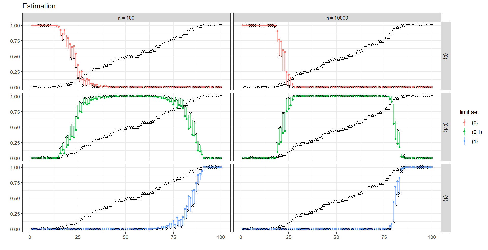
Figure 1. Model parameters: $N=3$, $r_{n}=\frac{c}{(0.1+n)^{\gamma}}$ with $c=1$ and $\gamma=0.75$, the interaction matrix $W$ is of the mean-field type, precisely $w_{l_{1},l_{2}}=\frac{1}{2N}+\frac{1}{2}\delta_{l_{1},l_{2}}$, with initial condition ${\boldsymbol{Z}}_{0}=\frac{1}{2}{\boldsymbol{1}}$. Number of simulations $S=10^{2}$.
Parameters for the estimating procedure: $K=10^{2}$, $n=10^{2},10^{4}$ and $t=n+10^{4}$ (that satisfies the guidelines of Section B of the Appendix, e.g. with $\eta=0.2$ and $\epsilon=0.05$). In each panel identified by $n$ and a limit set $z=\{0\},(0,1),\{1\}$, the triangles correspond to the values of $\widetilde{Z}_{n}$ for the different $S$ simulations. The circular dots represent the estimate $U^{\prime K}_{z,n,t}$ for the different $S$ simulations. The crosses represent the target values $P_{z,n}\stackrel{{\scriptstyle a.s.}}{{=}}\lim_{K,t\rightarrow+\infty}U^{\prime K}_{z,n,t}$, here estimated as $U^{\prime K}_{z,n,10^{5}}$, for the different $S$ simulations. The vertical segments indicate the differences between the estimates and the corresponding target values.

Notice in Figure 1 how the estimates change according to the values of $\widetilde{Z}_{n}$ observed in the different simulations: when $\widetilde{Z}_{n}$ is very close to a barrier, $z=0$ or $z=1$, then the corresponding $U^{\prime K}_{z,n,t}$ is close to one as well, while when $\widetilde{Z}_{n}$ lies within (0,1) and is far from the barriers, then both $U^{\prime K}_{0,n,t}$ and $U^{\prime K}_{1,n,t}$ are very small, so leading $U^{\prime K}_{(0,1),n,t}$ to be large instead. In addition, notice how the estimates of $U^{\prime K}_{z,n,t}$ get more extreme with a larger value of $n$, since the probability of polarization itself gets close to 1 or 0 with more observations, i.e. $U^{\prime K}_{z,n,t}\stackrel{{\scriptstyle a.s.}}{{\longrightarrow}}_{t,K}P_{z,n}\stackrel{{\scriptstyle a.s.}}{{\longrightarrow}}_{n}I_{z}(Z_{\infty})\in\{0,1\}$.

Figure 2 is focused on the construction of a confidence interval for $Z_{\infty}$ in the same framework as considered in Figure 1. In particular, it shows how the asymptotic confidence interval $I^{K}_{n,t,1-\alpha}$ presented in Section 5 can be composed by different disjoint sets: $\{0\}$, $\{1\}$ and $I^{K}_{(0,1),n,t,\theta}$, i.e. the two barriers and the interval for the case $0<Z_{\infty}<1$. The specific form assumed by the interval depends on the observation of the system until the time-step $n$, and in particular on $\widetilde{Z}_{n}$. Indeed, from Figure 2 it is evident that when $\widetilde{Z}_{n}$ is very close to a barrier, $z=0$ or $z=1$, the interval is only made by that barrier $z$, while when $\widetilde{Z}_{n}$ remains inside $(0,1)$ and is far from the barriers we get a more classical two-sided interval that excludes them. Naturally, with a larger value of $n$ we observe more intervals composed by a single set, which can be $\{0\}$, $\{1\}$ or the interval $I^{K}_{(0,1),n,t,\theta}$, that gets narrower as a natural consequence of the fact that $\widetilde{Z}_{n}\stackrel{{\scriptstyle a.s.}}{{\longrightarrow}}Z_{\infty}$.

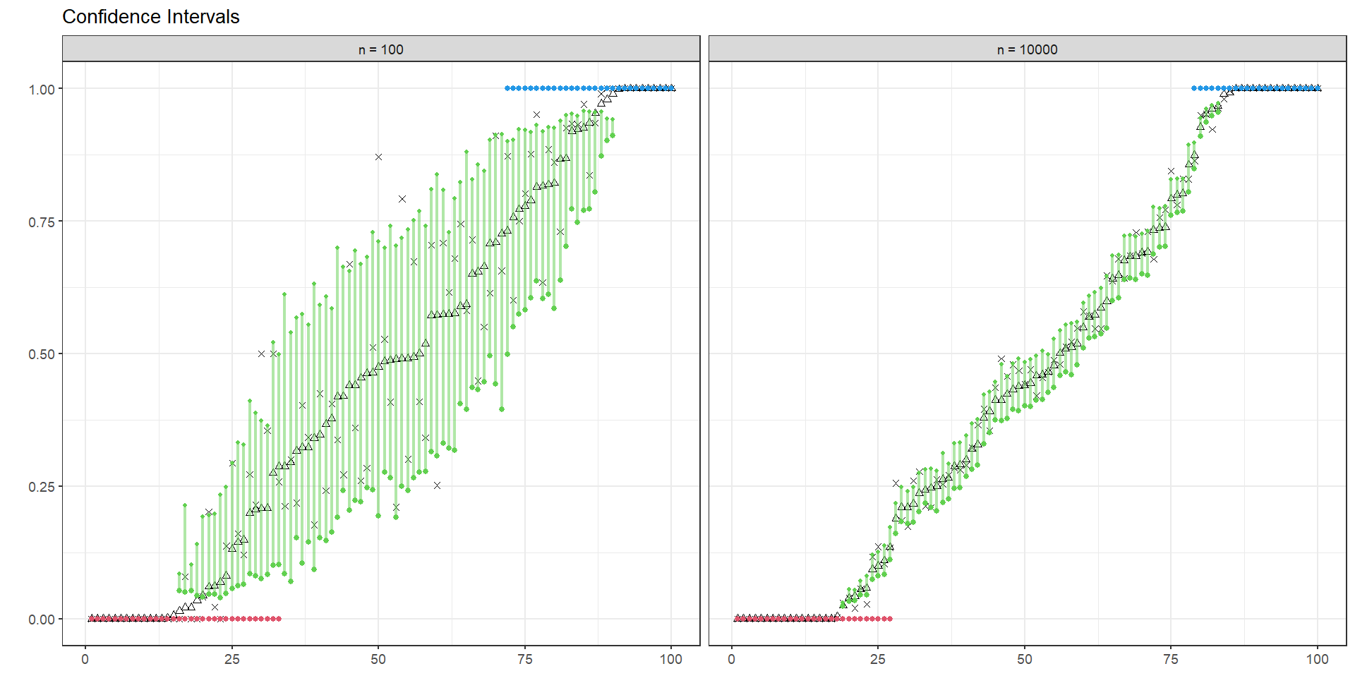
Figure 2. Model parameters: $N=3$, $r_{n}=\frac{c}{(0.1+n)^{\gamma}}$ with $c=1$ and $\gamma=0.75$, the interaction matrix $W$ is of the mean-field type, precisely $w_{l_{1},l_{2}}=\frac{1}{2N}+\frac{1}{2}\delta_{l_{1},l_{2}}$, with initial condition ${\boldsymbol{Z}}_{0}=\frac{1}{2}{\boldsymbol{1}}$. Number of simulations $S=10^{2}$.
Parameters for the estimating procedure: $K=10^{2}$, $n=10^{2},10^{4}$, $t=n+10^{4}$ (that satisfies the guidelines of Section B of the Appendix, e.g. with $\eta=0.2$ and $\epsilon=0.05$) and confidence level $1-\alpha=0.95$. In each panel identified by $n$, the (possible) three parts that can compose the confidence interval $I^{K}_{n,t,1-\alpha}$ are reported: the set $\{0\}$ (red), the set $\{1\}$ (blue) and the interval $I^{K}_{(0,1),n,t,\theta}$ (green). The triangles correspond to the values of $\widetilde{Z}_{n}$ for the different $S$ simulations. The crosses represent the target values $Z_{\infty}\stackrel{{\scriptstyle a.s.}}{{=}}\lim_{t\rightarrow+\infty}\widetilde{Z}_{t}$, here estimated as $\widetilde{Z}_{10^{5}}$, for the different $S$ simulations.

Remark 9.

We observe that the estimating procedure for the probability of asymptotic polarization and the construction of the asymptotic confidence interval for $Z_{\infty}$ can be adapted to the case when only the asymptotic behaviour of $(r_{n})$ is known and the observable variables are the agents’ actions $X_{n,\ell}$. In that case, we have to replace the random variables $Z_{n,\ell}$ by the empirical means $\sum_{k=1}^{n}X_{k,\ell}/n$ or by suitable weighted empirical means [3, 4].

Declaration
All the authors contributed equally to the present work.

Funding Sources
Irene Crimaldi is partially supported by the Italian “Programma di Attività Integrata” (PAI), project “TOol for Fighting FakEs” (TOFFE) funded by IMT School for Advanced Studies Lucca. Giacomo Aletti and Irene Crimaldi are partially supported by the project “Optimal and adaptive designs for modern medical experimentation” funded by the Italian Government (MIUR, PRIN 2022).

Acknowledgements
The authors thank the referees for carefully reading the manuscript and for their suggestions to improve it.

Appendix A Some auxiliary results

We start with the proof of Lemma 2.3.

Proof of Lemma 2.3.

a) In order to prove (11), we note that

$$\sum_{n\geq 0}\frac{r_{n}}{\sum_{k=0}^{n}r_{k}}=1+\sum_{n\geq 1}\frac{r_{n}}{\sum_{k=0}^{n}r_{k}}$$

and, since $\sum_{k=0}^{n-1}r_{k}/\sum_{k=0}^{n}r_{k}=(1+r_{n}/\sum_{k=0}^{n-1}r_{k})^{-1}\to 1$ when $\sum_{n}r_{n}=+\infty$, we have that the series $\sum_{n\geq 1}\frac{r_{n}}{\sum_{k=0}^{n}r_{k}}$ has the same behaviour as the series $\sum_{n\geq 1}\frac{r_{n}}{\sum_{k=0}^{n-1}r_{k}}$ (i.e. they are both convergent or both divergent). In order to prove that the last series diverges to $+\infty$, we observe that

$$\sum_{n\geq 1}\frac{r_{n}}{\sum_{k=0}^{n-1}r_{k}}=\sum_{n\geq 1}\int_{\sum_{k=0}^{n-1}r_{k}}^{\sum_{k=0}^{n}r_{k}}\frac{1}{\sum_{k=0}^{n-1}r_{k}}dx\geq\sum_{n\geq 1}\int_{\sum_{k=0}^{n-1}r_{k}}^{\sum_{k=0}^{n}r_{k}}\frac{1}{x}dx=\int_{r_{0}}^{+\infty}\frac{1}{x}\,dx=+\infty.$$

b) The relation (12) follows by combining the following inequalities:

(23) $$\begin{split}\sum_{k=0}^{n}r_{k}&=\sum_{k=0}^{n}\frac{\alpha_{k+1}}{s_{k+1}}=\sum_{k=0}^{n}\int_{s_{k}}^{s_{k+1}}\frac{1}{s_{k+1}}\,dx\\ &\leq\sum_{k=0}^{n}\int_{s_{k}}^{s_{k+1}}\frac{1}{x}\,dx=\int_{s_{0}}^{s_{n+1}}\frac{1}{x}\,dx=\ln(s_{n+1})-\ln(s_{0})\leq\ln(s_{n+1})\end{split}$$

and

(24) $$\begin{split}\frac{1}{1-\sup_{n}r_{n}}\sum_{k=0}^{n}r_{k}&\geq\sum_{k=0}^{n}\frac{r_{k}}{1-r_{k}}=\sum_{k=0}^{n}\frac{\alpha_{k+1}}{s_{k}}=\sum_{k=0}^{n}\int_{s_{k}}^{s_{k+1}}\frac{1}{s_{k}}\,dx\\ &\geq\sum_{k=0}^{n}\int_{s_{k}}^{s_{k+1}}\frac{1}{x}\,dx=\int_{s_{0}}^{s_{n+1}}\frac{1}{x}\,dx=\ln(s_{n+1})-\ln(s_{0}).\end{split}$$

Indeed, we get

(25) $$(1-\sup_{n}r_{n})\left(1-\frac{\ln(s_{0})}{\ln(s_{n+1})}\right)\leq\frac{\sum_{k=0}^{n}r_{k}}{\ln(s_{n+1})}\leq 1$$

and, since the limit of $\ln(s_{0})/\ln(s_{n+1})$ is strictly smaller than $1$ if $\sup_{n}r_{n}>0$ (i.e. if the numbers $\alpha_{n}$ are not all equal to zero), there exists a real constant $c>0$ such that

$$c\leq\liminf_{n}\frac{\sum_{k=0}^{n}r_{k}}{\ln(s_{n+1})}\leq\limsup_{n}\frac{\sum_{k=0}^{n}r_{k}}{\ln(s_{n+1})}\leq 1\,.$$

c) It is immediate to see that (13) implies (10) since $(1-x)\leq e^{-x}$ $\forall x>0$. The converse is also trivial when $\sum_{n}r_{n}<+\infty$. Indeed, (10) is always verified when $\sum_{n}r_{n}<+\infty$ and $\sum_{n}r_{n}<+\infty$ trivially implies $\sum_{n}r_{n}^{2}<+\infty$ since $r_{n}<1$ $\forall n$.
Now, we focus on the case when $\sum_{n}r_{n}=+\infty$. In that case, there exists $N>0$ such that $\sum_{k=0}^{N-1}r_{k}\geq 1$. Then, since $x\mapsto xe^{-x}$ is decreasing on $[1,\infty)$, under (10) we obtain

$$\sum_{n\geq N}r_{n}^{2} \leq\sum_{n\geq N}r_{n}\Big{(}Ce^{-\sum_{k=0}^{n}r_{k}}\sum_{k=0}^{n}r_{k}\Big{)}=C\sum_{n\geq N}\int_{\sum_{k=0}^{n-1}r_{k}}^{\sum_{k=0}^{n}r_{k}}e^{-\sum_{k=0}^{n}r_{k}}\sum_{k=0}^{n}r_{k}dx$$

$$\leq C\sum_{n\geq N}\int_{\sum_{k=0}^{n-1}r_{k}}^{\sum_{k=0}^{n}r_{k}}e^{-x}xdx\leq C\int_{1}^{+\infty}e^{-x}xdx<+\infty,$$

and so the first part of point c) is proven, that is (10) implies $\sum_{n}r_{n}^{2}<+\infty$ (and so $r_{n}\to 0$). As a consequence of this first result, we have

$$\sum_{k=0}^{n}\frac{r_{k}}{1-r_{k}}-\sum_{k=0}^{n}r_{k}=\sum_{k=0}^{n}\frac{r_{k}^{2}}{1-r_{k}}<+\infty\,.$$

Therefore, using the inequality (24) for $\sum_{k=0}^{n}\frac{r_{k}}{1-r_{k}}$, we obtain

$$\sum_{k=0}^{n}r_{k}\geq\ln(s_{n+1})-\ln(s_{0})-\sum_{k=0}^{n}\frac{r_{k}^{2}}{1-r_{k}}\,,$$

that is $s_{n+1}=O\left(\exp(\sum_{k=0}^{n}r_{k})\right)$. Then, (10) also implies (13): indeed, for suitable real constants $C_{1}>0$ and $C_{2}>0$, we have

$$\frac{r_{n}}{\prod_{k=0}^{n}(1-r_{k})} =r_{n}\frac{s_{n+1}}{s_{0}}$$

$$\leq\Big{(}C_{1}e^{-\sum_{k=0}^{n}r_{k}}\sum\nolimits_{k=0}^{n}r_{k}\Big{)}(C_{2}e^{\sum_{k=0}^{n}r_{k}})\leq C_{1}C_{2}\sum\nolimits_{k=0}^{n}r_{k}.$$

Recalling that $\alpha_{n+1}=s_{0}\frac{r_{n}}{\prod_{k=0}^{n}(1-r_{k})}$ and using (25), we get that (13) is equivalent to (14), i.e. $\alpha_{n+1}=O(\ln(s_{n+1}))$. Finally, recalling that $s_{n+1}=s_{0}/\prod_{k=0}^{n}(1-r_{k})$ and using (25), we also obtain that (13) is equivalent to (15), i.e. $r_{n}=O(\ln(s_{n+1})/s_{n+1})$. ∎

For reader’s convenience, we here recall some general results. In particular, the first one is a little generalization of [2, Lemma A.4].

Lemma A.1.

Given $1/2<\gamma\leq 1$ and $c>0$, let $(r_{n})_{n}$ be a sequence of real numbers such that $0\leq r_{n}<1$,

$$\lim_{n}n^{\gamma}r_{n}=c\quad\mbox{ and }\quad\sum_{n}(r_{n}-cn^{-\gamma})\;\mbox{ is convergent}\,.$$

Then we have

$$\prod_{k=0}^{n}(1-r_{k})\ =\ \begin{cases}O\left(\exp\left[-\frac{c}{1-\gamma}n^{1-\gamma}\right]\right)&\mbox{for }1/2<\gamma<1,\\ O\left(n^{-c}\right)&\mbox{for }\gamma=1\,.\end{cases}$$

We omit the proof of the above lemma because it is exactly the same as the one of [2, Lemma A.4].

Theorem A.2 ([15, Theorem 46, p. 40]).

Let $(Y_{n})_{n}$ be a sequence of positive (i.e. non-negative) random variables, adapted to a filtration $\mathcal{G}$. Then the set $\{\sum_{n}E[Y_{n+1}|\mathcal{G}_{n}]<+\infty\}$ is almost surely contained in the set $\{\sum_{n}Y_{n}<+\infty\}$. If the random variables $Y_{n}$ are uniformly bounded by a constant, then these two sets are almost surely equal.

Appendix B Practical guidelines on the choice of the time $t$

In this section we provide a practical guideline on the choice of the time-step $t>n$ that has to be used in the above described estimating procedure.
For instance, consider the estimator $U^{\prime K}_{0,n,t}=\frac{1}{K}\sum_{j=1}^{K}U^{j}_{0,t}$ of $P_{0,t}$ (analogous arguments can be made for the estimator $U^{\prime K}_{1,n,t}$ of $P_{1,t}$) and focus on a single realization $U^{j}_{0,t}$ and, in particular, on its expression in (22), where it is defined as a function of the ratio $\sum_{k=t}^{\infty}r_{k}^{2}/(M_{t}^{j})^{2}$. Since by Proposition 4.1 $U^{j}_{0,t}\stackrel{{\scriptstyle a.s.}}{{\longrightarrow}}_{t}I_{0}(M^{j}_{\infty})$, this ratio must tend to infinity a.s. on the set $\{M^{j}_{\infty}=0\}$. On the other hand, since $\sum_{n}r_{n}^{2}<+\infty$, we obviously have that it tends to zero a.s. on the set $\{0<M^{j}_{\infty}\leq 1\}$. Moreover, we notice that $(M_{t}^{j})^{2}$ is bounded by $1$, while $\sum_{k=t}^{\infty}r_{k}^{2}$, although it always tends to zero, can be very large for small $t$ (much larger than $1$). As a consequence, if $U^{j}_{0,t}$ is computed when the time-step $t$ is small, the ratio $\sum_{k=t}^{\infty}r_{k}^{2}/(M_{n}^{j})^{2}$ (and so $U^{j}_{0,t}$) may be always large, regardless of the value of $M^{j}_{t}$, i.e. regardless of the information contained in $\mathcal{G}_{n}$ used to generate $M^{j}_{t}$. To address this issue, we can impose some initial conditions in order to ensure that:

• $U^{j}_{0,t}$ is small when $M^{j}_{t}$ is not very close to $0$;

• $U^{j}_{1,t}$ is small when $M^{j}_{t}$ is not very close to $1$.

Formally, we can fix $\epsilon>0$ and $\eta>0$ such that $U^{j}_{0,t}<\epsilon$ when $M^{j}_{t}>\eta$ and, analogously, $U^{j}_{1,t}<\epsilon$ when $M^{j}_{t}<1-\eta$. These constraints provide us with a condition on the minimum time-step $t_{\min}$ that we should take to compute the previous estimators: indeed, we have that $t_{\min}$ should be the minimum integer $t$ such that

$$\exp\left(-2\frac{\eta^{2}}{\sum_{k=t}^{\infty}r_{k}^{2}}\right)<\epsilon,\ \mbox{that is}\ \sum_{k=t}^{\infty}r_{k}^{2}<\frac{2\eta^{2}}{\ln\left(\frac{1}{\epsilon}\right)}.$$

Appendix C Periodicity of a matrix

Let $A$ be a non-negative $N\times N$ square matrix such that $A^{\top}{\boldsymbol{1}}={\boldsymbol{1}}$. Then, for any element $l\in V=\{1,\dots,N\}$, we can define the period of $l$, say $d(l)$, as the greatest common divisor $n\in\mathbb{N}$ such that $A^{n}_{l,l}>0$. Then, if $A$ is also irreducible, all the elements will have the same period and so we can define the period of the matrix $A$ as $d=d(1)=\dots=d(N)$. A matrix with period $d=1$ is called aperiodic, otherwise a matrix with period $d\geq 2$ is called periodic.

References

- [1] R. Albert and A.-L. Barabási. Statistical mechanics of complex networks. Rev. Modern Phys., 74(1):47–97, 2002.
- [2] G. Aletti, I. Crimaldi, and A. Ghiglietti. Synchronization of reinforced stochastic processes with a network-based interaction. Ann. Appl. Probab., 27(6):3787 ? 3844, 2017.
- [3] G. Aletti, I. Crimaldi, and A. Ghiglietti. Networks of reinforced stochastic processes: asymptotics for the empirical means. Bernoulli, 25(4 B):3339–3378, 2019.
- [4] G. Aletti, I. Crimaldi, and A. Ghiglietti. Interacting reinforced stochastic processes: Statistical inference based on the weighted empirical means. Bernoulli, 26(2):1098–1138, 2020.
- [5] G. Aletti, I. Crimaldi, and A. Ghiglietti. Networks of reinforced stochastic processes: a complete description of the first-order asymptotics. arXiv:2206.07514, 2022.
- [6] G. Aletti and A. Ghiglietti. Interacting generalized Friedman’s urn systems. Stoch. Process. Appl., 127(8):2650–2678, 2017.
- [7] A. Arenas, A. Díaz-Guilera, J. Kurths, Y. Moreno, and C. Zhou. Synchronization in complex networks. Phys. Rep., 469(3):93–153, 2008.
- [8] M. Benaïm, I. Benjamini, J. Chen, and Y. Lima. A generalized Pólya’s urn with graph based interactions. Random Struct. Algor., 46(4):614–634, 2015.
- [9] D. Blackwell and L. Dubins. Merging of opinions with increasing information. Ann. Math. Statist., 33:882–886, 1962.
- [10] S. Boucheron, G. Lugosi, and P. Massart. Concentration inequalities. Oxford University Press, Oxford, 2013.
- [11] J. Chen and C. Lucas. A generalized Pólya’s urn with graph based interactions: convergence at linearity. Electron. Commun. Probab., 19:no. 67, 13, 2014.
- [12] I. Crimaldi. An almost sure conditional convergence result and an application to a generalized Pólya urn. Int. Math. Forum, 4(21-24):1139–1156, 2009.
- [13] I. Crimaldi, P. Dai Pra, P.-Y. Louis, and I. G. Minelli. Synchronization and functional central limit theorems for interacting reinforced random walks. Stoch. Process. Appl., 129(1):70–101, 2019.
- [14] I. Crimaldi, P.-Y. Louis, and I. G. Minelli. Interacting non-linear reinforced stochastic processes: synchronization or non-synchronization. Adv. in Appl. Probab., 55(1):forthcoming, 2023.
- [15] C. Dellacherie and P.-A. Meyer. Probabilities and Potential. B, volume 72 of North-Holland Mathematics Studies. North-Holland Publishing Co., Amsterdam, 1982.
- [16] D. Freedman. Another note on the Borel-Cantelli lemma and the strong law, with the Poisson approximation as a by-product. Ann. Probability, 1:910–925, 1973.
- [17] M. Hayhoe, F. Alajaji, and B. Gharesifard. A Polya contagion model for networks. IEEE Trans. Control Netw. Syst., 5(4):1998–2010, 2018.
- [18] G. Kaur and N. Sahasrabudhe. Interacting urns on a finite directed graph. J. Appl. Probab., page Forthcoming, 2022.
- [19] D. Lamberton, G. Pagès, and P. Tarrès. When can the two-armed bandit algorithm be trusted? Ann. Appl. Probab., 14(3):1424–1454, 2004.
- [20] Y. Lima. Graph-based Pólya’s urn: completion of the linear case. Stoch. Dyn., 16(2):1660007, 13, 2016.
- [21] M. E. J. Newman. Networks: An introduction. Oxford University Press, Oxford, 2010.
- [22] R. Pemantle. A time-dependent version of Pólya’s urn. J. Theoret. Probab., 3(4):627–637, 1990.
- [23] N. Sahasrabudhe. Synchronization and fluctuation theorems for interacting Friedman urns. J. Appl. Probab., 53(4):1221–1239, 2016.
- [24] N. Sidorova. Time-dependent Pólya urn, 2018.
- [25] R. van der Hofstad. Random graphs and complex networks. Vol. 1. Cambridge Series in Statistical and Probabilistic Mathematics, [43]. Cambridge University Press, Cambridge, 2017.