Fast and exact fixed-radius neighbor search based on sorting

Abstract

Fixed-radius near neighbor search is a fundamental data operation that retrieves all data points within a user-specified distance to a query point. There are efficient algorithms that can provide fast approximate query responses, but they often have a very compute-intensive indexing phase and require careful parameter tuning. Therefore, exact brute force and tree-based search methods are still widely used. Here we propose a new fixed-radius near neighbor search method, called SNN, that significantly improves over brute force and tree-based methods in terms of index and query time, provably returns exact results, and requires no parameter tuning. SNN exploits a sorting of the data points by their first principal component to prune the query search space. Further speedup is gained from an efficient implementation using high-level Basic Linear Algebra Subprograms (BLAS). We provide theoretical analysis of our method and demonstrate its practical performance when used stand-alone and when applied within the DBSCAN clustering algorithm.

1 Introduction

This work is concerned with the retrieval of nearest neighbors, a fundamental data operation. Given a data point, this operation aims at finding the most similar data points using a predefined distance function. Nearest neighbor search has many applications in computer science and machine learning, including object recognition (Philbin et al.,, 2007; Nister and Stewenius,, 2006), image descriptor matching Silpa-Anan and Hartley, (2008), time series indexing (Keogh and Ratanamahatana,, 2005; Chakrabarti et al.,, 2002; Yagoubi et al.,, 2020), clustering (Ester et al.,, 1996; Campello et al.,, 2013; Gallego et al.,, 2018; Alshammari et al.,, 2021; Gallego et al.,, 2022; Li et al.,, 2020), particle simulations (Groß et al.,, 2019), molecular modeling (Galvelis and Sugita,, 2017), pose estimation (Shakhnarovich et al.,, 2003), computational linguistics (Kaminska et al.,, 2021), and information retrieval (Geng et al.,, 2008; Wang et al.,, 2015).

There are two main types of nearest neighbor (NN) search: $k$-nearest neighbor and fixed-radius near neighbor search. Fixed-radius NN search, also referred to as radius query, aims at identifying all data points within a given distance from a query point; see Bentley, 1975b for a historical review. The most straightforward way of finding nearest neighbors is via a linear search through the whole database, also known as exhaustive or brute force search. Though considered inelegant, it is still widely used, e.g., in combination with GPU acceleration (Garcia et al.,, 2008).

Existing NN search approaches can be broadly divided into exact and approximate methods. In many applications, approximate methods are an effective solution for performing fast queries while allowing for a small loss. Well-established approximate NN search techniques include randomized $k$-d trees (Silpa-Anan and Hartley,, 2008), hierarchical k-means (Nister and Stewenius,, 2006), locality sensitive hashing (Indyk and Motwani,, 1998), HNSW (Malkov and Yashunin,, 2020), and ScaNN (Guo et al.,, 2020). Considerable drawbacks of most approximate NN search algorithms are their potentially long indexing time and the need for the tuning of additional hyperparameters such as the trade-off between recall versus index and query time. Furthermore, to the best of our knowledge, all approximate NN methods for which open-source implementations (such as those in the footnote) are available only address the k-nearest neighbor problem, not the fixed-radius problem discussed here.

In this paper we introduce a new exact approach to fixed-radius NN search based on sorting, referred to as SNN for short. Some of the appealing properties of SNN are

1. simplicity: SNN has no hyperparameters except for the necessary search radius

2. exactness: SNN is guaranteed to return all data points within the search radius

3. speed: SNN demonstrably outperforms other exact NN search algorithms like, e.g., methods based on tree structures

4. flexibility: the low indexing time of SNN makes it applicable in an online streaming setting.

The rest of this paper is organized as follows. In section 2, we provide a brief review of existing work on NN search. In section 3, we introduce our sorting-based NN method, detailing its indexing and query phases. Section 4 contains computational considerations regarding the efficient implementation of SNN and its behavior in floating-point arithmetic. Theoretical performance analysis is provided in Section 5. Section 6 contains performance comparisons of our algorithm to other state-of-the-art NN methods, as well as an application to DBSCAN clustering. We then conclude in section 7.

2 Related work

NN search methods can broadly be classified into approximate or exact methods, depending on whether they return exact or approximate answers to queries (Cayton and Dasgupta,, 2007). It is widely accepted that for high-dimensional data there are no exact NN search methods which are asymptotically more efficient than exhaustive search; see, e.g., (Muja,, 2013, Chap. 3) and (Francis-Landau and Durme,, 2019). Exact NN methods based on $k$-d tree (Bentley, 1975a, ; Friedman et al.,, 1977), balltree (Omohundro,, 1989), VP-tree (Yianilos,, 1993), cover tree (Beygelzimer et al.,, 2006), and RP tree (Dasgupta and Sinha,, 2013) only perform well on low-dimensional data. This shortcoming is often referred to as the curse of dimensionality (Indyk and Motwani,, 1998). However, note that negative asymptotic results do not rule out the possibility of algorithms and implementations that perform significantly (by orders of magnitude) faster than brute force search in practice, even on real-world high-dimensional data sets.

To speedup NN search, modern approaches generally focus on two aspects, namely indexing and sketching. The indexing aims to construct a data structure that prunes the search space for a given query, hopefully resulting in fewer distance computations. Sketching, on the other hand, aims at reducing the cost of each distance computation by using a compressed approximate representation of the data.

The most widely used indexing strategy is space partitioning. Some of the earliest approaches are based on tree structures such as $k$-d tree (Bentley, 1975a, ; Friedman et al.,, 1977), balltree (Omohundro,, 1989), VP-tree (Yianilos,, 1993), and cover tree (Beygelzimer et al.,, 2006). The tree-based methods are known to become inefficient for high-dimensional data. One of the remedies are randomization (e.g., (Dasgupta and Sinha,, 2013; Ram and Sinha,, 2019)) and ensembling (e.g., the FLANN nearest neighbor search tool by Muja and Lowe, (2009), which empirically shows competitive performance against approximate NN methods). Another popular space partitioning method is locality-sensitive hashing (LSH); see, e.g., (Indyk and Motwani,, 1998). LSH leverages a set of hash functions from the locality-sensitive hash family and it guarantees that similar queries are hashed into the same buckets with higher probability than less similar ones. This method was originally introduced for the binary Hamming space by Indyk and Motwani, (1998), and it was later extended to the Euclidean space (Datar et al.,, 2004). In (Bawa et al.,, 2005) a self-tuning index for LSH based similarity search was introduced. A partitioning approach based on neural networks and LSH was proposed in Dong et al., (2020). Another interesting method is GriSPy (Chalela et al.,, 2021), which performs fixed-radius NN search using regular grid search—to construct a regular grid for the index—with the possibility of working with periodic boundary conditions. This method, however, has high memory demand because the grid computations grow exponentially with the space dimension.

This paper focuses on exact fixed-radius NN search. The implementations available in the most widely used scientific computing environments are all based on tree structures, including findNeighborsInRadius in MATLAB (The MathWorks Inc.,, 2022), NearestNeighbors in scikit-learn (Pedregosa et al.,, 2011), and spatial in SciPy (Virtanen et al.,, 2020). This is in contrast to our SNN method introduced below which does not utilise any tree structures.

3 Sorting-based NN search

Suppose we have $n$ data points $p_{1},\ldots,p_{n}\in\mathbb{R}^{d}$ (represented as column vectors) and $d\ll n$. The fixed-radius NN problem consists of finding the subset of data points that is closest to a given query point $q\in\mathbb{R}^{d}$ (may be out-of-sample) with respect to some distance metric. Throughout this paper, the vector norm $\|\cdot\|=\|\cdot\|_{2}$ is the Euclidean one, though it also possible to identify nearest neighbors with other distances such as

• cosine distance: assuming normalized data (with $\|u\|=\|v\|=1$), the cosine distance is

  $$\text{cdist}(u,v)=1-\cos(\theta)=1-\frac{u^{T}v}{\|u\|\|v\|}=1-u^{T}v\in[0,2].$$

  Hence, the cosine distance can be computed from the Euclidean distance via

  $$2\text{cdist}(u,v)=2-2u^{T}v=u^{T}u-2u^{T}v+v^{T}v=\|u-v\|^{2}.$$

• angular distance: the angular distance $\theta\in[0,\pi]$ between two normalized vectors $u,v$ satisfies

  $$\theta\leq\alpha\quad\text{if and only if}\quad||u-v||^{2}\leq 2-2\cos(\alpha).$$

  Therefore, closest angle neighbors can be identified via Euclidean distance.

• maximum inner product similarity (see, e.g., Bachrach et al., (2014)): for not necessarily normalized vectors we can consider the transformed data points $\tilde{p}_{i}=[\sqrt{\xi^{2}-\|p_{i}\|^{2}},p_{i}^{T}]^{T}$ with $\xi:=\max_{i}{\|p_{i}\|}$ and the transformed query point $\tilde{q}=[0,q^{T}]^{T}$. Then

  $$\|\tilde{p}_{i}-q\|^{2}=\|\tilde{p}_{i}\|^{2}+\|\tilde{q}\|^{2}-2\tilde{p}_{i}^{T}\tilde{q}=\xi^{2}+\|q\|^{2}-2p_{i}^{T}q\geq 0.$$

  Since $\xi$ and $q$ are independent of the index $i$, we have $\operatorname*{argmin}_{i}\|\tilde{p}_{i}-\tilde{q}\|^{2}=\operatorname*{argmax}_{i}p_{i}^{T}q$.

• Manhattan distance: since $\|p_{i}-q\|_{2}\leq\|p_{i}-q\|_{1}$, any points satisfying $\|p_{i}-q\|_{1}>R$ must necessarily satisfy $\|p_{i}-q\|_{2}>R$. Hence, the sorting-based exclusion criterion proposed in section 3.2 to prune the query search space can also be used for the Manhattan distance.

Our algorithm, called SNN, will return the required indices of the nearest neighbors in the Euclidean norm, and can also return the corresponding distances if needed. SNN uses three essential ingredients to obtain its speed. First, a sorting-based exclusion criterion is used to prune the search space for a given query. Second, pre-calculated dot products of the data points allow for a reduction of arithmetic complexity. Third, a reformulation of the distance criterion in terms of matrices (instead of vectors) allows for the use of high-level basic linear algebra subprograms (BLAS, Blackford et al., (2002)). In the following, we explain these ingredients in more detail.

3.1 Indexing

Before sorting the data, all data points are centered by subtracting the empirical mean value of each dimension:

$$x_{i}:=p_{i}-\mathrm{mean}(\{p_{j}\}).$$

This operation will not affect the pairwise Euclidean distance between the data points and can be performed in $O(dn)$ operations, i.e. with linear complexity in $n$. We then compute the first principal component $v_{1}\in\mathbb{R}^{d}$, i.e., the vector along which the data $\{x_{i}\}$ exhibits largest empirical variance. This vector can be computed by a thin singular value decomposition of the tall-skinny data matrix $X:=[x_{1},\ldots,x_{n}]^{T}\in\mathbb{R}^{n\times d}$,

$$X=U\Sigma V^{T},$$ (1)

where $U\in\mathbb{R}^{n\times d}$ and $V\in\mathbb{R}^{d\times d}$ have orthonormal columns and $\Sigma=\mathrm{diag}(\sigma_{1},\ldots,\sigma_{d})\in\mathbb{R}^{d\times d}$ is a diagonal matrix such that $\sigma_{1}\geq\sigma_{2}\geq\cdots\geq\sigma_{d}\geq 0.$ The principal components are given as the columns of $V=[v_{1},\ldots,v_{d}]$ and we require only the first column $v_{1}$. The score of a point $x_{i}$ along $v_{1}$ is

$$\alpha_{i}:=x_{i}^{T}v_{1}=(e_{i}^{T}X)v_{1}=(e_{i}^{T}U\Sigma V^{T})v_{1}=e_{i}^{T}u_{1}\sigma_{1},$$

where $e_{i}$ denotes the $i$-th canonical unit vector in $\mathbb{R}^{n}$. In other words, the scores $\alpha_{i}$ of all points can be read off from the first column of $U=[u_{1},\ldots,u_{d}]$ times $\sigma_{1}$. The computation of the scores using a thin SVD requires $O(nd^{2})$ operations and is therefore linear in $n$.

The next (and most important) step is to order all data points $x_{i}$ by their $\alpha_{i}$ scores; that is,

$$(x_{i}):=\mathrm{sort}(\{x_{i}\})$$

so that $\alpha_{1}\leq\alpha_{2}\leq\cdots\leq\alpha_{n}$ with each $\alpha_{i}=x_{i}^{T}v_{1}$. This sorting will generally require a time complexity of $O(n\log n)$ independent of the data dimension $d$. We also precompute the squared-and-halved norm of each data point, $\overline{x_{i}}=(x_{i}^{T}x_{i})/2$ for $i=1,2,\ldots,n$. This is of complexity $O(nd)$, i.e., again linear in $n$.

All these computations are done exactly once in the indexing phase and only the scores $[\alpha_{i}]$, the numbers $[\overline{x_{i}}]$, and the single vector $v_{1}$ need to be stored. See Algorithm 1 for a summary.

Algorithm 1 SNN Index

1:Input: Data matrix $P=[p_{1},p_{2},\ldots,p_{n}]^{T}\in\mathbb{R}^{n\times d}$

2:Compute $\mu:=\mathrm{mean}(\{p_{j}\})$

3:Compute the mean-centered matrix $X$ with rows $x_{i}:=p_{i}-\mu$

4:Compute the singular value decomposition of $X=U\Sigma V^{T}$

5:Compute the sorting keys $\alpha_{i}=x_{i}^{T}v_{1}$ for $i=1,2,\ldots,n$

6:Sort data points $X$ such that $\alpha_{1}\leq\alpha_{2}\leq\cdots\leq\alpha_{n}$

7:Compute $\overline{x_{i}}=(x_{i}^{T}x_{i})/2$ for $i=1,2,\ldots,n$

8:Return: $\mu$, $X$, $v_{1}$, $[\alpha_{i}]$, $[\overline{x_{i}}]$

3.2 Query

Given a query point $q$ and user-specified search radius $R$, we want to retrieve all data points $p_{i}$ satisfying $\|p_{i}-q\|\leq R$. Figure 1 illustrates our approach. We first compute the mean-centered query $x_{q}:=q-\mathrm{mean}(\{p_{j}\})$ and the corresponding score $\alpha_{q}:=x_{q}^{T}v_{1}$. By utilizing the Cauchy–Schwarz inequality, we have

$$|\alpha_{i}-\alpha_{q}|=|v_{1}^{T}x_{i}-v_{1}^{T}x_{q}|\leq\|x_{i}-x_{q}\|.$$ (2)

Since we have sorted the $x_{i}$ such that $\alpha_{1}\leq\alpha_{2}\leq\cdots\leq\alpha_{n}$, the following statements are true:

$$\text{if}\ \alpha_{q}-\alpha_{j_{1}}>R\ \text{for some $j_{1}$},\ \text{then}\ \|x_{i}-x_{q}\|>R\ \text{for all $i\leq j_{1}$};$$

$$\text{if}\ \alpha_{j_{2}}-\alpha_{q}>R\ \text{for some $j_{2}$},\ \text{then}\ \|x_{i}-x_{q}\|>R\ \text{for all $i\geq j_{2}$}.$$

As a consequence, we only need to consider candidates $x_{i}$ whose indices are in $J:=\{j_{1}+1,j_{1}+2,\ldots,j_{2}-1\}$ and we can determine the smallest subset by finding the largest $j_{1}$ and smallest $j_{2}$ satisfying the above statements, respectively. As the $\alpha_{i}$ are sorted, this can be achieved via binary search in $O(\log n)$ operations. Note that the indices in $J$ are continuous integers, and hence it is memory efficient to access $X(J,:)$, the submatrix of $X$ whose row indices are in $J$. This will be important later.

Finally, we filter all data points in the reduced set $X(J,:)$, retaining only those data points whose distance to the query point $x_{q}$ is less or equal to $R$, i.e., points satisfying $\|x_{j}-x_{q}\|^{2}\leq R^{2}$. The query phase is summarized in Algorithm 2.

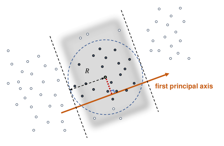
Figure 1: Query with radius $R$. The data points in the shaded band have their first principal coordinate within a distance $R$ from the first principal coordinate of the query point, and hence are NN candidates. All data points are sorted so that all candidates have continuous indices.

4 Computational considerations

The compute-intensive step of the query procedure is the computation of

$$\|x_{j}-x_{q}\|^{2}=(x_{j}-x_{q})^{T}(x_{j}-x_{q})$$ (3)

for all vectors $x_{j}$ with indices $j\in J$. Assuming that these vectors have $d$ features, one evaluation of (3) requires $3d-1$ floating point operations (flop): $d$ flop for the subtractions, $d$ flop for the squaring, and $d-1$ flop for the summation. In total, $|J|(3d-1)$ flop are required to compute all $|J|$ squared distances. We can equivalently rewrite (3) as $\|x_{j}-x_{q}\|^{2}=x_{j}^{T}x_{j}+x_{q}^{T}x_{q}-2x_{j}^{T}x_{q}$ and instead verify the radius condition as

$$\frac{1}{2}x_{j}^{T}x_{j}-x_{j}^{T}x_{q}\leq\frac{R^{2}-x_{q}^{T}x_{q}}{2}.$$ (4)

This form has the advantage that all the squared-and-halved norms $\overline{x_{j}}=(x_{j}^{T}x_{j})/2$ ($i=1,2,\ldots,n$) have been precomputed during the indexing phase. Hence, in the query phase, the left-hand side of (4) can be evaluated for all $|J|$ points $x_{j}$ using only $2d|J|$ flop: $(2d-1)|J|$ for the inner products and $|J|$ subtractions.

Merely counting flop, (4) saves about 1/3 of arithmetic operations over (3). An additional advantage results from the fact that all inner products in (4) can be computed as $X(J,:)^{T}x_{q}$ using level-2 BLAS matrix-vector multiplication (gemv), resulting in further speedup on modern computing architectures. If multiple query points are given, say $x_{q}^{(1)},\ldots,x_{q}^{(\ell)}$, a level-3 BLAS matrix-matrix multiplication (gemm) evaluates $X(J,:)^{T}[x_{q}^{(1)},\ldots,x_{q}^{(\ell)}]$ in one go, where $J$ is the union of candidates for all $\ell$ query points.

One may be concerned that the computation using (4) incurs more rounding error than the usual formula (3). We now prove that this is not the case. First, note that division or multiplication by 2 does not incur rounding error. Using the standard model of floating point arithmetic, we have $fl(a\circ b)=(a\circ b)(1\pm\delta)$ for any elementary operation $\circ\in\{+,-,\times,/\}$, where $0\leq\delta\leq u$ with the unit roundoff $u$ (Higham,, 2002, Chap. 1). Suppose we have two vectors $x$ and $y$ where $x_{i}$ and $y_{i}$ denote their respective coordinates. Then computing

$$s_{d}:=\sum_{i=1}^{d}(x_{i}-y_{i})^{2}=(x-y)^{T}(x-y)$$

in floating point arithmetic amounts to evaluating

$$\widehat{s}_{1} =fl((x_{1}-y_{1})^{2})=fl((x_{1}-y_{1}))^{2}\cdot(1\pm\delta)=(x_{1}-y_{1})^{2}(1\pm\delta)^{3},$$

$$\widehat{s}_{2} =fl(\widehat{s}_{1}+(x_{2}-y_{2})^{2})=(\hat{s}_{1}+(x_{2}-y_{2})^{2}(1\pm\delta)^{3})\cdot(1\pm\delta)$$

$$=(x_{1}-y_{1})^{2}(1\pm\delta)^{4}+(x_{2}-y_{2})^{2}(1\pm\delta)^{4},\ \text{and so on.}$$

Continuing this recursion we arrive at

$$\widehat{s}_{d} =(x_{1}-y_{1})^{2}(1\pm\delta)^{d+2}+(x_{2}-y_{2})^{2}(1\pm\delta)^{d+2}+(x_{3}-y_{3})^{2}(1\pm\delta)^{d+1}$$

$$+\cdots+(x_{d}-y_{d})^{2}(1\pm\delta)^{4}.$$

Assuming $ju<1$ and using (Higham,, 2002, Lemma 3.1) we have

$$(1\pm\delta)^{j}=1+\theta_{j},\ \ \text{where}\ \ |\theta_{j}|\leq\frac{ju}{1-ju}:=\gamma_{j}.$$

Hence,

$$\ \ \ \ \,\,|(x-y)^{T}(x-y)-fl((x-y)^{T}(x-y))|$$

$$\leq|\theta_{d+2}(x_{1}-y_{1})^{2}+\theta_{d+2}^{{}^{\prime}}(x_{2}-y_{2})^{2}+\theta_{d+1}(x_{3}-y_{3})^{2}+$$

$$\cdots+\theta_{4}(x_{d}-y_{d})^{2}|$$

$$\leq|\theta_{d+2}|(x_{1}-y_{1})^{2}+|\theta_{d+2}^{{}^{\prime}}|(x_{2}-y_{2})^{2}+|\theta_{d+1}|(x_{3}-y_{3})^{2}+$$

$$\ldots+|\theta_{4}|(x_{d}-y_{d})^{2}|$$

$$\leq\gamma_{d+2}(x-y)^{T}(x-y),$$

showing that the left-hand side of (3) can be evaluated with high relative accuracy.

A very similar calculation can be done for the formula

$$x^{T}x+y^{T}y-2x^{T}y=s_{d},$$

the expression that is used to derive (4). Using the standard result for inner products (Higham,, 2002, eq. (3.2))

$$fl(x^{T}y) =x_{1}y_{1}(1\pm\delta)^{d}+x_{2}y_{2}(1\pm\delta)^{d}+x_{3}y_{3}(1\pm\delta)^{d-1}$$

$$+\cdots+x_{d}y_{d}(1\pm\delta)^{2},$$

one readily derives

$$|(x-y)^{T}(x-y)-fl(x^{T}x+y^{T}y-2x^{T}y)|\leq\gamma_{d+2}(x-y)^{T}(x-y),$$

the same bound on the relative accuracy of floating-point evaluation as obtained for (3).

Algorithm 2 SNN Query

1:Input: Query vector $q$; user-specified radius $R$; output from Algorithm 1

2:Compute $x_{q}:=q-\mu$

3:Compute the sorting score of $x_{q}$, i.e., $\alpha_{q}:=x_{q}^{T}v_{1}$

4:Select candidate index range $J$ so that $|\alpha_{j}-\alpha_{q}|\leq R$ for all $j\in J$

5:Compute $d:=\overline{x}(J)-X(J,:)^{T}x_{q}$ using the precomputed $\overline{x}=[\overline{x_{i}}]$

6:Return: Points $x_{j}$ with $d_{j}\leq(R^{2}-x_{q}^{T}x_{q})/2$ according to (4)

5 Theoretical analysis

The efficiency of the SNN query in Algorithm 2 is dependent on the number of pairwise distance computations that are performed in Step 5, depending on the size of the index set $|J|$. If the index set $J$ is the full $\{1,2,\ldots,n\}$, then the algorithm reduces to exhaustive search over the whole dataset $\{x_{1},x_{2},\ldots,x_{n}\}$, which is undesirable. For the algorithm to be most efficient, $|J|$ would exactly coincide with the indices of data points $x_{i}$ that satisfy $\|x_{i}-x_{q}\|\leq R$. In practice, the index set $J$ will be somewhere in between these two extremes. Thus, it is natural to ask: How likely is it that $|\alpha_{i}-\alpha_{q}|\leq R$, yet $\|x_{i}-x_{q}\|>R$?

First note that, using the singular value decomposition (1) of the data matrix $X$, we can derive an upper bound on $\|x_{i}-x_{q}\|$ that complements the lower bound (2). Using that $x_{i}^{T}=e_{i}^{T}X=e_{i}^{T}U\Sigma V^{T}$, where $e_{i}\in\mathbb{R}^{n}$ denotes the $i$th canonical unit vector, and denoting the elements of $U$ by $u_{ij}$, we have

$$\|x_{i}-x_{q}\|^{2} =|\alpha_{i}-\alpha_{q}|^{2}+\left\|\,\big{[}(u_{i2}-u_{q2}),\ldots,(u_{id}-u_{qd})\big{]}\widehat{\Sigma}\,\right\|^{2}$$

$$\leq|\alpha_{i}-\alpha_{q}|^{2}+\|u_{i}-u_{q}\|^{2}\cdot\|\,\widehat{\Sigma}\,\|^{2}$$

$$\leq|\alpha_{i}-\alpha_{q}|^{2}+2\sigma_{2}^{2}$$

with $\widehat{\Sigma}=\begin{bmatrix}\sigma_{2}&&\\ &\ddots&\\ &&\sigma_{d}\end{bmatrix}.$ Therefore,

$$|\alpha_{i}-\alpha_{q}|^{2}\leq\|x_{i}-x_{q}\|^{2}\leq|\alpha_{i}-\alpha_{q}|^{2}+2\sigma_{2}^{2}$$ (5)

and the gap in these inequalities depends on $\sigma_{2}$, the second singular value of $X$. Indeed, if $\sigma_{2}=0$, then all data points $x_{i}$ lie on a straight line passing through the origin and their distances correspond exactly to the difference in their first principal coordinates. This is a best-case scenario for Algorithm 2 as all candidates $x_{j}$, $j\in J$, found in Step 4 are indeed also nearest neighbors. If, on the other hand, $\sigma_{2}$ is relatively large compared to $\sigma_{1}$, the gap in the inequalities (5) becomes large and $|\alpha_{i}-\alpha_{q}|$ may be a crude underestimation of the distance $\|x_{i}-x_{q}\|$.

In order to get a qualitative understanding of how the number of distance computations in Algorithm 2 depends on the various parameters (dimension $d$, singular values of the data matrix, query radius $R$, etc.), we consider the following model. Let $\{x_{i}\}_{i=1}^{n}$ be a large sample of points whose $d$ components are normally distributed with zero mean and standard deviation $[1,s,\ldots,s]$, $s<1$, respectively. These points describe an elongated “Gaussian blob” in $\mathbb{R}^{d}$, with the elongation controlled by $s$. In the large data limit $(n\to\infty)$ the singular values of the data matrix $X=[x_{1},\ldots,x_{n}]^{T}$ approach $\sqrt{n},s\sqrt{n},\ldots,s\sqrt{n}$ and the principal components approach the canonical unit vectors $e_{1},e_{2},\ldots,e_{d}$. As a consequence, the principal coordinates $\alpha_{i}=e_{1}^{T}x_{i}$ follow a standard normal distribution, and hence for any $c\in\mathbb{R}$ the probability that $|\alpha_{i}-c|\leq R$ is given as

$$P_{1}=\displaystyle P_{1}(c,R)=\frac{1}{\sqrt{2\pi}}\int_{c-R}^{c+R}e^{-r^{2}/2}\,\mathrm{d}r.$$

On the other hand, the probability that $\|x_{i}-[c,0,\ldots,0]^{T}\|\leq R$ is given by

$$P_{2} =P_{2}(c,R,s,d)$$ (6)

$$=\frac{1}{\sqrt{2\pi}}\int_{c-R}^{c+R}e^{-r^{2}/2}\cdot{F\left(\frac{R^{2}-(r-c)^{2}}{s^{2}};d-1\right)}\,\mathrm{d}r,$$

where $F$ denotes the $\chi^{2}$ cumulative distribution function. In this model we can think of the point $x_{q}:=[c,0,\ldots,0]^{T}$ as a query point, and our aim is to identify all data points $x_{i}$ within a radius $R$ of this query point.

Since $\|x_{i}-x_{q}\|\leq R$ implies that $|\alpha_{i}-c|\leq R$, we have $P_{1}\geq P_{2}$. Hence, the quotient $P_{2}/P_{1}$ can be interpreted as a conditional probability of a point $x_{i}$ satisfying $\|x_{i}-x_{q}\|\leq R$ given that $|e_{1}^{T}x_{i}-c|\leq R$, i.e.,

$$P=P\big{(}\|x_{i}-x_{q}\|\leq R\,\big{|}\,|e_{1}^{T}x_{i}-c|\leq R\big{)}=P_{2}/P_{1}.$$

Ideally, we would like this quotient $P=P_{2}/P_{1}$ be close to $1$, and it is now easy to study the dependence on the various parameters. First note that $P_{1}$ does not depend on $s$ nor $d$, and hence the only effect these two parameters have on $P$ is via the factor $F\left(\frac{R^{2}-(r-c)^{2}}{s^{2}};d-1\right)$ in the integrand of $P_{2}$. This term corresponds to the probability that the sum of squares of $d-1$ independent Gaussian random variables with mean zero and standard deviation $s$ is less or equal to $R^{2}-(r-c)^{2}$. Hence, $P_{2}$ and therefore $P$ are monotonically decreasing as $s$ or $d$ are increasing. This is consistent with intuition: as $s$ increases, the elongated point cloud $\{x_{i}\}$ becomes more spherical and hence it gets more difficult to find a direction in which to enumerate (sort) the points naturally. And this problem gets more pronounced in higher dimensions $d$.

We now show that the “efficiency ratio” $P$ converges to $1$ as $R$ increases. In other words, the identification of candidate points $x_{j}$, $j\in J$, should become relatively more efficient as the query radius $R$ increases. (Here relative is meant in the sense that candidate points become more likely to be fixed-radius nearest neighbors as $R$ increases. Informally, as $R\to\infty$, all $n$ data points are candidates and also nearest neighbors and so the efficiency ratio must be $1$.) First note that for an arbitrarily small $\epsilon>0$ there exists a radius $R_{1}>1$ such that $P_{1}(c,R_{1}-1)>1-\epsilon$. Further, there is a $R_{2}>1$ such that

$$F\left(\frac{R_{2}^{2}-(r-c)^{2}}{s^{2}};d-1\right)>1-\epsilon\quad\text{for all $r\in[c-R_{2}+1,c+R_{2}-1]$}.$$

To see this, note that the cumulative distribution function $F$ increases monotonically from $0$ to $1$ as its first argument increases from $0$ to $\infty$. Hence there exists a value $T$ for which $F(t,d-1)>1-\epsilon$ for all $t\geq T$. Now we just need to find $R_{2}$ such that

$$\frac{R_{2}^{2}-(r-c)^{2}}{s^{2}}\geq T\quad\text{for all $r\in[c-R_{2}+1,c+R_{2}-1]$}.$$

The left-hand side is a quadratic function with roots at $r=c\pm R_{2}$, symmetric with respect to the maximum at $r=c$. Hence choosing $R_{2}$ such that

$$\frac{R_{2}^{2}-([c+R_{2}-1]-c)^{2}}{s^{2}}=T,\quad\text{i.e.,}\quad R_{2}=\left(\frac{Ts^{2}+1}{2}\right)^{1/2},$$

or any value $R_{2}$ larger than that, will be sufficient. Now, setting $R=\max\{R_{1},R_{2}\}$, we have

$$P_{2} \geq\frac{1}{\sqrt{2\pi}}\int_{c-R+1}^{c+R-1}e^{-r^{2}/2}\cdot{F\left(\frac{R^{2}-(r-c)^{2}}{s^{2}};d-1\right)}\,\mathrm{d}r\geq(1-\epsilon)^{2}.$$

Hence, both $P_{1}$ and $P_{2}$ come arbitrarily close to $1$ as $R$ increases, and so does their quotient $P=P_{2}/P_{1}$.

6 Experimental evaluation

Our experiments are conducted on a compute server with two Intel Xeon Silver 4114 2.2G processors, 1.5 TB RAM, with operating system Linux Debian 11. All algorithms are forced to run in a single thread with the same settings for fair comparison. We only consider algorithms for which stable Cython or Python implementation are freely available. Our SNN algorithm is implemented in native Python (i.e., no Cython is used), while scikit-learn’s (Pedregosa et al.,, 2011) $k$-d tree and balltree NN algorithms, and hence also scikit-learn’s DBSCAN method, use Cython for some part of the computation. Numerical values are reported to four significant digits. The code and data to reproduce the experiments in this paper can be downloaded from

https://github.com/nla-group/snn.

6.1 Near neighbor query on synthetic data

We first compare $k$-d tree, balltree, and SNN on synthetically generated data to study their dependence on the data size $n$ and the data dimension $d$. We also include two brute force methods, the one in scikit-learn Pedregosa et al., (2011) (denoted as brute force 1) and another one implemented by us (denoted as brute force 2) which exploits BLAS level-2. (One might say that brute force 2 is equivalent to SNN without index construction and without search space pruning.) The leaf size for scikit-learn’s $k$-d tree and balltree is kept at the default value 40. The $n$ data points are obtained by sampling from the uniform distribution on $[0,1]^{d}$.

Table 1: The table shows the ratio of returned data points from the synthetic uniformly distributed dataset, relative to the overall number of points $n$, as the query radius $R$ and the dimension $d$ is varied; The ratios confirm that our parameter choices lead to queries over a wide order-in-magnitude variation of query return sizes.

Varying $n$		$n$	2,000	4,000	6,000	8,000	10,000	12,000	14,000	16,000	18,000	20,000
		$R=0.02$	0.1243 %	0.1245 %	0.1232 %	0.1234 %	0.1236 %	0.1236 %	0.1238 %	0.1238 %	0.1232 %	0.1234 %
		$R=0.05$	0.755 %	0.7561 %	0.7506 %	0.7522 %	0.7532 %	0.7508 %	0.7531 %	0.7534 %	0.7511 %	0.751 %
($d=2$)		$R=0.08$	1.852 %	1.87 %	1.879 %	1.871 %	1.882 %	1.879 %	1.879 %	1.871 %	1.881 %	1.875 %
	$R=0.11$	3.434 %	3.46 %	3.433 %	3.449 %	3.44 %	3.459 %	3.454 %	3.44 %	3.452 %	3.453 %
	$R=0.14$	5.487 %	5.42 %	5.443 %	5.456 %	5.438 %	5.454 %	5.442 %	5.432 %	5.449 %	5.417 %
Varying $n$		$n$	2,000	4,000	6,000	8,000	10,000	12,000	14,000	16,000	18,000	20,000
		$R=2.0$	0.01732 %	0.01674 %	0.01818 %	0.01763 %	0.01752 %	0.01717 %	0.01734 %	0.01726 %	0.0175 %	0.0174 %
		$R=2.1$	0.07652 %	0.07361 %	0.07286 %	0.07502 %	0.07777 %	0.07414 %	0.07571 %	0.07737 %	0.07486 %	0.07722 %
($d=50$)		$R=2.2$	0.2873 %	0.2843 %	0.2912 %	0.2863 %	0.2879 %	0.2857 %	0.2862 %	0.2903 %	0.2888 %	0.2892 %
	$R=2.3$	0.9608 %	0.9235 %	0.9316 %	0.9184 %	0.9129 %	0.929 %	0.9065 %	0.9195 %	0.9166 %	0.9303 %
	$R=2.4$	2.514 %	2.624 %	2.623 %	2.544 %	2.526 %	2.511 %	2.542 %	2.558 %	2.584 %	2.562 %
Varying $d$		$d$	2	32	62	92	122	152	182	212	242	272
		$R=0.5$	48.11 %	0 %	0 %	0 %	0 %	0 %	0 %	0 %	0 %	0 %
		$R=2.0$	100.0 %	11.08 %	3.9e-05 %	0 %	0 %	0 %	0 %	0 %	0 %	0 %
($n=$ 10,000)		$R=3.5$	100.0 %	100.0 %	88.78 %	4.613 %	0.001981 %	0 %	0 %	0 %	0 %	0 %
	$R=5.0$	100.0 %	100.0 %	100.0 %	100.0 %	98.03 %	45.5 %	1.886 %	0.005933 %	2e-06 %	0 %
	$R=6.5$	100.0 %	100.0 %	100.0 %	100.0 %	100.0 %	100.0 %	100.0 %	98.99 %	74.06 %	17.15 %

For the first test we vary the number of data points $n$ (the index size) from 2,000 to 20,000 in increments of 2,000. The number of features is either $d=2$ or $d=50$. We then query the nearest neighbors of each data point for varying radius $R$. The ratio of returned data points relative to the overall number of points is listed in Table 1. As expected, this ratio is approximately independent of $n$. We have chosen the radii $R$ so that a good order-of-magnitude variation in the ratio is obtained, in order to simulate queries with small to large returns. The timings of the index and query phases of the various NN algorithms are shown in Figure 2 (left). Note that the brute force methods do not require the construction of an index. Among $k$-d tree, balltree, and SNN, our method has the shortest indexing phase. The query time is obtained as an average over all queries, over the two considered dimensions $d\in\{2,50\}$, and over all considered radii $R$.SNN performs best, with the average query time being between 5 and 9.7 times faster than balltree (the fastest tree-based method). We have verified that for all methods, when run on the same datasets with the same radius parameter, the set of returned points coincide.

For the second test we fix the number of data points at $n=10,000$ and vary the dimension $d=2,32,\ldots,272$. We perform queries for five selected radii as shown in Table 1. The table confirms that we have a wide variation in the number of returned data points relative to the overall number of points $n$, ranging from empty returns to returning all data points. The indexing and query timings are shown in Figure 2 (right). Again, among $k$-d tree, balltree, and SNN, our method has the shortest indexing phase. The query time is obtained as an average over all $n$ query points and over all considered radii $R$. SNN performs best, with the average query time being between 3.5 and 6 times faster than balltree (the fastest tree-based method).

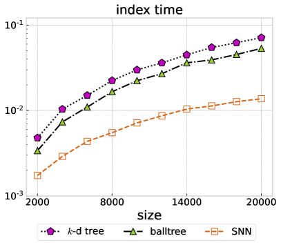
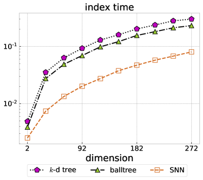
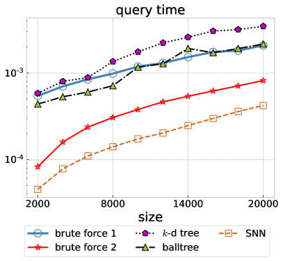
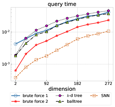
Figure 2: Comparing SNN to brute force search and tree-based methods. Total index time (top) and average query time (bottom) for the synthetic uniformly distributed dataset, all in seconds, as the data size $n$ is varied (left) or the dimension $d$ is varied (right). Brute force query methods do not require an index construction, hence are omitted on the left. Our SNN method is the best performer in all cases, in some cases 10 times faster than the best tree-based method (balltree).

6.2 Comparison with GriSPy

GriSPy (Chalela et al.,, 2021), perhaps the most recent work on fixed-radius NN search, is an exact search algorithm which claims to be superior over the tree-based algorithms in SciPy. GriSPy indexes the data points into regular grids and creates a hash table in which the keys are the cell coordinates, and the values are lists containing the indices of the points within the corresponding cell. As there is an open-source implementation available, we can easily compare GriSPy against SNN. However, GriSPy has a rather high memory demand which forced us to perform a separate experiments with reduced data sizes and dimensions as compared to the ones in the previous Section 6.1.

Again we consider $n$ uniformly distributed data points in $[0,1]^{d}$, but now with (i) varying data size from $n=1,000$ to $100,000$ and averaging the runtime of five different radius queries with $R=0.05,0.1,\ldots,0.25$, and (ii) varying dimension over $d=2,3,4$. The precise parameters and the corresponding ratio of returned data points are listed in Table 2. All queries are repeated 1,000 times and timings are averaged. Both experiments (i) and (ii) use the same query size as the index size.

The index and query timings are illustrated in Figure 3. We find that SNN indexing is about an order of magnitude faster than GriSPy over all tested parameters. For the experiment (i) where the data size is varied, we find that SNN is up to two orders of magnitude faster than GriSPy. For experiment (ii), we see that the SNN query time is more stable than GriSPy with respect to increasing data dimension.

Table 2: The table shows the ratio of returned data points from the synthetic uniformly distributed dataset, relative to the overall number of points $n$, as the data volumn $n$, query radius $R$ and the dimension $d$ is varied.

Varying $n$		$n$	1,000	2,154	4,641	10,000	21,544	46,415	100,000
		$R=0.05$	0.05 %	0.05 %	0.048 %	0.049 %	0.05 %	0.05 %	0.049 %
		$R=0.10$	0.37 %	0.37 %	0.36 %	0.38 %	0.37 %	0.37 %	0.37 %
($d=3$)		$R=0.15$	1.2 %	1.2 %	1.2 %	1.2 %	1.2 %	1.2 %	1.2 %
	$R=0.20$	2.6 %	2.6 %	2.6 %	2.7 %	2.7 %	2.6 %	2.6 %
	$R=0.25$	4.8 %	4.8 %	4.8 %	4.9 %	4.9 %	4.9 %	4.7 %
Varying $d$		$d$	2	3	4
		$R=0.05$	0.75 %	0.05 %	0.0029 %
		$R=0.10$	2.9 %	0.38 %	0.042 %
($n=$ 10,000)		$R=0.15$	6.1 %	1.2 %	0.2 %
	$R=0.20$	10 %	2.7 %	0.59 %
	$R=0.25$	15 %	4.9 %	1.3 %

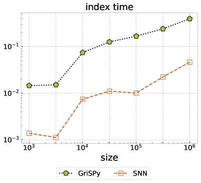
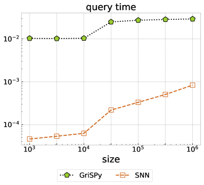
Figure 3: Comparing GriSPy and SNN. Total index time (top) and average query time (bottom) for on uniformly distributed data, all in seconds, as the data size $n$ is varied (left) or the dimension $d$ is varied (right). Our SNN method significantly outperforms GriSPy both in terms of indexing and query runtime.

6.3 Near neighbor query on real-world data

We now compare various fixed-radius NN search methods on datasets from the benchmark collection by Aumüller et al., (2020): Fashion-MNIST (abbreviated as F-MNIST), SIFT, GIST, GloVe100, and DEEP1B. Each dataset has an index set of $n$ points and a separate out-of-sample query set with $n^{\prime}<n$ points. See Table 3 for a summary of the data.

Table 4 lists the timings for the index construction of the tree-based methods and SNN. For all datasets, SNN is least 5.9 times faster than balltree (the fasted tree-based method). Significant speedups are gained in particular for large datasets: for the largest dataset DEEP1B, SNN creates its index more than 32 times faster than balltree.

Table 3: Summary of the real-world datasets

Dataset	Dimension $d$	Distance	Index size $n$	Query size $n^{\prime}$	Related reference
F-MNIST	784	Euclidean	25,000	10,000	(Xiao et al.,, 2017)
SIFT10K	128	Euclidean	25,000	100	(Lowe,, 2004)
SIFT1M	128	Euclidean	100,000	10,000	(Lowe,, 2004)
GIST	960	Euclidean	1,000,000	1,000	(Oliva and Torralba,, 2004)
GloVe100	100	Angular	1,183,514	10,000	(Pennington et al.,, 2014)
DEEP1B	96	Angular	9,990,000	10,000	(Yandex and Lempitsky,, 2016)

The query times averaged over all $n^{\prime}$ points from the query set are listed in Table 5. We have included tests over different radii $R$ in order to obtain a good order-of-magnitude variation in the number of returned nearest neighbors relative to the index size $n$, assessing the algorithms over a range of possible scenarios from small to large query returns. See the return ratios $\overline{\upsilon}$ listed in Table 5. Again, in all cases, SNN consistently performs the fastest queries over all datasets and radii. SNN is between about 6 and 14 times faster than balltree (the fastest tree-based method). For the datasets GloVe100 and DEEP1B, SNN displays the lowest speedup of about 1.6 compared to our brute force 2 implementation, indicating that for these datasets the sorting-based exclusion criterion does not significantly prune the search space. (These are datasets for which the angular distance is used, i.e., all data points are projected onto the unit sphere.) For the other datasets, SNN achieves significant speedups between 2.6 and 5.6 compared to brute force 2, owing to effective search space pruning.

Table 4: Index time in milliseconds for fixed-radius NN search on the real-world datasets (rounded to four significant digits). Lower is better and the best values are highlighted in bold.

Dataset	$k$-d tree	balltree	SNN
F-MNIST	9035	7882	1335
SIFT10K	720.5	662.1	79.1
SIFT1M	3292	2921	179
GIST	319400	297900	29140
GloVe100	41210	39800	1549
DEEP1B	446000	464100	14730

Table 5: Query time per data point in milliseconds for real-world data, averaged over $n^{\prime}$ out-of-sample queries. The search radius is $R$ and $\overline{\upsilon}$ is the average ratio of returned data points relative to the overall number of data points $n$. Lower is better and the best values are highlighted in bold.

Dataset	$R$	$\overline{\upsilon}$	brute force 1	brute force 2	$k$-d tree	balltree	SNN
F-MNIST	800	0.01524 %	302.8	43.99	146.3	110.3	7.765
	900	0.04008 %	244.4	43.96	152.2	110.7	8.602
	1000	0.09283 %	218.5	44.1	157.2	111.2	9.413
	1100	0.1960 %	217.3	44.28	160.5	111.5	10.21
	1200	0.3818 %	216.2	44.32	163.3	110.8	11.18
SIFT10K	210	0.02296%	19.04	4.187	15.88	12.55	1.112
	230	0.04892%	21.56	4.153	18.58	13.75	1.170
	250	0.1147%	21.24	4.546	18.35	13.15	1.458
	270	0.2718%	22.97	4.279	19.91	14.73	1.128
	290	0.5958%	22.06	4.276	19.86	15.33	1.093
SIFT1M	210	0.02661%	75.82	16.10	45.71	35.11	4.525
	230	0.05671%	78.24	16.15	46.86	38.37	4.557
	250	0.1231%	86.03	16.29	50.30	40.75	4.598
	270	0.2663%	80.13	16.17	54.13	42.76	4.660
	290	0.5608%	69.77	16.17	58.80	44.55	4.727
GIST	0.80	0.1430 %	3955	862.2	3144	2160	281.5
	0.85	0.1977%	3966	861.4	3182	2164	293.9
	0.90	0.2723%	3941	861.6	3206	2171	305.8
	0.95	0.3762%	3817	861.7	3223	2178	316.8
	1.00	0.5234%	3759	861.4	3237	2183	326.8
GloVe100	0.30 $\pi$	0.04506%	516.9	127.3	671.5	567.5	78.38
	0.31 $\pi$	0.07888%	514.1	126.9	673.2	561.8	79.47
	0.32 $\pi$	0.1438%	514.7	126.8	670.6	564.9	76.83
	0.33 $\pi$	0.2755%	520.1	126.5	674.9	561.0	77.27
	0.34 $\pi$	0.5507%	522.0	127.8	674.6	562.2	77.00
DEEP1B	0.22 $\pi$	0.04495%	4281	1079	5711	4731	803.0
	0.24 $\pi$	0.09332%	4229	1065	5677	4704	704.8
	0.26 $\pi$	0.1891%	4202	1082	5732	4683	719.9
	0.28 $\pi$	0.3761%	4230	1080	5765	4755	734.3
	0.30 $\pi$	0.7341%	4274	1084	5644	4810	723.1

6.4 An application to clustering

We now wish to demonstrate the performance gains that can be obtained with SNN using the DBSCAN clustering method (Campello et al.,, 2015; Jang and Jiang,, 2019) as an example. To this end we replace the nearest neighbor search method in scikit-learn’s DBSCAN implementation with SNN. To enure all variants perform the exact same NN queries, we rewrite all batch NN queries into loops of single queries and force all computations to run in a single threat. Except these modifications, DBSCAN remains unchanged and in all case returns exactly the same result when called on the same data and with the same hyperparameters (eps and min_sample).

We select datasets from the UCI Machine Learning Repository (Dua and Graff,, 2017); see Table 6. All datasets are pre-processed by z-score standardization (i.e., we shift each feature to zero mean and scale it to unit variance). We cluster the data for various choices of DBSCAN’s eps parameter and list the measured total runtime in Table 7. The parameter eps has the same interpretation as SNN’s radius parameter $R$. In all cases, we have fixed DBSCAN’s second hyperparameter min_sample at $5$. The normalized mutual information (NMI) (Cover and Thomas,, 2006) of the obtained clusterings is also listed in Table 7.

The runtimes in Table 7 show that DBSCAN with SNN is a very promising combination, consistently outperforming the other combinations. When compared to using non-batched and non-parallelized DBSCAN with balltree, DBSCAN with SNN performs between 3.5 and 16 times faster while returning precisely the same clustering results.

Table 6: Clustering datasets in the UCI Machine Learning Repository

Dataset	Size $n$	Dimension $d$	# Labels	Related references
Banknote	1372	4	2	Dua and Graff, (2017)
Dermatology	366	34	6	Dua and Graff, (2017); Güvenir et al., (1998)
Ecoli	336	7	8	Dua and Graff, (2017); Nakai and Kanehisa, (1991, 1992)
Phoneme	4509	256	5	Hastie et al., (2009)
Wine	178	13	3	Forina et al., (1998)

Table 7: Total DBSCAN runtime in milliseconds when different NN search algorithms are used. The DBSCAN radius parameter is eps and the achieved normalized mutual information is NMI. Best runtimes are highlighted in bold.

Dataset	eps	NMI	brute force	$k$-d tree	balltree	SNN
Banknote	0.1	0.05326	1,914	463.9	431.9	30.20
	0.2	0.2198	1,739	454.5	434.3	48.67
	0.3	0.3372	1,968	452.0	438.8	50.61
	0.4	0.5510	1,759	457.5	442.4	51.21
	0.5	0.08732	1,752	477.2	449.8	53.01
Dermatology	5.0	0.5568	706.8	138.8	124.3	86.81
	5.1	0.5714	654.0	142.2	127.8	64.62
	5.2	0.5733	651.8	139.2	123.2	63.74
	5.3	0.5796	650.7	138.2	121.5	60.75
	5.4	0.4495	638.6	138.4	121.2	58.17
Ecoli	0.5	0.1251	506.9	116.0	104.9	7.674
	0.6	0.2820	491.9	116.0	105.2	8.105
	0.7	0.3609	496.0	116.5	107.2	9.263
	0.8	0.4374	500.9	116.7	105.1	10.97
	0.9	0.1563	499.8	116.3	105.0	11.39
Phoneme	8.5	0.5142	3,497	17,290	7,685	926.9
	8.6	0.5516	3,511	17,480	7,738	954.1
	8.7	0.5836	3,300	17,490	7,727	937.9
	8.8	0.6028	3,257	17,600	7,768	975.2
	8.9	0.5011	3,499	17,570	7,734	1,065
Wine	2.2	0.4191	73.37	64.02	56.70	5.753
	2.3	0.4764	64.65	63.84	56.29	5.703
	2.4	0.5271	66.91	63.26	55.74	5.612
	2.5	0.08443	67.29	63.11	56.34	6.106
	2.6	0.07886	67.12	63.45	56.25	6.094

7 Conclusions

We presented a fixed-radius nearest neighbor (NN) search method called SNN. Compared to other exact NN search methods based on $k$-d tree or balltree data structures, SNN is trivial to implement and exhibits faster index and query time. We also demonstrated that SNN outperforms different implementations of brute force search. Just like brute force search, SNN requires no parameter tuning and is straightforward to use. We believe that SNN could become a valuable tool in applications such as the MultiDark Simulation (Klypin et al.,, 2016) or the Millennium Simulation (Boylan-Kolchin et al.,, 2009). We also demonstrated that SNN can lead to significant performance gains when used for nearest neighbor search within the DBSCAN clustering method.

While we have demonstrated SNN speedups in single-threaded computations on a CPU, we believe that the method’s reliance on high-level BLAS operations makes it suitable for parallel GPU computations. A careful CUDA implementation of SNN and extensive testing will be subject of future work.

References

- Alshammari et al., (2021) Alshammari, M., Stavrakakis, J., and Takatsuka, M. (2021). Refining a -nearest neighbor graph for a computationally efficient spectral clustering. Pattern Recognition, 114:107869.
- Aumüller et al., (2020) Aumüller, M., Bernhardsson, E., and Faithfull, A. (2020). ANN-Benchmarks: A benchmarking tool for approximate nearest neighbor algorithms. Information Systems, 87:101374.
- Bachrach et al., (2014) Bachrach, Y., Finkelstein, Y., Gilad-Bachrach, R., Katzir, L., Koenigstein, N., Nice, N., and Paquet, U. (2014). Speeding up the Xbox recommender system using a Euclidean transformation for inner-product spaces. In Proceedings of the 8th ACM Conference on Recommender Systems, RecSys ’14, pages 257–264. ACM.
- Bawa et al., (2005) Bawa, M., Condie, T., and Ganesan, P. (2005). Lsh forest: Self-tuning indexes for similarity search. In Proceedings of the 14th International Conference on World Wide Web, WWW ’05, pages 651–660. ACM.
- (5) Bentley, J. L. (1975a). Multidimensional binary search trees used for associative searching. Communications of the ACM, 18(9):509–517.
- (6) Bentley, J. L. (1975b). A survey of techniques for fixed radius near neighbor searching. Technical report, Stanford University.
- Beygelzimer et al., (2006) Beygelzimer, A., Kakade, S., and Langford, J. (2006). Cover trees for nearest neighbor. In Proceedings of the 23rd International Conference on Machine Learning, ICML ’06, pages 97–104. ACM.
- Blackford et al., (2002) Blackford, L., Demmel, J., Dongarra, J., Duff, I., Hammarling, S., Henry, G., Heroux, M., Kaufman, L., Lumsdaine, A., Petitet, A., Pozo, R., Remington, K., and Whaley, R. (2002). An updated set of basic linear algebra subprograms (BLAS). ACM Transactions on Mathematical Software, 28(2):135–151.
- Boylan-Kolchin et al., (2009) Boylan-Kolchin, M., Springel, V., White, S. D. M., Jenkins, A., and Lemson, G. (2009). Resolving cosmic structure formation with the Millennium-II Simulation. Monthly Notices of the Royal Astronomical Society, 398(3):1150–1164.
- Campello et al., (2013) Campello, R. J. G. B., Moulavi, D., and Sander, J. (2013). Density-based clustering based on hierarchical density estimates. In Advances in Knowledge Discovery and Data Mining, pages 160–172. Springer.
- Campello et al., (2015) Campello, R. J. G. B., Moulavi, D., Zimek, A., and Sander, J. (2015). Hierarchical density estimates for data clustering, visualization, and outlier detection. ACM Transactions on Knowledge Discovery from Data, 10:1–51.
- Cayton and Dasgupta, (2007) Cayton, L. and Dasgupta, S. (2007). A learning framework for nearest neighbor search. In Advances in Neural Information Processing Systems, volume 20. Curran Associates, Inc.
- Chakrabarti et al., (2002) Chakrabarti, K., Keogh, E., Mehrotra, S., and Pazzani, M. (2002). Locally adaptive dimensionality reduction for indexing large time series databases. ACM Transactions on Database Systems, 27(2):188–228.
- Chalela et al., (2021) Chalela, M., Sillero, E., Pereyra, L., Garcia, M., Cabral, J., Lares, M., and Merchán, M. (2021). Grispy: A Python package for fixed-radius nearest neighbors search. Astronomy and Computing, 34:100443.
- Cover and Thomas, (2006) Cover, T. M. and Thomas, J. A. (2006). Elements of Information Theory (Wiley Series in Telecommunications and Signal Processing). Wiley.
- Dasgupta and Sinha, (2013) Dasgupta, S. and Sinha, K. (2013). Randomized partition trees for exact nearest neighbor search. In Proceedings of the 26th Annual Conference on Learning Theory, volume 30 of Proceedings of Machine Learning Research, pages 317–337. PMLR.
- Datar et al., (2004) Datar, M., Immorlica, N., Indyk, P., and Mirrokni, V. S. (2004). Locality-sensitive hashing scheme based on p-stable distributions. In Proceedings of the 20th Annual Symposium on Computational Geometry, SCG ’04, pages 253–262. ACM.
- Dong et al., (2020) Dong, Y., Indyk, P., Razenshteyn, I., and Wagner, T. (2020). Learning space partitions for nearest neighbor search. In International Conference on Learning Representations.
- Dua and Graff, (2017) Dua, D. and Graff, C. (2017). UCI Machine Learning Repository.
- Ester et al., (1996) Ester, M., Kriegel, H.-P., Sander, J., and Xu, X. (1996). A density-based algorithm for discovering clusters in large spatial databases with noise. In Proceedings of the 2nd International Conference on Knowledge Discovery and Data Mining, KDD’96, pages 226–231. AAAI Press.
- Forina et al., (1998) Forina, M., Leardi, R., C, A., and Lanteri, S. (1998). PARVUS: an extendable package of programs for data exploration, classification and correlation. Journal of Chemometrics, 4:191–193.
- Francis-Landau and Durme, (2019) Francis-Landau, M. and Durme, B. V. (2019). Exact and/or fast nearest neighbors. arXiv, (1910.02478).
- Friedman et al., (1977) Friedman, J. H., Bentley, J. L., and Finkel, R. A. (1977). An algorithm for finding best matches in logarithmic expected time. ACM Transactions on Mathematical Software, 3(3):209–226.
- Gallego et al., (2018) Gallego, A.-J., Calvo-Zaragoza, J., Valero-Mas, J. J., and Rico-Juan, J. R. (2018). Clustering-based -nearest neighbor classification for large-scale data with neural codes representation. Pattern Recognition, 74:531–543.
- Gallego et al., (2022) Gallego, A. J., Rico-Juan, J. R., and Valero-Mas, J. J. (2022). Efficient -nearest neighbor search based on clustering and adaptive values. Pattern Recognition, 122:108356.
- Galvelis and Sugita, (2017) Galvelis, R. and Sugita, Y. (2017). Neural network and nearest neighbor algorithms for enhancing sampling of molecular dynamics. Journal of Chemical Theory and Computation, 13(6):2489–2500.
- Garcia et al., (2008) Garcia, V., Debreuve, E., and Barlaud, M. (2008). Fast k nearest neighbor search using GPU. In IEEE Computer Society Conference on Computer Vision and Pattern Recognition Workshops, pages 1–6.
- Geng et al., (2008) Geng, X., Liu, T.-Y., Qin, T., Arnold, A., Li, H., and Shum, H.-Y. (2008). Query dependent ranking using k-nearest neighbor. In Proceedings of the 31st Annual International ACM SIGIR Conference on Research and Development in Information Retrieval, SIGIR ’08, pages 115–122. ACM.
- Groß et al., (2019) Groß, J., Köster, M., and Krüger, A. (2019). Fast and efficient nearest neighbor search for particle simulations. In Computer Graphics & Visual Computing.
- Guo et al., (2020) Guo, R., Sun, P., Lindgren, E., Geng, Q., Simcha, D., Chern, F., and Kumar, S. (2020). Accelerating large-scale inference with anisotropic vector quantization. In Proceedings of the 37th International Conference on Machine Learning, volume 119 of Proceedings of Machine Learning Research, pages 3887–3896. PMLR.
- Güvenir et al., (1998) Güvenir, H. A., Demiröz, G., and Ilter, N. (1998). Learning differential diagnosis of erythemato-squamous diseases using voting feature intervals. Artificial Intelligence in Medicine, 13:147–65.
- Hastie et al., (2009) Hastie, T., Tibshirani, R., and Friedman, J. (2009). The Elements of Statistical Learning: Data Mining, Inference, and Prediction. Springer, 2 edition.
- Higham, (2002) Higham, N. J. (2002). Accuracy and Stability of Numerical Algorithms. SIAM, 2 edition.
- Indyk and Motwani, (1998) Indyk, P. and Motwani, R. (1998). Approximate nearest neighbors: towards removing the curse of dimensionality. In Proceedings of the 30th Annual ACM Symposium on Theory of Computing, STOC ’98, pages 604–613. ACM.
- Jang and Jiang, (2019) Jang, J. and Jiang, H. (2019). DBSCAN++: Towards fast and scalable density clustering. In Proceedings of the 36th International Conference on Machine Learning, volume 97 of Proceedings of Machine Learning Research, pages 3019–3029. PMLR.
- Kaminska et al., (2021) Kaminska, O., Cornelis, C., and Hoste, V. (2021). Nearest neighbour approaches for emotion detection in tweets. In Proceedings of the 11th Workshop on Computational Approaches to Subjectivity, Sentiment and Social Media Analysis, pages 203–212. Association for Computational Linguistics.
- Keogh and Ratanamahatana, (2005) Keogh, E. and Ratanamahatana, C. A. (2005). Exact indexing of dynamic time warping. Knowledge and Information Systems, 7(3):358–386.
- Klypin et al., (2016) Klypin, A., Yepes, G., Gottlöber, S., Prada, F., and Heß, S. (2016). MultiDark simulations: the story of dark matter halo concentrations and density profiles. Monthly Notices of the Royal Astronomical Society, 457(4):4340–4359.
- Li et al., (2020) Li, H., Liu, X., Li, T., and Gan, R. (2020). A novel density-based clustering algorithm using nearest neighbor graph. Pattern Recognition, 102:107206.
- Lowe, (2004) Lowe, D. G. (2004). Distinctive image features from scale-invariant keypoints. International Journal of Computer Vision, 60(2):91–110.
- Malkov and Yashunin, (2020) Malkov, Y. A. and Yashunin, D. A. (2020). Efficient and robust approximate nearest neighbor search using hierarchical navigable small world graphs. IEEE Transactions on Pattern Analysis and Machine Intelligence, 42(4):824–836.
- Muja, (2013) Muja, M. (2013). Scalable nearest neighbour methods for high dimensional data. PhD thesis, University of British Columbia.
- Muja and Lowe, (2009) Muja, M. and Lowe, D. G. (2009). Flann, fast library for approximate nearest neighbors. In International Conference on Computer Vision Theory and Applications, volume 3 of VISAPP’09, pages 1–21.
- Nakai and Kanehisa, (1991) Nakai, K. and Kanehisa, M. (1991). Expert system for predicting protein localization sites in gram-negative bacteria. Proteins, 11:95–110.
- Nakai and Kanehisa, (1992) Nakai, K. and Kanehisa, M. (1992). A knowledge base for predicting protein localization sites in eukaryotic cells. Genomics, 14:897–911.
- Nister and Stewenius, (2006) Nister, D. and Stewenius, H. (2006). Scalable recognition with a vocabulary tree. In IEEE Computer Society Conference on Computer Vision and Pattern Recognition (CVPR’06), volume 2, pages 2161–2168.
- Oliva and Torralba, (2004) Oliva, A. and Torralba, A. (2004). Modeling the shape of the scene: a holistic representation of the spatial envelope. International Journal of Computer Vision, 42:145–175.
- Omohundro, (1989) Omohundro, S. M. (1989). Five balltree construction algorithms. Technical report, International Computer Science Institute.
- Pedregosa et al., (2011) Pedregosa, F., Varoquaux, G., Gramfort, A., Michel, V., Thirion, B., Grisel, O., Blondel, M., Prettenhofer, P., Weiss, R., Dubourg, V., Vanderplas, J., Passos, A., Cournapeau, D., Brucher, M., Perrot, M., and Duchesnay, E. (2011). Scikit-learn: machine learning in Python. Journal of Machine Learning Research, 12:2825–2830.
- Pennington et al., (2014) Pennington, J., Socher, R., and Manning, C. D. (2014). GloVe: Global vectors for word representation. In Empirical Methods in Natural Language Processing, pages 1532–1543.
- Philbin et al., (2007) Philbin, J., Chum, O., Isard, M., Sivic, J., and Zisserman, A. (2007). Object retrieval with large vocabularies and fast spatial matching. In IEEE Conference on Computer Vision and Pattern Recognition, pages 1–8.
- Ram and Sinha, (2019) Ram, P. and Sinha, K. (2019). Revisiting kd-tree for nearest neighbor search. In Proceedings of the 25th ACM SIGKDD International Conference on Knowledge Discovery & Data Mining, KDD ’19, pages 1378–1388. ACM.
- Shakhnarovich et al., (2003) Shakhnarovich, Viola, and Darrell (2003). Fast pose estimation with parameter-sensitive hashing. In Proceedings 9th IEEE International Conference on Computer Vision, volume 2, pages 750–757.
- Silpa-Anan and Hartley, (2008) Silpa-Anan, C. and Hartley, R. (2008). Optimised KD-trees for fast image descriptor matching. In IEEE Conference on Computer Vision and Pattern Recognition, pages 1–8.
- The MathWorks Inc., (2022) The MathWorks Inc. (2022). Matlab version: 9.13.0 (r2022b).
- Virtanen et al., (2020) Virtanen, P., Gommers, R., Oliphant, T. E., Haberland, M., Reddy, T., Cournapeau, D., Burovski, E., Peterson, P., Weckesser, W., Bright, J., van der Walt, S. J., Brett, M., Wilson, J., Millman, K. J., Mayorov, N., Nelson, A. R. J., Jones, E., Kern, R., Larson, E., Carey, C. J., Polat, İ., Feng, Y., Moore, E. W., VanderPlas, J., Laxalde, D., Perktold, J., Cimrman, R., Henriksen, I., Quintero, E. A., Harris, C. R., Archibald, A. M., Ribeiro, A. H., Pedregosa, F., van Mulbregt, P., and SciPy 1.0 Contributors (2020). SciPy 1.0: Fundamental Algorithms for Scientific Computing in Python. Nature Methods, 17:261–272.
- Wang et al., (2015) Wang, H., Liu, A., Wang, J., Ziebart, B. D., Yu, C. T., and Shen, W. (2015). Context retrieval for web tables. In Proceedings of the 2015 International Conference on The Theory of Information Retrieval, ICTIR ’15, pages 251–260. ACM.
- Xiao et al., (2017) Xiao, H., Rasul, K., and Vollgraf, R. (2017). Fashion-MNIST: a novel image dataset for benchmarking machine learning algorithms. arXiv, (1708.07747).
- Yagoubi et al., (2020) Yagoubi, D.-E., Akbarinia, R., Masseglia, F., and Palpanas, T. (2020). Massively distributed time series indexing and querying. IEEE Transactions on Knowledge and Data Engineering, 32(1):108–120.
- Yandex and Lempitsky, (2016) Yandex, A. B. and Lempitsky, V. (2016). Efficient indexing of billion-scale datasets of deep descriptors. In IEEE Conference on Computer Vision and Pattern Recognition, pages 2055–2063. IEEE.
- Yianilos, (1993) Yianilos, P. N. (1993). Data structures and algorithms for nearest neighbor search in general metric spaces. In Proceedings of the 4th Annual ACM-SIAM Symposium on Discrete Algorithms, SODA ’93, pages 311–321. SIAM.