Data-driven Stochastic Output-Feedback Predictive Control: Recursive Feasibility through Interpolated Initial Conditions

Abstract

The paper investigates data-driven output-feedback predictive control of linear systems subject to stochastic disturbances. The scheme relies on the recursive solution of a suitable data-driven reformulation of a stochastic Optimal Control Problem (OCP), which allows for forward prediction and optimization of statistical distributions of inputs and outputs. Our approach avoids the use of parametric system models. Instead it is based on previously recorded data using a recently proposed stochastic variant of Willems’ fundamental lemma. The stochastic variant of the lemma is applicable to a large class of linear dynamics subject to stochastic disturbances of Gaussian and non-Gaussian nature. To ensure recursive feasibility, the initial condition of the OCP—which consists of information about past inputs and outputs—is considered as an extra decision variable of the OCP. We provide sufficient conditions for recursive feasibility and closed-loop practical stability of the proposed scheme as well as performance bounds. Finally, a numerical example illustrates the efficacy and closed-loop properties of the proposed scheme.

1 Introduction

Data-driven control based on the so-called fundamental lemma by [Willems et al. (2005)] has attracted a lot of research interest, see [Markovsky and Dörfler (2021), De Persis and Tesi (2020)] for recent reviews. The pivotal insight of the fundamental lemma is that any controllable LTI system can be characterized by its recorded input-output trajectories provided a persistency of excitation condition to be satisfied. In the context of predictive control this implies that the prediction of future input and output trajectories can be done based on measurements of past trajectories thus alleviating the need for system identification and state estimator design (Yang and Li, 2015; Coulson et al., 2019; Lian and Jones, 2021; Allibhoy and Cortes, 2020). Hence data-driven predictive control schemes are consider for different applications, e.g. (Carlet et al., 2023; Bilgic et al., 2022; Wang et al., 2022a). Rigorous stability guarantees are provided by Berberich et al. (2020, 2021); Bongard et al. (2022) for data-driven predictive control schemes with respect to deterministic LTI systems subjected to noisy measurements.

However, besides measurement noise, so far little has been done on data-driven predictive control for LTI systems subject to stochastic disturbances. One key challenge is the prediction of the future evolution of statistical distributions of the inputs (respectively input policies) and outputs in a data-driven fashion. One approach is to predict the expected value of the future trajectory by the fundamental lemma while handling the stochastic uncertainties offline by probabilistic constraint tightening (Kerz et al., 2021) or directly omitting the stochastic uncertainties in the prediction (Wang et al., 2022b). Alternatively, leveraging the framework of Polynomial Chaos Expansions (PCE) (Sullivan, 2015) a stochastic variant of Willems’ fundamental lemma has been proposed (Pan et al., 2022b). It allows to predict future statistical distributions of inputs and outputs via previously recorded data and knowledge about the distribution of the disturbance.

Extending the conceptual ideas of Pan et al. (2022b) towards stochastic data-driven predictive control with guarantees, Pan et al. (2022c) present first results in a state-feedback setting, while the output-feedback case is discussed by Pan et al. (2022a). Therein, sufficient conditions of recursive feasibility and stability are provided by a data-driven design of terminal ingredients and a selection strategy of the initial condition which is similar to the model-based approach of Farina et al. (2013, 2015). The selection of initial conditions considers a binary choices: the current measured value or its predicted value based on the last optimal solution.

In this paper, we extend the data-driven stochastic output-feedback predictive scheme proposed by Pan et al. (2022a) with an improved initialization strategy. Instead of the binary selection strategy described above, the proposed scheme interpolates between the measured value and the latest prediction in a continuous fashion. In model-based stochastic predictive control this has been considered by Köhler and Zeilinger (2022); Schlüter and Allgöwer (2022). The main contribution of the present paper are sufficient conditions for stability and recursive feasibility of the proposed data-driven stochastic output-feedback scheme.

2 Problem statement and preliminaries

We investigate a data-driven stochastic output feedback approach to control of LTI systems with unknown system matrices. Hence, we first detail the considered setting, then we recall the representation of $\mathcal{L}^{2}$ random variables via polynomial chaos, before we arrive at the stochastic fundamental lemma.

2.1 Considered system class

We consider stochastic LTI systems in AutoRegressive with eXtra input (ARX) form

$$Y_{k}=\Phi Z_{k}+DU_{k}+W_{k},\quad Z_{0}=Z_{{\text{ini}}},$$ (1)

with input $U_{k}\in\mathcal{L}^{2}(\Omega,\mathcal{F},\mu;\mathbb{R}^{{n_{u}}})$, output $Y_{k}\in$ $\mathcal{L}^{2}(\Omega,\mathcal{F},\mu;\mathbb{R}^{{n_{y}}})$, disturbance $W_{k}\in$ $\mathcal{L}^{2}(\Omega,\mathcal{F},\mu;\mathbb{R}^{{n_{w}}})$ $({n_{w}}={n_{y}})$, and extended state

$$Z\doteq\begin{bmatrix}\mathbf{U}_{[k-{T_{\text{ini}}},k-1]}\\ \mathbf{Y}_{[k-{T_{\text{ini}}},k-1]}\end{bmatrix}=\left[U_{k-{T_{\text{ini}}}}^{\top},U_{k-{T_{\text{ini}}}+1}^{\top},\cdots,U_{k-1}^{\top},Y_{k-{T_{\text{ini}}}}^{\top},\cdots,Y_{k-1}^{\top}\right]^{\top}\in\mathcal{L}^{2}(\Omega,\mathcal{F},\mu;\mathbb{R}^{{n_{z}}}),$$

with ${n_{z}}={T_{\text{ini}}}({n_{u}}+{n_{y}})$ which contains last ${T_{\text{ini}}}$ inputs and outputs.

Here, $\Omega$ denotes the sample space, $\mathcal{F}$ is a $\sigma$ algebra, and $\mu$ is the considered probability measure. With the specification of the underlying probability space $(\Omega,\mathcal{F},\mu)$ to be $\mathcal{L}^{2}$, we restrict the consideration to random variables with finite expectation and finite (co)-variance. Throughout this paper, the system matrices $\Phi\in\mathbb{R}^{{n_{y}}\times{n_{z}}}$ and $D\in\mathbb{R}^{{n_{y}}\times{n_{u}}}$ are considered to be unknown, while the statistical distributions of initial condition $Z_{{\text{ini}}}$ and disturbances $\{W_{k}\}_{k\in\mathbb{N}}$ are supposed to be known. Furthermore, we consider that all $\{W_{k}\}_{k\in\mathbb{N}}$ are identical independently distributed ($i.i.d.$) with zero mean and finite co-variance, i.e., we assume for all $k\in\mathbb{N}$, $\mathbb{E}[W_{k}]=0$ and $\Sigma[W_{k}]=\Sigma_{W}$. We remark that the initial condition and the disturbances are not restricted to be Gaussian.

For a specific uncertainty outcome $\omega\in\Omega$, we denote the realization of $W_{k}$ as $w_{k}\doteq W_{k}(\omega)$. Likewise, the input, output, and extended state realizations are written as $u_{k}\doteq U_{k}(\omega)$, $y_{k}\doteq Y_{k}(\omega)$, and $z_{k}\doteq Z_{k}(\omega)$, respectively. Moreover, given $z_{{\text{ini}}}$ and $w_{k}$, $k\in\mathbb{N}$, the stochastic system (1) induces the realization dynamics

$$y_{k}=\Phi z_{k}+Du_{k}+w_{k},\quad z_{0}=z_{{\text{ini}}}.$$ (2)

Throughout the paper, we assume the input, output, and disturbance realizations $u_{k}$, $y_{k}$, and $w_{k-1}$ to be measured at time instant $k$. For the case of unmeasured disturbances, we refer to the disturbance estimation schemes tailored to ARX models, see (Pan et al., 2022b; Wang et al., 2022b) .

Assumption 1 (Minimal state-space representation)

There exists a minimal state-space representation

$$X =AX+BU+EW,\quad X_{0}=X_{{\text{ini}}}$$ (3a)

$$Y =CX+DU+W,$$ (3b)

with $(A,B)$ controllable and $(A,C)$ observable such that for some initial condition $X_{{\text{ini}}}$ and $W_{k}$, $k\in\mathbb{N}$, the input-output trajectories of (1) and (3) coincide.

For insights into the problem of mapping a ARX model to its minimal state-space representations, see Sadamoto (2022); Wu (2022).

2.2 Representation of random variables via polynomial chaos expansions

It is well-known that for stochastic LTI systems subject to Gaussian disturbances, the evolution of statistical distributions of inputs (generated via affine policies) and outputs can be exactly represented by the first two moments, cf. Farina et al. (2013, 2015). However, this is not necessarily the case for non-Gaussian disturbances. Moreover, observe that already in a Gaussian setting moments constitute non-linear representations of random variables as any scalar Gaussian is given by the sum of its mean with its standard deviation ($=$ square root of variance) times a standard normal-distributed random variable. Alternatively, one could rely on scenario-based approach and sampling strategies (Kantas et al., 2009; Tempo et al., 2013; Schildbach et al., 2014). However, this induces substantial computational effort.

Alternatively, we employ Polynomial Chaos Expansions (PCE) to provide a tractable linear surrogate of (1) by representing $\mathcal{L}^{2}$ random variables in a suitable polynomial basis. PCE dates back to Wiener (1938), and we refer to Sullivan (2015) for a general introduction, see, e.g., (Paulson et al., 2014; Mesbah et al., 2014; Ou et al., 2021) for applications in control.

Consider an orthogonal polynomial basis $\{\phi^{j}\}_{j=0}^{\infty}$ which spans $\mathcal{L}^{2}(\Omega,\mathcal{F},\mu;\mathbb{R})$, i.e.,

$$\langle\phi^{i},\phi^{j}\rangle\doteq\int_{\Omega}\phi^{i}(\omega)\phi^{j}(\omega)\mathop{}\!\mathrm{d}\mu(\omega)=\delta^{ij}\|{\phi^{j}}\|_{\mathcal{L}^{2}}^{2},$$

where $\delta^{ij}$ is the Kronecker delta and $\|{V}\|_{\mathcal{L}^{2}}\doteq\sqrt{\langle V,V\rangle}$ represents the induced form of $V\in\mathcal{L}^{2}(\Omega,\mathcal{F},\mu;\mathbb{R})$. With respect to the basis $\{\phi^{j}\}_{j=0}^{\infty}$, a real-valued random scalar variable $V\in\mathcal{L}^{2}(\Omega,\mathcal{F},\mu;\mathbb{R})$ can be expressed as $V=\sum_{j=0}^{\infty}\mathsf{v}^{j}\phi^{j}$ with $\mathsf{v}^{j}=\langle V,\phi^{j}\rangle/\|{\phi^{j}}\|_{\mathcal{L}^{2}}^{2},$ where $\mathsf{v}^{j}\in\mathbb{R}$ is called the $j$-th PCE coefficient. For a vector-valued random variable $V\in\mathcal{L}^{2}(\Omega,\mathcal{F},\mu;\mathbb{R}^{n_{v}})$ applying PCE component-wise the $j$-th coefficient is given as $\mathsf{v}^{j}=$ $\begin{bmatrix}\mathsf{v}^{1,j}&\mathsf{v}^{2,j}&\cdots&\mathsf{v}^{n_{v},j}\end{bmatrix}^{\top}$ where $\mathsf{v}^{i,j}$ is the $j$-th PCE coefficient of the component $V^{i}$ of $V$.

In practice one often terminates the PCE series after a finite number of terms for more efficient computation. However, this may lead to truncation errors (Mühlpfordt et al., 2018). Fortunately, random variables that follow some widely-used distributions admit exact finite-dimensional PCEs with only two terms in suitable polynomial bases, see (Koekoek and Swarttouw, 1998; Xiu and Karniadakis, 2002). For example, the Legendre basis is preferably chosen for uniformly-distributed random variables and Hermite polynomials are used for Gaussians.

Definition 2.1 (Exact PCE representation (Mühlpfordt et al., 2018)).

The PCE of a random variable $V\in\mathcal{L}^{2}(\Omega,\mathcal{F},\mu;\mathbb{R}^{n_{v}})$ is said to be exact with dimension $L$ if $V-\sum_{j=0}^{L-1}\mathsf{v}^{j}\phi^{j}=0$.

Notice that with an exact PCE of finite dimension, the expected value, variance and covariance of $V\in\mathcal{L}^{2}(\Omega,\mathcal{F},\mu;\mathbb{R}^{n_{v}})$ can be efficiently calculated from its PCE coefficients

$$\mathbb{E}\big{[}V\big{]}=\mathsf{v}^{0},\quad\mathbb{V}\big{[}V\big{]}=\sum_{j=1}^{L-1}(\mathsf{v}^{j})^{2}\|{\phi^{j}}\|_{\mathcal{L}^{2}}^{2},\quad\Sigma\big{[}V\big{]}=\sum_{j=1}^{L-1}\mathsf{v}^{j}\mathsf{v}^{j\top}\|{\phi^{j}}\|_{\mathcal{L}^{2}}^{2},$$ (4)

where $(\mathsf{v}^{j})^{2}\doteq\mathsf{v}^{j}\circ\mathsf{v}^{j}$ denotes the Hadamard product (Lefebvre, 2021). Finally, observe that (finite or infinite) PCEs of $\mathcal{L}^{2}$ random variables constitute linear representations of random variables.

To the end of reformulation of (1) with finite dimensional PCEs, we assume that $Z_{{\text{ini}}}$ and $W_{k},k\in\mathbb{N}^{+}$ admit exact PCEs in the basis $\{\phi^{j}_{{\text{ini}}}\}_{j=0}^{L_{\text{ini}}-1}$, respectively, in the basis $\{\varphi_{k}^{j}\}_{j=0}^{L_{w}-1}$. Consider system (1) for a finite horizon $N\in\mathbb{N}$ and the finite-dimensional joint basis

$$\{\phi^{j}\}_{j=0}^{L-1}=\left\{1,\{\phi^{j}_{{\text{ini}}}\}_{j=1}^{L_{\text{ini}}-1},\bigcup_{i=0}^{N-1}\{\varphi_{i}^{j}\}_{j=1}^{L_{w}-1}\right\},\qquad L =L_{\text{ini}}+N(L_{w}-1)\in\mathbb{N}^{+}.$$ (5)

Then, for all $k\in\mathbb{I}_{[0,N-1]}$, $U_{k}$, $Y_{k}$, and thus $Z_{k}$ also admit exact PCEs in the chosen basis if $U_{k}$ is designed as an affine feedback of $Z_{k}$, cf. the formal proofs given in (Pan et al., 2022b, a). Note that the key aspect of $\{\phi^{j}\}_{j=0}^{L-1}$ is that it is the union of the bases for $Z_{{\text{ini}}}$ and $W_{k}$, $k\in\mathbb{I}_{[0,N-1]}$. Thus, PCE enables uncertainty propagation over any finite prediction horizon.

Replacing all random variables in (1) with their PCE representation in the basis $\{\phi^{j}\}_{j=0}^{L-1}$ and projecting onto the basis functions $\phi^{j}$, we obtain the dynamics of the PCE coefficients. For given $\mathsf{z}^{j}_{{\text{ini}}}$ and $\mathsf{w}^{j}_{k}$, $k\in\mathbb{N}$, the dynamics of the PCE coefficients read

$$\mathsf{y}^{j}_{k}=\Phi\mathsf{z}^{j}_{k}+D\mathsf{u}^{j}_{k}+\mathsf{w}^{j}_{k},\quad\mathsf{z}^{j}_{0}=\mathsf{z}^{j}_{{\text{ini}}},\quad j\in\mathbb{I}_{[0,L-1]}.$$ (6)

2.3 Data-driven system representation via the stochastic fundamental lemma

It is the linearity of the series expansion which ensures that the original stochastic system (1) and its PCE formulation (6) are structurally similar. Subsequently, we recall the stochastic variant of Willems’ fundamental lemma which exploits this structural similarity.

Definition 2.2 (Persistency of excitation (Willems et al., 2005)).

Let $T,t\in\mathbb{N}^{+}$. A sequence of real-valued inputs $\mathbf{u}_{[0,{T-1}]}$ is said to be persistently exciting of order $t$ if the Hankel matrix

$$\mathcal{H}_{t}(\mathbf{u}_{[0,{T-1}]})\doteq\begin{bmatrix}u&\cdots&u\\ \vdots&\ddots&\vdots\\ u&\cdots&u\\ \end{bmatrix}$$

is of full row rank.

Lemma 2.3 (Stochastic fundamental lemma (Pan et al., 2022b; Faulwasser et al., 2022)).

Let Assumption 1 hold, and consider the stochastic LTI system (1) and its $\mathcal{L}^{2}(\Omega,\mathcal{F}_{k},\mu;\mathbb{R}^{{n_{v}}})$, ${n_{v}}\in\{{n_{u}},{n_{w}},{n_{y}}\}$ trajectories of random variables and the corresponding realization trajectories from (2), which are $\mathbf{(U,W,Y)}_{[0,{T-1}]}$ and $\mathbf{(u,w,y)}_{[0,{T-1}]}$, respectively. Let $\mathbf{(u,w)}_{[0,{T-1}]}$ be persistently exciting of order ${n_{x}}+t$. Then $(\widetilde{\mathbf{U}},\widetilde{\mathbf{W}},\widetilde{\mathbf{Y}})_{[0,t-1]}$ is a trajectory of (1) if and only if there exists $G\in\mathcal{L}^{2}(\Omega,\mathcal{F},\mu;\mathbb{R}^{T-t+1})$ such that

$$\mathcal{H}_{t}(\mathbf{v}_{[0,{T-1}]})G=\widetilde{\mathbf{V}}_{[0,t-1]}$$ (7)

holds for all $(\mathbf{v},\widetilde{\mathbf{V}})\in\{(\mathbf{u},\widetilde{\mathbf{U}}),(\mathbf{w},\widetilde{\mathbf{W}}),(\mathbf{y},\widetilde{\mathbf{Y}})\}$.

Corollary 2.4 (PCE coefficients via realizations (Pan et al., 2022b; Faulwasser et al., 2022)).

Let the conditions of Lemma 2.3 hold. Then, for $j\in\mathbb{I}_{[0,L-1]}$, $\mathbf{(\tilde{\mathsf{u}},\tilde{\mathsf{w}},\tilde{\mathsf{y}})}_{[0,{t-1}]}^{j}$ is a PCE coefficient trajectory of (6) if and only if there exists a $\mathsf{g}^{j}\in\mathbb{R}^{T-t+1}$ such that

$$\mathcal{H}_{t}(\mathbf{v}_{[0,{T-1}]})\mathsf{g}^{j}=\mathbf{\tilde{\mathsf{v}}}_{[0,{t-1}]}^{j}$$ (8)

holds for all $(\mathbf{v},\tilde{\mathsf{v}})\in\{(\mathbf{u},\tilde{\mathsf{u}}),(\mathbf{w},\tilde{\mathsf{w}}),(\mathbf{y},\tilde{\mathsf{y}})\}$.

As the page limit prohibits the detailed discussion of the above we refer to Pan et al. (2022b); Faulwasser et al. (2022) for proofs and examples. However, the key insight underlying the above results is that the dynamics of random variables (1), its realization dynamics (2), and the dynamics of PCE coefficients (6) share the same system structure and matrices. Hence, their finite-length trajectories can be linked to the trajectories of realization dynamics (2) as shown in (7) and (8). Put differently, in (7) and (8) Hankel matrices in measured realization data are used to predict the future evolution of random variables.

3 Data-driven stochastic output-feedback predictive control

In this section, we extend the data-driven stochastic output-feedback predictive control Pan et al. (2022a) through interpolation of the initial condition. We provide sufficient conditions of recursive feasibility, performance, and stability of the extended scheme.

3.1 Data-driven stochastic OCP with interpolated initial conditions

Consider the stochastic LTI system (1), its realization dynamics (2), and its PCE coefficients dynamics (6) with respect to the basis $\{\phi^{j}\}_{j=0}^{L-1}$, cf. (5). Suppose that a realization trajectory $\mathbf{(u,w,y)}_{[0,{T-1}]}$ of (2) is available with $\mathbf{(u,w)}_{[0,{T-1}]}$ persistently exciting of order ${n_{x}}+N+{T_{\text{ini}}}$.

In the following, consider $\mathsf{v}^{[0,L-1]}\doteq[\mathsf{v}^{0\top},\mathsf{v}^{1\top},\dots,\mathsf{v}^{L-1\top}]^{\top}$ as the vectorization of PCE coefficients over PCE dimensions, and let $\mathsf{v}^{j}_{i|k}$ be the predicted value of $\mathsf{v}^{j}_{k+i}$ at time instant $k$, $\mathsf{v}\in\{\mathsf{u},\mathsf{y},\mathsf{z}\}$. At time instant $k\in\mathbb{N}$, given the PCE coefficients of the disturbances, i.e. $\mathsf{w}_{k+i}^{[0,L-1]}$, $i\in\mathbb{I}_{[0,N-1]}$, the realization of the current extended state $z_{k}$, and the predicted PCE coefficients from last step $\mathsf{z}^{[0,L-1],\star}_{1|k-1}$, we consider the following data-driven stochastic OCP

$$V_{N}\left(z_{k},\mathsf{z}^{[0,L-1],\star}_{1|k-1}\right)\doteq\min_{\mathsf{(u,y,z)}^{\cdot}_{\cdot|k},\mathsf{g}^{\cdot},\mu}\,\sum_{j=0}^{L-1}\|{\phi^{j}}\|_{\mathcal{L}^{2}}^{2}\left(\sum_{i=0}^{N-1}\Big{(}\|\mathsf{y}^{j}_{i|k}\|^{2}_{Q}+\|\mathsf{u}^{j}_{i|k}\|^{2}_{R}\Big{)}+\|\mathsf{z}^{j}_{N|k}\|_{P}^{2}\right)$$ (9a)

$$\text{subject to }\quad\left[\begin{array}[]{l}\mathcal{H}_{N+{T_{\text{ini}}}}(\mathbf{u}_{[0,{T-1}]})\\ \mathcal{H}_{N+{T_{\text{ini}}}}(\mathbf{y}_{[0,{T-1}]})\\ \mathcal{H}_{N}(\mathbf{w}_{[{T_{\text{ini}}},T-1]})\\ \end{array}\right]\mathsf{g}^{j}=\left[\begin{array}[]{l}\mathsf{u}^{j}_{[-{T_{\text{ini}}},N-1]|k}\\ \mathsf{y}^{j}_{[-{T_{\text{ini}}},N-1]|k}\\ \mathsf{w}^{j}_{[k,k+N-1]}\\ \end{array}\right],\quad\forall j\in\mathbb{I}_{[0,L-1]}$$ (9h)

$$\mathsf{z}^{[0,L-1]}_{0|k}\in\mathbb{Z}_{{\text{ini}}}\left(\mu,z_{k},\mathsf{z}^{[0,L-1],\star}_{1|k-1}\right)$$ (9i)

$$\mathsf{v}^{0}_{i|k}\pm\sigma(\varepsilon_{v})\sqrt{\sum_{j=1}^{L-1}{(\mathsf{v}^{j}_{i|k}})^{2}\langle\phi^{j}\rangle^{2}}\in\mathbb{V},\quad\mathsf{v}\in\{\mathsf{u},\mathsf{y}\},\quad\forall i\in\mathbb{I}_{[0,N-1]}$$ (9j)

$$\mathsf{u}_{i|k}^{j^{\prime}}=0,\quad\forall j^{\prime}\in\mathbb{I}_{[L_{\text{ini}}+i(L_{w}-1)+1,L-1]},\quad\forall i\in\mathbb{I}_{[0,N-1]},$$ (9k)

$$\mathsf{z}^{0}_{N|k}\in\mathbb{Z}_{\text{f}},\quad\sum_{j=1}^{L-1}\mathsf{z}^{j\top}_{N|k}\Gamma\mathsf{z}^{j}_{N|k}\|{\phi^{j}}\|_{\mathcal{L}^{2}}^{2}\leq\gamma,$$ (9l)

$$\mathsf{z}^{j}_{i|k}=\begin{bmatrix}\mathsf{u}^{j}_{[i-{T_{\text{ini}}},i-1]|k}\\ \mathsf{y}^{j}_{[i-{T_{\text{ini}}},i-1]|k}\end{bmatrix},\quad i\in\mathbb{I}_{[0,N]},\quad j\in\mathbb{I}_{[0,L-1]}.$$ (9m)

Observe that the decision variables $\mathsf{z}$ are redundant. They are introduced for the sake of compact notation and they can easily be avoided via (9m).

The objective function (9a) penalizes the predicted input and output PCE coefficients with $R=R^{\top}\succ 0$ and $Q=Q^{\top}\succ 0$. Moreover, $P=P^{\top}\succ 0$ characterizes the terminal cost with respect to the PCE coefficients $\mathsf{z}^{j}_{N|k}$. Formulated in terms of PCE coefficients, the objective function (9a) is equivalent to the expected value of its counterpart with random variables (Pan et al., 2022b). The linear equalities (9h)–(9i) encode the dynamics of the PCE coefficients (6) in a non-parametric fashion and based on measured data, cf. Lemma 2.3 and Corollary 2.4.

The initial condition of OCP (9) is considered in (9i). Given $\mathsf{z}^{[0,L-1],\star}_{1|k-1}$ as the predicted value of $\mathsf{z}^{j}_{k}$ with respect to the optimal solution at time instant $k-1$, we specify the constraint set in (9i) as

$$\mathbb{Z}_{{\text{ini}}}\doteq\left\{\mathsf{z}^{[0,L-1]}_{0|k}\middle|\begin{gathered}\mathsf{z}^{0}_{0|k}=\mu z_{k}+(1-\mu)\mathsf{z}^{0,\star}_{1|k-1},\quad 0\leq\mu\leq 1\\ \sum_{j=1}^{L_{{\text{ini}}}-1}\mathsf{z}^{j}_{0|k}\mathsf{z}^{j\top}_{0|k}\|{\phi^{j}}\|_{\mathcal{L}^{2}}^{2}=(1-\mu)^{2}\sum_{j=1}^{L-1}\mathsf{z}^{j,\star}_{1|k-1}\mathsf{z}^{j,\star\top}_{1|k-1}\|{\phi^{j}}\|_{\mathcal{L}^{2}}^{2}\\ \mathsf{z}^{j}_{0|k}=0,\quad j=\mathbb{I}_{[L_{{\text{ini}}},L-1]}.\end{gathered}\right\}$$ (10)

Note that in (10) we consider the initial condition $Z_{0|k}=\sum_{j=0}^{L-1}\mathsf{z}^{j}_{0|k}\phi^{j}$ to be a random variable rather than the current realization $z_{k}$. Specifically, as $\mu\in[0,1]$ we enforce the expected value and the covariance of $Z_{0|k}$ to be a convex combination of $z_{k}$ and $Z^{\star}_{1|k-1}=\sum_{j=0}^{L-1}\mathsf{z}^{j,\star}_{1|k-1}\phi^{j}$ which is the predicted valued of $Z_{k}$. In addition, we can design the distribution of $Z_{0|k}$ by the choice of $\{\phi_{{\text{ini}}}^{j}\}_{j=0}^{L_{{\text{ini}}}-1}$ which is equivalent to $\{\phi^{j}\}_{j=0}^{L_{{\text{ini}}}-1}$ as shown in (5). For the sake of efficient computation, we consider $\{\phi^{j}_{{\text{ini}}}\}_{j=1}^{L_{\text{ini}}-1}$ to be ${n_{z}}$ dimensional i.i.d. Gaussian, i.e.

$$\phi_{{\text{ini}}}^{0}=1,\quad L_{{\text{ini}}}={n_{z}}+1,\quad\phi^{j}_{{\text{ini}}}\sim\mathcal{N}(0,1),\quad\forall j\in\mathbb{I}_{[1,{n_{z}}]}.$$ (11)

This way, we have $Z_{0|k}$ also to be Gaussian since it is a linear combination of $\{\phi_{{\text{ini}}}^{j}\}_{j=0}^{L_{{\text{ini}}}-1}$. Notice that this choice does not prevent the consideration of non-Gaussian disturbances since the basis $\varphi^{j}$ for disturbances in (5) is chosen according to the underlying distribution.

Moreover, with $\{\phi_{{\text{ini}}}^{j}\}_{j=0}^{L_{{\text{ini}}}-1}$ satisfying (11), we reformulate the quadratic and nonconvex equality constraints of (10) in a linear fashion. Specifically, note that the right-hand-side matrix of the quadratic equality constraint

$$Q_{\text{rhs}} \doteq\sum_{j=1}^{\tilde{L}_{{\text{ini}}}-1}\mathsf{z}^{j,\star}_{1|k-1}\mathsf{z}^{j,\star\top}_{1|k-1}\|{\phi^{j}}\|_{\mathcal{L}^{2}}^{2}=Q_{\text{rhs}}^{\top}\succeq 0,$$

is known prior to solving the OCP. Hence, we can compute its eigen-decomposition $Q_{\text{rhs}}=U_{\text{rhs}}$ $D_{\text{rhs}}U_{\text{rhs}}^{\top},$ where $D_{\text{rhs}}$ is a diagonal matrix with non-negative elements. Then, one positive semi-definite solution of the non-convex quadratic equality constraint reads

$$[\mathsf{z}^{1}_{0|k},\mathsf{z}^{2}_{0|k},\dots,\mathsf{z}^{{n_{z}}}_{0|k}]=(1-\mu)U_{\text{rhs}}D_{\text{rhs}}^{\frac{1}{2}}U_{\text{rhs}}^{\top},$$ (12)

since $\|{\phi^{j}}\|_{\mathcal{L}^{2}}^{2}=\|{\phi_{{\text{ini}}}^{j}}\|_{\mathcal{L}^{2}}^{2}=1$ holds for $j\in\mathbb{I}_{[1,{n_{z}}]}$ if (11) is considered. Substituting the second constraint of (10) by (12), we avoid the non-convexity at the cost of computing one small-scale eigen-decomposition prior to each optimization.

Furthermore, (9j) is a usually conservative approximation of chance constraints with $\sigma_{v}=\sqrt{(2-\varepsilon_{v})/\varepsilon_{v}}$, $v\in\{u,y\}$ (Farina et al., 2013). The required probabilities are indicated by $1-\varepsilon_{u}$ and $1-\varepsilon_{y}$. We impose a causality constraint in (9k) by considering $U_{i|k}$ as an affine feedback of $Z_{i|k}$. The terminal constraints are specified in (9l). Specifically, considering $Z_{N|k}\doteq\sum_{j=0}^{L-1}\mathsf{z}^{j}_{N|k}\phi^{j}$, the terminal constraints (9l) require the expected value of $Z_{N|k}$ to be inside of the terminal region $\mathbb{Z}_{\text{f}}$ and the trace of its covariance weighted by $\Gamma$ to be smaller than $\gamma\in R^{+}$. Precisely, we assume that these terminal ingredients satisfy (Pan et al., 2022a, Assumption 3). For more details on a data-driven design of the terminal ingredients, we refer to the detailed discussions by Pan et al. (2022a).

3.2 Predictive control scheme and closed-loop properties

With the interpolated initial conditions, we extend the output-feedback stochastic data-driven predictive control scheme proposed by Pan et al. (2022a) based on OCP (9).

The predictive control scheme consists of the off-line data collection phase and the on-line optimization phase. In the off-line phase, a random input and disturbance trajectory $(\mathbf{u},\mathbf{w})_{[0,T-1]}$ is generated to obtain $\mathbf{y}_{[0,T-1]}$. Note that the disturbance trajectory $\mathbf{w}_{[0,T-1]}$ can also be estimated from output data, cf. (Pan et al., 2022b; Wang et al., 2022b) for details. Moreover, the recorded input, output, and disturbance trajectories are used to determine the terminal ingredients and to construct the Hankel matrices for OCP (9).

In the on-line optimization phase, we assume the OCP (9) is feasible at time instant $k=0$ with $\mathsf{z}^{0,\star}_{1|-1}=z_{0},\mathsf{z}^{[1,L-1],\star}_{1|-1}=0$ in (9i) such that only the measured initial condition $z_{0}$ is considered. Then at each time $k$, we solve OCP (9) to obtain the PCE coefficients of the first optimal input and the interpolated initial condition, i.e. $\mathsf{u}^{j,\star}_{0|k}$ and $\mathsf{z}^{j,\star}_{0|k}$, respectively. Notice that $\mathsf{u}^{j,\star}_{0|k}=0$ holds for $j\in\mathbb{I}_{[L_{{\text{ini}}},L-1]}$ due to the causality condition (9k). Specifically, we consider the feedback input $u^{\text{cl}}_{k}$ as a realization of random variable given by $\mathsf{u}^{j,\star}_{0|k}$,

$$u^{\text{cl}}_{k}=\sum_{j=0}^{L_{{\text{ini}}}-1}\mathsf{u}^{j,\star}_{0|k}\phi^{j}_{{\text{ini}}}(\omega),$$ (13)

where $\{\phi^{j}_{{\text{ini}}}(\omega)\}_{j=1}^{L_{{\text{ini}}}-1}$ are obtained by considering the the current measured $z_{k}$ as a realization of random variable given by $\mathsf{z}^{j,\star}_{0|k}$, cf. (Pan et al., 2022a). Hence, the optimal solution to OCP (9) is indeed an affine feedback policy in the realizations $\phi^{j}_{{\text{ini}}}(\omega)$.

Applying the feedback input $u_{k}^{\text{cl}}$ determined by (13), the closed-loop dynamics of (2) for a given initial condition $z_{{\text{ini}}}^{\text{cl}}$ and disturbances $\{w_{k}\}_{k\in\mathbb{N}}$ read

$$y_{k}^{\text{cl}}=\Phi z_{k}^{\text{cl}}+Du_{k}^{\text{cl}}+w_{k},\quad z_{0}^{\text{cl}}=z_{{\text{ini}}}^{\text{cl}}.$$ (14a)

Moreover, we obtain the sequence $$V_{N,k}\in\mathbb{R} k\in\mathbb{N} Z_{{\text{ini}}}^{\text{cl}} W_{k} k\in\mathbb{N}$$, corresponding to the optimal value function of (9) evaluated in the closed loop. Accordingly, considering a probabilistic initial condition and probabilistic disturbance , , we obtain the closed-loop dynamics in random variables

$$Y_{k}^{\text{cl}}=\Phi Z_{k}^{\text{cl}}+DU_{k}^{\text{cl}}+W_{k},\quad Z_{0}^{\text{cl}}=Z_{{\text{ini}}}^{\text{cl}},$$ (14b)

where conceptually the realization of $U_{k}^{\text{cl}}$ is $u_{k}^{\text{cl}}$. Similarly, we define the probabilistic optimal cost $\mathcal{V}_{N,k}\in\mathcal{L}^{2}(\Omega,\mathcal{F},\mu;\mathbb{R})$ as $\mathcal{V}_{N,k}(\omega)=V_{N,k}$ The following theorem summarizes the closed-loop properties of the proposed scheme.

Theorem 3.1 (Recursive feasibility and stability).

Consider the closed-loop dynamics (14) resulting from the proposed predictive control algorithm based on OCP (9). Suppose that at time instant $k=0$, OCP (9) is feasible with the initial condition in (9i) as $\mathsf{z}^{0,\star}_{1|-1}=z_{0}^{\text{cl}}=z_{{\text{ini}}}^{\text{cl}},\mathsf{z}^{[1,L-1],\star}_{1|-1}=0$. Then, OCP (9) is feasible at all time instants $k\in\mathbb{N}^{+}$ with the initial condition in (9i) updated with the current measured initial condition $z_{k}^{\text{cl}}$ and the predicted PCE coefficients $\mathsf{z}^{[0,L-1],\star}_{1|k-1}$ based on the optimal solution of the previous solution obtained at $k-1$.

Moreover, let $\alpha\doteq\operatorname*{trace}\left(\Sigma_{W}(Q+\widetilde{E}^{\top}P\widetilde{E})\right)\in\mathbb{R}^{+}$, then the following statements hold:

• The optimal performance index of OCP (9) at consecutive time instants satisfies

  $$\mathbb{E}\left[\mathcal{V}_{N,k+1}-\mathcal{V}_{N,k}\right]\leq-\mathbb{E}\big{[}\|U^{\text{cl}}_{k}\|^{2}_{R}+\|Y^{\text{cl}}_{k}\|^{2}_{Q}\big{]}+\alpha.$$ (15)

• In addition,

  $$\lim_{k\rightarrow\infty}\frac{1}{k}\sum_{i=0}^{k}\mathbb{E}\big{[}\|U^{\text{cl}}_{i}\|^{2}_{R}+\|Y^{\text{cl}}_{i}\|^{2}_{Q}\big{]}\leq\alpha,$$ (16)

  i.e., the averaged asymptotic cost of the proposed algorithm is bounded from above by $\alpha$.

Proof 3.2.

(Sketch) In Pan et al. (2022a), we present sufficient conditions for recursive feasibility and stability of the aforementioned predictive scheme with binary selection of initial condition, i.e. $\mu\in\{0,1\}$. The proof relies on the fact that with $\mu=1$ OCP (9) is recursively feasible, cf. (Pan et al., 2022a, Proposition 1). Hence, with the interpolation condition (10), i.e. $\mu\in[0,1]$, the recursive feasibility naturally holds since $\mu=1$ is included. Moreover, due to the optimization over the initial condition, the optimal cost $V_{N,k}$ with $\mu\in[0,1]$ is bounded from above by the one with $\mu\in\{0,1\}$, which allows to infer the stability results (15)–(16) via the proof of (Pan et al., 2022a, Theorem 1).

4 Numerical Example

We consider the LTI aircraft model given by Maciejowski (2002) exactly discretized with sampling time $t_{s}=0.5~{}\text{s}$. The system matrices are

$$\Phi =\scalebox{0.8}{\mbox{$\displaystyle\begin{bmatrix}-\phantom{0}0.019&-\phantom{0}1.440&-\phantom{0}0.201&\phantom{-0}0.256&\phantom{-0}0.050&\phantom{-0}0.160&-\phantom{0}0.256&\phantom{-0}0.0860\\ \phantom{-0}0.711&-\phantom{0}1.800&-\phantom{0}4.773&\phantom{-0}3.6875&\phantom{-0}0.650&\phantom{-0}2.982&-\phantom{0}2.688&\phantom{-0}1.707\\ \phantom{-0}1.444&-\phantom{0}26.922&-\phantom{0}15.746&\phantom{-}12.898&\phantom{-0}2.319&\phantom{-}10.461&-12.897&\phantom{-0}5.171\end{bmatrix}$}},$$

and $D=0_{3\times 1}$ with ${n_{y}}=3$, ${n_{u}}=1$, $T_{\text{ini}}=2$, and thus ${n_{z}}=8$. Its minimal state-space representation with ${n_{x}}=4$ can be found in (Pan et al., 2022b). As the simulated plant, we consider the system dynamics (1), where $W_{k},k\in\mathbb{N}$ are i.i.d. uniform random variables with their support on $[-0.01,0.01]\times[-1,1]\times[-0.1,0.1]$. Note that $Y^{j}$ denotes the $j$-th element of $Y$. We impose a chance constraint on $Y^{1}$, i.e. $\mathbb{P}[Y^{1}\in\mathbb{Y}^{1}]\geq 1-\varepsilon_{y},$ where $\mathbb{Y}^{1}=[-1,1]$, $\varepsilon_{y}=0.1$, and $\sigma(\varepsilon_{y})=\sqrt{(2-\varepsilon_{y})/\varepsilon_{y}}=4.359$. The weighting matrices in the objective function are $Q=\text{diag}([1,1,1])$ and $R=1$.

We apply the proposed scheme with prediction horizon $N=10$. In the data collection phase we record input-output trajectories of $90$ steps to construct the Hankel matrices and to determine terminal ingredients $P$, $\Gamma$, $\gamma$ and $\mathbb{Z}_{\text{f}}$, cf. (Pan et al., 2022a). To obtain an exact PCE for each component of $W_{k}$, we employ Lergendre polynomials component-wisely such that $L_{w}=4$. As shown in (11), we choose the basis for initial condition accordingly with $L_{\text{ini}}=1+{n_{z}}=9$. Thus, from (5), the dimension of the overall PCE basis as $L=39$.

With $50$ different sampled sequences of disturbance realizations, we show the corresponding closed-loop realization trajectories of the proposed scheme in Figure 1(a). It can be seen that the chance constraint for output $Y^{1}$ is satisfied with a high probability, while $Y^{2}$ and $Y^{3}$ converged to a neighborhood of $0$. The (over-time) averaged cost trajectories are depicts in Figure 1(b) in a semi-logarithmic plot. We see the (over-sampling) averaged asymptotic value is bounded above by $\alpha=295.21$ corresponding to the chosen settings, and thus it is in line with the insights of Theorem 3.1. To illustrate the evolution of statistical distributions of the closed-loop trajectories (14b), we sample a total of $1000$ sequences of disturbance realizations and initial conditions around $[0,-100,0]^{\top}$. Then, we compute the corresponding closed-loop responses. The time evolution of the (normalized) histograms of the output realizations $y^{2}$ at $k=0,5,10,15,20$ is depicted in Figure 1(b), where the vertical axis refers to the (approximated) probability density of $Y^{2}$. As one can see, the proposed control scheme controls the system to a narrow distribution of $Y^{2}$ centred at $0$.

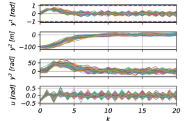
(a)

(b)

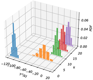
(c)

Figure 1: (a) 50 different closed-loop realization trajectories. The red-dashed lines represent the chance constraints. (b) Averaged cost (over time) of 50 different closed-loop realization trajectories. The red dashed lines represent the averaged asymptotic cost over sampling; the blue dash-dotted line represents the average asymptotic cost given by (16). (c) Histograms of the output $Y^{2}$ from 1000 closed-loop realization trajectories.

5 Conclusion

This paper has investigated data-driven stochastic output-feedback predictive control of linear time-invariant systems. We have shown that the concept of interpolating initial conditions can and should be exploited in the data-driven stochastic setting. Specifically, we have given sufficient conditions for recursive feasibility and practical stability as well as a corresponding performance bound. Numerical results illustrate the efficacy of the proposed approach. Our results, which are based on a recently proposed stochastic extension to Willems’ fundamental lemma, underpin that stochastic predictive control can be formulated in data-driven fashion. Future work will consider tailored numerical methods for real-time feasible implementation and less restrictive stability conditions.

The authors gratefully acknowledge funding by the German Research Foundation (Deutsche Forschungsgemeinschaft DFG) under project number 499435839.

References

- Allibhoy and Cortes (2020) A. Allibhoy and J. Cortes. Data-driven distributed predictive control via network optimization. In Proceedings of the 2nd Conference on Learning for Dynamics and Control, volume 120 of Proceedings of Machine Learning Research, pages 838–839. PMLR, 10–11 Jun 2020.
- Berberich et al. (2020) J. Berberich, J. Köhler, M. A. Müller, and F. Allgöwer. Data-driven model predictive control with stability and robustness guarantees. IEEE Transactions on Automatic Control, 66(4):1702–1717, 2020.
- Berberich et al. (2021) J. Berberich, J. Köhler, M. A. Müller, and F. Allgöwer. On the design of terminal ingredients for data-driven MPC. IFAC-PapersOnLine, 54(6):257–263, 2021.
- Bilgic et al. (2022) D. Bilgic, A. Koch, G. Pan, and T. Faulwasser. Toward data-driven predictive control of multi-energy distribution systems. Electric Power Systems Research, 212:108311, 2022.
- Bongard et al. (2022) J. Bongard, J. Berberich, J. Köhler, and F. Allgöwer. Robust stability analysis of a simple data-driven model predictive control approach. IEEE Transactions on Automatic Control, pages 1–1, 2022. 10.1109/TAC.2022.3163110.
- Carlet et al. (2023) P. G. Carlet, A. Favato, R. Torchio, F. Toso, S. Bolognani, and F. Dörfler. Real-time feasibility of data-driven predictive control for synchronous motor drives. IEEE Transactions on Power Electronics, 38(2):1672–1682, 2023. 10.1109/TPEL.2022.3214760.
- Coulson et al. (2019) J. Coulson, J. Lygeros, and F. Dörfler. Data-enabled predictive control: In the shallows of the DeePC. In 2019 18th European Control Conference (ECC), pages 307–312. IEEE, 2019.
- De Persis and Tesi (2020) C. De Persis and P. Tesi. Formulas for data-driven control: Stabilization, optimality, and robustness. IEEE Transactions on Automatic Control, 65(3):909–924, 2020. 10.1109/TAC.2019.2959924.
- Farina et al. (2013) M. Farina, L. Giulioni, L. Magni, and R. Scattolini. A probabilistic approach to model predictive control. In 52nd IEEE Conference on Decision and Control, pages 7734–7739, 2013. 10.1109/CDC.2013.6761117.
- Farina et al. (2015) M. Farina, L. Giulioni, L. Magni, and R. Scattolini. An approach to output-feedback MPC of stochastic linear discrete-time systems. Automatica, 55:140–149, 2015.
- Faulwasser et al. (2022) T. Faulwasser, R. Ou, G. Pan, P. Schmitz, and K. Worthmann. Behavioral theory for stochastic systems? A data-driven journey from Willems to Wiener and back again. arXiv preprint arXiv:2209.06414, 2022.
- Kantas et al. (2009) N. Kantas, J. M. Maciejowski, and A. Lecchini-Visintini. Sequential Monte Carlo for model predictive control, pages 263–273. Springer Berlin Heidelberg, Berlin, Heidelberg, 2009. ISBN 978-3-642-01094-1. 10.1007/978-3-642-01094-1_21.
- Kerz et al. (2021) S. Kerz, J. Teutsch, T. Brüdigam, D. Wollherr, and M. Leibold. Data-driven stochastic model predictive control. arXiv preprint arXiv:2112.04439, 2021.
- Koekoek and Swarttouw (1998) R. Koekoek and R. F. Swarttouw. The Askey-scheme of hypergeometric orthogonal polynomials and its q-analogue. Technical Report 98-17, Department of Technical Mathematics and Informatics, Delft University of Technology, Delft, The Netherlands, 1998.
- Köhler and Zeilinger (2022) J. Köhler and M. N. Zeilinger. Recursively feasible stochastic predictive control using an interpolating initial state constraint. IEEE Control Systems Letters, 2022.
- Lefebvre (2021) T. Lefebvre. On moment estimation from polynomial chaos expansion models. IEEE Control Systems Letters, 5(5):1519–1524, 2021. 10.1109/LCSYS.2020.3040851.
- Lian and Jones (2021) Y. Lian and C. N. Jones. Nonlinear data-enabled prediction and control. In Proceedings of the 3rd Conference on Learning for Dynamics and Control, volume 144 of Proceedings of Machine Learning Research, pages 523–534. PMLR, 07 – 08 June 2021.
- Maciejowski (2002) J. M. Maciejowski. Predictive Control with Constraints. Pearson Education, 2002.
- Markovsky and Dörfler (2021) I. Markovsky and F. Dörfler. Behavioral systems theory in data-driven analysis, signal processing, and control. Annual Reviews in Control, 52:42–64, 2021. ISSN 1367-5788.
- Mesbah et al. (2014) A. Mesbah, S. Streif, R. Findeisen, and R. D. Braatz. Stochastic nonlinear model predictive control with probabilistic constraints. In 2014 American Control Conference, pages 2413–2419, 2014. 10.1109/ACC.2014.6858851.
- Mühlpfordt et al. (2018) T. Mühlpfordt, R. Findeisen, V. Hagenmeyer, and T. Faulwasser. Comments on truncation errors for polynomial chaos expansions. IEEE Control Systems Letters, 2(1):169–174, 2018. 10.1109/LCSYS.2017.2778138.
- Ou et al. (2021) R. Ou, M. H. Baumann, L. Grüne, and T. Faulwasser. A simulation study on turnpikes in stochastic LQ optimal control. IFAC-PapersOnLine, 54(3):516–521, 2021. https://doi.org/10.1016/j.ifacol.2021.08.294. 16th IFAC Symposium on Advanced Control of Chemical Processes ADCHEM 2021.
- Pan et al. (2022a) G. Pan, R. Ou, and T. Faulwasser. On data-driven stochastic output-feedback predictive control. arXiv preprint, 2022a.
- Pan et al. (2022b) G. Pan, R. Ou, and T. Faulwasser. On a stochastic fundamental lemma and its use for data-driven optimal control. IEEE Transactions on Automatic Control, accepted for publication, 2022b. arXiv preprint arXiv:2111.13636.
- Pan et al. (2022c) G. Pan, R. Ou, and T. Faulwasser. Towards data-driven stochastic predictive control. International Journal of Robust and Nonlinear Control, 2022c. Submitted.
- Paulson et al. (2014) J. A. Paulson, A. Mesbah, S. Streif, R. Findeisen, and R. D. Braatz. Fast stochastic model predictive control of high-dimensional systems. In 53rd IEEE Conference on Decision and Control, pages 2802–2809, 2014. 10.1109/CDC.2014.7039819.
- Sadamoto (2022) T. Sadamoto. On equivalence of data informativity for identification and data-driven control of partially observable systems. IEEE Transactions on Automatic Control, pages 1–8, 2022. 10.1109/TAC.2022.3202082.
- Schildbach et al. (2014) G. Schildbach, L. Fagiano, C. Frei, and M. Morari. The scenario approach for stochastic model predictive control with bounds on closed-loop constraint violations. Automatica, 50(12):3009–3018, 2014. ISSN 0005-1098.
- Schlüter and Allgöwer (2022) H. Schlüter and F. Allgöwer. Stochastic model predictive control using initial state optimization. arXiv preprint arXiv:2203.01844, 2022.
- Sullivan (2015) T. J. Sullivan. Introduction to Uncertainty Quantification, volume 63. Springer, 2015.
- Tempo et al. (2013) R. Tempo, G. Calafiore, and F. Dabbene. Randomized algorithms for analysis and control of uncertain systems: with applications. Springer London, 2 edition, 2013.
- Wang et al. (2022a) J. Wang, Y. Zheng, K. Li, and Q. Xu. DeeP-LCC: Data-enabled predictive leading cruise control in mixed traffic flow. arXiv preprint arXiv:2203.10639, 2022a.
- Wang et al. (2022b) Y. Wang, C. Shang, and D. Huang. Data-driven control of stochastic systems: An innovation estimation approach. arXiv preprint arXiv:2209.08995, 2022b.
- Wiener (1938) N. Wiener. The homogeneous chaos. American Journal of Mathematics, pages 897–936, 1938.
- Willems et al. (2005) J. C. Willems, P. Rapisarda, I. Markovsky, and B. L. De Moor. A note on persistency of excitation. Systems & Control Letters, 54(4):325–329, 2005. https://doi.org/10.1016/j.sysconle.2004.09.003.
- Wu (2022) L. Wu. Equivalence of SS-based MPC and ARX-based MPC. arXiv preprint arXiv:2209.00107, 2022.
- Xiu and Karniadakis (2002) D. Xiu and G. E. Karniadakis. The Wiener–Askey polynomial chaos for stochastic differential equations. SIAM Journal on Scientific Computing, 24(2):619–644, 2002. 10.1137/S1064827501387826.
- Yang and Li (2015) H. Yang and S. Li. A data-driven predictive controller design based on reduced Hankel matrix. In 2015 10th Asian Control Conference (ASCC), pages 1–7, 2015. 10.1109/ASCC.2015.7244723.