Ungeneralizable Contextual Logistic Bandit in Credit Scoring

Abstract

The application of reinforcement learning in credit scoring has created a unique setting for contextual logistic bandit that does not conform to the usual exploration-exploitation tradeoff but rather favors exploration-free algorithms. Through sufficient randomness in a pool of observable contexts, the reinforcement learning agent can simultaneously exploit an action with the highest reward while still learning more about the structure governing that environment. Thus, it is the case that greedy algorithms consistently outperform algorithms with efficient exploration, such as Thompson sampling. However, in a more pragmatic scenario in credit scoring, lenders can, to a degree, classify each borrower as a separate group, and learning about the characteristics of each group does not infer any information to another group. Through extensive simulations, we show that Thompson sampling dominates over greedy algorithms given enough timesteps which increase with the complexity of underlying features.

Keywords: Contextual Logistic Bandits, Credit Scoring, Thompson Sampling, Natural Exploration, Ungeneralizable Contexts

1 Introduction

Credit scoring has been a staple of machine learning applications for decades, having been applied both naive and complex algorithms [Dastile et al., 2020]; nonetheless, this seemingly trivial problems have become more and more prevalent and crucial to the financial sector as businesses have adapted themselves to the data-driven platforms and have started to accumulate a sizeable dataset which can be turned into insight and, eventually, profitability. This success is, however, based on several unwarranted assumptions, one of which is how samples are labelled. Normally, the process of model construction and implementaton is thought to be separate entities, which has led to underestimation of intrinsic cost of creating a machine learning system for credit scoring since the cost of data labelling is astronomical in this situation.

Consider the paradigm to learn the process of loan approval for a short-term loan of one year. The lender has a choice to approve or deny the request for the loan from each individual while considering from a narrow list of visible features such as age, credit history, occupation, income, etc. Only by approving the loan to the borrowers could the lender know whether these customers would repay the loan or not, thus creating a costly loop, in terms of monetary value and time, to obtain the labels. However, this process often is ignored or dismissed when the lender tries to create an intelligence system through learning models. Thus, we primarily concern with the amalgamation between two processes and making this model as realsitic and cost-saving as possible.

This study extends the scope of framing the credit scoring as logistic bandit [Visantavarakul and Kiatsupaibul, 2022] by incorporating the context which could be thought of as distinct characteristics that discriminate each customer segment from one another. Furthermore, it is possible that the real-world cluster would share similarities between groups, hence the context features in our study are simulated as unit vectors which are orthogonal to each other and form an identity matrix when being stacked in columns.

Therefore, the framework used in this study is the contextual logistic bandit framework. The brief settings are as follows: there are a certain number of borrowers who apply for loans, and a reinforcement learning agent has to select a small number of borrowers whom credit would be granted to. While this process is prevalent in the practicality, it is considered to be a greedy algorithm thanks to the fact that lenders only take into an account the reward of the current approval process without prudently considering about the future. As mentioned in [Sutton and Barto, 2018], this simple algorithm is sub-optimal and incurs linear regret since it commits too early to any action which has the highest reward from taking action in an environment for only once.

A superior alternative to greedy algorithms in most situations is $\epsilon$-greedy algorithm; however, this exploration strategy is still not efficient since it will continue to select sub-optimal actions even after an optimal action has been discovered. Finally, ones that people in the field consider to be the gold standard of modern reiforcement learning are the strategies of Optimism under uncertainty (OFU), a group of strategies that adopt almost the same idea of being sanguine for an action that an agent is uncertain about, some of the most well-known algorithms in this group are, such as, Upper Confidence Bound (UCB) and Thompson sampling. The latter performs an efficient exploration by sampling the model estimates from posterior distribution that is being constantly updated after an agent has observed the outcomes and rewards, this algorithm can be shown to outperform the $\epsilon$-greedy in most environments [Russo et al., 2018, Chapelle and Li, 2011] and was proven theoretically to be optimal [Agrawal and Goyal, 2013, 2017].

Under realistic scenario of credit scoring, we regard the borrower characteristics as underlying features which then could be used to construct an explicit relationship between features and observations $y=f(\beta^{T}X)$. In our case, a rather simple case of whether borrowers are going to repay the loan or not is considered such that $O_{t+1}=\textrm{Bern}(p)$ where $p=logistic\left(\beta^{T}X_{t}\right)$ and $\textrm{Bern}(p)$ is to simulate from Bernoulli distribution with positive probability of $p$; therefore, the probability of the outcomes follow logistic function and dovetails with the formulation of logistic bandits. This study extends the previous study on the same topic [Visantavarakul and Kiatsupaibul, 2022] which proposed and showed that greedy algorithms could, surprisingly, outperform Thompson sampling whenever there is enough randomness in observed contexts which eliminates the need for exploration. This finding may discourage the future study of efficient exploration in the multi-armed bandits environment with, so-called, natural exploration. Therefore, our work aims to show that, under some realistic constraint in context features, Thompson sampling can outperform greedy algorithm with an ease.

The organization is as follows. In Section 2, problem formulation including the structure of the multi-armed bandit environment and algorithms of greedy and Thompson sampling is defined. In Section 3, the results from simulations are presented and discussed. Lastly, in Section 4, a conclusion is provided

2 Problem Formulation

In this study, we formulate the problem of credit scoring as contextual logistic bandit where, at timestep $t$, there are $N$ borrowers or samples, and each sample is regarded as an action $\{A_{t};A_{t}=1,...,N\}$. Likewise, there are $M$ contexts which alter how action features react to ground truth parameters $\theta$. This context is assigned to each and every sample in the equal proportion such that there will be approximately $\lfloor\frac{N}{M}\rfloor$ samples in each context $m$. For our problem specific setting, we consider two cases of feature generation: renewal and non-renewal. Non-renewal variant conforms to the traditional multi-armed bandits where every action remains static throughout many simulation rounds, whereas renewal variant samples a new set of action at the end of every timestep. Furthermore, we examine another two cases: first, an agent can choose to take only one action per timestep and, second, a batch training that allows an agent to select $k$ actions per timestep.

This environment is simulated together with a ground truth parameter matrix $\theta\in\mathbb{R}^{d\times m}$ drawn from a standard multivariate normal distribution $\mathcal{N}(0,I)$ which does not change with timestep until the end of a simulation round, action feature vectors $\{\phi_{n}\in\mathbb{R}^{d};n=1,...,N\}$, and context feature vectors $\{\psi_{m}\in\mathbb{R}^{m};m=1,...,M\}$. In our case, context feature vectors $\psi_{m}$ are unit vector, which can be stacked as column vectors, resulting in identity matrix. At timestep $t$, action features $\phi_{A_{t}}$ are sampled identically and independently (iid) from a standard multivariate normal distribution with an identity covariance matrix $I$. Additionally, the parameter matrix $\theta$, action feature vector $\phi$, and context feature vector $\psi$ are independent. The non-default probability of each borrower follows the function $\text{I\kern-1.49994ptP}(O_{i,t+1}=1)=\textrm{logistic}(\phi_{i}^{T}\theta\psi_{m})$ where $\textrm{logistic}(x)=\frac{1}{1+e^{-x}}$ and $m$ is a context as specified by the environment. The observation $O_{i,t+1}$ is a sample from $\textrm{Bern}(\textrm{logistic}(\phi_{A_{t}}^{T}\theta\psi_{m}))$ where 1 denotes the event that borrower does not default and 0 denotes the opposite.

Finally, since we allow the agent to choose $k\ll N$ actions from the action set, our posterior update rule is to perform $k$ sequential maximum likelihood update without taking an order into consideration which will accelerate the training process since it is equivalent to learning from $kT$ samples as opposed to only $T$ samples.

The environment $\varepsilon$ consists of an action set, a context set, an observation set, and observation probabilities such that $\varepsilon=(\mathcal{A},\mathcal{C},\mathcal{O},\text{I\kern-1.49994ptP})$ as follows

1. action set: $\mathcal{A}=\{1,2,...,N\}$

2. context set: $\mathcal{C}=\{1,2,...,M\}$

3. observation set: $\mathcal{O}=\{0,1\}^{k}$

4. observation probabilities: given history $H_{t}$, context $C_{t}$, and action $A_{t}$

   $$\text{I\kern-1.49994ptP}(O_{t+1}|H_{t},A_{t})=\prod_{i=1}^{k}\text{I\kern-1.49994ptP}(O_{i,t+1}|H_{t},A_{t})$$ (1)

   $$\text{I\kern-1.49994ptP}(O_{i,t+1}|H_{t},A_{t},C_{t},\varepsilon)=\begin{cases}\frac{\exp(\phi_{A_{t}}^{T}\theta\psi_{C_{t}})}{1+\exp(\phi_{A_{t}}^{T}\theta\psi_{C_{t}})}&\text{; $O_{i,t+1}=1$}\\ \frac{1}{1+\exp(\phi_{A_{t}}^{T}\theta\psi_{C_{t}})}&\text{; $O_{i,t+1}=0$}\end{cases}$$ (2)

The environment is characterized by the ground truth parameter $\theta$, which is utilized to generate an observation $O_{t+1}$ according to the non-default probability calculated using (1) and (2). However, the agent does not directly observe parameters $\theta$ but can observe the action feature of each borrower $\phi_{i,t}$ and context feature $\psi_{C_{t}}$ of each and every context.

Instead, the agent estimates $\hat{\theta}_{t}$ at timestep $t$, which is utilized to infer non-default probabilities of all borrowers, and the agent would grant loans to $k$ borrowers with the $k$-highest inferred non-default probabilities. Then, let $\accentset{\rightharpoonup}{A}_{t}\in\mathbb{N}^{k}$ be the set containing selected actions. Unlike traditional multi-armed bandit agents, contextual logistic bandit adopts the idea of generalization across actions which emphasize on the ability to generalize the information from one action to other actions in the way that, learning from action ${a;a\in\mathcal{A}}$ would help improve the estimation of other actions ${A_{t};A_{t}\neq a\in\mathcal{A}}$.

This study conducts similar experiments as previously done in the preceding study of Visantavarakul and Kiatsupaibul [2022]; however, the contextual environment here is more complex. While there is generalization across action feature, the context feature is designed to prevent the flow of information from one contexts to any other, in the other words, contexts are ungeneralizable. That is, if $M=3$,

$$\psi=I_{3}=\begin{bmatrix}1&0&0\\ 0&1&0\\ 0&0&1\end{bmatrix}$$

The context feature, which is a unit vector, is randomly assinged to each action but with equal proportion in every timestep. For every simulation trial, context features $\psi$ remains unchanged, but the environment will sample one context feature to be paired with each action. Thus, we name this new list of context features action-context vector $\widetilde{\psi}_{t}\in\mathbb{R}^{M\times N}$. Furthermore, to simplify the process of keeping track of history $H_{t}$, we combine $\phi_{A_{t}}$ and $\psi_{A_{t}}$ through a simple operation

$$emb_{A_{t}}=\psi_{A_{t}}^{T}\left(I_{M}\otimes\phi_{A_{t}}\right)\forall A_{t}\in\mathcal{A}$$ (3)

With embedding $emb_{A_{t}}\in\mathbb{R}^{1\times d}$, we could vectorize estimated paramter matrix $\hat{\theta}_{t}$ into a column vector and, then, uses any modules that have solver for logistic regression. This embedding is interchangable with terminology of input $X_{t}$ in supervised learning and could be used as an update to history $H_{t}$.

We conducted extensive simulations on multiple sets of hyperparameters to evaluate how each algorithm would perform under contextual logistic bandit framework. The number of timestep differs depending on how complex the environment, but is set at 500 per simulation round as a default. The performance of each agent is averaged on 100 trials. The algorithms include greedy algorithm and Thompson sampling with two variants of posterior approximations: Laplace approximation and Langevin Monte-carlo Markov chain [Xu et al., 2022].

2.1 Greedy Alogrithm

The greedy algorithm uses all of information the agent has collected to select what it perceives as an optimal action. This is the algorithm used in a traditional credit scoring, where the model estimation is considered separately from loan underwriting. The main advantage is that the agent fully uses the information collected in the history, called an exploitation. However, the drawback is that the greedy algorithm commits too early to just a few observations the agent has collected. In other words, the algorithm lacks an exploration. An exploration is when an action with limited information is chosen in order to improve the estimate of how good the action actually is.

There is a significant tradeoff between exploration and exploitation since, in traditional setting, they could not be conduceted simultaneously, an agent needs to choose between reaping the highest expected reward from the action that the agent esimates to be optimal (exploitation) or searching for possibly better action that would yield higher expected reward (exploration) which sacrifices a chance to choose an action optimally. Therefore, according to Sutton and Barto [2018], Russo et al. [2018], it is commonly believed that the greedy algorithm achieves sub-optimal performance due to the lack of exploration.

The setting is that an agent starts with prior of a standard normal distribution, and the estimated parameter $\hat{\theta}_{0}$ is updated through the likelihood of logistic function as follows.

1. prior distribution of $\theta$: $\hat{\theta}_{0}\sim\mathcal{N}(0,I_{d\cdot m})$

2. likelihood of $\hat{\theta}$:

   $$f(\hat{\theta};\phi_{1},...,\phi_{N},\psi_{1},...,\psi_{N},O_{1},...,O_{N})=$$

   $$\prod_{i=1}^{N}\left(\frac{\exp(\phi_{i}^{T}\hat{\theta}\psi_{i})}{1+\exp(\phi_{i}^{T}\hat{\theta}\psi_{i})}\right)^{O_{i}}\left(\frac{1}{1+\exp(\phi_{i}^{T}\hat{\theta}\psi_{i})}\right)^{(1-O_{i})}$$ (4)

To exploit the information that the agent has already collected, the agent has to find $\hat{\theta}$ that maximizes the posterior, proportional to the normal prior multiplied by the logistic likelihood (2). Finding such $\hat{\theta}$ is equivalent to fitting $\hat{\theta}$ to the logistic regression with L2 regularization. The implementation details of the greedy is specified in Algorithm 1.

Algorithm 1 Greedy Algorithm

Input: number of actions N, number of selected actions k,
    Likelihood function $\mathcal{L}()$

1:  $X=\varnothing,Y=\varnothing,init=\textrm{True}$

2:  for $t=0,1,...$ do

3:     if $init=\textrm{True}$ then

4:        Choose $k$ actions randomly from $\{1,2,...,N\}$ into $\accentset{\rightharpoonup}{A}_{t}$

5:     else

6:        Compute $emb_{A_{t}}=\psi_{A_{t}}^{T}\left(I_{M}\otimes\phi_{A_{t}}\right)\forall A_{t}\in\mathcal{A}$

7:        $\accentset{\rightharpoonup}{A}_{t}=\operatorname*{arg\,max}_{\accentset{\rightharpoonup}{A}_{t}\subseteq A,\lVert\accentset{\rightharpoonup}{A}_{t}\rVert=k}\frac{\exp\left(emb_{A_{t}}\cdot vec\left(\widehat{\theta}_{t}\right)\right)}{1+\exp\left(emb_{A_{t}}\cdot vec\left(\widehat{\theta}_{t}\right)\right)}$

8:     end if

9:     Play arms $\accentset{\rightharpoonup}{A}_{t}$ and observe observations $O_{\accentset{\rightharpoonup}{A}_{t}}$ and rewards $r_{t}$

10:     Append $X\leftarrow X\cup\{emb_{a_{1},t},...,emb_{a_{k},t}\};a_{1},...,a_{k}\in\accentset{\rightharpoonup}{A}_{t}$

11:     Append $Y\leftarrow Y\cup\{O_{a_{1},t+1},...,O_{a_{k},t+1}\};a_{1},...,a_{k}\in\accentset{\rightharpoonup}{A}_{t}$

12:     if $init=\textrm{True}\cap\{0,1\}\subseteq Y$ then

13:        $init=\textrm{False}$

14:     end if

15:     if $init=\textrm{False}$ then

16:        $\widehat{\theta}_{t}=\operatorname*{arg\,max}_{\theta}\mathcal{L}(\theta|X,Y)=\operatorname*{arg\,max}_{\theta}\prod\limits_{\tau=0}^{k*(t-1)}\text{I\kern-1.49994ptP}\left(Y_{\tau+1}|X_{\tau},\theta\right)\mathcal{L}(\theta)$

17:     end if

18:  end for

2.2 Thompson sampling

According to Russo et al. [2018], Thompson sampling algorithm is a reinforcement learning algorithm that performs an efficient exploration. Prior to selecting an action, the algorithm samples a parameter vector $\hat{\theta}$ from the posterior distribution, and its value is used to select the action that maximizes the estimated expected reward. In the context of credit scoring and underwriting, the outcomes of $k$ selected borrowers are used to update the posterior distribution of $\hat{\theta}$ via Bayes’ rule. In contrast to the greedy algorithm that lacks an exploration in the feature space of $\hat{\theta}$, Thompson sampling relies on efficient exploration. Whereas the $\epsilon$-greedy algorithm explores the environment by choosing one of all possible actions randomly, Thompson sampling chooses an action that agent has limited information about with a high probability, thus would not select an action which is certainly inferior to others. [Russo et al., 2018] The implementation details of Thompson sampling is specified in Algorithm 2.

However, if the posterior distribution is not a conjugate of the prior distribution, an exact Bayesian inference would be too complicated [Russo et al., 2018] or even be computationally intractable. In the logistic bandit framework, the functional form of logistic regression results in a computationally intractable posterior, which makes the application of Thompson sampling in this framework difficult to tackle [Dumitrascu et al., 2018]. To address this problem, an approximation method will be used. This study considers two variants of posterior approximations: Laplace approximation and Langevin MCMC.

Algorithm 2 Thompson sampling

Input: number of actions N, number of selected actions k

1:  $X=\varnothing,Y=\varnothing,init=\textrm{True}$

2:  Initialize prior $P_{0}=\mathcal{N}(\mu,\Sigma)$

3:  for $t=0,1,...$ do

4:     if $init=\textrm{True}$ then

5:        Choose $k$ actions randomly from $\{1,2,...,N\}$ into $\accentset{\rightharpoonup}{A}_{t}$

6:     else

7:        Sample $\widehat{\theta}_{t}\sim\text{I\kern-1.49994ptP}(\theta|X,Y)$

8:        Compute $emb_{A_{t}}=\psi_{A_{t}}^{T}\left(I_{M}\otimes\phi_{A_{t}}\right)\forall A_{t}\in\mathcal{A}$

9:        $\accentset{\rightharpoonup}{A}_{t}=\operatorname*{arg\,max}_{\accentset{\rightharpoonup}{A}_{t}\subseteq A,\lVert\accentset{\rightharpoonup}{A}_{t}\rVert=k}\frac{\exp\left(emb_{A_{t}}\cdot vec\left(\widehat{\theta}_{t}\right)\right)}{1+\exp\left(emb_{A_{t}}\cdot vec\left(\widehat{\theta}_{t}\right)\right)}$

10:     end if

11:     Play arms $\accentset{\rightharpoonup}{A}_{t}$ and observe observations $O_{\accentset{\rightharpoonup}{A}_{t}}$ and rewards $r_{t}$

12:     Append $X\leftarrow X\cup\{emb_{a_{1},t},...,emb_{a_{k},t}\};a_{1},...,a_{k}\in\accentset{\rightharpoonup}{A}_{t}$

13:     Append $Y\leftarrow Y\cup\{O_{a_{1},t+1},...,O_{a_{k},t+1}\};a_{1},...,a_{k}\in\accentset{\rightharpoonup}{A}_{t}$

14:     if $init=\textrm{True}\cap\{0,1\}\subseteq Y$ then

15:        $init=\textrm{False}$

16:     end if

17:     if $init=\textrm{False}$ then

18:        Update $\text{I\kern-1.49994ptP}(\theta|X,Y)$ according to Bayes’ rule

19:     end if

20:  end for

2.2.1 Thompson sampling: Laplace Approximation

Laplace approximation is a technique to approximate any function that has a well-behaved unimodal. Since the desired posterior is the likelihood function of logistic regression loss function, it is certain that there is only one global maximum or global minimum depending on the sign of likelihood function. Thus, Laplace approximation is usually adopted in Bayesian logistics regression and will be implemented in our study as well.

It could be said that Laplace approximation tries to set the mode of its Gaussian approximation to the mode of posterior distribution and attempts to match the shape of its density. In the other word, we approximate $\text{I\kern-1.49994ptP}(\theta|H_{t})$ by the best-fit multivariate normal distribution $\mathcal{N}(\mu_{t},\Sigma_{t})$ where $\mu_{t}$ is solved as optimization problem in logistic regression and $\Sigma_{t}$ is the inverse of Hessian matrix of $\mathcal{L}(\theta,H_{t})$ at $\mu_{t}$.

We then sample from this approximated posterior distribution to be used as esitmated parameters in the next timestep, update the approximation from the observations, and iteratively follow this process until the end of simulation round.

The implementation details of Laplace approximation is specified in Algorithm 3.

Algorithm 3 Laplace Approximation Thompson sampling

Input: number of actions N, number of selected actions k,
    Likelihood function $\mathcal{L}()$, Hessian function $H()$

1:  $X=\varnothing,Y=\varnothing,init=\textrm{True}$

2:  Initialize prior $P_{0}=\mathcal{N}(\mu,\Sigma)$

3:  for $t=0,1,...$ do

4:     if $init=\textrm{True}$ then

5:        Choose $k$ actions randomly from $\{1,2,...,N\}$ into $\accentset{\rightharpoonup}{A}_{t}$

6:     else

7:        Set $\tilde{P}_{t}(\theta)=\mathcal{N}(\mu_{t},\Sigma_{t})$

8:        Sample $\widehat{\theta}_{t}\sim\tilde{P}_{t}(\theta)$

9:        Compute $emb_{A_{t}}=\psi_{A_{t}}^{T}\left(I_{M}\otimes\phi_{A_{t}}\right)\forall A_{t}\in\mathcal{A}$

10:        $\accentset{\rightharpoonup}{A}_{t}=\operatorname*{arg\,max}_{\accentset{\rightharpoonup}{A}_{t}\subseteq A,\lVert\accentset{\rightharpoonup}{A}_{t}\rVert=k}\frac{\exp\left(emb_{A_{t}}\cdot vec\left(\widehat{\theta}_{t}\right)\right)}{1+\exp\left(emb_{A_{t}}\cdot vec\left(\widehat{\theta}_{t}\right)\right)}$

11:     end if

12:     Play arms $\accentset{\rightharpoonup}{A}_{t}$ and observe observations $O_{\accentset{\rightharpoonup}{A}_{t}}$ and rewards $r_{t}$

13:     Append $X\leftarrow X\cup\{emb_{a_{1},t},...,emb_{a_{k},t}\};a_{1},...,a_{k}\in\accentset{\rightharpoonup}{A}_{t}$

14:     Append $Y\leftarrow Y\cup\{O_{a_{1},t+1},...,O_{a_{k},t+1}\};a_{1},...,a_{k}\in\accentset{\rightharpoonup}{A}_{t}$

15:     if $init=\textrm{True}\cap\{0,1\}\subseteq Y$ then

16:        $init=\textrm{False}$

17:     end if

18:     if $init=\textrm{False}$ then

19:        $\mu_{t+1}=\operatorname*{arg\,max}_{\theta}\mathcal{L}(\theta|X,Y)=\operatorname*{arg\,max}_{\theta}\prod\limits_{\tau=0}^{k*(t-1)}[\text{I\kern-1.49994ptP}\left(Y_{\tau+1}|X_{\tau},\theta\right)]\mathcal{L}(\theta)$

20:        $\Sigma_{t+1}=H^{-1}(\theta;X)$

21:     end if

22:  end for

2.2.2 Thompson sampling: Langevin Monto-Carlo Markov chain

Since Laplace approximation requires the inverse of Hessian matrix which scale with the number of features, it may become computationally intractable from more complicated model such as neural network. Moreover, the posterior distribution may not retain the bell-shape curve that could be appropriately approximated by Gaussian distribution.

Another alternative which is prevalent in the field of Bayesian posterior approximation is Langevin MCMC. However, this option still has intrinsic problems which prevent the practitioners from widely adopting this method which is the fact that it requires a starting point for Monte-carlo Markov chain, and its performance depends on how well this point is selected. Therefore, we adopted the novel algorithm of Langevin Monte Carlo Thompson Sampling (LMC-TS) [Xu et al., 2022] that does not require a starting point and involves only sufficient simple noisy gradient updates. In our experiments, it had exhibited similar behaviors but converged faster than the Thompson sampling agent which uses Laplace approximation.

The implementation of LMC-TS is specified in Algorithm 4 with the step size $\eta=0.01$ and inverse temperature parameters $\beta=2$.

Algorithm 4 Langevin Monte Carlo Thompson sampling (LMC-TS)

Input: number of actions N, number of selected actions k,
Loss function $L_{t}(\theta)$, Initial step size $\boldsymbol{\eta_{0}}$, temperature parameter $\boldsymbol{\beta}$

1:  $X=\varnothing,Y=\varnothing,init=\textrm{True}$

2:  for $t=0,1,...$ do

3:     if $init=\textrm{True}$ then

4:        Choose $k$ actions randomly from $\{1,2,...,N\}$ into $\accentset{\rightharpoonup}{A}_{t}$

5:     else

6:        $\theta_{t,0}=\theta_{t-1,K_{t-1}}$ and $\eta_{t}=\frac{\eta_{0}}{t+1}$

7:        Compute $emb_{A_{t}}=\psi_{A_{t}}^{T}\left(I_{M}\otimes\phi_{A_{t}}\right)\forall A_{t}\in\mathcal{A}$

8:        for $k=1,...,K_{t}$ do

9:           sample a standard normal vector $\epsilon_{t,k}\sim\mathcal{N}(0,I)$

10:           $\theta_{t,k}=\theta_{t,k-1}-\eta_{t}\nabla L_{t}(\theta_{t,k-1})+\sqrt{2\eta_{t}\beta_{t}^{-1}\epsilon_{t,k}}$

11:        end for

12:        $\accentset{\rightharpoonup}{A}_{t}=\operatorname*{arg\,max}_{\accentset{\rightharpoonup}{A}_{t}\subseteq A,\lVert\accentset{\rightharpoonup}{A}_{t}\rVert=k}\frac{\exp\left(emb_{A_{t}}\cdot vec\left(\widehat{\theta}_{t}\right)\right)}{1+\exp\left(emb_{A_{t}}\cdot vec\left(\widehat{\theta}_{t}\right)\right)}$

13:     end if

14:     Play arms $\accentset{\rightharpoonup}{A}_{t}$ and observe observations $O_{\accentset{\rightharpoonup}{A}_{t}}$ and rewards $r_{t}$

15:     Append $X\leftarrow X\cup\{emb_{a_{1},t},...,emb_{a_{k},t}\};a_{1},...,a_{k}\in\accentset{\rightharpoonup}{A}_{t}$

16:     Append $Y\leftarrow Y\cup\{O_{a_{1},t+1},...,O_{a_{k},t+1}\};a_{1},...,a_{k}\in\accentset{\rightharpoonup}{A}_{t}$

17:     if $init=\textrm{True}\cap\{0,1\}\subseteq Y$ then

18:        $init=\textrm{False}$

19:     end if

20:  end for

3 Results and Discussions

Firstly, aforementioned algorithms are evaluated on the low-dimensional samples with only two features and, at each timestep, the pool of actions remains unchanged throughout each simulation round (Figure 1), where the performance of each algorithm is expressed through the plots of regrets and rewards, including the cumulative regrets and rewards since the magnitude of differences is subtle. The reward of 0.2 is given for when the observation $O_{t+1}$ is 1; likewise, the reward of -1 is given as the outcome $O_{t+1}$ is 0. Regret is calculated as the discrepancy between the maximum expected reward over all possible actions and the expeected rewards from taking a certain action. Both of these values are reflected in the plot below.

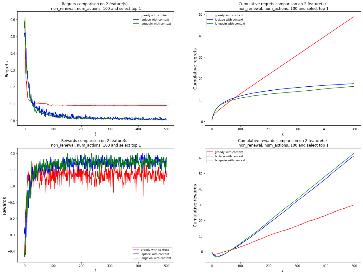
Figure 1: Performance comparison in 2-feature selecting top 1 without renewal setting

The performances of each algorithm under the setting with two-dimension features and non-renewal are illustrated in Figure 1. This setting is almost identical to the traditional mutli-armed bandit problems as the agent could select only a single action per period and the pool of action is fixed. The ground-truth parameter $\theta$ is sampled from $\mathcal{N}(0,I)$. From Figure 1, the greedy algorithm performs worst since it has the lowest cumulative reward and the highest cumulative regret at the last timestep, while Thompson sampling outperforms the former by a significant margin.

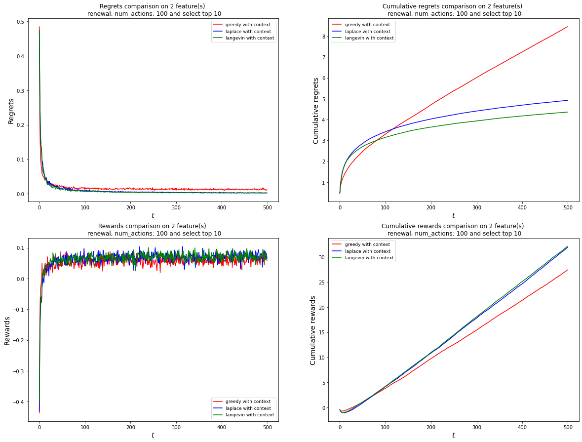
Figure 2: Performance comparison in 2-feature selecting top 10 with renewal setting

As an application to credit scoring, lender acts as an agent to grant the loans to multiple borrowers at each period, and these borrowers would not be exactly the same group with the same characteristics but constantly change from one timestep to another. Therefore, our complicated setting will consider 10 borrowers at once, that is, $k=10$ and the action features, including action-context vectors are picked randomly from an unknown pool in the environment. The results are shown in Figure 2. Even with renewal in the action set, Thompson sampling still accumulated less regrets and more rewards over the timestep with greedy algorithm taking a short lead about the first hundredth steps, showing the effect of unit context features that prohibit the flow of information across different contexts. In the previous work [Bastani et al., 2020], it is obvious that greedy algorithm performed much better than Thompson sampling since it has enough information to infer the correct parameters without the need to explore; however, when we added this type of context feature into the environment, relying only on natural exploration is no longer adequate to learn about optimal actions. This is conspicuously shown in Figure 2.

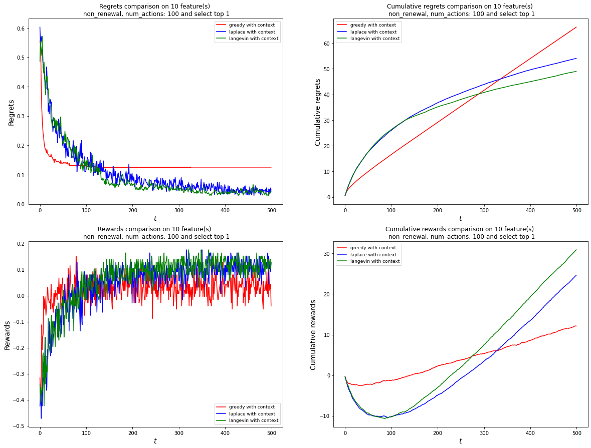
Figure 3: Performance comparison in 10-feature selecting top 1 without renewal setting

For the higher dimensionality, this study follows Visantavarakul and Kiatsupaibul [2022] by adjusting the signal-to-noise ratio with the adjustment coefficient $\sqrt{2/d}$ to make the difference in the number of features negligible. Consider the case when the environment is governed by 10-dimension action features which is more complicated than the case before, and it will take more time for the model to learn as evidenced by, without natural exploration mechanism, both greedy algorithm and Thompson sampling having a negative rewards for the time being before recovering, especially for Thompson sampling which takes around 100 timesteps before the line starts turning positive. Overall, from Figure 3 although greedy algorithm has a lower cumulative regret for approximately first 300 timesteps, Thompson sampling still achieves much higher rewards and lower regrets. Notice that Langevin MCMC Thompson sampling yields lower regrets and considerably higher rewards compared to Laplace approximation variant of Thompson sampling.

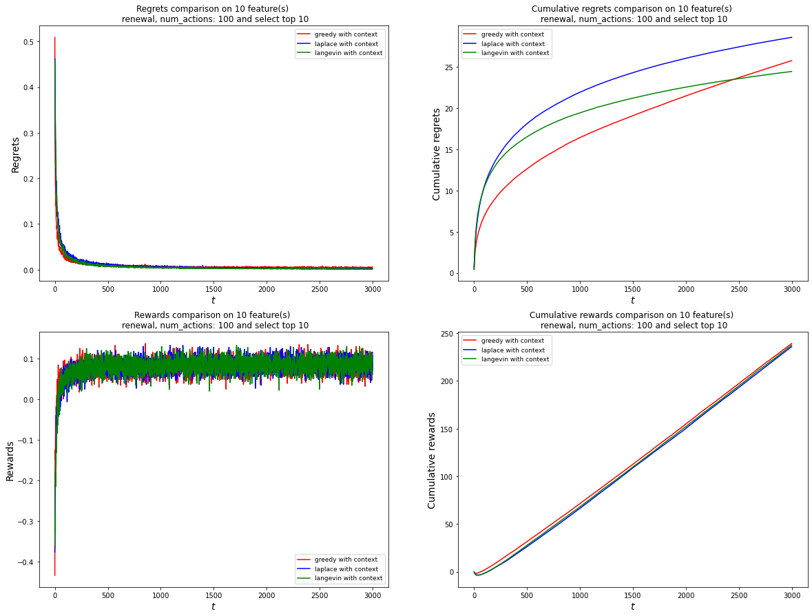
Figure 4: Performance comparison in 10-feature selecting top 10 with renewal setting

With an addition of natural exploration mechanism (renewal) and multiple occasions for an agent to take actions (selecting top 10), greedy algorithm has shown a sign of being able to learn the convoluted environment; nevertheless, Thompson sampling still performs better in the later stage as can be seen in Figure 4. However, it takes around 3,000 steps before the regret of Langevin MCMC Thompson sampling can overcome that of greedy algorithm, which might be unrealistic to be considered in practice. Lastly, even though a figure that represents the regret of Laplace approximation is still higher than that of greedy algorithm, it has started to plateau and would soon outstrip that of greedy algorithm.

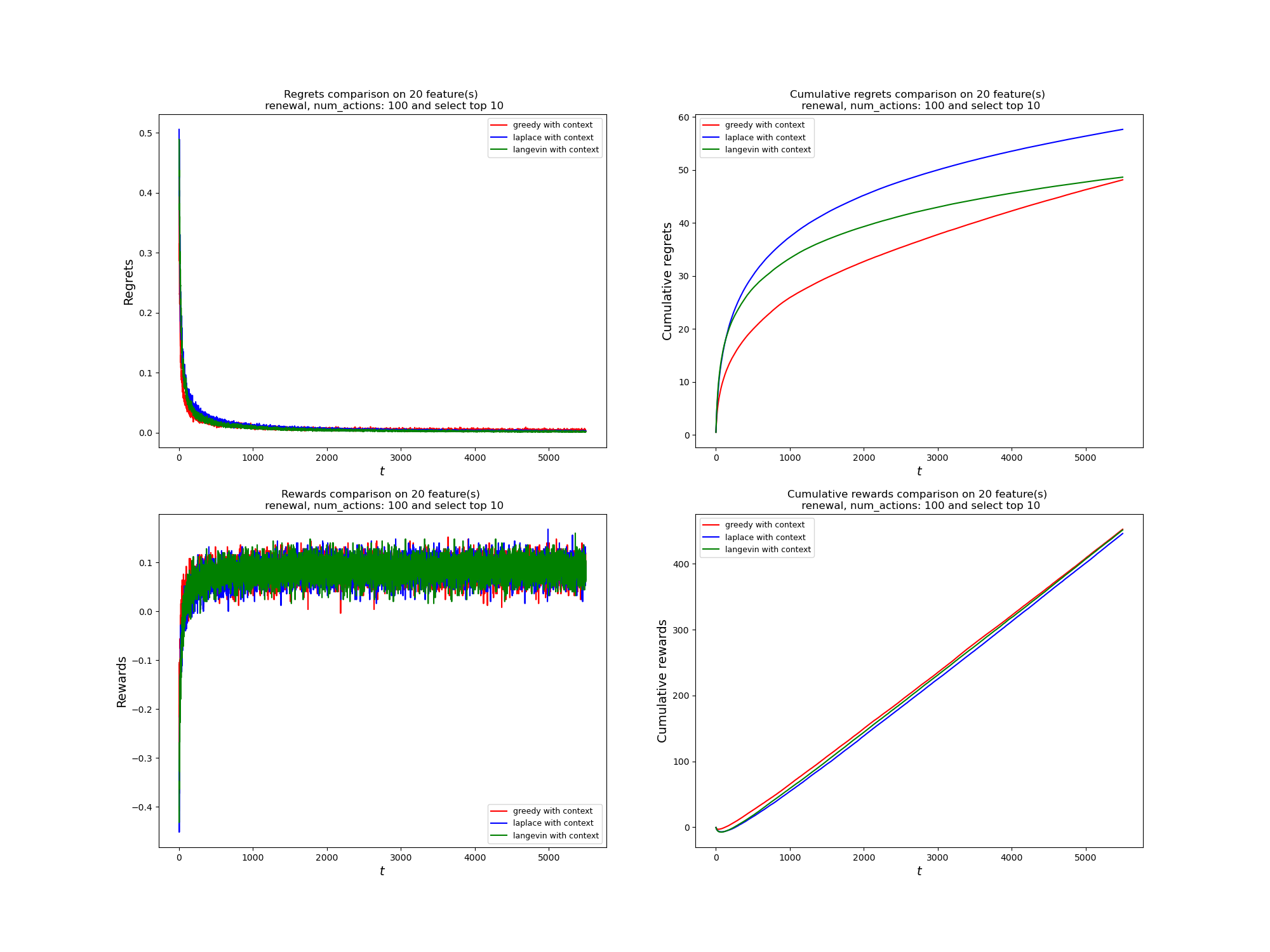
Figure 5: Performance comparison in 20-feature selecting top 10 with renewal setting

To examine even more complex environment, we focus on the last set of hyperparameter in renewal setting which sets the number of features to 20 and allows the agent to select 10 arms to play and observe the rewards. According to Figure 5, it can clearly be seen from the plot of cumulative regrets that it imitates the behaviors of the previous graphs; however, both variants of Thompson sampling take longer before its cumulative regret starts to plateau out. From this plot, Langevin MCMC has much lower cumulative regret at the end of our simulation and almost intersects with a line that represents greedy algorithm.

4 Conclusion

Although many referencing works [Bastani et al., 2020, Visantavarakul and Kiatsupaibul, 2022] have exhibited that greedy algorithms can be optimal in an envrionment with natural exploration, we raised the question of whether this would always be true. In the contextual logistic bandit, if the context features are unit vectors, exploration-based algorithms could be better than exploration-free algorithms with enough timesteps depending on the complexity of said environment.

The component of randomness in observed features has bestowed the agent with a chance to never explore but still enjoy the benefits of both worlds without the common tradeoff of exploitation-exploration which is the cardinal dilemma in traditional reinforcement learning. Nevertheless, natural exploration does not help when contexts are ungeneralizable which are expressed through simply setting context features to be identity matrix. Therefore, the study of efficient exploration is still fruitful in the scenario of credit scoring and should be encouraged to do so.

Lastly, our study has revealed another overlooked perspective of natural exploration. That is, this mechanism does not mean that an agent would never have to think about exploration but carry out the exploration for an agent to a certain degree. The more complexed the environment gets, the more the need for an agent to start exploring by itself and not relying solely on this mechanism.

Thus, there should be some sort of degree of self-exploration immured in the environment, for example, traditional envrionment with static action sets does not have any degree of self-exploration, whereas credit scoring environment has a high-degree of self-exploration. Moreover, the proof of regret bounds on greedy algorithms for such environment is still open for future work.

References

- Agrawal and Goyal [2013] Shipra Agrawal and Navin Goyal. Thompson sampling for contextual bandits with linear payoffs. In Proceedings of the 30th International Conference on International Conference on Machine Learning - Volume 28, ICML’13, page III–1220–III–1228. JMLR.org, 2013.
- Agrawal and Goyal [2017] Shipra Agrawal and Navin Goyal. Near-optimal regret bounds for thompson sampling. J. ACM, 64(5), sep 2017. ISSN 0004-5411. doi: 10.1145/3088510.
- Bastani et al. [2020] Hamsa Bastani, Mohsen Bayati, and Khashayar Khosravi. Mostly exploration-free algorithms for contextual bandits. Management Science, 67:1329–1349, 2020.
- Chapelle and Li [2011] Olivier Chapelle and Lihong Li. An empirical evaluation of thompson sampling. In J. Shawe-Taylor, R. Zemel, P. Bartlett, F. Pereira, and K.Q. Weinberger, editors, Advances in Neural Information Processing Systems, volume 24. Curran Associates, Inc., 2011.
- Dastile et al. [2020] Xolani Dastile, Turgay Celik, and Moshe Potsane. Statistical and machine learning models in credit scoring: A systematic literature survey. Applied Soft Computing, 91:106263, 2020. ISSN 1568-4946. doi: https://doi.org/10.1016/j.asoc.2020.106263.
- Dumitrascu et al. [2018] Bianca Dumitrascu, Karen Feng, and Barbara E. Engelhardt. Pg-ts: Improved thompson sampling for logistic contextual bandits. In Neural Information Processing Systems, 2018.
- Russo et al. [2018] Daniel Russo, Benjamin Roy, Abbas Kazerouni, Ian Osband, and Zheng Wen. A Tutorial on Thompson Sampling. 01 2018. ISBN 9781680834710. doi: 10.1561/9781680834710.
- Sutton and Barto [2018] Richard S Sutton and Andrew G Barto. Reinforcement learning: An introduction. MIT press, 2018.
- Visantavarakul and Kiatsupaibul [2022] Kantapong Visantavarakul and Seksan Kiatsupaibul. An application of reinforcement learning to credit scoring based on the logistic bandit framework. In International Conference on Applied Statistics (ICAS 2022), pages 112–118, 3–4 Nov 2022.
- Xu et al. [2022] Pan Xu, Hongkai Zheng, Eric V Mazumdar, Kamyar Azizzadenesheli, and Animashree Anandkumar. Langevin Monte Carlo for contextual bandits. In Proceedings of the 39th International Conference on Machine Learning, volume 162 of Proceedings of Machine Learning Research, pages 24830–24850. PMLR, 17–23 Jul 2022.