Optical polarization and spectral properties of the H-poor superluminous supernovae SN 2021bnw and SN 2021fpl

Abstract

New optical photometric, spectrocopic and imaging polarimetry data are combined with publicly available data to study some of the physical properties of the two H-poor superluminous supernovae (SLSN) SN 2021bnw and SN 2021fpl. For each SLSN, the best-fit parameters obtained from the magnetar model with MOSFiT do not depart from the range of parameter obtained on other SLSNe discussed in the literature. A spectral analysis with SYN++ shows that SN 2021bnw is a W Type, Fast evolver, while SN 2021fpl is a 15bn Type, Slow evolver. The analysis of the polarimetry data obtained on SN 2021fpl at four epochs (+1.8, +20.6, +34.1 and +43.0 days, rest-frame) shows $>3\sigma$ polarization detections in the range 0.8–1 $\%$. A comparison of the spectroscopy data suggests that SN 2021fpl underwent a spectral transition a bit earlier than SN 2015bn, during which, similarly, it could have underwent a polarization transition. The analysis of the polarimetry data obtained on SN 2021bnw do not show any departure from symmetry of the photosphere at an empirical diffusion timescale of $\approx$ 2 (+81.1 days rest-frame). This result is consistent with those on the sample of W Type SLSN observed at empirical diffusion timescale $\leq$ 1 with that technique, even though it is not clear the effect of limited spectral windows varying from one object to the other. Measurements at higher empirical diffusion timescale may be needed to see any departure from symmetry as it is discussed in the literature for SN 2017egm.

1 Introduction

H-poor superluminous supernovae have been discovered about 15 years ago (see reviews by Howell, 2017; Moriya et al., 2018; Gal-Yam, 2019; Chen, 2021). While the spectral classification frequency of such transients is quite low ($\approx 1\%$) with respect to other types of supernovae (e.g. Nicholl, 2021), spectroscopic and photometric follow-ups of Hydrogen-poor superluminous supernovae (SLSN-I) by several surveys like, among others, the Palomar Transient Factory (PTF, Rau et al., 2009) and its intermediate version (iPTF), the Dark Energy Survey (DES Angus et al., 2019) and more recently the Zwicky Transient Facility (ZTF Bellm et al., 2019), provide a large amount of data allowing more and more discoveries and time evolution studies of individual objects (e.g. Kumar et al., 2020; Könyves-Tóth et al., 2020), as well as statistical analysis of relatively large samples (e.g. Quimby et al., 2018; Angus et al., 2019; Könyves-Tóth & Vinkó, 2021; Chen et al., 2022a, b). From the light curves and spectra analyses, several models have been proposed to explain the mechanisms behind the radiate total energies of $\approx$ 10⁵¹ ergs from such objects. The current best models are those of a central engine consisting of fallback accretion on a compact object (Dexter & Kasen, 2013), or the spin-down of a newly formed magnetar (Kasen & Bildsten, 2010; Woosley, 2010). More recently, Könyves-Tóth & Vinkó (2021) found that hydrogen-poor SLSNe can be divided in two distinct groups according to their pre-maximum spectra. The members of the first group show the W-shaped absorption feature well discussed in the literature, and identified as due to O II. This feature is not observed in the second group, whose spectral shape are more similar to that of SN 2015bn. Each of these groups can also be classified as Fast or Slow evolvers based on the photospheric velocities around maximum, even though this classification may be limited by the size of the sample and the lack of object having intermediate photospheric velocities.

Polarimetry follow-ups of SLSN-I, on the other hand, are quite scarce. So far, no more than ten sources have been observed with linear polarimetry (Leloudas et al., 2015; Brown et al., 2016; Inserra et al., 2016; Leloudas et al., 2017a; Cikota et al., 2018; Maund et al., 2019, 2020; Maund et al., 2021; Lee, 2019, 2020; Saito et al., 2020; Poidevin et al., 2022; Pursiainen et al., 2022), among which three have also been observed with spectropolarimetry (2015bn, 2017egm and 2018bsz by Inserra et al., 2016; Saito et al., 2020; Pursiainen et al., 2022, respectively), and two have been probed with circular polarimetry (OGLE16dmu and LSQ14mo by Cikota et al., 2018). The main difficulty encountered by such surveys comes from the Galactic contribution and possible contributions from the SLSNe hosts possibly combined with light dilution effects by the hosts (see Leloudas et al., 2022). Such problems can in principle be tackled with spectropolarimetry if specific spectral windows in the spectra can be used to isolate the host galaxy contribution to get intrinsic polarization estimates of the SLSN (see Saito et al., 2020). Alternatively, if the host galaxy is bright enough, one could measure its intrinsic level of polarization months or years after the SLSN has faded away. This would give an integrated estimate of the level of polarization of the Galaxy that could be removed afterward from polarimetry measurements of the SLSN. If such measurements are not possible or reach observation limit sensitivities, one could still rely on the low level of polarization measured on many systems before maximum light. Most of the current available measurements obtained so far with linear polarimetry show that once the Galactic interstellar polarization (ISP) contributions have been taken into account, one can expect low degrees of polarization of order fractions of a percent before maximum light. Such results suggest that the host contribution is very low and that the light of the SLSN pervading the host ISM is not significantly polarised by magnetically aligned dust grains (see e.g. discussion in Poidevin et al., 2022). From that point, any increase in the degree of polarization measured at later phases could be attributed to a loss of the symmetry of the photosphere. Such measurements have been obtained on SN 2015bn with linear polarimetry (Leloudas et al., 2017a) and were found consistent with the results obtained with spectropolarimetry (Inserra et al., 2016). The increase of polarization is observed along a uniform polarization angle direction which is interpreted as the axis of symmetry of the inner photosphere. Alternatively, a change of polarization could come from the interaction of the photosphere with a possible disk-like, clumpy circumstellar medium (CSM) with emitting regions. This has been observed on SN 2018bsz and discussed by Pursiainen et al. (2022).

In this work we present the results obtained on the second and third target from a ten hour linear polarimetry survey conducted mainly during 2021, and designed to explore the frequency of objects like SN 2015bn and SN 2017egm. Along this work we use the Planck 2018 Flat $\Lambda-$CDM cosmology model ($\Omega_{0}=0.31,H_{0}=67.7$ km$/$s) (Planck Collaboration et al., 2020)

2 H-poor SLSN sample and hosts associations

Basic information about the two SLSN-I, SN 2021bnw and SN 2021fpl, and their possible hosts is given in Table 1.

Table 1: Information about SN 2021bnw and SN 2021fpl. Photometry and coordinates of the host candidate of SN 2021bnw are from the Dark Energy Camera Legacy Survey (DECaLS). Upper magnitude limits at the position of SN 2021fpl are from Pan-STARRS1.

Object	RASN	DecSN	redshift	$\mu$	Host	RAHOST	DecHOST	g	r	z
Name	$[^{\circ}]$	$[^{\circ}]$		[mag]	candidate	$[^{\circ}]$	$[^{\circ}]$	[mag]	[mag]	[mag]
2021bnw	163.467375	+12.55805	0.098	-38.24	Brick: 1635p125, Objid: 1948	163.4678	12.5581	19.79	19.31	19.01
2021fpl	303.577583	-18.182381	0.115	-38.59	Orphan SLSN-I ?	RASN	DecSN	> 23.6	> 23.0	> 22.6

2.1 SN 2021bnw

SN 2021bnw (ZTF object ZTF21aagpymw, Pan-STARRS 1 object PS21ajy, ATLAS object ATLAS21dpf, Gaia object Gaia21caf) was discovered by Fremling (2021) on February 03, 2021 from ZTF public alerts (Bellm et al., 2019). The discovery magnitude obtained with the ZTF-cam mounted on the Palomar 1.2 meter Oschin was of 21.07 mag in the g-filter (AB system). The transient was classified the following day as a SLSN-I at a redshift z$=0.098$ by Magee et al. (2021) (see also Terwel et al., 2021) from the analysis of a spectrum obtained by the extended Public ESO Spectroscopic Survey of Transient Objects (ePESSTO; Smartt et al., 2017) collaboration. The spectrum is publicly available on the Transient Name Server (TNS).

SN 2021bnw is very likely associated with the galaxy observed in the Dark Energy Camera Legacy Survey (DECaLS) , Data Release 9 (DR9) at position $($RA, Dec$)=(163.4678^{\circ},+12.5581^{\circ}$, J2000), of apparent magnitudes g=19.79, r=19.31, z=19.01 mag, i.e. of absolute magnitudes -18.45, -18.93 and -19.23 mag, respectively, assuming it is at the same redshift as the SLSN at z=0.098. This galaxy has also been observed in the Sloan Digitized Sky Survey (SDSS) imaging Data Release 9 (DR9) as is identified as SDSS $J105352.17+123328.5$ but the photometry obtained on that source may be unreliable .

2.2 SN 2021fpl

SN 2021fpl (ZTF object ZTF21aaxwpyv, Pan-STARRS 1 object PS21evf, ATLAS object ATLAS21iao, Gaia object Gaia21ckf) was discovered by Tonry et al. (2021) on March 16, 2021 from the Asteroid Terrestrial-impact Last Alert System (ATLAS) survey. The discovery magnitude was of 18.192 mag in the ATLAS Orange-filter (AB system). The transient was classified on 26 April, 2021 as a SLSN-I at a redshift z$=0.115$ by Deckers et al. (2021a) (see also Deckers et al., 2021b) from the analysis of a spectrum obtained with the Liverpool Telescope (LT) SPectrograph for the Rapid Acquisition of Transients (SPRAT) (Steele et al., 2004; Piascik et al., 2014). This spectrum is publicly available on the Transient Name Server (TNS).

The field of view of SN 2021fpl was observed by the Panoramic Survey Telescope and Rapid Response System (PanSTARRS-1) (Chambers et al., 2016) making this SLSN looking as an orphan SN, or with no clear association. Magnitude upper limits from PanSTARSS-1 forced photometry are displayed in Table 1 for indication. Footprints from the DeCALS DR9 and SDSS DR17 surveys do not cover the field of view of SN 2021fpl.

3 Data

3.1 Photometry

The compilation of the photometry of SN 2021bnw and SN 2021fpl used in this work are listed in Tables 12,  13 and  14, and in Tables 15,  16,  17 and  18, respectively.

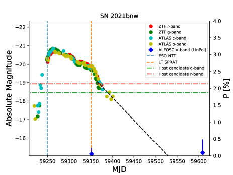
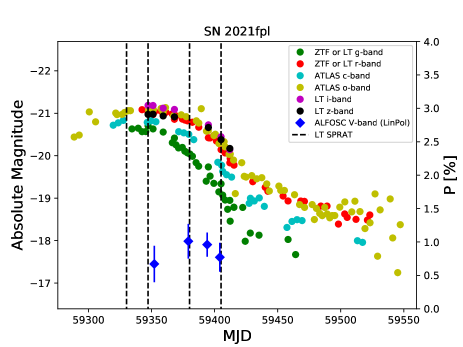
Figure 1: Top: ZTF g- and r-band, and ATLAS c- and o-band absolute light curve of SN 2021bnw. The epochs when spectroscopy was obtained are shown with dashed-lines. The absolute magnitudes of the host candidate are shown with the horizontal dashed-lines. A linear fit to the last 8 points of the light curve is shown with the dark dashed-line. The linear polarization degree, $P$, is also shown by the diamond symbol. The scale is given on the right-axis. Bottom: same as Top for SN 2021fpl with additional photometry obtained from the Liverpool Telescope in g-, r-, i- and z-bands (see Section 3.1.2 and Table 9).

3.1.1 ZTF

The ZTF g- and r-band public photometry data obtained on SN 2021bnw (ZTF21aagpymw), and on SN 2021fpl (ZTF21aaxwpyv) were all retrieved from the Lasair broker (Smith et al., 2019).

3.1.2 LT IO$:$O

Additional photometry observations were taken on SN 2021fpl in -u, -g, -r, -i and -z bands with the Liverpool Telescope IO:O instrument. The data were reduced using the AutoPhOT package (AUTOmated PHotometry Of Transients; Brennan & Fraser, 2022). The main steps of the AutoPhOT pipeline are as follows. The pipeline builds a model of the Point Spread Function (PSF) in an image from bright isolated sources in the field, or uses aperture photometry if no suitable sources are present. The instrumental magnitude is then measured from a fit of the PSF to the transient. The instrumental magnitude is calibrated onto the standard system (AB magnitudes for Sloan-like filters) from an estimate of the zero point in each image which is obtained from comparisons with catalogued standards in the field. For ugriz filters, the zero point was calculated from magnitudes of sources in the field observed by the SkyMapper Southern Observatory (Onken et al., 2019). A signal-to-noise ratio (SNR) of 5 was used to filter out bad photometry estimates. The log of the observations is displayed in Table 9.

3.1.3 ATLAS

The ATLAS forced photometry data were retrieved from the ATLAS public server (Tonry et al., 2018). The data were clipped and binned using the publicly available code plot$\_$atlas$\_$fp.py ATLAS data of SN 2021bnw were grouped in bins of one day. ATLAS data of SN 2021fpl were showing a bit more dispersion than those of 2021bnw and for that reason were binned in bins of two days.

3.1.4 Light Curves

The absolute magnitude light curves of SN 2021bnw and of SN 2021fpl are displayed in Figure 1, top and bottom, respectively. For each source, the distance modulus, $\mu=m-M$, displayed in Table 1 was used to convert the apparent magnitude (see Tables in Appendix D) to absolute magnitude. Both SLSNe peak at absolute magnitudes close to -21 mag. The public ZTF data and the public stacked and binned ATLAS data available for each of these sources are displayed in both plots. The additional photometry obtained on SN 2021fpl with the LT IO$:$O is displayed on the bottom plot in Figure 1. Spectroscopy was obtained at several epochs on each source and will be discussed in Section 3.2. The epochs of spectroscopy are marked with the vertical dashed lines in each plots. Polarimetry, was also obtained at several epochs, as will be discussed in 3.3. The fractions of polarization are shown by blue diamonds symbols (the polarization scales are given in the right-axis of each plot).

3.2 Spectroscopy

A summary of the spectroscopy obtained on SN 2021bnw and SN 2021fpl is given in Table 10.

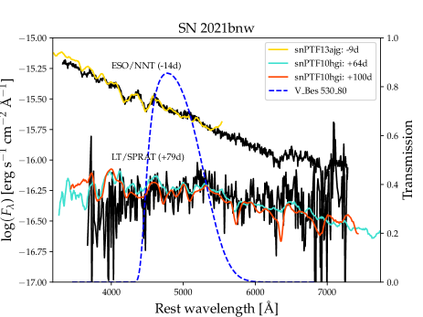
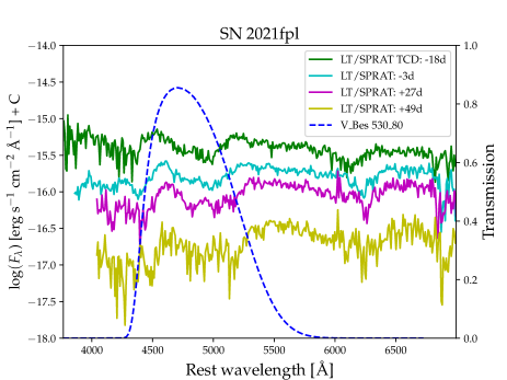
Figure 2: Spectra obtained on SN2021bnw (top) and SN2021fpl (bottom). The transmission curves of the V-band filter mounted on the ALFOSC is shown with the blue solid curve. The blue dashed curve shows the wavelength range over which polarimetry is obtained in the rest frame of each supernova.

3.2.1 SN 2021bnw

Two spectra are available on this source. We retrieved the publicly available spectrum obtained at early phase (Figure 1, top) from TNS . A second spectrum was obtained with the LT SPRAT. This spectrum was obtained about one day before polarimetry was obtained on SN 2021bnw. The two spectra obtained on SN 2021bnw are shown in Figure 2, Top. Also shown in the Figure are the transmission of the V- filter mounted on the Alhambra Faint Object Spectrograph and Camera (ALFOSC) used to get linear polarimetry data discussed in the next section. The solid line shows the filter in the observer frame while the dashed-line shows the imprint of the filter in the rest-frame of the supernova. We tested the classification and redshift of the two spectra of SN 2021bnw from a fitting template analysis with SNID, the SuperNova IDentification code, (Blondin & Tonry, 2007). To do so we used the Quimby et al. (2018) spectra database ingested in our custom SNID template library. The best match solutions displayed in Figure 2, Top, are consistent with the classification reported on TNS .

3.2.2 SN 2021fpl

Four spectra are available on that source. The first publicly available LT SPRAT spectrum used by Deckers et al. (2021a) to classify SN 2021fpl was downloaded from TNS . We obtained 3 more spectra on that source with LT SPRAT. All the spectra are displayed Figure 2, Bottom.

3.3 Polarimetry

Polarimetry on SN 2021bnw and SN 2021fpl was obtained with ALFOSC on the Nordic Optical Telescope (NOT). The observations log of the imaging polarimetry is displayed in Table 11. Linear polarimetry is made using a half wave plate in the FAPOL unit and a calcite plate mounted in the aperture wheel. The calcite plate provides the simultaneous measurement of the ordinary and the extraordinary components of two orthogonal polarized beams (see Figure 3, top and bottom). The half wave plate can be rotated in steps of 22.5^∘ from 0^∘ to $337.5^{\circ}$. As a standard, 4 angles are used ($0^{\circ},22.5^{\circ},45^{\circ}$, and $67.5^{\circ}$), which we used during our observations as referred to with the factor 4 used in the exposure time calculations displayed in Table 11. The data reduction of the polarimetry data was done using the same method and pipeline discussed in Poidevin et al. (2022). The photometry of the ordinary and extra-ordinary beams was done using aperture photometry. When taking multiple sequences of 4 HWP angles (e.g. SN 2021flp was observed 6*4*90sec) the polarization was calcutated by summing-up the fluxes from the ordinary and extra-ordinary beams to minimize uncertainty propagation. Indeed, if the polarization was calculated individually for each sequence and the Stokes parameters summed-up at the end of the process, one would have to propagate the uncertainties on $Q$ and $U$ and combine them all together. All the results and their interpretation will be discussed in Section 4.3.

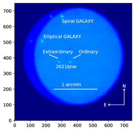
Figure 3: Top: Linear polarimetry of SN 2021bnw with ALFOSC in one of the V-band flat-field and bias corrected data frame (file ALEe170044.fits) obtained with the half-wave plate at a position angle of $0.0^{\circ}$. Each pixel embeds the number of counts obtained after an exposure of 450 seconds. Imaging polarimetry was acquired through half-wave plates positions angles at $0.0^{\circ}$, $22.5^{\circ}$, $45.0^{\circ}$ and $67.5^{\circ}$. The calcite plate splits the light from the several objects into Ordinary images and Extraordinary images separated by about $15^{\arcsec}$ from each other. Bottom: same as top for SN 2021fpl on one of the bias corrected data frame (file ALEf280162.fits) obtained after an exposure time of 90 seconds.

3.3.1 SN 2021bnw

Polarimetry was obtained on SN 2021bnw at 1 phase, about +89 days after maximum light. A measurement was obtained almost one year after maximum light (+347 days), when the SN was expected to be at least 3 to 4 magnitudes fainter than its host galaxy. This is suggested by the linear fit on the last point of the light curve of SN 2021bnw shown in Figure 1, top. The measurement at +347 days relative to peak brightness is therefore expected to reflect the polarization properties of the galaxy without any contribution from the supernovae.

3.3.2 SN 2021fpl

Polarimetry of SN 2021fpl was obtained during 4 phases. A first measurement was obtained at an epoch close to maximum light (+2 days) and 3 additional measurements were obtained during the decreasing phase (+23 days, +38 days and +48 days), before the radioactive decaying or shock-heated diffusion phase.

4 Analysis

4.1 Light Curves Modelling

There are several mechanisms which can be used to power an SLSNe light curve: nickel decay, CSM interaction, and a central magnetar. The large amount of nickel needed for SLSN light curves can only be produced in a pair instability SN, which requires an extremely massive progenitor and usually results of rise times of over 100 days (Kasen et al., 2011), which neither SN 2021bnw or SN 2021fpl show; pair instability SNe are also not expected to show significant polarization due to their quasi-spherical nature. Models using CSM interaction sometimes require unphysically high explosion energies to match both the kinetic and radiated energies inferred from observations (e.g. Chen et al., 2022b; Kangas et al., 2022) and analytic models tend to produce different results than numerical models (Moriya et al., 2018), leading to some inconsistencies in the interpretation of observations. As such, we only present light curve fits using the magnetar model.

The multi-band light curve of each SN is fitted using the "slsn" magnetar spin-down model (Nicholl et al., 2017c) in the Modular Open-Source Fitter for Transients (MOSFiT) code, which uses a Markov Chain Monte Carlo (MCMC) algorithm to perform Bayesian parameter estimation for supernova light curves (Guillochon et al., 2018). The Dynesty sampler (Speagle, 2020; Higson et al., 2019), which utilizes dynamic nested sampling is used in the process. The uncertainty presented is only the statistical uncertainty in the fits, and does not include systematic uncertainty inherent in the simplified one-zone MOSFiT model.

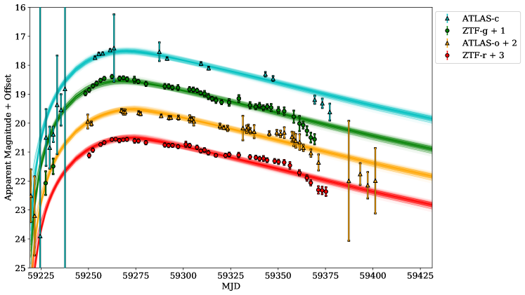
Figure 4: Multi-band light curve of SN 2021bnw inferred from the magnetar-model, with each band offset for clarity. The filled area shows the range of most likely models generated by MOSFiT. See Section 4.1 for details.

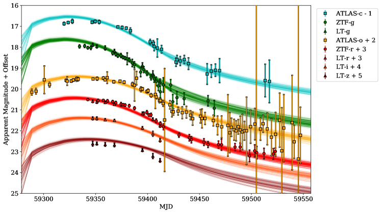
Figure 5: Multi-band light curve of SN 2021fpl inferred from the magnetar-model, with each band offset for clarity. The filled area shows the range of most likely models generated by MOSFiT. See Section 4.1 for details.

Table 2: Median and 1$\sigma$ best fit parameters for magnetar models obtained on SN 2021bnw and SN 2021fpl as discussed in Section 4.1

Parameter Symbol	Definition	Prior	Best Fit Value	Best Fit Value	Units
			SN 2021bnw	SN 2021fpl
$B_{\perp}$	Magnetar Magnetic Field Strength	[0.1,10]	$0.40^{+0.12}_{-0.11}$	$0.78^{+0.14}_{-0.17}$	1014 G
$M_{\rm NS}$	Neutron Star Mass	[1.0,2.0]	$1.58^{+0.26}_{-0.28}$	$1.71^{+0.19}_{-0.26}$	$M_{\odot}$
$P_{\rm spin}$	Magnetar Spin Period	[1,10]	$4.56^{+0.59}_{-0.64}$	$1.43^{+0.30}_{-0.24}$	ms
$\log(\kappa_{\gamma})$	Ejecta Gamma-Ray Opacity	[-4,4]	$-1.23^{+0.10}_{-0.14}$	$0.93^{1.84}_{-1.44}$	cm2 g-1
$M_{\rm ej}$	Ejecta Mass	[0.1,100]	$3.59^{+1.06}_{-0.75}$	$21.59^{+8.22}_{-4.67}$	$M_{\odot}$
$T_{\rm min}$	Photospheric Plateau Temperature	[3,10]	$9.78^{+0.14}_{-0.23}$	$5.47^{+0.54}_{-0.28}$	103 K
$v_{\rm ej}$	Ejecta Velocity	[1,20]	$7.87^{+0.50}_{-0.54}$	$6.94^{+0.28}_{-0.28}$	103 km/s

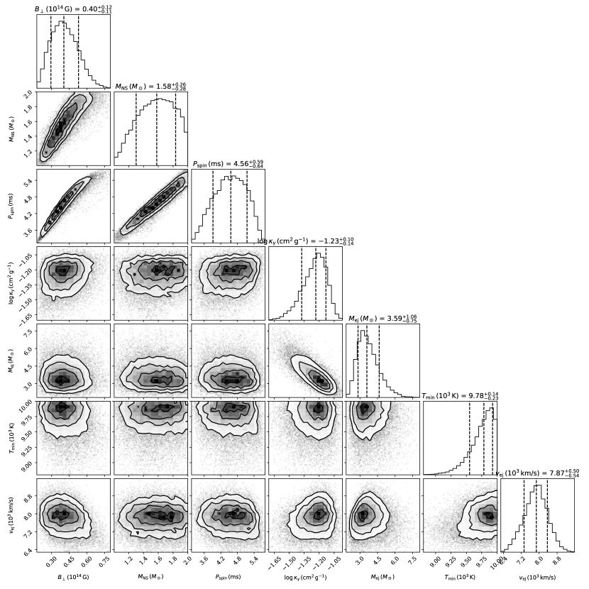
Figure 6: 1D and 2D posterior distributions of the magnetar model parameters obtained from SN 2021bnw light curve analysis with MOSFiT. Median and 1$\sigma$ values are marked and labeled - these are used as the best fit values (discussed in text).

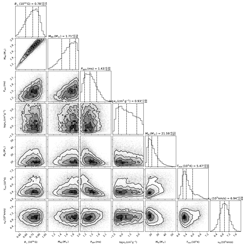
Figure 7: 1D and 2D posterior distributions of the magnetar model parameters obtained from SN 2021fpl light curve analysis with MOSFiT. Median and 1$\sigma$ values are marked and labeled - these are used as the best fit values (discussed in text).

The magnetar-model fits of SN 2021bnw and SN 2021fpl light curves are shown in Figure 4 and in Figure 5, respectively. The most physically relevant parameters are listed in Table 2, with their posteriors shown in Figure 6 for SN 2021bnw, and in Figure 7 for SN 2021fpl. The fits for both supernovae are quite good, although there are some small undulations followed by a large decrease in the luminosity of SN 2021bnw at around 100 days post-peak that is not captured by the model. The physical parameters we find for SN 2021bnw (SN 2021fpl) are $B_{\perp}\approx 4\times 10^{13}$ ($8\times 10^{13}$) G, M${}_{\rm NS}\approx$ 1.6 (1.7) $M_{\odot}$, $P_{\rm spin}\approx 4.6$ (1.4) ms, $\log(\kappa_{\gamma})\approx-1.2$ (0.9) cm² g^-1, $M_{\rm ej}\approx 3.6$ (22) $M_{\odot}$, $T_{\rm min}\approx 9800$ (5500) K, and $v_{\rm ej}\approx$ 7900 (6900) km/s; where $B_{\perp}$ is the magnetar magnetic field strength, M_NS is the neutron star mass, $P_{\rm spin}$ is the magnetar spin period, $\kappa_{\gamma}$ is the gamma-ray opacity of the ejecta (Wang et al., 2015), $M_{\rm ej}$ is the ejecta mass, $T_{\rm min}$ is the photospheric plateau temperature, and $v_{\rm ej}$ is the ejecta velocity. These best fit parameters and uncertainties are the median and 1$\sigma$ values from the one-dimensional posterior for each of the parameters. Although the parameters for these supernovae are quite different, they are both representative of the extremes of the SLSN population (Nicholl et al., 2017c), with one extreme having high spin periods and low ejecta masses (like SN 2021bnw), and the other having low spin periods and high ejecta masses (like SN 2021fpl). The total kinetic energy of the ejecta for SN 2021bnw (SN 2021fpl) is calculated to be $E_{\rm K}\approx 1.3\times 10^{51}$ ($6.2\times 10^{51}$) ergs. The mass of the progenitor stars, $M_{*}=M_{\rm NS}+M_{\rm ej}\approx 5$ (23) $M_{\odot}$, which are consistent with the $3.6-40$ $M_{\odot}$ range inferred in the mass distribution found by Blanchard et al. (2020).

We also find correlations between $B_{\perp}$, $M_{\rm NS}$, and $P_{\rm spin}$ in the 2D posterior distributions of these parameters, as in Poidevin et al. (2022), although the $P_{\rm spin}$ correlation in SN 2021fpl is not as strong as in SN 2020znr or SN 2021bnw. The cause of these correlations is still unknown.

The gamma-ray opacity is important when modelling a late-time decline in luminosity due to gamma-ray leakage. The leakage timescale is (Wang et al., 2015)

$$t_{\rm leak}\approx 80\text{ days }\left(\frac{\kappa_{\gamma}}{0.1\text{ cm${}^{2}$ g${}^{-1}$}}\right)^{1/2}\left(\frac{M_{\rm ej}}{M_{\odot}}\right)^{1/2}\left(\frac{v_{\rm ej}}{10^{4}\text{ km s${}^{-1}$}}\right)^{-1}.$$ (1)

For SN 2021bnw, $t_{\rm leak}$ $\sim$ 150 days, which is about when the light curve starts to decline. We also calculate the time when the optical depth of the ejecta $\tau_{\rm ej}=$ 1, at (Nicholl et al., 2017c)

$$t_{\rm neb}=(3\kappa M_{\rm ej}/4\pi v_{\rm ej}^{2})^{1/2},$$ (2)

where $\kappa$ is the opacity of the ejecta ($\kappa$ $\approx 0.15$ cm² g^-1 for both SNe). For SN 2021bnw, $t_{\rm neb}\sim$ 240 days, which is much later than its light curve decline. Even though the leakage time is correctly estimated, the model still cannot reproduce the observed luminosity decrease. This is likely due to a more complicated physical process than what is described by the model (Vurm & Metzger, 2021), such as CSM interaction, dust formation (Omand et al., 2019), or molecular cooling (Liljegren et al., 2022). The value of $\kappa_{\gamma}$ is not well constrained for SN 2021fpl, since there is no observed luminosity decrease that looks consistent with gamma-ray leakage.

The ejecta velocities estimated by MOSFiT are not the same as the photospheric velocity, which can be estimated from spectra, since the photospheric velocity should decrease as the photosphere recedes further into the ejecta, while the ejecta velocity should remain relatively constant post-peak, with small increases and decreases due to acceleration from the pulsar wind nebula (PWN) and collision with circumstellar material (CSM). However, the photospheric velocity at the light curve maximum can be used as a proxy for the ejecta velocity (Könyves-Tóth & Vinkó, 2021). The MOSFiT magnetar model also includes a temperature floor for the photosphere (Nicholl et al., 2017c), which is motivated by late-time observations of SLSNe (e.g. Inserra et al., 2013; Nicholl et al., 2017a) - this plateau temperature $T_{\rm min}$ can also be checked against spectral models.

4.2 Spectrum modelling

We utilized the code named SYN++ (Thomas et al., 2011) to model the available spectra of SN 2021bnw and SN 2021fpl. This code uses some local parameters that fit the lines of the individual ions and global parameters referring to the entire model spectrum. The global parameters are:

• $a_{0}$: a constant multiplier to the overall model spectrum

• $v_{\rm phot}$: the velocity at the photosphere. The uncertainty of this parameter is $\sim$ 1000 km s^-1. For detailed explanation, see Section 3.3.2. in Silverman et al. (2015).

• $T_{\rm phot}$: the temperature at the photosphere. The uncertainty of $T_{\rm phot}$ is $\sim$2000 K, discussed in Könyves-Tóth (2022)

and the local parameters are:

• $\tau$: the optical depth for the reference line of each ion

• $v_{\rm min}$: the inner velocity of the line forming region

• $v_{\rm max}$: the outer velocity of the line forming region

• $aux$: the scale height of the optical depth above the photosphere given in km s^-1. This parameter accounts for the width of the spectral features, that is in relation with the width of the line-forming region in the atmosphere. The larger the $aux$ parameter, the broader the feature.

• $T_{\rm exc}$: excitation temperature of each element/ion, assuming Local Thermodynamic Equilibrium (LTE).

The best-fit models obtained for the spectra of SN 2021bnw are shown in Figure 8, while the same in case of SN 2021fpl are plotted in Figure 9. In these figures the observed spectra are shown with black line, while green color codes the best-fit models built in SYN++. The single-ion contributions to the overall model spectra are denoted with turquoise lines shifted vertically for clarification. The local parameter values of the best-fit models can be found in Table 19 and Table 20 in the Appendix.

4.2.1 SN 2021bnw

In case of SN 2021bnw two spectra were modeled, both from the photospheric phase taken at -14 days and +77 days rest-frame phase relative to the moment of the maximum light. The date of maximum was estimated from the MOSFiT fitting as MJD 59265. As shown in the left panel of Figure 8, the pre-maximum spectrum of SN 2021bnw shows some W-shaped O II features between 4000 and 5000 Å, making this object a "Type W" SLSN-I using the classification scheme of Könyves-Tóth & Vinkó (2021). According to the best-fit SYN++ - model, the velocity of the photosphere is 20 000 km s^-1, while the photospheric temperature is 14 000 K. These are not extraordinary, but high values compared to other SLSNe. The best-fit model of the second spectrum taken at +77 days phase (see the right panel of Figure 8) contains the features of Na I, Mg II, Si II, high velocity Si II (Si II v) and Fe II. By this phase, the O II and C II lines have disappeared and the photospheric velocity swiftly decreased to 4000 km s^-1 and the temperature of the photosphere dropped to 6500 K, making SN 2021bnw a spectroscopically fast evolving event.

The estimated ejecta velocity is around 8000 km s^-1. If this is the photospheric velocity at peak, then the photospheric velocity evolution in this system was very fast at pre-peak, decreasing by a factor of $\sim$ 2.5 in two weeks, followed by a fairly slow evolution post-peak, decreasing by a factor of $\sim$ 2 in $\sim$ 2.5 months. The estimated plateau temperature is almost $\sim$ 10 000 K, which is much higher than the photospheric temperature inferred from the +77 day spectrum. This apparent discrepancy may come from model uncertainties within MOSFiT.

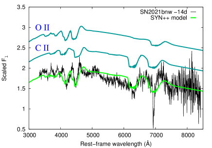
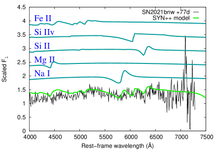
Figure 8: Top panel: Spectrum at -14 days relative to peak brightness of SN 2021bnw (black line) plotted together its best-fit model built using SYN++ (green line). Single ion contributions to the overall model spectrum (turquoise lines) are also plotted. Bottom panel: Spectrum at +77 days relative to peak brightness of SN 2021bnw together with its best-fit model. The color-coding is the same as in the left panel.

4.2.2 SN 2021fpl

We carried out the spectrum modelling of the -18 days, -3 days, +27 and +49 days phase spectrum of SN 2021fpl, as can be seen in Figure 9. We estimated the date of the maximum as MJD 59350 using the MOSFiT fitting similarly to SN 2021bnw. As the top left panel of Figure 9 shows, the earliest phase spectrum of SN 2021fpl is differing from the -14d phase spectrum of SN 2010bnw, as the former does not show the W shaped O II features between 4000 and 5000 Å, and rather can be fitted using Si II and Fe II lines. This fact makes SN 2021fpl a "Type 15bn" SLSN-I by Könyves-Tóth & Vinkó (2021). The photospheric velocity ($v_{\rm phot}=11~{}000$ km s^-1) and temperature ($T_{\rm phot}=6800$) K are also much lower compared to the similar phase spectrum of SN 2021bnw, strengthening that SN 2021fpl resembles to SN 2015bn by its pre-maximum spectrum evolution.

The -3d phase spectrum of SN 2021fpl is modeled using Si II, Fe II and Fe III lines (see the top right panel of Figure 9). By this time, the $v_{\rm phot}$ diminished to 6000 km s^-1, while the best-fit $T_{\rm phot}$ is 5700 K, a result which is broadly consistent with the MOSFiT modelling. The best-fit model of the +27d phase spectrum (see the bottom panel of Figure 9) shows similar lines and has the same photospheric velocity as the -3d phase and the photospheric temperature is similar as well (5200 K). This suggests that SN 2021fpl shows a spectroscopically slow evolution, like SN 2015bn. In Figure 9, the +49 days phase observed spectrum (red line) of SN 2021fpl is plotted together with the +27d phase spectrum (black line). It is seen that they are quite similar to each other, thus they share the best-fit SYN++ model.

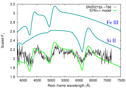
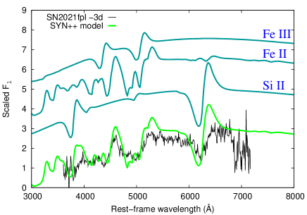
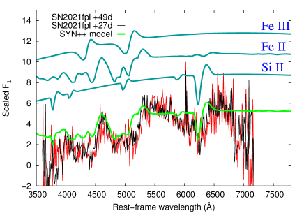
Figure 9: Top panel: modelling the -18 days phase SN 2021fpl with SYN++. Middle panel: modelling of the -3 days phase spectrum. Bottom panel: modelling of the +27 days (black) and the +49 days (red) phase spectrum. The color coding is the same as in 8.

4.3 Polarimetry Analysis

The levels of polarization obtained on polarized and unpolarized calibration stars, on SN 2021bnw, on SN 2021fpl, and on several objects of interest in their field of view, are displayed in Table 3. The steps followed to get estimates of the intrinsic polarization degree of SN 2021bnw and of SN 2021fpl (see last column in Table 3) are given in the following sections. A visual summary of all these results can be seen on the $Q-U$ plots displayed in Figure 14 for each polarimetry epoch (see Appendix F). The polarization was corrected for bias following the equation given in Wang et al. (1997):

$$P=(P_{\rm obs}-\sigma_{P}^{2}/P_{\rm obs})\times h(P_{\rm obs}-\sigma_{P}),$$ (3)

where $h$ is the Heaviside function, $P_{\rm obs}$ is the observed polarization and $\sigma_{P}$ is the 1$\sigma$ error.

Table 3: V-band polarimetry results on SN 2021bnw and its host, and on SN 2021fpl. ^(a): Stokes parameters, $\overline{Q}$ and $\overline{U}$, directly obtained from the ALFOSC data frames Extraordinary and Ordinary images without applying any further corrections. ^(b): instrumental polarization estimates. ^(c): instrumental polarization corrected. Assuming HD127769, HD251204, BD +64 106 and BD$+$32 3739 have a polarization angle of $147^{\circ}$ the zero polarization angle, $ZPA$, estimates are $83.9^{\circ}$ and $87.7^{\circ}$, respectively. ^(d): $IP$ and $ZPA$ corrected. ^(e): $IP$ and $ZPA$ corrected + Milky Way Interstellar polarization corrected with Stokes parameters obtained on star 2^(f), which is at the largest heliocentric distance, then with weighted average Stokes parameters obtained on stars STAR 1, STAR 2 and STAR 3 ^(g) (See text for details). ^(bc):bias corrected.

Date	Source	$\overline{Q}^{\rm(a)}$	$\overline{U}^{\rm(a)}$	$P[\%]^{\rm(b)}$	$P[\%]^{\rm(c)}$	$\theta[^{\circ}]^{\rm(c)}$	$P[\%]^{\rm(d)}$	$\theta[^{\circ}]^{\rm(d)}$	$P[\%]^{\rm(e)}$
2021-05-17	GD 319	0.03	-0.10	0.10 $\pm$ 0.09	…	…	…	…	…
…	HD127769	0.45	-1.41	…	1.38 $\pm$ 0.11	143.85 $\pm$ 2.37	…	…	…
…	SN 2021bnw	0.04	0.03	…	….	…	0.05 $\pm$ 0.10 (bc)	132.98 $\pm$ 20.77	…
2022-01-29	HD94851	-0.04	-0.08	0.09 $\pm$ 0.08	…	…	…	…	…
…	HD251204	-3.10	3.73	…	4.88 $\pm$ 0.18	64.38 $\pm$ 1.04	…	…	…
…	BD +64 106	5.46	1.74	…	5.80 $\pm$ 0.11	9.16 $\pm$ 0.53	…	…	…
…	SN 2021bnw Host	0.00	0.00	…	….	…	0.09 $\pm$ 0.21(bc)	-12.25 $\pm$ 23.15	…
2021-05-16	BD$+$32 3739	0.08	0.09	0.12 $\pm$ 0.09	…	…	…	…	…
…	Hiltner960	1.99	-5.51	…	5.92 $\pm$ 0.09	144.40 $\pm$ 0.44	…	…	…
…	STAR 1	-0.84	-0.06	…	….	…	0.94 $\pm$ 0.15	4.96 $\pm$ 4.57	…
…	STAR 2	-0.90	0.25	…	….	…	1.00 $\pm$ 0.22	175.91 $\pm$ 6.36	…
…	STAR 3	-0.78	-0.01	…	….	…	0.87 $\pm$ 0.40	3.86 $\pm$ 13.26	…
…	ISP	0.00	0.00	…	….	…	0.94 $\pm$ 0.12	1.63 $\pm$ 3.63	…
…	SN 2021fpl (f)	-0.16	-0.30	…	….	…	0.46 $\pm$ 0.23	29.60 $\pm$ 14.44	1.10 $\pm$ 0.25(bc)
2021-06-13	BD$+$32 3739	0.06	0.03	0.07 $\pm$ 0.06	…	…	…	…	…
…	Hiltner960	1.92	-5.30	…	5.65 $\pm$ 0.06	144.58 $\pm$ 0.31	…	…	…
…	STAR 1	-1.02	-0.28	…	….	…	1.12 $\pm$ 0.12	8.39 $\pm$ 3.17	…
…	STAR 2	-0.90	-0.14	…	….	…	0.98 $\pm$ 0.15	5.25 $\pm$ 4.35	…
…	STAR 3	-0.55	-0.16	…	….	…	0.64 $\pm$ 0.15	8.96 $\pm$ 6.84	…
…	ISP	0.00	0.00	…	….	…	0.93 $\pm$ 0.08	7.46 $\pm$ 2.50	…
…	SN 2021fpl (f)	0.19	-0.06	…	….	…	0.16 $\pm$ 0.22	71.80 $\pm$ 39.64	0.70 $\pm$ 0.23(bc)
2021-06-28	BD$+$32 3739	0.06	-0.04	0.07 $\pm$ 0.03	…	…	…	…	…
…	Hiltner960	2.06	-5.41	…	5.73 $\pm$ 0.06	145.23 $\pm$ 0.31	…	…	…
…	STAR 1	-0.78	-0.03	…	….	…	0.83 $\pm$ 0.08	179.08 $\pm$ 2.64	…
…	STAR 2	-0.58	0.05	…	….	…	0.64 $\pm$ 0.10	175.39 $\pm$ 4.31	…
…	STAR 3	-0.52	0.11	…	….	…	0.60 $\pm$ 0.09	172.16 $\pm$ 4.51	…
…	ISP	0.00	0.00	…	….	…	0.70 $\pm$ 0.05	176.21 $\pm$ 2.08	…
…	SN 2021fpl (f)	0.06	0.10	…	….	…	0.15 $\pm$ 0.13	132.89 $\pm$ 23.98	0.63 $\pm$ 0.13(bc)
2021-07-08	BD$+$32 3739	0.04	0.00	0.04 $\pm$ 0.06	…	…	…	…	…
…	Hiltner960	1.97	-5.45	…	5.79 $\pm$ 0.08	144.74 $\pm$ 0.41	…	…	…
…	STAR 1	-0.89	-0.04	…	….	…	0.93 $\pm$ 0.09	1.31 $\pm$ 2.89	…
…	STAR 2	-0.69	-0.18	…	….	…	0.75 $\pm$ 0.12	7.18 $\pm$ 4.71	…
…	STAR 3	-0.71	0.13	…	….	…	0.76 $\pm$ 0.14	175.20 $\pm$ 5.12	…
…	ISP	0.00	0.00	…	….	…	0.82 $\pm$ 0.07	1.38 $\pm$ 2.30	…
…	SN 2021fpl (f)	-0.08	-0.05	…	….	…	0.14 $\pm$ 0.17	11.70 $\pm$ 35.70	0.87 $\pm$ 0.17(bc)
4 epochs	STAR 1	…	…	…	….	…	0.95 $\pm$ 0.11	3.80 $\pm$ 3.46	…
…	STAR 2	…	…	…	….	…	0.83 $\pm$ 0.15	1.05 $\pm$ 5.35	…
…	STAR 3	…	…	…	….	…	0.70 $\pm$ 0.23	0.26 $\pm$ 9.45	…
…	ISP	…	…	…	….	…	0.85 $\pm$ 0.30	2.27 $\pm$ 10.09	…
2021-05-16	SN 2021fpl (f)	-0.16	-0.30	…	….	…	0.46 $\pm$ 0.23	29.60 $\pm$ 14.44	0.49 $\pm$ 0.38(bc)
2021-06-13	SN 2021fpl (f)	0.19	-0.06	…	….	…	0.16 $\pm$ 0.22	71.80 $\pm$ 39.64	0.84 $\pm$ 0.37(bc)
2021-06-28	SN 2021fpl (f)	0.06	0.10	…	….	…	0.15 $\pm$ 0.13	132.89 $\pm$ 23.98	0.77 $\pm$ 0.33(bc)
2021-07-08	SN 2021fpl (f)	-0.08	-0.05	…	….	…	0.14 $\pm$ 0.17	11.70 $\pm$ 35.70	0.57 $\pm$ 0.34(bc)
4 epochs	ISP (STAR 1)	…	…	…	….	…	0.95 $\pm$ 0.11	3.80 $\pm$ 3.46	…
2021-05-16	SN 2021fpl (f)	-0.16	-0.30	…	….	…	0.46 $\pm$ 0.23	29.60 $\pm$ 14.44	0.67 $\pm$ 0.26(bc)
2021-06-13	SN 2021fpl (f)	0.19	-0.06	…	….	…	0.16 $\pm$ 0.22	71.80 $\pm$ 39.64	1.01 $\pm$ 0.25(bc)
2021-06-28	SN 2021fpl (f)	0.06	0.10	…	….	…	0.15 $\pm$ 0.13	132.89 $\pm$ 23.98	0.96 $\pm$ 0.17(bc)
2021-07-08	SN 2021fpl (f)	-0.08	-0.05	…	….	…	0.14 $\pm$ 0.17	11.70 $\pm$ 35.70	0.77 $\pm$ 0.20(bc)

4.3.1 SN 2021bnw

The degree of polarization obtained after bias correction along the line-of-sight of SN 2021bnw about 3 months after maximum light (+89 days), is $p=0.05\pm 0.10\%$. This measurement, displayed in column 8 in Table 3, was obtained after instrumental polarization ($IP$), and zero polarization angle ($ZPA$) corrections only, without applying any correction to remove the polarization component foreground to the SN. Getting estimates of the Galactic polarization contribution is difficult for that source since there is no star available in the field of view covered by ALFOSC (see Figure 3, top). An alternative is to look to starlight polarization of Galactic stars compiled in the catalog provided by (Heiles, 2000). A few stars have been observed at distances about 6^∘ from the position of SN 2021bnw. Relevant data retrieved from the catalog are given in Table 5. All measurements show very low levels of polarization, with $p\leq 0.2\%$. The most relevant measurement is $p=0.166\pm 0.025\%$ from HD 91316 (see bold line) which heliocentric distance of 791.5 parsecs is the highest. If this measurement is representative of the level of polarization along the LOS of SN 2021bnw, this means that one could expect that the overall level of polarisarion of SN 2021bnw and its host is consistent with a null-polarization degree.

Since a contribution to the degree of polarization foreground to SN 2021bnw could also come from its host galaxy, we observed SN 2021bnw and its host a second time about one year after maximum light (+347 days), when the SN was more than 4 magnitudes fainter than its host (see Figure 1, top). After bias corection, the $IP$ and $ZPA$ corrected measured degree of polarization, given in column 8 in Table 3, is $p=0.09\pm 0.21\%$. This measurement is consistent with the first epoch measurement, and at the same level than the Galactic interstellar polarization estimated from the Heiles (2000) catalog in the vicinity of the system. Since the flux from the SN was negligible at this epoch, this means that the intrinsic degree of polarization of SN 2021bnw host galaxy is negligible and can be considered consistent with $0\%$ at both epochs. This result suggests that an intrinsic null-polarization degree was measured on SN 2021bnw during the first epoch measurement (+89 days). Assuming the galaxy is fully unpolarized, we also estimate that the total flux of the galaxy would dilute the polarization level measured on SN 2021bnw during the first polarimetry epoch at the level of 30$\%$ in the V-band. This means that the intrinsic polarization level of SN 2021bnw would be 1.3 higher than its estimated value, but still consistent with a null-polarization measurement.

4.3.2 SN 2021fpl

The degree of polarization obtained on SN 2021fpl at the 4 epochs are displayed in bold in the last column of Table 3. The first bias corrected 4 epochs estimates ($P=1.10\pm 0.25\%$, $P=0.70\pm 0.23\%$, $P=0.63\pm 0.13\%$ and $P=0.87\pm 0.17\%$) have been obtained following one of the methods used to derive the intrinsic level of polarization on SN 2020znr in Poidevin et al. (2022) (in the following we call it METHOD 1). At each epoch the $Q$ and $U$ Stokes parameters measured on field stars, STAR 1, STAR 2, STAR 3, were $IP$ and $ZPA$ corrected using the unpolarized and polarized stars measurements. These measurements obtained on the 3 field stars were then weighted averaged to get a final estimate of the interstellar polarization (ISP) from the Milky Way.

A look to columns 8 and 9 in Table 3 shows that, for each of the field star, the estimates obtained at the 4 epochs are almost all consistent with each other. The coordinates of these stars are displayed in Table 4. Using TOPCAT (Taylor, 2005), we cross-matched the stars coordinates with the GAIA Early Data Release 3 (EDR3) catalog in order to obtain estimates of the distances to each star. The median of the geometric distance posterior, $rgeo$, and the median of the photogeometric posterior, $rpgeo$, extracted from the catalog are displayed in column 4 and 5, respectively, in Table 4. The distance estimate to STAR 2 is of order 800 pc, while the one to STAR 3 is of about 3600 pc, and the one to STAR 1 is of order 5300 pc or higher. This seems to corroborate with the high level of polarization of order $P=0.95\pm 0.11\%$ observed on STAR 1 when the 4 epochs measurements are weighted averaged, while similar averaged measurements obtained on STAR 2 and STAR 3, are of $P=0.83\pm 0.15\%$, and of $P=0.70\pm 0.23\%$, respectively. These values are displayed in columns 8 and 9 in Table 3, under field Date $=4$ epochs. Since these 3 estimates are almost consistent with each other within their uncertainties, they were weighted averaged to get a first estimate of the global 4 epochs ISP contribution, $P(\rm{ISP})=0.85\pm 0.31\%$), and $\theta_{\rm{ISP}}=2.27\pm 10.09^{\circ}$ (METHOD 2). The relatively large uncertainty on $P$ ($\sigma_{P}=0.31\%$) coming from this combination propagates on the intrinsic estimates of $P$ obtained on SN 2021fpl at each epoch ($P=0.49\pm 0.38\%$, $P=0.84\pm 0.37\%$, $P=0.77\pm 0.33\%$ and $P=0.57\pm 0.34\%$), and leads to less accurate measurements than with METHOD 1.

Finally, since STAR 1 is the field star at the higher distance from the sun, we consider the 4 epochs weighted measurements obtained on that star, as another good proxy of the averaged ISP obtained at the 4 epochs (METHOD 3). The bias corected intrinsic level of polarization of SN 2021fpl obtained with that method are given in the last columns of the 4 last rows in Table 3. Similarly to the results obtained with METHOD 1, these estimates show $>3\sigma$ measurements, leading to the possibility that the photosphere of SN 2021fpl, observed close to and after maximum light, was not symmetrical. A result that was also observed on SN 2015bn, and on SN 2017egm.

Table 4: Gaia EDR3 distances to the field stars, STAR 1, STAR 2 and STAR 3, displayed in Figure 3. Parameter, $rgeo$, is the geometric distance, while parameter, $rpgeo$, is the photogeometric distance (see Bailer-Jones et al., 2021, for details)

Star name	RA (J2000)	Dec (J2000)	$rgeo$	$rpgeo$
	$[^{\circ}]$	$[^{\circ}]$	[pc]	[pc]
STAR 1	303.5720	-18.1781	6643.95166	5319.87744
STAR 2	303.5723	-18.1644	816.467285	776.057312
STAR 3	303.5768	-18.1864	3749.81885	3465.27148

Table 5: Starlight polarization from the Heiles (2000) agglomeration file catalog in the vicinity of SN2021bnw.

Star name	RA (J2000)	Dec (J2000)	GLON	GLAT	$P$	$\sigma_{P}$	$\theta$	$\sigma_{\theta}$	V	Heliocentric	Distance to
										Distance	SN2021bnw
	$[^{\circ}]$	$[^{\circ}]$	$[^{\circ}]$	$[^{\circ}]$	[%]	$[\%]$	$[^{\circ}]$	$[^{\circ}]$	[mag]	[pc]	$[^{\circ}]$
97179.0	167.844135	8.2670	246.8084	59.7332	0.090	0.069	53.8	21.0	9.0	436.5	6.04
91636.0	158.759130	8.6504	236.2949	52.8599	0.080	0.120	73.0	36.9	5.6	65.0	5.99
91316.0	158.202810	9.3065	234.8871	52.7675	0.166	0.025	98.1	4.3	3.8	791.5	6.09
97907.0	168.966240	13.3075	239.9347	63.7440	0.050	0.120	50.0	50.2	5.3	87.1	5.55
97633.0	168.560175	15.4297	235.3722	64.5853	0.010	0.120	93.0	80.5	3.3	25.0	5.80

5 Discussion

Table 6: Possible categorization of some SLSNe that have been probed with linear polarimetry. ^(a): Könyves-Tóth & Vinkó (2021). ^(b): This Work. ^(c): Leloudas et al. (2017b). ^(d): Nicholl et al. (2017c). ^(e): Inserra et al. (2016); Leloudas et al. (2017a). ^(f): Nicholl et al. (2017b). ^(g): Saito et al. (2020). ^(h): Lin et al. (2020) ⁽ⁱ⁾: Lee (2019). ^(j): Pursiainen et al. (2022). ^(k): Anderson et al. (2018) ^(l): Poidevin et al. (2022). ^(m): Lee (2020).

SLSN	W / 15bn(a)	Fast / Slow	$P$ (b)
	Type	evolving event	[%]
LSQ14mo	W(a)	Slow (a)	null(c)
2015bn	15bn(a)	Slow(a,d)	increase with time(e)
2017egm	W(f)	Fast(f)	increase with time(g)
2018bsz	W(j)	Slow(a,k)	change with time(j)
2020znr	W(l)	Slow(l)	null(l)
2020ank(b)	W	Fast(b)	null(m)
2021bnw	W(b)	Fast(b)	null(b)
2021fpl	15bn(b)	Slow(b)	non-zero (b)

From the previous analysis, SN 2021bnw can be classified as a fast evolver, of spectral type W, showing no evidence of intrinsic polarization over time (-14 and +77 days in the observer frame). On the other hand, SN 2021fpl is a slow evolver, of spectral type 15bn, showing hints of intrinsic polarization after maximum light ($\approx$ +23, +38 and +48 days in the observer frame). A summary of this information and similar information compiled on other type I SLSN observed with polarimetry is given in Table 6. The sample is obviously quite low for one to derive any strong conclusion but it is interesting to note that, while polarimetry is not available before maximum light on SN 2021fpl, it is showing an intrinsic level of polarization after maximum light, as does, SN 2015bn which is also classified as a slow evolver. On the other hand, since no polarimetry was obtained earlier before maximum light, a contribution from SN 2021fpl’s host galaxy can not be discarded at this stage.

To better understand SLSN-I polarization properties, in the following sections we first make a summary of the variation of the intrinsic (or at least ISP corrected) linear polarization of SLSNe as a function of their empirical diffusion timescale estimates. We then have a look at the several spectral features observed with linear polarimetry on this sample of objects. Indeed a similar filter will capture different absorption features as a function of the redshifts and phases of the transients. Such a study may help to better understand the polarization sample currently available. Then, we explore the MOSFiT space parameters to search for any correlation between SLSN-I polarization properties and the parameters inferred from the modelling of the light curves.

5.1 SLSNe light curves polarimetry sampling

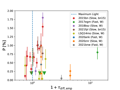
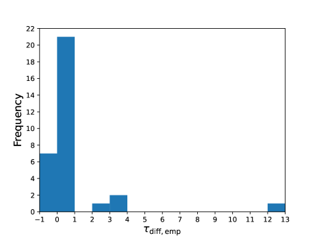
Figure 10: Top: Distribution of the degree of polarization as a function of the diffusion time scale from the sample of SLSN-I for which intrinsic polarization measurements are available. Bottom: histogram of the diffusion time scales when polarimetry was obtained.

ISP corrected or intrinsic polarization measurements have been obtained on SN 2015bn (Inserra et al., 2016; Leloudas et al., 2017a), SN 2017egm (Saito et al., 2020), SN 2018bsz (Pursiainen et al., 2022), SN 2021fpl (this work), SN LSQ14mo (see Leloudas et al., 2015, 2017b, with the second reference giving revised ISP corrected polarimetry of the data presented in the first reference.), SN 2020ank (Lee, 2020), SN 2020znr (Poidevin et al., 2022) and SN 2021bnw (this work). The polarimetry of SN 2017egm is similar to linear polarimetry obtained from spectropolarimetry after some integration in the wavelength range $\approx$ 4600–9400  Å, rest frame (see Saito et al., 2020). Linear polarimetry was also conducted by Maund et al. (2019) on that source but the measurements were lacking sensitivy therefore they are not included in this analysis. Similarily, the results obtained on SN 2018bsz are from spectropolarimetry after some integration in the wavelength range $\approx$ 3200–9100  Å, rest frame. Spectropolarimetry is also available on SN 2015bn (see Inserra et al., 2016). The data obtained at two epochs integrated over the ALFOSC V-band filter give results consistent with those obtained with linear polarimetry by Leloudas et al. (2017a), and are included in this analysis. All these spectropolarimetry data are considered and discussed in more details in Section 5.2.

Figure 10, top, shows the distribution of the polarimetry obtained on SN 2015bn, SN 2017egm, SN 2018bsz, SN 2021fpl, SN LSQ14mo, SN 2020ank, SN 2020znr and SN 2021bnw as a function of $\tau_{\rm diff,emp}+1$ (in log scale), where $\tau_{\rm diff,emp}$ is the empirical diffusion time scale. The empirical diffusion timescales were obtained by normalizing the SLSNe phases when polarimetry was measured by the rising timescale estimates retrieved from light curve analysis (see Table 7). Maximum light is shown by the vertical dashed-line in the plot. The data spread in the empirical diffusion time scale range -0.3–12.2. This is illustrated in the histogram displayed in Figure 10, bottom. Seven intrinsic polarization measurements are available before maximum light ($\tau_{\rm diff,emp}<0$). A few of them obtained on SN 2015bn are more than 3$\sigma$ detections but all of them are showing $P<0.75\%$. Departure from this limit are seen after maximum light and at empirical diffusion time scales between 0 and 1 on the transients SN 2015bn (Slow evolver, bn15 type), SN 2018bsz (Slow evolver, W type) and SN 2021fpl (Slow evolver, 15bn type), while the remaining sources (all W type) are all showing low level of polarization ($P<0.75\%$). Above $\tau_{\rm diff,emp}>1$, in the empirical diffusion time scale range $2<\tau_{\rm diff,emp}<4$, the measurements are very scarce with null-polarization detections on SN 2021bnw (Fast evolver, W type) and on SN 2020znr (Slow evolver, W type). Then another high polarization detection is available on SN 2017egm (Fast evolver, W type) at a high empirical diffusion time scale, $\tau_{\rm diff,emp}\approx 12.2$.

With a total of 32 measurements, empirical diffusion time scales are mainly sampled by polarimetry in the range, $-1<\tau_{\rm diff,emp}<1$ (28 measurements). In that domain, independently of the spectral type, only some of the slow evolvers are showing an increase of polarization and one has to probe empirical diffusion time scales $\tau_{\rm diff,emp}>3$ to detect an increase of polarization on a fast evolver (SN 2017egm). Obviously, higher polarimetry cadence samples on a larger sample of SLSN-I and on the wide range of empirical diffusion time scales discussed here ($-1<\tau_{\rm diff,emp}$ < 13) may lead to different conclusions. If such a sample was available, its interpretation could also be subject to the limit of the spectral ranges probed by linear polarimetry, when this technique is applied. For a given pass-band the spectral domain probed in the rest-frame of the SLSN will vary with the redshift and may lead to higher or lower probability to detect polarization variations. We discuss these aspects in the following section.

Table 7: Magnetar model parameters from MOSFiT for some SLSNe that have been probed with linear polarimetry. The first three have shown an increase or change in polarization over time or a non negligible level of polarization, while the rest have shown only null detections. . ^(a): If not mentioned otherwise the rise time is the estimated explosion date to g- or V-band peak, and has an uncertainty of around 10%. ^(b): Rise time estimates from Könyves-Tóth & Vinkó (2021). ^(c): Parameters will likely be estimated in Roy et al. (in prep). ^(d): Fit with MINIM (Chatzopoulos et al., 2013).

SN Name	$P_{\rm spin}$ (ms)	$B_{\perp}$ (1014 G)	$M_{\rm ej}$ ($M_{\odot}$)	$v_{\rm ej}$ (103 km/s)	$M_{\rm NS}$ ($M_{\odot}$)	Rise Time(a) (days)	Source
SN 2015bn	${2.16}_{-0.17}^{+0.29}$	${0.31}_{-0.05}^{+0.07}$	${11.73}_{-1.34}^{+0.83}$	${5.46}_{-0.14}^{+0.16}$	${1.78}_{-0.23}^{+0.28}$	90.88(b)	Nicholl et al. (2017c)
SN 2017egm	${4.38}_{-0.67}^{+0.44}$	${0.79}_{-0.22}^{+0.20}$	${3.72}_{-0.90}^{+1.65}$	${6.35}_{-0.22}^{+0.22}$	${1.67}_{-0.33}^{+0.22}$	16	Nicholl et al. (2017b)
SN 2018bsz(c)						76.17(b)	Anderson et al. (2018)
SN 2021fpl	${1.43}_{-0.24}^{+0.30}$	${0.78}_{-0.17}^{+0.14}$	${21.59}_{-4.67}^{+8.22}$	${6.94}_{-0.28}^{+0.28}$	${1.71}_{-0.26}^{+0.19}$	96	This Work
SN LSQ14mo	${4.97}_{-0.71}^{+0.65}$	${1.01}_{-0.30}^{+0.27}$	${2.10}_{-0.36}^{+0.42}$	${10.74}_{-0.41}^{+0.52}$	${1.85}_{-0.27}^{+0.22}$	34.22(b)	Nicholl et al. (2017c)
SN 2020ank(d)	${2.23}\pm 0.51$	${2.09}\pm 0.07$	$3.58\pm 0.04$	$12.27\pm 0.91$	N/A	36	Kumar et al. (2021)
SN 2020znr	${2.80}_{-0.39}^{+0.26}$	${0.52}_{-0.13}^{+0.10}$	${21.37}_{-1.43}^{+1.53}$	${5.56}_{-0.13}^{+0.13}$	${1.68}_{-0.31}^{+0.21}$	90	Poidevin et al. (2022)
SN 2021bnw	${4.56}_{-0.64}^{+0.59}$	${0.40}_{-0.11}^{+0.12}$	${3.59}_{-0.75}^{+1.06}$	${7.87}_{-0.54}^{+0.50}$	${1.58}_{-0.28}^{+0.26}$	41	This Work

Table 8: Polarimetry summary table. ^(a): as from Inserra et al. (2016) after integration of the VLT spectropolarimetry data in the ALFOSC V-band filter. ^(b):e.g. Könyves-Tóth & Vinkó (2021), ^(c): Nicholl et al. (2013), ^(d): Chen et al. (2017), ^(e): This work.

SN	Redshift	MJD (max)	MJD (pol)	pol. phase	$\tau_{\rm diff,emp}$	$P$	$\sigma_{P}$	$\lambda_{\rm min}$	$\lambda_{\rm max}$	Spectral
		[days]	[days]	[days]		$[\%]$	$[\%]$	[Å]	[Å]	Features
SN 2021fpl	0.115	59265.0	59267.0	1.8	0.02	0.67	0.26	4292.38	5782.53	Fe III, Fe II, Si II $\nu$ (e)
…	…	…	59288.0	20.6	0.24	1.01	0.25	…	…
…	…	…	59303.0	34.1	0.39	0.96	0.17	…	…
…	…	…	59313.0	43.0	0.50	0.77	0.2	…	…
SN 2015bn	0.1136	57102.0	57080.1	-19.6	-0.22	0.42	0.43	4297.77	5789.80	Fe III, Fe II(b)
…	…	…	57083.0	-17.0	-0.19	0.69	0.27	…	…	…
…	…	…	57093.0	-8.1	-0.09	0.67	0.14	…	…	…
…	…	…	57097.1	-4.4	-0.05	0.32	0.14	…	…	…
…	…	…	57108.0	5.4	0.06	0.66	0.14	…	…	…
…	…	…	57121.1	17.1	0.19	0.5	0.14	…	…	…
…	…	…	57124.1	19.8	0.22	1.0	0.14	…	…	…
…	…	…	57142.9	36.8	0.40	1.0	0.35	…	…	…
…	…	…	57153.0	45.8	0.50	1.54	0.28	…	…	Fe II, Si II, Si II$\nu$ (b)
…	…	…	57076.2	-23.7(a)	-0.25	0.12	0.07	…	…	Fe III, Fe II (b)
…	…	…	57133.0	27.5(a)	0.31	0.91	0.07	…	…	…
SN 2017egm	0.030721	57925.8	57925.2	-0.6	-0.04	0.2	…	4559.91	8828.77	OII(b)
…	…	…	57931.2	5.2	0.34	0.2	…	…	…	…
…	…	…	57935.2	9.1	0.60	0.2	…	…	…	…
…	…	…	58116.5	185.0	12.18	0.8	0.2	…	…	Fe II, Na I, [Ca II] (c)
SN 2020ank	0.22	58894.3	58909.2	12.2	0.41	0.45	0.3	3922.95	5284.85	OII(b)
SN 2021bnw	0.098	59265.0	59354.0	81.1	2.16	0.05	0.1	4358.83	5872.06	Fe II, Na I $\nu$ (e)
SN LSQ14mo	0.253	56698.9	56690.2	-6.9	-0.25	0.42	0.27	3817.06	5371.12	OII, (Si III$\nu$) (d)
…	…	…	56699.1	0.2	0.01	0.65	0.27	…	…	…
…	…	…	56709.2	8.2	0.30	0.04	0.27	…	…	Fe II, Mg II (d)
…	…	…	56715.1	12.9	0.47	0.04	0.24	…	…	…
…	…	…	56722.1	18.5	0.68	0.61	0.28	…	…	…
SN 2020znr	0.1	59233.0	59267.0	30.9	0.41	0.67	0.34	4350.91	5861.38	Fe II(c)
…	…	…	59267.0	30.9	0.41	0.19	0.32	5046.99	7747.96	Na I, Si II, [Ca II] (c)
…	…	…	59521.0	261.8	3.47	0.13	0.14	…	…	…
…	…	…	59522.0	262.7	3.48	0.26	0.2	…	…	…
SN 2018bsz	0.0267	58267.5	58278.0	10.2	0.13	0.26	0.12	3300.00	9325.00	See Pursiainen et al. (2022)
…	…	…	58307.0	38.5	0.51	1.8	0.15	…	…	…

5.2 Spectral windows observed with polarimetry

In this section we discuss and compare some of the spectral features integrated over the various filters used for linear polarimetry. The wavelength ranges covered by each filter and a summary of the polarimetry are given in Table 8. The polarization values of SN 2020ank (Lee, 2020) and SN 2020znr (Poidevin et al., 2022) were bias corrected using Equation  3. The polarization values of SN 2015bn (Inserra et al., 2016; Leloudas et al., 2017a), SN 2017egm (Saito et al., 2020), SN LSQ14mo (Leloudas et al., 2015) and SN 2018bsz (Pursiainen et al., 2022) were already bias corrected and are given as so. The spectra of SN 2015bn, SN 2017egm, SN PTF12dam and SN LSQ14mo used in this section were retrieved from the WISEReP (see Yaron & Gal-Yam, 2012) repository. When spectra on SN 2020ank, SN 2020znr are not available at phases close to the epochs when polarimetry was obtained, the spectra of SN 2017egm and SN PFT12dam are used as spectral templates for comparisons and identification of some spectral features, respectively. If not already provided by our SYN++ analysis, this information was gathered in the literature. From one study to the other, some spectral features are sometimes described with different atomic elements. The list of the most typical features are indicated in the last column of Table 8. A summary of this information is also provided on the several plots shown in Figure 11 and Figure 12.

5.2.1 15bn Type, Slow Evolver

We first focus on the 15bn Type. The polarimetry sample only contains Slow evolvers with this spectral type. SN 2021fpl (z=0.115) and SN 2015bn (z=0.1136) have very similar redshift meaning that polarimetry obtained through the ALFOSC V-band are integrating the signals over very similar wavelength ranges, making spectroscopy and polarimetry comparisons more straightforward.

Figure 11, top, shows the spectral features integrated in the linear polarimetry ALFOSC V-band filter during the observations close to and after maximum light of SN 2021fpl. Spectroscopy obtained before maximum light (-18 days) is also shown. The main absorption spectral features captured by the polarimetry filter around and after maximum light are produced by Fe II and Fe III, with contributions from Si II, as from the SYN++ analysis discussed in Section 4.2. The Fe III absorption may be less strong at phase -18 days than at higher phases and Fe II and Si II are not required to fit that spectrum, inferring a spectral transition phase occurred between -18 days and -3 days. For comparison, SN 2015bn shows a significant spectral evolution between +7 days and +20 days, with very slow spectral evolution before +7 days and after +20 days (see for example Nicholl et al., 2016). This is illustrated with the sequence of spectra displayed in Figure 11, bottom. Before a rest frame phase of +7 days SN 2015bn is very lowly polarized ($P\approx 0.5\%$) while the level of polarization is higher after +20 days (see results summarised in Table 8, results displayed in the bottom plot in Figure 11 and Leloudas et al., 2017a). The level of polarization of SN 2021fpl before maximum light is not known therefore we do not know if SN 2021fpl underwent a polarization transition phase as did SN 2015bn (Inserra et al., 2016; Leloudas et al., 2017a), during its spectral transition phase. On the other hand, despite their mild quality, the spectra, at phases -3 days, +27 days and +49 days, obtained on SN 2021fpl show similar spectral structures to those seen in the spectra obtained on SN 2015bn after $\approx$ + 20 days (see Figure 11, bottom). This gives support to the possibility that SN 2021fpl underwent a polarization transition phase earlier than SN 2015bn.

As mentioned previously, SN 2015bn was observed with spectropolarimetry by Inserra et al. (2016) at two epochs, one pre-peak at -23.7 days, and another 27.5 days after maximum in the rest-frame. The analysis of the variation of the polarization shows the presence of a dominant axis in the $Q-U$-plane with no departure from it which is interpreted as the axis of symmetry of the inner photosphere. This result was confirmed by Leloudas et al. (2017a) with the linear polarimetry data discussed before. The data obtained on SN 2021fpl also show the presence of a dominant axis over the period of about 40 days rest-frame during which polarimetry was acquired from about maximum light. The polarization angles obtained from the first to the fourth epochs given in the last 4 lines in Table 3 are $\theta=79.4^{\circ}\pm 9.9$, $\theta=90.8^{\circ}\pm 6.6$, $\theta=98.0^{\circ}\pm 4.9$ and $\theta=92.5^{\circ}\pm 7.1$, respectively.This is another interesting point suggesting that SN 2021fpl and SN 2015bn could have similar polarization properties and are part of the same class of objects. The intrinsic levels of polarization measured after SN 2015bn and SN 2021fpl underwent a spectroscopic transition are very similar to each other which also supports this hypothesis. If this is the correct this means that, similarly to SN 2015bn, the ellipticity of the photosphere of SN 2021fpl could have receded from an initially external layer with a prolate geometry of axis ratio $a/c\approx 0.9$ where $b=c$, keeping its geometry over time while the inner shell would have increased its asphericity from $\approx 0.9$ to $\approx 0.6$, as from the quantitative model proposed by Inserra et al. (2016) to interpret the increase of intrinsic linear polarization of SN 2015bn.

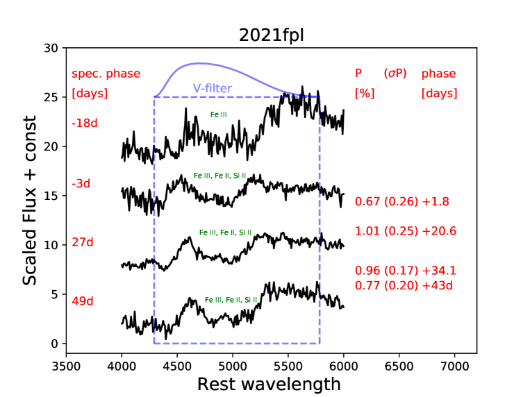
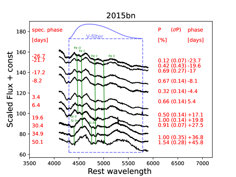
Figure 11: Spectral features observed in the rest-framed NOT ALFOSC Bessel V filter. Top: SN 2021fpl. Bottom: SN 2015bn. The phases when spectroscopy and polarimetry were obtained are indicated in red. The levels of polarization are also given. The filter band-passes are shown in blue and with the blue boxes. The main absorption spectral features integrated over the filters are shown in green.

5.2.2 W Type, Fast Evolver

SN 2017egm was observed with spectropolarimetry at 4 epochs by Saito et al. (2020). A sequence of some of the spectra publicly available on WISEReP are shown in green in Figure 12. The wavelength range over which Saito et al. (2020) made simple average of the polarization was between 4450 and 8150 Å. This is illustrated by the dashed-line green box in the Figure. Also plotted in the Figure are the publicly available spectra of SN 2020ank shown in blue, and the spectra of SN 2021bnw shown in red and discussed in this work. All together, these spectra show the spectral evolution one could roughly expect for each of these SLSN. The dashed-blue box shows the wavelength range of the V-band filter used for polarimetry on SN 2020ank by Lee (2020). One could expect the spectral feature integrated over the filter about 12 days after maximum light was mainly the well known W-shape absorption feature produced by O II and C II, as from the analysis of the -14 days rest-frame spectrum of SN 2021bnw discussed in Section 4.2. This feature is partly captured by the bandwidth used to derive the polarization level of SN 2017egm shown with the green dashed-box. All put together these results show a consistent picture suggesting that the photosphere of the W Type, Fast evolvers is still almost spherical until a few weeks after maximum light during which the W feature is still visible, i.e. the photospheres have prolate geometry of axis-ratio of order $0.9$ – $0.95$ (see Hoflich, 1991).

The filter used for polarimetry on SN 2021bnw about 80 days after maximum light is shown with the red dashed-box. The low level of polarization obtained in this filter suggests that the spectral features now produced by Fe II and Na I are associated to a photosphere still almost spherical. At later phase around +185 days SN 2017egm underwent an increase of polarization which interpretation is complex (see discussion in Saito et al., 2020). The increase in polarization could come from a loss of symmetry on the inner photosphere, but additional late epochs polarimetry would have been helpful to show if the change of polarization stands along a dominant axis as for SN 2015bn, or if it was produced by some interactions with a clumpy CSM. The Fe II and Na I already observed at earlier phase in the +77 days spectrum of SN 2021bnw are visible in the spectra of SN 2017egm close to that epoch and, for that reason, may be rejected as the cause of the change in polarization.

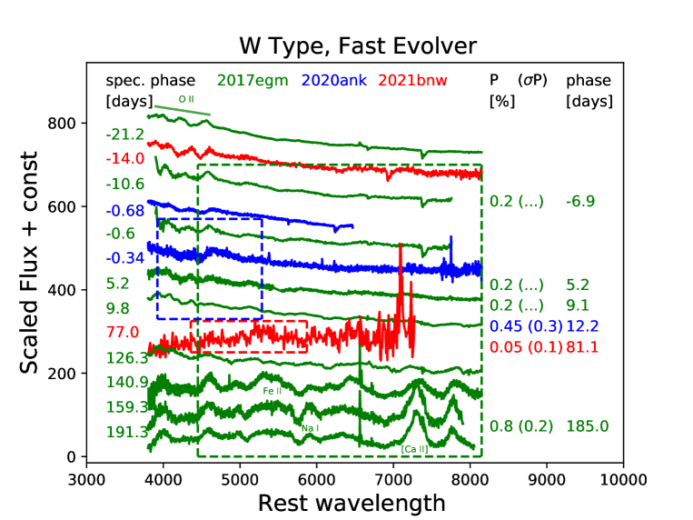
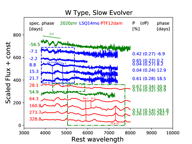
Figure 12: Top plot: Spectra of the W type, Fast Evolvers SN 2017egm (green), SN 2020ank (blue) and SN 2021bnw (red). The rest-framed NOT ALFOSC Bessel V-filters are shown with the red box for SN 2021bnw, and with the blue box for SN 2020ank. The phases when spectroscopy and polarimetry were obtained are indicated in the plot, as well as the levels of polarization. Bottom plot: same as top plot but for the Slow evolvers SN 2020znr (green), LSQ14mo (blue) and PTF12dam (red). The rest-framed V-filters wavelength ranges are shown with the blue and with the small green dashed-line boxes. The wide green dashed-line box shows the wavelength range covered by the NOT ALFOSC Bessel R-filter that was used to observe SN 2020znr.

5.2.3 W Type, Slow Evolver

SN 2018bsz has been observed with spectropolarimetry and the results are discussed by Pursiainen et al. (2022). The spectra of SN 2018bsz exhibit several features commonly seen in SLSNe but its spectral evolution looks uncommon among the W, Slow Evolver Type discussed here, with multi-component H_α profile appearing about +30 days after maximum light. The polarization results obtained by Pursiainen et al. (2022) are compiled in Table 8 and show a measurement consistent with null-polarization after maximum light (+10.2 days) while a relatively high level of polarization $P=1.80\pm 0.15$ $\%$ is found after maximum light (+38.4 days). In that case the ISP is unknown and there was a fairly significant change in polarization angle between the two epochs, for these reasons the increase of polarization is most likely explained by highly aspherical, possibly disk-like, CSM with several emitting regions. For all the reasons mentioned above, we did not add SN 2018bsz to the plot in Figure 12, bottom. On the other hand a sequence of spectra including spectra of SN 2020znr (shown in green), of LSQ14mo (shown in blue) and of SN PTF12dam (shown in red) is show in that Figure. The spectra of SN PTF12dam are assumed to be representative of the W, Slow Evolver type at epochs when polarimetry was obtained on SN 2020znr, without a spectroscopy counterpart.

In Figure 12, the blue-dashed box shows the bandwidth of the V-filter used to get polarimetry on SN LSQ14mo by Leloudas et al. (2015). The final results given by Leloudas et al. (2017b) are also given in the plot. As for Fast evolvers, the W-shape spectral feature associated to O II seems not to be polarised (-7.1 days). After that epoch the spectra show LSQ14mo underwent a spectral evolution with spectral features likely and mainly produced by Fe II and Mg II around 4300 Å (see Chen et al., 2017). The lack of high signal-to-noise ratio polarization measurements obtained after maximum light on that source suggest none of these spectral features could give insight on a loss of symmetry on the inner ejecta. The same is found at later epoch (+30.9 days) with the polarimetry of SN 2020znr in the V-filter spectral window shown with the green-dashed box. The same conclusion is corroborated by the results obtained toward the R-filter window shown with the green dashed-dotted-box in the plot. At later epoch, the V-band filter was not used and the spectral window does not include the spectral features in the wavelength range 4000–5000 Å.

5.2.4 Synthesis of the results

The results discussed in the previous section suggest than none of the several spectral groups of SLSN-I show a substantial level of polarization before maximum light. If it happens, a change of polarization property seems rather to occur after a spectral transition of the photosphere. Regarding the 15bn group, the previous analysis suggest that SN 2021fpl underwent a spectral evolution similar to SN 2015bn, and possibly a polarization evolution as well, even though, no polarimetry is available at early phase on SN 2021fpl. On the contrary, it looks like the W Type SLSNe, SN 2020ank, SN 2021bnw, SN 2020znr and SN LSQ14mo, whether they are Slow or Fast evolvers, did not undergo a polarization transition, except maybe in the case of SN 2017egm. In this spectral class, the increase of polarization observed on SN 2017egm (+185 days) lack additional polarimetry data epochs to know if the polarization would have evolved along a dominant axis. From the spectral analysis, though, it looks like the early and late spectra of SN 2017egm show H_α emission features likely coming from its host galaxy, and detected when the flux of the SLSN was not dominating the one of the galaxy. The shape of the H_α emission features is not suggesting interactions with a clumpy CSM and the increase of polarization could therefore be a probe of a loss of symmetry of the inner photosphere. From the identification or compilation of the spectral features observed by polarimetry and summarised in Table 8 it is difficult to associate any specific element to an increase of polarization. As mentioned by Saito et al. (2020) some late-phase line profiles are sensitive to the element distribution while the continuum polarization are sensitive to the distribution of the free electron which produce polarization, therefore specific studies of these two effects would be needed to disentangle them.

5.3 Light curve modelling parameter space

Based on the preceding analysis, and assuming that all SLSNe in the sample share a common progenitor that could be described by a magnetar model, we produce a comparison of the MOSFiT best fit parameters obtained with that model. Figure 13 shows the distribution of the MOSFiT best fit parameters as from Nicholl et al. (2017a) and retrieved from their work. Overplotted are the parameters obtained on SN 2015bn, SN 2017egm, SN LSQ14mo, SN 2020ank, SN 2020znr, SN 2021bnw and SN 2021fpl given in Table 7. In each plot, it is interesting to note that the MOSFiT best fit parameters of SN 2021fpl (grey star symbol) and SN 2015bn (orange disk symbol) are quite close to each other in the parameter space. The only other source, close to these two sources in each of the six plots, and on which polarimetry is available is the W Type SN 2020znr. The data at hand do not show that SN 2020znr underwent a polarization transition, may be because observations were obtained in the R-filter only (see plot in Figure 12, bottom). On the other hand, the parameters obtained for SN 2017egm share a distinct locus in the parameter space with SN LSQ14mo and SN 2021bnw, which might imply that later polarization measurements on them (which would have been too faint to be observed) would have been interesting test beds of W-type polarization properties. Finally, we point out that the kinetic energy estimate of SN 2021fpl is slightly higher than the one of SN 2015bn while SN 2015bn has twice the spin period of SN 2021fpl and a lower magnetic field. This means that the magnetar from SN 2021fpl released its energy a lot faster than SN 2015bn, which might give us hints about the possibility that the polarization transition phase of SN 2021fpl could have occurred earlier than the one of SN 2015bn. If this is true, from its position in the plot of $E_{k}$ versus spin period, SN 2020ank would also be polarized, which is not. However, the parameter inference for SN 2020ank was done using MINIM instead of MOSFiT, which may have systematic and model differences. All these facts, put together, may indicate that 15bn Type SLSNe have different polarization properties than W Type SLSNe but surely a larger polarimetry sample with higher cadence, ideally in both V- and R-filters, or with spectropolarimetry, is needed to test that hypothesis.

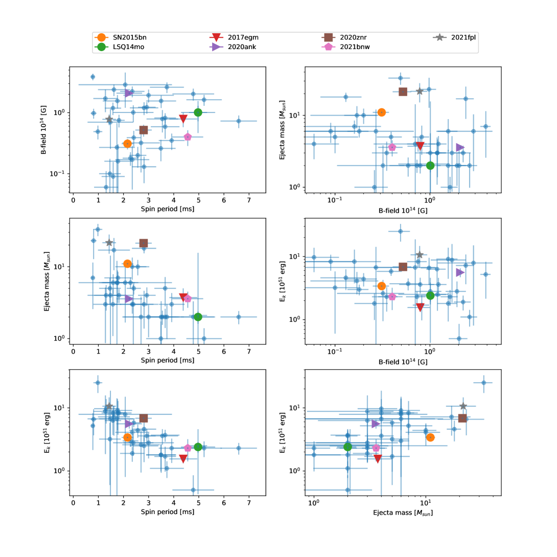
Figure 13: Distribution of the MOSFiT best fit magnetar model parameters as from Nicholl et al. (2017a). Overplotted with different coloured symbols are the parameters obtained on SN 2015bn, SN 2017egm, SN LSQ14mo, SN 2020ank, SN 2020znr, SN 2021bnw and SN 2021fpl given in Table 7, for which polarimetry data are available.

6 Conclusions

Understanding polarization properties of H-poor SLSNe to retrieve information from their inner photospheres that could help to understand the nature of their progenitor is not an easy problem to deal with. Its looks reasonable to assume that before maximum light, SLSN-I photospheres are almost spherical (This work, Inserra et al., 2016; Pursiainen et al., 2023) with low linear polarization mainly produced by Thomson scattering of light from free electrons, and this independently of the viewing angle of the inner system. According to the SYN++ analysis the photosphere temperatures of SN 2021bnw (W type) were higher compared to those of SN 2021fpl (15bn type) consistently with Könyves-Tóth (2022) when polarimetry was obtained on each of these sources. In such a case, the electron scattering opacities could have dominated over the line opacities. This could be one reason why measuring an increase of polarization after maximum light on 15bn type SLSNe-I is more likely to happen than on W type SLSNe-I, even though the 15bn type represents only about 33$\%$ of poor hydrogen SLSNe (Könyves-Tóth, 2022).

In addition to this point, it is interesting to note that none of the light curves of SN 2021bnw and SN 2021fpl show any strong bumps or undulations after maximum light, contrary to what can be seen, for example, from the the light curves of SN 2018bsz, SN 2017egm and 2017gci (see plot in Figure 5 of Pursiainen et al., 2023). After that stage, the light curves are rather smoothly decreasing. It looks therefore reasonable to assume that none of the polarization measurements obtained on these two SLSNe were possibly ’contaminated’ by polarization components that would be produced by interactions of the photospheres with the CSM, which is an important point raised by Pursiainen et al. (2023). The presence of a dominant axis in the $Q-U$ plane observed on SN 2021fpl also strengthen that hypothesis.

Finally, element mixing and clumpiness could also be additional sources of complexity on the interpretation of the polarization results (Tanaka et al., 2017). At late times, once they reach the nebular phase, the inner ejecta of SLSNe becomes visible and constraints on the nucleosynthesis and core structure from spectral analysis and modeling point out to clumped ejecta (Jerkstrand et al., 2017). SLSNe produced by stronger engines could imply more mixing and clumping in the ejecta, and possibily additional sources of asymmetry in the system, than for SLSNe produced by weaker engines (Suzuki & Maeda, 2021). From this point of view, SN 2015bn, SN 2021fpl and SN 2020znr are all located in the upper left part of the spin period versus ejecta mass diagram (see Figure 13), and can therefore be considered as strong engines. For SN 2015bn and SN 2021fpl, the increase of polarization, or high level of polarization, detected after optical maximum light could be favored by higher mixing and clumping than from weaker engines. On the other hand, as it is mentioned by Pursiainen et al. (2023), SN 2020znr (W type) was observed with polarimetry during the nebular phase but there was no detection of an increase of polarization on that source in that phase (Poidevin et al., 2022). In this case it could be that the temperature of its photosphere was still high enough to prevent the detection of the effects of a high level of mixing, or that the mass of the ejecta was so high that effects of it’s clumpy structure was still not detectable in the R-filter used for linear polarimetry, or both. It is worth noting that clumping and asymmetry can strongly affect other signals as well, such as nebular spectra (Jerkstrand et al., 2017; Dessart, 2019; Omand & Jerkstrand, 2022) and non-thermal emission (Suzuki & Maeda, 2021) in radio (Omand et al., 2018; Eftekhari et al., 2019; Law et al., 2019; Eftekhari et al., 2021; Murase et al., 2021) and x-rays (Kotera et al., 2013; Metzger et al., 2014; Murase et al., 2015; Vurm & Metzger, 2021), which may lead to correlation between polarization and these signals.

Modeling of H-poor SLSN photosphere evolution and fuller analysis of a larger observation sample might be really helpful to explore all these scenarios.

7 Summary

In this work we present new photometric, spectrocopic and imaging polarimetry data combined with publicly available data to study some of the physical properties of the two H-poor SLSN SN 2021bnw and SN 2021fpl. The spectroscopy data were obtained with LT SPRAT. The polarimetry data were obtained on the NOT with ALFOSC in the V-band filter. The photometry data were obtained on SN 2021fpl with LT IO:O. From the analysis of these data we find that:

• For each SLSN, the best-fit parameters obtained from the magnetar model with MOSFiT do not depart from the range of parameter obtained on other SLSNe discussed in the literature.

• An analysis of the spectra with SYN++ shows that SN 2021bnw is a W Type, Fast evolver, while SN 2021fpl is a 15bn Type, Slow evolver.

• An analysis of the polarimetry data shows no departure from null polarization for SN 2021bnw after maximum light (+81.1 days rest-frame), while $>3\sigma$ polarization measurements in the range 0.8–1 $\%$ are obtained for SN 2021fpl at four epochs close to and after maximum light (+1.8, +20.6, +34.1 and +43.0 days).

These results are compared with results obtained on SN 2020ank, SN 2020znr, SN 2017egm, SN 2015bn, LSQ14mo, and SN 2018bsz, a sample of SNSLe for which constrained polarization measurements are available in the literature. From these comparisons we find that:

• The majority of the polarimetry was obtained at diffuse timescale ranging between -1 and 1.

• SN 2021fpl underwent a spectroscopic transition as bit earlier than SN 2015, during which it could also have undergone a polarization transition.

• None of the photospheres of the W Type SLSNe, whether they are Slow or Fast evolvers, show a clear evidence of a departure from symmetry at empirical diffusion timescale lower than 2. The only exception being SN 2017egm which showed an increase of polarization at a empirical diffusion timescale of about 12.

• Measurements at higher empirical diffusion timescale may be needed to see any departure from symmetry of the W Type group.

Data Availability

For science reproducibility purposes the spectra presented in this work are available via WISEReP. The photometry data displayed in Table 12 to Table 14 and Table 15 to Table 18 will be available online.

Appendix A LT IO:O Observation logs

The log of the photometry obtained on SN 2021fpl with LT IO$:$O is displayed in Table 9 (see Section 3.1.2).

Table 9: Log of the photometry obtained on SN 2021fpl with the LT IO$:$O

UT Time	Exp. Time	Filter	Seeing
	[s]		[$\arcsec$]
2021-05-13 04:51:47	180	SDSS-U	1.9
2021-05-13 04:55:17	60	SDSS-G	1.6
2021-05-13 04:56:49	60	SDSS-R	1.7
2021-05-13 04:58:19	60	SDSS-I	1.3
2021-05-13 04:59:49	120	SDSS-Z	1.5
2021-05-17 03:50:52	180	SDSS-U	2.8
2021-05-17 03:54:22	60	SDSS-G	2.0
2021-05-17 03:55:55	60	SDSS-R	1.7
2021-05-17 03:57:25	60	SDSS-I	1.9
2021-05-17 03:58:55	120	SDSS-Z	1.7
2021-05-25 05:00:13	180	SDSS-U	2.3
2021-05-25 05:03:43	60	SDSS-G	2.3
2021-05-25 05:05:16	60	SDSS-R	1.8
2021-05-25 05:06:47	60	SDSS-I	1.7
2021-05-25 05:08:18	120	SDSS-Z	1.5
2021-06-03 03:10:09	180	SDSS-U	1.8
2021-06-03 03:13:38	60	SDSS-G	1.4
2021-06-03 03:15:11	60	SDSS-R	1.5
2021-06-03 03:16:42	60	SDSS-I	1.4
2021-06-03 03:18:12	120	SDSS-Z	1.4
2021-06-09 02:28:37	180	SDSS-U	7.9
2021-06-09 02:32:06	60	SDSS-G	5.4
2021-06-09 02:33:39	60	SDSS-R	…
2021-06-09 02:35:09	60	SDSS-I	5.2
2021-06-09 02:36:39	120	SDSS-Z	3.8
2021-06-15 03:50:25	180	SDSS-U	1.4
2021-06-15 03:53:54	60	SDSS-G	1.2
2021-06-15 03:55:26	60	SDSS-R	1.1
2021-06-15 03:56:57	60	SDSS-I	1.3
2021-06-15 03:58:27	120	SDSS-Z	1.2
2021-06-30 01:02:01	180	SDSS-U	1.6
2021-06-30 01:05:30	60	SDSS-G	1.4
2021-06-30 01:07:02	60	SDSS-R	1.3
2021-06-30 01:08:33	60	SDSS-I	1.2
2021-06-30 01:10:04	120	SDSS-Z	1.4
2021-07-10 02:43:23	180	SDSS-U	3.4
2021-07-10 02:46:53	60	SDSS-G	2.5
2021-07-10 02:48:24	60	SDSS-R	2.4
2021-07-10 02:49:54	60	SDSS-I	3.3
2021-07-10 02:51:25	120	SDSS-Z	2.7
2021-07-17 01:54:31	180	SDSS-U	1.8
2021-07-17 01:57:59	60	SDSS-G	1.5
2021-07-17 01:59:31	60	SDSS-R	1.5
2021-07-17 02:01:01	60	SDSS-I	1.2
2021-07-17 02:02:31	120	SDSS-Z	1.2

Appendix B Spectroscopy Observation logs

Information about the spectroscopy obtained on SN 2021bnw and 2021fpl is given in Table 10 (see Section 3.2).

Table 10: Spectra obtained on SN 2021bnw and SN 2021fpl

Source	UT Time	Telescope/Instrument	Exp. Time	Observer/s	reducer/s	Group
			[s]
SN 2021bnw	2021-02-04 06:59:55	ESO-NTT / EFOSC2-NTT	600	M. Magee, J. Terwel	S. Prentice, L. Harvey	ePESSTO+
SN 2021bnw	2021-05-16 23:39:45	LT / SPRAT	3$\times$ 300	I. Pérez-Fournon	I. Pérez-Fournon	This work
SN 2021fpl	2021-04-26 05:17:50	LT / SPRAT	?	S. Prentice	M. Deckers	TCD
SN 2021fpl	2021-05-13 04:27:30	LT / SPRAT	3$\times$ 240	I. Pérez-Fournon	I. Pérez-Fournon	This work
SN 2021fpl	2021-06-15 03:33:31	LT / SPRAT	3$\times$ 300	I. Pérez-Fournon	I. Pérez-Fournon	This work
SN 2021fpl	2021-07-10 02:23:54	LT / SPRAT	3$\times$ 350	I. Pérez-Fournon	I. Pérez-Fournon	This work

Appendix C ALFOSC polarimetry Observation logs

The observation logs of the imaging polarimetry obtained on SN 2021bnw, on its host and on SN 2021fpl are displayed in Table 11 (see Section 3.3).

Table 11: Observations log of the imaging polarimetry observations.

UT Time	Object	Exp. Time	Filter	Seeing
		[s]		[$\arcsec$]
2021-05-17 22:11:48	SN 2021bnw	$1\times(4\times 450$)	V	1.9
2021-05-17 22:53:56	HD127769	$2\times(4\times 1)$	V	1.5
2021-05-17 22:57:30	GD319	$2\times(4\times 5)$	V	1.3
2021-05-18 03:18:03	SN 2021fpl	$5\times(4\times 45)$	V	1.0
2021-05-18 04:00:19	BD+32 3739	$1\times(4\times 2)$	V	0.8
2021-05-18 04:03:33	Hiltner960	$1\times(4\times 5)$	V	0.8
2021-06-14 04:34:33	SN 2021fpl	$7\times(4\times 45)$	V	0.7
2021-06-14 05:01:40	BD+32 3739	$1\times(4\times 2)$	V	0.7
2021-06-14 05:04:25	Hiltner960	$1\times(4\times 5)$	V	0.6
2021-06-29 02:24:13	SN 2021fpl	$5\times(4\times 90)$	V	0.7
2021-06-29 02:59:49	BD+32 3739	$3\times(4\times 2)$	V	0.7
2021-06-29 03:03:41	Hiltner960	$2\times(4\times 5)$	V	0.9
2021-07-09 03:11:58	SN 2021fpl	$6\times(4\times 90)$	V	1.6
2021-07-09 03:55:12	BD+32 3739	$3\times(4\times 2)$	V	1.3
2021-07-09 03:59:23	Hiltner960	$2\times(4\times 5)$	V	1.3
2022-01-29 20:24:46	BD+64 106	$3\times(4\times 1)$	V	1.2
2022-01-30 01:36:31	HD25120	$4\times(4\times 1)$	V	0.9
2022-01-30 01:42:57	HD94851	$4\times(4\times 1)$	V	1.1
2022-01-30 03:43:06	SN 2021bnw Host	$1\times(4\times 900)$	V	0.9

Appendix D Photometry Table

The photometry from SN 2021bnw and SN 2021fpl used along this work are compiled in Table 12 to Table 14 and Table 15 to Table 18, respectively (see Section 3.1 and Section 4.1).

Table 12: ZTF and ATLAS photometry of SN 2021bnw.

MJD	Magnitude	$\sigma_{\rm Magnitude}$	band	survey
59219.640000	20.508	0.907	r	ATLAS
59221.630000	21.202	1.363	r	ATLAS
59224.540000	23.900	9.375	r	ATLAS
59227.440637	21.072	0.408	r	ZTF
59227.640000	20.496	0.978	g	ATLAS
59229.570000	20.845	0.721	g	ATLAS
59231.419965	20.492	0.266	r	ZTF
59231.500000	20.389	0.261	g	ATLAS
59233.480000	19.368	1.702	c	ATLAS
59235.540000	19.543	0.539	c	ATLAS
59237.640000	18.816	37.824	c	ATLAS
59248.414120	17.973	0.064	r	ZTF
59249.660000	17.944	0.238	r	ATLAS
59250.370023	17.857	0.064	g	ZTF
59250.377361	18.115	0.067	g	ZTF
59251.570000	18.016	0.068	g	ATLAS
59252.318773	17.934	0.058	g	ZTF
59252.379005	17.713	0.056	sdssg	ZTF
59253.450000	17.737	0.044	c	ATLAS
59254.300023	17.620	0.058	r	ZTF
59255.460000	17.605	0.037	c	ATLAS
59256.369352	17.520	0.051	sdssg	ZTF
59256.399120	17.740	0.045	g	ZTF
59257.510000	17.587	0.025	g	ATLAS
59258.341076	17.671	0.046	sdssr	ZTF
59258.366447	17.454	0.051	g	ZTF
59261.440000	17.474	0.024	r	ATLAS
59262.349213	17.565	0.046	g	ZTF
59262.410694	17.394	0.057	r	ZTF
59263.480000	17.406	1.162	g	ATLAS
59264.360023	17.552	0.043	r	ZTF
59266.332535	17.603	0.056	g	ZTF
59266.417014	17.452	0.062	sdssg	ZTF
59267.460000	17.566	0.051	r	ATLAS
59268.354398	17.577	0.038	g	ZTF
59268.410000	17.614	0.089	g	ATLAS
59268.431817	17.434	0.050	r	ZTF
59269.350000	17.618	0.087	r	ATLAS
59270.309595	17.563	0.050	g	ZTF
59270.382465	17.477	0.061	r	ZTF
59274.239607	17.500	0.104	sdssg	ZTF
59274.359919	17.611	0.066	r	ZTF
59276.256076	17.561	0.056	g	ZTF
59276.337083	17.616	0.054	g	ZTF
59276.480000	17.646	0.056	o	ATLAS
59277.470000	17.675	0.052	r	ATLAS
59280.286493	17.674	0.054	r	ZTF
59280.286493	17.674	0.054	sdssr	ZTF
59280.359826	17.644	0.070	g	ZTF
59287.380000	17.534	0.319	g	ATLAS
59288.360000	17.751	0.043	o	ATLAS
59290.255706	17.756	0.056	g	ZTF
59290.295637	17.728	0.079	sdssg	ZTF
59291.440000	17.770	0.043	g	ATLAS
59292.254606	17.774	0.052	sdssr	ZTF
59292.294757	17.728	0.072	r	ZTF
59292.430000	17.812	0.060	o	ATLAS
59293.420000	17.808	0.049	r	ATLAS
59294.253889	17.770	0.066	g	ZTF
59294.319282	17.768	0.053	r	ZTF
59297.205984	17.774	0.088	sdssg	ZTF

Table 13: ZTF and ATLAS photometry of SN 2021bnw.

MJD	Magnitude	$\sigma_{\rm Magnitude}$	band	survey
59297.256701	17.809	0.054	r	ZTF
59297.450000	17.810	0.070	o	ATLAS
59301.356435	17.733	0.091	g	ZTF
59303.278657	17.830	0.072	r	ZTF
59303.351562	17.769	0.056	g	ZTF
59303.400000	17.853	0.123	g	ATLAS
59304.430000	17.859	0.070	r	ATLAS
59305.290150	17.846	0.070	sdssg	ZTF
59305.290150	17.846	0.070	sdssg	ZTF
59305.520000	17.938	0.142	o	ATLAS
59307.247315	17.835	0.056	g	ZTF
59307.279155	17.873	0.060	r	ZTF
59309.192778	17.956	0.053	sdssg	ZTF
59309.233009	17.962	0.051	g	ZTF
59309.360000	17.943	0.048	r	ATLAS
59311.170463	17.930	0.064	r	ZTF
59311.211875	17.984	0.095	sdssg	ZTF
59313.212685	18.025	0.060	sdssr	ZTF
59313.233762	18.082	0.090	g	ZTF
59313.380000	18.104	0.049	g	ATLAS
59315.211956	18.159	0.066	r	ZTF
59317.192662	18.113	0.043	sdssr	ZTF
59317.192662	18.113	0.043	r	ZTF
59317.233762	18.213	0.086	r	ZTF
59317.233762	18.213	0.086	sdssg	ZTF
59319.350000	18.100	0.085	o	ATLAS
59320.173715	18.278	0.068	g	ZTF
59321.350000	18.154	0.048	r	ATLAS
59322.270417	18.117	0.057	r	ZTF
59323.360000	18.179	0.092	o	ATLAS
59324.171412	18.286	0.109	r	ZTF
59324.171412	18.286	0.109	g	ZTF
59324.171412	18.286	0.109	g	ZTF
59324.212095	18.084	0.060	sdssr	ZTF
59324.212095	18.084	0.060	g	ZTF
59324.212095	18.084	0.060	sdssr	ZTF
59329.232905	18.103	0.073	r	ZTF
59329.232905	18.103	0.073	sdssr	ZTF
59329.232905	18.103	0.073	g	ZTF
59329.312373	18.148	0.113	r	ZTF
59329.312373	18.148	0.113	r	ZTF
59329.312373	18.148	0.113	sdssg	ZTF
59331.420000	18.169	0.421	g	ATLAS
59333.390000	18.211	0.127	o	ATLAS
59334.340000	18.138	0.084	o	ATLAS
59335.191123	18.167	0.059	g	ZTF
59335.211921	18.384	0.108	r	ZTF
59335.340000	18.259	0.088	r	ATLAS
59337.360000	18.292	0.222	g	ATLAS
59338.192245	18.434	0.086	sdssg	ZTF
59338.237176	18.186	0.060	g	ZTF
59340.192211	18.390	0.089	r	ZTF
59340.233472	18.228	0.063	sdssr	ZTF
59342.235521	18.467	0.084	r	ZTF
59342.290637	18.220	0.083	g	ZTF
59343.300000	18.311	0.076	c	ATLAS
59344.208750	18.279	0.064	sdssr	ZTF
59344.269143	18.428	0.077	g	ZTF
59345.350000	18.353	0.076	g	ATLAS
59346.331991	18.461	0.119	sdssg	ZTF
59347.350000	18.460	0.085	c	ATLAS

Table 14: ZTF and ATLAS photometry of SN 2021bnw.

MJD	Magnitude	$\sigma_{\rm Magnitude}$	band	survey
59348.175706	18.308	0.066	g	ZTF
59349.310000	18.326	0.094	r	ATLAS
59350.177998	18.554	0.108	r	ZTF
59350.229606	18.338	0.073	sdssr	ZTF
59351.290000	18.370	0.107	g	ATLAS
59353.192778	18.356	0.084	r	ZTF
59353.221829	18.587	0.128	g	ZTF
59353.260000	18.327	0.182	r	ATLAS
59356.235822	18.461	0.112	sdssr	ZTF
59357.310000	18.471	0.170	g	ATLAS
59358.257118	18.778	0.209	g	ZTF
59358.280000	18.552	0.236	o	ATLAS
59359.310000	18.611	0.235	o	ATLAS
59361.194583	18.713	0.090	sdssr	ZTF
59361.255590	19.017	0.261	sdssg	ZTF
59361.350000	18.653	0.268	o	ATLAS
59363.214005	19.069	0.115	sdssg	ZTF
59363.310000	18.853	0.106	r	ATLAS
59365.181620	18.894	0.093	sdssr	ZTF
59365.204595	19.263	0.154	g	ZTF
59367.208229	19.062	0.091	sdssr	ZTF
59367.233565	19.498	0.169	sdssg	ZTF
59367.290000	19.034	0.125	o	ATLAS
59369.224005	19.556	0.174	g	ZTF
59369.300000	19.191	0.139	r	ATLAS
59371.225613	19.308	0.125	sdssr	ZTF
59371.310000	19.359	0.272	o	ATLAS
59373.217245	19.325	0.125	sdssr	ZTF
59373.300000	19.315	0.160	r	ATLAS
59375.226968	19.365	0.148	sdssr	ZTF
59377.260000	19.617	0.289	c	ATLAS
59387.270000	19.994	2.072	o	ATLAS
59393.260000	19.759	0.372	o	ATLAS
59397.260000	20.146	0.453	o	ATLAS
59401.250000	19.989	1.128	o	ATLAS

Table 15: ZTF and ATLAS photometry of SN 2021fpl.

MJD	Magnitude	$\sigma_{\rm Magnitude}$	band	survey
59288.630000	18.151	0.135	o	ATLAS
59292.630000	18.105	0.134	o	ATLAS
59300.620000	17.559	0.661	o	ATLAS
59305.620000	17.793	0.115	o	ATLAS
59319.620000	17.872	0.065	c	ATLAS
59321.600000	17.586	0.054	o	ATLAS
59322.610000	17.622	0.202	o	ATLAS
59323.590000	17.817	0.052	c	ATLAS
59326.590000	17.619	0.054	o	ATLAS
59327.580000	17.759	0.096	c	ATLAS
59328.610000	17.572	0.054	o	ATLAS
59331.600000	17.531	0.100	o	ATLAS
59333.270000	17.530	0.080	o	ATLAS
59334.480243	17.959	0.072	sdssg	ZTF
59339.425671	17.944	0.069	sdssg	ZTF
59342.440185	17.506	0.044	sdssr	ZTF
59342.461933	18.025	0.059	sdssg	ZTF
59345.421933	18.023	0.088	sdssg	ZTF
59346.590000	17.806	0.056	c	ATLAS
59347.205057	17.883	0.073	sdssg	LT
59347.206127	17.586	0.060	sdssr	LT
59347.207162	17.405	0.068	sdssi	LT
59347.208211	17.618	0.112	sdssz	LT
59347.540000	17.522	0.043	o	ATLAS
59349.560000	17.769	0.064	c	ATLAS
59351.162752	17.960	0.074	sdssg	LT
59351.163828	17.623	0.060	sdssr	LT
59351.164874	17.408	0.070	sdssi	LT
59351.165920	17.612	0.065	sdssz	LT
59351.480000	17.505	0.073	o	ATLAS
59352.424387	17.553	0.059	sdssr	ZTF
59353.470000	17.791	0.079	c	ATLAS
59357.461401	17.540	0.041	sdssr	ZTF
59357.540000	17.478	0.060	o	ATLAS
59359.170000	17.561	0.049	o	ATLAS
59359.210918	18.034	0.096	sdssg	LT
59359.211989	17.643	0.049	sdssr	LT
59359.213040	17.471	0.048	sdssi	LT
59359.214095	17.655	0.084	sdssz	LT
59361.110000	17.457	0.273	o	ATLAS
59361.419190	17.568	0.055	sdssr	ZTF
59366.415613	17.606	0.053	sdssr	ZTF
59366.451863	18.285	0.076	sdssg	ZTF
59367.480000	17.653	0.055	o	ATLAS
59368.134473	18.176	0.069	sdssg	LT
59368.135543	17.732	0.046	sdssr	LT
59368.136592	17.501	0.038	sdssi	LT
59368.137643	17.676	0.086	sdssz	LT
59369.376401	18.335	0.076	sdssg	ZTF
59369.441238	17.652	0.056	sdssr	ZTF
59371.397963	18.409	0.069	sdssg	ZTF
59371.490000	18.024	0.047	c	ATLAS
59373.530000	17.627	0.050	o	ATLAS
59374.398518	18.396	0.097	sdssg	ZTF
59374.438843	17.728	0.085	sdssr	ZTF
59375.540000	18.053	0.059	c	ATLAS
59376.398866	18.485	0.061	sdssg	ZTF
59376.437940	17.751	0.048	sdssr	ZTF
59377.490000	17.671	0.056	o	ATLAS
59378.396910	17.769	0.054	sdssr	ZTF
59378.419213	18.523	0.070	sdssg	ZTF

Table 16: ZTF and ATLAS photometry of SN 2021fpl.

MJD	Magnitude	$\sigma_{\rm Magnitude}$	band	survey
59379.520000	18.086	0.055	c	ATLAS
59380.405000	18.552	0.281	sdssg	ZTF
59382.357153	17.803	0.061	sdssr	ZTF
59382.414201	18.605	0.088	sdssg	ZTF
59383.480000	18.212	0.134	c	ATLAS
59385.317766	18.755	0.177	sdssg	ZTF
59385.510000	17.769	0.084	o	ATLAS
59387.357014	18.839	0.144	sdssg	ZTF
59387.421238	17.920	0.065	sdssr	ZTF
59387.460000	17.822	0.756	o	ATLAS
59389.420000	17.482	0.319	o	ATLAS
59393.335301	19.192	0.220	sdssg	ZTF
59393.560000	18.014	0.113	o	ATLAS
59395.040000	17.997	0.063	o	ATLAS
59395.045484	18.856	0.108	sdssg	LT
59395.046556	18.168	0.063	sdssr	LT
59395.047606	17.865	0.059	sdssi	LT
59395.048655	17.926	0.066	sdssz	LT
59396.378276	18.173	0.071	sdssr	ZTF
59396.419769	19.072	0.142	sdssg	ZTF
59399.378588	18.114	0.078	sdssr	ZTF
59399.398901	19.243	0.107	sdssg	ZTF
59399.460000	18.117	0.062	o	ATLAS
59400.600000	18.085	0.078	o	ATLAS
59401.419143	18.245	0.059	sdssr	ZTF
59402.520000	18.746	0.122	c	ATLAS
59403.334491	18.241	0.082	sdssr	ZTF
59403.376840	19.444	0.119	sdssg	ZTF
59403.460000	18.305	0.083	o	ATLAS
59405.115887	19.254	0.120	sdssg	LT
59405.116946	18.448	0.061	sdssr	LT
59405.117988	18.145	0.118	sdssi	LT
59405.119034	18.211	0.116	sdssz	LT
59405.560000	18.816	0.130	c	ATLAS
59406.373866	19.520	0.156	sdssg	ZTF
59406.440000	18.961	0.202	c	ATLAS
59407.540000	18.262	0.668	o	ATLAS
59408.332465	18.526	0.087	sdssr	ZTF
59408.336262	19.636	0.204	sdssg	ZTF
59408.420000	18.384	0.086	o	ATLAS
59409.440000	19.039	0.432	c	ATLAS
59410.335984	19.854	0.223	sdssg	ZTF
59411.460000	18.560	0.101	o	ATLAS
59412.081938	19.644	0.122	sdssg	LT
59412.082998	18.759	0.072	sdssr	LT
59412.084038	18.450	0.081	sdssi	LT
59412.085085	18.421	0.083	sdssz	LT
59412.335116	20.134	0.282	sdssg	ZTF
59412.357037	18.656	0.076	sdssr	ZTF
59412.430000	18.553	0.087	o	ATLAS
59413.480000	19.096	0.180	c	ATLAS
59415.020000	18.694	0.134	o	ATLAS
59415.289873	19.807	0.343	sdssg	ZTF
59415.289873	19.807	0.343	sdssg	ZTF
59415.358368	18.812	0.137	sdssr	ZTF
59415.358368	18.812	0.137	sdssr	ZTF
59416.410000	19.484	2.462	o	ATLAS
59421.510000	18.756	0.197	o	ATLAS
59422.277384	19.811	0.261	sdssg	ZTF
59423.490000	19.076	0.254	o	ATLAS
59424.272523	20.608	0.340	sdssg	ZTF

Table 17: ZTF and ATLAS photometry of SN 2021fpl.

MJD	Magnitude	$\sigma_{\rm Magnitude}$	band	survey
59424.900000	19.094	0.156	o	ATLAS
59427.390000	19.714	0.198	c	ATLAS
59428.294340	20.415	0.297	sdssg	ZTF
59428.390000	19.594	0.201	c	ATLAS
59429.450000	19.061	0.181	o	ATLAS
59430.251817	19.204	0.105	sdssr	ZTF
59431.450000	19.658	0.214	c	ATLAS
59433.450000	19.136	0.285	o	ATLAS
59435.214213	20.464	0.277	sdssg	ZTF
59435.420000	19.586	0.192	c	ATLAS
59437.430000	19.109	0.278	o	ATLAS
59439.420000	19.785	0.276	c	ATLAS
59440.230671	19.335	0.148	sdssr	ZTF
59440.230671	19.335	0.148	sdssr	ZTF
59441.350000	19.257	0.213	o	ATLAS
59442.232188	19.429	0.148	sdssr	ZTF
59443.410000	19.423	0.309	o	ATLAS
59450.960000	19.307	0.321	o	ATLAS
59452.430000	19.410	0.452	o	ATLAS
59454.292998	19.541	0.161	sdssr	ZTF
59455.360000	19.410	0.283	o	ATLAS
59457.380000	20.282	0.491	c	ATLAS
59458.230266	19.658	0.141	sdssr	ZTF
59458.251817	20.566	0.245	sdssg	ZTF
59461.350000	20.141	0.298	c	ATLAS
59463.360000	19.510	0.258	o	ATLAS
59464.231701	20.922	0.369	sdssg	ZTF
59465.350000	20.098	0.292	c	ATLAS
59467.360000	19.743	0.450	o	ATLAS
59468.319954	19.659	0.170	sdssr	ZTF
59469.350000	20.120	0.571	c	ATLAS
59471.209850	19.668	0.267	sdssr	ZTF
59471.330000	19.810	0.520	o	ATLAS
59477.380000	19.743	1.467	o	ATLAS
59479.100000	20.096	0.959	o	ATLAS
59480.750000	19.834	0.436	o	ATLAS
59483.330000	19.951	0.497	o	ATLAS
59484.230718	19.778	0.164	sdssr	ZTF
59485.320000	20.003	0.476	o	ATLAS
59487.320000	19.810	0.345	o	ATLAS
59489.172743	19.778	0.194	sdssr	ZTF
59489.290000	19.965	0.660	o	ATLAS
59491.310000	20.055	0.846	o	ATLAS
59493.280000	20.002	0.448	o	ATLAS
59495.290000	20.002	1.612	o	ATLAS
59498.185764	20.203	0.276	sdssr	ZTF
59499.250000	19.804	0.790	o	ATLAS
59503.148148	19.964	0.292	sdssr	ZTF
59503.270000	19.680	0.750	o	ATLAS
59504.690000	24.142	96.156	o	ATLAS
59505.114792	20.046	0.299	sdssr	ZTF
59508.770000	19.915	0.535	o	ATLAS
59511.250000	19.663	0.410	o	ATLAS
59512.111655	20.091	0.252	sdssr	ZTF
59513.250000	20.594	0.779	c	ATLAS
59515.280000	19.909	0.761	o	ATLAS
59517.310000	20.634	1.019	c	ATLAS
59519.240000	20.308	0.880	o	ATLAS
59521.149178	20.108	0.258	sdssr	ZTF
59523.085220	19.987	0.159	sdssr	ZTF
59523.240000	20.172	1.048	o	ATLAS

Table 18: ZTF and ATLAS photometry of SN 2021fpl.

MJD	Magnitude	$\sigma_{\rm Magnitude}$	band	survey
59527.200000	19.491	1.293	o	ATLAS
59529.230000	20.960	2.063	o	ATLAS
59531.240000	19.868	1.601	o	ATLAS
59539.230000	19.610	2.260	o	ATLAS
59541.220000	20.530	0.787	o	ATLAS
59545.190000	21.347	12.038	o	ATLAS
59547.210000	20.216	1.345	o	ATLAS

Appendix E Spectrum modelling

The best-fit local parameter values of the SYN++ modelling obtained on SN 2021bnw and SN 2021fpl are displayed in Table 19 and Table 20, respectively (see Section 4.2).

Table 19: Best-fit local parameter values of the SYN++ modelling of SN 2021bnw.

Phase: -14d
Ions	O II	C II
$\log_{\tau}$	-0.30	-0.10
$v_{\rm min}$	20.00	20.00
$v_{\rm max}$	30.00	30.00
$aux$	1.00	0.70
$T_{\rm exc}$	12.00	14.00
Phase: +77d
Ions	O I	Na I	Si II	Mg II	Fe II	Si II $\nu$
$\log_{\tau}$	0.42	0.20	0.10	-0.30	-0.40	0.30
$v_{\rm min}$	4.00	4.00	4.00	4.00	4.00	15.00
$v_{\rm max}$	50.00	50.00	50.00	50.00	50.00	50.00
$aux$	4.00	5.00	2.00	4.00	5.00	10.00
$T_{\rm exc}$	6.50	6.50	6.50	6.50	6.50	6.50

Table 20: Best-fit local parameter values of the SYN++ modelling of SN 2021fpl.

Phase: -18d
Ions	Si II	Fe III
$\log_{\tau}$	-0.50	-1.40
$v_{\rm min}$	11.00	11.00
$v_{\rm max}$	30.00	30.00
$aux$	6.00	4.00
$T_{\rm exc}$	6.50	5.70
Phase: -3d
Ions	Si II	Fe III	Fe II
$\log_{\tau}$	0.50	-1.00	0.50
$v_{\rm min}$	6.00	6.00	6.00
$v_{\rm max}$	30.00	30.00	30.00
$aux$	4.00	4.00	3.00
$T_{\rm exc}$	5.70	5.70	5.70
Phase: +27d and +49d
Ions	Si II	Fe III	Fe II v
$\log_{\tau}$	2.00	-1.00	-3.50
$v_{\rm min}$	6.00	6.00	15.00
$v_{\rm max}$	30.00	30.00	30.00
$aux$	0.50	4.00	2.00
$T_{\rm exc}$	5.00	5.00	12.00

Appendix F Q-U plots

Intrinsic polarization in the $Q-U$ plane of SN 2021bnw, SN 2021bnw’s host and SN 2021fpl are shown in the plots displayed in Figure 14 (see Section 4.3).

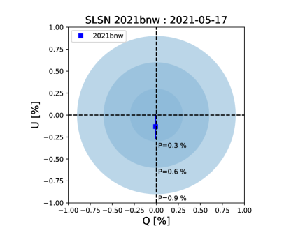
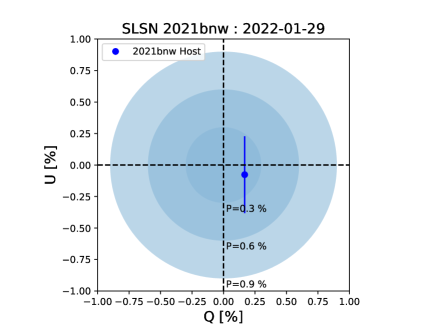
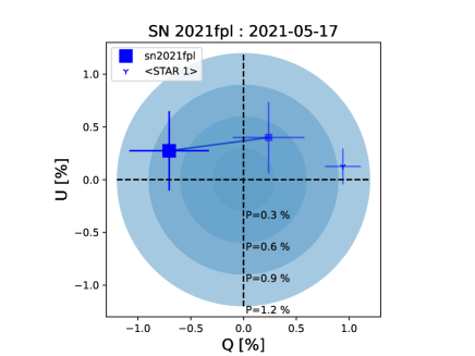
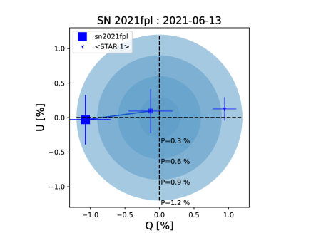
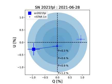
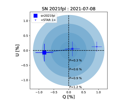
Figure 14: First row from top: SN 2021bnw (left) and its host (right), in the $Q-U$ plane, in the plane-of-sky reference frame after instrumental polarization ($IP$) and zero polarization angle ($ZPA$) corrections without Interstellar Polarization (ISP) correction. Concentric discs show polarization degrees ranges up to 0.3 $\%$, 0.6 $\%$ and 0.9 $\%$. Second and third row from top: SN 2020fpl ISP corrected $Q-U$ estimates have been obtained after subtraction of the $IP$, $ZPA$ corrected STAR 1 $Q-U$ estimate averaged over the four epochs (see Section 4.3 and Table 3 for details). The final values are shown with the double sized square symbols. The double sized square symbols are connected to the half translucent square symbols to show the effect of the ISP correction in the $Q-U$ plane. Concentric discs show polarization degrees ranges up to 0.3 $\%$, 0.6 $\%$, 0.9 $\%$ and 1.2 $\%$.

References

- Anderson et al. (2018) Anderson J. P., et al., 2018, A&A, 620, A67
- Angus et al. (2019) Angus C. R., et al., 2019, MNRAS, 487, 2215
- Bailer-Jones et al. (2021) Bailer-Jones C. A. L., Rybizki J., Fouesneau M., Demleitner M., Andrae R., 2021, AJ, 161, 147
- Bellm et al. (2019) Bellm E. C., et al., 2019, PASP, 131, 018002
- Blanchard et al. (2020) Blanchard P. K., Berger E., Nicholl M., Villar V. A., 2020, ApJ, 897, 114
- Blondin & Tonry (2007) Blondin S., Tonry J. L., 2007, ApJ, 666, 1024
- Bradley et al. (2021) Bradley L., et al., 2021, astropy/photutils: 1.0.2, doi:10.5281/zenodo.4453725
- Brennan & Fraser (2022) Brennan S. J., Fraser M., 2022, arXiv e-prints, p. arXiv:2201.02635
- Brown et al. (2016) Brown P. J., et al., 2016, ApJ, 828, 3
- Chambers et al. (2016) Chambers K. C., et al., 2016, arXiv e-prints, p. arXiv:1612.05560
- Chatzopoulos et al. (2013) Chatzopoulos E., Wheeler J. C., Vinko J., et al. 2013, ApJ, 773, 76
- Chen (2021) Chen K.-J., 2021, International Journal of Modern Physics D, 30, 2130001
- Chen et al. (2017) Chen T. W., et al., 2017, A&A, 602, A9
- Chen et al. (2022a) Chen Z. H., et al., 2022a, arXiv e-prints, p. arXiv:2202.02059
- Chen et al. (2022b) Chen Z. H., et al., 2022b, arXiv e-prints, p. arXiv:2202.02060
- Cikota et al. (2018) Cikota A., et al., 2018, MNRAS, 479, 4984
- Deckers et al. (2021a) Deckers M., Prentice S., Maguire K., Dimitriadis G., Magee M., Harvey L., Terwel J., 2021a, Transient Name Server AstroNote, 136, 1
- Deckers et al. (2021b) Deckers M., Prentice S., Maguire K., Dimitriadis G., Magee M., Harvey L., Terwel J., 2021b, Transient Name Server Classification Report, 2021-1365, 1
- Dessart (2019) Dessart L., 2019, A&A, 621, A141
- Dexter & Kasen (2013) Dexter J., Kasen D., 2013, ApJ, 772, 30
- Eftekhari et al. (2019) Eftekhari T., Berger E., Margalit B., et al. 2019, ApJ, 876, L10
- Eftekhari et al. (2021) Eftekhari T., Margalit B., Omand C. M. B., et al. 2021, ApJ, 912, 21
- Fremling (2021) Fremling C., 2021, Transient Name Server Discovery Report, 2021-326, 1
- Gal-Yam (2019) Gal-Yam A., 2019, ApJ, 882, 102
- Guillochon et al. (2018) Guillochon J., Nicholl M., Villar V. A., Mockler B., Narayan G., Mandel K. S., Berger E., Williams P. K. G., 2018, ApJS, 236, 6
- Heiles (2000) Heiles C., 2000, AJ, 119, 923
- Higson et al. (2019) Higson E., Handley W., Hobson M., Lasenby A., 2019, Statistics and Computing, 29, 891
- Hoflich (1991) Hoflich P., 1991, A&A, 246, 481
- Howell (2017) Howell D. A., 2017, in Alsabti A. W., Murdin P., eds, , Handbook of Supernovae. Springer International Publishing, p. 431, doi:10.1007/978-3-319-21846-5_41
- Inserra et al. (2013) Inserra C., Smartt S. J., Jerkstrand A., et al. 2013, ApJ, 770, 128
- Inserra et al. (2016) Inserra C., Bulla M., Sim S. A., Smartt S. J., 2016, ApJ, 831, 79
- Jerkstrand et al. (2017) Jerkstrand A., et al., 2017, ApJ, 835, 13
- Kangas et al. (2022) Kangas T., Yan L., Schulze S., et al. 2022, MNRAS, 516, 1193
- Kasen & Bildsten (2010) Kasen D., Bildsten L., 2010, ApJ, 717, 245
- Kasen et al. (2011) Kasen D., Woosley S. E., Heger A., 2011, ApJ, 734, 102
- Könyves-Tóth (2022) Könyves-Tóth R., 2022, arXiv e-prints, p. arXiv:2210.02153
- Könyves-Tóth & Vinkó (2021) Könyves-Tóth R., Vinkó J., 2021, ApJ, 909, 24
- Könyves-Tóth et al. (2020) Könyves-Tóth R., Thomas B. P., Vinkó J., Wheeler J. C., 2020, ApJ, 900, 73
- Kotera et al. (2013) Kotera K., Phinney E. S., Olinto A. V., 2013, MNRAS, 432, 3228
- Kumar et al. (2020) Kumar A., et al., 2020, ApJ, 892, 28
- Kumar et al. (2021) Kumar A., Kumar B., Pandey S. B., et al. 2021, MNRAS, 502, 1678
- Law et al. (2019) Law C. J., Omand C. M. B., Kashiyama K., et al. 2019, ApJ, 886, 24
- Lee (2019) Lee C.-H., 2019, ApJ, 875, 121
- Lee (2020) Lee C.-H., 2020, Astronomische Nachrichten, 341, 651
- Leloudas et al. (2015) Leloudas G., et al., 2015, ApJ, 815, L10
- Leloudas et al. (2017a) Leloudas G., et al., 2017a, ApJ, 837, L14
- Leloudas et al. (2017b) Leloudas G., et al., 2017b, ApJ, 843, L17
- Leloudas et al. (2022) Leloudas G., et al., 2022, Nature Astronomy, 6, 1193
- Liljegren et al. (2022) Liljegren S., Jerkstrand A., Barklem P. S., et al. 2022, arXiv e-prints, p. arXiv:2203.07021
- Lin et al. (2020) Lin W. L., et al., 2020, MNRAS, 497, 318
- Magee et al. (2021) Magee M., Terwel J., Prentice S., Harvey L., Strotjohann N. L., 2021, Transient Name Server Classification Report, 2021-338, 1
- Maund et al. (2019) Maund J. R., Steele I., Jermak H., Wheeler J. C., Wiersema K., 2019, MNRAS, 482, 4057
- Maund et al. (2020) Maund J. R., Leloudas G., Malesani D. B., Patat F., Sollerman J., de Ugarte Postigo A., 2020, MNRAS, 498, 3730
- Maund et al. (2021) Maund J. R., et al., 2021, MNRAS, 503, 312
- Metzger et al. (2014) Metzger B. D., Vurm I., Hascoët R., et al. 2014, MNRAS, 437, 703
- Moriya et al. (2018) Moriya T. J., Sorokina E. I., Chevalier R. A., 2018, Space Sci. Rev., 214, 59
- Murase et al. (2015) Murase K., Kashiyama K., Kiuchi K., et al. 2015, ApJ, 805, 82
- Murase et al. (2021) Murase K., Omand C. M. B., Coppejans D. L., et al. 2021, MNRAS, 508, 44
- Nicholl (2021) Nicholl M., 2021, arXiv e-prints, p. arXiv:2109.08697
- Nicholl et al. (2013) Nicholl M., et al., 2013, Nature, 502, 346
- Nicholl et al. (2016) Nicholl M., et al., 2016, ApJ, 826, 39
- Nicholl et al. (2017a) Nicholl M., Berger E., Margutti R., et al. 2017a, ApJ, 835, L8
- Nicholl et al. (2017b) Nicholl M., Berger E., Margutti R., Blanchard P. K., Guillochon J., Leja J., Chornock R., 2017b, ApJ, 845, L8
- Nicholl et al. (2017c) Nicholl M., Guillochon J., Berger E., 2017c, ApJ, 850, 55
- Omand & Jerkstrand (2022) Omand C. M. B., Jerkstrand A., 2022, arXiv e-prints, p. arXiv:2211.04502
- Omand et al. (2018) Omand C. M. B., Kashiyama K., Murase K., 2018, MNRAS, 474, 573
- Omand et al. (2019) Omand C. M. B., Kashiyama K., Murase K., 2019, MNRAS, 484, 5468
- Onken et al. (2019) Onken C. A., et al., 2019, Publ. Astron. Soc. Australia, 36, e033
- Piascik et al. (2014) Piascik A. S., Steele I. A., Bates S. D., Mottram C. J., Smith R. J., Barnsley R. M., Bolton B., 2014, in Ramsay S. K., McLean I. S., Takami H., eds, Society of Photo-Optical Instrumentation Engineers (SPIE) Conference Series Vol. 9147, Ground-based and Airborne Instrumentation for Astronomy V. p. 91478H, doi:10.1117/12.2055117
- Planck Collaboration et al. (2020) Planck Collaboration et al., 2020, A&A, 641, A1
- Poidevin et al. (2022) Poidevin F., Omand C. M. B., Pérez-Fournon I., et al. 2022, MNRAS, 511, 5948
- Pursiainen et al. (2022) Pursiainen M., et al., 2022, arXiv e-prints, p. arXiv:2202.01635
- Pursiainen et al. (2023) Pursiainen M., et al., 2023, arXiv e-prints, p. arXiv:2301.08111
- Quimby et al. (2018) Quimby R. M., et al., 2018, ApJ, 855, 2
- Rau et al. (2009) Rau A., et al., 2009, PASP, 121, 1334
- Saito et al. (2020) Saito S., et al., 2020, ApJ, 894, 154
- Silverman et al. (2015) Silverman J. M., Vinkó J., Marion G. H., Wheeler J. C., Barna B., Szalai T., Mulligan B. W., Filippenko A. V., 2015, MNRAS, 451, 1973
- Smartt et al. (2017) Smartt S. J., et al., 2017, Nature, 551, 75
- Smith et al. (2019) Smith K. W., et al., 2019, Research Notes of the American Astronomical Society, 3, 26
- Speagle (2020) Speagle J. S., 2020, MNRAS, 493, 3132
- Steele et al. (2004) Steele I. A., et al., 2004, in Oschmann Jacobus M. J., ed., Society of Photo-Optical Instrumentation Engineers (SPIE) Conference Series Vol. 5489, Ground-based Telescopes. pp 679–692, doi:10.1117/12.551456
- Suzuki & Maeda (2021) Suzuki A., Maeda K., 2021, ApJ, 908, 217
- Tanaka et al. (2017) Tanaka M., Maeda K., Mazzali P. A., et al. 2017, ApJ, 837, 105
- Taylor (2005) Taylor M. B., 2005, in Shopbell P., Britton M., Ebert R., eds, Astronomical Society of the Pacific Conference Series Vol. 347, Astronomical Data Analysis Software and Systems XIV. p. 29
- Terwel et al. (2021) Terwel J., et al., 2021, Transient Name Server AstroNote, 51, 1
- Thomas et al. (2011) Thomas R. C., Nugent P. E., Meza J. C., 2011, PASP, 123, 237
- Tonry et al. (2018) Tonry J. L., et al., 2018, PASP, 130, 064505
- Tonry et al. (2021) Tonry J., et al., 2021, Transient Name Server Discovery Report, 2021-771, 1
- Vurm & Metzger (2021) Vurm I., Metzger B. D., 2021, ApJ, 917, 77
- Wang et al. (1997) Wang L., Wheeler J. C., Höflich P., 1997, ApJ, 476, L27
- Wang et al. (2015) Wang S. Q., et al., 2015, ApJ, 799, 107
- Woosley (2010) Woosley S. E., 2010, ApJ, 719, L204
- Yaron & Gal-Yam (2012) Yaron O., Gal-Yam A., 2012, PASP, 124, 668