compat=1.1.0

Dynamics of the pseudo-FIMP in presence of a thermal dark matter

Abstract

In a two-component dark matter (DM) set up, when DM₁ is in equilibrium with the thermal bath, the other DM₂ can be equilibrated just by sizeable interaction with DM₁, even without any connection with the visible-sector particles. We show that such DM candidates (DM₂) have unique ‘freeze-out’ characteristics impacting the relic density, direct and collider search implications, and propose to classify them as ‘pseudo-FIMP’ (pFIMP). The dynamics of pFIMP is studied in a model-independent manner by solving generic coupled Boltzmann Equations (cBEQ), followed by a concrete model illustration.

Albeit tantalizing astrophysical and cosmological evidences, what constitutes the dark matter (DM) component of the universe remains a mystery with no direct experimental evidence in terrestrial experiments so far. Amongst DM geneses, thermal freeze-out of Weakly Interacting Massive Particle (WIMP) [1, 2] and non-thermal freeze-in of Feebly Interacting Massive Particle (FIMP) [3] can both address the observed DM relic density $\rm\Omega_{\rm DM}h^{2}\sim 0.12\pm.0012$ [4] with widely different interaction strengths with the Standard Model (SM) particles. Multipartite dark sectors offer interesting cosmological and phenomenological consequences, like modified freeze-out [32], relieving direct search constraints [6], addressing small scale structure anomalies of the universe [7] etc. The distinguishability of a two-component WIMP scenario, from that of single-component one, in terms of a double-hump in the missing energy distribution at collider [9, 8] or a kink in the recoil energy spectrum [10, 11] of the direct search experiment have been studied.

When the interaction between a WIMP and a FIMP remains ‘feeble’, the FIMP continues to be out of equilibrium [12, 13, 14], but enhanced interaction (of weak strength) can make the FIMP equilibrate to thermal bath and undergo freeze-out with some unique features, which are essentially model-independent, but relies on the properties of its thermal DM partner. We propose to classify such a particle into a category called ‘pseudo-FIMP’ (pFIMP), as it is a thermal DM in spite of having feeble connection with the SM. Also, pFIMP can be realized in presence of any thermal DM like Strongly Interacting Massive Particle (SIMP), independent of the depletion mechanism. Some model-dependent studies which mimic a pFIMP-like situation, have been studied [17, 32, 15, 34], but without elaborating the generic features that such particles possess. This letter illustrates the pFIMP characteristics in a model-independent way followed by a concrete model illustration and detection possibilities. Actually the idea of pFIMP has been conceptualised and demonstrated here for the first time, that occurs in a particular limit of the DM-DM and DM-SM interactions in a multicomponent set up. This leads to several model possibilities to be explored in the pFIMP limit as detailed in [18].

The evolution of DM number density in WIMP-FIMP framework is governed by a set of coupled Boltzmann equations (cBEQ) as shown in Eq. (4), in terms of yield ($Y=\frac{n}{s}$) as a function of $x=\mu_{12}/T$, where $\mu_{12}=m_{1}m_{2}/\left(m_{1}+m_{2}\right)$ denotes the reduced mass of the two DMs, and $T$ denotes the temperature of the thermal bath.

$$\begin{split}\frac{dY_{1}}{dx}=&-\frac{{s}}{x~{}H(x)}\Biggl{[}\langle\sigma v\rangle_{11\rightarrow\rm{SM}}\Bigl{(}Y_{1}^{2}-Y_{1}^{\rm{eq}^{2}}\Bigr{)}\\ &+\langle\sigma v\rangle_{11\rightarrow 22}\Bigl{(}Y_{1}^{2}-\frac{Y_{1}^{\rm eq^{2}}}{Y_{2}^{\rm eq^{2}}}Y_{2}^{2}\Bigr{)}\Biggr{]},\\ \frac{dY_{2}}{dx}=&\frac{2~{}{s}}{x~{}H(x)}\Biggl{[}\dfrac{1}{{s}}\langle\Gamma_{\rm SM\rightarrow 22}\rangle(Y_{\rm SM}^{\rm eq}-\frac{Y_{2}^{2}}{Y_{2}^{\rm eq^{2}}}Y_{\rm SM}^{\rm eq})\\ &+\langle\sigma v\rangle_{\rm{SM}\rightarrow 22}\Bigl{(}Y_{\rm SM}^{\rm eq^{2}}-\frac{Y_{2}^{2}}{Y_{2}^{\rm eq^{2}}}Y_{\rm SM}^{\rm eq^{2}}\Bigr{)}\\ &+\langle\sigma v\rangle_{11\rightarrow 22}\Bigl{(}Y_{1}^{2}-\frac{Y_{1}^{\rm eq^{2}}}{Y_{2}^{\rm eq^{2}}}Y_{2}^{2}\Bigr{)}\Biggr{]}\,.\end{split}$$ (1)

In the above equation, ${s}\,=\,\frac{2\pi^{2}}{45}g_{*}^{{s}}\left(\frac{\mu_{12}}{x}\right)^{3}~{},~{}H(x)\,=\,1.67\sqrt{g_{*}^{\rho}}{\mu^{2}_{12}}x^{-2}\rm M_{pl}^{-1}$. Subscripts $1,~{}2$ in Eq. (4) and in the rest of the draft denote WIMP and FIMP (pFIMP) components respectively. Interactions that crucially determine the DM densities are WIMP depletion to SM governed by $\langle\sigma v\rangle_{11\rightarrow\rm{SM}}$, FIMP production from the SM bath via annihilation $\langle\sigma v\rangle_{\rm{SM}\rightarrow 22}$ and/or decay $\langle\Gamma_{\rm SM\rightarrow 22}\rangle$, and WIMP-FIMP conversion $\langle\sigma v\rangle_{11\rightarrow 22}$ ($\langle..\rangle$ denotes thermal average and $v$ is M$\ddot{o}$llar velocity). The cBEQ for a two component WIMP case is also the same as Eq. 4. The difference lies in the $(i)$ strength of the DM-SM interactions; $\langle\sigma v\rangle_{\tt{\tt WIMP}}\sim 10^{-8}~{}{\rm GeV}^{-2}$, whereas $\langle\sigma v\rangle_{\tt{\tt FIMP}}\sim 10^{-20}~{}{\rm GeV}^{-2}$ and $(ii)$ initial conditions, $Y_{\tt{\tt WIMP}}|_{x\sim 0}=Y^{\rm eq}\sim x^{3/2}e^{-x}$, $Y_{\tt{\tt FIMP}}|_{x\sim 0}=0$. In the following, the conversion $\langle\sigma v\rangle_{11\rightarrow 22}$ is varied from ‘feeble’ to ‘weak’ strength to show the transition from FIMP to pFIMP state. Other notations in Eq. (4) are all standard and available in any DM text [6].

For solving Eq. (4) to obtain DM yields in a model-independent way, we choose some benchmark values of the DM masses and $\langle\sigma v\rangle$. As the temperature dependence in $\langle\sigma v\rangle$ requires $\sigma(s)$ ($s$ is c.o.m energy) i.e. diagrams that contribute to annihilation, in absence of which we assume here $\langle\sigma v\rangle\approx\sigma^{\rm T}$; a temperature-independent threshold value representing $(\sigma v)$ at the freeze-out (freeze-in) temperature for WIMP/pFIMP (FIMP). Full $\langle\sigma v\rangle$ is used for a model-specific analysis and the dynamical features remain the same.

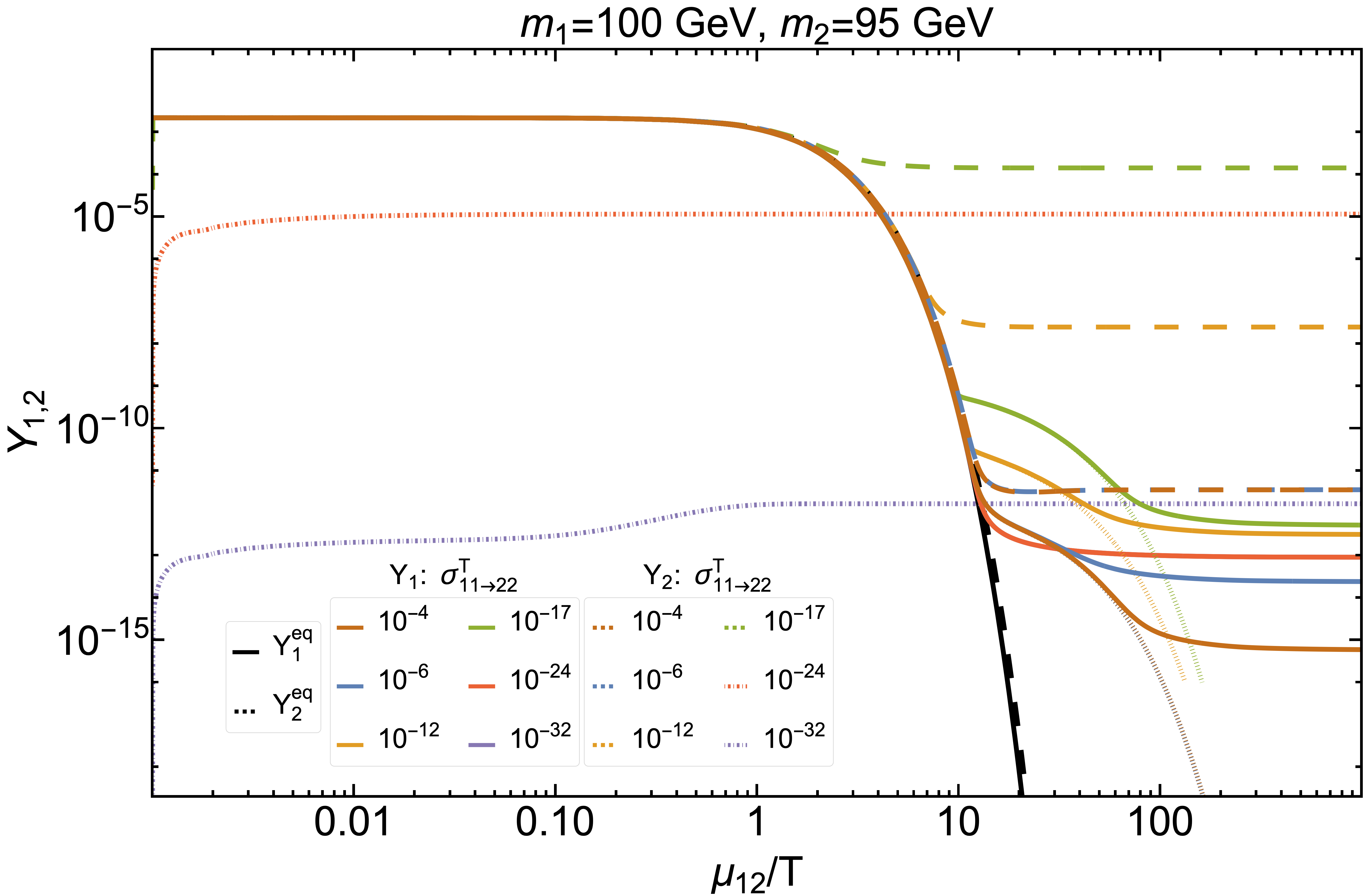
1a 

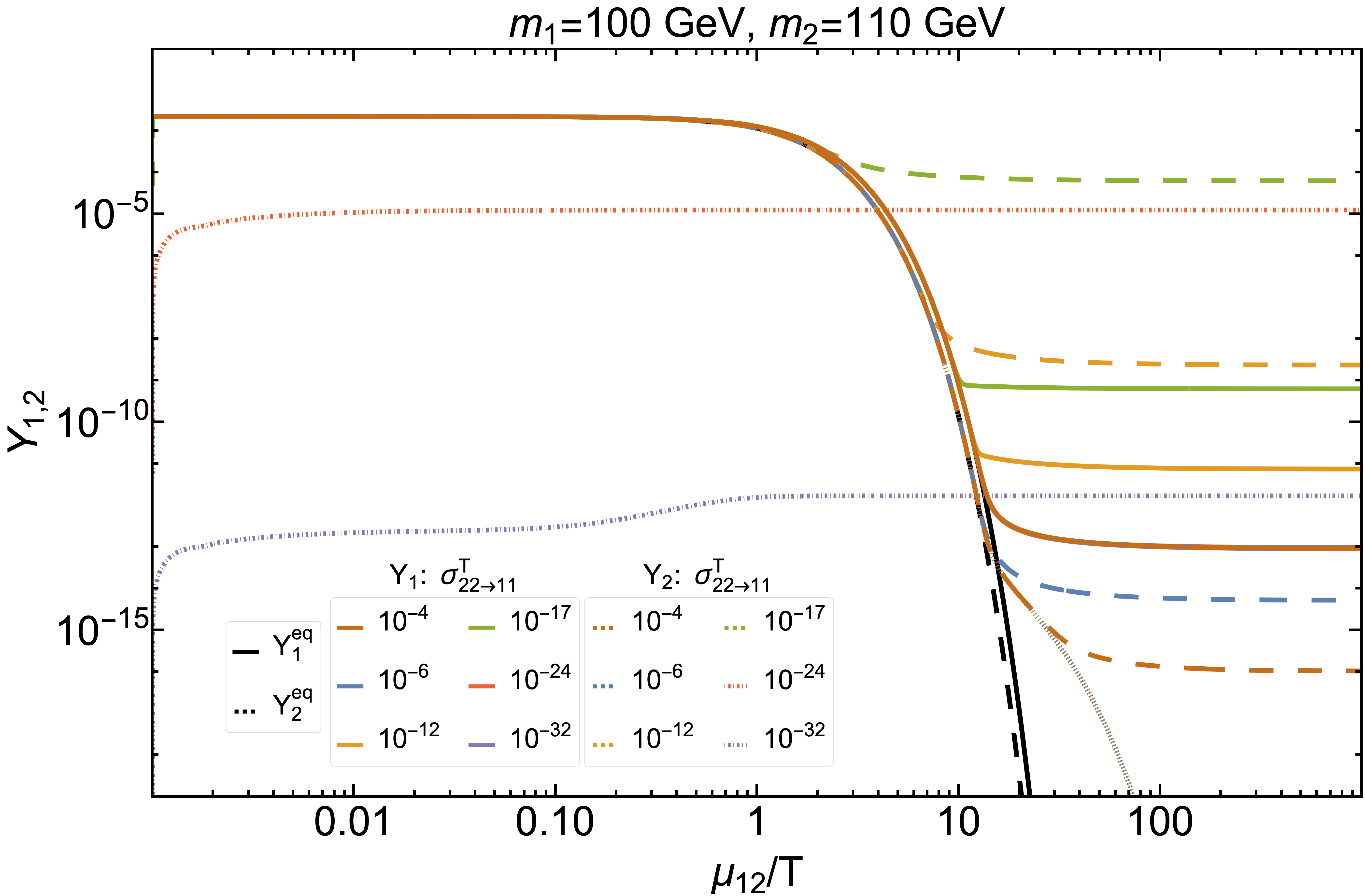
1b 

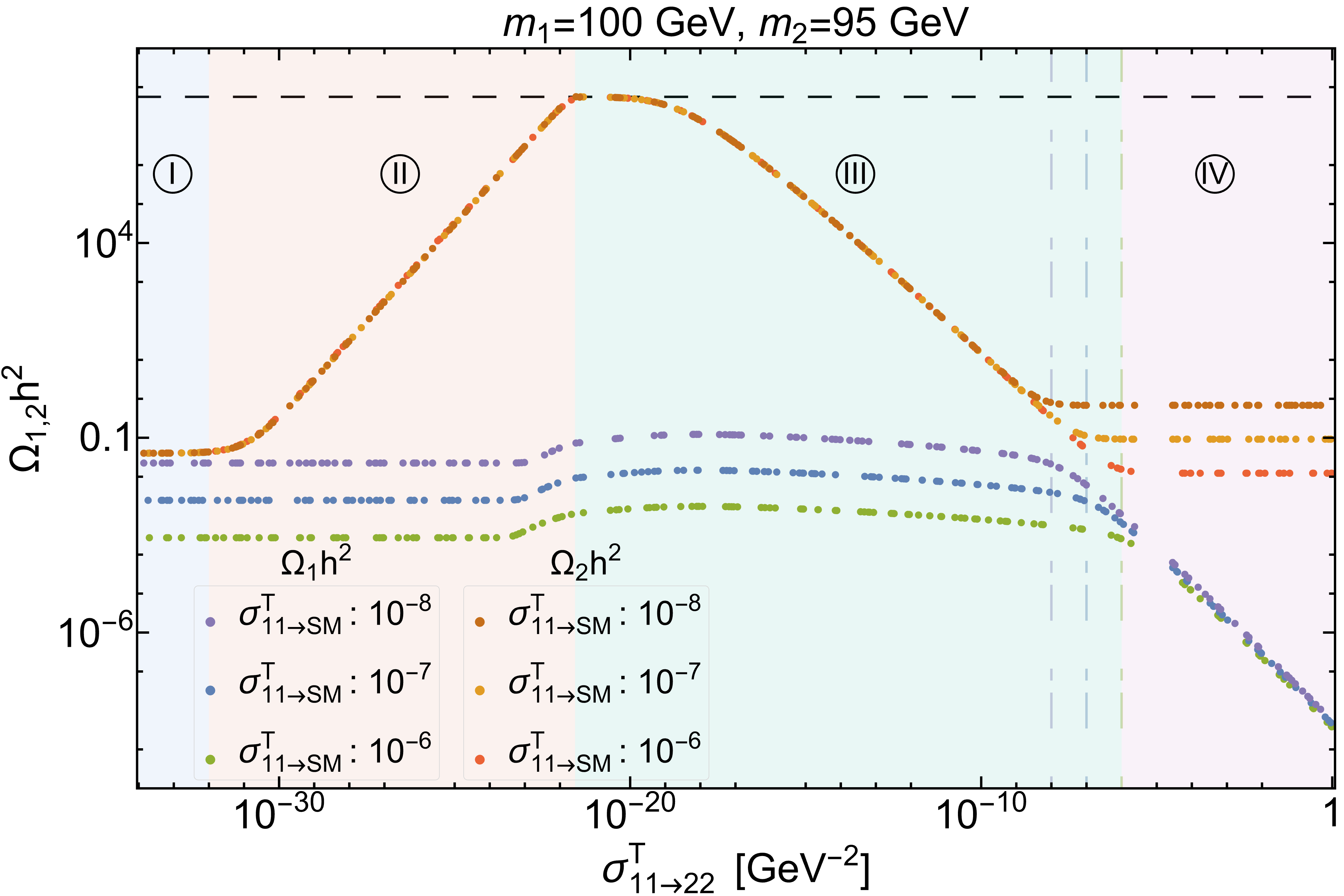
1c 

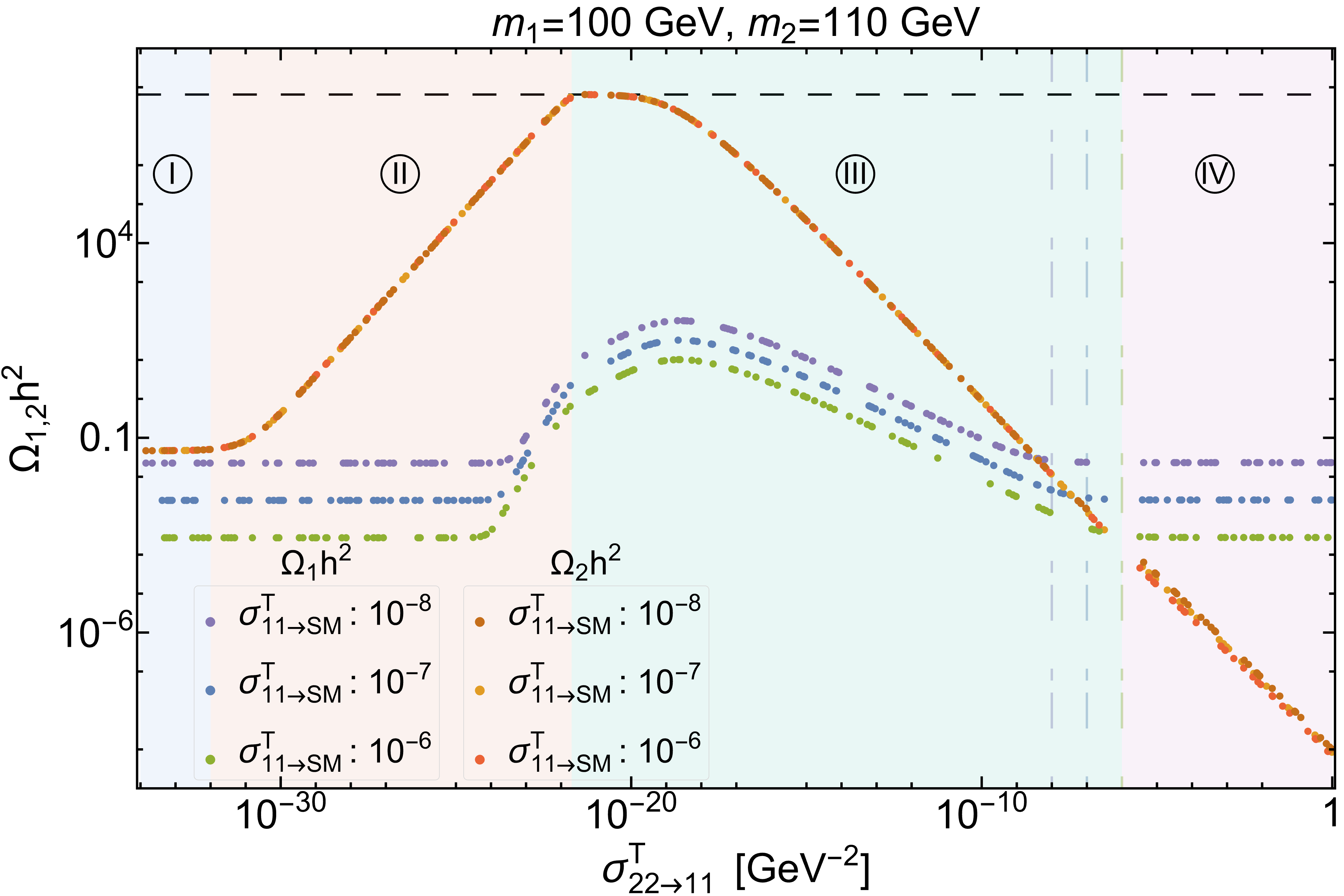
1d 

Figure 1: (a) $Y_{1,2}(x)$ for mass hierarchy 1, where solid (dotted) [dashed] curves denote WIMP (FIMP) [pFIMP] with equilibrium distributions marked in black; (b) Same as (a) for hierarchy 2; (c) ${\rm\Omega_{1,2}h^{2}}$ as a function of $\sigma^{\rm T}_{11\rightarrow 22}$ for hierarchy 1; red/yellow/orange dotted lines represent FIMP(pFIMP), while green/blue/pink ones represent WIMP; (d) same as (c) for hierarchy 2. For all the plots $\rm~{}\Gamma^{T}_{SM\rightarrow 22}=10^{-23}GeV^{-1}$, $\rm~{}\sigma^{\rm T}_{SM\rightarrow 22}=10^{-32}GeV^{-2}$. For upper panel plots, we choose $\rm\sigma^{T}_{11\rightarrow SM}=10^{-7}GeV^{-2}$. See figure inset/caption for other parameters kept fixed.

Plots in fig. 1 summarise the main outcome of the model independent analysis. In figures 1, 1, $Y_{1,2}$ are plotted as a function of $x$, for different conversion rates. In figures 1, 1, ${\rm{\Omega_{1,2}h^{2}}}$ are plotted as a function of $\sigma^{\rm T}_{11\rightarrow 22}$ (left), $\sigma^{\rm T}_{22\rightarrow 11}$ (right). Note, that $\langle\sigma v\rangle_{11\rightarrow 22}=\langle\sigma v\rangle_{22\rightarrow 11}\rm(Y_{2}^{eq}/Y_{1}^{eq})^{2}$. All the cross-sections are in the units of GeV^-2 and in the following text we may omit writing it explicitly. Both the mass hierarchies (1) $m_{1}>m_{2}$ (on left) and (2) $m_{1}<m_{2}$ (on right) are shown. In hierarchy (1), conversion from WIMP to pFIMP is kinematically allowed, while the reverse process is Boltzmann suppressed ($\sim e^{-2\delta m~{}x},~{}\delta m=m_{1}-m_{2}$). For hierarchy (2), its the other way round. The whole analysis can be divided into four different regions of varying conversion cross-section, : $\sigma^{\rm T}_{11\rightarrow 22}<\sigma^{\rm T}_{\rm{SM}\rightarrow 22}$, : $\sigma^{\rm T}_{\rm{SM}\rightarrow 22}\lesssim\sigma^{\rm T}_{11\rightarrow 22}\ll\sigma^{\rm T}_{11\rightarrow\rm{SM}}$, : $\sigma^{\rm T}_{\rm{SM}\rightarrow 22}\ll\sigma^{\rm T}_{11\rightarrow 22}<\sigma^{\rm T}_{11\rightarrow\rm{SM}}$, : $\sigma^{\rm T}_{11\rightarrow\rm{SM}}\lesssim\sigma^{\rm T}_{11\rightarrow 22}$, as shown by the colour bars in figs. 1, 1.

In region , when the conversion rate is very small ($\sigma^{\rm T}_{11\rightarrow 22}\sim 10^{-32}$) it has no role in FIMP or WIMP relic density. The FIMP remains out-of-equilibrium and freeze-in occurs via $\sigma^{\rm T}_{\rm{SM}\rightarrow 22},\Gamma^{\rm T}_{\rm SM\rightarrow 22}$, see the blue dotted lines in figs. 1, 1 and horizontal red/yellow/orange dotted lines in figs. 1, 1.

In region , when $\sigma^{\rm T}_{11\rightarrow 22}\gtrsim\sigma^{\rm T}_{\rm{SM}\rightarrow 22}$, the FIMP is still out of equilibrium but the freeze-in is guided by the conversion process, see the red dotted lines in figs. 1, 1 ($\sigma^{\rm T}_{11\rightarrow 22}\sim 10^{-24}$) and the growing red/yellow/orange dotted lines with larger $\sigma^{\rm T}_{11\rightarrow 22}$ in figs. 1, 1. The WIMP still remains unaffected, evident from the red/violet solid lines in figs. 1, 1, and horizontal blue/green/violet dotted lines in figs. 1, 1.

In region , as the conversion rate $\sigma^{\rm T}_{11\rightarrow 22}$ is increased further, the FIMP starts following the thermal distribution, see green ($\sigma^{\rm T}_{11\rightarrow 22}=10^{-17}$) and orange ($\sigma^{\rm T}_{11\rightarrow 22}=10^{-12}$) dashed lines in figs. 1, 1. This is when the FIMP turns into pFIMP and undergoes “freeze-out”. Larger conversion cross-section keeps pFIMP longer in the thermal bath resulting smaller relic density; see the steady decline in red/yellow/orange dotted lines with larger $\sigma^{\rm T}_{11\rightarrow 22}(\approx 10^{-17}$) in figs. 1, 1. Notably, the freeze-out point of pFIMP is governed purely by its conversion rate from (to) the WIMP. However, the WIMP freeze-out is additionally dictated by $\sigma^{\rm T}_{11\rightarrow\rm SM}$. Therefore pFIMP always decouples before or together with the WIMP (compare dashed and solid lines in figs. 1, 1) and provides an important difference between WIMP-WIMP and pFIMP-WIMP case. For heavier WIMP (hierarchy 1), the WIMP freeze-out shows a bump (see fig. 1), as it attains a modified equilibrium distribution following Eq. (2), after pFIMP decouples [32],

$$\rm n_{1}^{\rm eq^{\prime}}=n_{1}^{\rm eq}\left(\frac{\sigma^{T}_{11\rightarrow SM}+\sigma^{T}_{11\rightarrow 22}\left(n_{2}/n_{2}^{eq}\right)^{2}}{\sigma^{T}_{11\rightarrow SM}+\sigma^{T}_{11\rightarrow 22}}\right)^{1/2}\,.$$ (2)

When pFIMP is heavier (hierarchy 2), the conversion from WIMP to pFIMP is kinematically suppressed, and no modified freeze-out pattern for WIMP is observed (see fig. 1). This provides another distinction of pFIMP-WIMP scenario from the WIMP-WIMP one. After FIMP equilibrates to thermal bath, larger production of WIMP from pFIMP enhances WIMP relic density, see the jump from red thick line ($\sigma^{\rm T}_{11\rightarrow 22}=10^{-24}$) to green thick line ($\sigma^{\rm T}_{11\rightarrow 22}=10^{-17}$) in figs. 1, 1. This feature is also observed in the violet/blue/green dashed lines in figs 1, 1. For hierarchy (1), the departure of the WIMP from the original equilibrium distribution to modified equilibrium (Eq. 2) depends on $\sigma^{\rm T}_{11\rightarrow 22}$ (compare green and orange thick lines in fig. 1), however the freeze-out from modified equilibrium is primarily governed by $\sigma^{\rm T}_{11\rightarrow\rm SM}$, yielding same $\Omega_{1}{\rm h}^{2}$ for different $\sigma^{\rm T}_{11\rightarrow 22}$. On the contrary, for hierarchy (2), when pFIMP is heavier, the WIMP production from pFIMP is substantial due to kinematic accessibility, as a result the WIMP freeze out is delayed, and the WIMP yield goes down with enhanced conversion rate (see fig. 1), providing a crucial hierarchical distinction.

In region , with $\sigma^{\rm T}_{11\rightarrow 22}>\sigma^{\rm T}_{11\rightarrow\rm{SM}}$, we see even more interesting consequences. For hierarchy (1), the WIMP relic density falls drastically with larger $\sigma^{\rm T}_{11\rightarrow 22}$ due to larger depletion (violet/green/blue dotted lines in fig. 1), while the pFIMP yield remains the same, and is dependent only on $\sigma^{\rm T}_{11\rightarrow\rm SM}$ (horizontal brown/yellow/red dotted lines in fig. 1, or overlapping dashed lines in fig. 1 for $\sigma^{\rm T}_{11\rightarrow 22}=10^{-6},10^{-4}$). This is because pFIMP yield in hierarchy (1) is governed by two quantities, WIMP number density and conversion rate. Now, the WIMP number density falls with larger $\sigma^{\rm T}_{11\rightarrow 22}$, while that is compensated by the enhanced production via $\sigma^{\rm T}_{11\rightarrow 22}$ which keeps the pFIMP yield almost constant in this region. For hierarchy (2), the situation is however different. With increasing conversion, pFIMP yield decreases significantly, while the WIMP yield remains almost constant (see fig. 1). This is attributed again to the combined effect of decreasing pFIMP number density along with larger WIMP production from pFIMP with larger conversion rate. Since pFIMP has no SM interaction, it goes out of the original equilibrium distribution as WIMP freezes out. However, due to considerable conversion to WIMP, it achieves a modified equilibrium distribution as seen from the orange and blue dashed lines in fig. 1.

$\rm DM_{1}-DM_{2}$	$\langle\sigma v_{\rm SM-DM_{1}}\rangle$	$\langle\sigma v_{\rm SM-DM_{2}}\rangle$	$\langle\sigma v_{\rm DM_{1}-DM_{2}}\rangle$	Observed Relic	Direct-Detection	Indirect-Detection
WIMP-WIMP	Weak	Weak	Weak/Feeble	Yes [6]	Yes-Yes [22, 6]	Yes-Yes[23]
WIMP-pFIMP	Weak	Feeble	Weak	Yes [32, 34]	Yes-Yes[32]	Yes-Yes
FIMP-FIMP	Feeble	Feeble	Weak/Feeble	Yes [20, 21, 7]	No-No [7]	No-No

Table 1: Generic two-component DM scenarios, order of the interaction with SM as well as between DMs, possibilities of satisfying relic abundance and being probed in direct (indirect) search experiments.

Figure 2: Relic density allowed points in the $\sigma^{\rm T}_{11\rightarrow{\rm SM}}-\sigma^{\rm T}_{22\rightarrow 11}$ plane for $m_{2}>m_{1}$ in WIMP-pFIMP limit. $\delta m=|m_{1}-m_{2}|$ is varied as shown in the colour-bar. We choose $\Gamma_{{\rm SM}\rightarrow 22}^{{\rm T}}=10^{-20}$ GeV${}^{-1},~{}\sigma^{\rm T}_{{\rm SM}\rightarrow 22}=10^{-30}$ GeV^-2, $m_{1}=100$ GeV and decaying particle mass $\rm m_{s}=300$ GeV.

We now perform a model-independent scan of the WIMP-pFIMP parameter space, where we assume that annihilation cross-sections and masses have adequate freedom to be varied independently. In fig. 2, we scan points that satisy relic density ($\rm\Omega_{1}h^{2}+\Omega_{2}h^{2}=0.12\pm.0012$) in $\sigma^{\rm T}_{11\rightarrow\rm{SM}}-\sigma^{\rm T}_{22\rightarrow 11}$ plane for hierarchy (2). WIMP mass is kept fixed at $100~{}\rm GeV$ and the mass splitting between WIMP and pFIMP $\delta m=|m_{1}-m_{2}|$ is varied as shown in the colour bar. When the conversion rate is small, $\sigma^{\rm T}_{11\rightarrow\rm{SM}}$ requires to be large in order to achieve WIMP density within the limit. Understandably $\delta m$ does not play a major role here, and a large range of $\delta m$ is allowed (right side of fig. 2). With larger conversion rate, smaller $\sigma^{\rm T}_{11\rightarrow\rm{SM}}$ is required (left of fig. 2). If we decrease $\sigma^{\rm T}_{11\rightarrow\rm{SM}}$ keeping $\sigma^{\rm T}_{22\rightarrow 11}$ fixed, the WIMP tends to become overabundant, unless the conversion contribution from pFIMP to WIMP is decreased by increasing $\delta m$ via Boltzmann suppression. However, for hierarchy (1), the situation is different and the whole $\sigma^{\rm T}_{11\rightarrow\rm{SM}}-\sigma^{\rm T}_{11\rightarrow 22}$ parameter space within $\delta m=|m_{1}-m_{2}|\lesssim 10$ GeV becomes allowed.

In summary, the allowed points accommodate mostly small mass difference ($\delta m\lesssim 10$ GeV) and the mass hierarchy between WIMP and pFIMP play a crucial role in the consequent DM phenomenology, absent in usual WIMP-WIMP set up. Here we have ensured that the conversion cross-section remains well below the bullet cluster observational data [19] that suggests the upper limit on the self-interaction cross-section of DM(s) per unit mass to be, $\rm{\sigma/m<0.7~{}cm^{2}g^{-1}\sim 3.2\times 10^{3}~{}GeV^{-3}}$.

In Table 1, we depict a few examples of two component DM scenarios, with their strength of DM-DM conversion, possibility of producing correct relic abundance, along with direct (indirect) detection prospects at present/future experiments. Generically, the pFIMP detection is heavily dependent on the detection prospects of the WIMP, as the pFIMP direct search or collider search signal proceeds via WIMP loop as shown in Fig. 3. The strength of the pFIMP interaction is less than the WIMP, but can be of similar order when the loop factor is compensated by the large pFIMP-WIMP interaction.

We would now like to validate our claims of pFIMP characteristics for a specific model. Here we use temperature dependent $\langle\sigma v\rangle$ in terms of the model parameters. We choose the simplest model consisting of two real scalar singlets, where $\phi_{1}$ behaves as WIMP and $\phi_{2}$ as FIMP/(pFIMP), both of which are rendered stable under $\mathbb{Z}_{2}\otimes\mathbb{Z}^{\prime}_{2}$ symmetry. The Lagrangian density is given by,

$$\begin{split}\mathcal{L}&=\mathcal{L}_{\rm SM}+\frac{1}{2}\partial_{\mu}\phi_{1}\partial^{\mu}\phi_{1}-\frac{1}{2}\mu_{\phi_{1}}^{2}\phi_{1}^{2}-\frac{1}{4!}\rm\lambda_{\phi_{1}}\phi_{1}^{4}-\frac{1}{2}\lambda_{1H}\phi_{1}^{2}H^{\dagger}H\\ +&\rm\frac{1}{2}\partial_{\mu}\phi_{2}\partial^{\mu}\phi_{2}-\frac{1}{2}\mu_{\phi_{2}}^{2}\phi_{2}^{2}-\frac{1}{4!}\lambda_{\phi_{2}}\phi_{2}^{4}-\frac{1}{2}\lambda_{2H}\phi_{2}^{2}H^{\dagger}H-\frac{1}{4}\lambda_{12}\phi_{1}^{2}\phi_{2}^{2}\,.\end{split}$$ (3)

This model in WIMP-WIMP limit has been explored in many texts including [6]. Here we focus on the pFIMP regime, partly explored in [34]. For that, we choose $\phi_{2}$ to have negligible coupling with the SM, $\rm\lambda_{2H}\approx 10^{-12}$. However, in presence of the WIMP-like $\phi_{1}$, the conversion governed by $\lambda_{12}$ plays a key role and with large $\lambda_{12}\sim 1$ it reproduces all the characteristics of pFIMP. Relic density as a function of $\lambda_{12}$ is plotted in the supplementary material, which shows similar features to that of figs. 1, 1 and validates the pFIMP characteristics. The WIMP-pFIMP limit of this model has also been verified with the code micrOMEGAs4.1 [24].

Direct search of pFIMP is possible via WIMP loop, absent a tree-level connection to SM. The Feynman graph is shown in fig. 3, while the detailed calculations are provided in the supplementary material.

Figure 3: A schematic Feynman diagram for collider (left) and direct-detection (right) of pFIMP via one-loop WIMP interaction.

Figure 4: Relic density allowed points of the model described by Eq. 3 in $\sigma_{{\phi_{1}}_{\rm eff}}^{\rm SI}-m_{\phi_{1}}$ plane. The parameters varied are $\{m_{\phi_{2}},\lambda_{\rm 1H},\lambda_{12}\}$. $\sigma_{{\phi_{2}}_{\rm eff}}^{\rm SI}$ is shown in colour bar. See heading and figure inset for other parameters and experimental limits.

${\rm m_{\phi_{1}}[GeV]}$	${\rm m_{\phi_{2}}[GeV]}$	$\lambda_{\rm 1H}$	$\lambda_{\rm 12}$	$\rm loop~{}factor$	${\rm\Omega_{\phi_{1}}h^{2}}$	${\rm\Omega_{\phi_{2}}h^{2}}$	$\sigma^{\rm SI}_{{\phi_{1}}_{\rm eff}}[{\rm cm^{2}}]$	$\sigma^{\rm SI}_{{\phi_{2}}_{\rm eff}}[{\rm cm^{2}}]$	Gluon fusion (fb)
									WIMP	pFIMP
63.33	60.50	0.10	4	$2.53\times 10^{-3}$	0.0002	0.1203	$3.3\times 10^{-47}$	$5.0\times 10^{-48}$	8.4	13.9
104.1	100.0	0.22	6	$8.40\times 10^{-3}$	0.0002	0.1210	$7.89\times 10^{-47}$	$2.15\times 10^{-47}$	0.69	1.18 $\times 10^{-3}$
405.0	402.9	0.30	8	$1.52\times 10^{-2}$	0.0101	0.1091	$4.06\times 10^{-46}$	$7.49\times 10^{-48}$	9$\times 10^{-4}$	2.34 $\times 10^{-6}$

Table 2: Some benchmarks for the two-component scalar singlet model (Eq. (3)) in WIMP-pFIMP limit, where the loop factor is approximated as $\sim(\lambda_{\rm 1H}\lambda_{12})/(16\pi^{2})$. The last two columns depict the WIMP and pFIMP production cross-section at LHC via Gluon fusion yielding mono-jet+$\not{E_{T}}$ in the final state at $\sqrt{s}=14~{}\rm TeV$.

Large WIMP-pFIMP interaction ($\lambda_{12}$) helps in the detection of pFIMP, the loop suppression factor $\sim 1/(16\pi^{2})$ allows it to evade existing bound and make it accessible to future sensitivities. In fig. 4, spin-independent (SI) direct detection cross-section for the WIMP ($\phi_{1}$) and pFIMP $(\phi_{2})$ is shown as a function of WIMP mass for relic density allowed points of the model. The sensitivity of existing direct search data have all been compared [25, 28, 26, 27]. A clear dip is seen in the resonance region $m_{\phi_{1}}\sim m_{h}/2$, where due to resonance enhancement $\lambda_{\rm 1H}$ is relaxed and points satisfy direct search constraints. One should however remember the limitations of Lee-Weinberg mechanism in the vicinity of resonance as pointed out by [29, 30].

When $m_{\phi_{1}}>m_{\phi_{2}}$, small $\delta m$ enhances the $\phi_{1}\phi_{1}\rightarrow\phi_{2}\phi_{2}$ conversion, consequently decreasing $\Omega_{\phi_{1}}$ and effective direct detection cross-section $\sigma^{\rm SI}_{i_{\rm eff}}=\frac{\Omega_{i}}{\Omega_{\rm tot}}\sigma^{\rm SI}_{i}$, where $i=\{\phi_{1},\phi_{2}\}$. However, most of the parameter space of this WIMP-pFIMP limit of the two component scalar DM model is on the verge of exclusion by the LZ (2022) data, leaving the Higgs resonance, $m_{\phi_{1}}\sim m_{h}$ regions and some points close to the $\pm 1\sigma$ exclusion limit up to 500 GeV survive to be explored. Unlike WIMP-WIMP case, where two DMs may have widely different masses, pFIMP limit necessitates the mass splitting to be small and therefore serves as a guiding principle for searching both DM components. Similarly pFIMPs can also be produced in collider via one-loop WIMP graphs yielding mono-X plus missing energy signals as estimated in the Table 2 for some benchmark points where the model satisfies relic density and direct search bounds. In this case, detection of pFIMP seems only possible in the resonance region, owing to a resonant enhancement in the production. Interesting to note that, even in this region, the effective coupling between Higgs and pFIMP is rather small due to loop suppression, thereby making it safe from the Higgs invisible decay constraints. One can have plethora of other possibilities, like a fermion WIMP instead of a scalar WIMP, which enhances the detection possibility of a scalar pFIMP, see for example, [18]. We again note here that the model chosen for illustration is not the best for detection, rather it is the simplest one.

Furthermore, pFIMP having a similar mass to that of the WIMP provides a challenge in distinguishing the DM components in direct and collider searches, as the distinguishability (a kink in the recoil spectrum for direct search [10, 11] or two bumps in missing energy at colliders [9, 8]) often depends on the mass splitting of the DM components. However mono-X signal can be useful, as the position of the peak here primarily depends on the operator structure, angular momentum conservation etc. We are exploring such possibilities, however the two component scalar case will be difficult to disentangle.

Finally we summarise here. We have shown that the FIMP can reach equilibrium in presence of a thermal DM component and sizeable conversion cross-section. We call it pFIMP. The freeze-out of pFIMP precedes that of its thermal partner and requires a small mass splitting with it. The numerical solution of Eq. 4 presented here and approximate analytical solution provided in the supplementary material validates all the pFIMP properties in a model independent way. The pFIMP realization in presence of SIMP is also provided in the supplementary material. The freeze-out properties of pFIMP is verified for the simplest two-component DM model with two scalar singlets. The detection prospect of pFIMP via WIMP loop in future direct, indirect and collider search experiments opens up new possibilities. Such investigations in context of direct DM search for two-component WIMP-pFIMP model has been pursued in [18].

Acknowledgments:— SB and JL acknowledge the grant CRG/2019/004078 from SERB, Govt. of India. DP thanks University Grants Commission for senior research fellowship and Heptagon, IITG for useful discussions.

SUPPLEMENTAL MATERIAL

Appendix A Semi-analytic solution of the cBEQ for WIMP-pFIMP scenario

A two-component WIMP-pFIMP framework is governed by a coupled Boltzmann equations (cBEQ),

$$\begin{split}\frac{dY_{1}}{dx}=-\frac{2\pi^{2}\rm{M_{pl}}}{45\times 1.67}\frac{g_{\star}^{s}}{\sqrt{g_{\star}^{\rho}}}\frac{\mu_{12}}{x^{2}}&\Biggl{[}\langle\sigma v\rangle_{11\rightarrow\rm{SM}}\Bigl{(}Y_{1}^{2}-Y_{1}^{\rm{eq}^{2}}\Bigr{)}+\langle\sigma v\rangle_{11\rightarrow 22}\Bigl{(}Y_{1}^{2}-\frac{Y_{1}^{\rm eq^{2}}}{Y_{2}^{\rm eq^{2}}}Y_{2}^{2}\Bigr{)}\Biggr{]},\\ \frac{dY_{2}}{dx}=\frac{2\rm{M_{pl}}}{1.67\times\sqrt{g_{\star}^{\rho}}}\frac{x}{\mu_{12}^{2}}\langle\Gamma_{\rm SM\rightarrow 22}\rangle(Y_{\rm SM}^{\rm eq}-\frac{Y_{2}^{2}}{Y_{2}^{\rm eq^{2}}}Y_{\rm SM}^{\rm eq})+&\frac{4\pi^{2}\rm{M_{pl}}}{45\times 1.67}\frac{g_{\star}^{s}}{\sqrt{g_{\star}^{\rho}}}\frac{\mu_{12}}{x^{2}}\Biggl{[}\langle\sigma v\rangle_{\rm{SM}\rightarrow 22}\Bigl{(}Y_{\rm SM}^{\rm eq^{2}}-\frac{Y_{2}^{2}}{Y_{2}^{\rm eq^{2}}}Y_{\rm SM}^{\rm eq^{2}}\Bigr{)}+\langle\sigma v\rangle_{11\rightarrow 22}\Bigl{(}Y_{1}^{2}-\frac{Y_{1}^{\rm eq^{2}}}{Y_{2}^{\rm eq^{2}}}Y_{2}^{2}\Bigr{)}\Biggr{]}\,.\end{split}$$ (4)

We elaborate upon the semi analytical solution of the cBEQ as in Eq. 4 in WIMP-pFIMP limit, for both the hierarchies:

• Case-I: WIMP mass $>$ pFIMP mass (i.e. $m_{1}>m_{2}$).

• Case-II: WIMP mass $<$ pFIMP mass (i.e. $m_{1}<m_{2}$).

The methodology follows the procedure in [32].

A.1 Case-I ($m_{1}>m_{2}$)

In WIMP-pFIMP limit, we neglect the pFIMP production from the visible sector as the pFIMP coupling with SM is very small, compared to the conversion cross-section. So, in the following we consider, $\Gamma_{\rm SM\rightarrow 22}=\langle\sigma v\rangle_{\rm{SM}\rightarrow 22}=0$. For notational ease, let us also use, $\rm\langle\sigma v\rangle_{11\rightarrow SM}=\sigma_{1},~{}\langle\sigma v\rangle_{11\rightarrow 22}=\sigma_{12},~{}\langle\sigma v\rangle_{22\rightarrow 11}=\sigma_{21}$, $\rm[(2\pi^{2}\sqrt{g_{\star}^{\rho}})/(45\times 1.66)]M_{pl}=n_{f}$ with Planck mass $\rm M_{pl}=1.22\times 10^{19}$ GeV. Recall that $\sigma_{12}=\sigma_{21}\left(n_{2}^{eq}/{n_{1}^{eq}}\right)^{2}$. With above, the cBEQ in terms of bath temperature $(T)$ becomes,

$$\begin{split}&\frac{dY_{1}}{dT}=n_{f}\left[\sigma_{1}\left(Y_{1}^{2}-Y_{1}^{\rm eq^{2}}\right)+\sigma_{12}\left(Y_{1}^{2}-\frac{Y_{1}^{\rm eq^{2}}}{Y_{2}^{\rm eq^{2}}}Y_{2}^{2}\right)\right]\,,\\ &\frac{dY_{2}}{dT}=-2n_{f}\left[\sigma_{12}\left(Y_{1}^{2}-\frac{Y_{1}^{\text{eq}^{2}}}{Y_{2}^{\text{eq}^{2}}}Y_{2}^{2}\right)\right]\,.\end{split}$$ (5)

The equilibrium yield is given by Maxwell-Boltzmann distribution,

$$Y_{i}^{\rm eq}\left(T\right)=0.145\frac{g}{g_{\star}^{s}}\left(\frac{m_{i}}{T}\right)^{3/2}\exp\left(-\frac{m_{i}}{T}\right)=A_{i}T^{-3/2}e^{-m_{i}/T}~{}\text{with}~{}A_{i}=0.145\frac{g}{g_{\star}^{s}}m_{i}^{3/2}\,.$$

Defining $Y_{1}^{eq^{2}}\left(\frac{\sigma_{1}}{\sigma_{1}+\sigma_{12}}+\frac{\sigma_{12}}{\sigma_{1}+\sigma_{12}}\frac{Y_{2}^{2}}{Y_{2}^{eq^{2}}}\right)=y_{1}^{eq^{2}}$, Equation 5 becomes,

$$\begin{split}&\frac{dY_{1}}{dT}=n_{f}\left(\sigma_{1}+\sigma_{12}\right)\left(Y_{1}^{2}-y_{1}^{\rm eq^{2}}\right)\,,\\ &\frac{dY_{2}}{dT}=-2n_{f}\left[\sigma_{12}\left(Y_{1}^{2}-\frac{Y_{1}^{\text{eq}^{2}}}{Y_{2}^{\text{eq}^{2}}}Y_{2}^{2}\right)\right]\,.\end{split}$$ (6)

In order to solve the cBEQ analytically, it would be convenient to divide this whole scenario in three regions on the bath temperature: Region A: $T\gg T_{f_{i}}$, Region B: $T\simeq T_{f_{i}}$ and Region C: $T\ll T_{f_{i}}$ where $T_{f_{i}}$ denotes the freeze-out temperature of both species $i=1,2$. Let use consider the difference of DM yield from equilibrium yield as $\Delta_{1}=Y_{1}-y_{1}^{\rm eq}$ and $\Delta_{2}=Y_{2}-Y_{2}^{\rm eq}$. Using these relations, Equation 6 becomes,

$$\begin{split}&\frac{d\Delta_{1}}{dT}+\frac{dy_{1}^{eq}}{dT}=n_{f}\left(\sigma_{1}+\sigma_{12}\right)\left(\Delta_{1}^{2}+2\Delta_{1}y_{1}^{\rm eq}\right)\,,\\ &\frac{d\Delta_{2}}{dT}+\frac{dY_{2}^{eq}}{dT}=-2n_{f}\sigma_{12}\Bigl{[}\left(\Delta_{1}+y_{1}^{\rm eq}\right)^{2}-\frac{Y_{1}^{\rm eq^{2}}}{Y_{2}^{\rm eq^{2}}}\left(\Delta_{2}+Y_{2}^{\rm eq}\right)^{2}\Bigr{]}\,.\end{split}$$ (7)

$\bullet$ Region A:

For $T\gg T_{f_{i}}$, $\frac{d\Delta_{i}}{dT}$ is negligible and Equation 7 becomes,

$$\frac{dy_{1}^{eq}}{dT}=n_{f}\left(\sigma_{1}+\sigma_{12}\right)\left(\Delta_{1}^{2}+2\Delta_{1}y_{1}^{\rm eq}\right)\,,$$ (8)

$$\frac{dY_{2}^{eq}}{dT}=-2n_{f}\sigma_{12}\Bigl{[}\left(\Delta_{1}+y_{1}^{\rm eq}\right)^{2}-\frac{Y_{1}^{\rm eq^{2}}}{Y_{2}^{\rm eq^{2}}}\left(\Delta_{2}+Y_{2}^{\rm eq}\right)^{2}\Bigr{]}\,.$$ (9)

$\bullet$ Region B:

Let us suppose $T_{f_{2}}>T_{f_{1}}$, then both Equation 8 and Equation 9 hold at $T_{f_{2}}$, but only Equation 8 holds at $T_{f_{1}}$ as pFIMP already freezes out at $T_{f_{1}}$. In the vicinity of $T\simeq T_{f}$, we may further assume $\Delta_{1}(T_{f_{1}})=c_{1}y_{1}^{eq}(T_{f_{1}})$ and $\Delta_{2}(T_{f_{2}})=c_{2}Y_{2}^{eq}(T_{f_{2}})$ [31], where $c_{i}$’s are unknown constants whose values are determined by matching the analytical result with the numerical one. Substituting in Equation 8 and Equation 9, we get,

$$y_{1}^{eq^{\prime}}(T_{f_{1}})\approx n_{f}\left(\sigma_{1}+\sigma_{12}\right)c_{1}(c_{1}+2)y_{1}^{eq^{2}}(T_{f_{1}})\,,$$ (10)

$$2n_{f}(\sigma_{1}+\sigma_{12})\sigma_{12}\left[\left(c_{2}+1\right)^{2}Y_{1}^{eq^{2}}(T_{f_{2}})-y_{1}^{eq^{2}}(T_{f_{2}})\right]\approx(\sigma_{1}+\sigma_{12})Y_{2}^{eq^{\prime}}(T_{f_{2}})+2\sigma_{12}y_{1}^{eq^{\prime}}(T_{f_{2}})\,.$$ (11)

In the above,

$$Y_{i}^{\rm eq^{\prime}}(T) =\left(-\frac{3}{2T}+\frac{m_{i}}{T^{2}}\right)Y_{i}^{\rm eq}(T)\,,$$ (12)

$$y_{1}^{eq^{2}}(T_{f_{2}}) =Y_{1}^{eq^{2}}(T_{f_{2}})\left(\frac{\sigma_{1}}{\sigma_{1}+\sigma_{12}}+\frac{\sigma_{12}}{\sigma_{1}+\sigma_{12}}\left(c_{2}+1\right)^{2}\right)\,,$$ (13)

$$y_{1}^{eq^{2}}(T_{f_{1}}) =Y_{1}^{eq^{2}}(T_{f_{1}})\left(\frac{\sigma_{1}}{\sigma_{1}+\sigma_{12}}+(c_{2}+1)^{2}\frac{\sigma_{12}}{\sigma_{1}+\sigma_{12}}\frac{Y_{2}^{eq^{2}}(T_{f_{2}})}{Y_{2}^{eq^{2}}(T_{f_{1}})}\right)\,,$$ (14)

$$y_{1}^{eq^{\prime}}(T_{f_{2}}) =\frac{Y_{1}^{eq^{2}}(T_{f_{2}})}{y_{1}^{eq}(T_{f_{2}})}\left[\left(-\frac{3}{2T_{f_{2}}}+\frac{m_{1}}{T_{f_{2}}^{2}}\right)\left(\frac{\sigma_{1}}{\sigma_{1}+\sigma_{12}}+\frac{\sigma_{12}}{\sigma_{1}+\sigma_{12}}\left(c_{2}+1\right)^{2}\right)-\left(-\frac{3}{2T_{f_{2}}}+\frac{m_{2}}{T_{f_{2}}^{2}}\right)\frac{\sigma_{12}}{\sigma_{1}+\sigma_{12}}c_{2}\left(c_{2}+1\right)\right]\,,$$ (15)

$$y_{1}^{eq^{\prime}}(T_{f_{1}}) =\frac{Y_{1}^{eq^{2}}(T_{f_{1}})}{y_{1}^{eq}(T_{f_{1}})}\left[\left(-\frac{3}{2T_{f_{1}}}+\frac{m_{1}}{T_{f_{1}}^{2}}\right)\frac{\sigma_{1}}{\sigma_{1}+\sigma_{12}}+\frac{\sigma_{12}}{\sigma_{1}+\sigma_{12}}\left(c_{2}+1\right)^{2}\frac{m_{1}-m_{2}}{T_{f_{1}}^{2}}\left(\frac{T_{f_{1}}}{T_{f_{2}}}\right)^{3}e^{-2\frac{m_{2}}{T_{f_{2}}}}e^{2\frac{m_{2}}{T_{f_{1}}}}\right]\,.$$ (16)

Equation 10 and Equation 11 can be written further as,

$$y_{1}^{eq^{\prime}}(T_{f_{1}})=n_{f}\left(\sigma_{1}+\sigma_{12}\right)c_{1}(c_{1}+2)y_{1}^{eq^{2}}(T_{f_{1}})\,,$$ (17)

$$P~{}T_{f_{2}}^{-1/2}=2\sigma_{12}QT_{f_{2}}e^{\frac{m_{1}}{T_{f_{2}}}}+(\sigma_{1}+\sigma_{12})\left(-\frac{3}{2}+\frac{m_{2}}{T_{f_{2}}}\right)\left(\frac{m_{2}}{m_{1}}\right)^{3/2}e^{2\frac{m_{1}}{T_{f_{2}}}}e^{-\frac{m_{2}}{T_{f_{2}}}}\,;$$ (18)

where,

$$P=2A_{1}n_{f}\sigma_{1}\sigma_{12}c_{2}\left(c_{2}+2\right)\,,$$ (19)

$$Q=\left[\left(-\frac{3}{2T_{f_{2}}}+\frac{m_{1}}{T_{f_{2}}^{2}}\right)\left(\frac{\sigma_{1}}{\sigma_{1}+\sigma_{12}}+\frac{\sigma_{12}}{\sigma_{1}+\sigma_{12}}\left(c_{2}+1\right)^{2}\right)-\left(-\frac{3}{2T_{f_{2}}}+\frac{m_{2}}{T_{f_{2}}^{2}}\right)\frac{\sigma_{12}}{\sigma_{1}+\sigma_{12}}c_{2}\left(c_{2}+1\right)\right]\left[\frac{\sigma_{1}}{\sigma_{1}+\sigma_{12}}+\frac{\sigma_{12}}{\sigma_{1}+\sigma_{12}}\left(c_{2}+1\right)^{2}\right]^{-\dfrac{1}{2}}\,.$$ (20)

Equation 17 and Equation 18 are transcendental equations, analytical solutions are difficult to obtain, but using numerical method it is possible to extract the values of freeze out temperature $T_{f_{1}}$ and $T_{f_{2}}$, which we did.

$\bullet$ Region C:

When $T\ll T_{f_{i}},$ then, $Y_{i}^{\rm eq},~{}Y_{i}^{\rm eq^{\prime}}$ and $\frac{Y_{1}^{eq^{2}}}{Y_{2}^{eq^{2}}}$ are exponentially suppressed, so, $\Delta_{i}\gg Y_{i}^{\rm eq}$ and Equation 7 becomes,

$$\frac{d\Delta_{1}}{dT}\approx n_{f}(\sigma_{1}+\sigma_{12})\Delta_{1}^{2}\,,$$ (21)

$$\frac{d\Delta_{2}}{dT}\approx-2n_{f}\sigma_{12}\Delta_{1}^{2}\,.$$ (22)

After solving the differential equations between $T_{f_{i}}$ to $T$ with $\Delta_{i}(T)\gg\Delta_{i}(T_{f_{i}})$, we get,

$$\Delta_{1}(T)\approx\left[\frac{1}{\Delta_{1}(T_{f_{1}})}+n_{f}(\sigma_{1}+\sigma_{12})\left(T_{f_{1}}-T\right)\right]^{-1}\,,$$ (23)

$$\Delta_{2}(T)\approx\Delta_{2}(T_{f_{2}})-2n_{f}\sigma_{12}(T-T_{f_{2}})\left[\left(\frac{1}{\Delta_{1}(T_{f_{1}})}+n_{f}(\sigma_{1}+\sigma_{12})(T_{f_{1}}-T)\right)\left(\frac{1}{\Delta_{1}(T_{f_{1}})}+n_{f}(\sigma_{1}+\sigma_{12})(T_{f_{1}}-T_{f_{2}})\right)\right]^{-1}\,.$$ (24)

Following, $\Delta_{1}(T_{f_{1}})\approx c_{1}y_{1}^{\rm eq}(T_{f_{1}})$, $\Delta_{2}(T_{f_{2}})\approx c_{2}Y_{2}^{\rm eq}(T_{f_{2}})$, at $T=T_{\rm CMB}=2.35\times 10^{-13}\rm GeV$, the DM yields are,

$$\Delta_{1}(T_{\rm CMB})\approx Y_{1}(T_{\rm CMB})\approx\left(\frac{1}{\Delta_{1}(T_{f_{1}})}+n_{f}(T_{f_{1}}-T_{\rm CMB})(\sigma_{1}+\sigma_{12})\right)^{-1}\,,$$ (25)

$$\Delta_{2}(T_{\rm CMB})\approx Y_{2}(T_{\rm CMB})\approx\Delta_{2}(T_{f_{2}})+2n_{f}\sigma_{12}\int_{T_{\rm CMB}}^{T_{f_{2}}}\Delta_{1}^{2}(T)~{}dT\,.$$ (26)

Figure 5: Analytic solution of the cBEQ (represented by thick line) and numerical solution (represented by points) of Eq. (4) for pFIMP-WIMP case is shown as a function of conversion cross-section. The unknown constants are chosen as $c_{1}=2$ and $c_{2}=7$. Vertical dot-dashed line corresponding to $\sigma_{12}=\sigma_{1}$.

Figure 6: In-equilibrium $\rm(\Gamma>H)$ (green shade) and out-of-equilibrium $\rm(\Gamma<H)$ (yellow shade) possibilities for pFIMP. Green line corresponds to $\rm\Gamma(T)=H(T)$ and red star corresponds to $\rm T=T_{RH}$. Both mass hierarchies $m_{1}>m_{2}$ (left), $m_{2}>m_{1}$ (right) are plotted.

Using the analytical approximate solutions, relic density as a function of conversion cross-section for both WIMP and pFIMP have been shown in Figure 5. They show reasonably good agreement, the tiny mismatch with numeric result at low and high conversion region is only due to the entropy d.o.f $(g_{*}^{s})$ and matter d.o.f $(g_{*}^{\rho})$ which depends on temperature (specifically $T\lesssim 5\rm~{}GeV$) but for simplicity we have neglected this temperature dependence and chosen a fixed value of $g_{*}^{\rho}=g_{*}^{s}\simeq 75$ for the semi analytical solution.

In the similar way it is easy to evaluate the present DM relic for the inverse mass hierarchy ($m_{1}<m_{2}$) where one necessary input is $T_{f_{1}}>T_{f_{2}}$ and $\Delta_{2}(T_{f_{2}})=c_{2}y_{2}^{eq}(T_{f_{2}})$ with $y_{2}^{eq}=Y_{1}\frac{Y_{2}^{eq}}{Y_{1}^{eq}}$. The transition of FIMP into a pFIMP depends not only on the temperature but also on the interaction rate. This can be understood, just by analysing the relation between interaction rate ($\Gamma$) and Hubble expansion rate ($H$). Figure 6 depicts it for both mass hierarchies: $m_{1}>m_{2}$ (left), $m_{2}>m_{1}$ (right). $\rm\Gamma\simeq H$ has been represented by the green curve. The red star points correspond to ${\rm\Gamma(T\sim T_{RH})=H(T\sim T_{RH})}$ in both the figures. In our model-independent analysis, we have neglected the temperature dependence of the conversion cross-section, which may alter the high temperature behaviour of the plot.

Appendix B Dynamics of the pFIMP in presence of a SIMP

The pFIMP behaviour could also be achieved in presence of SIMP [33] when DM-DM conversion is sufficiently large ($\sim$ weak scale). The cBEQ for pFIMP-SIMP scenario can be written as:

$$\frac{dY_{\rm w}}{dx}= \frac{2~{}\bf{s}}{x~{}H(x)}\left[\frac{1}{\textbf{s}}\left(Y_{\rm SM}^{\rm eq}-Y_{\rm SM}^{\rm eq}\frac{Y_{\rm w}^{2}}{Y_{\rm w}^{\rm eq^{2}}}\right)\langle\Gamma\rangle_{\rm SM\rightarrow\rm w~{}w}\,+\,\Bigl{(}Y_{\rm SM}^{\rm eq^{2}}-Y_{\rm SM}^{\rm eq^{2}}\frac{Y_{\rm w}^{2}}{Y_{\rm w}^{\rm eq^{2}}}\Bigr{)}\langle\sigma v\rangle_{\rm{SM~{}SM}\rightarrow\rm w~{}w}+\Bigl{(}Y_{\rm s}^{2}-Y_{\rm s}^{\rm eq^{2}}\frac{Y_{\rm w}^{2}}{Y_{\rm w}^{\rm eq^{2}}}\Bigr{)}\langle\sigma v\rangle_{\rm s~{}s\rightarrow w~{}w}\right]\,,$$ (27)

$$\frac{dY_{\rm s}}{dx}= -\frac{\bf{s}}{x~{}H(x)}\bigg{[}\left(Y_{\rm s}^{2}-Y_{\rm s}^{\rm eq^{2}}\right)\langle\sigma v\rangle_{\rm s~{}s\rightarrow SM~{}SM}\,+\,\textbf{s}\left(Y_{\rm s}^{3}-Y_{\rm s}^{2}Y_{\rm s}^{\rm eq}\right)\langle\sigma v^{2}\rangle_{3s\rightarrow 2s}+\left(Y_{\rm s}^{2}-Y_{\rm s}^{\rm eq^{2}}\frac{Y_{\rm w}^{2}}{Y_{\rm w}^{\rm eq^{2}}}\right)\langle\sigma v\rangle_{\rm s~{}s\rightarrow w~{}w}\bigg{]}\,.$$ (28)

In the above subscripts $s$ denote SIMP and ${\rm w}$ denote pFIMP, $\mu=1/\left(\frac{1}{m_{\rm w}}+\frac{1}{m_{\rm s}}\right)^{-1},~{}x=\mu/T,~{}H(x)\,=\,1.67\sqrt{g_{*}^{\rho}}\mu^{2}x^{-2}\rm M_{pl}^{-1},~{}$$\bf{s}$$\,=\,\frac{2\pi^{2}}{45}g_{*}^{\rm\bf{s}}\left(\frac{\mu}{x}\right)^{3}$$,~{}\langle\sigma v\rangle_{\rm w~{}w\rightarrow s~{}s}\,=\,\langle\sigma v\rangle_{\rm s~{}s\rightarrow w~{}w}\left(Y_{\rm s}^{\rm eq}/Y_{\rm w}^{\rm eq}\right)^{2},~{}Y_{i}^{\rm eq}\,=\,\frac{45}{4\pi^{4}}\frac{g_{i}}{g_{*}^{\bf s}}\left(\frac{m_{i}}{\mu}x\right)^{2}K_{2}\left(\frac{m_{i}}{\mu}x\right)$. For simplicity we only have taken $3{\rm DM\rightarrow 2DM}$ depletion process for SIMP, but ${\rm(nDM\rightarrow 2DM}$ with $n>3)$ can also be taken to show the same effect. We solve the cBEQ with increasing order of conversion cross-section to show the change from FIMP to pFIMP case in Figure 7 for both mass hierarchies $m_{\rm w}>m_{\rm s}$ (left panel) and $m_{\rm w}<m_{\rm s}$ (right panel). The features remain very similar to pFIMP-WIMP scenario.

(a)

(b)

Figure 7: DM yield with $x=\mu/T$ in pFIMP-SIMP case for fixed DM masses and conversion cross-sections, where the black solid (dashed) curves denote equilibrium distribution for SIMP (pFIMP) corresponding to (a) $m_{\rm s}>m_{\rm w}$ and (b) $m_{\rm s}<m_{\rm w}$. For all the plots $\langle\sigma v\rangle_{\rm s~{}s\rightarrow SM~{}SM}\,=\,10^{-10}\rm GeV^{-2},$ $\rm\langle\Gamma\rangle_{SM\rightarrow\rm w~{}w}\,=\,10^{-23}\rm GeV^{-1},$ $\langle\sigma v\rangle_{\rm SM~{}SM\rightarrow\rm w~{}w}\,=\,10^{-32}\rm GeV^{-2}$ $\rm~{}and~{}m_{\rm SM}\,=\,10~{}GeV$ have been assumed.

Appendix C Solution to cBEQ for two component scalar DM model

(a)

(b)

Figure 8: Variation of relic density with $\lambda_{12}$ for the the two component scalar DM model, where $\phi_{1}$ is WIMP and $\phi_{2}$ is pFIMP for $m_{\phi_{1}}>m_{\phi_{2}}$ (a) and $m_{\phi_{1}}<m_{\phi_{2}}$ (b). See figure insets and headings for other parameters kept fixed for the plot.

In figure 8, we show the relic density of the DM components $\phi_{1},\phi_{2}$ for a two component scalar DM scenario, as a function of the DM-DM interaction coupling $\lambda_{12}$. Both the hierarchies $m_{\phi_{1}}>m_{\phi_{2}}$ (a) and $m_{\phi_{1}}<m_{\phi_{2}}$ (b) are shown. We see a spectacularly similar feature to that of model independent analysis presented in fig. 1 of the main text, showing that the generic properties assigned to pFIMP are generically valid.

Appendix D Direct search prospect of pFIMP via WIMP loop

+ +

Figure 9: The Feynman diagrams for pFIMP ($\phi_{2}$) to interact with SM via Higgs. Sum of these tree (left), 1-loop (middle) and counter (right) diagram gives the total renormalized $\lambda_{h\phi_{2}\phi_{2}}$ coupling at 1-loop level.

We will now provide the details of direct search prospect of the pFIMP ($\phi_{2}$) in the two component scalar singlet model. The renormalized amplitude is given by (see Figure 9),

$$\Gamma_{h\phi_{2}\phi_{2}} \,=\,\Gamma_{h\phi_{2}\phi_{2}}^{\rm tree}+\Gamma_{h\phi_{2}\phi_{2}}^{\rm 1-loop}+\Gamma_{h\phi_{2}\phi_{2}}^{\rm counter}\,,$$

$$\,=\,-i\lambda_{h\phi_{2}\phi_{2}}+\Gamma_{h\phi_{2}\phi_{2}}^{\rm 1-loop}-i\delta_{\lambda_{h\phi_{2}\phi_{2}}}\,.$$ (29)

Here,

$$\Gamma_{h\phi_{2}\phi_{2}}^{\rm 1-loop}\left(q_{h}\right)\,=\,\frac{1}{2}\mu^{4-d}\left(-i\lambda_{\phi_{1}\phi_{1}\phi_{2}\phi_{2}}\right)\left(-i\lambda_{h\phi_{1}\phi_{1}}\right)\int\frac{d^{d}k}{(2\pi)^{d}}\frac{i}{k^{2}-m_{\phi_{1}}^{2}}\frac{i}{(k-q_{h})^{2}-m_{\phi_{1}}^{2}}\,.$$ (30)

The transfer momentum $q_{h}$ is momentum transfer from initial to final state particles and $1/2$ is the symmetry factor due to the scalar loop. The dimension regularization parameter $\mu$ (mass scale) is introduced to keep couplings dimensionless in $d=4-2\epsilon$ dimension when $\epsilon\rightarrow 0_{+}$. Now the 1-loop amplitude in Equation 30 becomes,

$$\Gamma_{h\phi_{2}\phi_{2}}^{\rm 1-loop}\left(q_{h}^{2}\right)\,=\, \frac{1}{2}\left(-i\lambda_{\phi_{1}\phi_{1}\phi_{2}\phi_{2}}\right)\left(-i\lambda_{h\phi_{1}\phi_{1}}\right)\frac{-i}{16\pi^{2}}\int_{0}^{1}dx\left(\frac{4\pi\mu^{2}}{\Delta}\right)^{\epsilon}\Gamma\left(\epsilon\right)\hskip 28.45274pt{\rm where},~{}\Delta=m_{\phi_{1}}^{2}-x(1-x)q_{h}^{2}\,,$$

$$\,=\, \frac{1}{2}\left(-i\lambda_{\phi_{1}\phi_{1}\phi_{2}\phi_{2}}\right)\left(-i\lambda_{h\phi_{1}\phi_{1}}\right)\frac{-i}{16\pi^{2}}\int_{0}^{1}dx\left(\frac{1}{\epsilon}-\gamma_{E}+\ln\left[4\pi\mu^{2}\right]-\ln\left[\Delta\right]\right)\,,$$

$$\,=\, \frac{1}{2}\left(-i\lambda_{\phi_{1}\phi_{1}\phi_{2}\phi_{2}}\right)\left(-i\lambda_{h\phi_{1}\phi_{1}}\right)\frac{-i}{16\pi^{2}}\int_{0}^{1}dx\left(\frac{1}{\epsilon}-\gamma_{E}+\ln\left[4\pi\mu^{2}\right]-\ln\left[m_{\phi_{1}}^{2}-x(1-x)q_{h}^{2}\right]\right)\,.$$ (31)

Figure 10: Contour plot in $m_{\phi_{1}}-m_{\phi_{2}}$ plane to represent the absolute 1-loop amplitude $\rm|\Gamma_{h\phi_{2}\phi_{2}}^{{total}}|_{t\rightarrow 0}$ for some chosen values of $\lambda_{1H}$ and $\lambda_{12}$ as mentioned in the figure heading.

There is an ambiguity of choosing the renormalisation scale, its unknown essentially. The direct search cross-section depends on the choice. For, $q_{h}^{2}\rightarrow 0$, the cross-section is vanishingly small [34], however if we choose $q_{h}^{2}=4m_{\phi_{2}}^{2}$, a scale relevant for the pFIMP production, the contribution is substantial [35]. So we choose $q_{h}^{2}=4m_{\phi_{2}}^{2}$ as the renormalization condition setting point and calculate the counter term which removes the divergence from 1-loop amplitude $\Gamma_{h\phi_{2}\phi_{2}}^{\rm 1-loop}$ to yield,

$$\Gamma_{h\phi_{2}\phi_{2}}^{\rm total}\left(q_{h}^{2}\right)\,=\, -i\lambda^{\rm relic}_{h\phi_{2}\phi_{2}}-\frac{i}{32\pi^{2}}\left(\lambda_{\phi_{1}\phi_{1}\phi_{2}\phi_{2}}\lambda_{h\phi_{1}\phi_{1}}\right)\int_{0}^{1}dx\ln\left[\frac{m_{\phi_{1}}^{2}-x(1-x)4m_{\phi_{2}}^{2}}{m_{\phi_{1}}^{2}-x(1-x)q_{h}^{2}}\right]\,.$$ (32)

Therefore, using Equation 32 the effective spin-independent DM-nucleon direct-detection cross-section in zero transfer momentum $(q_{h}^{2}=t\rightarrow 0)$ limit turns out to be,

$$\sigma_{{\phi_{2}}_{\rm eff}}^{\rm SI}\,=\,\frac{\Omega_{\phi_{2}}h^{2}}{\Omega_{\phi_{1}}h^{2}+\Omega_{\phi_{2}}h^{2}}\frac{\mu_{n}^{2}m_{n}^{2}}{4\pi v^{2}m_{\phi_{2}}^{2}}\frac{f_{n}^{2}}{m_{h}^{4}}|\Gamma_{h\phi_{2}\phi_{2}}^{\rm total}|^{2}_{t\rightarrow 0}\,.$$ (33)

In the above, $\mu_{n}=\frac{m_{n}m_{\phi_{2}}}{m_{n}+m_{\phi_{2}}}$ where $m_{n}$ is the nucleon mass, $f_{n}=\frac{2}{9}+\frac{7}{9}\displaystyle\sum_{u,d,s}f_{T_{q}}^{n}$ with $f_{T_{u}}^{p(n)}=0.018(0.013),~{}f_{T_{d}}^{p(n)}=0.027(0.040),$ and $f_{T_{s}}^{p(n)}=0.037(0.037)$ [35]. We use Equation 33 for pFIMP direct search cross-section while scanning the parameter space as shown in the main text.

References

[1]
M. Kamionkowski and M. S. Turner,
Phys. Rev. D 42 (1990), 3310-3320
doi:10.1103/PhysRevD.42.3310
[2]
G. Jungman, M. Kamionkowski and K. Griest,
Phys. Rept. 267 (1996), 195-373
doi:10.1016/0370-1573(95)00058-5
[arXiv:hep-ph/9506380 [hep-ph]].
[3]
L. J. Hall, K. Jedamzik, J. March-Russell and S. M. West,
JHEP 03 (2010), 080
doi:10.1007/JHEP03(2010)080
[arXiv:0911.1120 [hep-ph]].
[4]
N. Aghanim et al. [Planck],
Astron. Astrophys. 641 (2020), A6
[erratum: Astron. Astrophys. 652 (2021), C4]
doi:10.1051/0004-6361/201833910
[arXiv:1807.06209 [astro-ph.CO]].
[5]
S. Bhattacharya, A. Drozd, B. Grzadkowski and J. Wudka,
JHEP 10 (2013), 158
doi:10.1007/JHEP10(2013)158
[arXiv:1309.2986 [hep-ph]].
[6]
S. Bhattacharya, P. Poulose and P. Ghosh,
JCAP 04 (2017), 043
doi:10.1088/1475-7516/2017/04/043
[arXiv:1607.08461 [hep-ph]].
[7]
P. Ghosh, P. Konar, A. K. Saha and S. Show,
JCAP 10 (2022), 017
doi:10.1088/1475-7516/2022/10/017
[arXiv:2112.09057 [hep-ph]].
[8]
S. Bhattacharya, P. Ghosh, J. Lahiri and B. Mukhopadhyaya,
[arXiv:2211.10749 [hep-ph]].
[9]
S. Bhattacharya, P. Ghosh, J. Lahiri and B. Mukhopadhyaya,
JHEP 12 (2022), 049
doi:10.1007/JHEP12(2022)049
[arXiv:2202.12097 [hep-ph]].
[10]
J. Herrero-Garcia, A. Scaffidi, M. White and A. G. Williams,
JCAP 11 (2017), 021
doi:10.1088/1475-7516/2017/11/021
[arXiv:1709.01945 [hep-ph]].
[11]
J. Herrero-Garcia, A. Scaffidi, M. White and A. G. Williams,
JCAP 01 (2019), 008
doi:10.1088/1475-7516/2019/01/008
[arXiv:1809.06881 [hep-ph]].
[12]
G. Belanger, A. Mjallal and A. Pukhov,
Phys. Rev. D 105 (2022) no.3, 035018
doi:10.1103/PhysRevD.105.035018
[arXiv:2108.08061 [hep-ph]].
[13]
S. Bhattacharya, S. Chakraborti and D. Pradhan,
JHEP 07 (2022), 091
doi:10.1007/JHEP07(2022)091
[arXiv:2110.06985 [hep-ph]].
[14]
F. Costa, S. Khan and J. Kim,
JHEP 06 (2022), 026
doi:10.1007/JHEP06(2022)026
[arXiv:2202.13126 [hep-ph]].
[15]
T. N. Maity and T. S. Ray,
Phys. Rev. D 101 (2020) no.10, 103013
doi:10.1103/PhysRevD.101.103013
[arXiv:1908.10343 [hep-ph]].
[16]
B. Díaz Sáez, K. Möhling and D. Stöckinger,
JCAP 10 (2021), 027
doi:10.1088/1475-7516/2021/10/027
[arXiv:2103.17064 [hep-ph]].
[17]
G. Belanger and J. C. Park,
JCAP 03 (2012), 038
doi:10.1088/1475-7516/2012/03/038
[arXiv:1112.4491 [hep-ph]].
[18]
S. Bhattacharya, J. Lahiri and D. Pradhan,
[arXiv:2212.14846 [hep-ph]].
[19]
D. Clowe, M. Bradac, A. H. Gonzalez, M. Markevitch, S. W. Randall, C. Jones and D. Zaritsky,
Astrophys. J. Lett. 648 (2006), L109-L113
doi:10.1086/508162
[arXiv:astro-ph/0608407 [astro-ph]].
[20]
M. Pandey, D. Majumdar and K. P. Modak,
JCAP 06 (2018), 023
doi:10.1088/1475-7516/2018/06/023
[arXiv:1709.05955 [hep-ph]].
[21]
W. Abdallah, S. Choubey and S. Khan,
doi:10.31526/ACP.NDM-2020.19
[arXiv:2004.13211 [hep-ph]].
[22]
S. Bhattacharya, P. Ghosh and N. Sahu,
JHEP 02 (2019), 059
doi:10.1007/JHEP02(2019)059
[arXiv:1809.07474 [hep-ph]].
[23]
C. E. Yaguna and Ó. Zapata,
Phys. Rev. D 105 (2022) no.9, 095026
doi:10.1103/PhysRevD.105.095026
[arXiv:2112.07020 [hep-ph]].
[24]
G. Bélanger, F. Boudjema, A. Pukhov and A. Semenov,
Comput. Phys. Commun. 192 (2015), 322-329
doi:10.1016/j.cpc.2015.03.003
[arXiv:1407.6129 [hep-ph]].
[25]
E. Aprile et al. [XENON],
Phys. Rev. Lett. 121 (2018) no.11, 111302
doi:10.1103/PhysRevLett.121.111302
[arXiv:1805.12562 [astro-ph.CO]].
[26]
Y. Meng et al. [PandaX-4T],
Phys. Rev. Lett. 127 (2021) no.26, 261802
doi:10.1103/PhysRevLett.127.261802
[arXiv:2107.13438 [hep-ex]].
[27]
J. Aalbers et al. [LZ],
[arXiv:2207.03764 [hep-ex]].
[28]
E. Aprile et al. [XENON],
[arXiv:2303.14729 [hep-ex]].
[29]
T. Binder, T. Bringmann, M. Gustafsson and A. Hryczuk,
Phys. Rev. D 96 (2017) no.11, 115010
[erratum: Phys. Rev. D 101 (2020) no.9, 099901]
doi:10.1103/PhysRevD.96.115010
[arXiv:1706.07433 [astro-ph.CO]].
[30]
K. Ala-Mattinen and K. Kainulainen,
JCAP 09 (2020), 040
doi:10.1088/1475-7516/2020/09/040
[arXiv:1912.02870 [hep-ph]].
[31]
E. W. Kolb and M. S. Turner,
Front. Phys. 69 (1990), 1-547
doi:10.1201/9780429492860.
[32]
S. Bhattacharya, A. Drozd, B. Grzadkowski and J. Wudka,
JHEP 10 (2013), 158
doi:10.1007/JHEP10(2013)158
[arXiv:1309.2986 [hep-ph]].
[33]
Y. Hochberg, E. Kuflik, T. Volansky and J. G. Wacker,
Phys. Rev. Lett. 113 (2014), 171301
doi:10.1103/PhysRevLett.113.171301
[arXiv:1402.5143 [hep-ph]].
[34]
B. Díaz Sáez, K. Möhling and D. Stöckinger,
JCAP 10 (2021), 027
doi:10.1088/1475-7516/2021/10/027
[arXiv:2103.17064 [hep-ph]].
[35]
T. Abe and R. Sato,
JHEP 03 (2015), 109
doi:10.1007/JHEP03(2015)109
[arXiv:1501.04161 [hep-ph]].