Supersolidity and crystallization of a dipolar Bose gas in an infinite tube

Abstract

We calculate the ground states of a dipolar Bose gas confined in an infinite tube potential. We use the extended Gross-Pitaevskii equation theory and present a novel numerical method to efficiently obtain solutions. A key feature of this method is an analytic result for a truncated dipole-dipole interaction potential that enables the long-ranged interactions to be accurately evaluated within a unit cell. Our focus is on the transition of the ground state to a crystal driven by dipole-dipole interactions as the short ranged interaction strength is varied. We find that the transition is continuous or discontinuous depending upon average system density. These results give deeper insight into the supersolid phase transition observed in recent experiments, and validate the utility of the reduced three-dimensional theory developed in [Phys. Rev. Res. 2, 043318 (2020)] for making qualitatively accurate predictions.

I Introduction

Supersolidity is a phase of matter that simultaneously exhibits crystalline order and superfluidity, and has a history dating back almost 70 years [1, 2, 3, 4, 5, 6]. The solid phase of He-4 was an early focus of work looking for supersolidity, but thus far it has not been found [7, 8, 9, 10]. Over the past decade significant attention turned to ultra-cold atomic systems [11] due to the high degree of experimental control over microscopic parameters. In 2017 two groups reported supersolidity in optically-coupled Bose-Einstein condensates [12, 13]. This was followed by its realization with ultra-cold dipolar Bose gases [14, 15, 16]. In these experiments the system was initially cooled into a (superfluid) Bose-Einstein condensate, then the $s$-wave interaction was gradually reduced until the magnetic dipole-dipole interactions (DDIs) dominated and caused the ground state to spontaneously modulate, i.e. crystalline order emerged. In some situations the phase coherence was maintained across the system as the spatial modulation developed, indicating that a supersolid state was obtained. Further evidence for this interpretation has been provided by the analysis of the low energy collective excitations [17, 18, 19]. These experiments used cigar-shaped confinement potentials with the magnetic dipoles of the atoms polarized along a tightly confined direction. In this situation the modulation that develops is one-dimensional (1D) and occurs along the most weakly confined direction (i.e  the long-axis of the cigar-shaped trap).

The theoretical understanding of dipolar Bose gases is provided by the extended Gross-Pitaevskii equation (eGPE) theory [20, 21, 22]. This theory includes the leading order effects of quantum fluctuations [23, 24], which are necessary to stabilize the condensate against mechanical collapse due to the attractive component of the DDIs. Applications of the eGPE theory to the experimental regime have provided a quantitative description of the experimental results and has played a key role in interpreting many experimental observations. However, these calculations are particular to the experimental system under consideration (i.e. atom number and parameters of the three-dimensional (3D) harmonic confinement).

It is of interest to understand the crystallization and supersolid behavior of a dipolar Bose gas in an infinite tube system: a gas of average linear density $n$, confined by harmonic transverse confinement, but free to move along the tube. This case has a continuous translation symmetry along the tube which is broken if the system crystallizes, and constitutes the thermodynamic limit relevant to current experiments. A related system was analysed by Roccuzzo et al. [25], differing by the additional condition that the tube had fixed periodic boundary conditions (i.e. a finite ring geometry). That work provided important insights to the transition for a particular choice of system density: they observed that as a function of the $s$-wave scattering length the superfluidity changed discontinuously as the transition to the crystalline (supersolid) state occurred. They also found that this transition was close to where a roton excitation softened to zero energy, marking the onset of a dynamical instability in the uniform superfluid state. The infinite tube system (without periodic boundary conditions) was first examined by Blakie el al. [26] employing a hybrid variational approach to simplify the 3D eGPE description to a 1D form (the reduced 3D theory). They considered a wide range of densities and produced a phase diagram showing that the nature of the crystalline transition depended on the system density: it was discontinuous in the low- and high-density regimes, but was continuous for an intermediate range of densities. Furthermore, where the crystallization was found to develop continuously, the transition point coincided precisely with the roton softening instability. Predictions of the reduced 3D theory are known to have quantitative differences from full eGPE calculations (e.g. see [27]), which could affect the reliability of its transition predictions in the infinite tube system. This motivates a full numerical study using the eGPE theory to clarify the crystallization transition in the infinite tube system.

In this work we report the first results of a full eGPE study of the infinite tube system. Calculations near the transition point must resolve very small energy differences between the modulated and uniform states to predict the correct ground state, and hence determine if the transition is continuous. This demands accurate numerical calculations of the eGPE. The method we present utilizes a unit cell description of the eGPE, with the unit cell size being an optimized parameter. To calculate the singular and long-ranged DDIs accurately in this geometry we develop a new analytic result for a truncated DDI potential. Our results allow us to assess the phase diagram over a range of densities and make a comparison to the reduced 3D theory.

An outline of this paper is as follows. In Sec. II we outline the eGPE theory and our numerical method for obtaining stationary states. As part of this we introduce a truncated DDI potential that allows us to accurately evaluate the DDIs in a unit cell of the infinite system. We also discuss measures of density modulation (crystallization) and superfluidity. Section III contains our main results. We present a phase diagram over a wide range of densities encompassing regions where the transition is continuous and discontinuous. We consider examples of the continuous and discontinuous transitions in further detail, and verify that the roton softening coincides with the transition point when the transition is continuous. The paper concludes in Sec. IV.

II Theory

II.1 System

We consider an ultra-dilute gas of highly magnetic bosonic atoms confined in a tube potential (transverse harmonic confinement) of the form

$$V(\bm{\rho})=\tfrac{1}{2}m(\omega_{x}^{2}x^{2}+\omega_{y}^{2}y^{2}),$$ (1)

where $\omega_{x,y}$ are the angular trap frequencies, and $\bm{\rho}=(x,y)$. The eGPE energy functional for this system is given by $E=\int d\mathbf{x}\,E(\mathbf{x})$ where

$$E(\mathbf{x}) =\psi^{*}[h_{\mathrm{sp}}+\tfrac{1}{2}g_{s}|\psi|^{2}+\tfrac{1}{2}\Phi_{\mathrm{dd}}(\mathbf{x})+\tfrac{2}{5}\gamma_{\mathrm{QF}}|\psi|^{3}]\psi,$$ (2)

and $h_{\mathrm{sp}}=-\frac{\hbar^{2}}{2m}\nabla^{2}+V(\bm{\rho})$ is the single particle Hamiltonian. The short ranged interactions are governed by the coupling constant $g_{s}=4\pi\hbar^{2}a_{s}/m$ where $a_{s}$ is the $s$-wave scattering length. The long-ranged DDIs are described by the potential

$$\Phi_{\mathrm{dd}}(\mathbf{x})=\int d\mathbf{x}^{\prime}\,U_{\mathrm{dd}}(\mathbf{x}-\mathbf{x}^{\prime})|\psi(\mathbf{x}^{\prime})|^{2},$$ (3)

where the atoms are polarized along $y$

$$U_{\mathrm{dd}}(\mathbf{r})=\frac{3g_{\mathrm{dd}}}{4\pi r^{3}}\left(1-\frac{3y^{2}}{r^{2}}\right),$$ (4)

and $g_{\mathrm{dd}}=4\pi\hbar^{2}a_{\mathrm{dd}}/m$, with $a_{\mathrm{dd}}=m\mu_{0}\mu_{m}^{2}/12\pi\hbar^{2}$ being the dipolar length, and $\mu_{m}$ the magnetic moment. The effects of quantum fluctuations are described by the quintic nonlinearity with coefficient $\gamma_{\mathrm{QF}}=\frac{32}{3}g_{s}\sqrt{a_{s}^{3}/\pi}\mathcal{Q}_{5}(\epsilon_{\mathrm{dd}})$ where $\mathcal{Q}_{5}(x)=\operatorname{Re}\{\int_{0}^{1}du[1+x(3u^{2}-1)]^{5/2}\}$ [28] and $\epsilon_{\mathrm{dd}}\equiv a_{\mathrm{dd}}/a_{s}$.

We consider the gas to be constrained to have an average linear density of $n$, and hence the state $\psi$ is non-normalizable and the energy $E$ is infinite. For this reason it is necessary to minimize the energy per particle $\mathcal{E}$ to determine the system ground state. We can categorise such ground states into two types. (i) Uniform states that exhibit a continuous translational invariance and have the form $\psi(\mathbf{x})=\sqrt{n}\chi(\bm{\rho})$. (ii) Crystalline states that break translational symmetry and vary periodically along $z$ with period $L$. Our main aim in this work is to understand where and how the system transitions between these two states as the linear density and short range interactions vary.

II.2 Unit cell treatment

It is useful to reduce the system to a unit cell (uc) of length $L$ along $z$ that periodically repeats along this direction, i.e. we take the uc to be $z\in[-L/2,L/2)$, with $x$ and $y$ over all space, and $\psi(\mathbf{x})=\psi(\mathbf{x}+L\hat{\mathbf{z}})$. The average density constraint enforces that $\int_{\mathrm{uc}}d\mathbf{x}|\psi|^{2}=nL$ atoms are in the uc. The energy per particle is given by

$$\mathcal{E}=\frac{1}{nL}\int_{\mathrm{uc}}d\mathbf{x}\,E(\mathbf{x}).$$ (5)

For the case of a uniform state, $\mathcal{E}$ is independent of $L$ (i.e. the uc is arbitrary), whereas for a crystalline state a particular $L$ will minimise $\mathcal{E}$ and the uc is well defined. We also note that the integration in (5) is restricted to the uc whereas the DDI term $\Phi_{\mathrm{dd}}$ given by (3) involves an integral over all space.

II.3 Numerical method overview

For a fixed uc the energy of the system can be reduced by adjusting the wavefunction along the steepest descent direction, i.e. by making a change in $\psi$ proportional to $\delta\psi=\frac{\delta\mathcal{E}}{\delta\psi^{*}}=\frac{1}{nL}\mathcal{L}_{\mathrm{GP}}\psi,$ where

$$\mathcal{L}_{\mathrm{GP}}=h_{\mathrm{sp}}+g_{s}|\psi|^{2}+\Phi_{\mathrm{dd}}(\mathbf{x})+\gamma_{\mathrm{QF}}|\psi|^{3},$$ (6)

is the eGPE operator. Stationary states of the energy functional will satisfy the time-dependent eGPE equation $\mathcal{L}_{\mathrm{GP}}\psi=\mu\psi$, where $\mu$ is the chemical potential. Here we primarily use a gradient flow method (also known as the imaginary time method) to find stationary states. We do not describe this method here, but we follow a similar scheme to that described in Ref. [29] (also see [30]). However, after a fixed number of gradient flow steps we use a Newton-Krylov approach [31]. The Newton-Krylov approach is particularly beneficial in accelerating convergence of $\psi$ near the transition region where the landscape of the energy functional can be flat.

We represent the uc wavefunction using a planewave (or Fourier) spectral representation. This is discretized using an equally spaced 3D grid on the rectangular cuboid with dimensions $L_{\rho}\times L_{\rho}\times L$ and centered on the origin. Here the transverse discretization range $L_{\rho}$ is chosen sufficiently large that the wavefunction amplitude decays to a negligible value well-before the transverse boundary. The number of points in each direction is chosen so that the point spacing is $\Delta\lesssim 0.25\,\mu$m. This discretization naturally implements the required periodic boundary conditions along $z$ and allows the various terms in the eGPE operator to be computed with spectral accuracy. The DDI term requires special consideration and we discuss this in the next subsection.

Rather than optimise the wavefunction completely to a stationary state we regularly evaluate how the energy per particle changes with uc length and adjust the uc size appropriately. In practice we do this by evaluating the partial derivatives $\left(\frac{\partial\mathcal{E}}{\partial L}\right)_{\psi}$ and $\left(\frac{\partial^{2}\mathcal{E}}{\partial L^{2}}\right)_{\psi}$ using central finite differences and with this information we perform a Newton-Raphson update to adjust the uc length $L$ .

Our algorithm thus progresses by executing a $\psi$-optimization stage followed by a uc update. This repeats until the residuals, given by

$$\mathrm{resid}_{\psi} \equiv\max_{\mathbf{x}}\left|\mathcal{L}_{\mathrm{GP}}\psi-\mu\psi\right|,$$ (7)

$$\mathrm{resid}_{L} =\left|\left(\frac{\partial\mathcal{E}}{\partial L}\right)_{\psi}\right|,$$ (8)

both decrease to values below the termination criteria.

II.4 Truncated DDI kernel

The dipolar interactions are conveniently evaluated using the convolution theorem as

$$\Phi_{\mathrm{dd}}(\mathbf{x})=\mathcal{F}^{-1}\{\tilde{U}_{\mathrm{dd}}(\mathbf{k})\mathcal{F}\{|\psi(\mathbf{x})|^{2}\}\},$$ (9)

where $\mathcal{F}$ and $\mathcal{F}^{-1}$ are the forward and inverse Fourier transforms, respectively. Here we have also introduced the $k$-space interaction kernel

$$\tilde{U}_{\mathrm{dd}}(\mathbf{k})=g_{\mathrm{dd}}\biggl{(}3\frac{k_{y}^{2}}{k^{2}}-1\biggr{)},$$ (10)

which is the Fourier transform of Eq. (4). This naturally ensures that the periodic repetitions of the density along $z$ are included in the evaluation of $\Phi_{\mathrm{dd}}$ [see Eq. (3)]. However, because the transverse directions also have a finite range ($L_{\rho}$), unphysical periodic copies of the uc density in the transverse plane also contribute to Eq. (9). The effect of these copies decay as $1/L_{\rho}^{3}$, and would require an impractically large transverse spatial grid to reduce their effect to an acceptable level; instead we use a truncated interaction kernel. This involves limiting the spatial extent of the DDI to a defined spatial region. For the infinite tube trap we use the following truncation:

$$U_{\mathrm{dd}}^{R}(\mathbf{r})=\begin{cases}U_{\mathrm{dd}}(\mathbf{r}),&\rho<R\\ 0,&\text{otherwise}\end{cases}$$ (11)

where $\rho=\sqrt{x^{2}+y^{2}}$ is the radial coordinate. The radial spatial limit ensures that the DDI does not allow (unphysical) transverse copies to interact. To apply this truncated interaction we need to obtain an accurate Fourier transformed form for use in Eq. (9). To do this we express the Fourier transformed kernel as

$$\tilde{U}_{\mathrm{dd}}^{R}(\mathbf{k}) =\tilde{U}_{\mathrm{dd}}(\mathbf{k})-\tilde{U}_{\mathrm{dd}}^{R^{\prime}}(\mathbf{k}),$$ (12)

where ${R^{\prime}}$ denotes the complementary truncated region $\{\rho\geq R\}$. We can evaluate this term as

$$\tilde{U}_{\mathrm{dd}}^{R^{\prime}}(\mathbf{k})=\int_{R}^{\infty}\rho d\rho\int_{-\infty}^{\infty}dz\int_{0}^{2\pi}d\phi\,e^{-i\mathbf{k}\cdot\mathbf{r}}U_{\mathrm{dd}}(\mathbf{r}),$$ (13)

$$=3g_{\mathrm{dd}}[-\tfrac{1}{2}l_{0}(k_{\rho}R,|k_{z}|R)+(k_{x}^{2}/k_{\rho}^{2}-\tfrac{1}{2})l_{2}(k_{\rho}R,|k_{z}|R)],$$ (14)

where $\mathbf{k}\cdot\mathbf{r}=k_{\rho}\rho\cos(\phi-k_{\phi})+k_{z}z$, and using 6.521(2,4) of [32], for $u>0$, $v>0$, $n\geq 0$:

$$l_{n}(u,v) \equiv v^{2}\int_{1}^{\infty}tdt\,K_{n}(vt)J_{n}(ut),$$ (15)

$$=\frac{v^{2}}{u^{2}+v^{2}}[vJ_{n}(u)K_{n+1}(v)-uJ_{n+1}(u)K_{n}(v)].$$ (16)

To benchmark this result and demonstrate the usefulness of this cutoff potential we have calculated the dipolar energy per particle,

$$\mathcal{E}_{D}=\frac{1}{2nL}\int_{\mathrm{uc}}d\mathbf{x}\,\Phi_{\mathrm{dd}}(\mathbf{x})|\psi_{\mathrm{tr}}(\mathbf{x})|^{2},$$ (17)

with the trial wavefunction,

$$\psi_{\mathrm{tr}}(\mathbf{x})=\frac{\sqrt{n}}{\sqrt{\pi}l_{x}l_{y}}e^{-(x^{2}/l_{x}^{2}+y^{2}/l_{y}^{2})/2}.$$ (18)

We evaluate Eq. (17) numerically, and compare to the exact value

$$\mathcal{E}_{D}^{\mathrm{ex}}=\frac{ng_{\mathrm{dd}}}{4\pi}\frac{2l_{x}-l_{y}}{l_{x}l_{y}(l_{x}+l_{y})}.$$ (19)

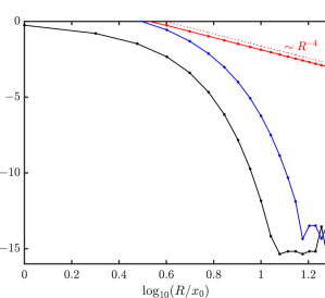
Figure 1: Plot of the relative error in the DDI energy computed using the bare interaction kernel Eq. (10) (red) and the cutoff kernel in Eq. (12) (blue) using $\psi_{\mathrm{tr}}$ with $l_{x}=\sqrt{2}x_{0}$ and $l_{y}=x_{0}/\sqrt{2}$. The black line shows the relative error in the integration of the density. The grid point density has been fixed to four per unit length.

In Fig. 1 we compare the error in calculating the DDI energy with and without a cutoff potential. This shows that in the absence of a cutoff there is a slow decay of the relative error in the energy of the DDI as the size of the grid is increased which demonstrates the inaccuracy that can arise due to improper treatment of the DDI. The relative error decays algebraically $\sim R^{-4}$ when there is no cutoff potential. However, once a cutoff is introduced, the error in this calculation falls off rapidly, converging to machine precision once the state is well represented on the grid.

The singular nature of the DDI potential has limited the development of analytic truncated kernels to two particular cases (see [33]), and our result developed here represents a new contribution. For other specific geometries the truncated kernels can be obtained numerically [34, 35], but these are not suitable for the tube situation we consider here. In our algorithm the numerical grid frequently changes (from the $L$ optimisation). This requires constant recomputing of the truncated kernel, making the analytical expression especially well-suited to our problem.

II.5 Characterising the ground states

To quantify the translational symmetry that is broken due to density modulation along $z$, we define the density contrast

$$\mathcal{C}=\frac{n_{\mathrm{max}}-n_{\mathrm{min}}}{n_{\mathrm{max}}+n_{\mathrm{min}}},$$ (20)

where $n_{\mathrm{max}}$ and $n_{\mathrm{min}}$ are the maximum and minimum of the density $|\psi|^{2}$ on the $z$-axis. For a uniform state, $\mathcal{C}=0$, and for a crystalline state $\mathcal{C}>0$. For $\mathcal{C}=1$ the density goes to zero on the $z$ axis.

Second, we are interested in quantifying the superfluid fraction of the system. Superfluidity of a Bose-Einstein condensate is associated with a broken global $U(1)$ symmetry. Notably, as pointed out by Leggett [36] if the translational invariance of the Hamiltonian is broken by the ground state, then the $T=0$ superfluid faction of a Bose gas can be reduced from unity. Thus as the we expect a reduction in the superfluid as the condensate develops crystalline structure. We can most directly quantify the superfluid fraction by computing the nonclassical translational inertia (see [37, 36, 38]) as

$$f_{s}=1-\lim_{v_{z}\to 0}\frac{\langle P_{z}\rangle}{nLmv_{z}},$$ (21)

where $\langle P_{z}\rangle=-i\hbar\int_{\mathrm{uc}}d\mathbf{x}\,\psi^{*}\frac{\partial}{\partial z}\psi$ is the expectation of the $z$-component of momentum in a frame moving with uniform velocity $v_{z}$. In Refs. [6, 36] Leggett developed bounds for the superfluid fraction such that $f_{s}^{l}\leq f_{s}\leq f_{s}^{u}$, where

$$f_{s}^{u}\equiv\frac{L}{n}\left[\int_{\mathrm{uc}}\frac{dz}{\int d\bm{\rho}\,|\psi|^{2}}\right]^{-1},$$ (22)

and,

$$f_{s}^{l}\equiv\frac{L}{n}\int d\bm{\rho}\,\left[\int_{\mathrm{uc}}\frac{dz}{|\psi|^{2}}\right]^{-1},$$ (23)

are the upper and lower bounds, respectively. These expressions can be directly computed from the ground state solution avoiding the need for additional calculations in a moving frame. While the measures in Eq. (22) and Eq. (23) are bounds of the superfluid fraction, for the infinite tube dipolar gas we have confirmed that $f_{s}$, $f_{s}^{u}$ and, $f_{s}^{l}$ are all in good agreement. Notably, for the results in Fig. 2 the maximum difference from the bounds to $f_{s}$ is $\sim 0.7\%$. The moving frame measure is more difficult to apply near the transition and for this reason the superfluid fraction results we present here are evaluated using Eq. (22).

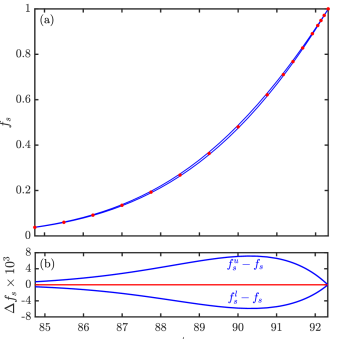
Figure 2: (a) Example of the superfluid fraction calculated by nonclassical translational inertia [Eq. (21)] (red dots), and the upper and lower bounds (blue lines) given by Eqs. (22) and (23), respectively. The difference between the results is barely visible. (b) The differences $f_{s}^{u}-f_{s}$ and $f_{s}^{l}-f_{s}$ (blue lines). Other parameters: ¹⁶⁴Dy Bose gas with $n=2500/\mu$m and $\omega_{x,y}/2\pi=150\,$Hz.

II.6 Reduced 3D theory

The reduced 3D theory was introduced in Ref. [26], and we briefly review it here as it is used to compare against the full 3D results for the phase diagram. The basis of this theory is to decompose the 3D field as $\psi(\mathbf{x})=\phi(z)\chi_{\mathrm{var}}(\bm{\rho})$ where $\chi_{\mathrm{var}}(\bm{\rho})=\tfrac{1}{\sqrt{\pi}l}{e^{-(\eta x^{2}+y^{2}/\eta)/2l^{2}}}$ is a two-dimensional Gaussian function with variational parameters $\{l,\eta\}$, and $\phi(z)$ describes the axial field with $\int_{\mathrm{uc}}dz\,|\phi|^{2}=nL$ and periodic boundary conditions. The energy per particle of the reduced theory is given by

$$\mathcal{E}_{\mathrm{red}}=\mathcal{E}_{\perp}+\int_{\mathrm{uc}}\!\frac{dz}{nL}\,\phi^{*}\!\left(\!-\frac{\hbar^{2}}{2m}\frac{d^{2}}{dz^{2}}+\frac{1}{2}\Phi+\frac{4\gamma_{\mathrm{QF}}|\phi|^{3}}{25\pi^{3/2}l^{3}}\right)\!\phi,$$ (24)

where

$$\mathcal{E}_{\perp}=\frac{\hbar^{2}}{4ml^{2}}\left(\eta+\frac{1}{\eta}\right)+\frac{ml^{2}}{4}\left(\frac{\omega_{x}^{2}}{\eta}+\omega_{y}^{2}\eta\right),$$ (25)

is the single-particle energy of the transverse degrees of freedom. The two-body interactions are described by the effective potential

$$\Phi(z)=\mathcal{F}_{z}^{-1}\left\{\tilde{U}(k_{z})\mathcal{F}_{z}\{|\phi|^{2}\}\right\},$$ (26)

with $\mathcal{F}_{z}$ being the 1D Fourier transform, and where

$$\tilde{U}(k_{z}) =\frac{g_{s}}{2\pi l^{2}}+\frac{g_{\mathrm{dd}}}{2\pi l^{2}}\!\left\{\!\frac{3[Qe^{Q}\operatorname{Ei}(-Q)+1]}{1+\eta}-1\!\right\},$$ (27)

with $\operatorname{Ei}$ being the exponential integral, and $Q\equiv\tfrac{1}{2}\sqrt{\eta}k_{z}^{2}l^{2}$ (see [27]). To obtain stationary solutions of the reduced theory we vary $\{l,\eta,L\}$ and $\psi(z)$ to find local minima of (24). This theory is rather efficient to solve and was used to construct a phase diagram for the infinite tube dipolar gas in Ref. [26].

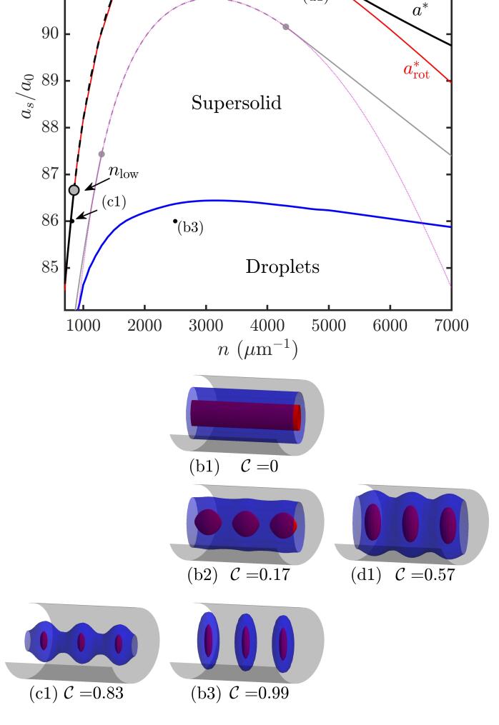
Figure 3: (a) Phase diagram for a ¹⁶⁴Dy Bose gas confined by a radially symmetric infinite tube trap with $\omega_{x,y}/2\pi=150\,$Hz. The black line indicates the crystallization transition boundary $a^{*}$. This line is solid where the transition is discontinuous and is dashed where it is continuous. The circles demarcate the start and the end of the continuous region at $n_{\mathrm{low}}$ and $n_{\mathrm{high}}$, respectively. The parameters where a roton excitation in the uniform state softens to zero energy are shown with the red line. The crystallization transition boundary of the reduced 3D theory is shown in grey, and the roton boundary from that theory in magenta. (b1)-(b3),(c1)-(d1) Example ground states for parameters indicated in subplot (a). Isodensity surfaces of $|\psi|^{2}$ (repeated over 3 unit cells for the modulated cases) taken at $75\%$ (red) and $1\%$ (blue) of the peak density. The grey isosurface indicates a cutaway isoenergy surface of the trapping potential.

III Results

III.1 Phase diagram

The results presented here are for a Bose gas of ¹⁶⁴Dy atoms with $a_{\mathrm{dd}}=130.8a_{0}$, confined to a radially symmetric trap with $\omega_{x,y}/2\pi=150\,$Hz. This system is similar to that considered for the main results of Ref. [26] calculated using the reduced theory. Figure 3(a) is the phase diagram obtained by minimising the energy per particle (5) as $a_{s}$ and $n$ are varied, and is the main result of this paper. We identify three different phases using the ground state properties. (i) The uniform Bose-Einstein condensate (BEC) is translationally invariant along $z$, with $\mathcal{C}=0$ and $f_{s}=1$ [see Fig. 3(b1)]; (ii) The supersolid state is a crystalline state with $\mathcal{C}>0$, yet retaining a finite superfluid fraction $f_{s}$ [see Figs. 3(b2), (c1), and (d1)]; (iii) The insulating droplet state is a crystalline state with tightly-bound and separated droplets [see Fig. 3(b3)]. For the insulating droplet state the contrast of the density modulation along $z$ is essentially complete ($\mathcal{C}\approx 1$) and the superfluid fraction is negligible $f_{s}\approx 0$. We do not concern ourselves with the nature of the transition or crossover from supersolid to insulating droplets. A proper description of this is beyond the eGPE theory, and requires a theory capable of capturing correlations between droplets needed to drive the insulating transition.

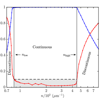
Figure 4: Superfluid fraction (blue) and density contrast (red) as a function of the average linear density of the crystalline state along the transition boundary $a^{*}$ [see Fig. 3]. The vertical lines identify the low density ($n_{\mathrm{low}}$) and high-density ($n_{\mathrm{high}}$) end points of the region in which the transition is continuous. The grey-shaded region indicates contrast values which we take to be zero (see text). Other parameters as in Fig. 3.

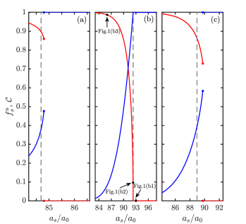
Figure 5: Behavior of the ground state density contrast (red) and superfluid fraction (blue) as $a_{s}$ varies across the transition for three different cases: (a) $n=710/\mu$m, (b) $n=2500/\mu$m, and (c) $n=7000/\mu$m. The vertical grey dashed lines indicate $a_{\mathrm{rot}}^{*}$ for each case. Other parameters as in Fig. 3.

We define $a^{*}$ as the value of $a_{s}$ at which the ground state transitions from a uniform BEC to having crystalline order (i.e. $\mathcal{C}=0$ to $\mathcal{C}\neq 0$) for a system with average linear density $n$. Over the range of $n$ values shown in Fig. 3(a) the transition occurs directly from the uniform BEC state into a supersolid state, with the insulating droplet state emerging at lower values of $a_{s}$. We observe that $a^{*}$ initially increases with $n$ as the role of interactions increases relative to kinetic energy, but then $a^{*}$ decreases for $n\gtrsim 2.8\times 10^{3}/\mu$m, as quantum fluctuation effects become stronger. Our main interest here is the nature of the BEC to crystalline transition. At each density $n$ we have obtained the crystalline ground state solution at the transition point $a^{*}$, where it is degenerate with the uniform BEC state. The contrast and superfluid fraction of these states are shown in Fig. 4, revealing that for an intermediate density range $n\in[n_{\mathrm{low}},n_{\mathrm{high}}]$ with $n_{\mathrm{low}}\approx 0.8\times 10^{3}/\mu$m and $n_{\mathrm{high}}\approx 4.5\times 10^{3}/\mu$m, the transition is continuous. That is, in this range $\mathcal{C}\to 0$ and $f_{s}\to 1$ as $a_{s}\to a^{*}$ from below. The end points of this continuous transition line are indicated by two circles in Fig. 3(a).

In Fig. 5 we examine the variation of the superfluid fraction and the density contrast of the ground state as a function of $a_{s}$. We present a low density discontinuous case [Fig. 5(a)], an intermediate density continuous case [Fig. 5(b)], and a high density discontinuous case [Fig. 5(c)]. These results also show that in the discontinuous transition the superfluid fraction of the crystalline state is significantly less than unity, even for $a_{s}$ values very close to the transition. In contrast, in the vicinity of the continuous transition the superfluid fraction of the crystalline state tends to be close to unity for an appreciable range of $a_{s}$ values below $a^{*}$.

Since crystalline order causes a reduction in the superfluid fraction we can use either $f_{s}$ or $\mathcal{C}$ to quantify the crystalline transition (e.g. cf. Refs. [25, 26, 39]). The density contrast $\mathcal{C}$ is most frequently used in application to the experimental regime with a cigar shaped harmonic trap. Our results show that immediately below the continuous transition point $\mathcal{C}$ charges more rapidly with $a_{s}$ than $f_{s}$ [see Fig. 5(b)]. This can be understood by a simplified analytic model of the weakly modulated state developed in Ref. [26], which shows that in the vicinity of the continuous transition for small $\mathcal{C}$, the reduction in superfluid fraction is second order in $\mathcal{C}$ [40]

$$f_{s}=1-\frac{1}{2}\mathcal{C}^{2}+O(\mathcal{C}^{4}).$$ (28)

If the transition is continuous or almost continuous then, near the transition, (weakly) crystalline and uniform states have very similar energy, which makes precisely determining $a^{*}$ challenging. For the results presented in Fig. 4, we have taken cases with $\mathcal{C}<0.1$ to be equivalent to $\mathcal{C}=0$ (i.e. results in the grey shaded region), and identified these as being the continuous transition regime. We find $a^{*}$ to an accuracy of $\sim 10^{-4}\,a_{0}$, which requires resolving a difference in the relative energy per particle of crystalline and uniform states to $\sim 10^{-7}$. In contrast, the difference in the numerically obtained $f_{s}$ from unity at $a^{*}$ is almost too small to notice in Fig. 4, i.e. the scatter in $f_{s}$ is less than 1% [consistent with Eq. (28)].

For comparison, we also indicate the phase transition from the reduced theory in Fig. 3(a). The transition boundary $a^{*}$ predicted by the reduced theory is approximately $1\,a_{0}$ to $2\,a_{0}$ lower than that of the full eGPE calculation. This shift arises from the variational treatment of the transverse degrees of freedom in the reduced theory, and is consistent with other such comparisons of the reduced theory to full 3D calculations (e.g. see the shifts in scattering lengths for the occurrence of rotons noted in Fig. 5 of [27]).

III.2 Roton softening and the continuous transition

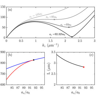
Figure 6: (a) Dispersion relation of the lowest Bogoliubov excitation band for a uniform BEC state for $a_{s}$ values as indicated. A roton excitation manifests as a local minimum in this dispersion relation (marked with $\times$). The roton softens to zero energy as $a_{s}\to a_{\mathrm{rot}}^{*}$ from above. (b) Energy per particle of the uniform (blue line) and modulated (red line) states; the black dot indicates where the energies cross. (c) Length $L$ of the uc (undefined out of the crystalline phase). The red dot has coordinates $(a_{\mathrm{rot}}^{*},\lambda_{\mathrm{rot}}$) where $\lambda_{\mathrm{rot}}=2\pi/k_{\mathrm{rot}}$ is the roton wavelength and $k_{\mathrm{rot}}>0$ is the wavevector where the dispersion touches zero. Results for $n=2500/\mu$m and other parameters as in Fig. 3.

We determined the collective excitations of the uniform BEC state by solving the Bogoliubov-de Gennes equations (see Ref. [27] for details). As the uniform groundstate is translationally invariant, the excitations can be characterized by the $z$-component of momentum ($\hbar k_{z}$), and occur as a set of bands with different transverse excitation. In Fig. 6(a) we show the results for the lowest excitation band for a system with $n=2500/\mu$m and at various $a_{s}$ values. At the highest value shown ($a_{s}=105a_{0}$) the spectrum is a monotonically increasing function of $k_{z}$. As $a_{s}$ is lowered, a local minimum develops at a non-zero wavevector, a roton-like mode which arises in dipolar BECs from the interplay of the DDIs and confinement [41, 42, 43]. The minimum energy of the roton decreases with decreasing $a_{s}$, until the energy softens to zero energy. We identify the value of scattering length when this occurs as $a_{\mathrm{rot}}^{*}$, and the corresponding $k_{z}$ value of the zero-energy mode as the roton wavevector $k_{\mathrm{rot}}$. For $a_{s}<a_{\mathrm{rot}}^{*}$ the roton is dynamically unstable, indicating that the uniform BEC state is no longer the ground state [see Fig. 6(b)]. For the density considered in these results $a_{\mathrm{rot}}^{*}=a^{*}$ [cf. Fig. 5(b)] and the roton softening marks the critical point at which the crystalline order continuously emerges. In Fig. 6(c) we show that the uc length $L$ of the crystalline ground state corresponds to the roton wavelength at the critical point.

We indicate the roton instability as a function of density in the phase diagram, Fig. 3(a). We see that where a continuous transition is found, the roton instability coincides with the transition, i.e. $a^{*}=a_{\mathrm{rot}}^{*}$ for $n\in[n_{\mathrm{low}},n_{\mathrm{high}}]$. Outside of this region $a_{\mathrm{rot}}^{*}<a^{*}$, such that the uniform BEC state is energetically unstable for $a_{s}<a^{*}$, but not dynamically unstable until $a_{s}<a_{\mathrm{rot}}^{*}$.

Ref. [25] considers a finite tube with periodic boundary conditions and a fixed unit cell size, and finds a discontinuous $\sim 10\%$ jump in $f_{s}$ at the crystallization transition. We have performed calculations for those parameters (¹⁶⁶Er Bose gas with $n=3.78\times 10^{3}/\mu$m and $\omega_{x,y}/2\pi=600\,$Hz), but for an infinite tube with the unit cell size chosen to minimize energy. We find that the transition to the crystalline transition is continuous and occurs with $a^{*}=a_{\mathrm{rot}}^{*}$ [similar to Fig. 6(a) and 5(b)]. The fixed system length (e.g., not being an integer multiple of $\lambda_{\mathrm{rot}}$) and the absence of a truncated DDI potential for the calculations in Ref. [25] may have contributed to the prediction of a discontinuous transition.

III.3 Discontinuous phase transition

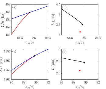
Figure 7: (a,c) Energy per particle of modulated state (red) and uniform state (blue); the black dot indicates where the energies cross. (b,d) Length of the uc for the crystalline state. The red dot has coordinates $(a_{\mathrm{rot}}^{*},\lambda_{\mathrm{rot}}$). (a,b) $n=710/\mu$m and (c,d) $n=7000/\mu$m, with other parameters as in Fig. 3.

In Fig. 7 we examine the behavior of the transition for low- and high-density discontinuous cases. Here the energy per particle of the uniform and crystalline states cross [difficult to see in Figs. 7 (a) and (c)]. We are unable to follow the crystalline branch to values of $a_{s}$ much higher than $a^{*}$ because the gradient flow algorithm is an energy minimisation scheme and causes the crystalline state to jump to the uniform branch. In contrast, we are able to solve for the uniform solution for $a_{s}<a^{*}$ using the ansatz $\psi=\sqrt{n}\chi(\bm{\rho})$, which does not allow any modulation to develop along $z$. The uc length comparison in Figs. 7(a) and (c) also shows that the crystalline states have $L>\lambda_{\mathrm{rot}}$ in the region of the discontinuous transition. The high density discontinuous transition occurs in a regime where the quantum fluctuation effects are relatively strong and has been identified as a fluctuation induced first order transition in the finite system studied in Ref. [39].

IV Conclusions

In this paper we have developed and applied a numerical method to study the ground states of a dipolar Bose gas in an infinite tube potential. We perform these calculations within an optimized unit cell, utilizing an analytic result for a truncated DDI kernel. Using our method, we have explored the BEC to crystalline transition as a function of the average linear density for a system with isotropic transverse trapping. We find that a continuous transition to the crystalline state occurs for intermediate densities, and that in the vicinity of the continuous transition, the crystalline state has a significant superfluid fraction, and thus may be a useful regime to study supersolidity. These results demonstrate that the reduced 3D theory developed in Ref. [26] provides a qualitatively accurate description of the transitions in this system, however the transition lines of the reduced 3D theory are shifted to lower values of $a_{s}$. Our results verify that the continuous transition occurs coincident with the softening of a roton excitation in the uniform BEC state, which initiates the crystallization at the roton wavelength. For densities where the transition is discontinuous, the roton softens at a value of $a_{s}$ below $a^{*}$. This behavior may allow hysteresis to occur such that, as $a_{s}$ is ramped across the transition, the BEC could persist to values of $a_{s}$ below $a^{*}$. Similarly, the crystalline state could persist to values of $a_{s}$ above $a^{*}$.

In future work we will study the behavior of the transition in the low density regime in more detail. It is of interest to understand if the transition to the crystalline state in this regime occurs directly into a well-separated insulating droplet state or some other arrangement. Another issue is to understand the role of the transverse confinement, especially when it is anisotropic. A deeper understanding of these effects will provide insight into the nature of the transition in the finite system (e.g. 3D cigar trap, see [39, 44]), and will provide a point of comparison to work looking at crystallization and supersolids in 2D (e.g. see [45, 46, 47, 48, 49, 50, 51, 52, 51]).

References

- Gross [1957] E. P. Gross, Unified theory of interacting bosons, Phys. Rev. 106, 161 (1957).
- Penrose and Onsager [1956] O. Penrose and L. Onsager, Bose-Einstein condensation and liquid helium, Phys. Rev. 104, 576 (1956).
- Andreev and Lifshitz [1969] A. Andreev and I. Lifshitz, Quantum theory of defects in crystals, JETP 29, 1107 (1969).
- Chester [1970] G. V. Chester, Speculations on Bose-Einstein condensation and quantum crystals, Phys. Rev. A 2, 256 (1970).
- Gross [1958] E. Gross, Classical theory of boson wave fields, Ann. Phys. 4, 57 (1958).
- Leggett [1970] A. J. Leggett, Can a solid be "superfluid"?, Phys. Rev. Lett. 25, 1543 (1970).
- Greywall [1977] D. S. Greywall, Search for superfluidity in solid , Phys. Rev. B 16, 1291 (1977).
- Kim and Chan [2004a] E. Kim and M. H. W. Chan, Probable observation of a supersolid helium phase, Nature 427, 225 (2004a).
- Kim and Chan [2004b] E. Kim and M. H. W. Chan, Observation of superflow in solid helium, Science 305, 1941 (2004b).
- Kim and Chan [2012] D. Y. Kim and M. H. W. Chan, Absence of supersolidity in solid helium in porous vycor glass, Phys. Rev. Lett. 109, 155301 (2012).
- Boninsegni and Prokof’ev [2012] M. Boninsegni and N. V. Prokof’ev, Colloquium: Supersolids: What and where are they?, Rev. Mod. Phys. 84, 759 (2012).
- Léonard et al. [2017] J. Léonard, A. Morales, P. Zupancic, T. Esslinger, and T. Donner, Supersolid formation in a quantum gas breaking a continuous translational symmetry, Nature 543, 87 (2017).
- Li et al. [2017] J.-R. Li, J. Lee, W. Huang, S. Burchesky, B. Shteynas, F. Ç. Top, A. O. Jamison, and W. Ketterle, A stripe phase with supersolid properties in spin–orbit-coupled Bose–Einstein condensates, Nature 543, 91 (2017).
- Chomaz et al. [2019] L. Chomaz, D. Petter, P. Ilzhöfer, G. Natale, A. Trautmann, C. Politi, G. Durastante, R. M. W. van Bijnen, A. Patscheider, M. Sohmen, M. J. Mark, and F. Ferlaino, Long-lived and transient supersolid behaviors in dipolar quantum gases, Phys. Rev. X 9, 021012 (2019).
- Böttcher et al. [2019] F. Böttcher, J.-N. Schmidt, M. Wenzel, J. Hertkorn, M. Guo, T. Langen, and T. Pfau, Transient supersolid properties in an array of dipolar quantum droplets, Phys. Rev. X 9, 011051 (2019).
- Tanzi et al. [2019a] L. Tanzi, E. Lucioni, F. Famà, J. Catani, A. Fioretti, C. Gabbanini, R. N. Bisset, L. Santos, and G. Modugno, Observation of a dipolar quantum gas with metastable supersolid properties, Phys. Rev. Lett. 122, 130405 (2019a).
- Tanzi et al. [2019b] L. Tanzi, S. M. Roccuzzo, E. Lucioni, F. Famà, A. Fioretti, C. Gabbanini, G. Modugno, A. Recati, and S. Stringari, Supersolid symmetry breaking from compressional oscillations in a dipolar quantum gas, Nature 574, 382 (2019b).
- Guo et al. [2019] M. Guo, F. Böttcher, J. Hertkorn, J.-N. Schmidt, M. Wenzel, H. P. Büchler, T. Langen, and T. Pfau, The low-energy Goldstone mode in a trapped dipolar supersolid, Nature 564, 386 (2019).
- Natale et al. [2019] G. Natale, R. M. W. van Bijnen, A. Patscheider, D. Petter, M. J. Mark, L. Chomaz, and F. Ferlaino, Excitation spectrum of a trapped dipolar supersolid and its experimental evidence, Phys. Rev. Lett. 123, 050402 (2019).
- Ferrier-Barbut et al. [2016] I. Ferrier-Barbut, H. Kadau, M. Schmitt, M. Wenzel, and T. Pfau, Observation of quantum droplets in a strongly dipolar Bose gas, Phys. Rev. Lett. 116, 215301 (2016).
- Wächtler and Santos [2016] F. Wächtler and L. Santos, Quantum filaments in dipolar Bose-Einstein condensates, Phys. Rev. A 93, 061603(R) (2016).
- Bisset et al. [2016] R. N. Bisset, R. M. Wilson, D. Baillie, and P. B. Blakie, Ground-state phase diagram of a dipolar condensate with quantum fluctuations, Phys. Rev. A 94, 033619 (2016).
- Lee and Yang [1957] T. D. Lee and C. N. Yang, Many-body problem in quantum mechanics and quantum statistical mechanics, Phys. Rev. 105, 1119 (1957).
- Lima and Pelster [2012] A. R. P. Lima and A. Pelster, Beyond mean-field low-lying excitations of dipolar Bose gases, Phys. Rev. A 86, 063609 (2012).
- Roccuzzo and Ancilotto [2019] S. M. Roccuzzo and F. Ancilotto, Supersolid behavior of a dipolar Bose-Einstein condensate confined in a tube, Phys. Rev. A 99, 041601(R) (2019).
- Blakie et al. [2020a] P. B. Blakie, D. Baillie, L. Chomaz, and F. Ferlaino, Supersolidity in an elongated dipolar condensate, Phys. Rev. Research 2, 043318 (2020a).
- Blakie et al. [2020b] P. B. Blakie, D. Baillie, and S. Pal, Variational theory for the ground state and collective excitations of an elongated dipolar condensate, Commun. Theor. Phys. 72, 085501 (2020b).
- Lima and Pelster [2011] A. R. P. Lima and A. Pelster, Quantum fluctuations in dipolar Bose gases, Phys. Rev. A 84, 041604(R) (2011).
- Lee et al. [2021] A.-C. Lee, D. Baillie, and P. B. Blakie, Numerical calculation of dipolar-quantum-droplet stationary states, Phys. Rev. Research 3, 013283 (2021).
- Bao et al. [2010] W. Bao, Y. Cai, and H. Wang, Efficient numerical methods for computing ground states and dynamics of dipolar Bose–Einstein condensates, J. Comput. Phys. 229, 7874 (2010).
- Kelley [2003] C. T. Kelley, Solving nonlinear equations with Newton’s method (SIAM, 2003).
- Gradshteyn and Ryzhik [2007] I. S. Gradshteyn and I. M. Ryzhik, Table of integrals, series, and products, 7th ed. (Academic Press, San Diego, 2007).
- Ronen et al. [2006] S. Ronen, D. C. E. Bortolotti, and J. L. Bohn, Bogoliubov modes of a dipolar condensate in a cylindrical trap, Phys. Rev. A 74, 013623 (2006).
- Lu et al. [2010] H.-Y. Lu, H. Lu, J.-N. Zhang, R.-Z. Qiu, H. Pu, and S. Yi, Spatial density oscillations in trapped dipolar condensates, Phys. Rev. A 82, 023622 (2010).
- Tang et al. [2017] Q. Tang, Y. Zhang, and N. J. Mauser, A robust and efficient numerical method to compute the dynamics of the rotating two-component dipolar Bose–Einstein condensates, Comput. Phys. Commun. 219, 223 (2017).
- Leggett [1998] A. J. Leggett, On the superfluid fraction of an arbitrary many-body system at , J. Stat. Phys. 93, 927 (1998).
- Pomeau and Rica [1994] Y. Pomeau and S. Rica, Dynamics of a model of supersolid, Phys. Rev. Lett. 72, 2426 (1994).
- Sepúlveda et al. [2008] N. Sepúlveda, C. Josserand, and S. Rica, Nonclassical rotational inertia fraction in a one-dimensional model of a supersolid, Phys. Rev. B 77, 054513 (2008).
- Biagioni et al. [2022] G. Biagioni, N. Antolini, A. Alaña, M. Modugno, A. Fioretti, C. Gabbanini, L. Tanzi, and G. Modugno, Dimensional crossover in the superfluid-supersolid quantum phase transition, Phys. Rev. X 12, 021019 (2022).
- Chomaz [2020] L. Chomaz, Probing the supersolid order via high-energy scattering: Analytical relations among the response, density modulation, and superfluid fraction, Phys. Rev. A 102, 023333 (2020).
- Santos et al. [2003] L. Santos, G. V. Shlyapnikov, and M. Lewenstein, Roton-maxon spectrum and stability of trapped dipolar Bose-Einstein condensates, Phys. Rev. Lett. 90, 250403 (2003).
- Chomaz et al. [2018] L. Chomaz, R. M. W. van Bijnen, D. Petter, G. Faraoni, S. Baier, J. H. Becher, M. J. Mark, F. Wächtler, L. Santos, and F. Ferlaino, Observation of roton mode population in a dipolar quantum gas, Nat. Phys. 14, 442 (2018).
- Petter et al. [2019] D. Petter, G. Natale, R. M. W. van Bijnen, A. Patscheider, M. J. Mark, L. Chomaz, and F. Ferlaino, Probing the roton excitation spectrum of a stable dipolar Bose gas, Phys. Rev. Lett. 122, 183401 (2019).
- Alaña et al. [2022] A. Alaña, N. Antolini, G. Biagioni, I. L. Egusquiza, and M. Modugno, Crossing the superfluid-supersolid transition of an elongated dipolar condensate, Phys. Rev. A 106, 043313 (2022).
- Lu et al. [2015] Z.-K. Lu, Y. Li, D. S. Petrov, and G. V. Shlyapnikov, Stable dilute supersolid of two-dimensional dipolar bosons, Phys. Rev. Lett. 115, 075303 (2015).
- Zhang et al. [2019] Y.-C. Zhang, F. Maucher, and T. Pohl, Supersolidity around a critical point in dipolar Bose-Einstein condensates, Phys. Rev. Lett. 123, 015301 (2019).
- Baillie and Blakie [2018] D. Baillie and P. B. Blakie, Droplet crystal ground states of a dipolar Bose gas, Phys. Rev. Lett. 121, 195301 (2018).
- Zhang et al. [2021] Y.-C. Zhang, T. Pohl, and F. Maucher, Phases of supersolids in confined dipolar Bose-Einstein condensates, Phys. Rev. A 104, 013310 (2021).
- Norcia et al. [2021] M. A. Norcia, C. Politi, L. Klaus, E. Poli, M. Sohmen, M. J. Mark, R. N. Bisset, L. Santos, and F. Ferlaino, Two-dimensional supersolidity in a dipolar quantum gas, Nature 596, 357 (2021).
- Schmidt et al. [2021] J.-N. Schmidt, J. Hertkorn, M. Guo, F. Böttcher, M. Schmidt, K. S. H. Ng, S. D. Graham, T. Langen, M. Zwierlein, and T. Pfau, Roton excitations in an oblate dipolar quantum gas, Phys. Rev. Lett. 126, 193002 (2021).
- Hertkorn et al. [2021] J. Hertkorn, J.-N. Schmidt, M. Guo, F. Böttcher, K. S. H. Ng, S. D. Graham, P. Uerlings, H. P. Büchler, T. Langen, M. Zwierlein, and T. Pfau, Supersolidity in two-dimensional trapped dipolar droplet arrays, Phys. Rev. Lett. 127, 155301 (2021).
- Poli et al. [2021] E. Poli, T. Bland, C. Politi, L. Klaus, M. A. Norcia, F. Ferlaino, R. N. Bisset, and L. Santos, Maintaining supersolidity in one and two dimensions, Phys. Rev. A 104, 063307 (2021).