An efficient symmetric primal-dual algorithmic framework for saddle point problems

Abstract

In this paper, we propose a new primal-dual algorithmic framework for a class of convex-concave saddle point problems frequently arising from image processing and machine learning. Our algorithmic framework updates the primal variable between the twice calculations of the dual variable, thereby appearing a symmetric iterative scheme, which is accordingly called the symmetric primal-dual algorithm (SPIDA). It is noteworthy that the subproblems of our SPIDA are equipped with Bregman proximal regularization terms, which make SPIDA versatile in the sense that it enjoys an algorithmic framework covering some existing algorithms such as the classical augmented Lagrangian method (ALM), linearized ALM, and Jacobian splitting algorithms for linearly constrained optimization problems. Besides, our algorithmic framework allows us to derive some customized versions so that SPIDA works as efficiently as possible for structured optimization problems. Theoretically, under some mild conditions, we prove the global convergence of SPIDA and estimate the linear convergence rate under a generalized error bound condition defined by Bregman distance. Finally, a series of numerical experiments on the matrix game, basis pursuit, robust principal component analysis, and image restoration demonstrate that our SPIDA works well on synthetic and real-world datasets.

1 Introduction

Recently, saddle point problems have received much considerable attention in the signal/image processing, machine learning, and optimization communities, e.g., see [10, 11, 18, 49, 59], to name just a few. In this paper, we are interested in the convex-concave saddle point problem with a bilinear coupling term, which takes the following form:

(1) $$\min_{x\in{\mathcal{X}}}\max_{y\in{\mathcal{Y}}}\left\{{\mathscr{L}}(x,y):=f(x)+\langle Ax,y\rangle-g(y)\right\},$$

where ${\mathcal{X}}\subseteq{\mathbb{R}}^{n}$ and ${\mathcal{Y}}\subseteq{\mathbb{R}}^{m}$ are two closed nonempty convex sets, both $f(\cdot):{\mathcal{X}}\rightarrow(-\infty,\infty]$ and $g(\cdot):{\mathcal{Y}}\rightarrow(-\infty,\infty]$ are proper closed convex (possibly nonsmooth) functions, $\langle\cdot,\cdot\rangle$ represents the standard inner product of vectors, and $A:{\mathbb{R}}^{n}\rightarrow{\mathbb{R}}^{m}$ is a bounded linear operator. It is interesting that (1) provides a unified framework for the treatment of convex composite optimization problem

(2) $$\min_{x\in{\mathbb{R}}^{n}}\left\{f(x)+g^{*}(Ax)\right\}$$

and the canonical convex minimization problem with linear constraints (see Section 4), where $g^{*}(\cdot)$ is the Fenchel conjugate of the function $g(\cdot)$. Here, we refer the reader to [38, 49, 52] for surveys on this topic.

To efficiently exploit the min-max structure of (1), a seminal work can be traced back to the Arrow-Hurwicz Primal-Dual (AHPD) method [1], which updates the primal and dual variables in a sequential order by solving two optimization subproblems as follows:

(3) $$\left\{\begin{aligned} x^{k+1}&=\arg\min_{x\in\mathcal{X}}\left\{f(x)+\langle Ax,y^{k}\rangle+\frac{\mu}{2}\|x-x^{k}\|^{2}\right\},\\ y^{k+1}&=\arg\max_{y\in\mathcal{Y}}\left\{-g(y)+\langle Ax^{k+1},y\rangle-\frac{\gamma}{2}\|y-y^{k}\|^{2}\right\},\end{aligned}\right.$$

where $\mu$ and $\gamma$ are two positive proximal regularization parameters serving as step sizes for updating. In the literature, such a method is also reemphasized as primal-dual hybrid gradient (PDHG) method, which has been widely used in image processing [5, 18, 26, 59]. Although some convergence properties have been established under additional conditions [18, 29, 43], the most recent work [28] showed that the AHPD method with any constant step size is not necessarily convergent for solving generic convex-concave saddle point problems. In 2011, Chambolle and Pock [10] judiciously introduced a First-Order Primal-Dual Algorithm (FOPDA) by absorbing an extrapolation step for algorithmic acceleration. Specifically, for given the $k$-th iterate $(x^{k},y^{k})$, the iterative scheme of FOPDA reads as

$$x^{k+1}=\arg\min_{x\in\mathcal{X}}\left\{f(x)+\langle Ax,y^{k}\rangle+\frac{\mu}{2}\|x-x^{k}\|^{2}\right\},$$

(4) $$\tilde{x}^{k+1}=x^{k+1}+\tau(x^{k+1}-x^{k}),$$

$$y^{k+1}=\arg\max_{y\in\mathcal{Y}}\left\{-g(y)+\langle A\tilde{x}^{k+1},y\rangle-\frac{\gamma}{2}\|y-y^{k}\|^{2}\right\},$$

where $\tau\in[0,1]$ is an extrapolation parameter and both $\mu>0$ and $\gamma>0$ are regularization parameters. In particular, they further proved some promising convergence properties for the special case $\tau=1$ under the following requirement:

(5) $$\|AA^{\top}\|<\mu\gamma.$$

It is notable that the FOPDA not only requires weaker convergence-guaranteeing conditions, but also runs faster than the AHPD method (see [10, 12]). In recent years, there are some papers contributed to further studies on the extrapolation step, e.g., see [8, 13, 30, 32, 54]. As aforementioned, both $\mu$ and $\gamma$ serve as step sizes for updating. From computational perspective, larger step sizes usually lead to faster convergence, which accordingly encourages researchers to relax the condition (5), e.g., see [25, 37, 39, 40]. When the $x$- and $y$-subproblems are not easily to be solved or the maximum eigenvalue of $AA^{\top}$ cannot be easily evaluated in some cases, the better ways are solving the underlying subproblems in an inexact way and applying line search to avoid the calculation of $\|AA^{\top}\|$, e.g., see [14, 35, 36, 41, 48].

It is well-known that the saddle point problem (1) provides a powerful treatment for linearly constrained convex optimization problems (e.g., see Section 4). In this application, the dual variable $y$ in (1) serves as the so-called Lagrangian multiplier. However, as shown in the excellent overview on a phenomenon of slow convergence of optimization algorithms [34] (also see some comments [19, 42, 44, 50]), critical multipliers are nonempty for optimal solutions with nonunique Lagrangian multipliers, which play a crucial negative role in numerical optimization yielding slow convergence of major primal-dual algorithms, including Newton and Newton-related methods, the Augmented Lagrangian Method (ALM), and the sequential quadratic programming. Therefore, these surprising discoveries clearly demonstrate that the updating scheme of the dual variable (i.e., Lagrangian multiplier) is very important for algorithmic acceleration, which motivates us to develop some “dual stabilization techniques” for solving (1). Besides, most of saddle point problems arising from machine learning and image processing display unbalanced primal and dual subproblems in the sense that the dual problem is often easier than the primal one (e.g., see [10, 11] and also Section 4). As studied in the most recent work [31], balancing the subproblems of the classical ALM is able to greatly speed up the convergence of solving linearly constrained optimization problems. Therefore, how to balance both subproblems and what will be produced by some balancing technique for (1) are also motivations of this paper.

Considering the different complexity of primal and dual subproblems, we in this paper employ the symmetric spirit to design a new primal-dual algorithmic framework for saddle point problem (1), where the primal variable is updated once between the twice calculations of the dual variable. To a certain extent, our algorithm is able to balance the computation of primal and dual subproblems, and the one more calculation of the dual variable can be regarded as some dual stabilization technique from numerical perspective. Since the proposed algorithm appears a symmetric updating order on the dual variable, we call it symmetric primal-dual algorithm and denote it by SPIDA. A toy example shows that our SPIDA has a nice convergence behavior, while the AHPD fails to converge and the FOPDA runs a little slower than our SPIDA for some proximal parameters. Notice that each subproblem is equipped with a Bregman proximal term to make our algorithm versatile so that we can easily derive some classical first-order optimization methods, including the ALM and its linearized version for one-block linearly constrained convex optimization problems, and some Jacobian splitting algorithms for multi-block linearly constrained convex minimization problems. Particularly, our algorithmic framework is of benefit for producing some customized variants for linearly constrained optimization problems. Theoretically, we prove that our SPIDA is globally convergent under standard conditions, while the linear convergence rate is also estimated under a generalized error bound condition defined by Bregman distance. Finally, a series of numerical experiments on matrix games, basis pursuit, robust principal component analysis (RPCA), and image restoration demonstrate that our SPIDA performs better than some state-of-the-art primal-dual algorithms in many cases.

The remainder of paper is organized as follows. In Section 2, we recall some notations and definitions that will be used throughout this paper. In Section 3, we first describe the details of our proposed SPIDA for (1). Then, we prove its global convergence and estimate its linear convergence rate. In Section 4, we apply our SPIDA to solve the linearly constrained convex minimization problems, and show that some classical first-order optimization methods are special cases of the proposed SPIDA. In Section 5, we conduct the numerical performance of our SPIDA on solving some structured optimization problems with synthetic and real datasets. Finally, we complete this paper with drawing some conclusions in Section 6.

2 Preliminaries

In this section, we summarize some notations and basic concepts that will be used in subsequent analysis.

Throughout this paper, the superscript symbol ^⊤ represents the transpose for vectors and matrices. Let ${\mathbb{R}}^{n}$ be an $n$-dimensional Euclidean space endowed with the $M$-inner product $\langle x,y\rangle_{M}=\langle x,My\rangle=x^{\top}My$, where $x,y\in{\mathbb{R}}^{n}$ and $M$ is a symmetric and positive definite (or semi-definite) matrix ($M\succ 0$ (or $\succeq 0$) for short). Consequently, for a given vector $x\in{\mathbb{R}}^{n}$, we define the $M$-norm by

(6) $$\|x\|_{M}=\sqrt{\left\langle x,Mx\right\rangle}.$$

In particular, when $M$ is an identity matrix, the $M$-norm reduces to the standard Euclidean norm (denoted by $\|x\|$). Moreover, for a matrix $A$, we use $\|A\|$ to represent the square root of the maximum eigenvalue of $A^{\top}A$.

Definition 1.

Let $f(\cdot):{\mathbb{R}}^{n}\to(-\infty,+\infty]$ be an extended-real-valued function, and denote the domain of $f(\cdot)$ by $\mathrm{\bf dom}\,{(f)}:=\left\{x\in{\mathbb{R}}^{n}\;|\;f(x)<\infty\right\}$. Then, we say that the function $f(\cdot)$ is

1. proper if $f(x)>-\infty$ for all $x\in{\mathbb{R}}^{n}$ and $\mathrm{\bf dom}\,{(f)}\neq\emptyset$;

2. convex if $f\left(tx+(1-t)y\right)\leq tf(x)+(1-t)f(y)$ for every $x,y\in{\mathbb{R}}^{n}$ and $t\in[0,1]$;

3. $\varrho$-strongly convex with a given $\varrho>0$ if $\mathrm{\bf dom}\,{(f)}$ is convex and the following inequality holds for any $x,y\in\mathrm{\bf dom}\,{(f)}$ and $t\in[0,1]$:

   $$f(tx+(1-t)y)\leq tf(x)+(1-t)f(y)-\frac{\varrho}{2}t(1-t)\|x-y\|^{2}.$$

Let $f(\cdot):{\mathbb{R}}^{n}\to(-\infty,+\infty]$ be a proper, closed and convex function, then the subdifferential of $f(\cdot)$ at $x\in\mathrm{\bf dom}\,{(f)}$ is given by

$$\partial f(x)=\left\{\;\xi\,|\,f(z)\geq f(x)+\left\langle z-x,\xi\right\rangle,\,\forall\,z\in\mathrm{\bf dom}\,{(f)}\;\right\}.$$

In what follows, we denote $\mathrm{\bf dom}\,{(\partial f)}:=\{x\in{\mathbb{R}}^{n}\;|\;\partial f(x)\neq\emptyset\}$. Then, the following first-order characterizations of strong convexity are frequently used for analysis (e.g., see [3, Theorem 5.24]).

Lemma 2.

Let $f(\cdot):{\mathbb{R}}^{n}\to(-\infty,\infty]$ be a proper closed and convex function. Then, for a given $\varrho>0$, the following three claims are equivalent:

• $f(\cdot)$ is $\varrho$-strongly convex.

• $f(y)\geq f(x)+\langle\xi,y-x\rangle+\frac{\varrho}{2}\|y-x\|^{2}$ for any $x\in\mathrm{\bf dom}\,{(\partial f)}$, $y\in\mathrm{\bf dom}\,{(f)}$, and $\xi\in\partial f(x)$.

• $\langle\xi-\eta,x-y\rangle\geq\varrho\|x-y\|^{2}$ for any $x,y\in\mathrm{\bf dom}\,{(\partial f)}$ and $\xi\in\partial f(x)$, $\eta\in\partial f(y)$.

The proximal operator of $f$ (see [45, 47]), denoted by $\mathrm{\bf Prox}_{f}(\cdot)$, is given by

$$\mathrm{\bf Prox}_{f}(a)=\arg\min_{x\in{\mathbb{R}}^{n}}\left\{f(x)+\frac{1}{2}\|x-a\|^{2}\right\},\quad a\in{\mathbb{R}}^{n}.$$

Particularly, if $f(\cdot)$ is the indicator function $\delta_{\mathcal{X}}(\cdot)$ associated with the nonempty convex set ${\mathcal{X}}$, i.e.,

$$\delta_{\mathcal{X}}(x)=\left\{\begin{array}[]{ll}0,&\;\;\text{if}\;x\in{\mathcal{X}},\\ +\infty,&\;\;\text{otherwise},\end{array}\right.$$

then the proximal operator $\mathrm{\bf Prox}_{f}(\cdot)$ immediately reduces to the projection operator, i.e., $\mathrm{\bf Prox}_{f}(\cdot)\equiv\Pi_{\mathcal{X}}(\cdot)$. Let $\Omega$ be a nonempty closed convex set of ${\mathbb{R}}^{n}$, we define

$$\mathrm{\bf dist}_{M}(x,\Omega):=\min\;\left\{\|x-z\|_{M}\;|\;z\in\Omega\right\}$$

as the distance from any $x\in{\mathbb{R}}^{n}$ to the set $\Omega$ in the sense of matrix norm, where $M$ is a given symmetric and positive definite matrix. In particular, when $M$ is an identity matrix, we use $\mathrm{\bf dist}(x,\Omega)$ to denote the Euclidean distance from any $x$ to the set $\Omega$ for simplicity.

Given a proper closed strictly convex function $\phi(\cdot):{\mathbb{R}}^{n}\to(-\infty,+\infty]$, finite at $x$, $y$ and differentiable at $y$, the Bregman distance [7] between $x$ and $y$ associated with the kernel function $\phi$ is defined as

$$\mathscr{B}_{\phi}(x,y)=\phi(x)-\phi(y)-\langle\nabla\phi(y),x-y\rangle,$$

where $\nabla\phi(y)$ represents the gradient of $\phi$ at point $y$. It is not difficult to see that the Bregman distance covers the standard Euclidean distance as its special case when $\phi(\cdot)=\frac{1}{2}\|\cdot\|^{2}$. Here, we summarize three widely used Bregman distances in Table 1. However, the Bregman distance does not always share the symmetry and the triangle inequality property with the Euclidean distance.

Table 1: Three popular Bregman distances.

Type	Kernel function $\phi(\cdot)$	Bregman distance $\mathscr{B}_{\phi}(x,y)$
I	$\frac{1}{2}\|z\|^{2}$	$\frac{1}{2}\|x-y\|^{2}$,   $\forall x,y\in{\mathbb{R}}^{n}$
II	$\frac{1}{2}\|z\|_{M}^{2}$ with $M\succ 0$	$\frac{1}{2}\|x-y\|_{M}^{2}$,   $\forall x,y\in{\mathbb{R}}^{n}$
III	$\sum_{i=1}^{n}z_{i}\log z_{i}$	$\sum_{i=1}^{n}x_{i}\log\frac{x_{i}}{y_{i}}+y_{i}-x_{i},\quad\forall x\in{\mathbb{R}}^{n}_{+},\;\forall y\in{\mathbb{R}}^{n}_{++}$

Below, we summarize some properties of Bregman distance.

Lemma 3.

Suppose that $\Omega\subseteq{\mathbb{R}}^{n}$ is nonempty closed and convex, and the function $\phi(\cdot)$ is proper closed convex and differentiable over $\mathrm{\bf dom}\,{(\partial\phi)}$. If $\Omega\subseteq\mathrm{\bf dom}\,{(\phi)}$ and $\phi(\cdot)+\delta_{\Omega}(\cdot)$ is $\varrho$-strongly convex ($\varrho>0$), then the Bregman distance $\mathscr{B}_{\phi}(\cdot,\cdot)$ associated with $\phi(\cdot)$ has the following properties:

• $\mathscr{B}_{\phi}(x,y)\geq\frac{\varrho}{2}\|x-y\|^{2}$ for all $x\in\Omega$ and $y\in\Omega\cap\mathrm{\bf dom}\,{(\partial\phi)}$;

• Let $x\in\Omega$ and $y\in\Omega\cap\mathrm{\bf dom}\,{(\partial\phi)}$. Then $\mathscr{B}_{\phi}(x,y)\geq 0$, and in particular, the equality holds if and only if $x=y$;

• For $a,b\in\mathrm{\bf dom}\,{(\partial\phi)}$ and $c\in\mathrm{\bf dom}\,{(\phi)}$, the following equality holds:

  (7) $$\langle\nabla\phi(b)-\nabla\phi(a),c-a\rangle=\mathscr{B}_{\phi}(c,a)+\mathscr{B}_{\phi}(a,b)-\mathscr{B}_{\phi}(c,b).$$

Below, we present the first-order optimality condition of (1). The pair $(x^{\star},y^{\star})$ defined on ${\mathcal{X}}\times{\mathcal{Y}}$ is called a saddle point of (1) if it satisfies the following inequalities

$${\mathscr{L}}(x^{\star},y)\leq{\mathscr{L}}(x^{\star},y^{\star})\leq{\mathscr{L}}(x,y^{\star}),\quad\forall\,x\in{\mathcal{X}},\;\forall\,y\in{\mathcal{Y}},$$

which can be further reformulated as a mixed variational inequality:

(8) $$\left\{\begin{aligned} f(x)-f(x^{\star})+\left\langle x-x^{\star},A^{\top}y^{\star}\right\rangle&\geq 0,\quad\forall x\in{\mathcal{X}},\\ g(y)-g(y^{\star})+\left\langle y-y^{\star},-Ax^{\star}\right\rangle&\geq 0,\quad\forall y\in{\mathcal{Y}},\end{aligned}\right.$$

or equivalently,

(9a) $$\varUpsilon({\bm{u}})-\varUpsilon({\bm{u}}^{\star})+\langle{\bm{u}}-{\bm{u}}^{\star},G{\bm{u}}^{\star}\rangle\geq 0,\quad\forall{\bm{u}}\in{\mathcal{U}},$$

where

(9b) $${\bm{u}}=\left(\begin{array}[]{c}x\\ y\end{array}\right),\;\;\varUpsilon({\bm{u}})=f(x)+g(y),\;\;G=\left(\begin{array}[]{cc}0&A^{\top}\\ -A&0\end{array}\right),\;\;{\mathcal{U}}={\mathcal{X}}\times{\mathcal{Y}}.$$

Alternatively, it is well-known (see [57]) that solving (9) amounts to finding a solution of a generalized projection equation, which is shown by the following lemma.

Lemma 4.

The variational inequality problem (9) amounts to finding ${\bm{u}}^{\star}:=(x^{\star},y^{\star})$ such that $0\in{\mathcal{E}}({\bm{u}}^{\star},t)$, i.e.,

$$\mathrm{\bf dist}^{2}(0,{\mathcal{E}}({\bm{u}}^{\star},t))=0,$$

where the set-valued mapping ${\mathcal{E}}({\bm{u}}^{\star},t)$ is defined as

(10) $${\mathcal{E}}({\bm{u}},t):=\left(\begin{array}[]{ll}{\mathcal{E}}_{{\mathcal{X}}}({\bm{u}},t):=x-\Pi_{{\mathcal{X}}}\left[x-t(\xi-A^{\top}y)\right]\\ {\mathcal{E}}_{{\mathcal{Y}}}({\bm{u}},t):=y-\Pi_{{\mathcal{Y}}}\left[y-t(\zeta+Ax)\right]\end{array}\right),$$

with $\xi\in\partial f(x)$, $\zeta\in\partial g(y)$, and $t>0$ being an arbitrary scalar.

Throughout this paper, we let ${\mathcal{U}}^{\star}$ be the solution set of (9), which is assumed to be nonempty. Clearly, it follows from Lemma 4 that

$${\mathcal{U}}^{\star}=\{{\bm{u}}^{\star}~{}|~{}\mathrm{\bf dist}(0,{\mathcal{E}}({\bm{u}}^{\star},t))=0\}.$$

Notice that our convergence rate analysis under the error bound condition is based on the variational inequality characterization (8) and the related theory of variational inequalities.

3 Algorithm and Convergence Properties

In this section, we first present the algorithmic framework for (1) and show that our algorithm has a nice convergence behavior through a toy example. Then, we prove that our algorithm is globally convergent and has a linear convergence rate under some standard conditions used in the primal-dual literature.

3.1 Algorithmic framework

Considering the possibly unbalanced complexity of primal and dual subproblems in some cases, we are motivated to update the primal variable between the twice calculations of the dual variable so that updating the dual variable in a symmetric way. The extra calculation of the dual variable accordingly balances the speed of both variables approaching to their optimal solutions, which can also be regarded as one stabilization on the dual variable. Our algorithmic framework is described formally in Algorithm 1.

Algorithm 1 The Symmetric Primal-Dual Algorithmic Framework for (1).

1:  Choose starting points $x^{0}\in{\mathcal{X}},y^{0}\in{\mathcal{Y}}$ and parameters $\gamma$ and $\mu$.

2:  repeat

3:     Update $x$ and $y$ via

(11) $$\tilde{y}^{k+1}=\arg\max_{y\in\mathcal{Y}}\left\{-g(y)+\langle Ax^{k},y\rangle-\gamma\mathscr{B}_{\phi}(y,y^{k})\right\},$$

(12) $$x^{k+1}=\arg\min_{x\in\mathcal{X}}\left\{f(x)+\langle Ax,\tilde{y}^{k+1}\rangle+\mu\mathscr{B}_{\psi}(x,x^{k})\right\},$$

(13) $$y^{k+1}=\arg\max_{y\in\mathcal{Y}}\left\{-g(y)+\langle Ax^{k+1},y\rangle-\gamma\mathscr{B}_{\phi}(y,y^{k})\right\},$$

4:  until some stopping criterion is satisfied.

5:  return  an approximate saddle point $(\hat{x},\hat{y})$.

Remark 1.

It is noteworthy that the embedded Bregman proximal regularization terms (i.e., $\mathscr{B}_{\psi}(x,x^{k})$ and $\mathscr{B}_{\phi}(y,y^{k})$) make our Algorithm 1 versatile in the sense that we can choose appropriate Bregman kernel functions as listed in Table 1 to interpret some state-of-the-art first-order optimization solvers (see Section 4), or design customized algorithms for some real-world problems (see Section 5).

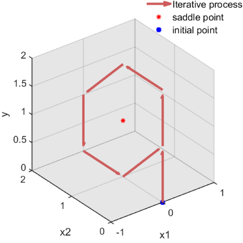
(a) AHPD ($\mu=\gamma=1$)

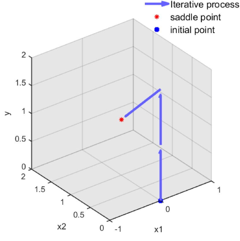
(b) FOPDA ($\mu=\gamma=1$)

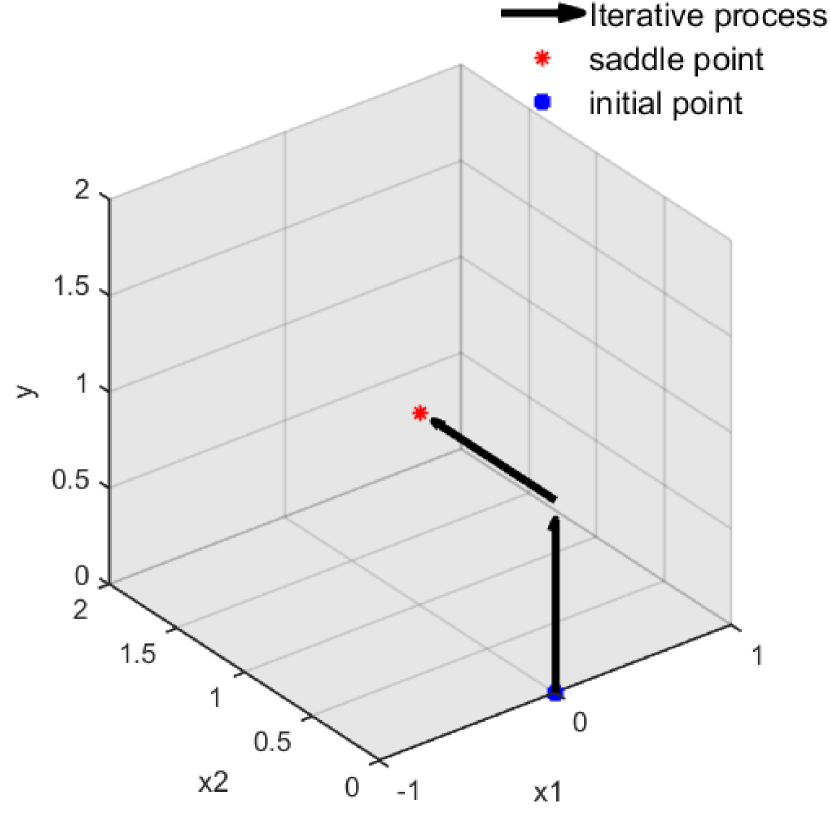
(c) Algorithm 1 ($\mu=\gamma=1$)

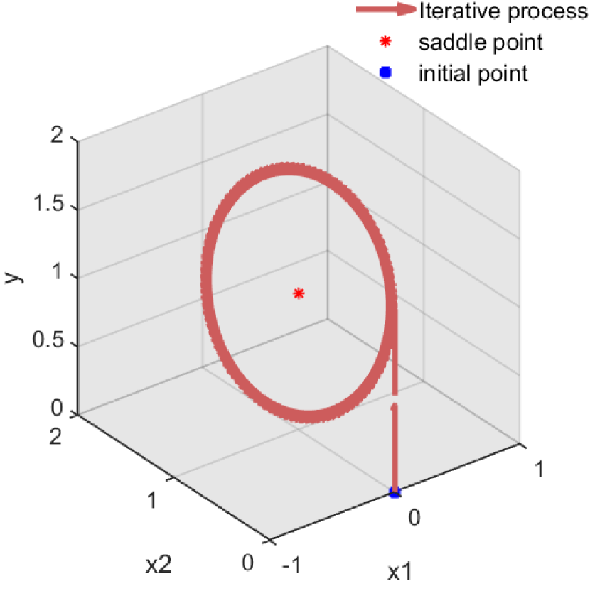
(d) AHPD ($\mu=\gamma=\sqrt{2}$)

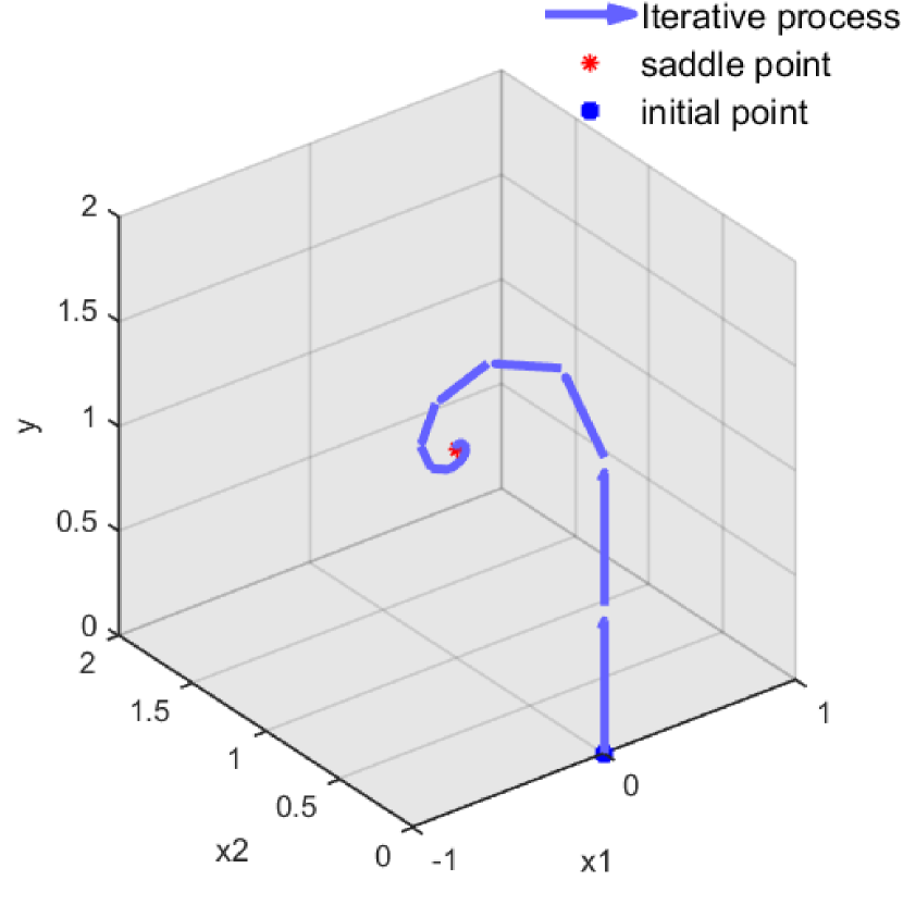
(e) FOPDA ($\mu=\gamma=\sqrt{2}$)

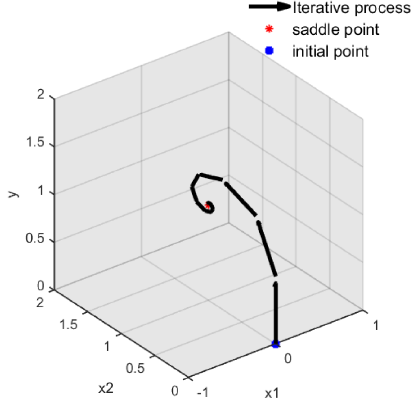
(f) Algorithm 1 ($\mu=\gamma=\sqrt{2}$)

Fig. 1: Illustration of the convergence behaviors of AHPD, FOPDA and Algorithm 1 for the toy example (14) with setting different parameters $\mu$ and $\gamma$.

Remark 2.

We employ a toy example used in [28] to show that our Algorithm 1 enjoys a nice convergence behavior. Consider the following linear programming:

(14) $$\min_{x_{1},x_{2}}\left\{\;2x_{1}+x_{2}\;|\;x_{1}+x_{2}=1,\;x_{1}\geq 0,\;x_{2}\geq 0\;\right\},$$

which has a unique solution $(x_{1}^{*},x_{2}^{*})=(0,1)$. Moreover, the dual problem of (14) is

$$\max_{y}\left\{\;y\;|\;y\leq 1,\;y\leq 2\;\right\}$$

and its optimal solution is $y^{*}=1$. Accordingly, we reformulate (14) as a standard form of saddle point problems, i.e.,

(15) $$\min_{x_{1}\geq 0,x_{2}\geq 0}\max_{y}\left\{\;2x_{1}+x_{2}-y\left(x_{1}+x_{2}-1\right)\;\right\}.$$

Applying Algorithm 1 to (15) with setting the Bregman kernel functions as the first type listed in Table 1, the iterative scheme is immediately specified as

$$\tilde{y}^{k+1}=y^{k}-\frac{1}{\gamma}\left(x^{k}_{1}+x^{k}_{2}-1\right),$$

$$x^{k+1}_{1}=\max\left\{\left(-\frac{2}{\mu}+\frac{1}{\mu}\tilde{y}^{k+1}+x_{1}^{k}\right),0\right\},$$

$$x^{k+1}_{2}=\max\left\{\left(-\frac{1}{\mu}+\frac{1}{\mu}\tilde{y}^{k+1}+x_{2}^{k}\right),0\right\},$$

$$y^{k+1}=y^{k}-\frac{1}{\gamma}\left(x^{k+1}_{1}+x^{k+1}_{2}-1\right).$$

Also, we implement the AHPD method (3) and the FOPDA (4) with $\tau=1$ to solve (15). Here, we take $(x^{0}_{1},x^{0}_{2},y^{0})=(0,0,0)$ as starting points and plot trajectories of the sequences generated by the three algorithms in Fig. 1 for the cases where $\mu=\gamma=1$ or $\mu=\gamma=\sqrt{2}$, respectively. It can be easily seen from Fig. 1 that the sequence generated by our Algorithm 1 converges slightly faster than FOPDA to the unique optimal solution, while the AHPD method generates a cyclic sequence. Such a toy example tells us that our Algorithm 1 possibly has superiority over some existing state-or-the-art primal-dual algorithms on some saddle point problems.

Remark 3.

When assuming that both $f(x)$ and $g(y)$ are differentiable, the saddle point problem (1) can be also reformulated as a standard variational inequality problem (VIP), i.e., finding a point ${\bm{u}}^{*}\in{\mathcal{U}}$ such that

(17) $$\langle{\bm{u}}-{\bm{u}}^{*},\nabla{\mathscr{L}}({\bm{u}}^{*})\rangle\geq 0,\quad\forall{\bm{u}}\in{\mathcal{U}},$$

where ${\bm{u}}$ and ${\mathcal{U}}$ are given in (9b), and $\nabla{\mathscr{L}}({\bm{u}})$ is specified as

$$\nabla{\mathscr{L}}({\bm{u}})=\left(\begin{array}[]{c}\nabla_{x}{\mathscr{L}}(x,y)\\ -\nabla_{y}{\mathscr{L}}(x,y)\end{array}\right)=\left(\begin{array}[]{c}\nabla f(x)+A^{\top}y\\ \nabla g(y)-Ax\end{array}\right).$$

Consequently, we can gainfully employ some efficient algorithms, such as the projection methods and extragradient methods (e.g., [46, 58]) tailored for VIPs to deal with those saddle point problems with differentiable objectives. However, many real-world problems does not necessarily satisfy the Lipschitz continuity of $\nabla{\mathscr{L}}({\bm{u}})$ required in convergence analysis. Besides, the aforementioned VIP-type methods such as the well-known extragradient methods (e.g., [46, 58]) treat both $x$ and $y$ as a whole, which possibly ignores the respective properties associated with both variables. As an usual consequence, when implementing the aforementioned extragradient methods, we must update $x$ and $y$ simultaneously, thereby reducing the implementability of extragradient methods for (1). Comparatively, our Algorithm 1 does not require the Lipschitz continuity of $\nabla{\mathscr{L}}({\bm{u}})$. More promisingly, our method is able to maximally exploit the structure of (1) so that each subproblem is easily implemented for many real-word problems (see Section 5).

Remark 4.

After we finished this manuscript, we are brought to the so-named Alternating Extragradient Method (AEM) introduced by Bonettini and Ruggiero [4, 6]. Under the same differentiability requirement on ${\mathscr{L}}(x,y)$, the AEM is an improved variant of the classical extragradient methods [46], where the respective structure associated with $x$ and $y$ can be efficiently explored. Moreover, the AEM enjoys an effective adaptive stepsize for primal and dual subproblems. However, the Lipschitz continuity assumption for the AEM would possibly preclude its applicability to some nonsmooth real-world problems. Comparatively, although our Algorithm 1 shares the same symmetric spirit to update the primal and dual variables with the AEM, our Algorithm 1 is applicable to nonsmooth saddle point problems with a bilinear coupling term. Moreover, as a theoretical complement, we not only prove the global convergence of Algorithm 1, but also estimate the linear convergence rate under the generalized error bound defined by Bregman distance.

3.2 Global convergence

In this subsection, we will prove the global convergence of Algorithm 1 under some standard conditions used in the primal-dual literature.

Note that both subproblems (11) and (13) share a similar form, so we denote

$${\bm{y}}_{w}=\arg\max_{y\in{\mathcal{Y}}}\left\{-g(y)+\langle Aw,y\rangle-\gamma\mathscr{B}_{\phi}(y,y^{k})\right\}$$

with some given $w\in{\mathbb{R}}^{m}$ for convenience, which can also be rewritten as

(18) $${\bm{y}}_{w}=\arg\min_{y\in{\mathcal{Y}}}\left\{g(y)-\langle Aw,y\rangle+\gamma\phi(y)-\gamma\langle\nabla\phi(y^{k}),y-y^{k}\rangle\right\}$$

Hereafter, we begin our analysis with the following lemma.

Lemma 5.

Suppose that the Bregman kernel function $\phi(\cdot)$ is $\varrho$-strongly convex. Let ${\bm{y}}_{u}$ and ${\bm{y}}_{w}$ be solutions of (18) for some given $u$ and $w$, respectively. Then, the following inequality

(19) $$g({\bm{y}}_{u})-g(y)+\langle{\bm{y}}_{u}-y,-Aw\rangle\leq \;\gamma\mathscr{B}_{\phi}(y,y^{k})-\gamma\mathscr{B}_{\phi}(y,{\bm{y}}_{w})-\gamma\mathscr{B}_{\phi}({\bm{y}}_{u},y^{k})$$

$$\;+\frac{\alpha\|A^{\top}A\|}{\varrho}\mathscr{B}_{\phi}(w,u)-(\gamma-\frac{1}{\alpha\varrho})\mathscr{B}_{\phi}({\bm{y}}_{w},{\bm{y}}_{u})$$

holds for all $y\in{\mathcal{Y}}$, where $\alpha$ is a positive constant.

Proof.

Note that ${\bm{y}}_{u}$ is a minimizer of (18) for given $u\in{\mathbb{R}}^{m}$. It then follows from the first-order optimality condition of (18) that

(20) $$g({\bm{y}}_{u})-g(y)\leq\langle y-{\bm{y}}_{u},-Au+\gamma\nabla\phi({\bm{y}}_{u})-\gamma\nabla\phi(y^{k})\rangle,\;\;\forall y\in{\mathcal{Y}}.$$

Consequently, by using the arbitrariness of $y$ in (20) with setting $y={\bm{y}}_{w}$, we have

(21) $$g({\bm{y}}_{u})-g({\bm{y}}_{w})\leq\langle{\bm{y}}_{w}-{\bm{y}}_{u},-Au+\gamma\nabla\phi({\bm{y}}_{u})-\gamma\nabla\phi(y^{k})\rangle.$$

Similarly, by the definition of ${\bm{y}}_{w}$, it then follows from the first-order optimality condition of (18) that

(22) $$g({\bm{y}}_{w})-g(y)\leq\langle y-{\bm{y}}_{w},-Aw+\gamma\nabla\phi({\bm{y}}_{w})-\gamma\nabla\phi(y^{k})\rangle,\;\;\forall y\in{\mathcal{Y}}.$$

Setting $y={\bm{y}}_{u}$ in (22) arrives at

(23) $$g({\bm{y}}_{w})-g({\bm{y}}_{u})\leq\langle{\bm{y}}_{u}-{\bm{y}}_{w},-Aw+\gamma\nabla\phi({\bm{y}}_{w})-\gamma\nabla\phi(y^{k})\rangle.$$

By invoking the definition of Bregman distance, we have

$$\gamma\mathscr{B}_{\phi}(y,y^{k})-\gamma\mathscr{B}_{\phi}(y,{\bm{y}}_{w})$$

$$=\gamma\phi({\bm{y}}_{w})-\gamma\phi(y^{k})+\gamma\langle\nabla\phi({\bm{y}}_{w}),y-{\bm{y}}_{w}\rangle-\gamma\langle\nabla\phi(y^{k}),y-y^{k}\rangle$$

(24) $$=\gamma\phi({\bm{y}}_{w})-\gamma\phi(y^{k})+\langle Aw,y-{\bm{y}}_{w}\rangle+\gamma\langle\nabla\phi(y^{k}),y^{k}-{\bm{y}}_{w}\rangle$$

$$\hskip 99.58464pt+\langle\gamma\nabla\phi({\bm{y}}_{w})-\gamma\nabla\phi(y^{k})-Aw,y-{\bm{y}}_{w}\rangle.$$

Using inequality (22) instead of the last term of (3.2) leads to

$$\gamma\mathscr{B}_{\phi}(y,y^{k})-\gamma\mathscr{B}_{\phi}(y,{\bm{y}}_{w})$$

$$\geq\gamma\phi({\bm{y}}_{w})-\gamma\phi(y^{k})+\langle Aw,y-{\bm{y}}_{w}\rangle+\gamma\langle\nabla\phi(y^{k}),y^{k}-{\bm{y}}_{w}\rangle+g({\bm{y}}_{w})-g(y)$$

$$=\gamma\phi({\bm{y}}_{w})-\gamma\phi(y^{k})+\langle Aw,{\bm{y}}_{u}-{\bm{y}}_{w}\rangle+\gamma\langle\nabla\phi(y^{k}),y^{k}-{\bm{y}}_{w}\rangle$$

$$\hskip 165.02606pt-\langle Aw,{\bm{y}}_{u}-y\rangle+g({\bm{y}}_{w})-g(y)$$

(25) $$=\Phi(y^{k},{\bm{y}}_{u},{\bm{y}}_{w})-\langle Aw,{\bm{y}}_{u}-y\rangle+g({\bm{y}}_{w})-g(y),$$

where

(26) $$\Phi(y^{k},{\bm{y}}_{u},{\bm{y}}_{w}):=\gamma\phi({\bm{y}}_{w})-\gamma\phi(y^{k})+\langle Aw,{\bm{y}}_{u}-{\bm{y}}_{w}\rangle+\gamma\langle\nabla\phi(y^{k}),y^{k}-{\bm{y}}_{w}\rangle.$$

Below, we focus on $\Phi(y^{k},{\bm{y}}_{u},{\bm{y}}_{w})$. First, we have

$$\langle Aw,{\bm{y}}_{u}-{\bm{y}}_{w}\rangle =\langle{\bm{y}}_{u}-{\bm{y}}_{w},Aw-Au\rangle+\langle{\bm{y}}_{u}-{\bm{y}}_{w},Au\rangle$$

$$=\langle{\bm{y}}_{u}-{\bm{y}}_{w},Aw-Au\rangle+\langle{\bm{y}}_{w}-{\bm{y}}_{u},\gamma\nabla\phi(y^{k})-\gamma\nabla\phi({\bm{y}}_{u})\rangle$$

$$\hskip 102.43008pt+\langle{\bm{y}}_{w}-{\bm{y}}_{u},-Au+\gamma\nabla\phi({\bm{y}}_{u})-\gamma\nabla\phi(y^{k})\rangle$$

(27) $$\geq\langle{\bm{y}}_{u}-{\bm{y}}_{w},Aw-Au\rangle+\langle{\bm{y}}_{w}-{\bm{y}}_{u},\gamma\nabla\phi(y^{k})-\gamma\nabla\phi({\bm{y}}_{u})\rangle$$

$$\hskip 102.43008pt+g({\bm{y}}_{u})-g({\bm{y}}_{w}),$$

where the last inequality follows from (21). As a result, substituting (3.2) into (26) immediately arrives at

$$\Phi(y^{k},{\bm{y}}_{u},{\bm{y}}_{w}) =\gamma\phi({\bm{y}}_{w})-\gamma\phi(y^{k})+\gamma\langle\nabla\phi(y^{k}),y^{k}-{\bm{y}}_{w}\rangle+\langle Aw,{\bm{y}}_{u}-{\bm{y}}_{w}\rangle$$

$$\geq\gamma\phi({\bm{y}}_{w})-\gamma\phi(y^{k})+\gamma\langle\nabla\phi(y^{k}),y^{k}-{\bm{y}}_{w}\rangle+\langle{\bm{y}}_{u}-{\bm{y}}_{w},Aw-Au\rangle$$

$$\hskip 48.36958pt+\langle{\bm{y}}_{w}-{\bm{y}}_{u},\gamma\nabla\phi(y^{k})-\gamma\nabla\phi({\bm{y}}_{u})\rangle+g({\bm{y}}_{u})-g({\bm{y}}_{w})$$

$$=\gamma\phi({\bm{y}}_{w})-\gamma\phi(y^{k})+\langle{\bm{y}}_{u}-{\bm{y}}_{w},Aw-Au\rangle-\langle\gamma\nabla\phi(y^{k}),{\bm{y}}_{u}-y^{k}\rangle$$

$$\hskip 48.36958pt-\langle\gamma\nabla\phi({\bm{y}}_{u}),{\bm{y}}_{w}-{\bm{y}}_{u}\rangle+g({\bm{y}}_{u})-g({\bm{y}}_{w})$$

(28) $$=\gamma\mathscr{B}_{\phi}({\bm{y}}_{w},{\bm{y}}_{u})+\gamma\mathscr{B}_{\phi}({\bm{y}}_{u},y^{k})+\langle{\bm{y}}_{u}-{\bm{y}}_{w},Aw-Au\rangle+g({\bm{y}}_{u})-g({\bm{y}}_{w}),$$

where the last equality follows from the definition of Bregman distance. Since the Bregman kernel function $\phi(\cdot)$ is $\varrho$-strongly convex and $\alpha>0$, we have

$$\langle{\bm{y}}_{u}-{\bm{y}}_{w},Aw-Au\rangle \geq-\frac{1}{2\alpha}\|{\bm{y}}_{w}-{\bm{y}}_{u}\|^{2}-\frac{\alpha}{2}\|A^{\top}A\|\|w-u\|^{2}$$

(29) $$\geq-\frac{1}{\alpha\varrho}\mathscr{B}_{\phi}({\bm{y}}_{w},{\bm{y}}_{u})-\frac{\alpha\|A^{\top}A\|}{\varrho}\mathscr{B}_{\phi}(w,u).$$

Plugging (3.2) into (3.2), we have

$$\Phi(y^{k},{\bm{y}}_{u},{\bm{y}}_{w})\geq\left(\gamma-\frac{1}{\alpha\varrho}\right)\mathscr{B}_{\phi}({\bm{y}}_{w},{\bm{y}}_{u})+\gamma\mathscr{B}_{\phi}({\bm{y}}_{u},y^{k})-\frac{\alpha\|A^{\top}A\|}{\varrho}\mathscr{B}_{\phi}(w,u)+g({\bm{y}}_{u})-g({\bm{y}}_{w}),$$

which, together with (3.2), implies that

$$\gamma\mathscr{B}_{\phi}(y,y^{k})-\gamma\mathscr{B}_{\phi}(y,{\bm{y}}_{w})$$

$$\geq\Phi(y^{k},{\bm{y}}_{u},{\bm{y}}_{w})-\langle Aw,{\bm{y}}_{u}-y\rangle+g({\bm{y}}_{w})-g(y)$$

$$\geq\left(\gamma-\frac{1}{\alpha\varrho}\right)\mathscr{B}_{\phi}({\bm{y}}_{w},{\bm{y}}_{u})+\gamma\mathscr{B}_{\phi}({\bm{y}}_{u},y^{k})-\frac{\alpha\|A^{\top}A\|}{\varrho}\mathscr{B}_{\phi}(w,u)$$

$$\hskip 108.12054pt+g({\bm{y}}_{u})-\langle Aw,{\bm{y}}_{u}-y\rangle-g(y).$$

Rearranging terms of the above inequality completes the proof. ∎

Lemma 6.

Let $\{(x^{k+1},\tilde{y}^{k+1},{y}^{k+1})\}$ be a sequence generated by Algorithm 1. Then, for all $x\in\mathcal{X}$ and $y\in\mathcal{Y}$, we have

(30) $${\mathscr{L}}(x^{k+1},y)- {\mathscr{L}}(x^{k+1},\tilde{y}^{k+1})$$

$$\leq\gamma\mathscr{B}_{\phi}(y,y^{k})-\gamma\mathscr{B}_{\phi}(y,y^{k+1})-\gamma\mathscr{B}_{\phi}(\tilde{y}^{k+1},y^{k})$$

$$\qquad+\frac{\alpha\|A^{\top}A\|}{\varrho}\mathscr{B}_{\phi}(x^{k+1},x^{k})-\left(\gamma-\frac{1}{\alpha\varrho}\right)\mathscr{B}_{\phi}(y^{k+1},\tilde{y}^{k+1})$$

and

(31) $${\mathscr{L}}(x^{k+1},\tilde{y}^{k+1})-{\mathscr{L}}(x,\tilde{y}^{k+1})\leq\mu\mathscr{B}_{\psi}(x,x^{k})-\mu\mathscr{B}_{\psi}(x,x^{k+1})-\mu\mathscr{B}_{\psi}(x^{k+1},x^{k}).$$

Proof.

First, it is clear from the notation in (1) that

(32) $${\mathscr{L}}(x^{k+1},y)-{\mathscr{L}}(x^{k+1},\tilde{y}^{k+1})=g(\tilde{y}^{k+1})-g(y)+\langle\tilde{y}^{k+1}-y,-Ax^{k+1}\rangle.$$

Since $\tilde{y}^{k+1}$ and $y^{k+1}$ are solutions of (11) and (13), respectively, it immediately follows from (32) and Lemma 5 with setting ${\bm{y}}_{u}=\tilde{y}^{k+1},{\bm{y}}_{w}=y^{k+1},u=x^{k},w=x^{k+1}$ that

$${\mathscr{L}}(x^{k+1},y)-{\mathscr{L}}(x^{k+1},\tilde{y}^{k+1}) =g(\tilde{y}^{k+1})-g(y)+\langle\tilde{y}^{k+1}-y,-Ax^{k+1}\rangle$$

$$\leq\gamma\mathscr{B}_{\phi}(y,y^{k})-\gamma\mathscr{B}_{\phi}(y,y^{k+1})-\gamma\mathscr{B}_{\phi}(\tilde{y}^{k+1},y^{k})$$

(33) $$\quad+\frac{\alpha\|A^{\top}A\|}{\varrho}\mathscr{B}_{\phi}(x^{k+1},x^{k})-\left(\gamma-\frac{1}{\alpha\varrho}\right)\mathscr{B}_{\phi}(y^{k+1},\tilde{y}^{k+1}),$$

which is precisely same as (30). We proved the first assertion of this lemma.

Below, we show (31). It follows from the notation of ${\mathscr{L}}(x,y)$ in (1) that

(34) $${\mathscr{L}}(x,\tilde{y}^{k+1})-{\mathscr{L}}(x^{k+1},\tilde{y}^{k+1})=f(x)-f(x^{k+1})+\langle Ax-Ax^{k+1},\tilde{y}^{k+1}\rangle.$$

One the other hand, the first-order optimality condition of (12) is

(35) $$f(x)-f(x^{k+1})+\left\langle x-x^{k+1},A^{\top}\tilde{y}^{k+1}+\mu\nabla\psi(x^{k+1})-\mu\nabla\psi(x^{k})\right\rangle\geq 0,\;\;\forall x\in{\mathcal{X}}.$$

Consequently, combining (34) and (35) leads to

$${\mathscr{L}}(x^{k+1},\tilde{y}^{k+1})-{\mathscr{L}}(x,\tilde{y}^{k+1}) =-f(x)+f(x^{k+1})-\langle Ax-Ax^{k+1},\tilde{y}^{k+1}\rangle$$

$$\leq\left\langle x-x^{k+1},\mu\nabla\psi(x^{k+1})-\mu\nabla\psi(x^{k})\right\rangle$$

(36) $$=-\mu\left\langle x-x^{k+1},\nabla\psi(x^{k})-\nabla\psi(x^{k+1})\right\rangle$$

Applying the three-point property of Bregman distance (7) to (3.2) with setting $a=x^{k+1}$, $b=x^{k}$, and $c=x$, we conclude that

$${\mathscr{L}}(x^{k+1},\tilde{y}^{k+1})-{\mathscr{L}}(x,\tilde{y}^{k+1}) \leq-\mu\langle x-x^{k+1},\nabla\psi(x^{k})-\nabla\psi(x^{k+1})\rangle$$

$$=\mu\mathscr{B}_{\psi}(x,x^{k})-\mu\mathscr{B}_{\psi}(x,x^{k+1})-\mu\mathscr{B}_{\psi}(x^{k+1},x^{k}).$$

This completes the proof of this lemma. ∎

Before presenting the global convergence theorem, we first make the following assumption. The Bregman kernel function $\phi(\cdot)$ associated with the $y$-subproblem is $\varrho$-strongly convex such that the proximal parameter $\gamma$ and constant $\alpha$ satisfying $\alpha\varrho\gamma\geq 1$. Moreover, there exists a constant $L$ satisfying $0<L\leq\frac{\varrho\mu}{\alpha\|A^{\top}A\|}$ such that the function $L\psi-\phi$ is convex, where $\psi(\cdot)$ is the Bregman kernel function associated with the $x$-subproblem.

Notice that, as shown in [2], the convexity of the function $L\psi-\phi$ is equivalent to

$$\phi(a)-\phi(b)-\langle\nabla\phi(b),a-b\rangle\leq L\mathscr{B}_{\psi}(a,b),\quad\forall a,b\in{\mathbb{R}}^{n},$$

which can also be rewritten as

(37) $$\mathscr{B}_{\phi}(a,b)\leq L\mathscr{B}_{\psi}(a,b),\quad\forall a,b\in{\mathbb{R}}^{n}.$$

Remark 5.

Note that the condition assumed in Assumption 3.2 is closely related to the standard requirements in [10]. First, the condition $\alpha\varrho\gamma\geq 1$ means that $\alpha\geq 1/(\varrho\gamma)$. Then, it follows that

$$L\leq\frac{\varrho\mu}{\alpha\|A^{\top}A\|}\leq\frac{\varrho^{2}\mu\gamma}{\|A^{\top}A\|},$$

which is same as the condition (5) when $L=\varrho=1.$

With the above preparations, we now state our global convergence theorem.

Theorem 7.

Suppose that Assumption 3.2 holds. Let $\{(x^{k+1},\tilde{y}^{k+1},{y}^{k+1})\}$ be a sequence generated by Algorithm 1. Then, for all $x\in{\mathcal{X}}$, $y\in{\mathcal{Y}}$, we have

$${\mathscr{L}}(\widehat{x}^{N},y)-{\mathscr{L}}(x,\widehat{y}^{N})\leq\frac{1}{N}\left(\gamma\mathscr{B}_{\phi}(y,y^{0})+\mu\mathscr{B}_{\psi}(x,x^{0})\right),$$

where $N$ is an positive integer, $\widehat{x}^{N}=\frac{1}{N}\sum_{k=0}^{N-1}x^{k}$ and $\widehat{y}^{N}=\frac{1}{N}\sum_{k=0}^{N-1}\tilde{y}^{k}$.

Proof.

Under Assumption 3.2, when $0<L\leq\frac{\varrho\mu}{\alpha\|A^{\top}A\|}$, the function $L\psi-\varphi$ is convex. It then follows from (37) and the definition of $\varphi(x)$ in Assumption 3.2 that

$$\mathscr{B}_{\psi}(x^{k+1},x^{k})\geq\frac{1}{L}\mathscr{B}_{\phi}(x^{k+1},x^{k})\geq\frac{\alpha\|A^{\top}A\|}{\varrho\mu}\mathscr{B}_{\phi}(x^{k+1},x^{k}),$$

which means that

(38) $$\mathscr{B}_{\Psi}(x^{k+1},x^{k})\geq 0\qquad\text{with}\quad\Psi:=\psi-\frac{\alpha\|A^{\top}A\|}{\varrho\mu}\phi.$$

Consequently, by adding (30) and (31), it follows from (38) and the positivity of the Bregman distance ($\alpha\varrho\gamma\geq 1$) that

$${\mathscr{L}}(x^{k+1},y)-{\mathscr{L}}(x,\tilde{y}^{k+1})\leq \gamma\mathscr{B}_{\phi}(y,y^{k})-\gamma\mathscr{B}_{\phi}(y,y^{k+1})+\mu\mathscr{B}_{\psi}(x,x^{k})-\mu\mathscr{B}_{\psi}(x,x^{k+1})$$

$$-\mu(\mathscr{B}_{\psi}(x^{k+1},x^{k})-\frac{\alpha\|A^{\top}A\|}{\varrho\mu}\mathscr{B}_{\phi}(x^{k+1},x^{k}))$$

$$-\gamma\mathscr{B}_{\phi}(\tilde{y}^{k+1},y^{k})-\left(\gamma-\frac{1}{\alpha\varrho}\right)\mathscr{B}_{\phi}(y^{k+1},\tilde{y}^{k+1})$$

$$\leq \gamma\mathscr{B}_{\phi}(y,y^{k})-\gamma\mathscr{B}_{\phi}(y,y^{k+1})+\mu\mathscr{B}_{\psi}(x,x^{k})-\mu\mathscr{B}_{\psi}(x,x^{k+1})$$

$$-\mu\mathscr{B}_{\Psi}(x^{k+1},x^{k})-\gamma\mathscr{B}_{\phi}(\tilde{y}^{k+1},y^{k})$$

$$-\left(\gamma-\frac{1}{\alpha\varrho}\right)\mathscr{B}_{\phi}(y^{k+1},\tilde{y}^{k+1})$$

(39) $$\leq \gamma\mathscr{B}_{\phi}(y,y^{k})-\gamma\mathscr{B}_{\phi}(y,y^{k+1})+\mu\mathscr{B}_{\psi}(x,x^{k})-\mu\mathscr{B}_{\psi}(x,x^{k+1}),$$

Hence, summing up (3.2) from $k=0$ to $N-1$ leads to

(40) $$\sum_{k=0}^{N-1}\left({\mathscr{L}}(x^{k+1},y)-{\mathscr{L}}(x,\tilde{y}^{k+1})\right)$$

$$\leq\gamma\mathscr{B}_{\phi}(y,y^{0})-\gamma\mathscr{B}_{\phi}(y,y^{N})+\mu\mathscr{B}_{\psi}(x,x^{0})-\mu\mathscr{B}_{\psi}(x,x^{N})$$

$$\leq\gamma\mathscr{B}_{\phi}(y,y^{0})+\mu\mathscr{B}_{\psi}(x,x^{0})$$

Notice that ${\mathscr{L}}(x,y)$ and $-{\mathscr{L}}(x,y)$ are convex with respect to $x$ and $y$, respectively. It then follows from the Jensen inequality and (40) that

$${\mathscr{L}}(\widehat{x}^{N},y)-{\mathscr{L}}(x,\widehat{y}^{N}) \leq\frac{1}{N}\sum_{k=0}^{N-1}\left({\mathscr{L}}(x^{k+1},y)-{\mathscr{L}}(x,\tilde{y}^{k+1})\right)$$

$$\leq\frac{1}{N}\left(\gamma\mathscr{B}_{\phi}(y,y^{0})+\mu\mathscr{B}_{\psi}(x,x^{0})\right).$$

We complete the proof of this theorem. ∎

Theorem 8.

Suppose that Assumption 3.2 holds. The sequence $\{(x^{k+1},{y}^{k+1})\}$ generated by Algorithm 1 converges to a saddle point of ${\mathscr{L}}(x,y)$ in (1).

Proof.

Letting $(x^{*},y^{*})$ be a saddle point of (1), we immediately have

(41) $${\mathscr{L}}(x^{*},y)\leq{\mathscr{L}}(x^{*},y^{*})\leq{\mathscr{L}}(x,y^{*}),\quad\forall x\in{\mathcal{X}},\;\forall y\in{\mathcal{Y}}.$$

On the other hand, by setting $x=x^{k+1}$ and $y=\tilde{y}^{k+1}$ in (41), it follows from (3.2) with settings $x=x^{*}$ and $y=y^{*}$ that

$$0 \leq{\mathscr{L}}(x^{k+1},y^{*})-{\mathscr{L}}(x^{*},\tilde{y}^{k+1})$$

$$\leq\gamma\mathscr{B}_{\phi}(y^{*},y^{k})-\gamma\mathscr{B}_{\phi}(y^{*},y^{k+1})+\mu\mathscr{B}_{\psi}(x^{*},x^{k})-\mu\mathscr{B}_{\psi}(x^{*},x^{k+1}),$$

which clearly implies that

(42) $$0\leq\gamma\mathscr{B}_{\phi}(y^{*},y^{k+1})+\mu\mathscr{B}_{\psi}(x^{*},x^{k+1})\leq\gamma\mathscr{B}_{\phi}(y^{*},y^{k})+\mu\mathscr{B}_{\psi}(x^{*},x^{k}).$$

Obviously, inequality (42) means that the sequence $\{\gamma\mathscr{B}_{\phi}(y^{*},y^{k})+\mu\mathscr{B}_{\psi}(x^{*},x^{k})\}$ is monotone decreasing and bounded. By the strong convexity of the Bregman distance, the sequence $\{(x^{k},y^{k})\}$ is bounded. Therefore, there exists a subsequence $\{(x^{k_{j}},y^{k_{j}})\}$ converging to a cluster point, denoted by $(x^{\infty},y^{\infty})$, which is also a cluster point of $\{(x^{k_{j}},\tilde{y}^{k_{j}})\}$. Below, we aim to show that such a cluster point is a saddle point of (1).

According to (3.2), we also have

$$\gamma\mathscr{B}_{\phi}(\tilde{y}^{k+1},y^{k})+\left(\gamma-\frac{1}{\alpha\varrho}\right)\mathscr{B}_{\phi}(y^{k+1},\tilde{y}^{k+1})+\mu\mathscr{B}_{\Psi}(x^{k+1},x^{k})$$

(43) $$\quad\leq\gamma\mathscr{B}_{\phi}(y^{*},y^{k})-\gamma\mathscr{B}_{\phi}(y^{*},y^{k+1})+\mu\mathscr{B}_{\psi}(x^{*},x^{k})-\mu\mathscr{B}_{\psi}(x^{*},x^{k+1}).$$

Summing the above inequality from $k=0$ to $N$, since $\alpha>0$, $\gamma>0$, $\mu>0$ and $\alpha\gamma\varrho\geq 1$ are constant, we have

$$\sum\limits_{k=0}^{N}\left(\gamma\mathscr{B}_{\phi}(\tilde{y}^{k+1},y^{k})+\left(\gamma-\frac{1}{\alpha\varrho}\right)\mathscr{B}_{\phi}(y^{k+1},\tilde{y}^{k+1})+\mu\mathscr{B}_{\Psi}(x^{k+1},x^{k})\right)$$

$$\leq\gamma\mathscr{B}_{\phi}(y^{*},y^{0})+\mu\mathscr{B}_{\psi}(x^{*},x^{0}),$$

which implies that

(44) $$\lim_{k\rightarrow\infty}\mathscr{B}_{\phi}(\tilde{y}^{k+1},y^{k})=\lim_{k\rightarrow\infty}\mathscr{B}_{\phi}(y^{k+1},\tilde{y}^{k+1})=\lim_{k\rightarrow\infty}\mathscr{B}_{\Psi}(x^{k+1},x^{k})=0.$$

It follows from the first-order optimality conditions of (12) and (13) that, for all $x\in{\mathcal{X}}$ and $y\in{\mathcal{Y}}$, the following inequalities hold

$$\left\{\begin{aligned} &f(x)-f(x^{k+1})+\left\langle x-x^{k+1},\;A^{\top}\tilde{y}^{k+1}+\mu\nabla\psi(x^{k+1})-\mu\nabla\psi(x^{k})\right\rangle\geq 0,\\ &g(y)-g(y^{k+1})+\left\langle y-y^{k+1},\;-Ax^{k+1}+\gamma\nabla\phi(y^{k+1})-\gamma\nabla\phi(y^{k})\right\rangle\geq 0.\end{aligned}\right.$$

Therefore, for all $x\in{\mathcal{X}}$ and $y\in{\mathcal{Y}}$, the subsequence $\{(x^{k_{j}},\tilde{y}^{k_{j}},y^{k_{j}})\}$ satisfies

(45) $$\left\{\begin{aligned} &f(x)-f(x^{k_{j}+1})+\left\langle x-x^{k_{j}+1},\;A^{\top}\tilde{y}^{k_{j}+1}+\mu\nabla\psi(x^{k_{j}+1})-\mu\nabla\psi(x^{k_{j}})\right\rangle\geq 0,\\ &g(y)-g(y^{k_{j}+1})+\left\langle y-y^{k_{j}+1},\;-Ax^{k_{j}+1}+\gamma\nabla\phi(y^{k_{j}+1})-\gamma\nabla\phi(y^{k_{j}})\right\rangle\geq 0.\end{aligned}\right.$$

Consequently, taking limit as $j\to\infty$ over the subsequence ${k_{j}}$ in (45), it follows from (44) that

$$\left\{\begin{aligned} &f(x)-f(x^{\infty})+\left\langle x-x^{\infty},\;A^{\top}y^{\infty}\right\rangle\geq 0,\quad\forall x\in{\mathcal{X}},\\ &g(y)-g(y^{\infty})+\left\langle y-y^{\infty},\;-Ax^{\infty}\right\rangle\geq 0,\quad\forall y\in{\mathcal{Y}},\end{aligned}\right.$$

which, together with (8), means that the limit point $(x^{\infty},y^{\infty})$ is a saddle point of ${\mathscr{L}}(x,y)$ in (1). So $(x^{*},y^{*})$ can be replaced by $(x^{\infty},y^{\infty})$ in the the sequence $\{\gamma\mathscr{B}_{\phi}(y^{*},y^{k})+\mu\mathscr{B}_{\psi}(x^{*},x^{k})\}$. Thus $\{\gamma\mathscr{B}_{\phi}(y^{\infty},y^{k})+\mu\mathscr{B}_{\psi}(x^{\infty},x^{k})\}$ is monotone decreasing and bounded, we obtain

$$\lim_{k\rightarrow\infty}\left(\gamma\mathscr{B}_{\phi}(y^{\infty},y^{k})+\mu\mathscr{B}_{\psi}(x^{\infty},x^{k})\right)=\lim_{j\rightarrow\infty}\left(\gamma\mathscr{B}_{\phi}(y^{\infty},y^{k_{j}})+\mu\mathscr{B}_{\psi}(x^{\infty},x^{k_{j}})\right)=0,$$

which means that $x^{k}\rightarrow x^{\infty}$ and $y^{k}\rightarrow y^{\infty}$ as $k\rightarrow\infty$. We complete the proof of this theorem. ∎

3.3 Linear convergence

In this subsection, we turn our attention to establishing the linear convergence in the context of a generalized error bound conditions. First, we make the following assumption, which is an extended version used in the literature, e.g., [36, 37, 54, 57].

Assume that, for any $\omega>0$, there exists $\eta>0$ such that

(46) $$\mathrm{\bf dist}_{\mathscr{B}}({\bm{u}},{\mathcal{U}}^{\star})\leq\eta\mathrm{\bf dist}(0,{\mathcal{E}}({\bm{u}},1)),\;\;\;\forall\|{\bm{u}}\|\leq\omega,\;{\bm{u}}\in{\mathcal{U}},$$

where ${\mathcal{E}}({\bm{u}},1)$ is given by (10) with $t=1$, and $\mathrm{\bf dist}_{\mathscr{B}}({\bm{u}},{\mathcal{U}}^{\star})$ is defined by

(47) $$\mathrm{\bf dist}_{\mathscr{B}}({\bm{u}},{\mathcal{U}}^{\star})=\min\left\{\sqrt{\mathscr{B}({\bm{u}}^{\star},{\bm{u}})}\;\big{|}\;{\bm{u}}^{\star}\in{\mathcal{U}}^{\star}\right\}$$

with $\mathscr{B}({\bm{u}}^{\star},{\bm{u}}):=\gamma\mathscr{B}_{\phi}(y^{\star},y)+\mu\mathscr{B}_{\psi}(x^{\star},x)$. Moreover, we assume that the gradients of $\psi(\cdot)$ and $\phi(\cdot)$ are Lipschitz continuous with modulus $L_{\psi}$ and $L_{\phi}$, respectively.

Hereafter, we establish the global linear convergence of Algorithm 1 under Assumption 3.3 in the context of generalized error bound condition defined by Bregman distance. We begin our analysis with the following lemma.

Lemma 9.

Let $\{(x^{k+1},\tilde{y}^{k+1},y^{k+1})\}$ be the sequence generated by Algorithm 1. Then, we have

(48) $$\mathrm{\bf dist}^{2}\left(0,{\mathcal{E}}({\bm{u}}^{k+1},1)\right) \leq 2\left(\|AA^{\top}\|+\gamma^{2}L_{\phi}^{2}\right)\|\tilde{y}^{k+1}-y^{k+1}\|^{2}$$

$$\qquad+2\mu^{2}L_{\psi}^{2}\|x^{k+1}-x^{k}\|^{2}+2\gamma^{2}L_{\phi}^{2}\left\|\tilde{y}^{k+1}-y^{k}\right\|^{2}.$$

where $L_{\phi}$ and $L_{\psi}$ are the Lipschitz continuous constants of $\nabla\phi(\cdot)$ and $\nabla\psi(\cdot)$, respectively.

Proof.

Letting $\xi^{k+1}\in\partial f(x^{k+1})$, it then follows from the first-order optimality condition of $x$-subproblem (12) that

$$x^{k+1}=\Pi_{{\mathcal{X}}}\left[x^{k+1}-\left(\xi^{k+1}-A^{\top}\tilde{y}^{k+1}+\mu\nabla\mathscr{B}_{\psi}(x^{k+1},x^{k})\right)\right],$$

which, together with the nonexpansiveness of projection operator $\Pi_{{\mathcal{X}}}(\cdot)$, implies that

$$\mathrm{\bf dist}^{2}\left(0,{\mathcal{E}}_{{\mathcal{X}}}({\bm{u}}^{k+1},1)\right) =\mathrm{\bf dist}^{2}\left(x^{k+1},\Pi_{{\mathcal{X}}}\left[x^{k+1}-(\xi^{k+1}+A^{\top}y^{k+1})\right]\right)$$

$$=\left\|\Pi_{{\mathcal{X}}}\left[x^{k+1}-\left(\xi^{k+1}+A^{\top}\tilde{y}^{k+1}+\mu\nabla\mathscr{B}_{\psi}(x^{k+1},x^{k})\right)\right]\right.$$

$$\hskip 113.81102pt\left.-\Pi_{{\mathcal{X}}}\left[x^{k+1}-(\xi^{k+1}+A^{\top}y^{k+1})\right]\right\|^{2}$$

$$\leq\left\|A^{\top}(y^{k+1}-\tilde{y}^{k+1})-\mu\nabla\mathscr{B}_{\psi}(x^{k+1},x^{k})\right\|^{2}$$

$$\leq 2\|AA^{\top}\|\left\|\tilde{y}^{k+1}-y^{k+1}\right\|^{2}+2\mu^{2}\left\|\nabla\mathscr{B}_{\psi}(x^{k+1},x^{k})\right\|^{2}$$

(49) $$\leq 2\|AA^{\top}\|\left\|\tilde{y}^{k+1}-y^{k+1}\right\|^{2}+2\mu^{2}L_{\psi}^{2}\left\|x^{k+1}-x^{k}\right\|^{2},$$

where the second inequality is derived by the fact that $\|a+b\|^{2}\leq 2a^{2}+2b^{2}$ holds for all $a,b\in{\mathbb{R}}^{n}$, and the last inequality follows from the Lipschitz continuity of $\nabla\psi(\cdot)$.

Similarly, it follows from the first-order optimality condition of the $y$-subproblem (13) that

$$y^{k+1}=\Pi_{{\mathcal{Y}}}\left[y^{k+1}-\left(\zeta^{k+1}-Ax^{k+1}+\gamma\nabla\mathscr{B}_{\phi}(y^{k+1},y^{k})\right)\right].$$

Then, we have

$$\mathrm{\bf dist}^{2}\left(0,{\mathcal{E}}_{{\mathcal{Y}}}({\bm{u}}^{k+1},1)\right) =\mathrm{\bf dist}^{2}\left(y^{k+1},\Pi_{{\mathcal{Y}}}\left[y^{k+1}-\left(\zeta^{k+1}-Ax^{k+1}\right)\right]\right)$$

$$=\left\|\Pi_{{\mathcal{Y}}}\left[y^{k+1}-\left(\zeta^{k+1}-Ax^{k+1}+\gamma\nabla\mathscr{B}_{\phi}(y^{k+1},y^{k})\right)\right]\right.$$

$$\hskip 113.81102pt\left.-\Pi_{{\mathcal{Y}}}\left[y^{k+1}-(\zeta^{k+1}-Ax^{k+1})\right]\right\|^{2}$$

$$\leq\gamma^{2}\left\|\nabla\mathscr{B}_{\phi}(y^{k+1},y^{k})\right\|^{2}$$

$$\leq\gamma^{2}L_{\phi}^{2}\left\|y^{k+1}-y^{k}\right\|^{2}$$

(50) $$\leq 2\gamma^{2}L_{\phi}^{2}\left\|y^{k+1}-\tilde{y}^{k+1}\right\|^{2}+2\gamma^{2}L_{\phi}^{2}\left\|\tilde{y}^{k+1}-y^{k}\right\|^{2}.$$

Consequently, combining (3.3) and (3.3) leads to

$$\mathrm{\bf dist}^{2}\left(0,{\mathcal{E}}({\bm{u}}^{k+1},1)\right)$$

$$=\mathrm{\bf dist}^{2}\left(0,{\mathcal{E}}_{{\mathcal{X}}}({\bm{u}}^{k+1},1)\right)+\mathrm{\bf dist}^{2}(0,{\mathcal{E}}_{{\mathcal{Y}}}\left({\bm{u}}^{k+1},1)\right)$$

$$\leq 2\left(\|AA^{\top}\|+\gamma^{2}L_{\phi}^{2}\right)\|\tilde{y}^{k+1}-y^{k+1}\|^{2}+2\mu^{2}L_{\psi}^{2}\|x^{k+1}-x^{k}\|^{2}+2\gamma^{2}L_{\phi}^{2}\left\|\tilde{y}^{k+1}-y^{k}\right\|^{2}.$$

Hence, the assertion of this lemma is obtained. ∎

Now, we establish the linear convergence rate of Algorithm 1 by the following theorem.

Theorem 10.

Let $\{(x^{k+1},\tilde{y}^{k+1},{y}^{k+1})\}$ be the sequence generated by Algorithm 1. Suppose that Assumption 3.3 holds. Then, we have

$$(1+\vartheta)\mathrm{\bf dist}_{\mathscr{B}}^{2}({\bm{u}}^{k+1},{\mathcal{U}}^{\star})\leq\mathrm{\bf dist}_{\mathscr{B}}^{2}({\bm{u}}^{k},{\mathcal{U}}^{\star}),$$

where $\vartheta$ is a constant given by

$$\vartheta=\min\left\{\;\frac{\varrho}{4\gamma\eta^{2}L_{\phi}^{2}},\;\frac{\gamma\alpha\varrho-1}{4\alpha\eta^{2}(\|AA^{\top}\|+\gamma^{2}L_{\phi}^{2})},\;\frac{\varsigma}{4\mu\eta^{2}L_{\psi}^{2}}\;\right\}>0.$$

Proof.

It first follows from (3.2) that

$$\gamma\mathscr{B}_{\phi}(y^{\star},y^{k+1})+\mu\mathscr{B}_{\psi}(x^{\star},x^{k+1}) \leq\gamma\mathscr{B}_{\phi}(y^{\star},y^{k})+\mu\mathscr{B}_{\psi}(x^{\star},x^{k})-\gamma\mathscr{B}_{\phi}(\tilde{y}^{k+1},y^{k})$$

(51) $$\quad-\left(\gamma-\frac{1}{\alpha\varrho}\right)\mathscr{B}_{\phi}(y^{k+1},\tilde{y}^{k+1})-\mu\mathscr{B}_{\Psi}(x^{k+1},x^{k}).$$

In accordance with Assumption 3.3, i.e., inequality (46), it follows from (48) that

$$\mathrm{\bf dist}_{\mathscr{B}}^{2}\left({\bm{u}}^{k+1},{\mathcal{U}}^{\star}\right) \leq\eta^{2}\mathrm{\bf dist}^{2}\left(0,{\mathcal{E}}({\bm{u}}^{k+1},1)\right),$$

(52) $$\leq\eta^{2}\left[2\left(\|AA^{\top}\|+\gamma^{2}L_{\phi}^{2}\right)\left\|\tilde{y}^{k+1}-y^{k+1}\right\|^{2}+2\mu^{2}L_{\psi}^{2}\left\|x^{k+1}-x^{k}\right\|^{2}\right.$$

$$\hskip 182.09746pt\left.+2\gamma^{2}L_{\phi}^{2}\left\|\tilde{y}^{k+1}-y^{k}\right\|^{2}\right].$$

Below, we let $\psi(\cdot)$ be $\varsigma$-strongly convex. Consequently, by the definition of $\mathrm{\bf dist}_{\mathscr{B}}({\bm{u}},{\mathcal{U}}^{\star})$ given by (47), we have

$$(1+\vartheta)\mathrm{\bf dist}_{\mathscr{B}}^{2}({\bm{u}}^{k+1},{\mathcal{U}}^{\star})$$

$$=\mathrm{\bf dist}_{\mathscr{B}}^{2}({\bm{u}}^{k+1},{\mathcal{U}}^{\star})+\vartheta\mathrm{\bf dist}_{\mathscr{B}}^{2}({\bm{u}}^{k+1},{\mathcal{U}}^{\star})$$

$$\leq\left[\gamma\mathscr{B}_{\phi}(y^{\star},y^{k+1})+\mu\mathscr{B}_{\psi}(x^{\star},x^{k+1})\right]+\vartheta\mathrm{\bf dist}_{\mathscr{B}}^{2}({\bm{u}}^{k+1},{\mathcal{U}}^{\star})$$

$$\leq\gamma\mathscr{B}_{\phi}(y^{\star},y^{k})+\mu\mathscr{B}_{\psi}(x^{\star},x^{k})$$

$$\quad-\gamma\mathscr{B}_{\phi}(\tilde{y}^{k+1},y^{k})-\left(\gamma-\frac{1}{\alpha\varrho}\right)\mathscr{B}_{\phi}(y^{k+1},\tilde{y}^{k+1})-\mu\mathscr{B}_{\Psi}(x^{k+1},x^{k})$$

$$\quad+\vartheta\eta^{2}\left[2\left(\|AA^{\top}\|+\gamma^{2}L_{\phi}^{2}\right)\left\|\tilde{y}^{k+1}-y^{k+1}\right\|^{2}+2\mu^{2}L_{\psi}^{2}\left\|x^{k+1}-x^{k}\right\|^{2}\right.$$

$$\hskip 199.16928pt\left.+2\gamma^{2}L_{\phi}^{2}\left\|\tilde{y}^{k+1}-y^{k}\right\|^{2}\right]$$

(53) $$\leq\gamma\mathscr{B}_{\phi}(y^{\star},y^{k})+\mu\mathscr{B}_{\psi}(x^{\star},x^{k})-\left[\frac{\gamma\varrho}{2}-2\vartheta\eta^{2}\gamma^{2}L_{\phi}^{2}\right]\left\|\tilde{y}^{k+1}-y^{k}\right\|^{2}$$

$$\quad-\left[\frac{\gamma\alpha\varrho-1}{2\alpha}-2\vartheta\eta^{2}\left(\|AA^{\top}\|+\gamma^{2}L_{\phi}^{2}\right)\right]\left\|\tilde{y}^{k+1}-y^{k+1}\right\|^{2}$$

$$\quad-\left[\frac{\mu\varsigma}{2}-2\vartheta\eta^{2}\mu^{2}L_{\psi}^{2}\right]\left\|x^{k+1}-x^{k}\right\|^{2},$$

where the second inequality is derived by (3.3), and the third inequality follows from the strong convexity of $\mathscr{B}_{\phi}$ and $\mathscr{B}_{\psi}$. As a consequence, by using the definition of $\vartheta$, inequality (3.3) implies that

(54) $$(1+\vartheta)\mathrm{\bf dist}_{\mathscr{B}}^{2}({\bm{u}}^{k+1},{\mathcal{U}}^{\star})\leq\gamma\mathscr{B}_{\phi}(y^{\star},y^{k})+\mu\mathscr{B}_{\psi}(x^{\star},x^{k})-\Gamma(x^{k+1},\tilde{y}^{k+1},y^{k+1}),$$

where $\Gamma(x^{k+1},\tilde{y}^{k+1},y^{k+1})$ is a positive term composed by the last three terms of (3.3). Then, setting $\mathrm{\bf dist}_{\mathscr{B}}^{2}({\bm{u}}^{k},{\mathcal{U}}^{\star})=\gamma\mathscr{B}_{\phi}(y^{\star},y^{k})+\mu\mathscr{B}_{\psi}(x^{\star},x^{k})$ in (54) immediately arrives at

$$(1+\vartheta)\mathrm{\bf dist}_{\mathscr{B}}^{2}({\bm{u}}^{k+1},{\mathcal{U}}^{\star})\leq\gamma\mathscr{B}_{\phi}(y^{\star},y^{k})+\mu\mathscr{B}_{\psi}(x^{\star},x^{k})=\mathrm{\bf dist}_{\mathscr{B}}^{2}({\bm{u}}^{k},{\mathcal{U}}^{\star}).$$

The assertion of this theorem is obtained. ∎

4 Applications to linearly constrained convex minimization

In this section, we shall show that our Algorithm 1 will reduce to some classical first-order algorithms, when applying linearly constrained convex optimization problems.

4.1 One-block case: Augmented Lagrangian method

In this subsection, we consider the following one-block convex minimization problem with linear constraints:

(55) $$\min_{x}\left\{\;f(x)\;|\;Ax=b,\;\;x\in{\mathcal{X}}\subseteq{\mathbb{R}}^{n}\right\},$$

where $f(\cdot):{\mathcal{X}}\to(-\infty,+\infty]$ is a proper closed convex function and $A\in{\mathbb{R}}^{m\times n}$ is a given matrix, and $b\in{\mathbb{R}}^{m}$ is a given vector. Accordingly, its augmented Lagrangian function reads as

(56) $${\mathscr{L}}_{\gamma}(x,y)=f(x)+\langle Ax-b,y\rangle+\frac{1}{2\gamma}\|Ax-b\|^{2},\quad\gamma>0,$$

and the augmented Lagrangian method for (55) is

$$\left\{\begin{aligned} x^{k+1}&=\arg\min_{x\in{\mathcal{X}}}\left\{f(x)+\langle Ax-b,y^{k}\rangle+\frac{1}{2\gamma}\|Ax-b\|^{2}\right\},\\ y^{k+1}&=y^{k}+\frac{1}{\gamma}(Ax^{k+1}-b).\end{aligned}\right.$$

or equivalently,

(57) $$\left\{\begin{aligned} x^{k+1}&=\arg\min_{x\in{\mathcal{X}}}\left\{f(x)+\frac{1}{2\gamma}\|Ax-b+\gamma y^{k}\|^{2}\right\},\\ y^{k+1}&=y^{k}+\frac{1}{\gamma}(Ax^{k+1}-b).\end{aligned}\right.$$

It is not difficult to observe that directly solving the $x$-subproblem in (57) is not an easy task (at least is not easily implementable), when $f(x)$ is a nonsmooth function (e.g., $\|x\|_{1}$ or nuclear norm for matrices) and $A$ is a general matrix, even for the case ${\mathcal{X}}={\mathbb{R}}^{n}$ (e.g., see [56]). Therefore, a natural way to make (57) implementable is linearizing the quadratic penalty term at $x^{k}$ as follows:

(58) $$\frac{1}{2\gamma}\|Ax-b\|^{2}\approx\frac{1}{2\gamma}\|Ax^{k}-b\|^{2}+\frac{1}{\gamma}\langle A^{\top}(Ax^{k}-b),x-x^{k}\rangle+\frac{\mu}{2}\|x-x^{k}\|^{2},$$

where $\mu\gamma\geq\|A^{\top}A\|$. Consequently, using the above approximation (58) instead of quadratic penalty term in (57), we immediately obtain the so-called Linearized Augmented Lagrangian Method (LALM) for (55), i.e.,

(59) $$\left\{\begin{aligned} x^{k+1}&=\arg\min_{x\in{\mathcal{X}}}\left\{f(x)+\frac{\mu}{2}\left\|x-\left(x^{k}+\frac{1}{\mu}A^{\top}\left(y^{k}+\frac{1}{\gamma}(Ax^{k}-b)\right)\right)\right\|^{2}\right\},\\ y^{k+1}&=y^{k}+\frac{1}{\gamma}(Ax^{k+1}-b).\end{aligned}\right.$$

When applying our Algorithm 1 to (55), we first reformulate (55) as the following saddle point problem:

(60) $$\min_{x\in{\mathcal{X}}}\max_{y\in{\mathbb{R}}^{m}}\left\{{\mathscr{L}}(x,y):=f(x)+\langle Ax,y\rangle-\langle b,y\rangle\right\}.$$

Then, the specific iterative scheme of Algorithm 1 for (60) reads as

(61) $$\left\{\begin{aligned} \tilde{y}^{k+1}&=\arg\max_{y\in{\mathbb{R}}^{m}}\left\{-\langle b,y\rangle+\langle Ax^{k},y\rangle-\gamma\mathscr{B}_{\phi}(y,y^{k})\right\},\\ x^{k+1}&=\arg\min_{x\in\mathcal{X}}\left\{f(x)+\langle Ax,\tilde{y}^{k+1}\rangle+\mu\mathscr{B}_{\psi}(x,x^{k})\right\},\\ y^{k+1}&=\arg\max_{y\in{\mathbb{R}}^{m}}\left\{-\langle b,y\rangle+\langle Ax^{k+1},y\rangle-\gamma\mathscr{B}_{\phi}(y,y^{k})\right\},\end{aligned}\right.$$

Clearly, by setting the Bregman kernel functions as $\phi(y)=\frac{1}{2}\|y\|^{2}$ and $\psi(x)=\frac{1}{2}\|x\|^{2}_{A^{\top}A}$, the iterative scheme (61) reads as

$$\left\{\begin{aligned} \tilde{y}^{k+1}&=\arg\max_{y\in{\mathbb{R}}^{m}}\left\{-\langle b,y\rangle+\langle Ax^{k},y\rangle-\frac{\gamma}{2}\|y-y^{k}\|^{2}\right\},\\ x^{k+1}&=\arg\min_{x\in\mathcal{X}}\left\{f(x)+\langle Ax,\tilde{y}^{k+1}\rangle+\frac{\mu}{2}\|Ax-Ax^{k}\|^{2}\right\},\\ y^{k+1}&=\arg\max_{y\in{\mathbb{R}}^{m}}\left\{-\langle b,y\rangle+\langle Ax^{k+1},y\rangle-\frac{\gamma}{2}\|y-y^{k}\|^{2}\right\},\end{aligned}\right.$$

which, by using the first-order optimality conditions of both $y$-subproblems, can be immediately simplified as

(62) $$\left\{\begin{aligned} \tilde{y}^{k+1}&=y^{k}+\frac{1}{\gamma}(Ax^{k}-b),\\ x^{k+1}&=\arg\min_{x\in\mathcal{X}}\left\{f(x)+\frac{\mu}{2}\left\|Ax-\left(Ax^{k}-\frac{1}{\mu}\tilde{y}^{k+1}\right)\right\|^{2}\right\},\\ y^{k+1}&=y^{k}+\frac{1}{\gamma}(Ax^{k+1}-b).\end{aligned}\right.$$

It is trivial that substituting $\tilde{y}^{k+1}$ into the update of $x^{k+1}$ and setting $\mu=1/\gamma$ immediately yields the ALM (57).

On the other hand, by setting the Bregman kernel functions as $\phi(y)=\frac{1}{2}\|y\|^{2}$ and $\psi(x)=\frac{1}{2}\|x\|^{2}$, the iterative scheme (61) reads as

$$\left\{\begin{aligned} \tilde{y}^{k+1}&=\arg\max_{y\in{\mathbb{R}}^{m}}\left\{-\langle b,y\rangle+\langle Ax^{k},y\rangle-\frac{\gamma}{2}\|y-y^{k}\|^{2}\right\},\\ x^{k+1}&=\arg\min_{x\in\mathcal{X}}\left\{f(x)+\langle Ax,\tilde{y}^{k+1}\rangle+\frac{\mu}{2}\|x-x^{k}\|^{2}\right\},\\ y^{k+1}&=\arg\max_{y\in{\mathbb{R}}^{m}}\left\{-\langle b,y\rangle+\langle Ax^{k+1},y\rangle-\frac{\gamma}{2}\|y-y^{k}\|^{2}\right\},\end{aligned}\right.$$

which, by using the first-order optimality conditions of both $y$-subproblems, can be immediately simplified as

(63) $$\left\{\begin{aligned} \tilde{y}^{k+1}&=y^{k}+\frac{1}{\gamma}(Ax^{k}-b),\\ x^{k+1}&=\arg\min_{x\in\mathcal{X}}\left\{f(x)+\frac{\mu}{2}\left\|x-\left(x^{k}-\frac{1}{\mu}A^{\top}\tilde{y}^{k+1}\right)\right\|^{2}\right\},\\ y^{k+1}&=y^{k}+\frac{1}{\gamma}(Ax^{k+1}-b).\end{aligned}\right.$$

Clearly, plugging the formula of $\tilde{y}^{k+1}$ into the update scheme of $x^{k+1}$ immediately yields the LALM (59).

It is interesting to notice that our algorithmic framework allows us to take different Bregman kernel functions. Therefore, we here follow the novel idea of the newly introduced balanced augmented Lagrangian method [31] to further consider taking $\phi(y)=\frac{1}{2}\|y\|^{2}_{(AA^{\top}+\kappa I)}$ and $\psi(x)=\frac{1}{2}\|x\|^{2}$ for model (55). Specifically, the concrete iterative scheme of Algorithm 1 reads as

(64) $$\left\{\begin{aligned} \tilde{y}^{k+1}&=y^{k}+\frac{1}{\gamma}(AA^{\top}+\kappa I)^{-1}(Ax^{k}-b),\\ x^{k+1}&=\arg\min_{x\in\mathcal{X}}\left\{f(x)+\frac{\mu}{2}\left\|x-\left(x^{k}-\frac{1}{\mu}A^{\top}\tilde{y}^{k+1}\right)\right\|^{2}\right\},\\ y^{k+1}&=y^{k}+\frac{1}{\gamma}(AA^{\top}+\kappa I)^{-1}(Ax^{k+1}-b),\end{aligned}\right.$$

where $(AA^{\top}+\kappa I)^{-1}$ can be efficiently calculated by the well-known Sherman-Morrison-Woodbury theorem, i.e., $(AA^{\top}+\kappa I)^{-1}=\kappa^{-1}\left(I_{n}-A(\kappa I_{m}+A^{\top}A)^{-1}A^{\top}\right)$ for the case where $m\ll n$. In what follows, we call the scheme (64) Doubly Balanced Augmented Lagrangian Method (DBALM). Moreover, when $f(x)$ is a quadratic function, i.e., $f(x)=\frac{1}{2}\|Bx-q\|^{2}$, we can also take $\psi(x)=\frac{1}{2}\|x\|^{2}_{(\tau I_{n}-B^{\top}B)}$ to derive a linearized version of DBALM to deal with the case where ${\mathcal{X}}$ is simple convex set whose projection is easily calculated.

4.2 Multi-block case: Jacobian splitting method

In this part, we are concerned with the multi-block linearly constrained convex minimization, which takes the form

(65) $$\min_{x_{1},x_{2},\ldots,x_{p}}\left\{\sum_{i=1}^{p}f_{i}(x_{i})\;\Big{|}\;\sum_{i=1}^{p}A_{i}x_{i}=b,\;\;x_{i}\in{\mathcal{X}}_{i}\subseteq{\mathbb{R}}^{n_{i}},\;i=1,2,\ldots,p\right\},$$

where $f_{i}(\cdot):\mathcal{X}_{i}\rightarrow(-\infty,+\infty]$ for $i=1,2,\cdots,p$ are proper closed convex functions, $A_{i}\in{\mathbb{R}}^{m\times n_{i}}$ are given matrices, and $b\in{\mathbb{R}}^{m}$ is a given vector. In the past decades, the multi-block model (65) has received much considerable attention due to its widespread applications in computer sciences and automatic control, e.g., see [22, 51]. Although such a model is also a linearly constrained optimization problem, it cannot be easily solved via the aforementioned ALM (57) since the linearly constraints make the ALM suffer from coupled subproblems so that the separability of the objective function cannot be fully exploited in algorithmic implementation. Accordingly, a series of augmented Lagrangian-based splitting methods were developed in the optimization literature, e.g., see [22, 23, 24, 27, 33, 55] and references therein.

Below, we first show that our Algorithm 1 is applicable to solving (65). In particular, we can easily derive that our Algorithm 1 is indeed the fully Jacobian splitting algorithm [27, 53] by choosing appropriate Bregman kernel functions. Moreover, we can obtain some new Jacobian splitting methods for (65).

First, it is clear that (65) can be rewritten into a compact form as follows:

(66) $$\min_{{\bm{x}}}\left\{{\bm{f}}({\bm{x}})\;|\;{\bm{A}}{\bm{x}}=b,\;\;{\bm{x}}\in{\mathcal{X}}\right\},$$

where ${\bm{x}}:=(x_{1}^{\top},x_{2}^{\top},\ldots,x_{p}^{\top})^{\top}$, ${\bm{f}}({\bm{x}}):=\sum_{i=1}^{p}f_{i}(x_{i})$, ${\bm{A}}:=[A_{1},A_{2},\ldots,A_{p}]$, and ${\mathcal{X}}:={\mathcal{X}}_{1}\times{\mathcal{X}}_{2}\times\ldots\times{\mathcal{X}}_{p}$. Therefore, we can reformulate (66) as the form of (60), i.e.,

(67) $$\min_{{\bm{x}}\in{\mathcal{X}}}\max_{y\in{\mathbb{R}}^{m}}\left\{{\mathscr{L}}({\bm{x}},y):={\bm{f}}({\bm{x}})+\left\langle{\bm{A}}{\bm{x}},y\right\rangle-\langle b,y\rangle\right\}.$$

Then, the specific iterative scheme of Algorithm 1 for (60) reads as

(68) $$\left\{\begin{aligned} \tilde{y}^{k+1}&=\arg\max_{y\in{\mathbb{R}}^{m}}\left\{-\langle b,y\rangle+\langle{\bm{A}}{\bm{x}}^{k},y\rangle-\gamma\mathscr{B}_{\phi}(y,y^{k})\right\},\\ {\bm{x}}^{k+1}&=\arg\min_{{\bm{x}}\in\mathcal{X}}\left\{{\bm{f}}({\bm{x}})+\langle{\bm{A}}{\bm{x}},\tilde{y}^{k+1}\rangle+\mu\mathscr{B}_{\psi}({\bm{x}},{\bm{x}}^{k})\right\},\\ y^{k+1}&=\arg\max_{y\in{\mathbb{R}}^{m}}\left\{-\langle b,y\rangle+\langle{\bm{A}}{\bm{x}}^{k+1},y\rangle-\gamma\mathscr{B}_{\phi}(y,y^{k})\right\}.\end{aligned}\right.$$

Now, we denote

$$M:=\left(\begin{array}[]{cccc}\beta_{1}A_{1}^{\top}A_{1}&0&\cdots&0\\ 0&\beta_{2}A_{2}^{\top}A_{2}&\cdots&0\\ \vdots&\vdots&\ddots&\vdots\\ 0&0&\cdots&\beta_{p}A_{p}^{\top}A_{p}\end{array}\right).$$

Then, by setting the Bregman kernel functions as $\phi(y)=\frac{1}{2}\|y\|^{2}$ and $\psi({\bm{x}})=\frac{1}{2}\|{\bm{x}}\|^{2}_{M}$ and using the separability of the objective function, for $\mu=1$, the iterative scheme (68) reads as

(69) $$\left\{\begin{aligned} \tilde{y}^{k+1}&=y^{k}+\frac{1}{\gamma}\left(\sum_{i=1}^{p}A_{i}x_{i}^{k}-b\right),\\ x_{i}^{k+1}&=\arg\min_{x_{i}\in{\mathcal{X}}_{i}}\left\{f_{i}(x_{i})+\frac{\mu}{2}\left\|Ax_{i}-\left(Ax_{i}^{k}-\frac{1}{\mu}\tilde{y}^{k+1}\right)\right\|^{2}\right\},\;i=1,\ldots,p,\\ y^{k+1}&=y^{k}+\frac{1}{\gamma}\left(\sum_{i=1}^{p}A_{i}x_{i}^{k+1}-b\right),\end{aligned}\right.$$

which actually corresponds to the proximal Jacobian splitting method studied in [27], especially precisely coincides with the augmented Lagrangian-based parallel splitting method [53] by setting $\beta_{i}=1/\gamma$ for $i=1,2\cdots,p$.

More interestingly, by setting the Bregman kernel functions as $\phi(y)=\frac{1}{2}\|y\|^{2}$ and $\psi({\bm{x}})=\frac{1}{2}\|{\bm{x}}\|^{2}$, the specific iterative scheme of Algorithm 1 for (67) reads as

(70) $$\left\{\begin{aligned} \tilde{y}^{k+1}&=y^{k}+\frac{1}{\gamma}\left(\sum_{i=1}^{p}A_{i}x_{i}^{k}-b\right),\\ x_{i}^{k+1}&=\arg\min_{x_{i}\in{\mathcal{X}}_{i}}\left\{f_{i}(x_{i})+\frac{\mu}{2}\left\|x_{i}-\left(x_{i}^{k}-\frac{1}{\mu}A_{i}^{\top}\tilde{y}^{k+1}\right)\right\|^{2}\right\},\;i=1,\ldots,p,\\ y^{k+1}&=y^{k}+\frac{1}{\gamma}\left(\sum_{i=1}^{p}A_{i}x_{i}^{k+1}-b\right),\end{aligned}\right.$$

which is a linearized parallel splitting method for (65). Comparing with the methods discussed in [20, 22, 24], the variant (70) enjoys relatively simpler iterative scheme without correction steps. Combining the ideas of (69) and (70), we can take

$$\widehat{M}:=\left(\begin{array}[]{cccccc}\beta_{1}A_{1}^{\top}A_{1}&\cdots&0&0&\cdots&0\\ \vdots&\ddots&\vdots&\vdots&\ddots&\vdots\\ 0&\cdots&\beta_{l}A_{l}^{\top}A_{l}&0&\cdots&0\\ 0&\cdots&0&\beta_{l+1}I&\cdots&0\\ \vdots&\ddots&\vdots&\vdots&\ddots&\vdots\\ 0&\cdots&0&0&\cdots&\beta_{p}I\end{array}\right)$$

so that $\phi(y)=\frac{1}{2}\|y\|^{2}$ and $\psi({\bm{x}})=\frac{1}{2}\|{\bm{x}}\|^{2}_{\widehat{M}}$, thereby producing a Partially Linearized Jacobian Splitting Method (PLJSM) for (65) with setting $\mu=1$, i.e.,

$$\left\{\begin{aligned} \tilde{y}^{k+1}&=y^{k}+\frac{1}{\gamma}\left(\sum_{i=1}^{p}A_{i}x_{i}^{k}-b\right),\\ x_{i}^{k+1}&=\arg\min_{x_{i}\in{\mathcal{X}}_{i}}\left\{f_{i}(x_{i})+\frac{\beta_{i}}{2}\left\|Ax_{i}-\left(Ax_{i}^{k}-\frac{1}{\beta_{i}}\tilde{y}^{k+1}\right)\right\|^{2}\right\},\;i=1,\ldots,l,\\ x_{j}^{k+1}&=\arg\min_{x_{j}\in{\mathcal{X}}_{j}}\left\{f_{j}(x_{j})+\frac{\beta_{j}}{2}\left\|x_{j}-\left(x_{j}^{k}-\frac{1}{\beta_{j}}A_{j}^{\top}\tilde{y}^{k+1}\right)\right\|^{2}\right\},\;j=l+1,\ldots,p,\\ y^{k+1}&=y^{k}+\frac{1}{\gamma}\left(\sum_{i=1}^{p}A_{i}x_{i}^{k+1}-b\right),\end{aligned}\right.$$

which, to our best knowledge, is not discussed in the literature. Of course, we can also follow the spirit of the DBALM (64) to specify $\phi(y)=\frac{1}{2}\|y\|^{2}_{(\sum_{i=1}^{p}A_{i}A_{i}^{\top}+\kappa I)}$ and $\psi({\bm{x}})=\frac{1}{2}\|{\bm{x}}\|^{2}_{\widehat{M}}$ to develop a doubly balanced PLJSM for (65).

5 Numerical experiments

In this section, we conduct the numerical performance of Algorithm 1 (denoted by SPIDA) on some well tested problems, including the matrix game, basis pursuit, RPCA, and image restoration with synthetic and real-world datasets. We also compare our Algorithm 1 with some existing state-of-the-art primal-dual-type algorithms for the purpose of showing the numerical improvement of our Algorithm 1. All algorithms are implemented in Matlab 2021a and all experiments are conducted on a 64-bit Windows personal computer with Intel(R) Core(TM) i5-12500h CPU@2.50GHz and 8GB of RAM.

5.1 Matrix games

We first consider a natural saddle point problem, which is called matrix game (see [12, 41]) and is used for approximately finding the Nash equilibrium of two-person zero-sum matrix games such as two-person Texas Hold’em Poker. Mathematically, such a min-max matrix game takes the form

$$\min_{x\in\Delta_{n}}\max_{y\in\Delta_{m}}\left\{{\mathscr{L}}(x,y)=\langle Ax,y\rangle\right\},$$

where $A\in\mathbb{R}^{m\times n}$, both sets $\Delta_{n}$ and $\Delta_{m}$ denote the standard unit simplices defined by

$$\Delta_{l}:=\left\{\;x\in{\mathbb{R}}^{l}\;\Big{|}\;\sum_{i=1}^{l}x_{i}=1,\;x_{i}\geq 0,\;i=1,2,\ldots,l\;\right\}.$$

To investigate the numerical behavior of our SPIDA, we compare SPIDA with the classical FOPDA (setting $\tau=1$ in (4)) and the recently introduced Golden Ratio Primal-Dual Algorithm (denoted by GRPDA) in [13]. As tested in [12], we here consider two random scenarios on matrix $A$: (i) all entries of $A$ are independently and uniformly distributed in the interval $[-1,1]$; (ii) all entries of $A$ are generated independently from the normal distribution $\mathcal{N}(0,1)$. For each scenario, we consider different sizes of $A$ as listed in Tables 2 and 3. To implement algorithms for solving this matrix game, we take $(\gamma,\mu)=(\|A\|,\|A\|)$ for FOPDA in (4), and take $(\psi,\tau,\sigma)=(1.618,\frac{\|A\|}{\sqrt{1.618}},\frac{\|A\|}{\sqrt{1.618}})$ for GRPDA. Additionally, we here consider Type I kernel function in Table 1 to equip Algorithm 1 and denote it by SPIDA, where the parameters are specified as $(\gamma,\mu)=(0.8\|A\|,0.8\|A\|)$ for experiments. It is pointing out that the projection onto unit simplex is calculated by the $n\log n$ algorithm described in [17]. All algorithms start with the same initial points $x_{0}=\frac{1}{n}(1,1,\cdots,1)^{\top}$ and $y_{0}=\frac{1}{m}(1,1,\cdots,1)^{\top}$, and stop at

(71) $$\text{Tol}:=\frac{\|(x^{k+1},y^{k+1})-(x^{k},y^{k})\|}{\|(x^{k},y^{k})\|}\leq\varepsilon.$$

In our experiments, we set $\varepsilon=10^{-4}$ and report the averaged performance of $10$ random trials. Specifically, we report the averaged number of iterations (Iter.), computing time in seconds (Time), and primal-dual gap (Gap) defined by

$$\text{Gap}:=\max_{i}(Ax)_{i}-\min_{j}(A^{\top}x)_{j}.$$

Some preliminary computational results are summarized in Tables 2 and 3, which show that our SPIDA takes relatively more computing time for larger scale cases than FOPDA and GRPDA, since SPIDA requires one more projection onto the simplex set at each iteration. However, SPIDA takes less iterations to achieve smaller primal-dual gaps than FOPDA and GRPDA, which support the reliability of the symmetric idea of this paper. Moreover, the convergence curves in Fig. 2 graphically show that our SPIDA has a nice convergence behavior.

Table 2: Numerical results for the matrix game: (i) Entries of $A$ are uniformly distributed in $[-1,1]$.

	FOPDA		GRPDA		SPIDA
$(n,m)$	Iter. / Time / Gap		Iter. / Time / Gap		Iter. / Time / Gap
$(100,100)$	1760.3 / 0.13 / 1.89$\times 10^{-4}$		1676.9 / 0.12 / 2.47$\times 10^{-4}$		1406.2 / 0.14 / 1.66$\times 10^{-4}$
$(100,500)$	1930.5 / 0.41 / 2.29$\times 10^{-4}$		2061.2 / 0.45 / 2.61$\times 10^{-4}$		1873.6 / 0.52 / 1.89$\times 10^{-4}$
$(100,1000)$	2434.3 / 1.09 / 2.88$\times 10^{-4}$		2317.9 / 1.01 / 3.14$\times 10^{-4}$		2180.6 / 1.21 / 2.21$\times 10^{-4}$
$(500,100)$	1953.4 / 0.45 / 2.23$\times 10^{-4}$		1923.1 / 0.44 / 2.69$\times 10^{-4}$		1771.6 / 0.55 / 1.93$\times 10^{-4}$
$(500,500)$	1456.0 / 5.81 / 1.27$\times 10^{-4}$		1611.2 / 6.38 / 1.42$\times 10^{-4}$		1284.7 / 8.44 / 1.03$\times 10^{-4}$
$(500,1000)$	1677.1 / 15.70 / 1.24$\times 10^{-4}$		1740.5 / 16.32 / 1.25$\times 10^{-4}$		1445.7 / 20.42 / 9.38$\times 10^{-5}$
$(1000,100)$	2430.1 / 1.05 / 2.77$\times 10^{-4}$		2816.4 / 1.22 / 3.26$\times 10^{-4}$		2181.4 / 1.38 / 2.24$\times 10^{-4}$
$(1000,500)$	1573.9 / 11.57 / 1.17$\times 10^{-4}$		1756.8 / 12.98 / 1.34$\times 10^{-4}$		1342.3 / 15.73 / 9.55$\times 10^{-5}$
$(1000,1000)$	1556.7 / 19.17 / 9.61$\times 10^{-5}$		1691.8 / 20.77 / 1.10$\times 10^{-4}$		1355.3 / 24.92 / 7.36$\times 10^{-5}$

Table 3: Numerical results for the matrix game: (ii) Entries of $A$ are normally distributed $\mathcal{N}(0,1)$.

	FOPDA		GRPDA		SPIDA
$(n,m)$	Iter. / Time / Gap		Iter. / Time / Gap		Iter. / Time / Gap
$(100,100)$	7181.2 / 0.58 / 5.67$\times 10^{-4}$		7456.7 / 0.62 / 6.57$\times 10^{-4}$		6229.8 / 0.77 / 4.45$\times 10^{-4}$
$(100,500)$	10283.0 / 3.22 / 7.95$\times 10^{-4}$		10474.7 / 3.32 / 9.50$\times 10^{-4}$		8807.2 / 3.57 / 6.44$\times 10^{-4}$
$(100,1000)$	11325.1 / 6.30 / 1.10$\times 10^{-3}$		11575.9 / 6.43 / 1.12$\times 10^{-3}$		9715.9 / 7.02 / 8.75$\times 10^{-4}$
$(500,100)$	9243.0 / 3.05 / 8.93$\times 10^{-4}$		10017.8 / 3.30 / 9.42$\times 10^{-4}$		7846.7 / 3.47 / 6.65$\times 10^{-4}$
$(500,500)$	10927.5 / 51.25 / 6.76$\times 10^{-4}$		11881.5 / 55.66 / 7.65$\times 10^{-4}$		9352.1 / 68.16 / 5.67$\times 10^{-4}$
$(500,1000)$	12843.0 / 103.04 / 7.79$\times 10^{-4}$		13559.4 / 108.93 / 8.75$\times 10^{-4}$		10956.1 / 129.11 / 6.04$\times 10^{-4}$
$(1000,100)$	11034.7 / 5.92 / 1.04$\times 10^{-3}$		12134.8 / 6.53 / 1.23$\times 10^{-3}$		9548.3 / 7.43 / 8.95$\times 10^{-4}$
$(1000,500)$	12561.7 / 83.05 / 7.51$\times 10^{-4}$		13805.0 / 91.22 / 8.43$\times 10^{-4}$		10697.9 / 110.27 / 6.10$\times 10^{-4}$
$(1000,1000)$	14152.8 / 184.09 / 7.86$\times 10^{-4}$		15438.1 / 200.60 / 8.15$\times 10^{-4}$		12159.1 / 234.59 / 6.11$\times 10^{-4}$

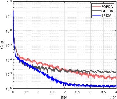
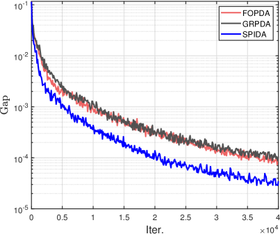
Fig. 2: Evolution of Primal-Dual Gap with respect to iterations for the matrix game. The left figure corresponds to the case where entries of $A\in{\mathbb{R}}^{500\times 100}$ are uniformly distributed in $[-1,1]$. The right one corresponds to the case where entries of $A\in{\mathbb{R}}^{100\times 500}$ are normally distributed in $\mathcal{N}(0,1)$.

5.2 Basis pursuit

As discussed in Section 4, our Algorithm 1 (SPIDA) is applicable to dealing with linearly constrained optimization problems (55). In this part, we are interested in the basis pursuit problem, which can be expressed mathematically as an $\ell_{1}$-norm minimization problem with linear constraints, i.e.,

(72) $$\min_{x\in{\mathbb{R}}^{n}}\;\left\{\;\|x\|_{1}\;|\;Ax=b\;\right\},$$

where $A\in\mathbb{R}^{m\times n}$ is a sample matrix and $b\in\mathbb{R}^{m}$ is a measurement vector. Such a model (72) is a fundamental problem in compressed sensing [16] and can be efficiently solved via a large number of optimization solvers. Here, we just employ this example to investigate the ability of our SPIDA on solving linearly constrained optimization problems, in addition to showing the superiority of SPIDA over some popular first-order optimization methods.

First, by the Lagrange function, we reformulate (72) as the following min-max saddle point problem:

$$\min_{x\in{\mathbb{R}}^{n}}\max_{y\in{\mathbb{R}}^{m}}\left\{\;{\mathscr{L}}(x,y)=\|x\|_{1}+\langle Ax,y\rangle-\langle b,y\rangle\;\right\}.$$

As compared in Section 5.1, we also compare our SPIDA with FOPDA (setting $\tau=1$ in (4)) and GRPDA [13]. Most recently, He and Yuan [31] introduced a novel Balanced Augmented Lagrangian Method (BALM) for linearly convex programming, which is a great improvement of the classical ALM (57). The iterative scheme of BALM for (72) reads as

(73) $$\left\{\begin{aligned} x^{k+1}&=\arg\min_{x\in{\mathbb{R}}^{n}}\left\{f(x)+\frac{\gamma}{2}\left\|x-\left(x^{k}-\frac{1}{\gamma}A^{\top}y^{k}\right)\right\|^{2}\right\},\\ y^{k+1}&=y^{k}+\left(\frac{1}{\gamma}AA^{\top}+\kappa I\right)^{-1}\left(A(2x^{k+1}-x^{k})-b\right).\end{aligned}\right.$$

In this part, we also compare our SPIDA with the BALM (73). Moreover, we will follow the idea of BALM to produce a doubly balanced augmented Lagrangian method (see (64) and denote it by SPIDA-II) via choosing the Type II Bregman kernel function in Table 1. As discussed in Section 4.1, when the Bregman kernel functions are specified as the Type I of Table 1, our SPIDA reduces to the LALM (59), which will be denoted by SPIDA-I in our numerical comparison.

In the experiments, we first construct a randomly $s$-sparse vector $x^{*}\in{\mathbb{R}}^{n}$, where $s$ is the number of nonzero components. Then, we randomly generate a sample matrix $A\in{\mathbb{R}}^{m\times n}$ to construct the measurement vector $b$ via $b=Ax^{*}$. Here, we consider two different ways to generate the sample matrix $A$:

• $A$ is a random Gaussian matrix;

• $A$ is a random partial DCT (discrete cosine transform) matrix.

We conduct different sizes of the problems by setting $(m,n,s)=(180i,960i,30i)$ with $i=1,2,\cdots,10$. Besides, to implement the algorithms, we take $(\gamma,\mu)=(1,1)$ for FOPDA, $(\psi,\tau,\sigma)=(2,\frac{\sqrt{2}}{2},\frac{\sqrt{2}}{2})$ for GRPDA, $(\gamma,\kappa)=(1.5,0.015)$ for BALM (73), $(\gamma,\mu)=(0.6,0.6)$ for SPIDA-I and $(\gamma,\mu,\kappa)=(0.6,0.6,0.01)$ for SPIDA-II. All algorithms start with zero initial points, and they are terminated when satisfying the stopping criterion (71) with $\varepsilon=10^{-6}$. Our summarized the averaged computational results of $10$ trials in Tables 4 and 5.

Table 4: Numerical results for basis pursuit: (i) $A$ is a random Gaussian matrix.

	FOPDA		GRPDA		BALM		SPIDA-I		SPIDA-II
$i$	Iter. / Time		Iter. / Time		Iter. / Time		Iter. / Time		Iter. / Time
$i=1$	689.5 / 1.36		587.5 / 1.16		292.6 / 0.60		348.3 / 0.70		167.6 / 0.41
$i=2$	1036.8 / 6.36		811.2 / 4.98		374.7 / 2.33		572.9 / 3.57		257.4 / 1.68
$i=3$	1525.3 / 16.20		1135.2 / 12.06		518.8 / 5.58		875.2 / 9.42		393.5 / 6.54
$i=4$	1595.8 / 27.53		1182.8 / 20.39		536.6 / 9.38		919.4 / 16.02		410.7 / 10.73
$i=5$	1295.3 / 31.37		980.6 / 23.78		451.2 / 11.19		737.3 / 18.03		335.9 / 11.96
$i=6$	3272.4 / 113.45		2346.8 / 81.19		1037.2 / 36.20		1938.0 / 67.91		887.9 / 42.56
$i=7$	1038.6 / 43.53		794.8 / 33.35		380.3 / 16.12		583.8 / 24.82		275.2 / 15.78
$i=8$	1567.3 / 85.37		1161.6 / 63.31		538.2 / 29.68		906.2 / 50.64		415.7 / 30.49
$i=9$	7314.6 / 472.55		5177.1 / 334.80		2389.7 / 155.92		4379.6 / 290.47		2073.1 / 179.49
$i=10$	8750.3 / 740.80		6198.3 / 527.87		2667.6 / 227.76		5238.9 / 450.59		2299.4 / 250.56

Table 5: Numerical results for basis pursuit: (ii) $A$ is a random partial DCT matrix.

	FOPDA		GRPDA		BALM		SPIDA-I		SPIDA-II
$i$	Iter. / Time		Iter. / Time		Iter. / Time		Iter. / Time		Iter. / Time
$i=1$	291.2 / 0.57		253.8 / 0.50		255.5 / 0.52		142.0 / 0.29		143.8 / 0.36
$i=2$	1278.4 / 8.21		901.5 / 5.77		873.4 / 5.63		756.0 / 4.95		763.8 / 5.46
$i=3$	397.0 / 4.61		325.0 / 3.76		322.3 / 3.77		207.9 / 2.43		210.1 / 3.79
$i=4$	1207.0 / 22.70		873.6 / 16.45		846.5 / 16.07		707.6 / 13.40		714.8 / 18.49
$i=5$	366.1 / 9.10		304.2 / 7.59		304.1 / 7.63		189.3 / 4.79		191.2 / 6.71
$i=6$	2558.8 / 91.87		1843.5 / 67.13		1781.4 / 65.38		1523.1 / 56.47		1538.3 / 73.30
$i=7$	1317.5 / 60.81		965.5 / 44.67		936.3 / 43.68		772.1 / 36.32		779.8 / 46.91
$i=8$	3931.9 / 231.36		2757.4 / 161.90		2658.5 / 157.81		2353.4 / 142.21		2376.7 / 181.08
$i=9$	631.7 / 45.56		482.6 / 34.82		471.0 / 34.29		357.9 / 26.63		361.6 / 33.40
$i=10$	1001.0 / 87.46		728.6 / 63.62		707.4 / 62.20		584.1 / 52.57		589.9 / 65.05

It can be easily seen from Table 4 that our SPIDA-II takes the fewest iterations to obtain approximate solutions for the case where $A$ is a random Gaussian matrix. When dealing with the other case where $A$ is a partial DCT matrix, results in Table 5 tell us that SPIDA-I and SPIDA-II have the almost same performance, while taking less iterations to achieve high-quality solutions than the other three first-order algorithms for (72). These computational results demonstrate that the symmetric updating way on the dual variable (i.e., twice calculations) equipped with a general proximal regularization can improve the numerical performance of the classical ALM. To further show the convergence behavior of our SPIDA, we focus on the case with $(m,n,s)=(360,1920,60)$ and plot the convergence curve of the relative error defined by ${\|x^{k}-x^{*}\|}/{\|x^{*}\|}$ with respect to iterations in Fig. 3. We see from Fig. 3 that our SPIDA has a promisingly linear convergence behavior for one-block linearly constrained optimization problems.

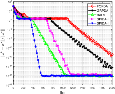
(a) Gaussian matrix

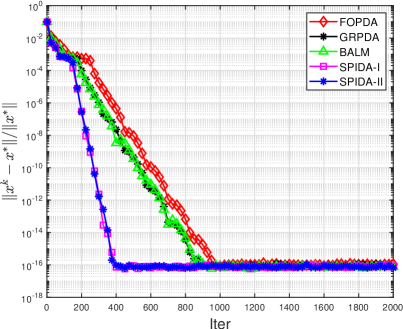
(b) partial DCT matrix

Fig. 3: Evolution of the relative error with respect to iterations for solving the basis pursuit problem (72).

5.3 RPCA

In this subsection, we give a numerical feedback to the applicability of our SPIDA to multi-block convex programming discussed in Section 4.2. Therefore, we consider a well-studied RPCA model [9], which refers to the task of recovering a sparse matrix and a low-rank one. Specifically, the RPCA under consideration takes the form

(74) $$\min_{X,Z}\;\left\{\;\|X\|_{*}+\lambda\|Z\|_{1}\;|\;X+Z=H\;\right\},$$

where $\|X\|_{*}$ is the nuclear norm (i.e., the sum of all singular values of $X$) for promoting the low-rankness of $X\in{\mathbb{R}}^{m\times n}$, $\|Z\|_{1}$ represents the $\ell_{1}$-norm for inducing the sparsity of $Z\in{\mathbb{R}}^{m\times n}$, and $H\in{\mathbb{R}}^{m\times n}$ is a given matrix. Obviously, the RPCA model (74) is a special case of the multi-block model (65) with two-block structure. Therefore, we can easily reformulate (74) as the following separable saddle point problem:

(75) $$\min_{X,Z}\max_{Y}\;\left\{\;{\mathscr{L}}(X,Z,Y)=\|X\|_{*}+\lambda\|Z\|_{1}+\langle X+Z,Y\rangle-\langle H,Y\rangle\;\right\}.$$

In this part, we also mainly compare SPIDA with FOPDA and GRPDA. Here, we consider the RPCA with synthetic and real data sets to verify the reliability of our algorithm for multi-block convex programming.

We first conduct the numerical performance of these algorithms on synthetic data sets. In this situation, we generate a low-rank matrix $X^{*}$ via $X^{*}=UV$, where $U\in{\mathbb{R}}^{n\times r}$ and $V\in{\mathbb{R}}^{r\times n}$ are independently random matrices whose entries are drawn from Gaussian distribution $\mathcal{N}(0,1)$. Then, we generate a sparse matrix $Z^{*}$ by randomly choosing a support set $\Omega$ of size $0.1\times n^{2}$ (i.e., $10\%$ nonzero components), and all elements are independently sampled from uniform distribution in $[-50,50]$. Finally, we let $H=X^{*}+Z^{*}$ be the observed matrix. Clearly, $(X^{*},Z^{*})$ is the true solution of (74). Throughout our experiments, we still employ the stopping criterion (71) with setting $\varepsilon=10^{-5}$ for all algorithms. Besides, we take $(\gamma,\mu)=(70.7107,0.0283)$ for FOPDA, $(\psi,\tau,\sigma)=(1.618,\frac{70.7107}{\sqrt{1.618}},\frac{0.0283}{\sqrt{1.618}})$ for GRPDA, $(\gamma,\mu)=(0.77*70.7107,0.0283)$ for SPIDA. In Table 6, we additionally report the rank of the obtained low-rank matrix ($\text{rank}(\hat{X})$), the number of nonzero components of the obtained sparse matrix ($\|\hat{Z}\|_{0}$), the relative error (Rerr) defined by

$$\text{Rerr}=\frac{\|\hat{X}+\hat{Z}-X^{*}-Z^{*}\|_{F}}{\|X^{*}+Z^{*}\|_{F}},$$

where $\hat{X}$ and $\hat{Z}$ respectively represent the low-rank and sparse matrices obtained by the algorithms. It can be seen from Table 6 that our SPIDA takes less iterations and computing time than both FOPDA and GRPDA to achieve almost the same low-rank and sparse separation on the observed matrix $H$.

Table 6: Numerical results of RPCA with synthetic data sets.

$(n,r)$	Methods	$\text{rank}(\hat{X})$	$\|\hat{Z}\|_{0}$	Rerr	Iter.	Time
$(256,13)$	FOPDA	13	6528	6.3011$\times 10^{-4}$	146	1.13
	GRPDA	13	6518	4.6516$\times 10^{-4}$	138	1.06
	SPIDA	13	6523	6.3007$\times 10^{-4}$	112	0.82
$(512,26)$	FOPDA	26	26143	1.2775$\times 10^{-4}$	127	4.73
	GRPDA	26	26151	1.1530$\times 10^{-4}$	119	4.50
	SPIDA	26	26128	1.7869$\times 10^{-4}$	86	3.23
$(1024,51)$	FOPDA	51	104677	7.0827$\times 10^{-5}$	78	14.32
	GRPDA	51	104725	5.0445$\times 10^{-5}$	87	15.48
	SPIDA	51	104677	7.0421$\times 10^{-5}$	61	10.88
$(2048,102)$	FOPDA	102	419106	2.4605$\times 10^{-5}$	80	269.52
	GRPDA	102	419221	1.7315$\times 10^{-5}$	105	378.50
	SPIDA	102	419106	2.4006$\times 10^{-5}$	67	205.77
$(2560,128)$	FOPDA	128	654970	1.6256$\times 10^{-5}$	93	299.85
	GRPDA	128	655097	1.5364$\times 10^{-5}$	124	383.87
	SPIDA	128	654965	1.5685$\times 10^{-5}$	80	248.64

Below, we are concerned with the numerical performance of SPIDA on RPCA with real data sets. So, we consider the application of model (74) in background separation of surveillance video. Here, we select three well-tested videos, i.e., Shoppingmall, Lobby, and Hall Airport, and select the first $200$ frames of each video to construct an observed matrix $H\in\mathbb{R}^{n\times 200}$, where $n=n_{1}\times n_{2}$ with $n_{1}$ and $n_{2}$ representing the height and width of the video, respectively. Notice that the true rank and sparsity of these videos are unknown. Therefore, we shall report the number of iterations, the computing time in seconds, the objective values (Obj.), and the error (Err.) defined by

$$\text{\sf Err}=\frac{\|\hat{X}+\hat{Z}-H\|_{F}}{\|H\|_{F}}.$$

Throughout, we set $\varepsilon=5\times 10^{-4}$ in (71) as the stopping tolerance for all algorithms. Computational results are summarized in Table 7, which also demonstrate that our SPIDA runs a little faster than both FOPDA and GRPDA for real-world data sets. In Fig. 4, we list the separated background and foreground of some frames. We can see from these results that all primal-dual-type algorithms are reliable for multi-block convex programming (65), especially for RPCA.

Table 7: Numerical results of RPCA with real-world data sets.

$(m,n)$	Methods	Obj.	Err.	Iter.	Time
Shoppingmall $(81920,200)$	FOPDA	3262.1	3.0359$\times 10^{-3}$	58	33.72
	GRPDA	3275.2	2.3097$\times 10^{-3}$	60	30.15
	SPIDA	3267.7	2.6796$\times 10^{-3}$	49	28.52
Lobby $(20480,200)$	FOPDA	969.65	4.1045$\times 10^{-3}$	128	13.53
	GRPDA	977.38	2.9694$\times 10^{-3}$	127	13.66
	SPIDA	973.61	3.5057$\times 10^{-3}$	109	11.58
Hall airport $(25344,200)$	FOPDA	2178.5	3.6816$\times 10^{-3}$	66	10.34
	GRPDA	2188.3	2.9182$\times 10^{-3}$	68	8.98
	SPIDA	2183.2	3.2527$\times 10^{-3}$	57	7.50

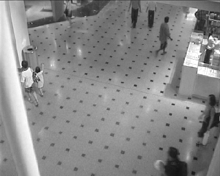
Fig. 4: Background and foreground separations of surveillance videos. Three lines of pictures from top to bottom correspond to the Hall airport, Lobby and Shoppingmall in the video. The first column corresponds to the 100th frame of the video. The second and third columns are the results extracted by FOPDA. The fourth and fifth columns are the results extracted by FOPDA.The last two columns are the results obtained by our SPIDA.

5.4 Image restoration

In this subsection, we apply the proposed SPIDA to solve an image restoration model with pixels constraints introduced in [21]. Such a model takes the form

(76) $$\min_{x\in\mathbb{B}}\;\left\{\||{\bm{D}}x|\|_{1}+\frac{\lambda}{2}\|Kx-b\|^{2}\;\right\},$$

where $\mathbb{B}$ is a box area characterizing the pixels of an image (indeed, $\mathbb{B}=[0,1]$ and $\mathbb{B}=[0,255]$ if the image are double precision and 8-bit gray scale, respectively); $\lambda$ is a positive trade-off parameter between the data-fidelity and regularization terms; $\bm{D}:=(\partial_{1},\partial_{2})$ denotes the gradient operator with $\partial_{1}$ and $\partial_{2}$ being the discretized derivatives in the horizontal and vertical directions, respectively; $K$ is the matrix representation of a blur operator and $b$ is a corrupted image with additive noise. Clearly, model (76) is equivalent to the following saddle point problem:

(77) $$\min_{x\in\mathbb{B}}\max_{y\in\mathbb{B}_{\infty}}\;\left\{\langle{\bm{D}}x,y\rangle+\frac{\lambda}{2}\|Kx-b\|^{2}\;\right\},$$

where $\mathbb{B}_{\infty}:=\left\{y\;|\;\|y\|_{\infty}\leq 1\right\}$. Consequently, when applying FOPDA (4) to (77), the iterative scheme is specified as

(78) $$\left\{\begin{aligned} y^{k+1}&=\arg\max_{y\in\mathbb{B}_{\infty}}\left\{\langle{\bm{D}}x^{k},y\rangle-\frac{\gamma}{2}\|y-y^{k}\|^{2}\right\}\equiv\Pi_{\mathbb{B}_{\infty}}(y^{k}+\gamma^{-1}\bm{D}x^{k}),\\ x^{k+1}&=\arg\min_{x\in\mathbb{B}}\left\{\frac{\lambda}{2}\|Kx-b\|^{2}+\langle{\bm{D}}x,2y^{k+1}-y^{k}\rangle+\frac{\mu}{2}\|x-x^{k}\|^{2}\right\},\end{aligned}\right.$$

where the updating order of $x$ and $y$ is exchanged due to the $y$-subproblem is simpler than the $x$-part, while the appearance of the deblurring matrix $K$ makes $x$-subproblem relatively difficult without closed-form solution. In this case, we employ the projected Barzilai-Borwein method in [15] and allow a maximal number of $50$ for the inner loop for finding an approximate solution of the $x$-subproblem in (78). To apply our SPIDA to (77), we consider two choices on the Bregman kernel functions: (i) $\psi(x)=\frac{1}{2}\|x\|^{2}$ and $\phi(y)=\frac{1}{2}\|y\|^{2}$; (ii) $\psi(x)=\frac{1}{2}\|x\|^{2}_{(I-\lambda\mu^{-1}K^{\top}K)}$ and $\phi(y)=\frac{1}{2}\|y\|^{2}$. In what follows, we denote our SPIDA equipped with the above two kernel functions by SPIDA-I and SPIDA-II, respectively. As a consequence, SPIDA-I and SPIDA-II are specified as

$$\text{(SPIDA-I)}\quad\left\{\begin{aligned} \tilde{y}^{k+1}&=\Pi_{\mathbb{B}_{\infty}}(y^{k}+\gamma^{-1}\bm{D}x^{k}),\\ x^{k+1}&=\arg\min_{x\in\mathbb{B}}\left\{\frac{\lambda}{2}\|Kx-b\|^{2}+\langle{\bm{D}}x,\tilde{y}^{k+1}\rangle+\frac{\mu}{2}\|x-x^{k}\|^{2}\right\},\\ y^{k+1}&=\Pi_{\mathbb{B}_{\infty}}(y^{k}+\gamma^{-1}\bm{D}x^{k+1}),\end{aligned}\right.$$

and

$$\text{(SPIDA-II)}\quad\left\{\begin{aligned} \tilde{y}^{k+1}&=\Pi_{\mathbb{B}_{\infty}}(y^{k}+\gamma^{-1}\bm{D}x^{k}),\\ x^{k+1}&=\Pi_{\mathbb{B}}\left(x^{k}-\lambda\mu^{-1}K^{\top}(Kx^{k}-b)-\mu^{-1}\bm{D}^{\top}\tilde{y}^{k+1}\right),\\ y^{k+1}&=\Pi_{\mathbb{B}_{\infty}}(y^{k}+\gamma^{-1}\bm{D}x^{k+1}).\end{aligned}\right.$$

We also employ the projected Barzilai-Borwein method to find an approximate solution of the $x$-subproblem of SPIDA-I.

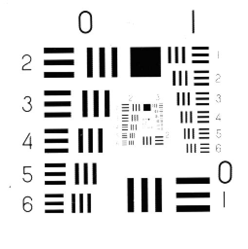
Fig. 5: From left to right: the original image, observed image corrupted by blurring kernel size $21\times 21$, recovered images by FOPDA, GRPDA, SPIDA-I and SPIDA-II, respectively.

In our experiments, we consider several widely tested images as listed in the first column of Fig. 5. These images are corrupted by the blur operator with $21\times 21$ uniform kernels. Then, the blurred images are further corrupted by adding the zero-white Gaussian noise with standard deviation $0.002$. The degraded images are listed in the second column of Fig. 5. We set $\varepsilon=10^{-4}$ in (77) as the stopping tolerance for all algorithms. The trade-off parameter $\lambda$ is specified as $\lambda=1000$. Moreover, we take $(\gamma,\mu)=(0.016,500)$ for FOPDA, $(\psi,\tau,\sigma)=(1.618,0.016,\frac{500}{1.618})$ for GRPDA, $(\gamma,\mu)=(0.016,0.75*500)$ for SPIDA-I and $(\gamma,\mu)=(0.016,500)$ for SPIDA-II. Some preliminary numerical results are summarized in Table 8, which clearly shows that our SPIDA-I and SPIDA-II perform better than FOPDA and GRPDA in terms of iterations and computing time. Note that SPIDA-I requires less iterations to achieve the almost same SNR values than SPIDA-II. However, SPIDA-II takes much less computing time than SPIDA-I, thanks to the closed-form solutions of SPIDA-II. These results efficiently support that our symmetric idea is able to improve the numerical performance of the original primal-dual algorithm.

Table 8: Numerical results for image restoration.

	FOPDA		GRPDA		SPIDA-I		SPIDA-II
image	Iter. / Time / SNR		Iter. / Time / SNR		Iter. / Time / SNR		Iter. / Time / SNR
chart	1476 / 16.37 / 19.214		1890 / 25.55 / 19.187		1217 / 15.12 / 19.220		1470 / 5.00 / 19.213
barbara	793 / 37.37 / 17.032		1035 / 59.67 / 17.036		677 / 36.64 / 17.029		792 / 15.73 / 17.032
mit	1080 / 13.11 / 12.960		1433 / 21.94 / 12.942		886 / 12.22 / 12.965		1078 / 3.81 / 12.960
flinstones	1141 / 54.02 / 14.439		1509 / 83.65 / 14.431		937 / 49.62 / 14.441		1171 / 23.47 / 14.440

In Fig. 5, we list the recovered images by FOPDA, GRPDA, SPIDA-I, and SPIDA-II from the third column to the last one, respectively. It can be seen that all methods are reliable to solve model (77). Finally, we list the evolution of SNR value with respect to computing time for solving image restoration model (77) in Fig. 6. These curves further show our SPIDA-II with easy subproblems has a superiority over the other algorithms in terms of computing time.

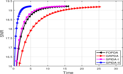
(a) chart

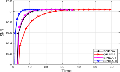
(b) barbara

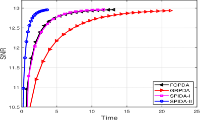
(c) mit

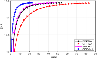
(d) flinstones

Fig. 6: Evolution of SNR value with respect to computing time for solving image restoration model (77).

6 Conclusions

In this paper, we proposed a new primal-dual algorithmic framework for convex-concave saddle point problems by applying the symmetric idea to compute the dual variable twice. Notice that a Bregman proximal regularization term is embedded in each subproblem, which is of benefit for us designing customized algorithms for some structured optimization problems. Moreover, we can gainfully understand the classical (linearized) augmented Lagrangian method and some parallel augmented Lagrangian-based splitting method for linearly constrained convex optimization. A series of experiments demonstrate that our new algorithm works better than the other two compared methods as long as the dual subproblem (i.e., $y$-subproblem) is easy enough with cheap computational cost. In future, we will consider some acceleration technique such as extrapolation on the method. Besides, we notice that all subproblems of our algorithm are required to be solved exactly, which is expensive or impossible in some cases (e.g., see experiments in matrix game and image restoration). Therefore, designing a practical inexact version of the proposed algorithm is also one of our future concerns.

References

- [1] K.J. Arrow, L. Hurwicz, and H. Uzawa, With contributions by H.B. Chenery, S.M. Johnson, S. Karlin, T. Marschak, and R.M. Solow. Studies in Linear and Non-Linear Programming, vol. II of Stanford Mathematical Studies in the Social Science, Stanford Unversity Press, Stanford, California, 1958.
- [2] H.H. Bauschke, J. Bolte, and M. Teboulle, A descent lemma beyond Lipschitz gradient continuity: first-order methods revisited and applications, Math. Oper. Res., 42 (2017), pp. 330–348.
- [3] A. Beck, First-Order Methods in Optimization, SIAM, Philadelphia, 2017.
- [4] S. Bonettini and V. Ruggiero, An alternating extragradientmethod for total variation based image restoration from Poisson data, Inverse Probl., 27 (2011), p. 095001.
- [5] , On the convergence of primal-dual hybrid gradient algorithms for total variation image restoration, J. Math. Imaging Vis., 44 (2012), pp. 236–253.
- [6] S. Bonettini and V. Ruggiero, An alternating extragradient method with non Euclidean projections for saddle point problems, Comput. Optim. Appl., 59 (2014), pp. 511–540.
- [7] L.M. Brègman, Relaxation method for finding a common point of convex sets and its application to optimization problems, in Doklady Akademii Nauk, vol. 171, Russian Academy of Sciences, 1966, pp. 1019–1022.
- [8] X.J. Cai, D.R. Han, and L.L. Xu, An improved first-order primal-dual algorithm with a new correction step, J. Global Optim., 57 (2013), pp. 1419–1428.
- [9] E.J. Candés, X.D. Li, Y. Ma, and J. Wright, Robust principal component analysis?, J. ACM, 58 (2011), pp. 1–37.
- [10] A. Chambolle and T. Pock, A first-order primal-dual algorithm for convex problems with applications to imaging, J. Math. Imaging Vis., 40 (2011), pp. 120–145.
- [11] , An introduction to continuous optimization for imaging, Acta Numer., 25 (2016), pp. 161–319.
- [12] , On the ergodic convergence rates of a first-order primal-dual algorithm, Math. Program. Ser. A, 159 (2016), pp. 253–287.
- [13] X.K. Chang and J.F. Yang, A golden ratio primal-dual algorithm for structured convex optimization, J. Sci. Comput., 87 (2021), p. 47.
- [14] X.K. Chang, J.F. Yang, and H.C. Zhang, Golden ratio primal-dual algorithm with linesearch, SIAM J. Optim., 32 (2022), pp. 1584–1613.
- [15] Y.H. Dai and R. Fletcher, Projected Barzilai-Borwein methods for large-scale box-constrained quadratic programming, Numer. Math., 100 (2005), pp. 21–47.
- [16] D. Donoho, Compressed sensing, IEEE Trans. Inform. Theory, 52 (2006), pp. 1289–1306.
- [17] J. Duchi, S. Shalev-Shwartz, Y. Singer, and T. Chandra, Efficient projections onto the l1-ball for learning in high dimensions, in Proceedings of the 25th International Conference on Machine Learning, ICML’08, 2008, pp. 272–279.
- [18] E. Esser, X. Zhang, and T. Chan, A general framework for a class of first-order primal-dual algorithms for convex optimization in imaging sciences, SIAM J. Imaging Sci., 3 (2010), pp. 1015–1046.
- [19] A. Fisher, Comments on: Critical Lagrange multipliers: what we currently know about them, how they spoil our lives, and what we can do about it, TOP, 23 (2015), pp. 27–31.
- [20] D.R. Han, H.J. He, and L.L. Xu, A proximal parallel splitting method for minimizing sum of convex functions, J. Comput. Appl. Math., 256 (2014), pp. 36–51.
- [21] D.R. Han, H.J. He, H. Yang, and X.M. Yuan, A customized Douglas-Rachford splitting algorithm for separable convex minimization with linear constraints, Numer. Math., 127 (2014), pp. 167–200.
- [22] D.R. Han, X.M. Yuan, and W.X. Zhang, An augmented-Lagrangian-based parallel splitting method for separable convex minimization with applications to image processing, Math. Comput., 83 (2014), pp. 2263–2291.
- [23] B.S. He, Parallel splitting augmented Lagrangian methods for monotone structured variational inequalities, Comput. Optim. Appl., 42 (2009), pp. 195–212.
- [24] B.S. He, L.S. Hou, and X.M. Yuan, On full Jacobian decomposition of the augmented lagrangian method for separable convex programming, SIAM J. Optim., 25 (2015), pp. 2274–2312.
- [25] B.S. He, F. Ma, S. Xu, and X.M. Yuan, A generalized primal-dual algorithm with improved convergence condition for saddle point problems, SIAM J. Imaging Sci., 15 (2022), pp. 1157–1183.
- [26] B.S. He, F. Ma, and X.M. Yuan, An algorithmic framework of generalized primal-dual hybrid gradient methods for saddle point problems., J Math. Imaging Vis., 58 (2017), pp. 279–293.
- [27] B.S. He, H.K. Xu, and X.M. Yuan, On the proximal Jacobian decomposition of ALM for multiple-block separable convex minimization problems and its relationship to ADMM, J. Sci. Comput., 66 (2016), pp. 1204–1217.
- [28] B.S. He, S.J. Xu, and X.M. Yuan, On convergence of the Arrow-Hurwicz method for saddle point problems, J. Math. Imaging Vis., 64 (2022), pp. 662–671.
- [29] B.S. He, Y.F. You, and X.M. Yuan, On the convergence of primal dual hybrid gradient algorithm, SIAM J. Imaging Sci., 7 (2015), pp. 2526–2537.
- [30] B.S. He and X.M. Yuan, Convergence analysis of primal-dual algorithms for a saddle-point problem: From contraction perspective, SIAM J. Imaging Sci., 5 (2012), pp. 119–149.
- [31] , Balanced augmented lagrangian method for convex programming, (2021). arXiv:2108.08554.
- [32] H.J. He, J. Desai, and K. Wang, A primal dual prediction correction algorithm for saddle point optimization, J. Global Optim., 66 (2016), pp. 573–583.
- [33] L.S. Hou, H.J. He, and J.F. Yang, A partially parallel splitting method for multiple-block separable convex programming with applications to robust PCA, Comput. Optim. Appl., 63 (2016), pp. 273–303.
- [34] A.F. Izmailov and M.V. Solodov, Critical Lagrange multipliers: what we currently know about them, how they spoil our lives, and what we can do about it, TOP, 23 (2015), pp. 1–26.
- [35] F. Jiang, X.J. Cai, Z.M. Wu, and D.R. Han, Approximate first-order primal-dual algorithms for saddle point problems, Math. Comput., 90 (2021), pp. 1227–1262.
- [36] F. Jiang, Z.M. Wu, X.J. Cai, and H.C. Zhang, A first-order inexact primal-dual algorithm for a class of convex-concave saddle point problems, Numer. Algor., 88 (2021), pp. 1109–1136.
- [37] F. Jiang, Z.Y. Zhang, and H.J. He, Solving saddle point problems: a landscape of primal-dual algorithm with larger stepsizes, J. Global Optim., (2022).
- [38] N. Komodakis and J. C. Pesquet, Playing with duality an overview of recent primal dual approaches for solving large scale optimization problems, IEEE Signal Process Mag., 32 (2015), pp. 31–54.
- [39] Y. Li and M. Yan, On the improved conditions for some primal-dual algorithms, (2022). arXiv:2201.00139v1.
- [40] Z. Li and M. Yan, New convergence analysis of a primal-dual algorithm with large stepsizes, Adv. Comput. Math., 47 (2021), pp. 1–20.
- [41] Y. Malitsky and T. Pock, A first-order primal-dual algorithm with linesearch, SIAM J. Optim., 28 (2018), pp. 411–432.
- [42] J.M. Martínez, Comments on: Critical Lagrange multipliers: what we currently know about them, how they spoil our lives, and what we can do about it, TOP, 23 (2015), pp. 35–42.
- [43] T. M’́ollenhoff, E. Strekalovskiy, M. Moeller, and D. Cremers, The primal dual hybrid gradient method for semiconvex splittings, SIAM J. Imaging Sci., 8 (2015), pp. 827–857.
- [44] B.S. Mordukhovich, Comments on: Critical Lagrange multipliers: what we currently know about them, how they spoil our lives, and what we can do about it, TOP, 23 (2015), pp. 35–42.
- [45] J.J. Moreau, Fonctions convexe dudual et points proximaux dans un espace hilbertien, C. R. Acad. Sci. Paris Ser. A Math, 255 (1962), pp. 2897–2899.
- [46] A. Nemirovski, Prox-method with rate of convergence for variational inequality with Lipschitz continuous monotone operators and smooth convex-concave saddle points problems, SIAM J. Optim., 15 (2004), pp. 229–251.
- [47] N. Parikh and S. Boyd, Proximal algorithms, Found. Trends Optim., 1 (2013), pp. 123–231.
- [48] J. Rasch and A. Chambolle, Inexact first-order primal–dual algorithms, Comput. Optim. Appl., 76 (2020), pp. 381–430.
- [49] M. Razaviyayn, T. Huang, S. Lu, M. Nouiehed, M. Sanjabi, and M. Hong, Nonconvex min-max optimization: Applications, challenges, and recent theoretical advances, IEEE Signal Process Mag., 37 (2020), pp. 55–66.
- [50] D.P. Robinson, Comments on: Critical Lagrange multipliers: what we currently know about them, how they spoil our lives, and what we can do about it, TOP, 23 (2015), pp. 43–47.
- [51] M. Tao and X.M. Yuan, Recovering low-rank and sparse components of matrices from incomplete and noisy observations, SIAM J. Optim., 21 (2011), pp. 57–81.
- [52] T. Valkonen, First-order primal–dual methods for nonsmooth non-convex optimisation, in Handbook of Mathematical Models and Algorithms in Computer Vision and Imaging: Mathematical Imaging and Vision, K. Chen, C.-B. Schönlieb, X.-C. Tai, and L. Younces, eds., Cham, 2021, Springer, pp. 1–42.
- [53] K. Wang, J. Desai, and H.J. He, A note on augmented Lagrangian-based parallel splitting method, Optim. Lett., 9 (2015), pp. 1199–1212.
- [54] K. Wang and H.J. He, A double extrapolation primal-dual algorithm for saddle point problems, J. Sci. Comput., 85 (2020), pp. 1–30.
- [55] X.F. Wang, M.Y. Hong, S.Q. Ma, and Z.Q. Luo, Solving multiple-block separable convex minimization problems using two-block alternating direction method of multipliers, Pac. J. Optim., 11 (2015), pp. 645–667.
- [56] J.F. Yang and X.M. Yuan, Linearized augmented Lagrangian and alternating direction methods for nuclear norm minimization, Math. Comput., 82 (2013), pp. 301–329.
- [57] W. Yang and D. Han, Linear convergence of the alternating direction method of multipliers for a class of convex optimization problems, SIAM J. Numer. Anal., 54 (2016), pp. 625–640.
- [58] H. Zhang, Extragradient and extrapolation methods with generalized Bregman distances for saddle point problems, Oper. Res. Lett., 50 (2022), pp. 329–334.
- [59] M.Q. Zhu and T. Chan, An efficient primal-dual hybrid gradient algorithm for total variation image restoration, CAM Reports 08-34, UCLA, 2008.