Faster Maximum Inner Product Search in High Dimensions

Abstract

Maximum Inner Product Search (MIPS) is a ubiquitous task in machine learning applications such as recommendation systems. Given a query vector and $n$ atom vectors in $d$-dimensional space, the goal of MIPS is to find the atom that has the highest inner product with the query vector. Existing MIPS algorithms scale at least as $O(\sqrt{d})$, which becomes computationally prohibitive in high-dimensional settings. In this work, we present BanditMIPS, a novel randomized MIPS algorithm whose complexity is independent of $d$. BanditMIPS estimates the inner product for each atom by subsampling coordinates and adaptively evaluates more coordinates for more promising atoms. The specific adaptive sampling strategy is motivated by multi-armed bandits. We provide theoretical guarantees that BanditMIPS returns the correct answer with high probability, while improving the complexity in $d$ from $O(\sqrt{d})$ to $O(1)$. We also perform experiments on four synthetic and real-world datasets and demonstrate that BanditMIPS outperforms prior state-of-the-art algorithms. For example, in the Movie Lens dataset ($n$=4,000, $d$=6,000), BanditMIPS is 20$\times$ faster than the next best algorithm while returning the same answer. BanditMIPS requires no preprocessing of the data and includes a hyperparameter that practitioners may use to trade off accuracy and runtime. We also propose a variant of our algorithm, named BanditMIPS-$\alpha$, which achieves further speedups by employing non-uniform sampling across coordinates. Finally, we demonstrate how known preprocessing techniques can be used to further accelerate BanditMIPS, and discuss applications to Matching Pursuit and Fourier analysis.

1 Introduction

The Maximum Inner Product Search problem (MIPS) [84, 79, 99] is a ubiquitous task that arises in many machine learning applications, such as matrix-factorization-based recommendation systems [61, 30], multi-class prediction [33, 50], structural SVM [54, 55], and computer vision [33]. Given a query vector $\mathbf{q}\in\mathbb{R}^{d}$ and $n$ atom vectors $\mathbf{v}_{1},\ldots,\mathbf{v}_{n}\in\mathbb{R}^{d}$, MIPS aims to find the atom most similar to the query:

$$i^{*}=\operatorname*{arg\,max}_{i\in\{1,\cdots,n\}}\mathbf{v}_{i}^{T}\mathbf{q}$$ (1)

For example, in recommendation systems, the query $\mathbf{q}$ may represent a user and the atoms $\mathbf{v}_{i}$’s represent items with which the user can interact; MIPS finds the best item for the user, as modeled by their concordance $\mathbf{v}_{i}^{T}\mathbf{q}$ [3, 6]. In many applications, the number of atoms $n$ and the feature dimension $d$ can easily be in the millions, so it is critical to solve MIPS accurately and efficiently [46].

The naïve approach evaluates all $nd$ elements and scales as $O(nd)$. Most recent works focus on reducing the scaling with $n$ and scale at least linearly in $d$ [66], which may be prohibitively slow in high-dimensional settings. [64] proposed a sampling-based approach that improved the complexity to $O(n\sqrt{d})$. In this work, we focus on further improving the complexity with respect to $d$ and providing a tunable hyperparameter that governs the tradeoff between accuracy and speed, a need identified by previous works [99].

We propose BanditMIPS, a new randomized algorithm for MIPS whose complexity is independent of $d$. We provide theoretical guarantees that BanditMIPS recovers the exact solution to Equation (1) with high probability in $\tilde{O}(\frac{n}{\Delta^{2}})$ time, where $\Delta$ is an instance-specific factor that does not depend on $d$. We have also performed comprehensive experiments to evaluate our algorithm’s performance in two synthetic and two real-world datasets. For example, in the Movie Lens dataset ($n=4,000$, $d=6,000$) [45], BanditMIPS is 20$\times$ faster than prior state-of-the-art while returning the same answer.

At a high-level, instead of computing the inner product $\mathbf{v}_{i}^{T}\mathbf{q}$ for each atom $i$ using all $d$ coordinates, BanditMIPS estimates them by subsampling a subset of coordinates. Since more samples give higher estimation accuracy, BanditMIPS adaptively samples more coordinates for top atoms to discern the best atom. The specific adaptive sampling procedure is motivated by multi-armed bandits (MAB) [39].

BanditMIPS is easily parallelizable and can be used with other optimization objectives that decompose coordinate-wise. Unlike previous works, it does not require preprocessing or normalization of the data, nor does it require the query or atoms to be nonnegative [99]. BanditMIPS also has a tunable hyperparameter to trade off accuracy and speed. We also developed several extensions of BanditMIPS. First, we propose BanditMIPS-$\alpha$, which provides additional runtime speedups by sampling coordinates intelligently in Section 3.1. Second, we extend BanditMIPS to find the $k$ atoms with the highest inner products with the query ($k$-MIPS) in our experiments in Section 5 and Appendix 10. Third, we discuss how BanditMIPS can be used in conjunction with preprocessing techniques in Appendix 11 and examples of downstream applications in Appendix 12.

1.1 Related work

MIPS applications: MIPS arises naturally in many information retrieval contexts [87, 35, 23] and for augmenting large, auto-regressive language models [19]. MIPS is also a subroutine in the Matching Pursuit problem (MP) and its variants, such as Orthogonal Matching Pursuit (OMP) [65]. MP and other iterative MIPS algorithms have found a many applications, e.g., to find a sparse solution of underdetermined systems of equations [36] and accelerate conditional gradient methods [89, 97]. MIPS also arises in the inference stages of many other applications, such as for deep-learning based multi-class or multi-label classifiers [33, 50] and has been used as a black-box subroutine to improve the learning and inference in unnormalized log-linear models when computing the partition function is intractable [77].

MIPS algorithms: Many approaches focus on solving approximate versions of MIPS. Such work often assumes that the vector entries are nonnegative, performs non-adaptive sampling [69, 15, 66, 34, 99], or rely on product quantization [31, 95, 44, 43, 73, 37, 42, 8, 58, 57]. Many of these algorithms require significant preprocessing, are limited in their adaptivity to the underlying data distribution, provide no theoretical guarantees, or scale linearly in $d$—all drawbacks that have been identified as bottlenecks for MIPS in high dimensions [83].

A large family of MIPS algorithms are based on locality-sensitive hashing (LSH) [49, 84, 86, 79, 47, 88, 68, 85, 94, 48, 70, 5, 98]. A shortcoming of these LSH-based approaches is that, in high dimensions, the maximum dot product is often small compared to the vector norms, which necessitates many hashes and significant storage space (often orders of magnitude more than the data itself). Many other MIPS approaches are based on proximity graphs, such as ip-NSW [75] and related work [63, 41, 92, 91, 103, 29, 102, 2, 71, 72]. These approaches use preprocessing to build an index data structure that allows for more efficient MIPS solutions at query time. However, these approaches also do not scale well to high dimensions as the index structure (an approximation to the true proximity graph) breaks down due to the curse of dimensionality [63].

Perhaps most similar to our work is BoundedME [64]. Similar to our method, their approach presents a solution to MIPS based on adaptive sampling but scales as $O(n\sqrt{d})$, worse than our algorithm that does not scale with $d$. This is because in BoundedME, the number of times each atom is sampled is predetermined by $d$ and not adaptive to the actual values of the sampled inner products; rather, is only adaptive to their relative ranking. Intuitively, this approach is wasteful because information contained in the sampled inner product’s values is discarded.

Additional related work is discussed in Appendix 7.

Multi-armed bandits: BanditMIPS is motivated by the best-arm identification problem in multi-armed bandits [39, 60, 7, 52, 51, 53, 25, 16, 20, 38, 59]. In a typical setting, we have $n$ arms each associated with an expected reward $\mu_{i}$. At each time step $t=0,1,\cdots,$ we decide to pull an arm $A_{t}\in\{1,\cdots,n\}$, and receive a reward $X_{t}$ with $E[X_{t}]=\mu_{A_{t}}$. The goal is to identify the arm with the largest reward with high probability while using the fewest number of arm pulls. The use of MAB-based adaptive sampling to develop computationally efficient algorithms has seen many applications, such as random forests and $k$-medoid clustering [93, 11, 12, 100, 10].

2 Preliminaries and Notation

We consider a query $\mathbf{q}\in\mathbb{R}^{d}$ and $n$ atoms $\mathbf{v}_{1},\ldots,\mathbf{v}_{n}\in\mathbb{R}^{d}$. Let $[n]$ denote $\{1,\ldots,n\}$, $q_{j}$ the $j$th element of $\mathbf{q}$, and $v_{ij}$ the $j$th element of $\mathbf{v}_{i}$. For a given query $\mathbf{q}\in\mathbb{R}^{d}$, the MIPS problem is to find the solution to Equation (1): $i^{*}=\operatorname*{arg\,max}_{i\in[n]}\mathbf{v}_{i}^{T}\mathbf{q}$.

We let $\mu_{i}\coloneqq\frac{\mathbf{v_{i}}^{T}\mathbf{q}}{d}$ denote the normalized inner product for atom $\mathbf{v}_{i}$. Since the inner products $\mathbf{v_{i}}^{T}\mathbf{q}$ tend to scale linearly with $d$ (e.g., if each coordinate of the atoms and query are drawn i.i.d.), each $\mu_{i}$ should not scale with $d$. Note that $\operatorname*{arg\,max}_{i\in[n]}\mathbf{v}_{i}^{T}\mathbf{q}=\operatorname*{arg\,max}_{i\in[n]}\mu_{i}$ so it is sufficient to find the atom with the highest $\mu_{i}$. Furthermore, for $i\neq i^{*}$ we define the gap of atom $i$ as $\Delta_{i}\coloneqq\mu_{i^{*}}-\mu_{i}\geq 0$ and the minimum gap as $\Delta\coloneqq\min_{i\neq i^{*}}{\Delta_{i}}$. We primarily focus on the computational complexity of MIPS with respect to $d$.

3 Algorithm

Table 1: MIPS as a best-arm identification problem.

Terminology	Best-arm identification	MIPS
Arms	$i=1,\ldots,n$	Atoms $\mathbf{v}_{1},\ldots,\mathbf{v}_{n}$
Arm parameter $\mu_{i}$	Expected reward $\mathbb{E}[X_{i}]$	Average coordinate-wise product $\frac{\mathbf{v}i^{T}\mathbf{q}}{d}$
Pulling arm $i$	Sample a reward $X_{i}$	Sample a coordinate $J$ with reward $q_{J}v_{iJ}$
Goal	Identify best arm with probability at least $1-\delta$	Identify best atom with probability at least $1-\delta$

Algorithm 1 BanditMIPS

Input: Atoms $\mathbf{v}_{1},\dots,\mathbf{v}_{n}\in\mathbb{R}^{d}$, query $\mathbf{q}\in\mathbb{R}^{d}$, error probability $\delta$, sub-Gaussian parameter $\sigma$ Output: $i^{*}=\operatorname*{arg\,max}_{i\in[n]}\mathbf{q}_{i}^{T}\mathbf{v}$

1:$\mathcal{S}_{\text{solution}}\leftarrow[n]$

2:$d_{\text{used}}\leftarrow 0$

3:For all $i\in\mathcal{S}_{\text{solution}}$, initialize $\hat{\mu}_{i}\leftarrow 0$, $C_{d_{\text{used}}}\leftarrow\infty$

4:while $d_{\text{used}}<d$ and $|\mathcal{S}_{\text{solution}}|>1$ do

5:     Sample a new coordinate $J\sim\text{Unif}[d]$

6:     for all $i\in\mathcal{S}_{\text{solution}}$ do

7:         $\hat{\mu}_{i}\leftarrow\frac{d_{\text{used}}\hat{\mu}_{i}+v_{iJ}q_{J}}{d_{\text{used}}+1}$

8:         $\left(1-\frac{\delta}{2nd_{\text{used}}^{2}}\right)$-CI: $C_{d_{\text{used}}}\leftarrow\sigma\sqrt{\frac{2\log\left(4nd^{2}_{\text{used}}/\delta\right)}{d_{\text{used}}+1}}$      

9:     $\mathcal{S}_{\text{solution}}\leftarrow\{i:\hat{\mu}_{i}+C_{d_{\text{used}}}\geq\max_{i^{\prime}}\hat{\mu}_{i^{\prime}}-C_{d_{\text{used}}}\}$

10:     $d_{\text{used}}\leftarrow d_{\text{used}}+1$

11:If $|\mathcal{S}_{\text{solution}}|>1$, update $\hat{\mu}_{i}$ to be the exact value $\mu_{i}=\mathbf{v}_{i}^{T}q$ for each atom in $\mathcal{S}_{\text{solution}}$ using all $d$ coordinates

12:return $i^{*}=\operatorname*{arg\,max}_{i\in\mathcal{S}_{\text{solution}}}\hat{\mu}_{i}$

The BanditMIPS algorithm is described in Algorithm 1 and is motivated by best-arm identification algorithms. As summarized in Table 1, we can view each atom $\mathbf{v}_{i}$ as an arm with the arm parameter $\mu_{i}\coloneqq\frac{\mathbf{v}_{i}^{T}\mathbf{q}}{d}$. When pulling an arm $i$, we randomly sample a coordinate $J\sim\text{Unif}[d]$ and evaluate the inner product at the coordinate as $X_{i}=q_{J}v_{iJ}$. Using this reformulation, the best atom can be estimated using techniques from best-arm algorithms.

BanditMIPS can be viewed as a combination of UCB and successive elimination [62, 40, 101]. Algorithm 1 uses the set $\mathcal{S}_{\text{solution}}$ to track all potential solutions to Equation (1); $\mathcal{S}_{\text{solution}}$ is initialized as the set of all atoms $[n]$. We will assume that, for a fixed atom $i$ and a randomly sampled coordinate, the random variable $X_{i}=q_{J}v_{iJ}$ is $\sigma$-sub-Gaussian for some known parameter $\sigma$. With this assumption, Algorithm 1 maintains a mean objective estimate $\hat{\mu}_{i}$ and confidence interval (CI) for each potential solution $i\in\mathcal{S}_{\text{solution}}$, where the CI depends on the error probability $\delta$ as well as the sub-Gaussian parameter $\sigma$. We discuss the sub-Gaussian parameter and possible relaxations of this assumption in Subsections 3.2 and 4.

3.1 Additional speedup techniques

Non-uniform sampling reduces variance: In the original version of BanditMIPS, we sample a coordinate $J$ for all atoms in $\mathcal{S}_{\text{solution}}$ uniformly from the set of all coordinates $[d]$. However, some coordinates may be more informative of the inner product than others. For example, larger entries of $\mathbf{v}_{i}$ may contribute more to the inner product with $\mathbf{q}$. As such, we sample each coordinate $j\in[d]$ with probability $w_{j}\propto q_{j}^{2\beta}$ and $\sum_{j}w_{j}=1$, and estimate the arm parameter $\mu_{i}$ of atom $i$ as $X=\frac{1}{w_{J}}q_{J}v_{iJ}$. $X$ is an unbiased estimator of $\mu_{i}$ and the specific choice of coordinate sampling weights minimizes the combined variance of $X$ across all atoms; different values of $\beta$ corresponds to the minimizer under different assumptions. We provide theoretical justification of this weighting scheme in Section 4. We note that the effect of this non-uniform sampling will only accelerate the algorithm.

Warm start increases speed: One may wish to perform MIPS for a batch of $m$ queries instead of just a single query, solving $m$ separate MIPS problems. In this case, we can cache the atom values for all atoms across a random subset of coordinates, and provide a warm start to BanditMIPS by using these cached values to update arm parameter estimates $\hat{\mu}_{i}$, $C_{i}$, and $\mathcal{S}_{\text{solution}}$ for all $m$ MIPS problems. Such a procedure will eliminate the obviously less promising atoms and avoid repeated sampling for each of the $m$ MIPS problems and increases computational efficiency. We note that, since the $m$ MIPS problems are independent, the theoretical guarantees described in Section 4 still hold across all $m$ MIPS problems simultaneously.

3.2 Sub-Gaussian assumption and construction of confidence intervals

Crucial to the accuracy of Algorithm 1 is the construction of of the $(1-\delta)$-CI based on the $\sigma$-sub-Gaussianity of each $X_{i}=q_{J}v_{iJ}$. We note that the requirement for $\sigma$-sub-Gaussianity is rather general. In particular, when the coordinate-wise products between the atoms and query are bounded in $[a,b]$, then each $X_{i}$ is $\frac{b^{2}-a^{2}}{4}$-sub-Gaussian. This is commonly the case, e.g., in recommendation systems where user ratings (each element of the query and atoms) are integers between 0 and 5, and we use this implied value of $\sigma$ in our experiments in Section 5.

The $\frac{b^{2}-a^{2}}{4}$-sub-Gaussianity assumption allows us to compute $1-\delta$ CIs via Hoeffding’s inequality, which states that for any random variable $S_{n}=Y_{1}+Y_{2}+\ldots Y_{n}$ where each $Y_{i}\in[a,b]$

$$P(|S_{n}-\mathbb{E}[S_{n}]|>\epsilon)\leq\text{exp}\left(\frac{-2\epsilon^{2}}{n(b-a)^{2}}\right).$$

Setting $\delta$ equal to the right hand side and solving for $\epsilon$ gives the width of the confidence interval. $\sigma=\frac{b^{2}-a^{2}}{4}$ acts as a variance proxy used in the creation of the confidence intervals by BanditMIPS; smaller variance proxies should result in tighter confidence intervals and lower sample complexities and runtimes.

In other settings where the sub-Gaussianity parameter may not be known a priori, it can be estimated from the data or the CIs can be constructed using the empirical Bernstein inequality instead [74].

4 Theoretical Analysis

Analysis of the Algorithm: For Theorem 1, we assume that, for a fixed atom $\mathbf{v}_{i}$ and $d_{\text{used}}$ randomly sampled coordinates, the $(1-\delta^{\prime})$ confidence interval scales as $C_{d_{\text{used}}}(\delta^{\prime})=O\left(\sqrt{\frac{\log 1/\delta^{\prime}}{d_{\text{used}}}}\right)$ (note that we use $d_{\text{used}}$ and $\delta^{\prime}$ here because we have already used $d$ and $\delta$). We note that the sub-Gaussian CIs satisfy this property, as described in Section 3.2.

Theorem 1.

Assume $\exists~{}c_{0}>0$ s.t. $\forall~{}\delta^{\prime}>0$, $d_{\text{used}}>0$, $C_{d_{\text{used}}}(\delta^{\prime})<c_{0}\sqrt{\frac{\log 1/\delta^{\prime}}{d_{\text{used}}}}$. With probability at least $1-\delta$, BanditMIPS returns the correct solution to Equation (1) and uses a total of $M$ computations, where

$$M\leq\sum_{i\in[n]}\min\left[\frac{16c_{0}^{2}}{\Delta_{i}^{2}}\log\left(\frac{n}{\delta\Delta_{i}}\right)+1,2d\right].$$ (2)

Theorem 1 is proven in the appendices. We note that $c_{0}$ is the sub-Gaussianity parameter described in Section 3.2 and is a constant. Intuitively, Theorem 1 states that with high probability, BanditMIPS returns the atom with the highest inner product with $\mathbf{q}$. The instance-wise bound Equation (2) suggests the computational cost of a given atom $\mathbf{v}_{i}$, i.e., $\min\left[\frac{16c_{0}^{2}}{\Delta_{i}^{2}}\log\left(\frac{n}{\delta\Delta_{i}}\right)+1,2d\right]$, depends on $\Delta_{i}$, which measures how close its optimization parameter $\mu_{i}$ is to $\mu_{i^{*}}$. Most reasonably different atoms $i\neq i^{*}$ will have a large $\Delta_{i}$ and incur an $O\left(\frac{1}{\Delta^{2}}\log\frac{n}{\delta\Delta_{i}}\right)$ computation that is independent of $d$ when $d$ is sufficiently large.

Important to Theorem 1 is the assumption that we can construct $(1-\delta^{\prime})$ CIs $C_{i}(d_{\text{used}},\delta^{\prime})$ that scale as $O(\sqrt{\frac{\log 1/\delta^{\prime}}{d_{\text{used}}}})$. As discussed in Section 3.2, this is under general assumptions, for example when the estimator $X_{i}=q_{J}v_{iJ}$ for each arm parameter $\mu_{i}$ has finite first and second moments [27] or is bounded.

Since each coordinate-wise multiplication only incurs $O(1)$ computational overhead to update running means and confidence intervals, sample complexity bounds translate directly to wall-clock times bounds up to constant factors. For this reason, our approach of focuses on sample complexity bounds, in line with prior work [93, 12].

Discussion of the hyperparameter $\delta$: The hyperparameter $\delta$ allows users to trade off accuracy and runtime when calling Algorithm 1. A larger value of $\delta$ corresponds to a lower error probability, but will lead to longer runtimes because the confidence intervals constructed by Algorithm 1 will be wider and atoms will be filtered more slowly. Theorem 1 provides an analysis of the effect of $\delta$ and in Section 5, we discuss appropriate ways to tune it. We note that setting $\delta=0$ reduces Algorithm 1 to the naïve algorithm for MIPS. In particular, Algorithm 1 is never worse in big-$O$ sample complexity than the naïve algorithm.

Discussion of the importance of $\Delta$: In general, BanditMIPS takes only $O\left(\frac{1}{\Delta^{2}}\log\frac{n}{\delta\Delta}\right)$ computations per atom if there is reasonable heterogeneity among them. As proven in Appendix 2 in [11], this is the case under a wide range of distributional assumptions on the $\mu_{i}$’s, e.g., when the $\mu_{i}$’s follow a sub-Gaussian distribution across the atoms. These assumptions ensure that BanditMIPS has an overall complexity of $O\left(\frac{n}{\Delta^{2}}\log\frac{n}{\delta\Delta}\right)$ that is independent of $d$ when $d$ is sufficiently large and $\Delta$ does not depend on $d$.

At first glance, the assumption that each $\Delta_{i}$ (and therefore $\Delta$) does not depend on $d$ may seem restrictive. However, such an assumption actually applies under a reasonable number of data-generating models. For example, if the atoms’ coordinates are drawn from a latent variable model, i.e., the $\mu_{i}$’s are fixed in advance and the atoms’ coordinates correspond to instantiations of a random variable with mean $\mu_{i}$, then $\Delta_{i}$ will be independent of $d$. As a concrete example, two users’ $0/1$ ratings of movies may agree on 60% of movies and their atoms’ coordinates correspond to observations of a Bernoulli random variable with parameter $0.6$. Other recent works provide further discussion on the conversion between an instance-wise bound like Equation (2) and an instance-independent bound that is independent of $d$ [11, 14, 93, 10, 13].

However, we note that in the worst case BanditMIPS may take $O(d)$ computations per atom when most atoms are equally good, for example in datasets where the atoms are symmetrically distributed around $\mathbf{q}$. For example, if each atom’s coordinates are drawn i.i.d. from the same distribution, then the gaps $\Delta_{i}$ will scale inversely with $d$; we provide an example experiment on this type of dataset in Appendix 13.

Optimal weights for non-uniform sampling: Let $J\sim P_{\mathbf{w}}$ be a random variable following the categorical distribution $P_{\mathbf{w}}$, where $\mathbb{P}(J=j)=w_{j}\geq 0$ and $\sum_{j\in[d]}w_{j}=1$. The arm parameter $\mu_{i}$ of an atom $i$ can be estimated by the unbiased estimator $X_{iJ}=\frac{1}{dw_{J}}v_{iJ}q_{J}$. (Note that $d$ is fixed and known in advance). To see that $X_{iJ}$ is unbiased, we observe that $\mathbb{E}_{J\sim P_{\mathbf{w}}}[X_{iJ}]=\sum_{j\in[d]}w_{j}\frac{1}{dw_{j}}v_{ij}q_{j}=\sum_{j\in[d]}\frac{v_{ij}q_{j}}{d}=\mu_{i}$.

We are interested in finding the best weights $\mathbf{w}^{*}$, i.e., those that minimize the combined variance

$$\operatorname*{arg\,min}_{w_{1},\ldots,w_{d}\geq 0}\sum_{i\in[n]}\text{Var}_{J\sim P_{\mathbf{w}}}[X_{iJ}],~{}~{}~{}~{}s.t.~{}\sum_{j\in[d]}w_{j}=1.$$ (3)

Theorem 2.

The solution to Problem (3) is

$$w_{j}^{*}=\frac{\sqrt{q_{j}^{2}\sum_{i\in[n]}v_{ij}^{2}}}{\sum_{j\in[d]}\sqrt{q_{j}^{2}\sum_{i\in[n]}v_{ij}^{2}}},~{}~{}~{}~{}\text{for}~{}j=1,\ldots,d.$$ (4)

The proof of Theorem 2 is provided in Appendix 8.

Remark: In practice, computing the atom variance $\sum_{i\in[n]}v_{ij}^{2}$ requires $O(nd)$ operations and can be computationally prohibitive. However, we may approximate $\sum_{i\in[n]}v_{ij}^{2}$ based on domain-specific assumptions. Specifically, if we assume that for each coordinate $j$, $q_{j}$ has a similar magnitude as $v_{ij}$’s, we can approximate $\frac{1}{n}\sum_{i\in[n]}v_{ij}^{2}\approx q_{j}^{2}$ and set $w_{j}^{*}=\frac{q_{j}^{2}}{\sum_{j\in[d]}q_{j}^{2}}$. In the non-uniform sampling versions of BanditMIPS, we use an additional hyperparameter $\beta$ and let $w_{j}^{*}\propto q_{j}^{2\beta}$. $\beta$ can be thought of as a temperature parameter which governs how uniformly (or not) we sample the coordinates based on the query vector’s values. We note that $\beta=1$ corresponds Equation (4).

The version we call BanditMIPS-$\alpha$ corresponds to taking the limit $\beta\rightarrow\infty$. In this case, we sort the query vector explicitly and sample coordinates in order of the sorted query vector; the sub-Gaussianity parameter used in BanditMIPS-$\alpha$ is then the same as that in the original problem with uniform sampling. While the sort incurs $O(d\text{log}d)$ cost, we find this still improves the overall sample complexity of the algorithm relative to the closest baseline when $O(d\text{log}d+n)$ is better than $O(n\sqrt{d})$, as is often the case in practice.

5 Experiments

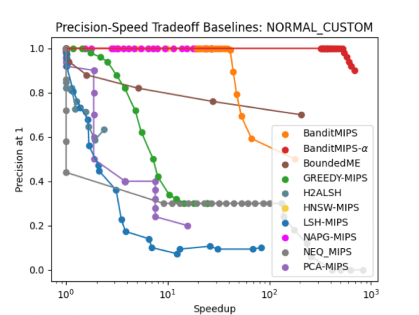
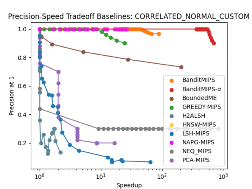
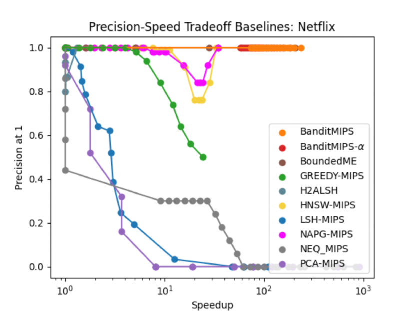
We empirically evaluate the performance of BanditMIPS and the non-uniform sampling version BanditMIPS-$\alpha$ on four synthetic and real-world datasets, comparing them to 8 state-of-art MIPS algorithms. We considered the two synthetic datasets, NORMAL_CUSTOM and CORRELATED_NORMAL_CUSTOM, to assess the performance across a wide parameter range. We further considered the two real-world datasets, the Netflix Prize dataset ($n=6,000$, $d=400,000$) [17] and the Movie Lens dataset ($n=4,000$, $d=6,000$) [45], to provide additional evaluations. We compared our algorithms to 8 baseline MIPS algorithms: LSH-MIPS [84], H2-ALSH-MIPS [48], NEQ-MIPS [31], PCA-MIPS [9], BoundedME [64], Greedy-MIPS [99], HNSW-MIPS [71, 76]. and NAPG-MIPS [91]. Throughout the experiments, we focus on the sample complexity, defined as the number of coordinate-wise multiplications performed. Appendix 9 provides additional details on our experimental settings.

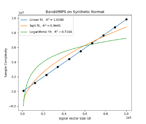
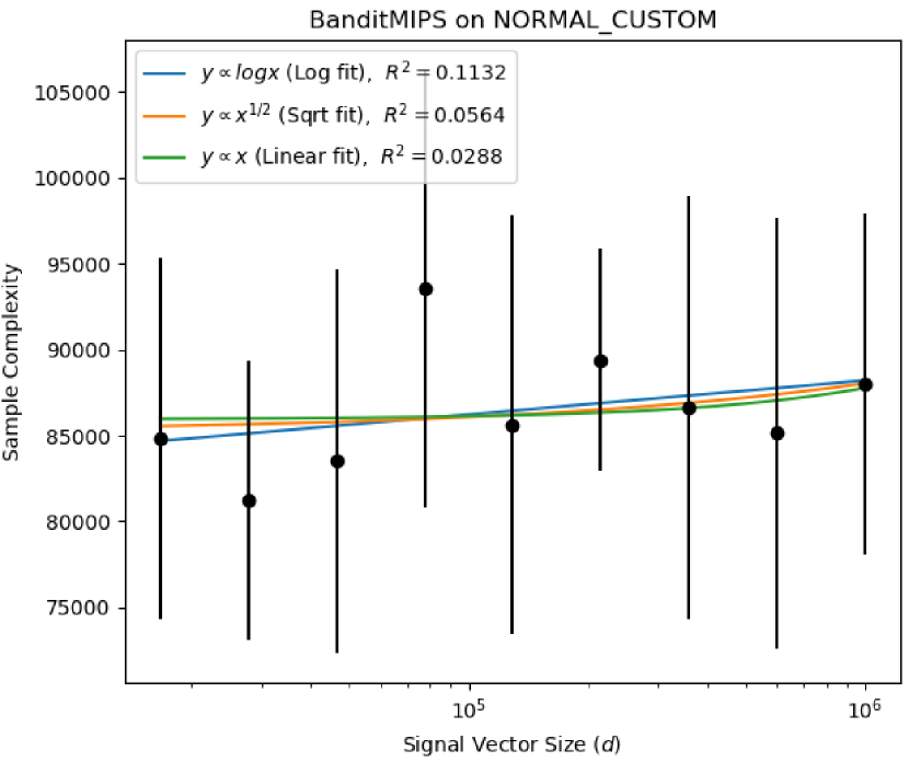
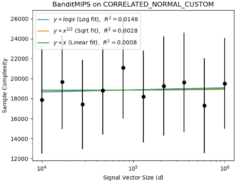
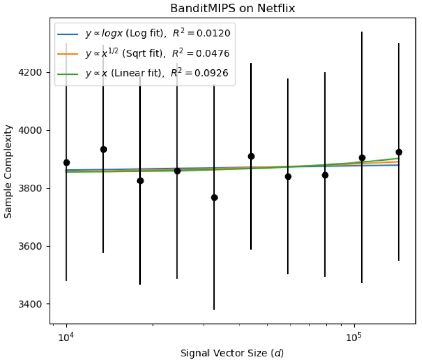
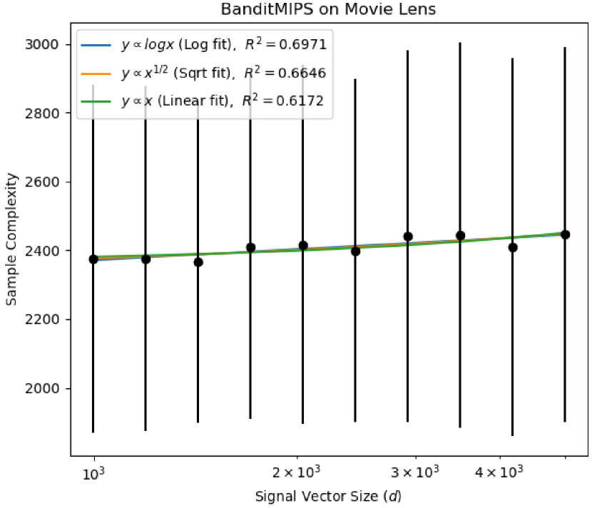
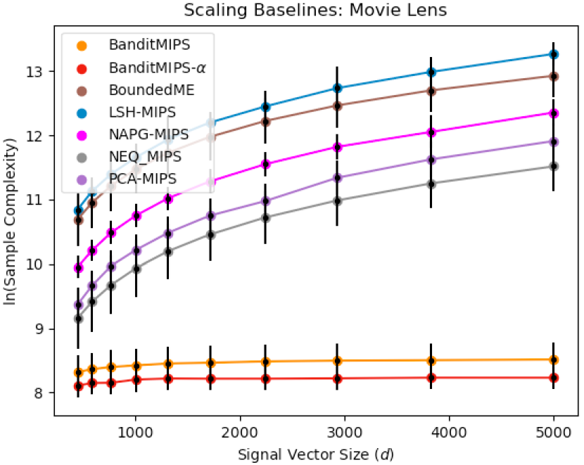
Scaling with $d$: We first assess the scaling with $d$ for BanditMIPS on the four datasets. We subsampled features from the full datasets, evaluating $d$ up to $1,000,000$ on simulated data and up to $400,000$ on real-world data. Results are reported in Figure 1. In all trials, BanditMIPS returns the correct answer to MIPS. We determined that BanditMIPS did not scale with $d$ in all experiments, validating our theoretical results on the sample complexity.

(a)

(b)

(c)

(d)

Figure 1: Sample complexity of BanditMIPS for different values of $d$ on all four datasets. 95% CIs are provided around the mean and are computed from 10 random trials. The sample complexity of BanditMIPS does not scale with $d$. Note that the values of $R^{2}$, the coefficient of determination, are similar for linear, logarithmic, and square root fits, which suggests the scaling is actually constant.

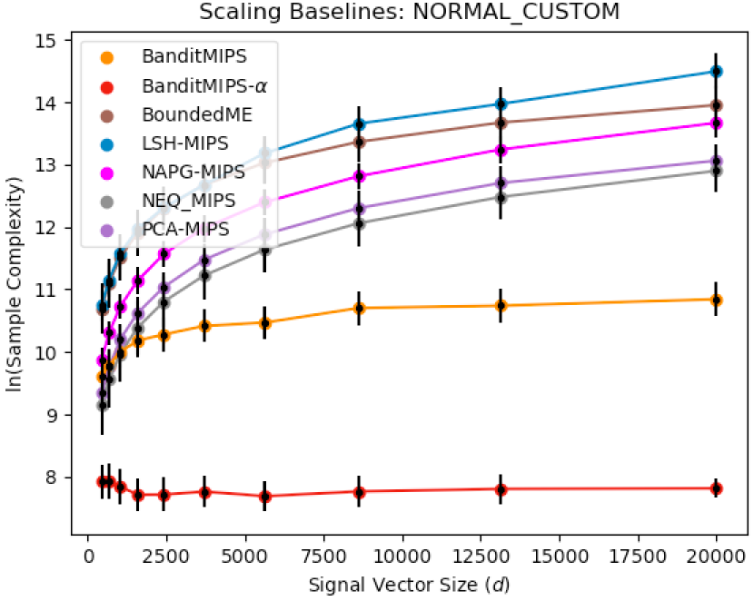
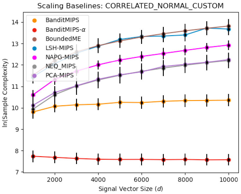
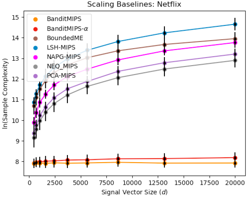
Comparison of sample complexity: We next compare the sample complexity of BanditMIPS and BanditMIPS-$\alpha$ to 8 state-of-art MIPS algorithms on the four datasets across different values of $d$. We only used a subset of up to 20K features because some of the baseline algorithms were prohibitively slow for larger values of $d$. Results are reported in Figure 2. We omit GREEDY-MIPS from Figure 2 because its sample complexity was significantly worse than all algorithms, and omit HNSW-MIPS as its performance was strictly worse than NAPG-MIPS (a related baseline). In measuring sample complexity, we measure query-time sample complexity, i.e., neglect the cost of preprocessing for the baseline algorithms; this is favorable to the baselines. Nonetheless, our two algorithms substantially outperformed other algorithms on all four datasets, demonstrating their superiority in sample efficiency. For example, on the Movie Lens dataset, BanditMIPS and BanditMIPS-$\alpha$ are 20$\times$ and 27$\times$ faster than the closest baseline (NEQ-MIPS). In addition, the non-uniform sampling version BanditMIPS-$\alpha$ outperformed the default version BanditMIPS in 3 out 4 datasets, suggesting the weighted sampling technique further improves sample efficiency. BanditMIPS-$\alpha$ demonstrated slightly worse performance than BanditMIPS on the Netflix dataset, possibly because the highest-value coordinates for the randomly sampled query vectors had low dot products with the atoms.

(a)

(b)

(c)

(d)

Figure 2: Comparison of sample complexity between BanditMIPS, BanditMIPS-$\alpha$, and other baseline algorithms for different values of $d$ across all four datasets. The $y$-axis is on a logarithmic scale. 95% CIs are provided around the mean and are computed from 10 random trials. BanditMIPS and BanditMIPS-$\alpha$ outperformed other baselines.

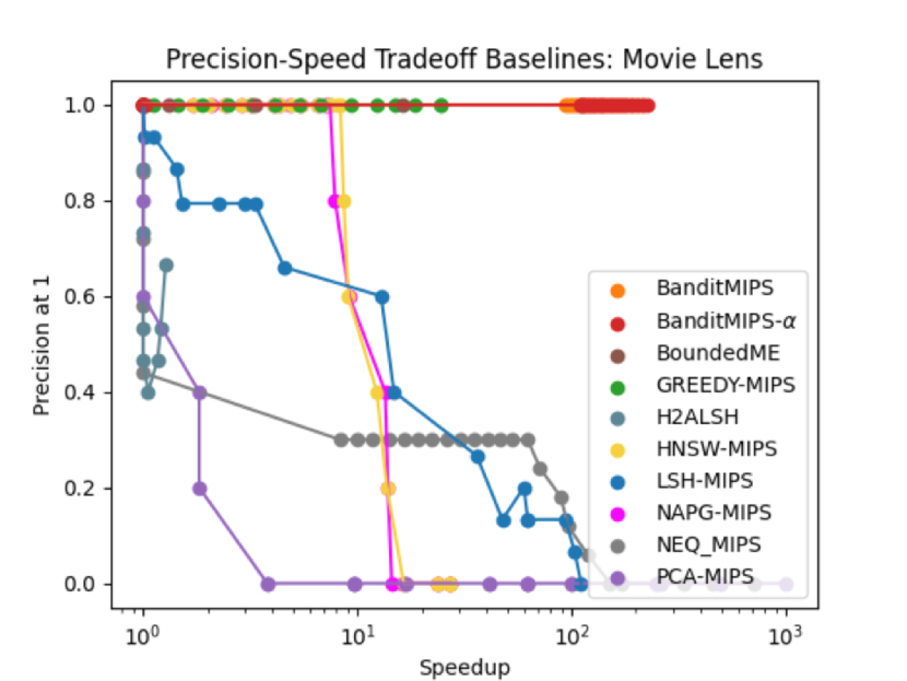
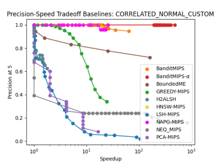
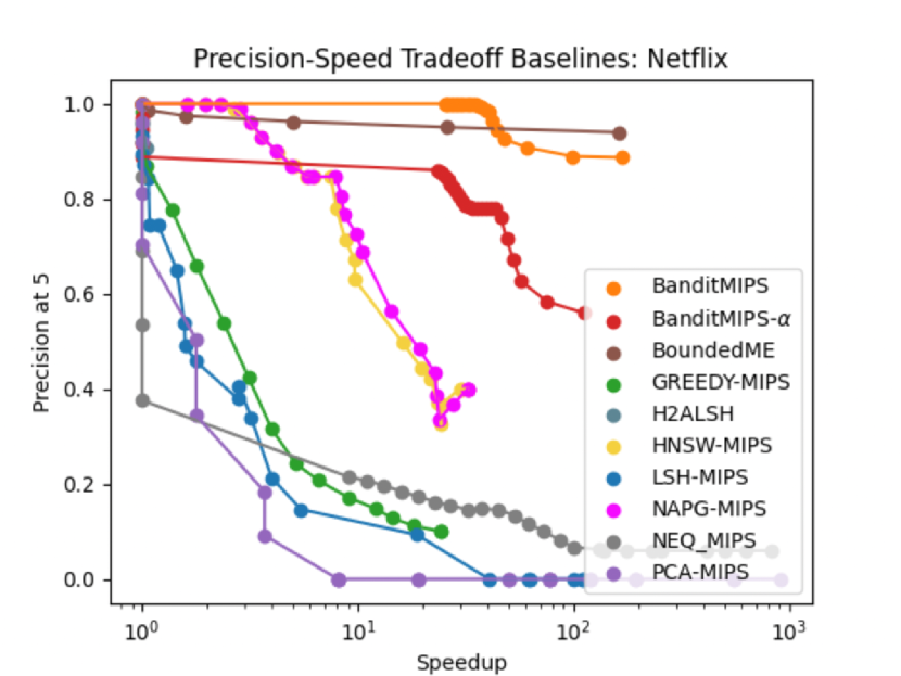
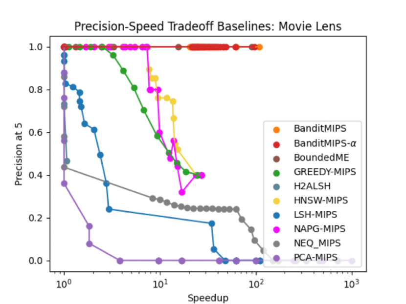
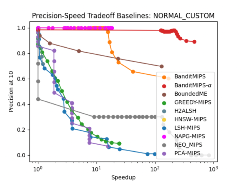
Trade-off between speed and accuracy: Finally, we evaluate the trade-off between speed and accuracy by varying the error probability $\delta$ in our algorithm and the corresponding hyper-parameters in the baseline algorithms (see Appendix 9.3 for more details). As in [64], we define the speedup of an algorithm to be: $\text{speedup}=\frac{\text{sample complexity of na\"{i}ve algorithm}}{\text{sample complexity of compared algorithm}}.$ The accuracy is defined as the proportion of times each algorithm returns the true MIPS solution. Results are reported in Figure 2. Our algorithms achieved the best tradeoff on all four datasets, again demonstrating the superiority of our algorithms in efficiently and accurately solving the MIPS problem. We also considered the $k$-MIPS setting where the goal was to find the top $k$ atoms. Results are reported for $k=5$ and $k=10$ in Appendix 10. Our algorithms obtained a similar improvement over other baselines in these experiments.

(a)

(b)

(c)

(d)

Figure 3: Trade-off between accuracy (equivalent to precision@$1$) and speed for various algorithms across all four datasets. The $x$-axis represents the speedup relative to the naive $O(nd)$ algorithm and the $y$-axis shows the proportion of times an algorithm returned correct answer; higher is better. Each dot represents the mean across 10 random trials and the CIs are omitted for clarity. Our algorithms consistently achieve better accuracies at higher speedup values than the baselines.

(a)

(b)

Figure 4: Sample complexity of BanditMIPS versus $d$ for the Sift-1M and CryptoPairs datasets. BanditMIPS scales as $O(1)$ with respect to $d$ for both datasets. Means and uncertainties were obtained by averaging over 5 random seeds. BanditMIPS returns the correct solution to MIPS in each trial.

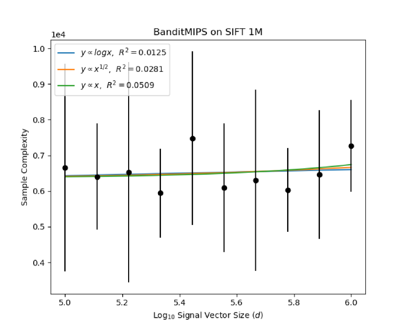
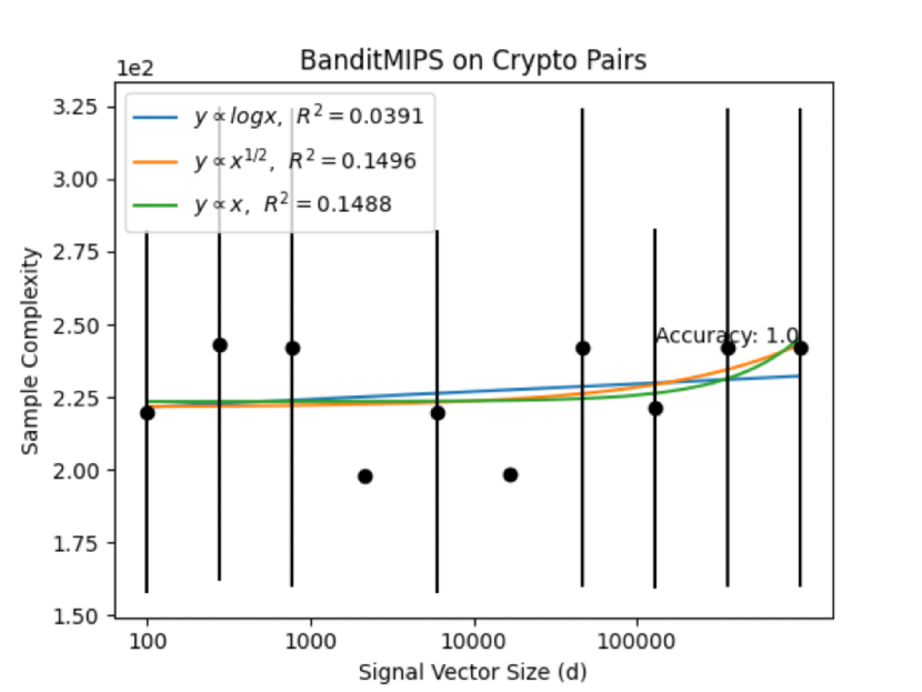
Real-world high-dimensional datasets: We also verify the $O(1)$ scaling with $d$ on two real-world, high-dimensional datasets: the Sift-1M [57] and CryptoPairs datasets [26]. The Sift-1M dataset consists of scale-invariant feature transform [67] features of 128 different images; each image is an atom with $1$ million dimensions. The CryptoPairs dataset consists of the historical trading data of more than 400 trading pairs at 1 minute resolution reaching back until the year 2013. On these datasets, BanditMIPS appears to scale as $O(1)$ with $d$ even to a million dimensions (Figure 4). This suggests that the necessary assumptions outlined in Sections 3.2 and 4 are satisfied on these real-world, high-dimensional datasets. Note that the high dimensionality of these datasets makes them prohibitively expensive to run scaling experiments as in Section 5 or the tradeoff experiments as in Section 2 for baseline algorithms.

6 Conclusions and Limitations

In this work, we presented BanditMIPS and BanditMIPS-$\alpha$, novel algorithms for the MIPS problem. In contrast with prior work, BanditMIPS requires no preprocessing of the data or that the data be nonnegative, and provides hyperparameters to trade off accuracy and runtime. BanditMIPS scales better to high-dimensional datasets under reasonable assumptions and outperformed the prior state-of-the-art significantly. Though the assumptions for BanditMIPS and BanditMIPS-$\alpha$ are often satisfied in practice, requiring them may be a limitation of our approach. In particular, when many of the arm gaps are small, BanditMIPS will compute the inner products for the relevant atoms naïvely.

7 Additional Related Work

In this appendix, we briefly describe other approaches attempt to reduce MIPS to a nearest neighbor search problem (NN). We note that the NN literature is extremely vast and has inspired the use of techniques based on permutation search [78], inverted files [4], vantage-point trees [22], and more. The proliferation of NN algorithms has inspired several associated software packages [18, 56, 21] and tools for practical hyperparameter selection [90]. However, MIPS is fundamentally different from and harder than NN because the inner product is not a proper metric function [76]. Nonetheless, NN techniques have inspired many direct approaches to MIPS, including those that rely on $k$-dimensional or random projection trees [32], concomitants of extreme order statistics [80, 81, 82], ordering permutations [28], principle component analysis (PCA) [9], or hardware acceleration [96, 1]. All of these approaches require significant preprocessing that scales linearly in $d$, e.g., for computing the norms of the query or atom vectors, whereas BanditMIPS does not.

8 Proofs of Theorems

In this appendix, we present the proofs of Theorems 1 and 2.

8.1 Proof of Theorem 1:

Proof.

Following the multi-armed bandit literature, we refer to each index $i$ as an arm and refer to its optimization object $\mu_{i}$ as the arm parameter. We sometimes abuse the terminology and refer to the atom $\mathbf{v}_{i}$ as the arm, with the meaning clear from context. Pulling an arm corresponds to uniformly sampling a coordinate $J$ and evaluating $v_{iJ}q_{J}$ and incurs an $O(1)$ computation. This allows us to focus on the number of arm pulls, which translates directly to coordinate-wise sample complexity.

First, we prove that with probability at least $1-\delta$, all confidence intervals computed throughout the algorithm are valid in that they contain the true parameter $\mu_{i}$’s. For a fixed atom $\mathbf{v}_{i}$ and a given iteration of the algorithm, the $\left(1-\frac{\delta}{2nd_{\text{used}}^{2}}\right)$ confidence interval satisfies

$$\Pr\left(\left|\mu_{i}-\hat{\mu}_{i}\right|>C_{d_{\text{used}}}\right)\leq 2e^{-C_{d_{\text{used}}}^{2}d_{\text{used}}/2\sigma^{2}}\leq\frac{\delta}{2nd_{\text{used}}^{2}}$$

by Hoeffding’s inequality and the choice of $C_{d_{\text{used}}}=\sigma\sqrt{\frac{2\text{log}(4nd^{2}_{\text{used}}/\delta)}{d_{\text{used}}+1}}$. For a fixed arm $i$, for any value of $d_{\text{used}}$ we have that the confidence interval is correct with probability at least $1-\frac{\delta}{n}$, where we used the fact that $1+\frac{1}{2^{2}}+\frac{1}{3^{2}}+\ldots=\frac{\pi^{2}}{6}<2$. By another union bound over all $n$ arm indices, all confidence intervals constructed by the algorithm are correct with probability at least $1-\delta$.

Next, we prove the correctness of BanditMIPS. Let $i^{*}=\operatorname*{arg\,max}_{i\in[n]}\mu_{i}$ be the desired output of the algorithm. First, observe that the main while loop in the algorithm can only run $d$ times, so the algorithm must terminate. Furthermore, if all confidence intervals throughout the algorithm are valid, which is the case with probability at least $1-\delta$, $i^{*}$ cannot be removed from the set of candidate arms. Hence, $\mathbf{v}_{i^{*}}$ (or some $\mathbf{v}_{i}$ with $\mu_{i}=\mu_{i^{*}}$) must be returned upon termination with probability at least $1-\delta$. This proves the correctness of Algorithm 1.

Finally, we examine the complexity of BanditMIPS. Let $d_{\text{used}}$ be the total number of arm pulls computed for each of the arms remaining in the set of candidate arms at a given iteration in the algorithm. Note that for any suboptimal arm $i\neq i^{*}$ that has not left the set of candidate arms $\mathcal{S}_{\text{solution}}$, we must have $C_{d_{\text{used}}}\leq c_{0}\sqrt{\frac{\log(1/\delta)}{d_{\text{used}}}}$ by assumption (and this holds for our specific choice of $C_{d_{\text{used}}}$ in Algorithm 1). With $\Delta_{i}=\mu_{i^{*}}-\mu_{i}$, if $d_{\text{used}}>\frac{16c_{0}^{2}}{\Delta_{i}^{2}}\log\frac{n}{\delta\Delta_{i}}$, then

$$4C_{d_{\text{used}}} \leq 4c_{0}\sqrt{\frac{{\log\frac{n}{\delta\Delta_{i}}}}{{d_{\text{used}}}}}<\Delta_{i}$$

Furthermore,

$$\hat{\mu}_{i^{*}}-C_{d_{\text{used}}} \geq\mu_{i^{*}}-2C_{d_{\text{used}}}$$

$$=\mu_{i}+\Delta_{i}-2C_{d_{\text{used}}}$$

$$>\mu_{i}+2C_{d_{\text{used}}}$$

$$>\hat{\mu}_{i}+C_{d_{\text{used}}}$$

which means that $i$ must be removed from the set of candidate arms by the end of that iteration.

Hence, the number of data point computations $M_{i}$ required for any arm $i\neq i^{*}$ is at most

$$M_{i}\leq\min\left[\frac{16c_{0}^{2}}{\Delta_{i}^{2}}\log\frac{n}{\delta\Delta_{i}}+1,2d\right]$$

where we used the fact that the maximum number of computations for any arm is $2d$ when sampling with replacement. Note that bound this holds simultaneously for all arms $i$ with probability at least $1-\delta$. We conclude that the total number of arm pulls $M$ satisfies

$$M \leq\sum_{i\in[n]}\min\left[\frac{16c_{0}^{2}}{\Delta_{i}^{2}}\log\frac{n}{\delta\Delta_{i}}+1,2d\right]$$

with probability at least $1-\delta$.

As argued before, since each arm pull involves an $O(1)$ computation, $M$ also corresponds to the total number of operations up to a constant factor. ∎

8.2 Proof of Theorem 2

Proof.

Since all the $X_{iJ}$’s are unbiased, optimizing Problem (3) is equivalent to minimizing the combined second moment

$$\sum_{i\in[n]}\mathbb{E}_{J\sim P_{\mathbf{w}}}[X_{iJ}^{2}] =\sum_{i\in[n]}\sum_{j\in[d]}\frac{1}{d^{2}w_{j}}q_{j}^{2}v_{ij}^{2}$$ (5)

$$=\sum_{j\in[d]}\left(\frac{1}{d^{2}w_{j}}q_{j}^{2}\sum_{i\in[n]}v_{ij}^{2}\right).$$ (6)

The Lagrangian is given by

$$\mathcal{L}(\mathbf{w},\nu)=\sum_{j\in[d]}\left(\frac{1}{d^{2}w_{j}}q_{j}^{2}\sum_{i\in[n]}v_{ij}^{2}\right)+\nu\left(1-\sum_{j\in[d]}w_{j}\right).$$ (7)

Furthermore, the derivatives are

$$\frac{\partial\mathcal{L}(\mathbf{w},\nu)}{\partial w_{j}}=-\frac{q_{j}^{2}\sum_{i\in[n]}v_{ij}^{2}}{d^{2}w_{j}^{2}}-\nu$$ (8)

$$\frac{\partial\mathcal{L}(\mathbf{w},\nu)}{\partial\mu}=1-\sum_{j\in[d]}w_{j}.$$ (9)

By the Karush-Kuhn-Tucker (KKT) conditions, setting the derivatives to 0 gives

$$w_{j}^{*}=\frac{\sqrt{q_{j}^{2}\sum_{i\in[n]}v_{ij}^{2}}}{\sum_{j\in[d]}\sqrt{q_{j}^{2}\sum_{i\in[n]}v_{ij}^{2}}}~{}~{}~{}~{}\text{ for }~{}j=1,\ldots,d.$$ (10)

∎

9 Description of Datasets

Here, we provide a more detailed description of the datasets used in our experiments.

9.1 Synthetic Datasets

In the NORMAL_CUSTOM dataset, a parameter $\theta_{i}$ is drawn for each atom from a standard normal distribution, then each coordinate for that atom is drawn from $\mathcal{N}(\theta_{i},1)$. The signals are generated similarly.

In the CORRELATED_NORMAL_CUSTOM dataset, a parameter $\theta$ is for the signal $\mathbf{q}$ from a standard normal distribution, then each coordinate for that signal is drawn from $\mathcal{N}(\theta,1)$. Atom $\mathbf{v}_{i}$ is generated by first sampling a random weight $w_{i}\sim\mathcal{N}(0,1)$; then atom $\mathbf{v}_{i}$ is set to $w_{i}\mathbf{q}$ plus Gaussian noise.

Note that for the synthetic datasets, we can vary $n$ and $d$. The values of $n$ and $d$ chosen for each experiment are described in Subsection 9.3.

9.2 Real-world datasets

Netflix Dataset: We use a subset of the data from the Netflix Prize dataset [17] that contains the ratings of 6,000 movies by 400,000 customers. We impute missing ratings by approximating the data matrix via a low-rank approximation. Specifically, we approximate the data matrix via a 100-factor SVD decomposition. The movie vectors are used as the query vectors and atoms and $d$ corresponds to the number of subsampled users.

Movie Lens Dataset: We use Movie Lens-1M dataset [45], which consists of 1 million ratings of 4,000 movies by 6,000 users. As for the Netflix dataset, we impute missing ratings by obtaining a low-rank approximation to the data matrix. Specifically, we perform apply a Non-negative Matrix Factorization (NMF) with 15 factors to the dataset to impute missing values. The movie vectors are used as the query vectors and atoms, with $d$ corresponding to the number of subsampled users.

We note that for all datasets, the coordinate-wise inner products are sub-Gaussian random variables. In particular, this means the assumptions of Theorem 1 are satisfied and we can construct confidence intervals that scale as $O\left(\sqrt{\frac{\log 1/\delta^{\prime}}{d^{\prime}}}\right)$. We describe the setting for the sub-Gaussianity parameters in Section 9.3.

9.3 Experimental Settings

Scaling Experiments: In all scaling experiments, $\delta$ and $\epsilon$ were both set to $0.001$ for BanditMIPS and BanditMIPS-$\alpha$. For the NORMAL_CUSTOM and CORRELATED_NORMAL_CUSTOM datasets, the sub-Gaussianity parameter was set to $1$. For the Netflix and Movie Lens datasets, the sub-Gaussianity parameter was set to $25$. For the CryptoPairs, SIFT-1M, and SimpleSong datasets described in Appendix 12, the sub-Gaussianity parameters were set to $2.5e9$, $6.25e5$, and $25$, respectively. The number of atoms was set to $100$ and all other atoms used default values of hyperparameters for their sub-Gaussianity parameters.

Tradeoff Experiments: For the tradeoff experiments, the number of dimensions was fixed to $d=10,000$. The various values of speedups were obtained by varying the hyperparameters of each algorithm. For NAPG-MIPS and HNSW-MIPS, for example, $M$ was varied from 4 to 32, $ef\_constructions$ was varied from $2$ to $500$, and $ef\_searches$ was varied from $2$ to $500$. For Greedy-MIPS, $budget$ varied from 2 to 999. For LSH-MIPS, the number of hash functions and hash values vary from 1 to 10. For H2ALSH, $\delta$ varies from $\frac{1}{2^{4}}$ to $\frac{1}{2}$, $c_{0}$ varies from 1.2 to 5, and $c$ varies from 0.9 to 2. For NEQ-MIPS, the number of codewords and codebooks vary from 1 to 100. For BanditMIPS , BanditMIPS-$\alpha$, and BoundedME, speedups were obtained by varying $\delta$ from $\frac{1}{10^{10}}$ to $0.99$ and $\epsilon$ from $\frac{1}{10^{10}}$ to $3$. In our code submission, we include a one-line script to reproduce all of our results and plots.

All experiments were run on a 2019 Macbook Pro with a 2.4 GHz 8-Core Intel Core i9 CPU, 64 GB 2667 MHz DDR4 RAM, and an Intel UHD Graphics 630 1536 MB graphics card. Our results, however, should not be sensitive to hardware, as we used hardware-independent performance metrics (the number of coordinate-wise multiplications) for our results.

10 Additional Experimental Results

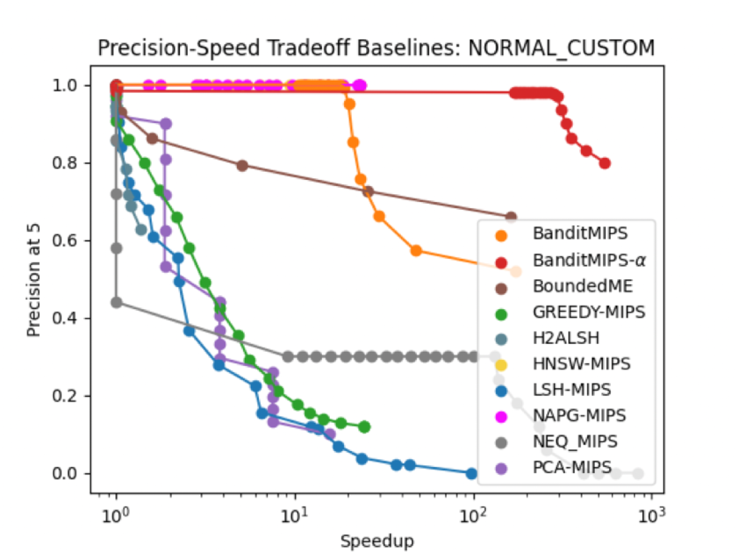
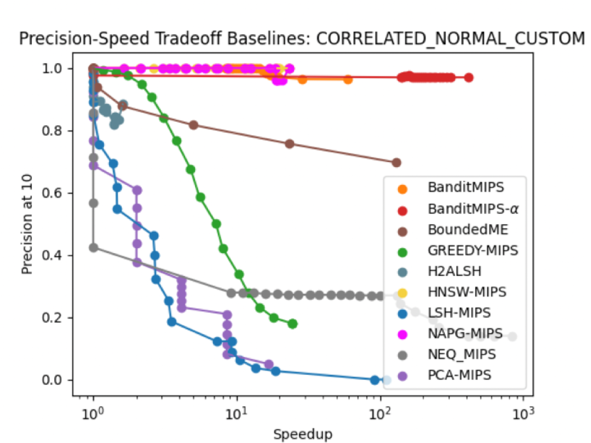
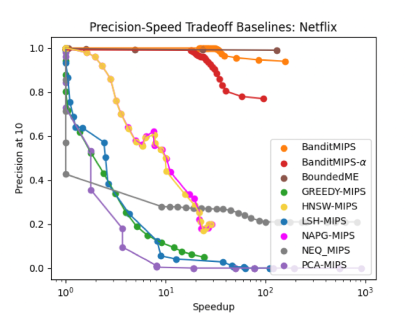
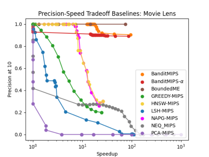
Here, we present the results for precision@$k$ versus algorithm speedup for various algorithms for $k=5$ and $10$; see Figures 5 and 6. The precision@$k$ is defined as the proportion of true top $k$ atoms surfaced in the algorithm’s returned top $k$ atoms (the precision@$k$ is also the top-$k$ accuracy, i.e., the proportion of correctly identified top $k$ atoms).

(a)

(b)

(c)

(d)

Figure 5: Trade-off between top-$5$ accuracy (precision@$5$) and speed for various algorithms across all four datasets. The $x$-axis represents the speedup relative to the naive $O(nd)$ algorithm and the $y$-axis shows the proportion of times an algorithm returned correct answer; higher is better. Each dot represents the mean across 10 random trials and the CIs are omitted for clarity. Our algorithms consistently achieve better accuracies at higher speedup values than the baselines.

(a)

(b)

(c)

(d)

Figure 6: Trade-off between top-$10$ accuracy (precision@$10$) and speed for various algorithms across all four datasets. The $x$-axis represents the speedup relative to the naive $O(nd)$ algorithm and the $y$-axis shows the proportion of times an algorithm returned correct answer; higher is better. Each dot represents the mean across 10 random trials and the CIs are omitted for clarity. Our algorithms consistently achieve better accuracies at higher speedup values than the baselines.

11 Using Preprocessing Techniques with BanditMIPS

In this Appendix, we discuss using preprocessing techniques with BanditMIPS. The specific form of preprocessing is binning by estimated norm. More precisely, we estimate the norm of each atom by sampling a constant number of coordinates from them. We then sort the atoms by estimated norm into bins, where each bin contains $k=30$ atoms (note that $k$ is a hyperparameter). The top $k$ atoms with the highest estimated norm are sorted into the first bin, the next $k$ atoms are sorted into the second bin, and so on.

When running BanditMIPS, we find the best atom in each bin but stop sampling an atom if the best atom we have found across all bins has a sampled inner product greater than another atom’s maximum potential inner product. Intuitively, this allows us to filter atoms with small estimated norm more quickly if an atom in another bin is very likely to be a better candidate.

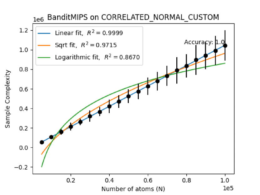
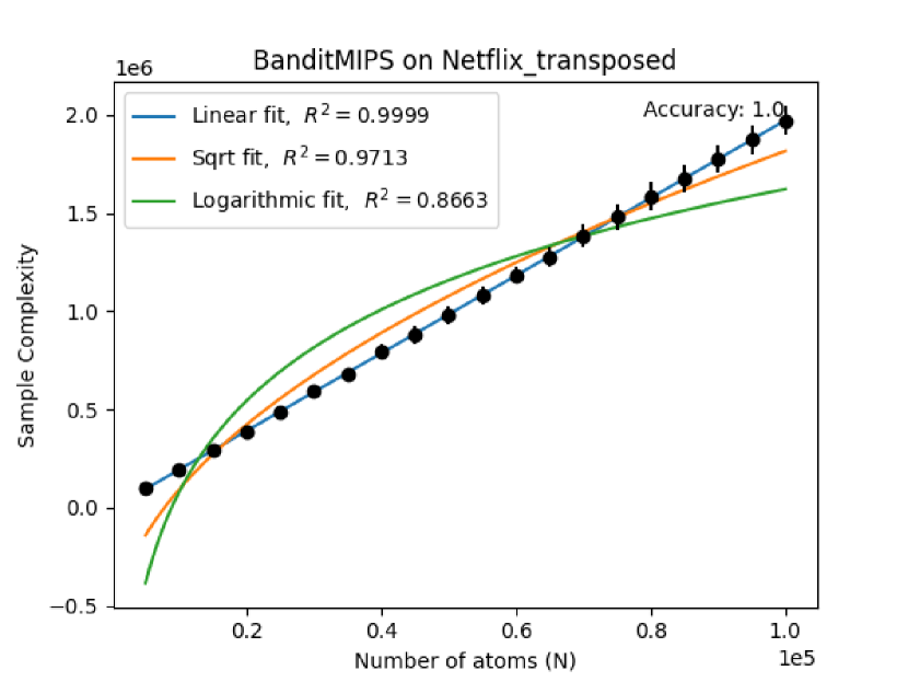
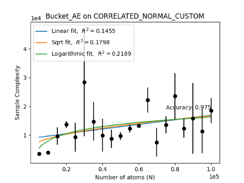
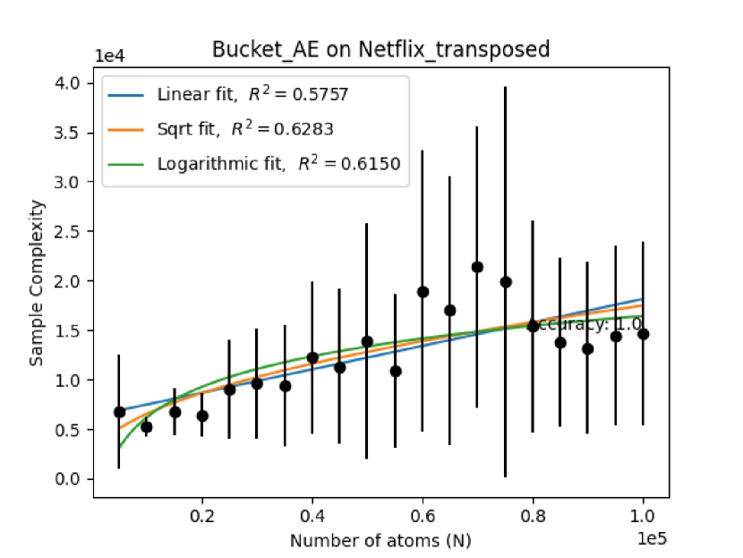
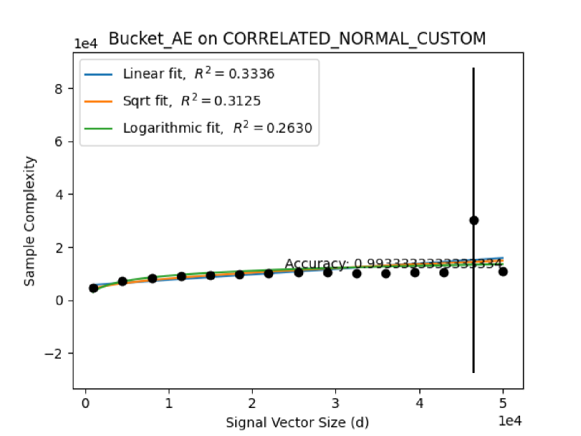
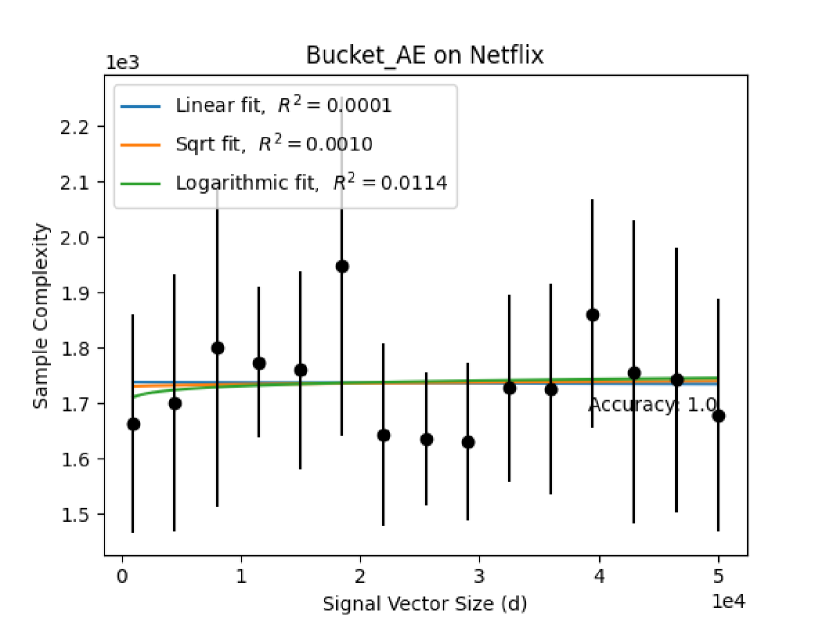
We call this algorithm (BanditMIPS with this form of preprocessing) Bucket_AE. Figure 7 demonstrates that Bucket_AE reduces the scaling with $n$ of BanditMIPS. Furthermore, Bucket_AE still scales as $O(1)$ with $d$.

We leave an exact complexity analysis of this preprocessing’s affect on the scaling with $n$ under various distributional assumptions to future work.

(a)

(b)

(c)

(d)

(e)

(f)

Figure 7: Top left and top right: sample complexity of BanditMIPS versus $n$ for the CORRELATED_NORMAL_CUSTOM and Netflix datasets. BanditMIPS scales linearly with $n$. Middle left and middle right: BanditMIPS with preprocessing Bucket_AE scales sublinearly with $n$. This suggests that the form of preprocessing we apply is useful for reducing the complexity of our algorithm with $n$. Bottom left and bottom right: Bucket_AE still scales as $O(1)$ with $d$. Means and uncertainties were obtained from 10 random seeds.

12 Experiments High Dimensional Datasets and Application to Matching Pursuit

One of the advantages of BanditMIPS is that it has no dependence on dataset dimensionality when the necessary assumptions are satisfied. We also demonstrate the $O(1)$ scaling with $d$ of BanditMIPS explicitly on a high-dimensional synthetic dataset and discuss an application to the Matching Pursuit problem (MP).

12.1 Application to Matching Pursuit in High Dimensions: the SimpleSong Dataset

12.1.1 Description of the SimpleSong Dataset

We construct a simple synthetic dataset, entitled the SimpleSong Dataset. In this dataset, the query and atoms are audio signals sampled at 44,100 Hz and each coordinate value represents the signal’s amplitude at a given point in time. Common musical notes are represented as periodic sine waves with the frequencies given in Table 2.

Table 2: Frequencies for various musical notes.

Note	Frequency (Hz)
C4	256
E4	330
G4	392
C5	512
E5	660
G5	784

The query in this dataset is a simple song. The song is structured in 1 minute intervals, where the first interval – called an A interval – consists of a C4-E4-G4 chord and the second interval – called a B interval – consists of a G4-C5-E5 chord. The song is then repeated $t$ times, bringing its total length to $2t$ minutes. The dimensionality of the the signal is $d=2t*44,100=88,200t$. The weights of the C4, E4, and G4 waves in the A intervals and the G4, C5, and E5 waves in the B intervals are in the ratio 1:2:3:3:2.5:1.5.

The atoms in this dataset are the sine waves corresponding to the notes with the frequencies show in Table 2, as well as notes of other frequencies.

12.1.2 Matching Pursuit and Fourier Transforms

The Matching Pursuit problem (MP) is a problem in which a vector $\mathbf{q}$ is approximated as a linear combination of the atoms $\mathbf{v}_{1},\ldots,\mathbf{v}_{n}$. A common algorithm for MP involves solving MIPS to find the atom $\mathbf{v}_{i^{*}}$ with the highest inner product with the query, subtracting the component of the query parallel to $\mathbf{v}_{i^{*}}$, and re-iterating this process with the residual. Such an approach solves MIPS several times as a subroutine. Thus, an algorithm which accelerates MIPS should also then accelerate MP.

In the audio domain, we note that when the atoms $\mathbf{v}_{1},\ldots,\mathbf{v}_{n}$ are periodic functions with predefined frequencies, MP becomes a form of Fourier analysis in which the atoms are the Fourier components and their inner products with the query correspond to Fourier coefficients. For more detailed background on Fourier theory, we refer the reader to [24].

12.1.3 Experimental Results

For convenience, we restrict $t$ to be an integer in our experiments so a whole number of AB intervals are completed. We ran BanditMIPS with $\delta=\frac{1}{10,000}$ and $\sigma^{2}=6.25$ over $3$ random seeds for various values of $t$.

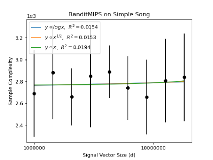
BanditMIPS is correctly able to recover the notes played in the song in order of decreasing strength: G4, C5, E4, E5, and C4 in each experiment. Furthermore, BanditMIPS is able to calculate their Fourier coefficients correctly. Crucially, the complexity of BanditMIPS to identify these components does not scale with $d$, the length of the song. Figure 8 demonstrates the total sample complexity of BanditMIPS to identify the first five Fourier components (five iterations of MIPS) of the song as the song length increases.

Figure 8: Sample complexity of MP when using BanditMIPS as a subroutine for MIPS on the SimpleSong dataset. The complexity of the solving the problem does not scale with the length of the song, $d$. Uncertainties and means were obtained from 3 random seeds. BanditMIPS returns the correct solution to MIPS in each trial.

Our approach may suggest an application to Fourier transforms, which aim to represent signals in terms of constituent signals with predetermined set of frequencies. We acknowledge, however, that Fourier analysis is a well-developed field and that further research is necessary to compare such a method to state-of-the-art Fourier transform methods, which may already be heavily optimized or sampling-based.

13 BanditMIPS on a Highly Symmetric Dataset

In this section, we discuss a dataset on which the assumptions in Section 4 fail, namely when $\Delta$ scales with $d$. In this setting, BanditMIPS does not scale as $O(1)$ and instead scales linearly with $d$, as is expected.

We call this dataset the SymmetricNormal dataset. In this dataset, the signal has each coordinate drawn from $\mathcal{N}(0,1)$ and each atom’s coordinate is drawn i.i.d. from $\mathcal{N}(0,1)$. Note that all atoms are therefore symmetric a priori.

We now consider the quantity $\Delta_{i,j}(d)\coloneqq\mu_{1}(d)-\mu_{2}(d)$, i.e., the gap between the first and second arm, where our notation emphasizes we are studying each quantity as $d$ increases. Note that $\Delta_{i,j}(d)=\frac{\mathbf{v}_{1}^{T}q-\mathbf{v}_{2}^{T}q}{d}$. By the Central Limit Theorem, the sequence of random variables $\sqrt{d}\Delta_{i,j}(d)$ converges in distribution to $\mathcal{N}(0,\sigma^{2}_{i,j})$ for some constant $\sigma^{2}_{i,j}$. Crucially, this implies that $\Delta_{i,j}(d)$ is on the order of $\frac{1}{\sqrt{d}}$.

The complexity result from Theorem 1 then predicts that BanditMIPS scales linearly with $d$. Indeed, this is what we observe in Figure 9.

Figure 9: Sample complexity of BanditMIPS on the SymmetricNormal dataset. The sample complexity of BanditMIPS is linear with $d$, as is expected. Uncertainties and means were obtained from 10 random seeds.

References

- [1] Firas Abuzaid, Geet Sethi, Peter Bailis, and Matei Zaharia. To Index or Not to Index: Optimizing Exact Maximum Inner Product Search. In 2019 IEEE 35th International Conference on Data Engineering (ICDE), pages 1250–1261, April 2019. ISSN: 2375-026X.
- [2] P. Alexander, Yury Malkov, L. Andrey, and V. Krylov. Approximate Nearest Neighbor Search Small World Approach. 2011.
- [3] Daichi Amagata and Takahiro Hara. Reverse Maximum Inner Product Search: How to efficiently find users who would like to buy my item? Fifteenth ACM Conference on Recommender Systems, pages 273–281, September 2021. Conference Name: RecSys ’21: Fifteenth ACM Conference on Recommender Systems ISBN: 9781450384582 Place: Amsterdam Netherlands Publisher: ACM.
- [4] Giuseppe Amato and Pasquale Savino. Approximate similarity search in metric spaces using inverted files. In Ronny Lempel, Raffaele Perego, and Fabrizio Silvestri, editors, 3rd International ICST Conference on Scalable Information Systems, INFOSCALE 2008, Vico Equense, Italy, June 4-6, 2008, page 28. ICST / ACM, 2008.
- [5] Alexandr Andoni, Piotr Indyk, Thijs Laarhoven, Ilya Razenshteyn, and Ludwig Schmidt. Practical and optimal LSH for angular distance. In C. Cortes, N. Lawrence, D. Lee, M. Sugiyama, and R. Garnett, editors, Advances in neural information processing systems, volume 28. Curran Associates, Inc., 2015.
- [6] Imad Aouali, Amine Benhalloum, Martin Bompaire, Achraf Ait Sidi Hammou, Sergey Ivanov, Benjamin Heymann, David Rohde, Otmane Sakhi, Flavian Vasile, and Maxime Vono. Reward Optimizing Recommendation using Deep Learning and Fast Maximum Inner Product Search. In Proceedings of the 28th ACM SIGKDD Conference on Knowledge Discovery and Data Mining, KDD ’22, pages 4772–4773, New York, NY, USA, August 2022. Association for Computing Machinery.
- [7] Jean-yves Audibert, Sébastien Bubeck, and Rémi Munos. Best arm identification in multiarmed bandits. In In 23rd Annual Conference on Learning Theory, 2010.
- [8] Artem Babenko and Victor Lempitsky. The inverted multi-index. In 2012 IEEE Conference on Computer Vision and Pattern Recognition, pages 3069–3076, June 2012. ISSN: 1063-6919.
- [9] Yoram Bachrach, Yehuda Finkelstein, Ran Gilad-Bachrach, Liran Katzir, Noam Koenigstein, Nir Nice, and Ulrich Paquet. Speeding up the Xbox recommender system using a euclidean transformation for inner-product spaces. In Proceedings of the 8th ACM Conference on Recommender Systems, RecSys ’14, pages 257–264, New York, NY, USA, October 2014. Association for Computing Machinery.
- [10] Vivek Bagaria, Tavor Z Baharav, Govinda M Kamath, and N Tse David. Bandit-based monte carlo optimization for nearest neighbors. IEEE Journal on Selected Areas in Information Theory, 2(2):599–610, 2021.
- [11] Vivek Bagaria, Govinda M. Kamath, Vasilis Ntranos, Martin J. Zhang, and David Tse. Medoids in almost-linear time via multi-armed bandits. In International Conference on Artificial Intelligence and Statistics, pages 500–509, 2018.
- [12] Vivek Bagaria, Govinda M. Kamath, and David Tse. Adaptive monte-carlo optimization. arXiv:1805.08321, 2018.
- [13] Tavor Z Baharav, Gary Cheng, Mert Pilanci, and David Tse. Approximate function evaluation via multi-armed bandits. In International Conference on Artificial Intelligence and Statistics, pages 108–135. PMLR, 2022.
- [14] Tavor Z. Baharav and David Tse. Ultra fast medoid identification via correlated sequential halving. In Advances in Neural Information Processing Systems, pages 3650–3659, 2019.
- [15] Grey Ballard, Tamara G. Kolda, Ali Pinar, and C. Seshadhri. Diamond Sampling for Approximate Maximum All-Pairs Dot-Product (MAD) Search. In 2015 IEEE International Conference on Data Mining, pages 11–20, Atlantic City, NJ, USA, November 2015. IEEE.
- [16] Rémi Bardenet and Odalric-Ambrym Maillard. Concentration inequalities for sampling without replacement. Bernoulli, 21(3):1361–1385, August 2015.
- [17] James Bennett, Stan Lanning, and Netflix Netflix. The Netflix Prize. In In KDD Cup and Workshop in Conjunction with KDD, 2007.
- [18] Erik Bernhardsson. Annoy: Approximate Nearest Neighbors in C++/Python, 2018. Python package version 1.13.0.
- [19] Sebastian Borgeaud, Arthur Mensch, Jordan Hoffmann, Trevor Cai, Eliza Rutherford, Katie Millican, George Bm Van Den Driessche, Jean-Baptiste Lespiau, Bogdan Damoc, Aidan Clark, Diego De Las Casas, Aurelia Guy, Jacob Menick, Roman Ring, Tom Hennigan, Saffron Huang, Loren Maggiore, Chris Jones, Albin Cassirer, Andy Brock, Michela Paganini, Geoffrey Irving, Oriol Vinyals, Simon Osindero, Karen Simonyan, Jack Rae, Erich Elsen, and Laurent Sifre. Improving Language Models by Retrieving from Trillions of Tokens. In Proceedings of the 39th International Conference on Machine Learning, pages 2206–2240. PMLR, June 2022.
- [20] Stéphane Boucheron, Gábor Lugosi, and Pascal Massart. Concentration Inequalities: A Nonasymptotic Theory of Independence. February 2013.
- [21] Leonid Boytsov and Bilegsaikhan Naidan. Engineering efficient and effective non-metric space library. In Nieves R. Brisaboa, Oscar Pedreira, and Pavel Zezula, editors, Similarity Search and Applications - 6th International Conference, SISAP 2013, A Coruña, Spain, October 2-4, 2013, Proceedings, volume 8199 of Lecture Notes in Computer Science, pages 280–293. Springer, 2013.
- [22] Leonid Boytsov and Bilegsaikhan Naidan. Learning to prune in metric and non-metric spaces. In Christopher J. C. Burges, Léon Bottou, Zoubin Ghahramani, and Kilian Q. Weinberger, editors, Advances in Neural Information Processing Systems 26: 27th Annual Conference on Neural Information Processing Systems 2013. Proceedings of a meeting held December 5-8, 2013, Lake Tahoe, Nevada, United States, pages 1574–1582, 2013.
- [23] Leonid Boytsov, David Novak, Yury A. Malkov, and Eric Nyberg. Off the beaten path: Let’s replace term-based retrieval with k-nn search. In Snehasis Mukhopadhyay, ChengXiang Zhai, Elisa Bertino, Fabio Crestani, Javed Mostafa, Jie Tang, Luo Si, Xiaofang Zhou, Yi Chang, Yunyao Li, and Parikshit Sondhi, editors, Proceedings of the 25th ACM International Conference on Information and Knowledge Management, CIKM 2016, Indianapolis, IN, USA, October 24-28, 2016, pages 1099–1108. ACM, 2016.
- [24] E. Oran Brigham. The Fast Fourier Transform and Its Applications. 1988.
- [25] Sébastien Bubeck, Rémi Munos, and Gilles Stoltz. Pure exploration in finitely-armed and continuous-armed bandits. Theoretical Computer Science, 412(19):1832–1852, April 2011.
- [26] Carsten. 400+ crypto currency pairs at 1-minute resolution, 2022.
- [27] Olivier Catoni. Challenging the empirical mean and empirical variance: a deviation study. In Annales de l’IHP Probabilités et statistiques, volume 48, pages 1148–1185, 2012.
- [28] Edgar Chávez, Karina Figueroa, and Gonzalo Navarro. Effective proximity retrieval by ordering permutations. IEEE Trans. Pattern Anal. Mach. Intell., 30(9):1647–1658, 2008.
- [29] Patrick H. Chen, Chang Wei-cheng, Yu Hsiang-fu, Inderjit S. Dhillon, and Hsieh Cho-jui. FINGER: Fast Inference for Graph-based Approximate Nearest Neighbor Search, June 2022. arXiv:2206.11408 [cs].
- [30] Paolo Cremonesi, Yehuda Koren, and Roberto Turrin. Performance of recommender algorithms on top-n recommendation tasks. In Proceedings of the fourth ACM conference on Recommender systems, pages 39–46, 2010.
- [31] Xinyan Dai, Xiao Yan, Kelvin K. W. Ng, Jiu Liu, and James Cheng. Norm-Explicit Quantization: Improving Vector Quantization for Maximum Inner Product Search. In Proceedings of the AAAI Conference on Artificial Intelligence, volume 34, pages 51–58, April 2020. ISSN: 2374-3468, 2159-5399 Issue: 01 Journal Abbreviation: AAAI.
- [32] Sanjoy Dasgupta. Random projection trees and low dimensional manifolds. pages 537–546, May 2008.
- [33] Thomas Dean, Mark A. Ruzon, Mark Segal, Jonathon Shlens, Sudheendra Vijayanarasimhan, and Jay Yagnik. Fast, Accurate Detection of 100,000 Object Classes on a Single Machine. In 2013 IEEE Conference on Computer Vision and Pattern Recognition, pages 1814–1821, Portland, OR, USA, June 2013. IEEE.
- [34] Qin Ding, Hsiang-Fu Yu, and Cho-Jui Hsieh. A Fast Sampling Algorithm for Maximum Inner Product Search. In Proceedings of the Twenty-Second International Conference on Artificial Intelligence and Statistics, pages 3004–3012. PMLR, April 2019. ISSN: 2640-3498.
- [35] Wei Dong, Zhe Wang, Moses Charikar, and Kai Li. High-confidence near-duplicate image detection. In Horace Ho-Shing Ip and Yong Rui, editors, International Conference on Multimedia Retrieval, ICMR ’12, Hong Kong, China, June 5-8, 2012, page 1. ACM, 2012.
- [36] David L. Donoho, Yaakov Tsaig, Iddo Drori, and Jean-Luc Starck. Sparse Solution of Underdetermined Systems of Linear Equations by Stagewise Orthogonal Matching Pursuit. IEEE Transactions on Information Theory, 58(2):1094–1121, February 2012.
- [37] Matthijs Douze, Hervé Jégou, and Florent Perronnin. Polysemous Codes. In Bastian Leibe, Jiri Matas, Nicu Sebe, and Max Welling, editors, Computer Vision – ECCV 2016, Lecture Notes in Computer Science, pages 785–801, Cham, 2016. Springer International Publishing.
- [38] Eyal Even-Dar, Shie Mannor, and Yishay Mansour. PAC Bounds for Multi-armed Bandit and Markov Decision Processes. In Jyrki Kivinen and Robert H. Sloan, editors, Computational Learning Theory, Lecture Notes in Computer Science, pages 255–270, Berlin, Heidelberg, 2002. Springer.
- [39] Eyal Even-Dar, Shie Mannor, and Yishay Mansour. Action Elimination and Stopping Conditions for the Multi-Armed Bandit and Reinforcement Learning Problems. The Journal of Machine Learning Research, 7:1079–1105, December 2006.
- [40] Eyal Even-Dar, Shie Mannor, and Yishay Mansour. Action elimination and stopping conditions for the multi-armed bandit and reinforcement learning problems. In Journal of Machine Learning Research, volume 7, pages 1079–1105, 2006.
- [41] Chao Feng, Defu Lian, Xiting Wang, Zheng Liu, Xing Xie, and Enhong Chen. Reinforcement Routing on Proximity Graph for Efficient Recommendation. ACM Transactions on Information Systems, 41(1):8:1–8:27, January 2023.
- [42] Tiezheng Ge, Kaiming He, Qifa Ke, and Jian Sun. Optimized Product Quantization for Approximate Nearest Neighbor Search. pages 2946–2953, June 2013.
- [43] Ruiqi Guo, Quan Geng, David Simcha, Felix Chern, Sanjiv Kumar, and Xiang Wu. New Loss Functions for Fast Maximum Inner Product Search. ArXiv, August 2019.
- [44] Ruiqi Guo, Philip Sun, Erik Lindgren, Quan Geng, David Simcha, Felix Chern, and Sanjiv Kumar. Accelerating large-scale inference with anisotropic vector quantization. In Proceedings of the 37th International Conference on Machine Learning, ICML’20, pages 3887–3896. JMLR.org, July 2020.
- [45] F. Maxwell Harper and Joseph A. Konstan. The movielens datasets: History and context. ACM Trans. Interact. Intell. Syst., 5(4), dec 2015.
- [46] Kohei Hirata, Daichi Amagata, Sumio Fujita, and Takahiro Hara. Solving Diversity-Aware Maximum Inner Product Search Efficiently and Effectively. In Proceedings of the 16th ACM Conference on Recommender Systems, RecSys ’22, pages 198–207, New York, NY, USA, September 2022. Association for Computing Machinery.
- [47] Qiang Huang, Jianlin Feng, Yikai Zhang, Qiong Fang, and Wilfred Ng. Query-aware locality-sensitive hashing for approximate nearest neighbor search. Proceedings of the VLDB Endowment, 9(1):1–12, September 2015.
- [48] Qiang Huang, Guihong Ma, Jianlin Feng, Qiong Fang, and Anthony K. H. Tung. Accurate and Fast Asymmetric Locality-Sensitive Hashing Scheme for Maximum Inner Product Search. In Proceedings of the 24th ACM SIGKDD International Conference on Knowledge Discovery & Data Mining, KDD ’18, pages 1561–1570, New York, NY, USA, July 2018. Association for Computing Machinery.
- [49] Piotr Indyk and Rajeev Motwani. Approximate nearest neighbors: Towards removing the curse of dimensionality. In Proceedings of the Thirtieth Annual ACM Symposium on Theory of Computing, STOC ’98, pages 604–613, New York, NY, USA, May 1998. Association for Computing Machinery.
- [50] Prateek Jain and Ashish Kapoor. Active learning for large multi-class problems. In 2009 IEEE Conference on Computer Vision and Pattern Recognition, pages 762–769, June 2009.
- [51] Kevin Jamieson, Matthew Malloy, Robert Nowak, and Sébastien Bubeck. Lil’ UCB : An Optimal Exploration Algorithm for Multi-Armed Bandits. In Proceedings of The 27th Conference on Learning Theory, pages 423–439. PMLR, May 2014.
- [52] Kevin Jamieson and Robert Nowak. Best-arm identification algorithms for multi-armed bandits in the fixed confidence setting. In 2014 48th Annual Conference on Information Sciences and Systems (CISS), pages 1–6, March 2014.
- [53] Kevin Jamieson and Ameet Talwalkar. Non-stochastic Best Arm Identification and Hyperparameter Optimization. In Proceedings of the 19th International Conference on Artificial Intelligence and Statistics, pages 240–248. PMLR, May 2016.
- [54] Thorsten Joachims. Training linear svms in linear time. In Proceedings of the 12th ACM SIGKDD international conference on Knowledge discovery and data mining, pages 217–226, 2006.
- [55] Thorsten Joachims, Thomas Finley, and Chun-Nam John Yu. Cutting-plane training of structural svms. Machine learning, 77(1):27–59, 2009.
- [56] Jeff Johnson, Matthijs Douze, and Hervé Jégou. Billion-scale similarity search with GPUs. IEEE Transactions on Big Data, 7(3):535–547, 2019.
- [57] Herve Jégou, Matthijs Douze, and Cordelia Schmid. Product Quantization for Nearest Neighbor Search. IEEE Transactions on Pattern Analysis and Machine Intelligence, 33(1):117–128, January 2011. Conference Name: IEEE Transactions on Pattern Analysis and Machine Intelligence.
- [58] Hervé Jégou, Romain Tavenard, Matthijs Douze, and Laurent Amsaleg. Searching in one billion vectors: Re-rank with source coding. Acoustics, Speech, and Signal Processing, 1988. ICASSP-88., 1988 International Conference on, February 2011.
- [59] Shivaram Kalyanakrishnan, Ambuj Tewari, Peter Auer, and Peter Stone. PAC subset selection in stochastic multi-armed bandits. In Proceedings of the 29th International Coference on International Conference on Machine Learning, ICML’12, pages 227–234, Madison, WI, USA, June 2012. Omnipress.
- [60] Zohar Karnin, Tomer Koren, and Oren Somekh. Almost optimal exploration in multi-armed bandits. In Proceedings of the 30th International Conference on International Conference on Machine Learning - Volume 28, ICML’13, pages III–1238–III–1246, Atlanta, GA, USA, June 2013. JMLR.org.
- [61] Yehuda Koren, Robert Bell, and Chris Volinsky. Matrix Factorization Techniques for Recommender Systems. Computer, 42(8):30–37, August 2009.
- [62] Tze Leung Lai and Herbert Robbins. Asymptotically efficient adaptive allocation rules. Advances in applied mathematics, 6(1):4–22, 1985.
- [63] Jie Liu, Xiao Yan, Xinyan Dai, Zhirong Li, James Cheng, and Ming-Chang Yang. Understanding and Improving Proximity Graph Based Maximum Inner Product Search. In Proceedings of the AAAI Conference on Artificial Intelligence, volume 34, pages 139–146, April 2020. ISSN: 2374-3468, 2159-5399 Issue: 01 Journal Abbreviation: AAAI.
- [64] Rui Liu, Tianyi Wu, and Barzan Mozafari. A bandit approach to maximum inner product search. In Proceedings of the Thirty-Third AAAI Conference on Artificial Intelligence and Thirty-First Innovative Applications of Artificial Intelligence Conference and Ninth AAAI Symposium on Educational Advances in Artificial Intelligence, AAAI’19/IAAI’19/EAAI’19, pages 4376–4383, Honolulu, Hawaii, USA, January 2019. AAAI Press.
- [65] Francesco Locatello, Rajiv Khanna, Michael Tschannen, and Martin Jaggi. A Unified Optimization View on Generalized Matching Pursuit and Frank-Wolfe. In Proceedings of the 20th International Conference on Artificial Intelligence and Statistics, pages 860–868. PMLR, April 2017.
- [66] Stephan S. Lorenzen and Ninh Pham. Revisiting Wedge Sampling for Budgeted Maximum Inner Product Search (Extended Abstract). In Proceedings of the Thirtieth International Joint Conference on Artificial Intelligence, pages 4789–4793, Montreal, Canada, August 2021. International Joint Conferences on Artificial Intelligence Organization.
- [67] D.G. Lowe. Object recognition from local scale-invariant features. In Proceedings of the Seventh IEEE International Conference on Computer Vision, pages 1150–1157 vol.2. IEEE, 1999.
- [68] Kejing Lu and Mineichi Kudo. AdaLSH: Adaptive LSH for Solving c-Approximate Maximum Inner Product Search Problem. IEICE Transactions on Information and Systems, E104.D(1):138–145, 2021.
- [69] Zhi Lu, Yang Hu, and Bing Zeng. Sampling for Approximate Maximum Search in Factorized Tensor. In Proceedings of the Twenty-Sixth International Joint Conference on Artificial Intelligence, pages 2400–2406, Melbourne, Australia, August 2017. International Joint Conferences on Artificial Intelligence Organization.
- [70] Changyi Ma, Fangchen Yu, Yueyao Yu, and Wenye Li. Learning Sparse Binary Code for Maximum Inner Product Search. In Proceedings of the 30th ACM International Conference on Information & Knowledge Management, CIKM ’21, pages 3308–3312, New York, NY, USA, October 2021. Association for Computing Machinery.
- [71] Yu. A. Malkov and D. A. Yashunin. Efficient and robust approximate nearest neighbor search using Hierarchical Navigable Small World graphs. arXiv e-prints, page arXiv:1603.09320, March 2016.
- [72] Yury Malkov, Alexander Ponomarenko, Andrey Logvinov, and Vladimir Krylov. Approximate nearest neighbor algorithm based on navigable small world graphs. Inf. Syst., 45:61–68, 2014.
- [73] Yusuke Matsui, Yusuke Uchida, Hervé Jégou, and Shin’ichi Satoh. [Invited Paper] A Survey of Product Quantization. ITE Transactions on Media Technology and Applications, 6:2–10, January 2018.
- [74] Andreas Maurer and Massimiliano Pontil. Empirical Bernstein Bounds and Sample Variance Penalization, 2009.
- [75] S. Morozov and Artem Babenko. Non-metric Similarity Graphs for Maximum Inner Product Search. 2018.
- [76] Stanislav Morozov and Artem Babenko. Non-metric Similarity Graphs for Maximum Inner Product Search. In Advances in Neural Information Processing Systems, volume 31. Curran Associates, Inc., 2018.
- [77] Stephen Mussmann and Stefano Ermon. Learning and Inference via Maximum Inner Product Search. In Proceedings of The 33rd International Conference on Machine Learning, pages 2587–2596. PMLR, June 2016.
- [78] Bilegsaikhan Naidan, Leonid Boytsov, and Eric Nyberg. Permutation search methods are efficient, yet faster search is possible. CoRR, abs/1506.03163, 2015.
- [79] Behnam Neyshabur and Nathan Srebro. On Symmetric and Asymmetric LSHs for Inner Product Search. In Proceedings of the 32nd International Conference on Machine Learning, pages 1926–1934. PMLR, June 2015.
- [80] Ninh Pham. Sublinear maximum inner product search using concomitants of extreme order statistics. CoRR, abs/2012.11098, 2020.
- [81] Ninh Pham. Simple Yet Efficient Algorithms for Maximum Inner Product Search via Extreme Order Statistics. In Proceedings of the 27th ACM SIGKDD Conference on Knowledge Discovery & Data Mining, KDD ’21, pages 1339–1347, New York, NY, USA, August 2021. Association for Computing Machinery.
- [82] Ninh D. Pham. Sublinear Maximum Inner Product Search using Concomitants of Extreme Order Statistics. ArXiv, December 2020.
- [83] Alexander Ponomarenko, N. Avrelin, Bilegsaikhan Naidan, and Leonid Boytsov. Comparative Analysis of Data Structures for Approximate Nearest Neighbor Search. August 2014.
- [84] Anshumali Shrivastava and Ping Li. Asymmetric LSH (ALSH) for Sublinear Time Maximum Inner Product Search (MIPS). In Advances in Neural Information Processing Systems, volume 27. Curran Associates, Inc., 2014.
- [85] Anshumali Shrivastava and Ping Li. Improved Asymmetric Locality Sensitive Hashing (ALSH) for Maximum Inner Product Search (MIPS). October 2014.
- [86] Anshumali Shrivastava and Ping Li. Improved asymmetric locality sensitive hashing (ALSH) for Maximum Inner Product Search (MIPS). In Proceedings of the Thirty-First Conference on Uncertainty in Artificial Intelligence, UAI’15, pages 812–821, Arlington, Virginia, USA, July 2015. AUAI Press.
- [87] J. Sivic and A. Zisserman. Video Google: A Text Retrieval Approach to Object Matching in Videos. volume 2, pages 1470–1477 vol.2, November 2003.
- [88] Yang Song, Yu Gu, Rui Zhang, and Ge Yu. ProMIPS: Efficient High-Dimensional c-Approximate Maximum Inner Product Search with a Lightweight Index. In 2021 IEEE 37th International Conference on Data Engineering (ICDE), pages 1619–1630, April 2021. ISSN: 2375-026X.
- [89] Zhao Song, Zhaozhuo Xu, Yuanyuan Yang, and Lichen Zhang. Accelerating Frank-Wolfe Algorithm using Low-Dimensional and Adaptive Data Structures. 2022. Publisher: arXiv Version Number: 1.
- [90] Philip Sun, Ruiqi Guo, and Sanjiv Kumar. Automating Nearest Neighbor Search Configuration with Constrained Optimization, January 2023. arXiv:2301.01702 [cs].
- [91] Shulong Tan, Zhaozhuo Xu, Weijie Zhao, Hongliang Fei, Zhixin Zhou, and Ping Li. Norm Adjusted Proximity Graph for Fast Inner Product Retrieval. In Proceedings of the 27th ACM SIGKDD Conference on Knowledge Discovery & Data Mining, KDD ’21, pages 1552–1560, New York, NY, USA, August 2021. Association for Computing Machinery.
- [92] Shulong Tan, Zhixin Zhou, Zhaozhuo Xu, and Ping Li. On Efficient Retrieval of Top Similarity Vectors. In Proceedings of the 2019 Conference on Empirical Methods in Natural Language Processing and the 9th International Joint Conference on Natural Language Processing (EMNLP-IJCNLP), pages 5236–5246, Hong Kong, China, November 2019. Association for Computational Linguistics.
- [93] Mo Tiwari, Martin J Zhang, James Mayclin, Sebastian Thrun, Chris Piech, and Ilan Shomorony. Banditpam: Almost linear time k-medoids clustering via multi-armed bandits. Advances in Neural Information Processing Systems, 33:10211–10222, 2020.
- [94] Guangjun Wu, Bingqing Zhu, Jun Li, Yong Wang, and Yungang Jia. H2SA-ALSH: A Privacy-Preserved Indexing and Searching Schema for IoT Data Collection and Mining. Wireless Communications and Mobile Computing, 2022:e9990193, April 2022. Publisher: Hindawi.
- [95] Xiang Wu, Ruiqi Guo, Sanjiv Kumar, and David Simcha. Local Orthogonal Decomposition for Maximum Inner Product Search. ArXiv, March 2019.
- [96] Long Xiang, Xiao Yan, Lan Lu, and Bo Tang. GAIPS: Accelerating Maximum Inner Product Search with GPU. In Proceedings of the 44th International ACM SIGIR Conference on Research and Development in Information Retrieval, SIGIR ’21, pages 1920–1924, New York, NY, USA, July 2021. Association for Computing Machinery.
- [97] Zhaozhuo Xu, Zhao Song, and Anshumali Shrivastava. Breaking the Linear Iteration Cost Barrier for Some Well-known Conditional Gradient Methods Using MaxIP Data-structures. In Advances in Neural Information Processing Systems, volume 34, pages 5576–5589. Curran Associates, Inc., 2021.
- [98] Xiao Yan, Jinfeng Li, Xinyan Dai, Hongzhi Chen, and James Cheng. Norm-Ranging LSH for Maximum Inner Product Search. In Advances in Neural Information Processing Systems, volume 31. Curran Associates, Inc., 2018.
- [99] Hsiang-Fu Yu, Cho-Jui Hsieh, Qi Lei, and Inderjit S Dhillon. A Greedy Approach for Budgeted Maximum Inner Product Search. In Advances in Neural Information Processing Systems, volume 30. Curran Associates, Inc., 2017.
- [100] Martin Zhang, James Zou, and David Tse. Adaptive Monte Carlo Multiple Testing via Multi-Armed Bandits. In Proceedings of the 36th International Conference on Machine Learning, pages 7512–7522. PMLR, May 2019.
- [101] Martin Zhang, James Zou, and David Tse. Adaptive monte carlo multiple testing via multi-armed bandits. In International Conference on Machine Learning, pages 7512–7522, 2019.
- [102] Minjia Zhang, Wenhan Wang, and Yuxiong He. GraSP: Optimizing Graph-based Nearest Neighbor Search with Subgraph Sampling and Pruning. In Proceedings of the Fifteenth ACM International Conference on Web Search and Data Mining, WSDM ’22, pages 1395–1405, New York, NY, USA, February 2022. Association for Computing Machinery.
- [103] Zhixin Zhou, Shulong Tan, Zhaozhuo Xu, and Ping Li. Möbius Transformation for Fast Inner Product Search on Graph. In Advances in Neural Information Processing Systems, volume 32. Curran Associates, Inc., 2019.