Scaling Marginalized Importance Sampling to High-Dimensional State-Spaces via State Abstraction

Abstract

We consider the problem of off-policy evaluation (OPE) in reinforcement learning (RL), where the goal is to estimate the performance of an evaluation policy, $\pi_{e}$, using a fixed dataset, $\mathcal{D}$, collected by one or more policies that may be different from $\pi_{e}$. Current OPE algorithms may produce poor OPE estimates under policy distribution shift i.e., when the probability of a particular state-action pair occurring under $\pi_{e}$ is very different from the probability of that same pair occurring in $\mathcal{D}$ (Voloshin et al. 2021; Fu et al. 2021). In this work, we propose to improve the accuracy of OPE estimators by projecting the high-dimensional state-space into a low-dimensional state-space using concepts from the state abstraction literature. Specifically, we consider marginalized importance sampling (MIS) OPE algorithms which compute state-action distribution correction ratios to produce their OPE estimate. In the original ground state-space, these ratios may have high variance which may lead to high variance OPE. However, we prove that in the lower-dimensional abstract state-space the ratios can have lower variance resulting in lower variance OPE. We then highlight the challenges that arise when estimating the abstract ratios from data, identify sufficient conditions to overcome these issues, and present a minimax optimization problem whose solution yields these abstract ratios. Finally, our empirical evaluation on difficult, high-dimensional state-space OPE tasks shows that the abstract ratios can make MIS OPE estimators achieve lower mean-squared error and more robust to hyperparameter tuning than the ground ratios.

1 Introduction

One of the key challenges when applying reinforcement learning (RL) (Sutton and Barto 2018) to real-world tasks is the problem of off-policy evaluation (OPE) (Fu et al. 2021; Voloshin et al. 2021). The goal of OPE is to evaluate a policy of interest by leveraging offline data generated by possibly different policies. Solving the OPE problem would enable us to estimate the performance of a potentially risky policy without having to actually deploy it. This capability is especially important for sensitive real-world tasks such as healthcare and autonomous driving.

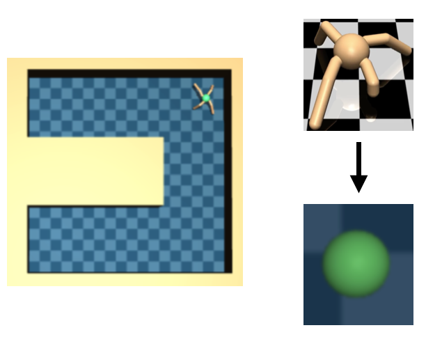
Figure 1: Left side: AntUMaze domain. Right side: Projecting high-dimensional ant into lower-dimensional point-mass.

The core OPE problem is to produce accurate policy value estimates under policy distribution shift. This problem is particularly difficult on tasks with high-dimensional state-spaces (Voloshin et al. 2021; Fu et al. 2021). For example, consider the AntUMaze problem illustrated on the left side of Figure 1. In this task, an ant-like robot with a high-dimensional state representation moves in a U-shaped maze and receives a reward only for reaching a specific $2$D coordinate goal location. The state-space of this task includes information such as $2$D location, ant limb angles, torso orientation etc., resulting in a $29$-dimensional state-space. The OPE task is to evaluate the performance of a particular policy’s ability to take the ant to the $2$D goal location using data that may be collected by different policies. Policy distribution shift is common in this type of high-dimensional task since the chances of different policies inducing similar limb angles, torso orientations, paths traversed etc. are incredibly slim. Notice, however, that while different policies may induce different body configurations, they may traverse similar $2$D paths since all (successful) policies must move the ant through roughly the same path to reach the goal. Moreover, the only critical information needed from the state-space to determine the ant’s per-step reward are its $2$D coordinates. Motivated by this observation, we propose to improve the accuracy of OPE algorithms on high-dimensional state-space tasks by projecting the high-dimensional state-space into a lower-dimensional space. This idea is illustrated on the right side of Figure 1 where the ant is reduced to a $2$D point-mass.

With this general motivation in mind, in this paper, we leverage concepts from the state abstraction literature (Li, Walsh, and Littman 2006) to improve the accuracy of marginalized importance sampling (MIS) OPE algorithms which estimate state-action density correction ratios to compute a policy value estimate (Liu et al. 2018a; Xie, Ma, and Wang 2019; Yin and Wang 2020). Due to the low chances of similarity between states of policies in high-dimensional state-spaces, current MIS algorithms can produce high variance state-action density ratios, resulting in high variance OPE estimates. However, if we are given a suitable state abstraction function, we can project the high-dimensional ground state-space into a lower-dimensional abstract state-space. The projection step increases the chances of similarity between these lower-dimensional states, resulting in low variance density ratios and OPE estimates. To the best of our knowledge, this work is the first to leverage concepts from state abstraction to improve OPE. We make the following contributions:

1. Theoretical analyses showing: (a) the variance of abstract state-action ratios is at most that of ground state-action ratios; and (b) that our abstract MIS OPE estimator is unbiased, strongly consistent, and can have lower variance than its ground equivalent.

2. An algorithm, based on a popular class of MIS algorithms, to estimate the abstract state-action ratios.

3. An empirical analysis of our estimator on a variety of high-dimensional state-space tasks.

2 Preliminaries

In this section, we discuss relevant background information.

2.1 Notation and Problem Setup

We consider an infinite-horizon Markov decision process (MDP), $\mathcal{M}=\langle\mathcal{S},\mathcal{A},\mathcal{R},P,\gamma,d_{0}\rangle$, where $\mathcal{S}$ is the state-space, $\mathcal{A}$ is the action-space, $\mathcal{R}:\mathcal{S}\times\mathcal{A}\to\Delta([0,\infty))$ is the reward function, $P:\mathcal{S}\times\mathcal{A}\to\Delta(\mathcal{S})$ is the transition dynamics function, $\gamma\in[0,1)$ is the discount factor, and $d_{0}\in\Delta(\mathcal{S})$ is the initial state distribution. The agent acting, according to policy $\pi$, in the MDP generates a trajectory: $s_{0},a_{0},r_{0},s_{1},a_{1},r_{1},...$, where $s_{0}\sim d_{0}$, $a_{t}\sim\pi(\cdot|s_{t})$, $r_{t}\sim\mathcal{R}(s_{t},a_{t})$, and $s_{t+1}\sim P(\cdot|s_{t},a_{t})$ for $t\geq 0$. We define $r(s,a):=\operatorname{\mathbb{E}}_{r\sim\mathcal{R}(s,a)}[r]$ and the agent’s discounted state-action occupancy measure under policy $\pi$ as $d_{\pi}$:

$$d_{\pi}(s,a):=\lim_{T\to\infty}\frac{\sum_{t=0}^{T-1}\gamma^{t}d_{\pi}(s_{t},a_{t})}{\sum_{t=0}^{T-1}\gamma^{t}}$$

where $d_{\pi}(s_{t},a_{t})$ is the probability the agent will be in state $s$ and take action $a$ at time-step $t$ under policy $\pi$.

In the infinite-horizon setting, we define the performance of policy $\pi$ to be its average reward, $\rho(\pi):=\operatorname{\mathbb{E}}_{(s,a)\sim d_{\pi},r\sim\mathcal{R}(s,a)}[r]$. Note that $\operatorname{\mathbb{E}}_{(s,a)\sim d_{\pi},r\sim\mathcal{R}(s,a)}[r]=(1-\gamma)\operatorname{\mathbb{E}}_{s_{0}\sim d_{0},a_{0}\sim\pi}[q^{\pi}(s_{0},a_{0})]$ where $q^{\pi}(s,a):=\operatorname{\mathbb{E}}[\sum_{k=0}^{\infty}\gamma^{t}r_{k+t}|s_{t}=s,a_{t}=a]$ is the action-value function which satisfies $q^{\pi}(s,a)=r(s,a)+\gamma\operatorname{\mathbb{E}}_{s^{\prime}\sim P(s,a),a^{\prime}\sim\pi(s^{\prime})}[q^{\pi}(s^{\prime},a^{\prime})]$.

2.2 Off-Policy Evaluation (OPE)

In behavior-agnostic off-policy evaluation (OPE), the goal is to estimate the performance of an evaluation policy $\pi_{e}$ given only a fixed offline data set of transition tuples, $\mathcal{D}:=\{(s_{i},a_{i},s_{i}^{\prime},r_{i})\}_{i=1}^{mT}$, where $(s_{i},a_{i})\sim d_{\mathcal{D}}$, $m$ is the batch size (number of trajectories), and $T$ is the fixed length of each trajectory, generated by unknown and possibly multiple behavior policies. The difficulty in OPE is to estimate $\rho(\pi_{e})$ under $d_{\pi_{e}}$ given samples only from $d_{\mathcal{D}}$.

We define the average-reward in dataset $\mathcal{D}$ to be $\bar{r}_{\mathcal{D}}:=\operatorname{\mathbb{E}}_{(s,a)\sim d_{\mathcal{D}},r\sim\mathcal{R}(s,a)}[r]$. As in prior OPE work, we assume that if $d_{\pi_{e}}(s,a)>0$ then $d_{\mathcal{D}}(s,a)>0$. Empirically, we measure the accuracy of an estimate $\hat{\rho}(\pi_{e})$ by generating $M$ datasets and then computing the relative mean-squared error (MSE): $\text{MSE}(\hat{\rho}(\pi_{e})):=\frac{1}{M}\sum_{i=1}^{M}\frac{\left(\rho(\pi_{e})-\hat{\rho_{i}}(\pi_{e})\right)^{2}}{\left(\rho(\pi_{e})-\bar{r}_{\mathcal{D}_{i}}\right)^{2}}$, where $\hat{\rho_{i}}(\pi_{e})$ is computed using dataset $\mathcal{D}_{i}$ and $\bar{r}_{\mathcal{D}_{i}}$ is the average reward in $\mathcal{D}_{i}$.

Marginalized Importance Sampling (MIS)

In this work, we focus on MIS methods, which evaluate $\pi_{e}$ by using the ratio between $d_{\pi_{e}}$ and $d_{\mathcal{D}}$. That is, MIS methods evaluate $\pi_{e}$ by estimating $\rho(\pi_{e}):=\operatorname{\mathbb{E}}_{(s,a)\sim d_{\mathcal{D}},r\sim\mathcal{R}(s,a)}[\zeta(s,a)r]$, where

$$\zeta(s,a):=\frac{d_{\pi_{e}}(s,a)}{d_{\mathcal{D}}(s,a)}$$

is the state-action density ratio for state-action pair $(s,a)$ and $d_{\pi}(s,a)=d_{\pi}(s)\pi(a|s)$. When the true $\zeta$ is known, the empirical estimate of $\rho(\pi_{e})$ is:

$$\hat{\rho}(\pi_{e}) :=\frac{1}{N}\sum_{i=1}^{N}\zeta(s_{i},a_{i})r(s_{i},a_{i})$$ (1)

where $N$ is the number of samples. In practice, however, $\zeta$ is unknown and must be estimated.

One set of $\zeta$-estimation algorithms, which have also shown potential for good OPE performance (Voloshin et al. 2021), is the DICE family (Yang et al. 2020). While there are many variations, the general DICE optimization problem is:

$$\begin{split}&\max_{\zeta:\mathcal{S}\times A\to\mathbb{R}}\min_{\nu:\mathcal{S}\times A\to\mathbb{R}}J(\zeta,\nu):=\\ &\operatorname{\mathbb{E}}_{(s,a,s^{\prime})\sim d_{\mathcal{D}},a^{\prime}\sim\pi_{e}}[\zeta(s,a)(\nu(s,a)-\gamma\nu(s^{\prime},a^{\prime}))]\\ &-(1-\gamma)\operatorname{\mathbb{E}}_{s_{0}\sim d_{0},a_{0}\sim\pi_{e}}[\nu(s_{0},a_{0})]\end{split}$$ (2)

where the solution to the optimization, $\zeta^{*}(s,a)$, are the true ratios. The estimator we present in Section 3 builds upon the DICE framework.

2.3 State Abstractions

We define a state abstraction function as a mapping $\phi:\mathcal{S}\to\mathcal{S}^{\phi}$, where $\mathcal{S}$ is called the ground state-space and $\mathcal{S}^{\phi}$ is called the abstract state-space. We consider state abstraction functions that partition the ground state-space into disjoint sets.

We can use $\phi$ to project the original MDP into a new abstract MDP with the same action-space $\mathcal{A}$ and reward and transition dynamics functions defined as:

$$\mathcal{R}^{\phi}(s^{\phi},a) =\sum_{s\in\phi^{-1}(s^{\phi})}w(s)\mathcal{R}(s,a)$$

$$P^{\phi}(s^{\prime\phi}|s^{\phi},a) =\sum_{s\in\phi^{-1}(s^{\phi}),s^{\prime}\in\phi^{-1}(s^{\prime\phi})}w(s)P(s^{\prime}|s,a)$$

where $w:\mathcal{S}\to[0,1]$ is a ground state weighting function where for each $s^{\phi}\in\mathcal{S}^{\phi}$, $\sum_{s\in\phi^{-1}(s^{\phi})}w(s)=1$ (Li, Walsh, and Littman 2006). Similarly a policy can be transformed into its abstract equivalent as:

$$\pi^{\phi}(a|s^{\phi}) =\sum_{s\in\phi^{-1}(s^{\phi})}w(s)\pi(a|s).$$

We define the following state-weighting function for an arbitrary policy $\pi$: $w_{\pi}(s)=\frac{d_{\pi}(s)}{\sum_{s^{\prime}\in\phi^{-1}(s^{\phi})}d_{\pi}(s^{\prime})}$ and only consider abstractions that satisfy:

Assumption 1 (Reward distribution equality).

$\forall s_{1},s_{2}\in\mathcal{S}$ such that $\phi(s_{1})=\phi(s_{2})$, $\forall a,\mathcal{R}(s_{1},a)=\mathcal{R}(s_{2},a)$.

Assumption 1 implies that, regardless of the choice of the state-weighting function, for given action $a$, $\forall s\in s^{\phi}$, $\mathcal{R}^{\phi}(s^{\phi},a)=\mathcal{R}(s,a)$ i.e. the reward distribution of an abstract state equals that of the ground states within that abstract state.

3 Abstract Marginalized Importance Sampling

Marginalized IS methods may suffer from high variance in high-dimensional state-spaces. To potentially reduce this high variance, we propose to first use $\phi$ to project $\mathcal{D}$ into the abstract state-space to obtain: $\mathcal{D}^{\phi}\coloneqq\{(s^{\phi},a,r^{\phi},s^{\prime}{{}^{\phi}})\}$ where $s^{\phi}=\phi(s)$ and $r^{\phi}(s^{\phi},a)=r(s,a)\forall s\in s^{\phi}$, and then use the following estimator on $\mathcal{D}^{\phi}$ to estimate $\rho(\pi_{e}^{\phi})$:

Definition 1 (Abstract estimator).

We define our estimator of $\rho(\pi^{\phi}_{e})$ as follows:

$$\hat{\rho}(\pi^{\phi}_{e}) :=\frac{1}{N}\sum_{i=1}^{N}\frac{d_{\pi^{\phi}_{e}}(s_{i}^{\phi},a_{i})}{d_{\mathcal{D}^{\phi}}(s_{i}^{\phi},a_{i})}r^{\phi}(s_{i}^{\phi},a_{i})$$ (3)

where $N$ is the number of samples, $d_{\pi^{\phi}}(s^{\phi},a)=d_{\pi^{\phi}}(s^{\phi})\pi^{\phi}(a|s^{\phi})$ with $d_{\pi^{\phi}}(s^{\phi})=\sum_{s\in\phi^{-1}(s^{\phi})}d_{\pi}(s)$ and $\pi^{\phi}$ constructed using $w_{\pi}$.

In the remainder of this section, we first give an example to build intuition for why the abstract ratios $\frac{d_{\pi^{\phi}_{e}}(s^{\phi},a)}{d_{\mathcal{D}^{\phi}}(s^{\phi},a)}$ can have lower variance than the ground ratios and then show theoretically that the OPE estimator given in Equation (3) is strongly consistent and can produce lower variance OPE estimates of $\rho(\pi_{e})$ than the ground equivalent (Equation (1)) when the true ratios are known. Finally, when the true abstract ratios are unknown, we identify sufficient conditions under which unbiased estimation of the ratios is possible and adapt an existing DICE algorithm to estimate them.

3.1 A Hard Example for Ground MIS Ratios

Figure 2: TwoPath MDP where ground density ratios for $(s_{1},a_{0})$ and $(s_{2},a_{0})$ are high variance. However, upon aggregation of equivalent states (grey dotted lines), the abstract density ratio of $(s^{\phi}_{1},a_{0})$ is low variance.

We present a hard example for ground MIS ratios in Figure 2 that provides intuition for why the abstract MIS ratios can have lower variance ratios than the ground ratios. Consider two symmetric policies, $\pi_{e}$ and $\pi_{\mathcal{D}}$, executed in the ground MDP (left side). In this example, the high variance of the true state-action density ratios $\frac{d_{\pi_{e}}(s_{1},a_{0})}{d_{\pi_{\mathcal{D}}}(s_{1},a_{0})}\approx 0$ and $\frac{d_{\pi_{e}}(s_{2},a_{0})}{d_{\pi_{\mathcal{D}}}(s_{2},a_{0})}\approx 100$ can lead to high variance estimates of $\rho(\pi_{e})$. Notice, however, that states $s_{1}$ and $s_{2}$ are essentially equivalent i.e. $r(s_{1},a)=r(s_{2},a)\forall a\in\mathcal{A}$ and can be aggregated together into a single state, $s^{\phi}_{1}$ (Assumption 1). We find that the state-action density ratio in this abstract MDP (right side) $\frac{d_{\pi^{\phi}_{e}}(s_{1}^{\phi},a_{0})}{d_{\pi^{\phi}_{\mathcal{D}}}(s_{1}^{\phi},a_{0})}=1$ is of low variance, which can lead to low variance estimates of $\rho(\pi_{e})$.

In general, we prove that the abstract ratios are guaranteed to have variance at most that of the ground ratios (proof in Appendix A.3):

Theorem 1.

$\text{Var}\left(\frac{d_{\pi^{\phi}_{e}}(s^{\phi},a)}{d_{\mathcal{D}^{\phi}}(s^{\phi},a)}\right)\leq\text{Var}\left(\frac{d_{\pi_{e}}(s,a)}{d_{\mathcal{D}}(s,a)}\right)$

where equality holds if either or both of the following are true: 1) $\phi$ is the identity function i.e. $\phi(s)=s,\forall s\in\mathcal{S}$ and 2) if $\forall s_{1},s_{2}\in\mathcal{S}$ such that $\phi(s_{1})=\phi(s_{2})=s^{\phi}$ and for a given action $a$, $\frac{d_{\pi_{e}}(s_{1},a)}{d_{\mathcal{D}}(s_{1},a)}=\frac{d_{\pi_{e}}(s_{2},a)}{d_{\mathcal{D}}(s_{2},a)},\forall s^{\phi}\in\mathcal{S}^{\phi},a\in\mathcal{A}$. Thus, Theorem 1 implies that projecting $\mathcal{S}\to\mathcal{S}^{\phi}$ can lower the variance of density ratios.

3.2 MIS OPE with True Abstract Ratios

We now present the statistical properties of our estimator assuming it has access to the true abstract state-action ratios. Due to space constraints, we defer proofs to Appendix A.3.

We prove our abstract estimator is unbiased (Theorem 4 in Appendix A.3) and strongly consistent (Theorem 2 and Corollary 1):

Theorem 2.

Our estimator, $\hat{\rho}(\pi^{\phi}_{e})$, given in Equation 3 is an asymptotically consistent estimator of $\rho(\pi_{e})$ in terms of MSE: $\lim_{N\to\infty}\operatorname{\mathbb{E}}[(\hat{\rho}(\pi^{\phi}_{e})-\rho(\pi_{e}))^{2}]=0$.

We also compare the variances between our abstract estimator and the ground equivalent. If we assume that $\mathcal{D}$ is i.i.d as done in previous work (Sutton et al. 2008; Uehara, Huang, and Jiang 2019; Nachum et al. 2019; Zhang et al. 2020), then $\text{Var}(\hat{\rho}(\pi^{\phi}_{e}))\leq\text{Var}(\hat{\rho}(\pi_{e}))$, where equality holds only under the same conditions as described below Theorem 1. In general, however, variance reduction depends on the covariances between the weighted per-step rewards (Liu, Bacon, and Brunskill 2019):

Theorem 3.

If Assumption 1 and if for any fixed $1\leq t<k\leq T$, $\text{Cov}\left(\frac{d_{\pi^{\phi}_{e}}(s_{t}^{\phi},a_{t})}{d_{\mathcal{D}^{\phi}}(s_{t}^{\phi},a_{t})}r^{\phi}(s_{t}^{\phi},a_{t}),\frac{d_{\pi^{\phi}_{e}}(s_{k}^{\phi},a_{k})}{d_{\mathcal{D}^{\phi}}(s_{k}^{\phi},a_{k})}r^{\phi}(s_{k}^{\phi},a_{k})\right)\leq\text{Cov}\left(\frac{d_{\pi_{e}}(s_{t},a_{t})}{d_{\mathcal{D}}(s_{t},a_{t})}r(s_{t},a_{t}),\frac{d_{\pi_{e}}(s_{k},a_{k})}{d_{\mathcal{D}}(s_{k},a_{k})}r(s_{k},a_{k})\right)$ hold then $\text{Var}(\hat{\rho}(\pi^{\phi}_{e}))\leq\text{Var}(\hat{\rho}(\pi_{e}))$.

3.3 Estimating the Abstract Ratios

Thus far, we have assumed access to the true abstract ratios. However, in practice, these ratios are unknown and must be estimated from $\mathcal{D}^{\phi}$. In this section, we highlight the challenges in estimating the abstract ratios and identify sufficient conditions on $\phi$ that allow for accurate estimation. Once $\phi$ satisfies these conditions, any off-the-shelf state-action density estimation method can be used to estimate the abstract ratios. In this work, we focus on showing that DICE estimates the true abstract ratios. We note that the following new conditions on $\phi$ are only needed for unbiased estimation of the abstract ratios; accurate OPE on the abstracted MDP can still be realized under only Assumption 1.

We first observe that evaluating $\pi_{e}$ using $\mathcal{D}$ is equivalent to evaluating $\pi^{\phi}_{e}$ using $\mathcal{D}^{\phi}$ if $\mathcal{D}^{\phi}$ is generated from an abstract MDP with transition dynamics constructed according to $w_{\pi_{e}}$. This equivalence is given by the following proposition:

Proposition 1.

If Assumption 1 holds, the average reward of ground policy $\pi$ executed in ground MDP $\mathcal{M}$, $\rho(\pi)$, is equal to the average reward of abstract policy $\pi^{\phi}$ executed in abstract MDP $\mathcal{M}^{\phi}$ constructed with $w_{\pi}$, $\rho(\pi^{\phi})$. That is, $\rho(\pi)=\rho(\pi^{\phi})$.

Proposition 1 suggests that we can estimate $\rho(\pi_{e})$ by applying any OPE algorithm to evaluate $\pi_{e}^{\phi}$ using $\mathcal{D}^{\phi}$ if the abstract transition dynamics of $\mathcal{D}^{\phi}$ are distributed according to $P_{w_{\pi_{e}}}^{\phi}$. Unfortunately, since $w_{\pi_{e}}$ is unknown, two challenges arise. Fortunately, there are special cases where unbiased estimation of the abstract ratios is still possible using only existing MIS algorithms.

Challenge 1: Transition dynamics distribution shift. The off-policy data $\mathcal{D}^{\phi}:=\{(s^{\phi},a,r^{\phi},s^{\prime\phi})\}$ is distributed in the following way: $(s^{\phi},a)\sim d_{\mathcal{D}^{\phi}},r^{\phi}\sim\mathcal{R}^{\phi},s^{\prime\phi}\sim P^{\phi}_{w_{\mathcal{D}}}(s^{\phi},a)$ where $P_{w_{\mathcal{D}}}^{\phi}$ are the transition dynamics of the abstract MDP constructed with $w_{\mathcal{D}}$ as the state-weighting function. Thus, in addition to the original policy distribution shift problem, we also encounter a transition dynamics distribution shift problem due to the projection where we want to evaluate $\pi^{\phi}_{e}$ in an MDP with $P_{w_{\pi_{e}}}^{\phi}$, but we only have samples of data generated in an MDP with $P_{w_{\mathcal{D}}}^{\phi}$. Moreover, since $w_{\pi_{e}}$ is unknown, we cannot compute $P_{w_{\pi_{e}}}^{\phi}$ and correct the distribution shift, say through importance sampling (Precup, Sutton, and Singh 2000), as we would correct for policy distribution shift. However, one condition on $\phi$ that will avoid the transition distribution shift is:

Assumption 2 (Transition dynamics similarity).

$\forall s_{1},s_{2}\in\mathcal{S}$ such that $\phi(s_{1})=\phi(s_{2})$, $\forall a\in\mathcal{A},x\in\mathcal{S}^{\phi}$, we have $\sum_{s^{\prime}\in\phi^{-1}(x)}P(s^{\prime}|s_{1},a)=\sum_{s^{\prime}\in\phi^{-1}(x)}P(s^{\prime}|s_{2},a)$.

Together with Assumption 1, $\phi$ is now the so-called bisimulation abstraction (Ferns, Panangaden, and Precup 2011; Castro 2020). This property of $\phi$ eliminates the transition dynamics distribution shift since now $P_{w_{\pi_{e}}}^{\phi}(s^{\prime\phi}|s^{\phi},a)=P_{w_{\mathcal{D}}}^{\phi}(s^{\prime\phi}|s^{\phi},a)=P^{\phi}(s^{\prime\phi}|s^{\phi},a)=\sum_{s^{\prime}\in s^{\prime\phi}}P(s^{\prime}|s,a)\forall s\in s^{\phi},\forall a\in\mathcal{A}$ (applying Assumption 2 and definition of $P^{\phi}$ from Section 2.3). Thus, we have $\mathcal{D}^{\phi}$ distributed with $P_{w_{\pi_{e}}}^{\phi}=P^{\phi}$, which then allows us to apply any MIS algorithm to compute the abstract state-action ratios using $\mathcal{D}^{\phi}$.

Challenge 2: Inaccessible $\pi^{\phi}_{e}$. To the best of our knowledge, all existing MIS algorithms require access to the evaluation policy to estimate the density ratios. However, in the abstract MDP, $\pi^{\phi}_{e}$ is inaccessible since $w_{\pi_{e}}$ is unknown. To overcome this issue, we identify the following condition on $\phi$:

Assumption 3 ($\pi_{e}$ action-distribution equality).

$\forall s_{1},s_{2}\in\mathcal{S}$ such that $\phi(s_{1})=\phi(s_{2})$, $\pi_{e}(s_{1})=\pi_{e}(s_{2})$

Assumption 3 then gives us $\pi^{\phi}_{e}(s^{\phi})=\pi_{e}(s),\forall s\in s^{\phi}$ (applying Assumption 3 and definition of $\pi^{\phi}$ from Section 2.3), which allows us to simulate sampling from $\pi^{\phi}_{e}(\cdot|\phi(s))$ by just sampling from $\pi_{e}(\cdot|s)$.

Given a $\phi$ with these properties, we can compute the abstract ratios needed to estimate $\rho(\pi_{e})$ by applying a suitable MIS algorithm to $\mathcal{D}^{\phi}$. We use BestDICE (Yang et al. 2020), and call our algorithm AbstractBestDICE, which solves the following optimization problem:

$$\begin{split}&\min_{\nu,\lambda}\max_{\zeta}J(\nu,\zeta,\lambda):=-\operatorname{\mathbb{E}}_{\mathcal{D}^{\phi}}\left[\frac{1}{2}\zeta(s^{\phi},a)^{2}\right]\\ &+\operatorname{\mathbb{E}}_{\mathcal{D}^{\phi}}\left[\zeta(s^{\phi},a)\left(\gamma\operatorname{\mathbb{E}}_{a^{\prime}\sim\pi^{\phi}_{e}}[\nu(s^{\prime\phi},a^{\prime})]-\nu(s^{\phi},a)-\lambda\right)\right]\\ &+(1-\gamma)\operatorname{\mathbb{E}}_{s^{\phi}_{0}\sim d_{0^{\phi}},a_{0}\sim\pi^{\phi}_{e}}[\nu(s^{\phi}_{0},a_{0})]+\lambda\end{split}$$ (4)

where, $\nu:\mathcal{S}^{\phi}\times\mathcal{A}\to\mathbb{R}$, $\lambda\in\mathbb{R}$, and $\zeta:\mathcal{S}^{\phi}\times\mathcal{A}\to\mathbb{R}_{\geq 0}$. The solution to the optimization, $\zeta^{*}(s^{\phi},a)=d_{\pi^{\phi}_{e}}(s^{\phi},a)/d_{\mathcal{D}^{\phi}}(s^{\phi},a)$ is the true abstract ratios. Since the derivation of AbstractBestDICE follows the same steps as BestDICE, we defer it to Appendix A.4.

We note that it may be difficult to validate Assumptions 2 and 3 in practice, which may result in loss of the consistency guarantee of Theorem 2. Nevertheless, in Section 4 we show that AbstractBestDICE leads to accurate OPE in high-dimensional state-spaces even when assumptions may not hold.

4 Empirical Study

We will now show how projecting $\mathcal{S}\to\mathcal{S}^{\phi}$ can produce more accurate OPE estimates in practice. We answer the following questions:

1. Do the true abstract ratios produce lower variance OPE estimates than the true ground ratios?

2. Does AbstractBestDICE: (a) compute the true ratios when Assumptions 1, 2, and 3 are satisfied and (b) produce data-efficient and stable estimates of $\rho(\pi_{e})$ even when Assumptions 2 and 3 fail to hold?

4.1 Empirical Setup

In this section, we describe the algorithms and domains of our empirical study. Due to space constraints, we defer specific details to the appendix (A.5 and A.6).

Algorithms

We compare AbstractBestDICE to ground BestDICE (Yang et al. 2020). As also reported by Yang et al. (2020); Fu et al. (2021), we found in preliminary experiments (see Appendix A.6) that BestDICE performed much better than other MIS methods such as DualDICE (Nachum et al. 2019), Minimax-Weight Learning (Uehara, Huang, and Jiang 2019), etc.

Domains

We focus on high-dimensional state-space tasks, which have been known to be particularly challenging for DICE methods (Fu et al. 2021). For each environment below we specify a fixed $\phi$.

• TwoPath MDP. This MDP is pictured in Figure 2. In this domain, Assumptions 1, 2, and 3 are satisfied. We also run the same experiments for when these assumptions are violated (see Appendix A.5).

• Reacher (Brockman et al. 2016). A robotic arm tries to move to a goal location. Here, $s\in\mathbb{R}^{11}$ and $a\in\mathbb{R}^{2}$. Since the reward function is the Euclidean distance between the arm and goal, $\phi$ extracts only the arm-to-goal vector, and angular velocities from the ground state, resulting in $s^{\phi}\in\mathbb{R}^{4}$.

• Walker2D (Brockman et al. 2016). A bi-pedal robot tries to move as fast as possible. Here, $s\in\mathbb{R}^{18}$ and $a\in\mathbb{R}^{6}$. We use the Euclidean distance from the start location as the reward function and use a $\phi$ that extracts $x$ and $z$ coordinates and top angle of the walker’s body, resulting in $s^{\phi}\in\mathbb{R}^{3}$.

• Pusher (Brockman et al. 2016). A robotic arm tries to push an object to a goal location. Here, $s\in\mathbb{R}^{23}$ and $a\in\mathbb{R}^{7}$. Since the reward function is the Euclidean distance between object and arm and object and goal, $\phi$ extracts only object-to-arm and object-to-goal vectors, resulting in $s^{\phi}\in\mathbb{R}^{6}$.

• AntUMaze (Fu et al. 2020). This sparse-reward task requires an ant to move from one end of the U-shaped maze to the other end. Here, $s\in\mathbb{R}^{29}$ and $a\in\mathbb{R}^{8}$. We use the “play” version where the goal location is fixed. Since the reward function is $+1$ only if the $2$D location of the ant is at a certain Euclidean distance from the $2$D goal location, $\phi$ extracts only the $2$D coordinates of the ant, resulting in $s^{\phi}\in\mathbb{R}^{2}$.

For Reacher, Walker2D, Pusher, and AntUMaze, $\phi$ satisfies only Assumption 1.

4.2 Empirical Results

In this section, we describe our main empirical results; additional experiments can be found in appendix A.6.

True Ratios for OPE

We conduct an experiment on the TwoPath MDP to estimate $\rho(\pi_{e})$ where we apply the ground estimator given in Equation (1) and our abstract estimator given in Equation (3), assuming both have access to their respective true ratios. The results of this experiment are illustrated in Figure 3(a). We can observe that the abstract estimator with the true abstract ratios produces substantially more data-efficient and lower variance OPE estimates for different batch sizes compared to the ground equivalent.

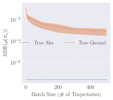
(a) MSE vs. Batch size (# of trajectories). The vertical axis axis is log-scaled. Errors are computed over $15$ trials with $95\%$ confidence intervals. Lower is better. Since $\rho(\pi_{e})=\rho(\pi_{\mathcal{D}})$ in this domain, we use regular MSE instead of relative.

(b) Estimated $\hat{d}_{\pi^{\phi}_{e}}$ (vertical axis) vs. true $d_{\pi^{\phi}_{e}}$ (horizontal axis). Values are averaged over $15$ trials. We expect the dots to be as close to the black line as possible. Each dot is for each $(s^{\phi},a)$. Dots are only at extreme ends due to choice of $\pi_{e}$, $\pi_{\mathcal{D}}$, and ToyMDP design. Only $4$ out of $6$ dots are visible due to overlap between the dots for $(s_{1}^{\phi},a_{1})$ and $(s_{2}^{\phi},a_{1})$, and $(s_{1}^{\phi},a_{0})$ and $(s_{2}^{\phi},a_{0})$.

Figure 3: True ratio experiments.

True Ratio Estimation

To verify if AbstractBestDICE accurately estimates the true ratios we conduct the following experiment on the TwoPath MDP. We give AbstractBestDICE data of batch size $300$ to estimate the abstract ratios $\hat{\zeta}^{\phi}$ and then use $\hat{\zeta}^{\phi}$ to estimate the abstract state-action densities of $\pi^{\phi}_{e}$, $\hat{d}_{\pi^{\phi}_{e}}(s^{\phi},a)=\hat{\zeta}^{\phi}(s^{\phi},a)d_{\pi^{\phi}_{\mathcal{D}}}(s^{\phi},a)$, where we have access to the true $d_{\pi^{\phi}_{\mathcal{D}}}(s^{\phi},a)$. We then compare $\hat{d}_{\pi^{\phi}_{e}}$ to the true $d_{\pi^{\phi}_{e}}$, which we compute using a batch size of $300$ trajectories collected from $\pi^{\phi}_{e}$ roll-outs, using a correlation plot shown in Figure 3(b). From the figure we can see AbstractBestDICE accurately estimates the abstract state-action density ratios. When assumptions are violated, however, ratio estimation accuracy can reduce (see Appendix A.5).

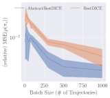
(a) Reacher

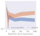
(b) Walker2D

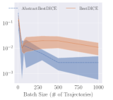
(c) Pusher

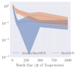
(d) AntUMaze

Figure 4: Relative MSE vs. Batch Size (# of trajectories). Vertical axis is log-scaled. Errors are computed over $15$ trials with $95\%$ confidence intervals. Lower is better.

Data-Efficiency

Figure 4 shows the results of our (relative) MSE vs. batch size experiment for the function approximation case. For a given batch size, we train each algorithm for $100$k epochs with different hyperparameters sets, record the (relative) MSE on the last epoch by each hyperparameter set, and plot the lowest MSE achieved by these hyperparameter sets. We find that AbstractBestDICE is able to achieve lower MSE than BestDICE for a given batch size. We note that while hyperparameter tuning is difficult in OPE, in this experiment, we aim to evaluate the performance of each algorithm assuming both had favorable hyperparameters.

Hyperparameter Robustness

Finally, we study the robustness of these algorithms to hyperparameters tuning. In practical OPE, hyperparameter tuning with respect to MSE is impractical since the true $\rho(\pi_{e})$ is unknown (Fu et al. 2021; Paine et al. 2020). Thus, we want OPE algorithms to be as robust as possible to hyperparameter tuning. The main hyperparameters for DICE are the learning rates of $\zeta$ and $\nu$, $\alpha_{\zeta}$ and $\alpha_{\nu}$. For these experiments, we focus on very small batch sizes, where we would expect high sensitivity. The results of this study are in Figure 5. We find that our algorithm has a less volatile MSE than BestDICE (also see appendix A.6 for more similar results). In a related experiment, we also find AbstractBestDICE can be more stable than BestDICE during training (see appendix A.6).

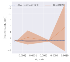
Figure 5: Robustness of BestDICE and AbstractBestDICE to hyperparameters on the AntUMaze domain for batch size (# of trajectories) of $5$. Errors are computed over $15$ trials with $95\%$ confidence intervals. Lower is better.

5 Related Work

MIS and Off-Policy Evaluation. There have been broadly three families of MIS algorithms in the OPE literature to estimate state-action density ratios. One is the DICE family, which includes: minimax-weight learning (Uehara, Huang, and Jiang 2019), DualDice (Nachum et al. 2019), GenDICE (Zhang et al. 2020), GradientDICE  (Zhang, Liu, and Whiteson 2020), and BestDICE (Yang et al. 2020). In our work, we adapt BestDICE to estimate the abstract ratios. The second family of MIS algorithms is the COP-TD algorithm (Hallak and Mannor 2017; Gelada and Bellemare 2019), which learns the state density ratios with an online TD-styled update. The third family is the variational power method (Wen et al. 2020) algorithm which generalizes the power iteration method to estimate density ratios. While our focus has been on MIS algorithms, there are many other OPE algorithms such as model-based methods (Zhang et al. 2021b; Hanna, Stone, and Niekum 2017; Liu et al. 2018b), fitted-Q evaluation (Le, Voloshin, and Yue 2019), doubly-robust methods (Jiang and Li 2015; Thomas and Brunskill 2016), and IS (Precup, Sutton, and Singh 2000; Thomas 2015; Hanna, Niekum, and Stone 2019; Thomas, Theocharous, and Ghavamzadeh 2015).

State Abstraction and Representation Learning. The literature on state abstraction is extensive (Singh, Jaakkola, and Jordan 1994; Dietterich 1999; Ferns, Panangaden, and Precup 2011; Li, Walsh, and Littman 2006; Abel 2020). However, much of this work has been exclusively focused on building a theory of abstraction and on learning optimal policies. A related topic to state abstraction is representation learning. Recently, there has been much work showing the importance of good representations for offline RL (Wang et al. 2021; Yin et al. 2022; Geng et al. 2022; Zhan et al. 2022; Chen and Jiang 2022). To the best of our knowledge, no work has leveraged state abstraction techniques to improve the accuracy of OPE algorithms.

6 Summary and Future Work

In this work, we showed that we can improve the accuracy of OPE estimates by projecting the original ground state-space into a lower-dimensional abstract state-space using state abstraction and performing OPE in the resulting abstract Markov decision process. Our theoretical results proved that: 1) abstract state-action ratios have variance at most that of the ground ratios; and 2) the abstract MIS OPE estimator is unbiased, strongly consistent, and can have lower variance than the ground equivalent. We then highlighted the challenges that arise when estimating the abstract ratios from data, identified sufficient conditions to overcome these issues, and adapted BestDICE into AbstractBestDICE to estimate the abstract ratios. In our empirical results, we obtained more accurate OPE estimates with added hyperparameter robustness on difficult, high-dimensional state-space tasks.

There are several directions for future work. First, Assumptions 2 and 3 are strict. Further investigation is needed to see if these assumptions can be relaxed. Second, we assumed the abstraction function was given. It would be interesting to leverage existing ideas (Gelada et al. 2019; Zhang et al. 2021a) to learn $\phi$. Finally, we want to emphasize that this work instantiates the general abstraction + OPE direction. While this work focused exclusively on MIS algorithms, a promising direction will be to apply abstraction techniques to model-based, trajectory IS, and value-function based OPE.

Appendix A Appendix

A.1 Preliminaries

This section provides the supporting lemmas and definitions that we leverage to prove our lemmas and theorems.

Definition 2 (Almost Sure Convergence).

A sequence of random variables, $(X_{n})_{n=1}^{\infty}$, almost surely converges to the random variable, $X$ if

$$\operatorname{\mathbb{P}}\left(\lim_{n\to\infty}X_{n}=X\right)=1$$

We write $X_{n}\overset{a.s.}{\to}X$ to denote that the sequence $(X_{n})_{n=1}^{\infty}$ converges almost surely to $X$.

Definition 3 ((Strongly) Consistent Estimator).

Let $\theta$ be a real number and $(\hat{\theta}_{n})_{n=1}^{\infty}$ be an infinite sequence of random variables. We call $\hat{\theta}_{n}$ a (strongly) consistent estimator of $\theta$ if and only if $\hat{\theta}_{n}\overset{a.s.}{\to}\theta$.

Lemma 1.

If $(X_{i})_{i=1}^{\infty}$ is a sequence of uniformly bounded real-valued random variables, then $X_{n}\overset{a.s.}{\to}X$ if and only if $\lim_{N\to\infty}\operatorname{\mathbb{E}}[(X_{n}-X)^{2}]=0$.

Proof    See Lemma 3 in Thomas and Brunskill (2016). ∎

A.2 Assumptions and Definitions

In the main paper, we provided the major assumptions required for our theoretical and empirical work relevant to abstraction and OPE. Here we provide supporting assumptions typically used in the OPE literature used for the theoretical analysis.

Assumption 4 (Coverage).

For all $(s,a)\in\mathcal{S}\times\mathcal{A}$, if $\pi_{e}(a|s)>0$ then $\pi_{b}(a|s)>0$.

Assumption 5 (Non-negative reward).

We assume that the reward function is bounded between $[0,\infty)$.

Definition 4 (Ground state normalized weightings).

For a given policy $\pi$, each ground state $s\in s^{\phi}$, has a state aggregation weight, $w_{\pi}(s)=\frac{d_{\pi}(s)}{\sum_{s^{\prime}\in\phi^{-1}(s^{\phi})}d_{\pi}(s^{\prime})}$, where $d_{\pi}(s)$ is the discounted state-occupancy measure of $\pi$.

A.3 Proofs

In the proofs below, we denote the collection of behavior policies that generated $\mathcal{D}$ with $\pi_{\mathcal{D}}$. That is, $\pi_{\mathcal{D}}$ is the conditional probability of an action occurring in a given state in the data. Similarly, we also have $\pi^{\phi}_{\mathcal{D}}$. These minor changes give us $d_{\mathcal{D}}=d_{\pi_{\mathcal{D}}}$ and $d_{\mathcal{D}^{\phi}}=d_{\pi^{\phi}_{\mathcal{D}}}$.

Lemma 2.

For an arbitrary function, $f$, $\operatorname{\mathbb{E}}_{s^{\phi}\sim d_{\pi^{\phi}},a\sim\pi^{\phi}}\left[f(s^{\phi},a)\right]=\operatorname{\mathbb{E}}_{s\sim d_{\pi},a\sim\pi}\left[f(\phi(s),a)\right]$.

Proof

$$\operatorname{\mathbb{E}}_{s^{\phi}\sim d_{\pi^{\phi}},a\sim\pi^{\phi}}\left[f(s^{\phi},a)\right] =\sum_{s^{\phi},a}d_{\pi^{\phi}}(s^{\phi})\pi^{\phi}(a|s^{\phi})f(s^{\phi},a)$$

$$\stackrel{{\scriptstyle\textnormal{(a)}}}{{\mathstrut{=}}}\sum_{s^{\phi},a}d_{\pi^{\phi}}(s^{\phi})\sum_{s\in\phi^{-1}(s^{\phi})}\frac{\pi(a|s)d_{\pi}(s)}{d_{\pi^{\phi}}(s^{\phi})}f(s^{\phi},a)$$

$$=\sum_{s^{\phi},a}\sum_{s\in\phi^{-1}(s^{\phi})}\pi(a|s)d_{\pi}(s)f(s^{\phi},a)$$

$$=\sum_{s,a}\pi(a|s)d_{\pi}(s)f(\phi(s),a)$$

$$\operatorname{\mathbb{E}}_{s^{\phi}\sim d_{\pi}^{\phi},a\sim\pi^{\phi}}\left[f(s^{\phi},a)\right] =\operatorname{\mathbb{E}}_{s\sim d_{\pi},a\sim\pi}\left[f(\phi(s),a)\right]$$

where (A.3) is due to Definition 4 and we can replace $s^{\phi}$ with $\phi(s)$ when we know $s\in s^{\phi}$. ∎

See 1 Proof

Before comparing the variances, we note that due to Assumption 4 and Lemma 2:

$$\operatorname{\mathbb{E}}_{s\sim d_{\pi_{\mathcal{D}}},a\sim\pi_{\mathcal{D}}}\left[\frac{d_{\pi_{e}}(s)\pi_{e}(a|s)}{d_{\pi_{\mathcal{D}}}(s)\pi_{\mathcal{D}}(a|s)}\right]=\operatorname{\mathbb{E}}_{s\sim d_{\pi^{\phi}_{\mathcal{D}}},a\sim\pi^{\phi}_{\mathcal{D}}}\left[\frac{d_{\pi^{\phi}_{e}}(s^{\phi})\pi^{\phi}_{e}(a|s^{\phi})}{d_{\pi^{\phi}_{\mathcal{D}}}(s^{\phi})\pi^{\phi}_{\mathcal{D}}(a|s^{\phi})}\right]=1$$

Denote, $V^{g}:=\text{Var}\left(\frac{d_{\pi_{e}}(s)\pi_{e}(a|s)}{d_{\pi_{\mathcal{D}}}(s)\pi_{\mathcal{D}}(a|s)}\right)$ and $V^{\phi}:=\text{Var}\left(\frac{d_{\pi^{\phi}_{e}}(s^{\phi})\pi^{\phi}_{e}(a|s^{\phi})}{d_{\pi^{\phi}_{\mathcal{D}}}(s^{\phi})\pi^{\phi}_{\mathcal{D}}(a|s^{\phi})}\right)$. Now consider the difference between the two variances.

$$D =V^{g}-V^{\phi}$$

$$=\text{Var}\left(\frac{d_{\pi_{e}}(s)\pi_{e}(a|s)}{d_{\pi_{\mathcal{D}}}(s)\pi_{\mathcal{D}}(a|s)}\right)-\text{Var}\left(\frac{d_{\pi^{\phi}_{e}}(s^{\phi})\pi^{\phi}_{e}(a|s^{\phi})}{d_{\pi^{\phi}_{\mathcal{D}}}(s^{\phi})\pi^{\phi}_{\mathcal{D}}(a|s^{\phi})}\right)$$

$$=\operatorname{\mathbb{E}}_{s\sim d_{\pi_{\mathcal{D}}},a\sim\pi_{\mathcal{D}}}\left[\left(\frac{d_{\pi_{e}}(s)\pi_{e}(a|s)}{d_{\pi_{\mathcal{D}}}(s)\pi_{\mathcal{D}}(a|s)}\right)^{2}\right]-\operatorname{\mathbb{E}}_{s^{\phi}\sim d_{\pi^{\phi}_{\mathcal{D}}},a\sim\pi_{\mathcal{D}}^{\phi}}\left[\left(\frac{d_{\pi^{\phi}_{e}}(s^{\phi})\pi^{\phi}_{e}(a|s^{\phi})}{d_{\pi^{\phi}_{\mathcal{D}}}(s^{\phi})\pi^{\phi}_{\mathcal{D}}(a|s^{\phi})}\right)^{2}\right]$$

$$=\sum_{s,a}d_{\pi_{\mathcal{D}}}(s)\pi_{\mathcal{D}}(a|s)\left(\frac{d_{\pi_{e}}(s)\pi_{e}(a|s)}{d_{\pi_{\mathcal{D}}}(s)\pi_{\mathcal{D}}(a|s)}\right)^{2}-\sum_{s^{\phi},a}d_{\pi^{\phi}_{\mathcal{D}}}(s^{\phi})\pi^{\phi}_{\mathcal{D}}(a|s^{\phi})\left(\frac{d_{\pi^{\phi}_{e}}(s^{\phi})\pi^{\phi}_{e}(a|s^{\phi})}{d_{\pi^{\phi}_{\mathcal{D}}}(s^{\phi})\pi^{\phi}_{\mathcal{D}}(a|s^{\phi})}\right)^{2}$$

$$=\sum_{s^{\phi},a}\left(\sum_{s\in s^{\phi}}d_{\pi_{\mathcal{D}}}(s)\pi_{\mathcal{D}}(a|s)\left(\frac{d_{\pi_{e}}(s)\pi_{e}(a|s)}{d_{\pi_{\mathcal{D}}}(s)\pi_{\mathcal{D}}(a|s)}\right)^{2}-d_{\pi^{\phi}_{\mathcal{D}}}(s^{\phi})\pi^{\phi}_{\mathcal{D}}(a|s^{\phi})\left(\frac{d_{\pi^{\phi}_{e}}(s^{\phi})\pi^{\phi}_{e}(a|s^{\phi})}{d_{\pi^{\phi}_{\mathcal{D}}}(s^{\phi})\pi^{\phi}_{\mathcal{D}}(a|s^{\phi})}\right)^{2}\right)$$

We can analyze this difference by looking at one abstract state and one action and all the states that belong to it. That is, for a fixed abstract state, $s^{\phi}$, and fixed action, $a$, we have:

$$D^{\prime} =\sum_{s\in s^{\phi}}d_{\pi_{\mathcal{D}}}(s)\pi_{\mathcal{D}}(a|s)\left(\frac{d_{\pi_{e}}(s)\pi_{e}(a|s)}{d_{\pi_{\mathcal{D}}}(s)\pi_{\mathcal{D}}(a|s)}\right)^{2}-\left(d_{\pi^{\phi}_{\mathcal{D}}}(s^{\phi})\pi^{\phi}_{\mathcal{D}}(a|s^{\phi})\left(\frac{d_{\pi^{\phi}_{e}}(s^{\phi})\pi^{\phi}_{e}(a|s^{\phi})}{d_{\pi^{\phi}_{\mathcal{D}}}(s^{\phi})\pi^{\phi}_{\mathcal{D}}(a|s^{\phi})}\right)^{2}\right)$$

$$=\left(\sum_{s\in s^{\phi}}\frac{(d_{\pi_{e}}(s)\pi_{e}(a|s))^{2}}{d_{\pi_{\mathcal{D}}}(s)\pi_{\mathcal{D}}(a|s)}\right)-\left(\frac{(d_{\pi^{\phi}_{e}}(s^{\phi})\pi^{\phi}_{e}(a|s^{\phi}))^{2}}{d_{\pi^{\phi}_{\mathcal{D}}}(s^{\phi})\pi^{\phi}_{\mathcal{D}}(a|s^{\phi})}\right)$$

$$\stackrel{{\scriptstyle\textnormal{(b)}}}{{\mathstrut{=}}}\left(\left(\sum_{s\in s^{\phi}}\frac{(d_{\pi_{e}}(s)\pi_{e}(a|s))^{2}}{d_{\pi_{\mathcal{D}}}(s)\pi_{\mathcal{D}}(a|s)}\right)-\left(\frac{(d_{\pi^{\phi}_{e}}(s^{\phi})\pi^{\phi}_{e}(a|s^{\phi})^{2}}{d_{\pi^{\phi}_{\mathcal{D}}}(s^{\phi})\pi^{\phi}_{\mathcal{D}}(a|s^{\phi})}\right)\right)$$

where (A.3) is due to Definition 4.

If we can show that $D^{\prime}\geq 0$ for all possible sizes of $|s^{\phi}|$, we will the have the original difference, $D$, is a sum of only non-negative terms, thus proving Theorem 1. We will prove $D^{\prime}\geq 0$ by inductive proof on the size of $|s^{\phi}|$ from $1$ to some $n\leq|\mathcal{S}|$.

Let our statement to prove, $P(n)$ be that $D^{\prime}\geq 0$ where $n=|s^{\phi}|$. This is trivially true for $P(1)$ where the ground state equals the abstract state. Now consider the inductive hypothesis, $P(n)$ is true for $n\geq 1$. Now with the inductive step, we must show that $P(n+1)$ is true given $P(n)$ is true. Starting with the inductive hypothesis:

$$D^{\prime\prime} =\underbrace{\left(\sum_{s\in s^{\phi}}\frac{(d_{\pi_{e}}(s)\pi_{e}(a|s))^{2}}{d_{\pi_{\mathcal{D}}}(s)\pi_{\mathcal{D}}(a|s)}\right)}_{S}-\left(\frac{(\overbrace{(d_{\pi^{\phi}_{e}}(s^{\phi})\pi^{\phi}_{e}(a|s^{\phi})}^{C})^{2}}{\underbrace{d_{\pi^{\phi}_{\mathcal{D}}}(s^{\phi})\pi^{\phi}_{\mathcal{D}}(a|s^{\phi})}_{C^{\prime}}}\right)\geq 0$$

We define $S:=\left(\sum_{s\in s^{\phi}}\frac{(d_{\pi_{e}}(s)\pi_{e}(a|s))^{2}}{d_{\pi_{\mathcal{D}}}(s)\pi_{\mathcal{D}}(a|s)}\right)$, $C:=(d_{\pi^{\phi}_{e}}(s^{\phi})\pi^{\phi}_{e}(a|s^{\phi})$, and $C^{\prime}:=d_{\pi^{\phi}_{\mathcal{D}}}(s^{\phi})\pi^{\phi}_{\mathcal{D}}(a|s^{\phi})$. After making the substitutions, we have:

$$C^{2}\leq SC^{\prime}$$ (5)

We have the above result holding true for when the $|s^{\phi}|=n$. Now consider the inductive step in relation to the inductive hypothesis where a new state, $s_{n+1}$ is added to the abstract state. We have the following difference:

$$D^{\prime\prime} =S+\frac{\left(d_{\pi_{e}}(s_{n+1})\pi_{e}(a|s_{n+1})\right)^{2}}{d_{\pi_{\mathcal{D}}}(s_{n+1})\pi_{\mathcal{D}}(a|s_{n+1})}-\frac{(C+d_{\pi_{e}}(s_{n+1})\pi_{e}(a|s_{n+1}))^{2}}{C^{\prime}+d_{\pi_{\mathcal{D}}}(s_{n+1})\pi_{\mathcal{D}}(a|s_{n+1})}$$

For ease in notation, let $x=d_{\pi_{e}}(s_{n+1})\pi_{e}(a|s_{n+1})$ and $y=d_{\pi_{\mathcal{D}}}(s_{n+1})\pi_{\mathcal{D}}(a|s_{n+1})$. The above difference is then:

$$D^{\prime\prime} =S+\frac{x^{2}}{y}-\frac{(C+x)^{2}}{C^{\prime}+y}$$

$$=\frac{Sy+x^{2}}{y}-\frac{(C+x)^{2}}{C^{\prime}+y}$$

$$=\frac{1}{y(C^{\prime}+y)}((Sy+x^{2})(C^{\prime}+y)-(C+x)^{2}y)$$

$$=\frac{1}{y(C^{\prime}+y)}(SyC^{\prime}+Sy^{2}+x^{2}C^{\prime}+x^{2}y-C^{2}y-x^{2}y-2Cxy)$$

$$=\frac{1}{y(C^{\prime}+y)}(SyC^{\prime}+Sy^{2}+x^{2}C^{\prime}-C^{2}y-2Cxy)$$

The above difference, $D^{\prime\prime}$, is minimized most when $C$ is as large as possible. From the inductive hypothesis, we have $C\leq\sqrt{SC^{\prime}}$. The minimum difference can be written as:

$$D^{\prime\prime} =\frac{1}{y(C^{\prime}+y)}(Sy^{2}+x^{2}C^{\prime}-2\sqrt{SC^{\prime}}xy)$$

$$=\frac{1}{y(C^{\prime}+y)}(y\sqrt{S}-x\sqrt{C^{\prime}})^{2}$$

$$\geq 0$$

So we have $D^{\prime\prime}\geq 0$ for $|s^{\phi}|=n+1$, which means $D^{\prime}\geq 0$ . We have showed that $P(n)$ is true for all $n$. We now have the original difference, $D$, to be a sum of non-negative terms after performing this same grouping for all abstract states and actions, which results in:

$$\text{Var}\left(\frac{d_{\pi^{\phi}_{e}}(s^{\phi})\pi^{\phi}_{e}(a|s^{\phi})}{d_{\pi^{\phi}_{\mathcal{D}}}(s^{\phi})\pi^{\phi}_{\mathcal{D}}(a|s^{\phi})}\right) \leq\text{Var}\left(\frac{d_{\pi_{e}}(s)\pi_{e}(a|s)}{d_{\pi_{\mathcal{D}}}(s)\pi_{\mathcal{D}}(a|s)}\right)$$

Thus, we have:

$$\text{Var}\left(\frac{d_{\pi^{\phi}_{e}}(s^{\phi},a)}{d_{\pi^{\phi}_{\mathcal{D}}}(s^{\phi},a)}\right)\leq\text{Var}\left(\frac{d_{\pi_{e}}(s,a)}{d_{\pi_{\mathcal{D}}}(s,a)}\right)$$

∎

See 1 Proof    Consider the definition of $R_{\pi}^{\phi}$:

$$\rho(\pi^{\phi}) =\sum_{s^{\phi},a}d_{\pi^{\phi}}(s^{\phi})\pi^{\phi}(a|s^{\phi})r(s^{\phi},a)$$

$$=\sum_{s^{\phi},a}\left(\left(\sum_{s\in\phi^{-1}(s^{\phi})}d_{\pi}(s)\right)\left(\sum_{s\in\phi^{-1}(s^{\phi})}\pi(a|s)w_{\pi}(s)\right)r(s^{\phi},a)\right)$$

$$\stackrel{{\scriptstyle\textnormal{(c)}}}{{\mathstrut{=}}}\sum_{\phi(s),a}\left(\left(\sum_{s\in\phi^{-1}(s^{\phi})}d_{\pi}(s)\right)\left(\sum_{s\in\phi^{-1}(s^{\phi})}\frac{\pi(a|s)d_{\pi}(s)}{\sum_{s^{\prime}\in\phi^{-1}(s^{\phi})}d_{\pi}(s^{\prime})}\right)r(s^{\phi},a)\right)$$

$$\stackrel{{\scriptstyle\textnormal{(d)}}}{{\mathstrut{=}}}\sum_{\phi(s),a}\left(\sum_{s\in\phi^{-1}(s^{\phi})}\pi(a|s)d_{\pi}(s)\right)r(s^{\phi},a)$$

$$\stackrel{{\scriptstyle\textnormal{(e)}}}{{\mathstrut{=}}}\sum_{\phi(s),a}\left(\sum_{s\in\phi^{-1}(s^{\phi})}\pi(a|s)d_{\pi}(s)r(s,a)\right)$$

$$=\sum_{s,a}\pi(a|s)d_{\pi}(s)r(s,a)$$

$$\rho(\pi^{\phi}) =\rho(\pi)$$

where (A.3) is due to Definition 4, (A.3) is due to Definition 4 and Assumption 1 ∎

Theorem 4.

If Assumption 1 holds, our estimator, $\hat{\rho}(\pi^{\phi}_{e})$ as defined in Equation 3, is an unbiased estimator of $\rho(\pi_{e})$.

Proof

We first consider the expectation of a single sample, $X=\frac{d_{\pi^{\phi}_{e}}(s^{\phi})\pi^{\phi}_{e}(a|s^{\phi})}{d_{\pi^{\phi}_{\mathcal{D}}}(s^{\phi})\pi^{\phi}_{\mathcal{D}}(a|s^{\phi})}r^{\phi}(s^{\phi},a)$:

$$\operatorname{\mathbb{E}}_{s\sim d_{\pi_{\mathcal{D}}},a\sim\pi_{\mathcal{D}}}\left[X\right] =\sum_{s,a}d_{\pi_{\mathcal{D}}}(s)\pi_{\mathcal{D}}(a|s)\frac{d_{\pi^{\phi}_{e}}(s^{\phi})\pi^{\phi}_{e}(a|s^{\phi})}{d_{\pi^{\phi}_{\mathcal{D}}}(s^{\phi})\pi^{\phi}_{\mathcal{D}}(a|s^{\phi})}r^{\phi}(s^{\phi},a)$$

$$\stackrel{{\scriptstyle\textnormal{(f)}}}{{\mathstrut{=}}}\sum_{s^{\phi},a}\sum_{s\in\phi^{-1}(s^{\phi})}d_{\pi_{\mathcal{D}}}(s)\pi_{\mathcal{D}}(a|s)\frac{d_{\pi^{\phi}_{e}}(s^{\phi})\pi^{\phi}_{e}(a|s^{\phi})}{d_{\pi^{\phi}_{\mathcal{D}}}(s^{\phi})\pi^{\phi}_{\mathcal{D}}(a|s^{\phi})}r^{\phi}(s^{\phi},a)$$

$$\stackrel{{\scriptstyle\textnormal{(g)}}}{{\mathstrut{=}}}\sum_{s^{\phi},a}\frac{d_{\pi^{\phi}_{e}}(s^{\phi})\pi^{\phi}_{e}(a|s^{\phi})}{d_{\pi^{\phi}_{\mathcal{D}}}(s^{\phi})\pi^{\phi}_{\mathcal{D}}(a|s^{\phi})}\sum_{s\in\phi^{-1}(s^{\phi})}d_{\pi_{\mathcal{D}}}(s)\pi_{\mathcal{D}}(a|s)r^{\phi}(s^{\phi},a)$$

$$\stackrel{{\scriptstyle\textnormal{(h)}}}{{\mathstrut{=}}}\sum_{s^{\phi},a}\frac{d_{\pi^{\phi}_{e}}(s^{\phi})\pi^{\phi}_{e}(a|s^{\phi})}{d_{\pi^{\phi}_{\mathcal{D}}}(s^{\phi})\pi^{\phi}_{\mathcal{D}}(a|s^{\phi})}r^{\phi}(s^{\phi},a)\sum_{s\in\phi^{-1}(s^{\phi})}d_{\pi_{\mathcal{D}}}(s)\pi_{\mathcal{D}}(a|s)$$

$$=\sum_{s^{\phi},a}\frac{d_{\pi^{\phi}_{e}}(s^{\phi})\pi^{\phi}_{e}(a|s^{\phi})}{d_{\pi^{\phi}_{\mathcal{D}}}(s^{\phi})\pi^{\phi}_{\mathcal{D}}(a|s^{\phi})}r^{\phi}(s^{\phi},a)\sum_{s^{\prime}\in\phi^{-1}(s^{\phi})}d_{\pi_{\mathcal{D}}}(s^{\prime})\sum_{s\in\phi^{-1}(s^{\phi})}\frac{d_{\pi_{\mathcal{D}}}(s)\pi_{\mathcal{D}}(a|s)}{\sum_{s^{\prime}\in\phi^{-1}(s^{\phi})}d_{\pi_{\mathcal{D}}}(s^{\prime})}$$

$$=\sum_{s^{\phi},a}\frac{d_{\pi^{\phi}_{e}}(s^{\phi})\pi^{\phi}_{e}(a|s^{\phi})}{d_{\pi^{\phi}_{\mathcal{D}}}(s^{\phi})\pi^{\phi}_{\mathcal{D}}(a|s^{\phi})}r^{\phi}(s^{\phi},a)(d_{\pi^{\phi}_{\mathcal{D}}}(s^{\phi})\pi^{\phi}_{\mathcal{D}}(a|s^{\phi}))$$

$$=\sum_{s^{\phi},a}d_{\pi^{\phi}_{e}}(s^{\phi})\pi^{\phi}_{e}(a|s^{\phi})r^{\phi}(s^{\phi},a)$$

$$\stackrel{{\scriptstyle\textnormal{(i)}}}{{\mathstrut{=}}}\rho(\pi^{\phi}_{e})$$

$$\operatorname{\mathbb{E}}_{s\sim d_{\pi_{\mathcal{D}}},a\sim\pi_{\mathcal{D}}}\left[X\right] \stackrel{{\scriptstyle\textnormal{(j)}}}{{\mathstrut{=}}}\rho(\pi_{e})$$

where (A.3) is due to Definition 4 and Assumption 1, (A.3) is due to Assumption 4, and (A.3) is due to Proposition 1.

We have the bias defined as:

$$\text{Bias}[\hat{\rho}(\pi^{\phi}_{e})] =\operatorname{\mathbb{E}}_{s\sim d_{\pi_{\mathcal{D}}},a\sim\pi_{\mathcal{D}}}[\hat{\rho}(\pi^{\phi}_{e})]-R_{\pi_{e}}$$

$$=\operatorname{\mathbb{E}}_{s\sim d_{\pi_{\mathcal{D}}},a\sim\pi_{\mathcal{D}}}\left[\frac{1}{mT}\sum_{i=1}^{mT}\frac{d_{\pi^{\phi}_{e}}(s_{i}^{\phi})\pi^{\phi}_{e}(a_{i}|s_{i}^{\phi})}{d_{\pi^{\phi}_{\mathcal{D}}}(s_{i}^{\phi})\pi^{\phi}_{\mathcal{D}}(a_{i}|s_{i}^{\phi})}r^{\phi}(s_{i}^{\phi},a_{i})\right]-R_{\pi_{e}}$$

$$\stackrel{{\scriptstyle\textnormal{(k)}}}{{\mathstrut{=}}}\frac{1}{mT}\sum_{i=1}^{mT}\operatorname{\mathbb{E}}_{s_{i}\sim d_{\pi_{\mathcal{D}}},a_{i}\sim\pi_{\mathcal{D}}}\left[\frac{d_{\pi^{\phi}_{e}}(s_{i}^{\phi})\pi^{\phi}_{e}(a_{i}|s_{i}^{\phi})}{d_{\pi^{\phi}_{\mathcal{D}}}(s_{i}^{\phi})\pi^{\phi}_{\mathcal{D}}(a_{i}|s_{i}^{\phi})}r^{\phi}(s_{i}^{\phi},a_{i})\right]-R_{\pi_{e}}$$

$$\stackrel{{\scriptstyle\textnormal{(l)}}}{{\mathstrut{=}}}\left(\frac{1}{mT}\sum_{i=1}^{mT}R_{\pi_{e}}\right)-R_{\pi_{e}}$$

$$=\rho(\pi_{e})-\rho(\pi_{e})$$

$$\text{Bias}[\hat{\rho}(\pi^{\phi}_{e})] =0$$

where (A.3) is due to linearity of expectation and (A.3) is due to expectation of a single sample. ∎

See 2 Proof    We have the MSE of $\hat{\rho}(\pi^{\phi}_{e})$ w.r.t $\rho(\pi_{e})$ defined in terms of the bias and variance as follows:

$$\text{MSE}(\hat{\rho}(\pi^{\phi}_{e}))=\operatorname{\mathbb{E}}[(\hat{\rho}(\pi^{\phi}_{e})-\rho(\pi_{e}))^{2}] =\text{Var}[\hat{\rho}(\pi^{\phi}_{e})]+(\text{Bias}[\hat{\rho}(\pi^{\phi}_{e})])^{2}$$

$$\stackrel{{\scriptstyle\textnormal{(m)}}}{{\mathstrut{=}}}\text{Var}[\hat{\rho}(\pi^{\phi}_{e})]$$

$$=\frac{1}{(mT)^{2}}\text{Var}\left(\sum_{i=1}^{mT}\frac{d_{\pi^{\phi}_{e}}(s_{i}^{\phi})\pi^{\phi}_{e}(a_{i}|s_{i}^{\phi})}{d_{\pi^{\phi}_{\mathcal{D}}}(s_{i}^{\phi})\pi^{\phi}_{\mathcal{D}}(a_{i}|s_{i}^{\phi})}r^{\phi}(s_{i}^{\phi},a_{i})\right)$$

where (A.3) is because $\hat{\rho}$ is an unbiased estimator as shown in Theorem 4.

Due to Assumptions 4 and 5, $\left(\sum_{i=1}^{mT}\frac{d_{\pi^{\phi}_{e}}(s_{i}^{\phi})\pi^{\phi}_{e}(a_{i}|s_{i}^{\phi})}{d_{\pi^{\phi}_{\mathcal{D}}}(s_{i}^{\phi})\pi^{\phi}_{\mathcal{D}}(a_{i}|s_{i}^{\phi})}r^{\phi}(s_{i}^{\phi},a_{i})\right)$ is a bounded value. Thus, as $mT\to\infty$, $\text{Var}[\hat{\rho}(\pi^{\phi}_{e})]\to 0$. We then have $\lim_{mT\to\infty}\operatorname{\mathbb{E}}[(\hat{\rho}(\pi^{\phi}_{e})-\rho(\pi_{e}))^{2}]=0$. Thus, the estimator $\hat{\rho}(\pi^{\phi}_{e})$ is consistent in MSE. ∎

Corollary 1.

If Assumption 1 holds, then our estimator, $\hat{\rho}(\pi^{\phi}_{e})$ as defined in Equation 3 is an asymptotically strongly consistent estimator of $\rho(\pi_{e})$.

Proof    Theorem 2 showed that $\hat{\rho}(\pi^{\phi}_{e})$ is consistent in terms of MSE. Then by applying Lemma 1, we have $\hat{\rho}(\pi^{\phi}_{e})$ to be an asymptotically strongly consistent estimator of $\rho(\pi_{e})$. That is, $\hat{\rho}(\pi^{\phi}_{e})\overset{a.s.}{\to}\rho(\pi_{e})$. ∎

Note that this proof is very similar to the one given in Theorem 1, where the main the difference is that we are analyzing the variance of an OPE estimator on given batch of data. See 3 Proof

We first consider the general form of the variance of the baseline estimator, $\hat{\rho}(\pi_{e})$ (and the similar form applies to $\hat{\rho}(\pi^{\phi}_{e})$ ). For simplicity in notation, we take the batch size, $m=1$, but the analysis holds for general $m$.

$$\text{Var}[\hat{\rho}(\pi_{e})] =\text{Var}\left(\frac{1}{T}\sum_{t=1}^{T}\frac{d_{\pi_{e}}(s_{t})\pi_{e}(a_{t}|s_{t})}{d_{\pi_{\mathcal{D}}}(s_{t})\pi_{\mathcal{D}}(a_{t}|s_{t})}r(s_{t},a_{t})\right)$$

$$=\frac{1}{T^{2}}\left(\sum_{t=1}^{T}\underbrace{\text{Var}\left(\frac{d_{\pi_{e}}(s_{t})\pi_{e}(a_{t}|s_{t})}{d_{\pi_{\mathcal{D}}}(s_{t})\pi_{\mathcal{D}}(a_{t}|s_{t})}r(s_{t},a_{t})\right)}_{V^{g}_{t}}+2\sum_{t<k}\text{Cov}\left(\frac{d_{\pi_{e}}(s_{t},a_{t})}{d_{\pi_{\mathcal{D}}}(s_{t},a_{t})}r(s_{t},a_{t}),\frac{d_{\pi_{e}}(s_{k},a_{k})}{d_{\pi_{\mathcal{D}}}(s_{k},a_{k})}r(s_{k},a_{k})\right)\right)$$

Here we have $V_{t}^{g}$ to be the variance of a single sample at time $t$. Similarly, for our estimator, we have $V_{t}^{\phi}=\text{Var}\left(\frac{d_{\pi^{\phi}_{e}}(s^{\phi})\pi^{\phi}_{e}(a|s^{\phi})}{d_{\pi^{\phi}_{\mathcal{D}}}(s^{\phi})\pi^{\phi}_{\mathcal{D}}(a|s^{\phi})}r^{\phi}(s^{\phi},a)\right)$. We will show that $V_{t}^{\phi}\leq V_{t}^{g}$. We drop the subscript $t$ for convenience since the analysis applies for all $t$.

Before comparing the variances, we note that due to Assumption 1 and 4, Lemma 2, and Proposition 1:

$$\operatorname{\mathbb{E}}_{s\sim d_{\pi_{\mathcal{D}}},a\sim\pi_{\mathcal{D}}}\left[\frac{d_{\pi_{e}}(s)\pi_{e}(a|s)}{d_{\pi_{\mathcal{D}}}(s)\pi_{\mathcal{D}}(a|s)}r(s,a)\right]=\operatorname{\mathbb{E}}_{s\sim d_{\pi_{\mathcal{D}}},a\sim\pi_{\mathcal{D}}}\left[\frac{d_{\pi^{\phi}_{e}}(\phi(s))\pi^{\phi}_{e}(a|\phi(s))}{d_{\pi^{\phi}_{\mathcal{D}}}(\phi(s))\pi^{\phi}_{\mathcal{D}}(a|\phi(s))}r^{\phi}(\phi(s),a)\right]=\rho(\pi_{e})$$

Consider the difference between the two variances.

$$D =V^{g}-V^{\phi}$$

$$=\text{Var}\left(\frac{d_{\pi_{e}}(s)\pi_{e}(a|s)}{d_{\pi_{\mathcal{D}}}(s)\pi_{\mathcal{D}}(a|s)}r(s,a)\right)-\text{Var}\left(\frac{d_{\pi^{\phi}_{e}}(\phi(s))\pi^{\phi}_{e}(a|\phi(s))}{d_{\pi^{\phi}_{\mathcal{D}}}(\phi(s))\pi^{\phi}_{\mathcal{D}}(a|\phi(s))}r^{\phi}(\phi(s),a)\right)$$

$$=\operatorname{\mathbb{E}}_{s\sim d_{\pi_{\mathcal{D}}},a\sim\pi_{\mathcal{D}}}\left[\left(\frac{d_{\pi_{e}}(s)\pi_{e}(a|s)}{d_{\pi_{\mathcal{D}}}(s)\pi_{\mathcal{D}}(a|s)}r(s,a)\right)^{2}\right]-\operatorname{\mathbb{E}}_{s\sim d_{\pi_{\mathcal{D}}},a\sim\pi_{\mathcal{D}}}\left[\left(\frac{d_{\pi^{\phi}_{e}}(\phi(s))\pi^{\phi}_{e}(a|\phi(s))}{d_{\pi^{\phi}_{\mathcal{D}}}(\phi(s))\pi^{\phi}_{\mathcal{D}}(a|\phi(s))}r^{\phi}(\phi(s),a)\right)^{2}\right]$$

$$\stackrel{{\scriptstyle\textnormal{(n)}}}{{\mathstrut{=}}}\operatorname{\mathbb{E}}_{s\sim d_{\pi_{\mathcal{D}}},a\sim\pi_{\mathcal{D}}}\left[\left(\frac{d_{\pi_{e}}(s)\pi_{e}(a|s)}{d_{\pi_{\mathcal{D}}}(s)\pi_{\mathcal{D}}(a|s)}r(s,a)\right)^{2}\right]-\operatorname{\mathbb{E}}_{s^{\phi}\sim d_{\pi^{\phi}_{\mathcal{D}}},a\sim\pi_{\mathcal{D}}^{\phi}}\left[\left(\frac{d_{\pi^{\phi}_{e}}(s^{\phi})\pi^{\phi}_{e}(a|s^{\phi})}{d_{\pi^{\phi}_{\mathcal{D}}}(s^{\phi})\pi^{\phi}_{\mathcal{D}}(a|s^{\phi})}r^{\phi}(s^{\phi},a)\right)^{2}\right]$$

$$=\sum_{s,a}d_{\pi_{\mathcal{D}}}(s)\pi_{\mathcal{D}}(a|s)\left(\frac{d_{\pi_{e}}(s)\pi_{e}(a|s)}{d_{\pi_{\mathcal{D}}}(s)\pi_{\mathcal{D}}(a|s)}r(s,a)\right)^{2}-\sum_{s^{\phi},a}d_{\pi^{\phi}_{\mathcal{D}}}(s^{\phi})\pi^{\phi}_{\mathcal{D}}(a|s^{\phi})\left(\frac{d_{\pi^{\phi}_{e}}(s^{\phi})\pi^{\phi}_{e}(a|s^{\phi})}{d_{\pi^{\phi}_{\mathcal{D}}}(s^{\phi})\pi^{\phi}_{\mathcal{D}}(a|s^{\phi})}r^{\phi}(s^{\phi},a)\right)^{2}$$

where (A.3) is due to Lemma 2.

We can analyze this difference by looking at one abstract state and one action and all the states that belong to it. That is, for a fixed abstract state, $s^{\phi}$, and fixed action, $a$, we have:

$$D^{\prime} =\sum_{s\in s^{\phi}}d_{\pi_{\mathcal{D}}}(s)\pi_{\mathcal{D}}(a|s)\left(\frac{d_{\pi_{e}}(s)\pi_{e}(a|s)}{d_{\pi_{\mathcal{D}}}(s)\pi_{\mathcal{D}}(a|s)}r(s,a)\right)^{2}-\left(d_{\pi^{\phi}_{\mathcal{D}}}(s^{\phi})\pi^{\phi}_{\mathcal{D}}(a|s^{\phi})\left(\frac{d_{\pi^{\phi}_{e}}(s^{\phi})\pi^{\phi}_{e}(a|s^{\phi})}{d_{\pi^{\phi}_{\mathcal{D}}}(s^{\phi})\pi^{\phi}_{\mathcal{D}}(a|s^{\phi})}r^{\phi}(s^{\phi},a)\right)^{2}\right)$$

$$=\left(\sum_{s\in s^{\phi}}\frac{(d_{\pi_{e}}(s)\pi_{e}(a|s)r(s,a))^{2}}{d_{\pi_{\mathcal{D}}}(s)\pi_{\mathcal{D}}(a|s)}\right)-\left(\frac{(d_{\pi^{\phi}_{e}}(s^{\phi})\pi^{\phi}_{e}(a|s^{\phi})r^{\phi}(s^{\phi},a))^{2}}{d_{\pi^{\phi}_{\mathcal{D}}}(s^{\phi})\pi^{\phi}_{\mathcal{D}}(a|s^{\phi})}\right)$$

$$\stackrel{{\scriptstyle\textnormal{(o)}}}{{\mathstrut{=}}}r(s,a)^{2}\left(\left(\sum_{s\in s^{\phi}}\frac{(d_{\pi_{e}}(s)\pi_{e}(a|s))^{2}}{d_{\pi_{\mathcal{D}}}(s)\pi_{\mathcal{D}}(a|s)}\right)-\left(\frac{(d_{\pi^{\phi}_{e}}(s^{\phi})\pi^{\phi}_{e}(a|s^{\phi})^{2}}{d_{\pi^{\phi}_{\mathcal{D}}}(s^{\phi})\pi^{\phi}_{\mathcal{D}}(a|s^{\phi})}\right)\right)$$

where (A.3) is due to Definition 4 and Assumption 1.

If we can show that $D^{\prime}\geq 0$ for all possible sizes of $|s^{\phi}|$, we will the have the original difference, $D$, a sum of only non-negative terms, thus proving Theorem 3. We will prove $D^{\prime}\geq 0$ by proof by induction on the size of $|s^{\phi}|$ from $1$ to some $n\leq|\mathcal{S}|$. First note that $r(s,a)^{2}>0$, so we can ignore this term.

Let our statement to prove, $P(n)$ be that $D^{\prime}\geq 0$ where $n=|s^{\phi}|$. This is trivially true for $P(1)$ where the ground state equals the abstract state. Now consider the inductive hypothesis, $P(n)$ is true for $n\geq 1$. Now with the inductive step, we must show that $P(n+1)$ is true given $P(n)$ is true. Starting with the inductive hypothesis:

$$D^{\prime\prime} =\underbrace{\left(\sum_{s\in s^{\phi}}\frac{(d_{\pi_{e}}(s)\pi_{e}(a|s))^{2}}{d_{\pi_{\mathcal{D}}}(s)\pi_{\mathcal{D}}(a|s)}\right)}_{S}-\left(\frac{(\overbrace{(d_{\pi^{\phi}_{e}}(s^{\phi})\pi^{\phi}_{e}(a|s^{\phi})}^{C})^{2}}{\underbrace{d_{\pi^{\phi}_{\mathcal{D}}}(s^{\phi})\pi^{\phi}_{\mathcal{D}}(a|s^{\phi})}_{C^{\prime}}}\right)\geq 0$$

After making the substitutions, we have:

$$C^{2}\leq SC^{\prime}$$ (6)

We have the above result holding true for when the $|s^{\phi}|=n$. Now consider the inductive step in relation to the inductive hypothesis where a new state, $s_{n+1}$ is added to the abstract state. We have the following difference:

$$D^{\prime\prime} =S+\frac{\left(d_{\pi_{e}}(s_{n+1})\pi_{e}(a|s_{n+1})\right)^{2}}{d_{\pi_{\mathcal{D}}}(s_{n+1})\pi_{\mathcal{D}}(a|s_{n+1})}-\frac{(C+d_{\pi_{e}}(s_{n+1})\pi_{e}(a|s_{n+1}))^{2}}{C^{\prime}+d_{\pi_{\mathcal{D}}}(s_{n+1})\pi_{\mathcal{D}}(a|s_{n+1})}$$

For ease in notation, let $x=d_{\pi_{e}}(s_{n+1})\pi_{e}(a|s_{n+1})$ and $y=d_{\pi_{\mathcal{D}}}(s_{n+1})\pi_{\mathcal{D}}(a|s_{n+1})$. The above difference is then:

$$D^{\prime\prime} =S+\frac{x^{2}}{y}-\frac{(C+x)^{2}}{C^{\prime}+y}$$

$$=\frac{Sy+x^{2}}{y}-\frac{(C+x)^{2}}{C^{\prime}+y}$$

$$=\frac{1}{y(C^{\prime}+y)}((Sy+x^{2})(C^{\prime}+y)-(C+x)^{2}y)$$

$$=\frac{1}{y(C^{\prime}+y)}(SyC^{\prime}+Sy^{2}+x^{2}C^{\prime}+x^{2}y-C^{2}y-x^{2}y-2Cxy)$$

$$=\frac{1}{y(C^{\prime}+y)}(SyC^{\prime}+Sy^{2}+x^{2}C^{\prime}-C^{2}y-2Cxy)$$

The above difference, $D^{\prime\prime}$, is minimized most when $C$ is as large as possible. From the inductive hypothesis, we have $C\leq\sqrt{SC^{\prime}}$. The minimum difference can be written as:

$$D^{\prime\prime} =\frac{1}{y(C^{\prime}+y)}(Sy^{2}+x^{2}C^{\prime}-2\sqrt{SC^{\prime}}xy)$$

$$=\frac{1}{y(C^{\prime}+y)}(y\sqrt{S}-x\sqrt{C^{\prime}})^{2}$$

$$\geq 0$$

So we have $D^{\prime\prime}\geq 0$ for $|s^{\phi}|=n+1$, which means $D^{\prime}\geq 0$ . We have showed that $P(n)$ is true for all $n$. We now have the original difference, $D$, to be a sum of non-negative terms after performing this same grouping for all abstract states and actions, which results in:

$$V^{\phi} \leq V^{g}$$

$$\text{Var}\left(\frac{d_{\pi^{\phi}_{e}}(s^{\phi})\pi^{\phi}_{e}(a|s^{\phi})}{d_{\pi^{\phi}_{\mathcal{D}}}(s^{\phi})\pi^{\phi}_{\mathcal{D}}(a|s^{\phi})}r^{\phi}(s^{\phi},a)\right) \leq\text{Var}\left(\frac{d_{\pi_{e}}(s)\pi_{e}(a|s)}{d_{\pi_{\mathcal{D}}}(s)\pi_{\mathcal{D}}(a|s)}r(s,a)\right)$$

Thus, when the covariance terms interact favorably, that is, if for any fixed $1\leq t<k\leq T$,
$\text{Cov}\left(\frac{d_{\pi^{\phi}_{e}}(s_{t}^{\phi},a_{t})}{d_{\pi^{\phi}_{\mathcal{D}}}(s_{t}^{\phi},a_{t})}r^{\phi}(s_{t}^{\phi},a_{t}),\frac{d_{\pi^{\phi}_{e}}(s_{k}^{\phi},a_{k})}{d_{\pi^{\phi}_{\mathcal{D}}}(s_{k}^{\phi},a_{k})}r^{\phi}(s_{k}^{\phi},a_{k})\right)\leq\text{Cov}\left(\frac{d_{\pi_{e}}(s_{t},a_{t})}{d_{\pi_{\mathcal{D}}}(s_{t},a_{t})}r(s_{t},a_{t}),\frac{d_{\pi_{e}}(s_{k},a_{k})}{d_{\pi_{\mathcal{D}}}(s_{k},a_{k})}r(s_{k},a_{k})\right)$, we have:

$$\text{Var}(\hat{\rho}(\pi^{\phi}_{e}))\leq\text{Var}(\hat{\rho}(\pi_{e}))$$

∎

A.4 Additional AbstractBestDICE Derivation Details

We proceed assuming $\phi$ satisfies Assumptions 1, 2, and 3 from the main text. We base the following derivation on that of DualDICE (Nachum et al. 2019). The only difference between DualDICE and BestDICE (which we use in our experiments) is that the latter enforces a positivity and unit mean constraint on the ratios.

Technical observation Consider the same technical observation made in DualDICE: the solution to the scalar convex optimization problem $\min_{x}J(x)\coloneqq\frac{1}{2}mx^{2}-nx$, where $m\in\mathbb{R}_{>0}$ and $n\in\mathbb{R}_{\geq 0}$, is $x^{*}=\frac{n}{m}$. This observation can then be connected to a similar convex problem but in terms of functions where the ratio $\frac{n}{m}$ corresponds to the true abstract ratios, $d_{\pi^{\phi}_{e}}(s^{\phi},a)/d_{\mathcal{D}^{\phi}}(s^{\phi},a)$. Consider the following convex problem where $x\in\mathcal{S}^{\phi}\times\mathcal{A}\to[0,C]\subset\mathbb{R}$:

$$\begin{split}\min_{x:\mathcal{S}^{\phi}\times\mathcal{A}\to\mathcal{C}}J(x)&:=\frac{1}{2}\operatorname{\mathbb{E}}_{(s^{\phi},a)\sim d_{\mathcal{D}^{\phi}}}[x(s^{\phi},a)^{2}]-\operatorname{\mathbb{E}}_{(s^{\phi},a)\sim d_{\pi^{\phi}_{e}}}[x(s^{\phi},a)]\end{split}$$

The solution to this optimization problem is the true abstract state-action ratios: $x^{*}(s^{\phi},a)=d_{\pi^{\phi}_{e}}(s^{\phi},a)/d_{\mathcal{D}^{\phi}}(s^{\phi},a)$.

Change-of-variables As also done by Nachum et al. (2019), we next consider a change-of-variables trick to obtain an objective that can be approximated with samples from $\mathcal{D}^{\phi}$. However, as noted in Section 3, there are two challenges we must overcome before applying this procedure on $\mathcal{D}^{\phi}$. To overcome these challenges, we identified Assumptions 2 and 3 as conditions that $\phi$ must satisfy. With a satisfactory $\phi$, we can proceed as follows. Consider an arbitrary function $\nu\in\mathcal{S}^{\phi}\times\mathcal{A}\to\mathbb{R}$ that satisfies $\nu(s^{\phi},a)=x(s^{\phi},a)+\mathcal{B}^{\pi^{\phi}_{e}}\nu(s^{\phi},a)$ where $\mathcal{B}^{\pi^{\phi}_{e}}\nu(s^{\phi},a)=\gamma\operatorname{\mathbb{E}}_{s^{\prime\phi}\sim{P^{\phi}}(s^{\phi},a),a^{\prime}\sim\pi^{\phi}_{e}(s^{\prime\phi})}[\nu(s^{\prime\phi},a^{\prime})]$. Since $x(s^{\phi},a)\in[0,C]$ and $\gamma<1$, $\nu$ is well-defined. We can the replace $x(s^{\phi},a)$ with $(\nu-\mathcal{B}^{\pi^{\phi}_{e}}\nu)(s^{\phi},a)$. For the second expectation, we define $\beta^{\phi}_{t}(s^{\phi}):=\operatorname{\mathbb{P}}(s^{\phi}=s^{\phi}_{t}|s^{\phi}_{0}\sim\beta^{\phi},a_{k}\sim\pi_{e}^{\phi}(s^{\phi}_{k}),s^{\phi}_{k+1}\sim P^{\phi}(s^{\phi}_{k},a_{k})),0\leq k<t$ as the abstract-state visitation probability at time-step $t$ by the $\pi^{\phi}_{e}$ in the abstract MDP, and then have:

$$\operatorname{\mathbb{E}}_{(s^{\phi},a)\sim d_{\pi^{\phi}_{e}}}[x(s^{\phi},a)] =(1-\gamma)\sum_{t=0}^{\infty}\gamma^{t}\operatorname{\mathbb{E}}_{s^{\phi}\sim\beta^{\phi}_{t},a\sim\pi^{\phi}_{e}}[x(s^{\phi},a)]$$

$$=(1-\gamma)\sum_{t=0}^{\infty}\gamma^{t}\operatorname{\mathbb{E}}_{s^{\phi}\sim\beta_{t},a\sim\pi^{\phi}_{e}}[\nu(s^{\phi},a)-\gamma\operatorname{\mathbb{E}}_{s^{\prime\phi}\sim P^{\phi}(s^{\phi},a),a^{\prime}\sim\pi^{\phi}(s^{\phi^{\prime}})}[\nu(s^{\prime}{{}^{\phi}},a^{\prime})]$$

$$=(1-\gamma)\sum_{t=0}^{\infty}\gamma^{t}\operatorname{\mathbb{E}}_{s^{\phi}\sim\beta^{\phi}_{t},a\sim\pi^{\phi}_{e}}[\nu(s^{\phi},a)]-(1-\gamma)\sum_{t=0}^{\infty}\gamma^{t+1}\operatorname{\mathbb{E}}_{s^{\phi}\sim\beta^{\phi}_{t+1},a\sim\pi^{\phi}_{e}}[\nu(s{{}^{\phi}},a)]$$

$$\operatorname{\mathbb{E}}_{(s^{\phi},a)\sim d_{\pi^{\phi}_{e}}}[x(s^{\phi},a)] =(1-\gamma)\operatorname{\mathbb{E}}_{s^{\phi}\sim\beta^{\phi}_{0},a\sim\pi^{\phi}_{e}}[\nu(s^{\phi},a)]$$

where $\beta^{\phi}_{0}=d_{0^{\phi}}$ is the initial abstract state distribution. After the two changes, we then have:

$$\begin{split}\min_{\nu:\mathcal{S}^{\phi}\times\mathcal{A}\to\mathbb{R}}J(\nu)&:=\frac{1}{2}\operatorname{\mathbb{E}}_{\mathcal{D}^{\phi}}[(\nu-\mathcal{B}^{\pi^{\phi}_{e}}\nu)(s^{\phi},a)^{2}]-(1-\gamma)\operatorname{\mathbb{E}}_{s^{\phi}_{0}\sim d_{0^{\phi}},a_{0}\sim\pi^{\phi}_{e}}[\nu(s^{\phi}_{0},a_{0})]\end{split}$$ (7)

where we have the optimal solution $x^{*}(s^{\phi},a)=(\nu^{*}-\mathcal{B}^{\pi^{\phi}_{e}}\nu^{*})(s^{\phi},a)=d_{\pi^{\phi}_{e}}(s^{\phi},a)/d_{\mathcal{D}^{\phi}}(s^{\phi},a)$.

Optimization techniques

The optimization problem in Equation (7) presents a couple of optimization challenges. These challenges are the same as in DualDICE (Nachum et al. 2019) (page 5). Namely,

• The quantity $(\nu-\nu\mathcal{B}^{\pi^{\phi}_{e}})(s^{\phi},a)$ involves a conditional exepctation inside the square. When the environment dynamics are stochastic and/or the action space is large or continuous, this quantity may not be readily optimized using stochastic techniques

• Even once $\nu^{*}$ is determined, $(\nu^{*}-\nu^{*}\mathcal{B}^{\pi^{\phi}_{e}})(s^{\phi},a)$ may not be easily computable due to the same reasons as above.

To overcome these challenges, Fenchal duality is invoked (Rockafellar 1970) where for a convex function $f$, $f(x)=\max_{\zeta}x\cdot\zeta-f^{*}(\zeta)$, where $f^{*}$ is the Fenchal conjugate of $f$. When $f(x)=\frac{1}{2}x^{2}$, $f^{*}(\zeta)=\frac{1}{2}\zeta^{2}$. Thus, the optimization given in Equation 7 becomes:

$$\min_{\nu:\mathcal{S}^{\phi}\times\mathcal{A}\to\mathbb{R}}J(\nu):=\frac{1}{2}\operatorname{\mathbb{E}}_{\mathcal{D}^{\phi}}\left[\max_{\zeta}\left((\nu-\mathcal{B}^{\pi^{\phi}_{e}}\nu)(s^{\phi},a)\zeta-\frac{1}{2}\zeta^{2}\right)\right]-(1-\gamma)\operatorname{\mathbb{E}}_{s^{\phi}_{0}\sim d_{0^{\phi}},a_{0}\sim\pi^{\phi}_{e}}[\nu(s^{\phi}_{0},a_{0})]$$ (8)

Then by the interchangability principle (Rockafellar and Wets 1998; Dai et al. 2016), we replace the inner maximization over scalars to a maximization over $\zeta:\mathcal{S}^{\phi}\times\mathcal{A}\to\mathbb{R}$, resulting in the optimization given by Equation (8):

$$\begin{split}\min_{\nu:\mathcal{S}^{\phi}\times\mathcal{A}\to\mathbb{R}}\max_{\zeta:\mathcal{S}^{\phi}\times\mathcal{A}\to\mathbb{R}}J(\nu,\zeta)&:=\operatorname{\mathbb{E}}_{\mathcal{D}^{\phi}}[\zeta(s^{\phi},a)(\nu(s^{\phi},a)-\gamma\operatorname{\mathbb{E}}_{a^{\prime}\sim\pi^{\phi}_{e}}\nu(s^{\prime\phi},a^{\prime}))-\frac{1}{2}\zeta^{2}(s^{\phi},a)]\\ &-(1-\gamma)\operatorname{\mathbb{E}}_{s^{\phi}_{0}\sim d_{0^{\phi}},a_{0}\sim\pi^{\phi}_{e}}[\nu(s^{\phi}_{0},a_{0})]\end{split}$$

On applying the KKT conditions to the inner optimization, which is convex and quadratic, for any $\nu$ the optimal $\zeta(s^{\phi},a)=(\nu-\mathcal{B}^{\pi^{\phi}_{e}}\nu)(s^{\phi},a)$. Therefore, for the optimal $\nu^{*}$, we have $\zeta^{*}(s^{\phi},a)=(\nu^{*}-\mathcal{B}^{\pi^{\phi}_{e}}\nu^{*})(s^{\phi},a)=d_{\pi^{\phi}_{e}}(s^{\phi},a)/d_{\mathcal{D}^{\phi}}(s^{\phi},a)$. This derivation with DualDICE naturally extends to BestDICE since BestDICE solves the same optimization with the added constraints that $\operatorname{\mathbb{E}}[\zeta]=1$ and $\zeta\geq 0$, which are properties we know the true ratios would satisfy.

A.5 Additional Tabular Experiments and Details

In this section, we include the remaining tabular experiments and information.

• The true value of $\rho(\pi_{e})$ was determined by executing $\pi_{e}$ for $200$ episodes and averaging the results.

• In all experiments, we use $\gamma=0.999$

• In the $\hat{d}_{\pi^{\phi}_{e}}$ vs. $d_{\pi^{\phi}_{e}}$ plots, we use batch size of $300$. The trajectory length was $100$ time-steps.

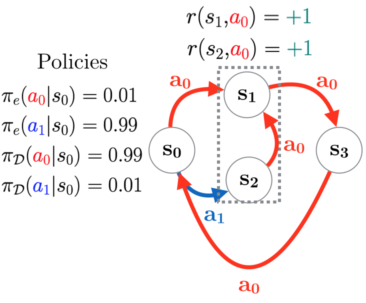
(a) Assumption 2 (transition dynamics) violated

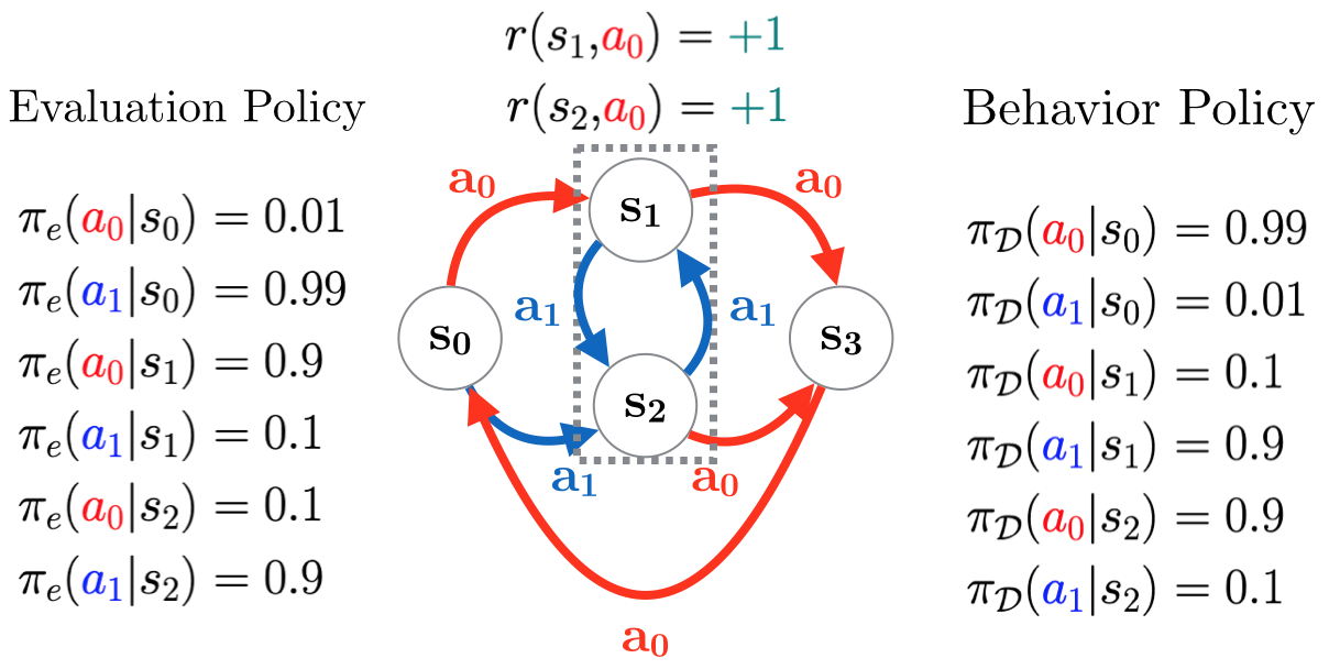
(b) Assumption 3 ($\pi_{e}$ action equality) violated

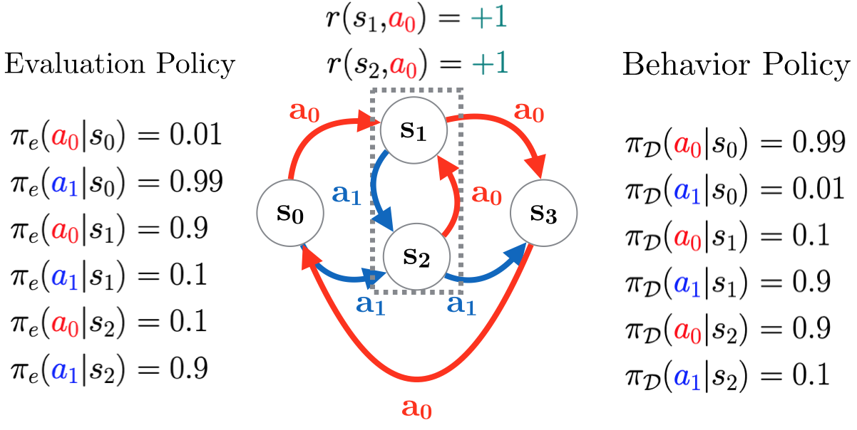
(c) Assumptions 2 and 3 violated. ($a_{0}$ and $a_{1}$ in $s_{2}$ switched)

Figure 6: Variations to the TwoPath MDP from Figure 2 to violate assumptions.

In practice, Assumptions 2 and 3 may be hard to validate. To study the impact of violation of these assumptions, we consider the following variations (Figure 6) to the original TwoPath MDP presented in Figure 2. In all these MDPS, we only aggregate $s_{1}$ and $s_{2}$. The policies in the last two MDPs are the same. Figure 7 illustrates the accuracy of AbstractBestDICE’s true ratio estimation. In general, we do see AbstractBestDICE fails to compute the true abstract ratios when these assumptions are violated.

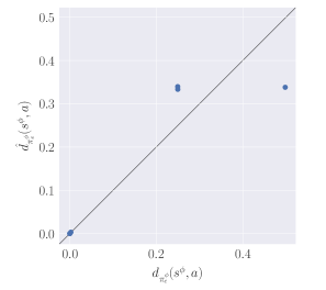
(a) Assumption 2 (transition dynamics) violated

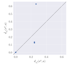
(b) Assumption 3 ($\pi_{e}$ action equality) violated

(c) Assumptions 2 and 3 violated

Figure 7: True ratio estimations with assumption violations. Closer to the linear line is better.

A.6 Additional Function Approximation Experiments and Details

Oracle $\rho(\pi_{e})$ Values

On each domain, we executed $\pi_{e}$ for $200$ episodes and averaged the results.

Policies

For each of the domains, we used the following policies:

• Reacher: We trained a policy using PPO (Schulman et al. 2017). $\pi_{e}$ was the trained policy after $100$k time-steps with a standard deviation of $0.1$ on the action dimensions while $\pi_{b}$ used $0.5$ as the standard deviation.

• Walker2D: We trained a policy using PPO (Schulman et al. 2017). $\pi_{e}$ was the trained policy after $100$k time-steps with a standard deviation of $0.1$ on the action dimensions while $\pi_{b}$ used $0.5$ as the standard deviation.

• Pusher: We trained a policy using PPO (Schulman et al. 2017). $\pi_{e}$ was the trained policy after $100$k time-steps with a standard deviation of $0.1$ on the action dimensions while $\pi_{b}$ used $0.5$ as the standard deviation.

• AntUMaze: We used the policies made available (Fu et al. 2021). $\pi_{e}$ was the final 10th snapshot saved and $\pi_{b}$ was the 5th snapshot. Each also had $0.1$ standard deviation on the action dimensions.

Trajectory Length

For each of the domains, the trajectory length is: $200$ for Reacher, $500$ for Walker2D, $300$ for Pusher, and $500$ for AntUMaze.

Hyperparameters

For BestDICE and AbstractBestDICE, we fixed the following hyperparameters:

• $\gamma=0.995$ in all experiments.

• Neural net architecture: All neural networks are $2$ layers with $64$ hidden units using tanh activation.

• Unit mean constraint learning rate (Zhang, Liu, and Whiteson 2020; Yang et al. 2020): $\lambda=1e^{-3}$.

• Optimizer: Adam optimizer with default parameters in Pytorch.

• Positivity constraint: squaring function on the last layer of the neural network.

We conducted a search for the learning rate of $\nu$ ($\alpha_{\nu})$ and learning rate of $\zeta$ ($\alpha_{\zeta}$), . The learning rate search for ($\alpha_{\nu},\alpha_{\zeta}$) was over $\{(5e^{-5},5e^{-5}),(1e^{-4},1e^{-4}),(3e^{-4},3e^{-4}),(7e^{-4},7e^{-4}),(1e^{-3},1e^{-3})\}$. The optimal hyperparameters ($\alpha_{\nu}=\alpha_{\zeta}$) for each environment and batch size were:

	5	10	50	75	100	300	500	1000
Reacher	$5e^{-5}$	$1e^{-4}$	$1e^{-3}$	$1e^{-4}$	$1e^{-4}$	$7e^{-4}$	$1e^{-3}$	$7e^{-4}$
Walker2D	$1e^{-3}$	$5e^{-5}$	$5e^{-5}$	$5e^{-5}$	$5e^{-5}$	$5e^{-5}$	$5e^{-5}$	$5e^{-5}$
Pusher	$5e^{-5}$	$5e^{-5}$	$5e^{-5}$	$5e^{-5}$	$1e^{-4}$	$5e^{-5}$	$5e^{-5}$	$5e^{-5}$
AntUMaze	$3e^{-4}$	$5e^{-5}$	$5e^{-5}$	$5e^{-5}$	$5e^{-5}$	$5e^{-5}$	$5e^{-5}$	$5e^{-5}$

Table 1: Optimal hyparameters for AbstractBestDICE on each batch size and environment.

	5	10	50	75	100	300	500	1000
Reacher	$5e^{-5}$	$1e^{-4}$	$5e^{-5}$	$1e^{-4}$	$5e^{-5}$	$1e^{-4}$	$3e^{-4}$	$1e^{-3}$
Walker2D	$5e^{-5}$	$3e^{-4}$	$7e^{-4}$	$7e^{-4}$	$7e^{-4}$	$1e^{-4}$	$3e^{-4}$	$1e^{-4}$
Pusher	$5e^{-5}$	$1e^{-4}$	$1e^{-4}$	$5e^{-5}$	$1e^{-4}$	$5e^{-5}$	$1e^{-4}$	$5e^{-5}$
AntUMaze	$1e^{-4}$	$3e^{-4}$	$5e^{-5}$	$5e^{-5}$	$5e^{-5}$	$5e^{-5}$	$5e^{-5}$	$5e^{-5}$

Table 2: Optimal hyperparameters for BestDICE on each batch size and environment.

Empirical Estimator

In practice we use a weighted importance sampling (Yang et al. 2020) approach for the function approximation cases to estimate $\rho(\pi_{e})$ (same for BestDICE):

$$\hat{\rho}(\pi^{\phi}_{e}) =\frac{\sum_{i=1}^{N}\frac{d_{\pi^{\phi}_{e}}(s_{i}^{\phi},a_{i})}{d_{\pi^{\phi}_{\mathcal{D}}}(s_{i}^{\phi},a_{i})}r^{\phi}(s_{i}^{\phi},a_{i})}{\sum_{i=1}^{N}\frac{d_{\pi^{\phi}_{e}}(s_{i}^{\phi},a_{i})}{d_{\pi^{\phi}_{\mathcal{D}}}(s_{i}^{\phi},a_{i})}}$$

Misc Abstraction Details

• For Walker2D, we modified the default reward function from incremental distance covered at each time-step to distance from start location at each time-step to ensure Assumption 1 is satisfied.

• For AntUMaze, the reward function is originally $r(s^{\prime})$ i.e. it is based on the next state that the ant moves to. To ensure Assumption 1 is satisfied, we changed this reward function to be of the current state, $r(s)$.

Additional Results

Baseline Performance Comparison As also reported by Yang et al. (2020); Fu et al. (2021), we found in preliminary experiments that BestDICE performed much better than other MIS methods such as DualDICE (Nachum et al. 2019), Minimax-Weight Learning (Uehara, Huang, and Jiang 2019), etc.

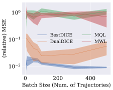
(a) Reacher

(b) Walker

Figure 8: Baseline Performance comparison among common MIS methods (after hyperparameter search). Lower is better.

Additional Hyperparameter Robustness Results In general, we can see AbstractBestDICE can be much more robust than BestDICE to hyperparameter tuning.

(a) Reacher (Batch size: 5)

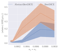
(b) Reacher (Batch size: 10)

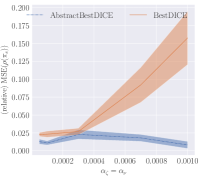
(c) Reacher (Batch size: 50)

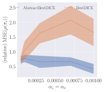
(d) Walker2D (Batch size: 5)

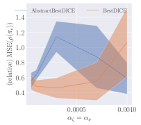
(e) Walker2D (Batch size: 10)

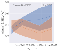
(f) Walker2D (Batch size: 50)

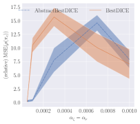
(g) Pusher (Batch size: 5)

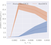
(h) Pusher (Batch size: 10)

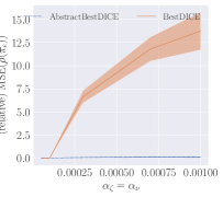
(i) Pusher (Batch size: 50)

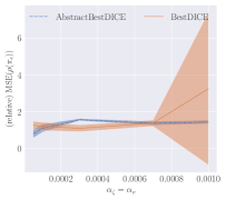
(j) AntUMaze (Batch size: 10)

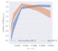
(k) AntUMaze (Batch size: 50)

Figure 9: Hyperparameter sensitivity graph for BestDICE and AbstractBestDICE. $\alpha_{\zeta}=\alpha_{\nu}$ Errors are computed over $15$ trials with $95\%$ confidence intervals. Lower is better. Pusher for batch size of $50$ is shown in the main paper.

Training Stability In Figure 10 we show that $\phi$ can improve training stability.

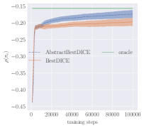
(a) Reacher (Batch size: 10)

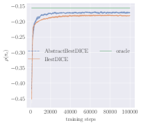
(b) Reacher (Batch size: 500)

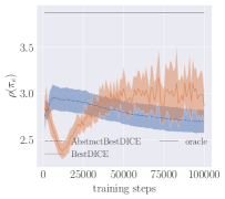
(c) Walker2D (Batch size: 10)

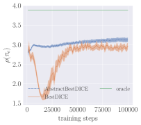
(d) Walker2D (Batch size: 500)

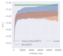
(e) Pusher (Batch size: 10)

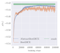
(f) Pusher (Batch size: 500)

(g) AntUMaze (Batch size: 10)

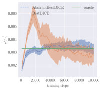
(h) AntUMaze (Batch size: 500)

Figure 10: Reward vs. Training Steps. Errors are computed over $15$ trials with $95\%$ confidence intervals. These figures illustrate the training stability of AbstractBestDICE over BestDICE. Lower is better.

Abstract Quality and Data-Efficiency. We find that not all abstractions that satisfy Assumption 1 lead to better performance. For example, the following are valid abstractions on the Reacher task: 1) the Euclidean distance between the arm and goal, $s^{\phi}\in\mathbb{R}$ and the 3D vector between the arm and goal, $s^{\phi}\in\mathbb{R}^{3}$ (Figure 11). However, in practice we found that these were unreliable. One possible reason for this unreliability is that these abstractions are incredibly extreme and the algorithm may be unable to differentiate between abstract state, resulting in outputting similar $\zeta^{\phi}(s^{\phi},a)\forall s^{\phi}$.

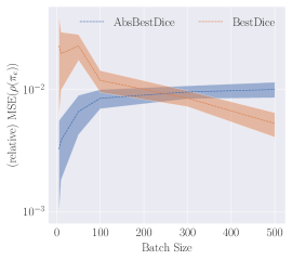
(a) Reacher

Figure 11: Relative MSE vs. Batch Size. $y$ axis is log-scaled. Errors are computed over $15$ trials with $95\%$ confidence intervals. This figures illustrate valid abstractions can be more data-inefficient than the ground equivalents. Lower is better.

A.7 Hardware For Experiments

• Distributed cluster on HTCondor framework

• Intel(R) Xeon(R) CPU E5-2470 0 @ 2.30GHz

• RAM: 5GB

• Disk space: 4GB

References

- Abel (2020) Abel, D. 2020. A Theory of Abstraction in Reinforcement Learning. Ph.D. thesis, Brown University.
- Brockman et al. (2016) Brockman, G.; Cheung, V.; Pettersson, L.; Schneider, J.; Schulman, J.; Tang, J.; and Zaremba, W. 2016. OpenAI Gym. CoRR, abs/1606.01540.
- Castro (2020) Castro, P. S. 2020. Scalable Methods for Computing State Similarity in Deterministic Markov Decision Processes. Proceedings of the AAAI Conference on Artificial Intelligence, 34(06): 10069–10076.
- Chen and Jiang (2022) Chen, J.; and Jiang, N. 2022. Offline Reinforcement Learning Under Value and Density-Ratio Realizability: The Power of Gaps. In The 38th Conference on Uncertainty in Artificial Intelligence.
- Dai et al. (2016) Dai, B.; He, N.; Pan, Y.; Boots, B.; and Song, L. 2016. Learning from Conditional Distributions via Dual Kernel Embeddings. CoRR, abs/1607.04579.
- Dietterich (1999) Dietterich, T. G. 1999. Hierarchical Reinforcement Learning with the MAXQ Value Function Decomposition.
- Ferns, Panangaden, and Precup (2011) Ferns, N.; Panangaden, P.; and Precup, D. 2011. Bisimulation Metrics for Continuous Markov Decision Processes. SIAM Journal on Computing, 40(6): 1662–1714.
- Fu et al. (2020) Fu, J.; Kumar, A.; Nachum, O.; Tucker, G.; and Levine, S. 2020. D4RL: Datasets for Deep Data-Driven Reinforcement Learning. arXiv:2004.07219.
- Fu et al. (2021) Fu, J.; Norouzi, M.; Nachum, O.; Tucker, G.; Wang, Z.; Novikov, A.; Yang, M.; Zhang, M. R.; Chen, Y.; Kumar, A.; Paduraru, C.; Levine, S.; and Paine, T. 2021. Benchmarks for Deep Off-Policy Evaluation. In ICLR.
- Gelada and Bellemare (2019) Gelada, C.; and Bellemare, M. G. 2019. Off-Policy Deep Reinforcement Learning by Bootstrapping the Covariate Shift. Proceedings of the AAAI Conference on Artificial Intelligence, 33(01): 3647–3655.
- Gelada et al. (2019) Gelada, C.; Kumar, S.; Buckman, J.; Nachum, O.; and Bellemare, M. G. 2019. DeepMDP: Learning Continuous Latent Space Models for Representation Learning. CoRR, abs/1906.02736.
- Geng et al. (2022) Geng, X.; Li, K.; Gupta, A.; Kumar, A.; and Levine, S. 2022. Effective Offline RL Needs Going Beyond Pessimism: Representations and Distributional Shift. In Decision Awareness in Reinforcement Learning Workshop at ICML 2022.
- Hallak and Mannor (2017) Hallak, A.; and Mannor, S. 2017. Consistent On-Line Off-Policy Evaluation.
- Hanna, Niekum, and Stone (2019) Hanna, J.; Niekum, S.; and Stone, P. 2019. Importance Sampling Policy Evaluation with an Estimated Behavior Policy. In Proceedings of the 36th International Conference on Machine Learning (ICML).
- Hanna, Stone, and Niekum (2017) Hanna, J.; Stone, P.; and Niekum, S. 2017. Bootstrapping with Models: Confidence Intervals for Off-Policy Evaluation. In Proceedings of the 16th International Conference on Autonomous Agents and Multiagent Systems (AAMAS).
- Jiang and Li (2015) Jiang, N.; and Li, L. 2015. Doubly Robust Off-policy Value Evaluation for Reinforcement Learning.
- Le, Voloshin, and Yue (2019) Le, H. M.; Voloshin, C.; and Yue, Y. 2019. Batch Policy Learning under Constraints.
- Li, Walsh, and Littman (2006) Li, L.; Walsh, T. J.; and Littman, M. L. 2006. Towards a Unified Theory of State Abstraction for MDPs. In In Proceedings of the Ninth International Symposium on Artificial Intelligence and Mathematics, 531–539.
- Liu et al. (2018a) Liu, Q.; Li, L.; Tang, Z.; and Zhou, D. 2018a. Breaking the Curse of Horizon: Infinite-Horizon Off-Policy Estimation. CoRR, abs/1810.12429.
- Liu, Bacon, and Brunskill (2019) Liu, Y.; Bacon, P.-L.; and Brunskill, E. 2019. Understanding the Curse of Horizon in Off-Policy Evaluation via Conditional Importance Sampling.
- Liu et al. (2018b) Liu, Y.; Gottesman, O.; Raghu, A.; Komorowski, M.; Faisal, A.; Doshi-Velez, F.; and Brunskill, E. 2018b. Representation Balancing MDPs for Off-Policy Policy Evaluation.
- Nachum et al. (2019) Nachum, O.; Chow, Y.; Dai, B.; and Li, L. 2019. DualDICE: Behavior-Agnostic Estimation of Discounted Stationary Distribution Corrections. In Advances in Neural Information Processing Systems, volume 32. Curran Associates, Inc.
- Paine et al. (2020) Paine, T. L.; Paduraru, C.; Michi, A.; Gülçehre, Ç.; Zolna, K.; Novikov, A.; Wang, Z.; and de Freitas, N. 2020. Hyperparameter Selection for Offline Reinforcement Learning. CoRR, abs/2007.09055.
- Precup, Sutton, and Singh (2000) Precup, D.; Sutton, R. S.; and Singh, S. P. 2000. Eligibility Traces for Off-Policy Policy Evaluation. In Proceedings of the Seventeenth International Conference on Machine Learning, ICML ’00, 759–766. San Francisco, CA, USA: Morgan Kaufmann Publishers Inc. ISBN 1558607072.
- Rockafellar and Wets (1998) Rockafellar, R.; and Wets, R. J.-B. 1998. Variational Analysis. Heidelberg, Berlin, New York: Springer Verlag.
- Rockafellar (1970) Rockafellar, R. T. 1970. Convex analysis. Princeton Mathematical Series. Princeton, N. J.: Princeton University Press.
- Schulman et al. (2017) Schulman, J.; Wolski, F.; Dhariwal, P.; Radford, A.; and Klimov, O. 2017. Proximal Policy Optimization Algorithms. CoRR, abs/1707.06347.
- Singh, Jaakkola, and Jordan (1994) Singh, S.; Jaakkola, T.; and Jordan, M. 1994. Reinforcement Learning with Soft State Aggregation. In Tesauro, G.; Touretzky, D.; and Leen, T., eds., Advances in Neural Information Processing Systems, volume 7. MIT Press.
- Sutton and Barto (2018) Sutton, R. S.; and Barto, A. G. 2018. Reinforcement Learning: An Introduction. The MIT Press, second edition.
- Sutton et al. (2008) Sutton, R. S.; Szepesvári, C.; Geramifard, A.; and Bowling, M. 2008. Dyna-Style Planning with Linear Function Approximation and Prioritized Sweeping. In Proceedings of the Twenty-Fourth Conference on Uncertainty in Artificial Intelligence, UAI’08, 528–536. Arlington, Virginia, USA: AUAI Press. ISBN 0974903949.
- Thomas, Theocharous, and Ghavamzadeh (2015) Thomas, P.; Theocharous, G.; and Ghavamzadeh, M. 2015. High-Confidence Off-Policy Evaluation. Proceedings of the AAAI Conference on Artificial Intelligence, 29(1).
- Thomas (2015) Thomas, P. S. 2015. Safe Reinforcement Learning. Ph.D. thesis, University of Massachusetts Amherst.
- Thomas and Brunskill (2016) Thomas, P. S.; and Brunskill, E. 2016. Data-Efficient Off-Policy Policy Evaluation for Reinforcement Learning. arXiv:1604.00923.
- Uehara, Huang, and Jiang (2019) Uehara, M.; Huang, J.; and Jiang, N. 2019. Minimax Weight and Q-Function Learning for Off-Policy Evaluation.
- Voloshin et al. (2021) Voloshin, C.; Le, H. M.; Jiang, N.; and Yue, Y. 2021. Empirical Study of Off-Policy Policy Evaluation for Reinforcement Learning. In Thirty-fifth Conference on Neural Information Processing Systems Datasets and Benchmarks Track (Round 1).
- Wang et al. (2021) Wang, R.; Wu, Y.; Salakhutdinov, R.; and Kakade, S. M. 2021. Instabilities of Offline RL with Pre-Trained Neural Representation.
- Wen et al. (2020) Wen, J.; Dai, B.; Li, L.; and Schuurmans, D. 2020. Batch Stationary Distribution Estimation. In Proceedings of the 37th International Conference on Machine Learning, ICML’20. JMLR.org.
- Xie, Ma, and Wang (2019) Xie, T.; Ma, Y.; and Wang, Y.-X. 2019. Towards Optimal Off-Policy Evaluation for Reinforcement Learning with Marginalized Importance Sampling. In Advances in Neural Information Processing Systems, volume 32. Curran Associates, Inc.
- Yang et al. (2020) Yang, M.; Nachum, O.; Dai, B.; Li, L.; and Schuurmans, D. 2020. Off-Policy Evaluation via the Regularized Lagrangian. In Larochelle, H.; Ranzato, M.; Hadsell, R.; Balcan, M.; and Lin, H., eds., Advances in Neural Information Processing Systems, volume 33, 6551–6561. Curran Associates, Inc.
- Yin et al. (2022) Yin, M.; Duan, Y.; Wang, M.; and Wang, Y.-X. 2022. Near-optimal Offline Reinforcement Learning with Linear Representation: Leveraging Variance Information with Pessimism.
- Yin and Wang (2020) Yin, M.; and Wang, Y. 2020. Asymptotically Efficient Off-Policy Evaluation for Tabular Reinforcement Learning. CoRR, abs/2001.10742.
- Zhan et al. (2022) Zhan, W.; Huang, B.; Huang, A.; Jiang, N.; and Lee, J. 2022. Offline Reinforcement Learning with Realizability and Single-policy Concentrability. In Loh, P.-L.; and Raginsky, M., eds., Proceedings of Thirty Fifth Conference on Learning Theory, volume 178 of Proceedings of Machine Learning Research, 2730–2775. PMLR.
- Zhang et al. (2021a) Zhang, A.; McAllister, R. T.; Calandra, R.; Gal, Y.; and Levine, S. 2021a. Learning Invariant Representations for Reinforcement Learning without Reconstruction. In International Conference on Learning Representations.
- Zhang et al. (2021b) Zhang, M. R.; Paine, T.; Nachum, O.; Paduraru, C.; Tucker, G.; ziyu wang; and Norouzi, M. 2021b. Autoregressive Dynamics Models for Offline Policy Evaluation and Optimization. In International Conference on Learning Representations.
- Zhang et al. (2020) Zhang, R.; Dai, B.; Li, L.; and Schuurmans, D. 2020. GenDICE: Generalized Offline Estimation of Stationary Values.
- Zhang, Liu, and Whiteson (2020) Zhang, S.; Liu, B.; and Whiteson, S. 2020. GradientDICE: Rethinking Generalized Offline Estimation of Stationary Values. In III, H. D.; and Singh, A., eds., Proceedings of the 37th International Conference on Machine Learning, volume 119 of Proceedings of Machine Learning Research, 11194–11203. PMLR.