Joint Hybrid Delay-Phase Precoding Under True-Time Delay Constraints in Wideband THz Massive MIMO Systems

Abstract

The beam squint effect that arises in the wideband Terahertz (THz) massive multiple-input multiple-output (MIMO) communication produces a serious array gain loss. True-time delay (TTD)-based hybrid precoding has been considered to compensate for the beam squint effect. By fixing the phase shifter (PS) precoder, a common strategy has been designing TTD precoder under the assumption of unbounded time delay values. In this paper, we present a new approach to the problem of beam squint compensation, based on the joint optimization of the TTD and PS precoders under per TTD device time delay constraints. We first derive a lower bound of the achievable rate. Then, we show that in the large system limit, the ideal analog precoder that completely compensates for the beam squint is equivalent to the one that maximizes the achievable rate lower bound. Unlike the prior approaches, our approach does not require the unbounded time delay assumption; the range of time delay values that a TTD can produce is strictly limited in our approach. Instead of focusing on the design of TTD values only, we jointly optimize both the TTD and PS values to effectively cope with the practical time delay constraints. Taking the advantage of the proposed joint TTD and PS precoder optimization approach, we quantify the minimum number of TTDs required to produce a predefined array gain performance. The simulation results illustrate the substantially improved performance with the array gain performance guarantee of the proposed joint optimization method.

I Introduction

The fifth generation (5G)-&-beyond wireless systems are expected to support many new high data rate applications such as augmented reality/virtual reality (AR/VR), eHeath, and holographic telepresence [2]. To facilitate the proposed usecases, communications in the terahertz (THz) band (0.1-10 THz) have recently attracted significant interests from both acamedia and industry because of an abundance of wideband spectrum resources [3, 4, 5]; compare to the current millimeter-wave (mmWave) communications in the 5G specifications [6] that utilize a few gigahertz (GHz) bandwidth, the THz communications [3, 4, 5] utilize tens of GHz bandwidth. Intriguingly, the data rates on the orders of 10 to 100 Gbps can be achieved using the currently available digital modulation techniques in THz frequencies [5, 7]. However, the envisioned THz communications face numerous challenges due to the high path losses, large power consumption, and inter-symbol interference. To deal with these challenges, the combination of hybrid massive multiple-input multiple-output (MIMO) and orthogonal frequency division multiplexing (OFDM) technologies has been popularly discussed [8, 9, 10, 11] recently.

It is well known that as the number of antennas grows, the MIMO system can be greatly simplified in terms of beamforming and precoding [12]. In view of this, strong theoretical analyses have justified the use of a very large number of antennas at the base station [12, 13, 14]. This has raised a significant interest in massive MIMO systems at sub-$6$GHz [12, 14, 13] and mmWave frequencies [15, 16, 17]. The underlying assumption behind the works in [12, 14, 13, 15, 16, 17] was, however, narrowband. Unlike the narrowband systems, wideband high-frequency massive MIMO OFDM systems may suffer from the substantial array gain loss across different OFDM subcarriers as the number of antennas grows due to the spatial-frequency wideband effect [18, 19, 20, 21], which is also known as the beam squint effect. In particular, beam squint refers to a phenomenon in which the deviation occurs in the spatial direction of each OFDM subcarrier when the wideband OFDM is used in a very large antenna array system. The implication of beam squint is that it causes a serious achievable rate degradation, which potentially demotivates the use of OFDM in the wideband THz massive MIMO systems. Therefore, an efficient beam squint compensation is of paramount importance for the realization of wideband THz massive MIMO communications.

I-A Related Works

The beam squint was previously addressed in wideband mmWave massive MIMO [18, 22] by designing the beamforming weights to produce adaptive-beamwidth beams in order to cover the squinted angles. While they show efficacy, these techniques cannot be directly extended to the THz bands due to the extremely narrow pencil beam requirement imposed by one or two orders of magnitude higher carrier frequencies. In the radar community, the beam squint effect of phased array antennas has been independently studied (e.g., see [23, 24, 25], and references therein). A common method to relieve the beam squint in radar is to employ the true-time delay (TTD) lines instead of using phase shifters (PSs) for analog beamforming [23, 24, 25]. In contrast with the PS-based analog beamforming that produces frequency-independent phase rotations, the TTD-based analog beamforming generates frequency-dependent phase rotations that can be used for correcting the squinted beams in the spatial domain. However, this method has limitation to be directly used in the massive MIMO systems because it requires a large number of TTD lines. Particularly, each transmit antenna needs to be fed by a dedicated TTD, leading to a high hardware cost and huge power consumption

Recently, there has been considerable interest in adopting TTD lines to THz hybrid massive MIMO OFDM systems to cope with beam squint [8, 9, 10]. Compared with the conventional TTD-based beamforming architectures in radar [23, 24, 25], these systems [8, 9, 10] employ a substantially lower number of TTD lines to maintain their power consumption as low as possible; one can think of these methods as combining a small number of TTD lines with a layer of PSs to form an analog precoder so that the capability of generating frequency-dependent phase rotations is maintained while consuming less power than the conventional TTD architecture in radar systems. Nevertheless, these approaches may still suffer from a large amount of power consumption when a large number of TTD lines is required to combat with the extremely severe beam squint present in the wideband THz massive MIMO OFDM systems. Especially, the question of how to quantify the number of TTDs per RF chain to produce a desired beam squint compensation capability remains challenging.

More recently, the TTD-based hybrid precoding architecture has been exploited to solve fast beam training [28], beam tracking [29], and user localization [30] problems. In contrary with the beam squint compensation that focuses the beam directions at every OFDM subcarrier to the same physical direction, these works [28, 29, 30] take advantage of the beam squint effect by spreading the beams across different OFDM subcarriers simultaneously. By doing so, information such as users’ physical locations in different directions can be tracked simultaneously [30].

Most of these prior works have focused on the design of the TTD precoder while fixing the PS precoder, in which the analog precoding design is simplified because it decouples the TTD and PS precoders; the number of design variables is substantially reduced since the number of deployed TTDs is much less than the number of PSs. Furthermore, it was assumed that the TTD values increase linearly with the number of antennas without bounds. In practice, it is difficult to implement these approaches because the unbounded TTD assumption cannot be realizable. The range of time delay values that a TTD can produce is strictly limited (e.g., $\leq 508$ ps [26]). Hence, to cope with the practical constraints of TTD, it is much desirable to jointly optimize both the TTD and PS precoders.

I-B Overview of Contributions

Motivated by the preceding discussion, we present a joint TTD and PS optimization methodology to mitigate the beam squint effect. The practical TTD constraint is forced where the time delay values are restricted in a given interval. The major contributions of this paper are summarized as follows.

• We approach the general TTD-based hybrid precoder design in the wideband THz massive MIMO OFDM system from an achievable-rate-maximization point of view to present the impact of compensating the beam squint on the achievable rate performance. Treating the product of TTD and PS precoders as a composite analog precoder, we first derive a lower bound of the achievable rate and show that in the large system limit the ideal analog precoder that completely compensates for the beam squint is equivalent to the one that maximizes the achievable rate lower bound.

• Provided the ideal analog precoder identified, we formulate the joint TTD and PS precoder optimization problem based on minimizing the distance between the ideal analog precoder and the product of TTD and PS precoders under the TTD constraints. In contrast with the prior approaches [8, 9, 10] that only optimize the TTD precoder and assume the unbounded time delay values, we jointly optimize the TTD and PS precoders and the range of time delay values that a TTD can produce in our approach is strictly limited. Although the formulated problem is non-convex and difficult to solve directly, we show that by transforming the problem into the phase domain, the original problem is converted to an equivalent convex problem, which allows us to find a closed form of the global optimal solution. On the basis of the identified optimal solution, our analysis reveals the number of transmit antennas and the amount of time delay required for the best beam squint compensation of our method.

• Leveraging the advantages of the closed-form expressions of our proposed joint optimization approach, a mixed-integer optimization problem is formulated to quantify the minimum number of TTDs required to achieve a predefined array gain performance. Although the formulated mixed-integer problem is intractable, we show that by applying a second-order approximation, the original problem can be relaxed to a tractable form, which enables us to find an optimal solution. Our analysis reveals that when the number of OFDM subcarriers grows, the number of TTDs is linearly increasing with respect to the system bandwidth in order to guarantee a required array gain performance at every OFDM subcarrier.

• We carry out extensive simulations to evaluate the performance of the proposed joint PS and TTD precoding. The simulation results verify that with our optimal design, the beam squint is compensated effectively. Through the simulations, our joint optimization approach outperforms the prior TTD-based precoding approaches that only optimize TTD precoder in terms of array gain and achievable rate. The simulations verify the substantial array gain performance improvement with the minimum number of TTDs informed by our optimization approaches.

Synopsis: The remainder of the paper is organized as follows. Section II presents the channel models of the wideband THz massive MIMO OFDM system and analyzes the array gain loss caused by the beam squint. Section III describes the relationship between beam squint compensation by the ideal analog precoder and the achievable rate lower bound. Then, Section IV derives the closed-form solution of the optimal TTD and PS precoders under the practical TTD constraints and quantifies the minimum number of TTDs that ensures a predefined array gain performance. Section V provides simulation results to corroborate the developed analysis. Finally, the conclusion of this work is drawn in Section VI.

Notation: A bold lower case letter ${\mathbf{x}}$ is a column vector and a bold upper case letter ${\mathbf{X}}$ is a matrix. ${\mathbf{X}}^{T}$, ${\mathbf{X}}^{H}$, $\|{\mathbf{X}}\|_{F}$, $\mathop{\mathrm{tr}}({\mathbf{X}})$, $\mathop{\mathrm{det}}({\mathbf{X}})$, ${\mathbf{X}}(i,j)$, $\|{\mathbf{x}}\|_{2}$, $|x|$, and $\otimes$ are, respectively, the transpose, conjugate transpose, Frobenius norm, trace, determinant, $i$th row and $j$th column entry of ${\mathbf{X}}$, $2$-norm of ${\mathbf{x}}$, modulus of $x\in{\mathbb{C}}$, and Kronecker product. $\mathop{\mathrm{blk}}({\mathbf{x}}_{1},{\mathbf{x}}_{2},\dots,{\mathbf{x}}_{N})$ is an $nN\times N$ block diagonal matrix such that its main-diagonal blocks contain ${\mathbf{x}}_{i}\in{\mathbb{C}}^{n\times 1}$, for $i=1,2,\dots,N$ and all off-diagonal blocks are zero. $\mathbf{0}_{n}$, $\mathbf{1}_{n}$, and ${\mathbf{I}}_{n}$ denote, respectively, the $n\times 1$ all-zero vector, $n\times 1$ all-one vector, and $n\times n$ identity matrix. Given ${\mathbf{x}}\in{\mathbb{R}}^{n\times 1}$, $e^{j{\mathbf{x}}}$ denotes the column vector $[e^{jx_{1}}~{}e^{jx_{2}}~{}\dots~{}e^{jx_{n}}]^{T}\in{\mathbb{C}}^{n\times 1}$ obtained by applying $e^{j}$ element-wise.

II Channel Model and Beam Squint Effect

In this section, we present the channel model of the wideband THz massive MIMO OFDM systems. Then, the array gain loss caused by the beam squint is analyzed.

II-A Channel Model

We consider the downlink of a wideband THz hybrid massive MIMO OFDM system where the transmitter is equipped with an $N_{t}$-element transmit antenna array with element spacing $d$. The transmit antenna array is fed by $N_{RF}$ radio frequency (RF) chains to simultaneously transmit $N_{s}$ data streams to an $N_{r}$-antenna receiver. It is assumed that $N_{t},N_{r},N_{RF},$ and $N_{s}$ satisfy $N_{s}=N_{RF}=N_{r}\ll N_{t}$. Herein, we let $f_{c}$, $B$, and $K$ be, respectively, the central (carrier) frequency, bandwidth of the OFDM system, and the number of OFDM subcarriers (an odd number). Then, the $k$th subcarrier frequency is given by

$$f_{k}=f_{c}+\frac{B}{K}\Big{(}k-1-\frac{K-1}{2}\Big{)},~{}\text{for}~{}k=1,2,\dots,K.$$ (1)

The frequency domain MIMO OFDM channel at the $k$th subcarrier ${\mathbf{H}}_{k}\in{\mathbb{C}}^{N_{r}\times N_{t}}$ is

$${\mathbf{H}}_{k}=\sqrt{\frac{N_{r}N_{t}}{L}}\sum_{l=1}^{L}\alpha_{l}e^{-j2\pi\tau_{l}f_{k}}{\mathbf{u}}_{k,l}{\mathbf{v}}^{H}_{k,l},$$ (2)

where $L$ denotes the number of channel (spatial) paths, and $\alpha_{l}\in{\mathbb{C}}$ and $\tau_{l}\in{\mathbb{R}}$ represent the gain and delay of the $l$th path of the channel, respectively. For ease of exposition, we assume $L=N_{RF}$, which is equivalent to setting $\alpha_{l}=0$, $\forall l>N_{RF}$ in (2). In the remainder of this paper, we use the subscript $l$ for denoting the index of both channel path and RF chain unless specified otherwise. The vectors ${\mathbf{v}}_{k,l}\in{\mathbb{C}}^{N_{t}\times 1}$ and ${\mathbf{u}}_{k,l}\in{\mathbb{C}}^{N_{r}\times 1}$ in (2) are the normalized transmit and receive array response vectors of the $k$th subcarrier on the $l$th path, respectively, where the ${\mathbf{v}}_{k,l}$ is a function of angles of departure (AoDs), i.e., the transmit azimuth $\Psi_{l}\in[\Psi_{\min},\Psi_{\max}]$ and elevation $\overline{\Psi}_{l}\in[\overline{\Psi}_{\min},\overline{\Psi}_{\max}]$ angles, for $l=1,2,\dots,L$. The exactly same definition applies to the normalized receive array response vector ${\mathbf{u}}_{k,l}$ in (2).

In what follows, we will limit our discussion to the transmit antenna array, keeping in mind that the same applies to the receive array. The antenna geometry of the transmit array is described assuming far-field spatial angles. When the transmit antenna array is uniform rectangular array (URA) located on the $yz$-plane with $N_{1}$ and $N_{2}$ elements on the $y$ and $z$ axis, respectively, such that $N_{t}=N_{1}\times N_{2}$, the transmit array response vector ${\mathbf{v}}_{k,l}$ in (2) can be modeled by

$${\mathbf{v}}_{k,l}={\mathbf{v}}^{y}_{k,l}\otimes{\mathbf{v}}^{z}_{k,l},$$ (3)

where the $n_{1}$th entry of ${\mathbf{v}}^{y}_{k,l}\!\in\!{\mathbb{C}}^{N_{1}\times 1}$ is ${\mathbf{v}}^{y}_{k,l}(n_{1},1)\!=\!\frac{1}{\sqrt{N_{1}}}e^{-j\pi\frac{2df_{k}}{c}(n_{1}-1)\sin(\Psi_{l})\sin(\overline{\Psi}_{l})}$, for $n_{1}\!=\!1,2,\dots,N_{1}$, the $n_{2}$th entry of ${\mathbf{v}}^{z}_{k,l}\!\in\!{\mathbb{C}}^{N_{2}\times 1}$ is ${\mathbf{v}}^{z}_{k,l}(n_{2},1)\!=\!\frac{1}{\sqrt{N_{2}}}e^{-j\pi\frac{2df_{k}}{c}(n_{2}-1)\cos(\overline{\Psi}_{l})}$, for $n_{2}\!=\!1,2,\dots,N_{2}$, and $c\!=\!3\times 10^{8}$ m/s denotes the speed of light. In particular, ${\mathbf{v}}^{z}_{k,l}\!=\!\frac{1}{\sqrt{N_{2}}}\Big{[}1~{}\dots~{}e^{j\pi\frac{2df_{k}}{c}(N_{2}-1)\cos(\overline{\Psi}_{l})}\Big{]}^{H}$ and ${\mathbf{v}}^{y}_{k,l}\!=\!\frac{1}{\sqrt{N_{1}}}\Big{[}1~{}\dots~{}e^{j\pi\frac{2df_{k}}{c}(N_{1}-1)\sin(\Psi_{l})\sin(\overline{\Psi}_{l})}\Big{]}^{H}$. We define $\psi_{k,l}=\frac{2df_{k}}{c}\sin(\Psi_{l})\sin(\overline{\Psi}_{l})$ and $\overline{\psi}_{k,l}=\frac{2df_{k}}{c}\cos(\overline{\Psi}_{l})$ as the spatial directions of the $k$th subcarrier at the transmitter. Assuming the half wavelength antenna spacing, i.e., $d=\frac{c}{2f_{c}}$, the spatial directions at the central frequency are simplified to $\psi_{l}=\sin(\Psi_{l})\sin(\overline{\Psi}_{l})$ and $\overline{\psi}_{l}=\cos(\overline{\Psi}_{l})$. Hence, setting $\zeta_{k}=\frac{f_{k}}{f_{c}}$ leads to $\psi_{k,l}=\zeta_{k}\psi_{l}$, $\overline{\psi}_{k,l}=\zeta_{k}\overline{\psi}_{l}$, and

$$\zeta_{k}=1+\frac{B}{f_{c}}\Big{(}\frac{k-1-\frac{K-1}{2}}{K}\Big{)},$$ (4)

for $k=1,2,\dots,K$ and $l=1,2,\dots,L$, where (4) follows from the definition of $f_{k}$ in (1). As a result, the ${\mathbf{v}}^{y}_{k,l}$ and ${\mathbf{v}}^{z}_{k,l}$ in (3) can be succinctly expressed as ${\mathbf{v}}^{y}_{k,l}=\frac{1}{\sqrt{N_{1}}}\Big{[}1~{}\dots~{}e^{j\pi(N_{1}-1)\psi_{k,l}}\Big{]}^{H}$ and ${\mathbf{v}}^{z}_{k,l}=\frac{1}{\sqrt{N_{2}}}\Big{[}1~{}\dots~{}e^{j\pi(N_{2}-1)\overline{\psi}_{k,l}}\Big{]}^{H}$, respectively.

Note that in the remainder of this paper, we only consider the azimuth angle and set the elevation angle to $\frac{\pi}{2}$ rad, such that we are focusing on receivers that are directly in front of the transmit array. This simplification sets the uniform linear array (ULA) at the transmitter with $N_{1}=N_{t}$, $N_{2}=1$, and $\psi_{l}=\sin(\Psi_{l})$, $\forall l$, which sees the array response vector ${\mathbf{v}}_{k,l}$ in (3) to be ${\mathbf{v}}_{k,l}\!=\!\frac{1}{\sqrt{N_{t}}}\!\Big{[}\!1~{}\dots~{}e^{j\pi(N_{t}-1)\psi_{k,l}}\Big{]}^{H}\!\!\!\in\!{\mathbb{C}}^{N_{t}\times 1}$. Although this simplification is applied for the ease of exposition, it is straightforward to carry the elevation angle through the following developments presented in the later part of the paper.

II-B Beam Squint Effect

As aforementioned in Section I, when the wideband OFDM is employed in a massive MIMO system, a substantial array gain loss at each subcarrier could occur due to beam squint. To quantify it, we focus on the $l$th path of the massive MIMO OFDM channel in (2). Denoting the frequency-independent beamforming vector matched to the transmit array response vector with the AoD $\Psi_{l}$ as ${\mathbf{f}}^{(l)}={\mathbf{v}}_{c,l}$ (i.e., array response vector at the central frequency $f_{c}$ on the $l$th path), the array gain at the $k$th subcarrier of the $l$th path is given by $g({\mathbf{f}}^{(l)},\psi_{k,l})=|{\mathbf{v}}^{H}_{k,l}{\mathbf{f}}^{(l)}|$, i.e.,

$$\!\!\!\!g({\mathbf{f}}^{(l)},\psi_{k,l})=\frac{1}{N_{t}}\bigg{|}\sum_{n=0}^{N_{t}-1}e^{jn\pi(\psi_{k,l}-\psi_{l})}\bigg{|}=\bigg{|}\frac{\sin(N_{t}\Delta_{k,l})}{N_{t}\sin(\Delta_{k,l})}\bigg{|},$$ (5)

where $\Delta_{k,l}=\frac{\pi}{2}(\psi_{k,l}-\psi_{l})$. It is not difficult to observe that at the central frequency, the array gain is $g({\mathbf{f}}^{(l)},\psi_{k,l})=1$ because $\lim_{x\rightarrow 0}\frac{\sin(N_{t}x)}{\sin(x)}=N_{t}$. However, when $f_{k}\neq f_{c}$, $\Delta_{k,l}$ deviates from $0$; the amount of deviation increases as $f_{k}$ approaches to $f_{1}$ or $f_{K}$. As a result, all subcarriers except for the central subcarrier suffer from the array gain loss. The implication in the spatial domain is that the beams at non-central subcarriers may completely split from the one generated at the central subcarrier.

The following proposition quantifies the asymptotic array gain loss as $N_{t}\rightarrow\infty$.

Proposition 1.

Suppose that $\psi_{k,l}$ is the spatial direction at the $k$th subcarrier ($f_{k}\neq f_{c}$) of the $l$th path. Then, the array gain in (5) converges to $0$ as $N_{t}$ tends to infinity, i.e., $g({\mathbf{f}}^{(l)},\psi_{k,l})\stackrel{{\scriptstyle\boldsymbol{\cdot}}}{{=}}0$, where $\stackrel{{\scriptstyle\boldsymbol{\cdot}}}{{=}}$ denotes the equality when $N_{t}\rightarrow\infty$.

Proof.

The array gain in (5) can be rewritten as $g({\mathbf{f}}^{(l)},\psi_{k,l})=\frac{1}{N_{t}}\Big{|}\frac{\sin(N_{t}\Delta_{k,l})}{\pi\Delta_{k,l}}\frac{\pi\Delta_{k,l}}{\sin(\Delta_{k,l})}\Big{|},$ where $\Delta_{k,l}\neq 0$ because $f_{k}\neq f_{c}$. The proposition follows from the definition of Dirac delta function $\frac{\sin{(N_{t}\Delta_{k,l})}}{\pi\Delta_{k,l}}\stackrel{{\scriptstyle\boldsymbol{\cdot}}}{{=}}\delta(\Delta_{k,l})$ [31], compliting the proof. ∎

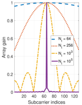
(a)

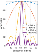
(b)

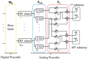
(c)

Figure 1: (a) Array gain vs. subcarrier indices for different numbers of transmit antennas ($N_{t}$). (b) Array gain vs. subcarrier indices for different bandwidths ($B$). (c) TTD-based hybrid precoding architecture

Fig. 1a illustrates the convergence trend of Proposition 1. The array gain patterns are calculated for $f_{c}=3$ THz, $K=129$, $\psi_{l}=0.8$, and $B=30$ GHz. As $N_{t}$ tends to be large, the maximum array gain is only achieved at the central frequency, i.e., $65$th subcarrier in Fig. 1a, while other subcarriers suffer from substantial array gain losses. This is quite opposite to the traditional narrowband massive MIMO system in which the array gain grows as $N_{t}\rightarrow\infty$.

The array gain loss is also numerically understood when the bandwidth $B$ increases. Fig. 1b illustrates those patterns when $B$ grows while using the same parameters as in Fig. 1a except for that $N_{t}=256$. As the bandwidth $B$ grows, the maximum array gain is obtained only at the central frequency while other subcarriers experience a large amount of array gain losses. This contrasts with the information-theoretic insight that the system achievable rate grows linearly with the bandwidth while keeping the signal-to-noise-ratio (SNR) fixed.

Wideband THz massive MIMO communication research is in its early stages. In order to truly unleash the potential of THz communications, a hybrid precoding architecture and methods that can effectively compensate for the beam squint effect under practical constraints is of paramount importance.

III Preliminaries and Achievable Rate Lower Bound

We consider a TTD-based hybrid precoding architecture [32, 9], where each RF chain drives $M$ TTDs and each TTD is connected to $N$ PSs as shown in Fig. 1c. The $N_{t}$-element ULA is divided into $M$ subarrays with $N=\frac{N_{t}}{M}$ antennas per subarray. The signal at the $k$th subcarrier passing through a TTD is delayed by $t$ ($0\leq t\leq t_{\max}$) in the time domain, which corresponds to the $-2\pi f_{k}t$ frequency-dependent phase rotation in the frequency domain. The $t_{\max}$ is the maximum time delay value that a TTD device can produce. The $k$th subcarrier signal at the receiver ${\mathbf{y}}_{k}\in{\mathbb{C}}^{N_{r}\times 1}$ is then given by [1]

$${\mathbf{y}}_{k}=\sqrt{\rho}{\mathbf{H}}_{k}{\mathbf{F}}_{1}{\mathbf{F}}_{2,k}(\{{\mathbf{t}}_{l}\}^{N_{RF}}_{l=1}){\mathbf{W}}_{k}{\mathbf{s}}_{k}+{\mathbf{n}}_{k},$$ (6)

where $\rho$, ${\mathbf{s}}_{k}\in{\mathbb{C}}^{N_{s}\times 1}$, ${\mathbf{W}}_{k}\in{\mathbb{C}}^{N_{RF}\times N_{s}}$, and ${\mathbf{n}}_{k}\in{\mathbb{C}}^{N_{r}\times 1}$ are, respectively, the average transmit power, transmit data stream, baseband digital precoder, and normal Gaussian noise vector with each entry being independent and identically distributed (i.i.d.) according to zero mean and variance $1$. The ${\mathbf{F}}_{1}$ in (6) is the PS precoding matrix, which is the concatenation of $N_{RF}$ PS submatrices ${\mathbf{X}}_{l}\in{\mathbb{C}}^{N_{t}\times M}$, $l=1,2,\dots,N_{RF}$, specifically,

$${\mathbf{F}}_{1}=\frac{1}{\sqrt{N_{t}}}[{\mathbf{X}}_{1}~{}{\mathbf{X}}_{2}~{}\dots~{}{\mathbf{X}}_{N_{RF}}]\in{\mathbb{C}}^{N_{t}\times MN_{RF}},\vspace{-0.2cm}$$ (7)

where ${\mathbf{X}}_{l}=\mathop{\mathrm{blk}}(e^{j\pi{\mathbf{x}}^{(l)}_{1}},e^{j\pi{\mathbf{x}}^{(l)}_{2}},\dots,e^{j\pi{\mathbf{x}}^{(l)}_{M}})\in{\mathbb{C}}^{N_{t}\times M}$, ${\mathbf{x}}^{(l)}_{m}=[x^{(l)}_{1,m}~{}x^{(l)}_{2,m}~{}\dots~{}x^{(l)}_{N,m}]^{T}\in{\mathbb{R}}^{N\times 1}$ is a PS vector, and $x^{(l)}_{n,m}$ is the value of the $n$th PS that is connected to the $m$th TTD on the $l$th RF chain, for $n=1,2\dots,N$, $l=1,2,\dots,N_{RF}$, and $m=1,2,\dots,M$. The ${\mathbf{F}}_{2,k}(\{{\mathbf{t}}_{l}\}^{N_{RF}}_{l=1})\in{\mathbb{C}}^{MN_{RF}\times N_{RF}}$ in (6) is the TTD precoding matrix, which is defined as

$$\!\!\!\!{\mathbf{F}}_{2,k}(\{{\mathbf{t}}_{l}\}^{N_{RF}}_{l=1})=\mathop{\mathrm{blk}}(e^{-j2\pi f_{k}{\mathbf{t}}_{1}},e^{-j2\pi f_{k}{\mathbf{t}}_{2}},\dots,e^{-j2\pi f_{k}{\mathbf{t}}_{N_{RF}}}),$$ (8)

where ${\mathbf{t}}_{l}=[t^{(l)}_{1}~{}t^{(l)}_{2}~{}\dots~{}t^{(l)}_{M}]^{T}\in{\mathbb{R}}^{M\times 1}$ is the $l$th time delay vector and $t^{(l)}_{m}$ is the time delay value of the $m$th TTD on the $l$th RF chain, for $m=1,2\dots,M$ and $l=1,2,\dots,N_{RF}$. For the ease of exposition, in what follows, we omit the time delay vectors $\{{\mathbf{t}}_{l}\}^{N_{RF}}_{l=1}$ in the TTD precoder notation ${\mathbf{F}}_{2,k}(\{{\mathbf{t}}_{l}\}^{N_{RF}}_{l=1})$, $\forall k$. We note that the analog precoder corresponds to the product ${\mathbf{F}}_{1}{\mathbf{F}}_{2,k}\in{\mathbb{C}}^{N_{t}\times N_{RF}}$ with the constant modulus constraint

$$|{\mathbf{F}}_{1}{\mathbf{F}}_{2,k}(i,j)|=\frac{1}{\sqrt{N_{t}}}\text{ and }{\mathbf{F}}_{1}{\mathbf{F}}_{2,k}\in{\mathcal{F}}_{N_{t},N_{RF}},\vspace{-0.1cm}$$ (9)

where ${\mathcal{F}}_{N_{t},N_{RF}}$ denotes the set of all matrices ${\mathbf{X}}\in{\mathbb{C}}^{N_{t}\times N_{RF}}$ such that $|{\mathbf{X}}(i,j)|=\frac{1}{\sqrt{N_{t}}},\forall i,j$. The data stream ${\mathbf{s}}_{k}$ in (6) satisfies $\mathbb{E}[{\mathbf{s}}_{k}{\mathbf{s}}^{H}_{k}]=\frac{1}{N_{s}}{\mathbf{I}}_{N_{s}}$. Then, the precoders are normalized such that $\|{\mathbf{F}}_{1}{\mathbf{F}}_{2,k}{\mathbf{W}}_{k}\|^{2}_{F}=N_{s}$, leading to

$$\mathbb{E}[\|{\mathbf{F}}_{1}{\mathbf{F}}_{2,k}{\mathbf{W}}_{k}{\mathbf{s}}_{k}\|^{2}_{2}]=1,~{}k=1,2,\dots,K.$$ (10)

III-A Preliminaries

We first describe the sign invariance property of the array gain in (5) and then identify the ideal analog precoder that completely compensates the beam squint. The sign invariance property and the ideal analog precoder established in this subsection will then be used in Section IV for jointly optimizing TTD and PS precoders.

III-A1 Sign Invariance of Array Gain

We define the combination of PS precoder ${\mathbf{F}}_{1}$ and TTD precoder ${\mathbf{F}}_{2,k}$ as

$${\mathbf{F}}_{k}={\mathbf{F}}_{1}{\mathbf{F}}_{2,k},\text{ for }k=1,2,\dots,K,$$ (11)

where the $l$th column of ${\mathbf{F}}_{k}$ is ${\mathbf{f}}^{(l)}_{k}=\frac{1}{\sqrt{N_{t}}}{\mathbf{X}}_{l}e^{-2\pi f_{k}{\mathbf{t}}_{l}}$, for $l=1,2,\dots,N_{RF}$. The array gain associated with ${\mathbf{f}}^{(l)}_{k}$ is then given, based on (5), by

$$\!\!\!\!\!\!\!\!g({\mathbf{f}}^{(l)}_{k},\psi_{k,l})=\frac{1}{N_{t}}\bigg{|}\sum\limits_{m=1}^{M}\sum\limits_{n=1}^{N}e^{j\pi\zeta_{k}\gamma^{(l)}_{n,m}}e^{j\pi x^{(l)}_{n,m}}e^{-j\pi\zeta_{k}\vartheta^{(l)}_{m}}\bigg{|},$$ (12)

where $\gamma^{(l)}_{n,m}=((m-1)N+n-1)\psi_{l}$ and $\vartheta^{(l)}_{m}=2f_{c}t^{(l)}_{m}\in[0,\vartheta_{\max}]$ with $\vartheta_{\max}=2f_{c}t_{\max}$. Note that in (12), $e^{j\pi\zeta_{k}\gamma^{(l)}_{n,m}}$ is frequency-dependent while $e^{j\pi x^{(l)}_{n,m}}$ is frequency-independent, and $e^{-j\pi\zeta_{k}\vartheta^{(l)}_{m}}$ depends on both time and frequency. The ability of the beam squint compensation by the $m$th TTD on the $l$th RF chain is restricted because the phase rotation $-\pi\zeta_{k}\vartheta^{(l)}_{m}$ is only within the interval $[-\pi\zeta_{k}\vartheta_{\max},0]$.

Remark 1.

(Sign Invariance Property) The $g({\mathbf{f}}^{(l)}_{k},\psi_{k,l})$ in (12) is invariant to the multiplication of negative signs to $\gamma_{n,m}^{(l)}$, $x_{n,m}^{(l)}$, and $\vartheta^{(l)}_{m}$. To be specific, given $\psi_{l}\geq 0$ (i.e., $\gamma^{(l)}_{n,m}\geq 0$, $\forall m$, $n$), we denote $\{{x_{n,m}^{(l)}}^{\star}\}$ and $\{{\vartheta^{(l)}_{m}}^{\star}\}$ as the optimal values of $\{x_{n,m}^{(l)}\}$ and $\{\vartheta^{(l)}_{m}\}$, respectively, that maximize $g({\mathbf{f}}^{(l)}_{k},\psi_{k,l})$ in (12). Then, it is not difficult to observe that $\{-{x^{(l)}_{n,m}}^{\star}\}$ and $\{\vartheta_{\max}-{\vartheta^{(l)}_{m}}^{\star}\}$ also maximize $g({\mathbf{f}}^{(l)}_{k},-\psi_{k,l})$. Hence, without loss of generality, in what follows, we assume that

$$\psi_{l}\geq 0,\text{ for }l=1,2,\dots,N_{RF}.$$ (13)

The sign invariance property will be found to be useful when deriving the solution to our optimization problem for joint time delay and phase shift precoding in Section IV.

III-A2 Ideal Analog Precoder

We assume that an ideal analog precoder is the one that can produce arbitrary frequency-dependent phase rotation values to completely mitigate the beam squint effect, which is hereafter denoted as $\widetilde{{\mathbf{F}}}^{\star}_{k}\in{\mathcal{F}}_{N_{t}\times N_{RF}}$, for $k=1,2\dots,K$. The purpose of invoking the ideal analog precoder is to provide a reference design for the proposed joint TTD and PS precoding method in Section IV. Denoting $\widetilde{{\mathbf{f}}}^{(l)}_{k}$ as the $l$th column of $\widetilde{{\mathbf{F}}}^{\star}_{k}$, the array gain obtained by $\widetilde{{\mathbf{f}}}^{(l)}_{k}$ is $g(\widetilde{{\mathbf{f}}}^{(l)}_{k},\psi_{k,l})=|{\mathbf{v}}^{H}_{k,l}\widetilde{{\mathbf{f}}}^{(l)}_{k}|=1$, for $l=1,2\dots,N_{RF}$, resulting in $\widetilde{{\mathbf{F}}}^{\star}_{k}=[{\mathbf{v}}_{k,1}~{}{\mathbf{v}}_{k,2}~{}\dots~{}{\mathbf{v}}_{k,N_{RF}}]$. Thus, the $((m-1)N\!+\!n)$th row and $l$th column entry of $\widetilde{{\mathbf{F}}}^{\star}_{k}$ is

$$\widetilde{{\mathbf{F}}}^{\star}_{k}((m-1)N+n,l)=\frac{1}{\sqrt{N_{t}}}e^{-j\pi\zeta_{k}\gamma^{(l)}_{n,m}},\forall k,l,m,n.$$ (14)

The ideal analog precoder $\widetilde{{\mathbf{F}}}^{\star}_{k}$ in (14) is achievable with ${\mathbf{F}}_{1}{\mathbf{F}}_{2,k}$ when each transmit antenna is equipped with a dedicated TTD, i.e., $M=N_{t}$ and $N=1$. In this case, the $l$th column of ${\mathbf{F}}_{1}{\mathbf{F}}_{2,k}$ is matched exactly to the array response vector of the $k$th subcarrier on the $l$th path, $l=1,2,\dots,N_{RF}$ and $k=1,2,\dots,K$. For instance, the PS and TTD values are designed as $x^{(l)}_{1,m}=0$ and $t^{(l)}_{m}=\frac{(m-1)\psi_{l}}{2f_{c}}$, respectively, $m=1,2,\dots,N_{t}$ and $l=1,2,\dots,N_{RF}$. However, this design is not practically motivated because it requires $N^{2}_{t}$ TTDs, which is very large. Moreover, installing $N^{2}_{t}$ TTDs results in a high hardware complexity and huge power consumption. In Section IV, we address the latter issue by proposing a method to minimize the power consumption of the analog precoder given an array gain performance requirement.

III-B Achievable Rate Lower Bound

The impact of beam squint compensation by the ideal analog precoder $\widetilde{{\mathbf{F}}}^{\star}_{k}$ in (14) on the system achievable rate is of interest. To this end, the performance of hybrid precoding is presented from an achievable-rate-maximization point of view.

Given the analog precoders $\{{\mathbf{F}}_{k}\}_{k=1}^{K}$ in (11), the achievable rate (averaged over the subcarriers) of the channel in (6) is

$$R=\!\frac{1}{K}\sum_{k=1}^{K}\log_{2}\mathop{\mathrm{det}}\!\Big{(}{\mathbf{I}}_{N_{s}}\!+\!\frac{\rho}{N_{s}}{\mathbf{H}}_{k}{\mathbf{F}}_{k}{\mathbf{W}}_{k}{\mathbf{W}}^{H}_{k}{\mathbf{F}}^{H}_{k}{\mathbf{H}}^{H}_{k}\Big{)}.$$ (15)

Directly quantifying the impact of the ideal analog precoders $\{\widetilde{{\mathbf{F}}}^{\star}_{k}\}_{k=1}^{K}$ in (14) on the achievable rate in (15) is difficult. To be tractable, we derive a lower bound of (15). Defining the singular value decomposition (SVD) of ${\mathbf{H}}_{k}$ as ${\mathbf{H}}_{k}={\mathbf{U}}_{k}\Sigma_{k}{\mathbf{V}}^{H}_{k}$, where ${\mathbf{U}}_{k}\in{\mathbb{C}}^{N_{r}\times N_{s}}$ satisfying ${\mathbf{U}}^{H}_{k}{\mathbf{U}}_{k}={\mathbf{I}}_{N_{s}}$, ${\mathbf{V}}_{k}\in{\mathbb{C}}^{N_{t}\times N_{s}}$ satisfying ${\mathbf{V}}^{H}_{k}{\mathbf{V}}_{k}={\mathbf{I}}_{N_{s}}$, and $\Sigma_{k}\in{\mathbb{R}}^{N_{s}\times N_{s}}$ is a diagonal matrix of singular values arranged in descending order, and denoting $\Lambda_{i}({\mathbf{X}})$ as the $i$th eigenvalue of a square matrix ${\mathbf{X}}\in{\mathbb{C}}^{n\times n}$, for $i=1,2,\dots,n$, the achievable rate $R$ in (15) can be lower bounded by

$$\!\!\!\!\!\!\!\!\!\!\!\!\!\!\!\!R\!\!\!\!\! = \!\!\!\!\!\frac{1}{K}\!\sum_{k=1}^{K}\sum_{i=1}^{N_{s}}\log_{2}\!\left(\!\!1\!+\!\Lambda_{i}\!\!\left(\frac{\rho}{N_{s}}{\mathbf{H}}_{k}{\mathbf{F}}_{k}{\mathbf{W}}_{k}{\mathbf{W}}^{H}_{k}{\mathbf{F}}^{H}_{k}{\mathbf{H}}^{H}_{k}\right)\!\right)\!\!,$$ (16a)

$$\geq \!\!\!\!\!\frac{1}{K}\sum_{k=1}^{K}\log_{2}\!\!\left(\!\!1\!+\!\sum_{i=1}^{N_{s}}\Lambda_{i}\!\!\left(\frac{\rho}{N_{s}}{\mathbf{H}}_{k}{\mathbf{F}}_{k}{\mathbf{W}}_{k}{\mathbf{W}}^{H}_{k}{\mathbf{F}}^{H}_{k}{\mathbf{H}}^{H}_{k}\right)\!\right)\!\!,$$ (16b)

$$= \!\!\!\!\!\frac{1}{K}\!\sum_{k=1}^{K}\log_{2}\!\!\left(\!\!1\!+\!\frac{\rho}{N_{s}}\!\sum_{i=1}^{N_{s}}\Lambda_{i}\!\!\left(\!\Sigma^{2}_{k}{\mathbf{V}}^{H}_{k}{\mathbf{F}}_{k}{\mathbf{W}}_{k}{\mathbf{W}}^{H}_{k}{\mathbf{F}}^{H}_{k}{\mathbf{V}}_{k}\right)\!\!\right)\!,$$ (16c)

$$\geq \!\!\!\!\!\frac{1}{K}\!\sum_{k=1}^{K}\log_{2}\!\!\left(\!\!1\!+\!\rho\left(\!\!\mathop{\mathrm{det}}\!\Big{(}\!\Sigma^{2}_{k}{\mathbf{V}}^{H}_{k}{\mathbf{F}}_{k}{\mathbf{W}}_{k}{\mathbf{W}}^{H}_{k}{\mathbf{F}}^{H}_{k}{\mathbf{V}}_{k}\!\Big{)}\!\right)^{\!\!\frac{1}{N_{s}}}\!\right)\!\!,$$ (16d)

where (16a) follows from the facts that $\log_{2}\mathop{\mathrm{det}}({\mathbf{I}}_{n}+{\mathbf{X}})=\sum_{i=1}^{n}\log_{2}(\Lambda_{i}({\mathbf{I}}_{n}+{\mathbf{X}}))$ and $\Lambda_{i}({\mathbf{I}}_{n}+{\mathbf{X}})=1+\Lambda_{i}({\mathbf{X}})$ for ${\mathbf{X}}\in{\mathbb{C}}^{n\times n}$, (16b) follows from the fact that $\frac{\rho}{N_{s}}{\mathbf{H}}_{k}{\mathbf{F}}_{k}{\mathbf{W}}_{k}{\mathbf{W}}^{H}_{k}{\mathbf{F}}^{H}_{k}{\mathbf{H}}^{H}_{k}\succeq 0$ is a possitive semi-definite matrix, (16c) is due to the substitution of the SVD for ${\mathbf{H}}_{k}$, and (16d) is due to the harmonic-mean-geometric-mean inequality $\sum_{i=1}^{n}x_{i}\geq n(\prod_{i=1}^{n}x_{i})^{\frac{1}{n}}$, for non-negative $x_{i}\in{\mathbb{R}}$, $\forall i$.

The coupling between ${\mathbf{V}}_{k}$ and ${\mathbf{F}}_{k}$ in (16d) still restraints any further analysis. It was shown [15, 33] that the ideal analog precoder $\widetilde{{\mathbf{F}}}^{\star}_{k}$ in (14) converges to an orthogonal basis of ${\mathbf{H}}^{H}_{k}{\mathbf{H}}_{k}$ as $N_{t}$ grows to infinity, i.e., $\widetilde{{\mathbf{F}}}^{\star H}_{k}\widetilde{{\mathbf{F}}}^{\star}_{k}\stackrel{{\scriptstyle\boldsymbol{\cdot}}}{{=}}{\mathbf{I}}_{N_{RF}}$, where $\stackrel{{\scriptstyle\boldsymbol{\cdot}}}{{=}}$ denotes the equality when $N_{t}\rightarrow\infty$. Hence, there exists a right rotation matrix ${\mathbf{P}}_{k}$ such that

$${\mathbf{V}}_{k}\stackrel{{\scriptstyle\boldsymbol{\cdot}}}{{=}}\widetilde{{\mathbf{F}}}^{\star}_{k}{\mathbf{P}}_{k},$$ (17)

where ${\mathbf{P}}_{k}\in{\mathbb{C}}^{N_{RF}\times N_{RF}}$ is a unitary matrix, $k=1,2,\dots,K$. Substituting (17) into (16d) gives the asymptotic lower bound of $R$ in (15) as

where $\stackrel{{\scriptstyle\boldsymbol{\cdot}}}{{\geq}}$ denotes the greater than or equal inequality when $N_{t}\rightarrow\infty$.

The following proposition shows the relationship between the ideal analog precoders $\{\widetilde{{\mathbf{F}}}^{\star}_{k}\}_{k=1}^{K}$ in (14) and the asymptotic lower bound of $R$ in (18).

Proposition 2.

Given $\Sigma_{k}$, ${\mathbf{P}}_{k}$, $\widetilde{{\mathbf{F}}}^{\star}_{k}$, and ${\mathbf{W}}_{k}$ in (18), for $k=1,2,\dots,K$, the following holds

$$\!\!\!\!\!\!\!\!\!\!\!\!\{\widetilde{{\mathbf{F}}}^{\star}_{k}\}_{k=1}^{K} = \mathop{\mathrm{argmax}}_{\{{\mathbf{F}}_{k}\}_{k=1}^{K}}\lim_{N_{t}\rightarrow\infty}\sum_{k=1}^{K}\log_{2}\left(1+\rho\left(\Xi_{k}\right)^{\frac{1}{N_{s}}}\right),$$ (19b)

$$\text{subject to }{\mathbf{F}}_{k}\in{\mathcal{F}}_{N_{t},N_{RF}},\forall k,$$

where $\Xi_{k}=\mathop{\mathrm{det}}\left(\Sigma^{2}_{k}{\mathbf{P}}^{H}_{k}\widetilde{{\mathbf{F}}}^{\star H}_{k}{\mathbf{F}}_{k}{\mathbf{W}}_{k}{\mathbf{W}}^{H}_{k}{\mathbf{F}}^{H}_{k}\widetilde{{\mathbf{F}}}^{\star}_{k}{\mathbf{P}}_{k}\right).$

Proof.

See Appendix A. ∎

Proposition 2 reveals that the ideal analog precoder $\widetilde{{\mathbf{F}}}^{\star}_{k}$ in (14) that completely compensates for the beam squint effect also maximizes the achievable rate lower bound in (18). Therefore, we attempt in Section IV to design TTD precoder ${\mathbf{F}}_{2,k}$ and PS precoder ${\mathbf{F}}_{1}$ in order to best approximate the ideal analog precoder $\widetilde{{\mathbf{F}}}^{\star}_{k}$, $\forall k$, under the per-TTD time delay constraint.

IV Joint Delay and Phase Precoding Under TTD Constraints

We propose a novel method to design TTD and PS precoders, which is illustrated in the Fig. 2. In contrary with the prior works [8, 9, 10] that optimize TTD values while fixing the PS values, we jointly optimize both TTD and PS values. Instead of assuming the ideal TTD that produces any time delay value $t$ (i.e., $0\leq t\leq\infty$), a finite interval of time delay value (i.e., $0\leq t\leq t_{\max}$) is taken into account in our approach.

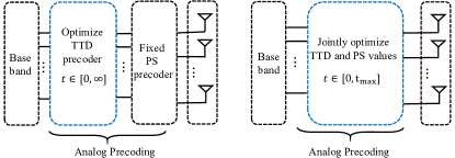
Figure 2: Comparison between beam squint compensation methods in the prior works [8, 9, 10] (left) and the proposed method in this work (right).

IV-A Problem Formulation

Ideally speaking, we wish to find $\{{\mathbf{t}}_{l}\}^{N_{RF}}_{l=1}$ and ${\mathbf{F}}_{1}$ satisfying ${\mathbf{F}}_{1}{\mathbf{F}}_{2,k}=\widetilde{{\mathbf{F}}}^{\star}_{k}$, $\forall k$. However, given fixed $l$, $m$, and $n$, solving $K$-coupled matrix equations is an ill-posed problem, because PSs only generate frequency-independent phase values. To overcome this, we approach to formulate a problem that optimizes ${\mathbf{F}}_{1}$ and $\{{\mathbf{t}}_{l}\}^{N_{RF}}_{l=1}$ by minimizing the difference between ${\mathbf{F}}_{1}{\mathbf{F}}_{2,k}$ and $\widetilde{{\mathbf{F}}}^{\star}_{k}$, $\forall k$:

$$\min_{{\mathbf{F}}_{1},\{{\mathbf{F}}_{2,k}\}_{k=1}^{K}}\!\!\!\!\!\!\!\!\!\! \frac{1}{K}\sum_{k=1}^{K}\left\|\widetilde{{\mathbf{F}}}^{\star}_{k}-{\mathbf{F}}_{1}{\mathbf{F}}_{2,k}\right\|^{2}_{F},$$ (20a)

subject to $$0\leq t^{(l)}_{m}\leq t_{\max},\forall l,m,$$ (20e)

$$|{\mathbf{F}}_{1}(i,j)|\in\!\left\{\frac{1}{\sqrt{N_{t}}},0\right\},\forall i,j,$$

$$|{\mathbf{F}}_{2,k}(p,q)|\in\!\{0,1\},\forall p,q,$$

$${\mathbf{F}}_{1}{\mathbf{F}}_{2,k}\in{\mathcal{F}}_{N_{t},N_{RF}},\forall k,$$

where the constraint (20e) indicates the restricted range of the time delay values per-TTD device, the constraint in (20e) is due to the definition of ${\mathbf{F}}_{1}$ in (7), the constraint in (20e) is due to the definition of ${\mathbf{F}}_{2,k}$ in (8), and the constraint in (20e) describes the constant modulus property of the analog precoder in (9). The constraints in (20e)-(20e) in conjunction with the coupling between ${\mathbf{F}}_{1}$ and ${\mathbf{F}}_{2,k}$ in (20a) make the problem difficult to solve. Besides, (20) can be viewed as a matrix factorization problem with non-convex constraints, which has been studied in the context of hybrid analog-digital precoding [15, 17, 34, 35, 36]. A common approach was applying block coordinate descent (BCD) and relaxing the constraints to deal with the non-convexity [15, 17, 34, 35, 36]. Unlike the prior approaches, we show that the original non-convex problem in (20) can be readily converted into an equivalent convex problem.

Based on the structure of ${\mathbf{F}}_{1}$ in (7) and the block diagonal structure of $\{{\mathbf{F}}_{2,k}\}_{k=1}^{K}$ in (8), the objective function in (20a) can be rewritten as

$$\!\!\!\!\frac{1}{K}\frac{1}{N_{t}}\sum_{k=1}^{K}\!\sum_{l=1}^{N_{RF}}\!\sum_{m=1}^{M}\!\sum_{n=1}^{N}\Big{|}e^{-j\pi\zeta_{k}\gamma^{(l)}_{n,m}}-e^{j\pi x^{(l)}_{n,m}}e^{-j\pi\zeta_{k}\vartheta^{(l)}_{m}}\Big{|}^{2}.$$ (21)

However, it is still difficult to deal with the objective function in (21) due to the unit modulus constraint. The following lemma shows that the optimization on the unit circle is equivalent to the optimization on the corresponding phase domain.

Lemma 1.

For $x\in{\mathbb{R}}$ and $y\in{\mathbb{R}}$, the following equality holds

$$\mathop{\mathrm{argmin}}\limits_{y\text{:}\mathop{\mathrm{mod}}(y,\pi)\neq x}|e^{jx}-e^{jy}|=\mathop{\mathrm{argmin}}\limits_{y\text{:}\mathop{\mathrm{mod}}(y,\pi)\neq x}|x-y|,$$ (22)

where $\mathop{\mathrm{mod}}(y,\pi)$ is $y$ modulo $\pi$.

Proof.

See Appendix B. ∎

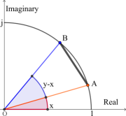
Figure 3: Conceptually illustration showing the relationship between the distance of two points on the unit modulus circle (the segment AB) and their relative phase difference (the arc corresponding to $y-x$)

Fig. 3 graphically visualizes the equivalence in Lemma 1. We let points A and B represent $e^{jx}$ and $e^{jy}$ in (22), respectively. It is not difficult to observe from Fig. 3 that minimizing the length of the segment AB with respect to B is equivalent to minimizing $|y-x|$ with respect to $y$, in which the latter is a convex optimization problem.

In what follows, Lemma 1 is exploited to convert the non-convex problem in (20) into a convex one. Incorporating Lemma 1 into (21) converts the problem in (20) to the following equivalent problem:

$$\!\!\!\!\!\!\!\!\!\!\min_{\{x^{(l)}_{n,m}\},\{\vartheta^{(l)}_{m}\}}\!\!\!\! \!\!\!\!\frac{1}{K}\!\sum\limits_{k=1}^{K}\!\!\sum\limits_{l=1}^{N_{RF}}\!\!\sum\limits_{m=1}^{M}\!\sum\limits_{n=1}^{N}\left|x^{(l)}_{n,m}\!\!-\!\zeta_{k}\vartheta^{(l)}_{m}\!\!+\!\zeta_{k}\gamma^{(l)}_{n,m}\right|^{2}\!\!\!\!,$$ (23a)

subject to $$\!\!\!\!0\leq\vartheta^{(l)}_{m}\leq\vartheta_{\max},~{}\forall l,m.$$ (23b)

Next, we turn (23) to a composite matrix optimization problem. The PS and TTD variables in (23) can be collected into a matrix ${\mathbf{A}}_{l}=[{\mathbf{a}}^{(l)}_{1}~{}\dots~{}{\mathbf{a}}^{(l)}_{M}]\in{\mathbb{R}}^{(N+1)\times M}$, where ${\mathbf{a}}^{(l)}_{m}=[({\mathbf{x}}^{(l)}_{m})^{T}~{}\vartheta^{(l)}_{m}]^{T}\in{\mathbb{R}}^{N+1}$. Containing the analog counterpart in $\widetilde{{\mathbf{F}}}^{\star}_{k}$ in a matrix ${\mathbf{B}}^{(l)}_{k}\in{\mathbb{R}}^{N\times M},$ where the $n$th row and $m$th column entry of ${\mathbf{B}}^{(l)}_{k}$ is $B^{(l)}_{k}(n,m)=-\zeta_{k}\gamma^{(l)}_{n,m}$, $\forall k,l,n,m$, the problem (23) becomes

$$\min_{\{{\mathbf{A}}_{l}\}^{N_{RF}}_{l=1}} \frac{1}{K}\sum\limits_{k=1}^{K}\sum\limits_{l=1}^{N_{RF}}\left\|{\mathbf{C}}_{k}{\mathbf{A}}_{l}-{\mathbf{B}}^{(l)}_{k}\right\|^{2}_{F},$$ (24a)

subject to $$\mathbf{0}^{T}_{M}\leq{\mathbf{e}}^{T}_{N+1}{\mathbf{A}}_{l}\leq\vartheta_{\max}\mathbf{1}^{T}_{M},~{}\forall l,$$ (24b)

where ${\mathbf{C}}_{k}=[{\mathbf{I}}_{N}~{}-\zeta_{k}\mathbf{1}_{N}]\in{\mathbb{R}}^{N\times(N+1)}$ and ${\mathbf{e}}_{N+1}\in{\mathbb{R}}^{N+1}$ is the $(N+1)$th column of the idendtity matrix ${\mathbf{I}}_{N+1}$. The vector inequalities in (24b) is the entry-wise inequalities.

By introducing ${\mathbf{C}}$ $=$ $\frac{1}{K}\sum_{k=1}^{K}{\mathbf{C}}^{T}_{k}{\mathbf{C}}_{k}$ $\in$ ${\mathbb{R}}^{(N+1)\times(N+1)}$, ${\mathbf{D}}_{l}$ $=$ $\frac{1}{K}\sum_{k=1}^{K}{\mathbf{C}}^{T}_{k}{\mathbf{B}}^{(l)}_{k}$ $\in$ ${\mathbb{R}}^{(N+1)\times M}$, and $c^{(l)}_{B}$ $=$ $\frac{1}{K}\sum_{k=1}^{K}\|{\mathbf{B}}^{(l)}_{k}\|^{2}_{F}$, the objective function in (24a) can be rewritten as $\frac{1}{K}\sum_{k=1}^{K}\sum_{l=1}^{N_{RF}}\Big{\|}{\mathbf{C}}_{k}{\mathbf{A}}_{l}-{\mathbf{B}}^{(l)}_{k}\Big{\|}^{2}_{F}$ $=$ $\sum_{l=1}^{N_{RF}}\sum_{m=1}^{M}\Big{(}\big{(}{\mathbf{a}}^{(l)}_{m}\big{)}^{T}{\mathbf{C}}{\mathbf{a}}^{(l)}_{m}-2\big{(}{\mathbf{d}}^{(l)}_{m}\big{)}^{T}{\mathbf{a}}^{(l)}_{m}\Big{)}+\sum_{l=1}^{N_{RF}}c^{(l)}_{B}$, where the ${\mathbf{d}}^{(l)}_{m}$ is the $m$th column of ${\mathbf{D}}_{l}$. Hence, the problem (24) is equivalently

$$\min_{{\mathbf{a}}^{(l)}_{m}}~{} ({\mathbf{a}}^{(l)}_{m})^{T}{\mathbf{C}}{\mathbf{a}}^{(l)}_{m}-2({\mathbf{d}}^{(l)}_{m})^{T}{\mathbf{a}}^{(l)}_{m},$$ (25a)

subject to $$0\leq{\mathbf{e}}_{N+1}^{T}{\mathbf{a}}^{(l)}_{m}\leq\vartheta_{\max},\forall l,m.$$ (25b)

The problem (25) can be viewed as a decomposition of (24) into $MN_{RF}$ independent problems. This decomposition reveals an alignment with the TTD and PS precoding architecture in Fig. 1c, where each RF feeds $M$ TTDs and each TTD feeds $N$ PSs. Thus, the problem in (25) is equivalent to optimizing the TTD and PS values of each RF chain branch independently.

IV-B Optimal Closed-form Solution

In this subsection, we find the optimal closed-form solution of the convex problem (25). We start by deriving the expression of ${\mathbf{C}}$ in (25a). To this end, we first define the constant $\Gamma=N+\eta$, where $\eta=\frac{NB^{2}}{f^{2}_{c}}\frac{(K^{2}-1)}{12K^{2}}$. For ${\mathbf{C}}_{k}$ in (24), we have ${\mathbf{C}}^{T}_{k}{\mathbf{C}}_{k}=\begin{bmatrix}{\mathbf{I}}_{N}&-\zeta_{k}\mathbf{1}_{N}\\ -\zeta_{k}\mathbf{1}^{T}_{N}&N\zeta^{2}_{k}\end{bmatrix}$, where $\zeta_{k}$ is defined in (4). After some algebraic manipulations, it is readily verified that

$$\sum_{k=1}^{K}\zeta_{k}\!\!\!\! = \!\!\!\!K,$$ (26a)

$$\sum_{k=1}^{K}\zeta^{2}_{k}\!\!\!\! = \!\!\!\!K\Big{(}1+\frac{\eta}{N}\Big{)}.$$ (26b)

Then, $~{}~{}{\mathbf{C}}~{}~{}=~{}~{}~{}~{}\frac{1}{K}\sum_{k=1}^{K}{\mathbf{C}}^{T}_{k}{\mathbf{C}}_{k}$ is simplified, based on (26), to ${\mathbf{C}}\!=\!\begin{bmatrix}\!{\mathbf{I}}_{N}\!&\!-\mathbf{1}_{N}\\ -\mathbf{1}^{T}_{N}\!&\!\Gamma\!\!\!\end{bmatrix}$. The inverse of ${\mathbf{C}}$ is given by

$${\mathbf{C}}^{-1}=\begin{bmatrix}({\mathbf{I}}_{N}+\frac{1}{\eta}\mathbf{1}_{N}\mathbf{1}^{T}_{N})&\frac{1}{\eta}\mathbf{1}_{N}\\ \frac{1}{\eta}\mathbf{1}^{T}_{N}&\frac{1}{\eta}\end{bmatrix},$$ (27)

which allows us to obtain

$${\mathbf{e}}^{T}_{N+1}{\mathbf{C}}^{-1}{\mathbf{e}}_{N+1}=\frac{1}{\eta}.$$ (28)

Defining ${\mathbf{b}}^{(l)}_{k,m}\!=\![-\zeta_{k}\gamma^{(l)}_{1,m}~{}\dots~{}-\zeta_{k}\gamma^{(l)}_{N,m}]^{T}$ as the $m$th column of ${\mathbf{B}}^{(l)}_{k}$ in (24), it is straightforward that

$${\mathbf{d}}^{(l)}_{m}=\begin{bmatrix}\frac{1}{K}\sum_{k=1}^{K}{\mathbf{b}}^{(l)}_{k,m}\\ \frac{1}{K}\sum_{k=1}^{K}-\zeta_{k}\mathbf{1}^{T}_{N}{\mathbf{b}}^{(l)}_{k,m}\end{bmatrix}\in{\mathbb{R}}^{(N+1)\times 1}.$$ (29)

From (27) and (29), it is readily verified that

$$\!\!\!\!\!\!\!\!{\mathbf{e}}_{N+1}^{T}{\mathbf{C}}^{-1}{\mathbf{d}}^{(l)}_{m}\!\!\!\! = \!\!\!\!\frac{1}{\eta}\frac{1}{K}\sum_{k=1}^{K}\Big{(}(1-\zeta_{k})\sum_{n=1}^{N}{\mathbf{b}}^{(l)}_{k,m}(n,1)\Big{)},$$ (30a)

$$= \frac{(2m-1)N-1}{2}\psi_{l},$$ (30b)

where the ${\mathbf{b}}^{(l)}_{k,m}(n,1)$ in (30a) is the $n$th entry of ${\mathbf{b}}^{(l)}_{k,m}$, $n=1,2,\dots,N$ and (30b) follows from the facts that ${\mathbf{b}}^{(l)}_{k,m}(n,1)$ $=$ $-\zeta_{k}\gamma^{(l)}_{n,m}$ and $\gamma^{(l)}_{n,m}$ $=$ $((m-1)N+n-1)\psi_{l}$.

Based on the results in (28) and (30b), the optimal closed-form solution of the problem in (25) is summarized below.

Theorem 1.

The optimal solution ${{\mathbf{a}}^{(l)}_{m}}^{\star}=[({{\mathbf{x}}^{(l)}_{m}}^{\star})^{T},{\vartheta^{(l)}_{m}}^{\star}]^{T}$ to (25) is given by

$$\!\!\!\!\!\!\!\!\!\!\!\!\!\!\!\!{x^{(l)}_{n,m}}^{\footnotesize\star}= \!\!\frac{N-2n+1}{2}\psi_{l}, 0\leq\psi_{l}\leq\frac{4f_{c}t_{\max}}{(2m-1)N-1}$$ ​​​​​​​​ if ,​​​​​​​​ (31a)

$$\!\!\!\!\!\!\!\!\!\!\!\!\!\!\!\!{x^{(l)}_{n,m}}^{\footnotesize\star}= \vartheta_{\max}-\gamma^{(l)}_{n,m},$$ ​​​​​​​​ otherwise, (31b)

for $l=1,2,\dots,N_{RF}$, $n=1,2,\dots,N$, $m=1,2,\dots,M$, and ${\vartheta^{(l)}_{m}}^{\star}=2f_{c}{t^{(l)}_{m}}^{\star}$, where the ${t^{(l)}_{m}}^{\star}$ is

$${t^{(l)}_{m}}^{\star}= \frac{(2m-1)N-1}{4f_{c}}\psi_{l},\!\!\!\! 0\leq\psi_{l}\leq\frac{4f_{c}t_{\max}}{(2m-1)N-1}$$ if ,​​ (32a)

$${t^{(l)}_{m}}^{\star}= t_{\max},\!\!\!\!$$ otherwise, ​​ (32b)

for $l=1,2,\dots,N_{RF}$ and $m=1,2,\dots,M$.

Proof.

See Appendix C. ∎

Remark 2.

The solutions in (32b) and (31b) differentiate them from prior approaches to solving related problems. For instance, the PS values in [32] were not optimized and given by $x^{(l)}_{n,m}=-(n-1)\psi_{l}$, $\forall n$. The time delay value of the $m$th TTD was $t^{(l)}_{m}=m\frac{N\psi_{l}}{2f_{c}}$ in [32]; as $m$ increases, the $t^{(l)}_{m}$ could be larger than $t_{\max}$, in which case such $t^{(l)}_{m}$ needs to be floored to the $t_{\max}$, resulting in performance deterioration. As will be discussed in Section V, however, when all TTD values are smaller than $t_{\max}$, the approaches in [32, 9] achieve the same array gain performance as the proposed approach, meaning that the designs in [32, 9] is a special case of Theorem 1.

In the following, the benefits of the proposed joint TTD and PS precoder optimization method are discussed. The optimal condition in (31a) and (32a) can be rewritten as

$$\frac{(2m-1)N-1}{4f_{c}}\psi_{l}\leq t_{\max}.$$ (33)

When (33) is satisfied, the beam squint is compensated effectively. However, the condition (33) may be violated, for example, when either $t_{\max}$ becomes small or $N$ becomes large (i.e., $N_{t}$ tends to be large while fixing $M$, i.e., $N=\frac{N_{t}}{M}$). Based on the condition in (33), we obtain selection criteria (rule of thumb) on the required number of transmit antennas $(N_{t})$ and the value of maximum time delay $(t_{\max})$ for the best beam squint compensation as follows.

IV-B1 $N_{t}$ Selection Criterion

Given the number of TTDs per RF chain $M$ and the $t_{\max}$ values determined by the employed TTD devices, choose $N_{t}$ such that

$$N_{t}\leq\frac{M}{2m-1}+\frac{4M}{(2m-1)}\frac{1}{\psi_{l}}f_{c}t_{\max},\forall l,m,$$ (34)

where (34) is a result of substituting $N=\frac{N_{t}}{M}$ into (33). The inequality in (34) can be rewritten as

$$N_{t} \leq \min_{l,m}\Big{(}\frac{M}{2m-1}+\frac{4M}{(2m-1)}\frac{1}{\psi_{l}}f_{c}t_{\max}\Big{)},$$ (35a)

$$= \frac{M}{2M-1}+\frac{4M}{(2M-1)}\frac{1}{\max_{l}\psi_{l}}f_{c}t_{\max}.$$ (35b)

The $\min_{l,m}$ in (35a) is taken so that (34) holds for all $MN_{RF}$ TTDs. The (35b) follows from substituting $m=M$ and $\psi_{l}$ by its maximum value $\max_{l}\psi_{l}$ into (35a).

IV-B2 $t_{\max}$ Selection Criterion

Equivalently, given the number of TTDs per RF chain $M$ and the number of transmit antennas $N_{t}$, the TTD value should be chosen to satisfy

$$t_{\max}\geq\psi_{l}\frac{(2m-1)N_{t}-M}{4M}\frac{1}{f_{c}},\forall l,m.$$ (36)

The inequality in (36) can be rewritten as

$$t_{\max} \geq \max_{l,m}\Big{(}\psi_{l}\frac{(2m-1)N_{t}-M}{4M}\frac{1}{f_{c}}\Big{)},$$ (37a)

$$= (\max_{l}\psi_{l})\frac{(2M-1)N_{t}-M}{4M}\frac{1}{f_{c}}.$$

The system parameter selection criteria in (35b) and (37a) give an idea of the values of $N_{t}$ and $t_{\max}$ for the best beam squint compensation given a fixed number of TTDs per RF chain $M$. In practice, it is critical to install an appropriate number of TTDs per RF chain $M$ to reduce the power consumption of the analog precoder because there are total $N_{RF}M$ TTDs and $N_{RF}N_{t}$ PSs in the analog precoder as shown in Fig. 1c.

IV-C The Number of TTDs per RF Chain

In this subsection, we further exploit the closed-form solution of the TTD and PS precoders in Theorem 1 to characterize the minimum number of TTDs per RF chain $M$ given a predefined array gain performance while assuming that the constraint in (37a) is always satisfied and the number of transmit antennas $N_{t}$ is fixed. To this end, we formulate a problem that minimizes $M$ to guarantee a given array gain performance:

$$\min_{M} M,$$ (38a)

subject to $$N_{t}=MN,~{}g({\mathbf{f}}^{(l)}_{k},\psi_{k,l})\geq g_{0},\forall k,l,$$ (38b)

where the second constraint in (38b) describes the array gain guarantee with the threshold $0<g_{0}<1$. We note that the total power consumption of the analog precoder can be modeled as $P_{total}=N_{RF}MP_{TTD}+N_{RF}N_{t}P_{TTD}$, where $P_{TTD}$ and $P_{PS}$ are the power consumption of a TTD and a PS, respectively. Hence, given the fixed values of $N_{t}$, $P_{TTD}$, and $P_{PS}$, the objective of minimizing the power consumption (i.e., $\min_{M}P_{total}$) is equivalent to the objective in (38).

In solving (38), we first compute the array gain $g({\mathbf{f}}^{(l)}_{k},\psi_{k,l})$ defined in (12) with the optimal PS values in (31a) and the optimal TTD values in (32a), i.e., $g({\mathbf{f}}^{(l)}_{k},\psi_{k,l})$ $=$ $\frac{1}{N_{t}}\Big{|}\!\sum\limits_{m=1}^{M}\!\sum\limits_{n=1}^{N}\!e^{j\pi\zeta_{k}\gamma^{(l)}_{n,m}}e^{j\pi\frac{N-2n+1}{2}\psi_{l}}e^{-j\pi\zeta_{k}\frac{(2m-1)N-1}{2}\psi_{l}}\!\Big{|}$, yielding

$$g({\mathbf{f}}^{(l)}_{k},\psi_{k,l})=\left|\frac{\sin(N\Delta_{k,l})}{N\sin(\Delta_{k,l})}\right|.$$ (39)

Incorporating (39) into the second constraint in (38b) and substituting $\frac{N_{t}}{M}$ for $N$, the problem is converted to:

$$\min_{M} M,$$ (40a)

subject to $$\bigg{|}\frac{\sin\left(\frac{N_{t}}{M}\Delta_{k,l}\right)}{\frac{N_{t}}{M}\sin(\Delta_{k,l})}\bigg{|}\geq g_{0},\forall k,l.$$ (40b)

The problem in (40) can be viewed as finding the minimum element in the feasible set ${\mathcal{M}}=\left(\bigcap_{k=1,l=1}^{K,L}{\mathcal{M}}_{k,l}\right)\cap{\mathcal{N}}_{t}$, where ${\mathcal{M}}_{k,l}=\bigg{\{}M\in{\mathbb{R}}\colon\Big{|}\frac{\sin(\frac{N_{t}}{M}\Delta_{k,l})}{\frac{N_{t}}{M}\sin(\Delta_{k,l})}\Big{|}\geq g_{0}\bigg{\}}$, for $k=1,2,\dots,K$ and $l=1,2,\dots,L$, and ${\mathcal{N}}_{t}=\left\{m\in{\mathbb{N}}\colon m|N_{t}\right\}$, where $m|N_{t}$ means that $m$ is a divisor of $N_{t}$. Thus, solving the problem (40) using the greedy search method requires the construction of $KL+1$ sets $\{{\mathcal{M}}_{k,l}\}$ and ${\mathcal{N}}_{t}$, which is demanding when the number of OFDM subcarriers is large in the wideband THz massive MIMO systems.

To cope with these difficulties, we propose to approximate the constraint in ${\mathcal{M}}_{k,l}$, i.e., the constraint in (40b) as

$$|q(\Delta_{k,l})|\geq g_{0},\forall k,l,$$ (41)

where $q(x)=1+\frac{1}{6}\left(1-\frac{N^{2}_{t}}{M^{2}}\right)x^{2}$ and it is obtained by the Taylor expansion $\frac{\sin\left(\frac{N_{t}}{M}x\right)}{\frac{N_{t}}{M}\sin(x)}=q(x)+{\mathcal{O}}(x^{4})$ derived at $x=0$. Incorporating (41) into (40) and noting that $|x|\geq x$, the problem in (40) is relaxed to

$$\min_{M} M,$$ (42a)

subject to $$M\in{\mathcal{N}}_{t},~{}q(\Delta_{k,l})\geq g_{0},\forall k,l.$$ (42b)

About the optimal solution of (42), denoted as $M^{\star}$, we have the following theorem.

Theorem 2.

Given the fixed $N_{t}$, $B$, $f_{c}$, and $K$, the ${M}^{\star}$ of (42) is

$${M}^{\star}=\left\lceil~{}\sqrt{\frac{N^{2}_{t}}{1+\Omega(g_{0},B)}}~{}\right\rceil_{N_{t}},$$ (43)

where $\Omega(g_{0},B)=\frac{6(1-g_{0})}{\left(\frac{\pi}{2}\frac{B}{f_{c}}\frac{K-1}{2K}\right)^{2}\max_{l}\psi^{2}_{l}}$ and $\lceil x\rceil_{N_{t}}$ denotes the smallest integer greater than or equal to $x$ that is a divisor of $N_{t}$.

Proof.

See Appendix D. ∎

Remark 3.

To understand the relationship between the $M^{\star}$ in (43) and the system parameters, we first relax its integer constraint, which leads to $M^{\star}=\sqrt{\frac{N^{2}_{t}}{1+\Omega(g_{0},B)}}$. In the regime of a large number of OFDM subcarriers ($K\gg 1$), we have $\frac{K-1}{2K}\approx\frac{1}{2}$, leading to $M^{\star}\approx\sqrt{\frac{N^{2}_{t}(\frac{\pi}{4}\frac{B}{f_{c}})^{2}\max_{l}\psi^{2}_{l}}{6(1-g_{0})}}=\left(\frac{\pi N_{t}}{4f_{c}}\sqrt{\frac{\max_{l}\psi^{2}_{l}}{6(1-g_{0})}}\right)B$. Given a fixed $N_{t}$, it reveals that the minimum required number of TTDs that ensures a predefined array gain performance grows linearly with the bandwidth $B$.

V Simulation Results

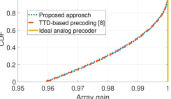
(a)

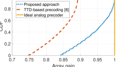
(b)

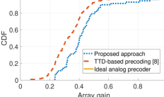
(c)

Figure 4: ​CDF of the array gain with different number of transmit antennas ($N_{t}$) values:​ (a) $N_{t}\!=\!128$, (b) $N_{t}\!=\!256$, and c) $N_{t}\!=\!512$.

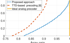
(a)

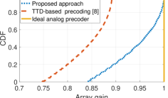
(b)

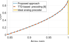
(c)

Figure 5: ​CDF of array gain with different maximum time delay ($t_{\max}$) values: (a) $t_{\max}\!=\!320$ ps, (b) $t_{\max}\!=\!340$ ps, and (c) $t_{\max}\!=\!400$ ps.

In this section, we demonstrate the benefits of the proposed joint TTD and PS precoding by comparing it with the (i) state-of-the-art approach proposed in [8] and (ii) ideal analog precoding $\{\widetilde{{\mathbf{F}}}^{\star}_{k}\}^{K}_{k=1}$ in (14) in terms of array gain and achievable rate performance. Throughout the simulation, the system parameters are set as follows unless otherwise stated: the central carrier frequency $f_{c}\!=\!300$ GHz, bandwidth $B\!=\!30$ GHz, the number of OFDM subcarriers $K\!=\!129$, number of transmit antennas $N_{t}\!=\!256$, number of receive antennas $N_{r}\!=\!4$, number of RF chain $N_{RF}\!=\!4$, number of data stream $N_{s}\!=\!4$, and SNR $\rho\!=\!3$ dB. The number of TTDs per RF chain $M\!=\!16$, the number of PSs per TTD $N\!=\!16$, and the maximum time delay $t_{\max}\!=\!340$ ps. The AoDs and AoAs are uniformly drawn in $[\frac{-\pi}{2},\frac{\pi}{2}]$.

V-A Beam Squint Compensation

To demonstrate the array gain performance, we measure the empirical cumulative distribution function (CDF) of the array gain $G_{\psi}(x)$ at the central spatial direction $\psi$, where $G_{\psi}(x)=\frac{1}{K}\sum_{k=1}^{K}\mathds{1}_{g}(k,x)$, $x$ represents the array gain $0\leq x\leq 1$ in (5), and the indicator function $\mathds{1}_{g}(k,x)$ takes values

$$\mathds{1}_{g}(k,x)=\left\{\begin{array}[]{ll}1,&\text{if }g({\mathbf{f}}^{(l)}_{k},\psi_{k})\leq x,\\ 0,&\text{otherwise},\end{array}\right.$$

where $g({\mathbf{f}}^{(l)}_{k},\psi_{k})$ is computed as in (5) with the spatial direction $\psi=0.8$.

Fig. 4 displays the empirical CDF curves of the array gain when the number of transmit antennas $N_{t}$ takes the values from $\{128,256,512\}$. When $N_{t}=128$ the proposed approach and benchmark [8] have the same array gain performance because the designed TTD values in both approaches are smaller than the preset $t_{\max}=340$ ps. When $N_{t}=256$ (Fig. 4b) and $N_{t}=512$ (Fig. 4c), the proposed approach and benchmark [8] suffer from the array gain loss because the degree of beam squint increases as $N_{t}$ grows (i.e., Proposition 1). Nevertheless, the proposed approach provides an enhanced beam squint compensation capability compared to the benchmark. This is due to the fact that as $N_{t}$ grows some of the time delay values of the benchmark [8] become larger than $t_{\max}=340$ ps in which case the time delay value needs to be floored to the $t_{\max}$. It can be observed in Fig. 4b that around $80\%$ of OFDM subcarriers achieve the array gain $\geq 0.9$ for the proposed approach. For the benchmark [8], on the other hand, there is no OFDM subcarriers that reach $0.9$ array gain performance.

Fig. 5 shows the empirical CDF curves of the array gain when the maximum time delay value $t_{\max}$ takes values in $\{320,340,400\}$ ps while fixing $N_{t}=256$. Seen from Fig. 5, the proposed approach shows the consistent array gain in all cases while the curve of the benchmark [8] converges to the proposed approach when $t_{\max}=400$ ps as shown in Fig. 5c. When $t_{\max}=320$ ps (Fig. 5a) and $t_{\max}=340$ ps (Fig. 5b), the proposed approach outperforms the benchmark. It is noteworthy to point out that there is no OFDM subcarriers that reach array gain $\geq 0.93$ of the benchmark when $t_{\max}\leq 340$ ps.

Overall, the trends in Figs. 4-5 reaffirm Remark 2 indicating that the benchmark is a special cases of the proposed joint optimization. Figs. 4-5 also verify the efficacy of the proposed approach when the $N_{t}$ and $t_{\max}$ are chosen to meet the criterion in (35b) and (37a) such that $N_{t}\leq 256$ and $t_{\max}\geq 320$ ps.

V-B Achievable Rate Performance

In this subsection, we demonstrate the empirical CDF of the achievable rate per subcarrier $\widetilde{R}(x)$, which is defined as $\widetilde{R}(x)$ $=$ $\frac{1}{K}\sum_{k=1}^{K}\mathds{1}_{r}(k,x)$ for $x\geq 0$, where the indicator function $\mathds{1}_{r}(k,x)$ is given by

$$\mathds{1}_{r}(k,x)=\left\{\begin{array}[]{ll}1,&\text{ if }R_{k}\leq x,\\ 0,&\text{otherwise},\end{array}\right.$$

where the $R_{k}$ is defined by $R_{k}=\log_{2}\mathop{\mathrm{det}}({\mathbf{I}}_{N_{s}}+\frac{\rho}{N_{s}}{\mathbf{H}}_{k}{\mathbf{F}}_{k}{\mathbf{W}}_{k}{\mathbf{W}}^{H}_{k}{\mathbf{F}}^{H}_{k}{\mathbf{H}}^{H}_{k})$. The digital precoders $\{{\mathbf{W}}_{k}\}_{k=1}^{K}$ are designed by choosing $N_{s}$ dominant eigenvectors of $\widetilde{{\mathbf{H}}}^{H}_{k}\widetilde{{\mathbf{H}}}_{k}$, where $\widetilde{{\mathbf{H}}}_{k}={\mathbf{H}}_{k}{\mathbf{F}}_{k}$, $\forall k$. Herein, we adopt the same channel model as in [8], where the path delay is uniformly distributed from $0$ to $20$ ms and the channel path gain is i.i.d following the complex Gaussian distribution with zero mean and variance 1.

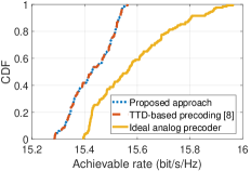
(a)

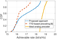
(b)

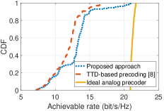
(c)

Figure 6: CDF of achievable rate per subcarrier with different number of transmit antennas ($N_{t}$) values: (a) $N_{t}\!=\!128$, (b) ​$N_{t}\!=\!256$, and (c)​ $N_{t}\!=\!512$.

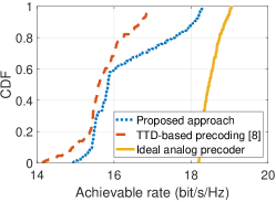
(a)

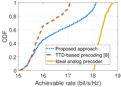
(b)

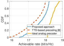
(c)

Figure 7: CDF of achievable rate per subcarrier with different $t_{\max}$ values: (a) $t_{\max}=320$ ps, (b) $t_{\max}=340$ ps, and (c) $t_{\max}=400$ ps.

Fig. 6 presents the empirical CDF curves of the achievable rate when $N_{t}$ takes values in $\{128,256,512\}$. When $N_{t}=128$ in Fig. 6a, the proposed method and the benchmark [8] show the same achievable rate performance because, as discussed in Remark 2, when $N_{t}$ is relatively small all TTD values are smaller than $t_{\max}$ and the proposed method and the benchmark become equivalent. As seen in Fig. 6b ($N_{t}=256$) and Fig. 6c ($N_{t}=512$), on the other hand, the proposed approach shows an improved achievable rate performance compared to the benchmark, which is aligned with the array gain performance trends in Figs. 4b-4c, respectively. The curve of the proposed approach is closer to the ideal achievable rate curve. For instance in Fig. 6b, around $40\%$ of OFDM subcarrier of the proposed approach has the achievable rate $\geq 17$ (bits/s/Hz) while the majority of the OFDM subcarriers of the benchmark have the achievable rate $<17$ (bits/s/Hz).

Fig. 7 demonstrates the empirical CDF curves of the achievable rate when $t_{\max}$ increases from $t_{\max}=320$ ps to $t_{\max}=400$ ps. It can be observed from Fig. 7 that the proposed approach outperforms the benchmark as $t_{\max}$ increases. In Figs. 7a-7b, the proposed method always presents a better achievable rate performance than the benchmark. These align with array gain performance curves in Figs. 5a-5b, respectively.

Figs. 6-7 verify the benefits of the joint TTD and PS optimization of the proposed approach on the achievable rate performance. Similar to Figs. 4-5, Figs. 6-7 demonstrate the efficacy of the proposed joint optimization when $N_{t}$ and $t_{\max}$ are chosen to meet the criterion in (35b) and (37a) such that $N_{t}\leq 256$ and $t_{\max}\geq 320$ ps.

V-C Array Gain Performance Guarantee of $\widetilde{M}^{\star}$ in (43)

In this subsection, we demonstrate the array gain performance guarantee provided by the minimum required number of TTDs per RF chain $\widetilde{M}^{\star}$ in (43) of Theorem 2. Similar to Section V-A, we evaluate the empirical CDF of the array gain $G_{\psi}(x)$ at the spatial direction $\psi=0.8$ except for that we assume $N_{t}=720$ and $t_{\max}=1000$ ps in this simulation. The array gain threshold is set to $g_{0}=0.9$ in (43). Incorporating $g_{0}$ and the system parameters into (43) yields $\widetilde{M}^{\star}=\left\lceil\sqrt{\frac{720^{2}}{\Omega(0.9,30)}}\right\rceil_{720}=60$.

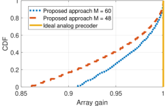
Figure 8: CDF of array gain of the proposed approach with different number of TTDs per RF chain ($M$) values.

Fig. 8 illustrates the CDF of the array gain when $M=\widetilde{M}^{\star}=60$ and $M=48$, where $M=48$ is chosen to be the largest divisor of $N_{t}$ that is smaller than $\widetilde{M}^{\star}=60$. We note that the condition in (37a) is satisfied for both values of $M$ when $t_{\max}=1000$ ps. As shown in Fig. 8, for the optimized $\widetilde{M}^{\star}=60$, every OFDM subcarrier satisfies the array gain $\geq 0.9$. However, when $M=48$, there are $18\%$ of the OFDM subcarriers that have the array gain $<0.9$. Hence, the curves in Fig. 8 verified that the $\widetilde{M}^{\star}=60$ is the minimum number of TTDs per RF chain to provide the minimum array gain $g_{0}=0.9$.

VI Conclusion

In this paper, we presented a new approach to the problem of compensating the beam squint effect arising in wideband THz hybrid massive MIMO systems. We showed that the ideal analog precoder that completely compensates for the beam squint is the one that maximizes the achievable rate lower bound. A novel TTD-based hybrid precoding approach was proposed by jointly optimizing the TTD and PS precoders under the per-TTD time delay constraints. The joint optimization problem was formulated in the context of minimizing the distance between the ideal analog precoder and the product of the PS and TTD precoders. By transforming the original problem into the phase domain, the original problem was converted to an equivalent convex problem, which allowed us to find a closed form of the global optimal solution. On the basis of the closed-form expression of our solution, we presented the selection criteria for the required number of transmit antennas and the value of maximum time delay. Taking advantage of the proposed joint TTD and PS precoder optimization approach, we quantified the minimum number of TTDs required to provide an array gain performance guarantee, while minimizing the analog precoder power consumption. Through simulations, we affirmed the superiority of our joint TTD and PS optimization with the array gain performance guarantee.

Appendix A Proof of Proposition 2

We note that showing Proposition 2 is equivalent to prove

$$\widetilde{{\mathbf{F}}}^{\star}_{k}\!\!\!\! = \mathop{\mathrm{argmax}}_{{\mathbf{F}}_{k}}\hskip 14.22636pt\lim_{N_{t}\rightarrow\infty}\log_{2}(\Xi_{k}),$$ (44b)

$$\text{subject to}\ \ \ \ \ {\mathbf{F}}_{k}\in{\mathcal{F}}_{N_{t},N_{RF}},$$

for $k=1,\dots,K$. The objective in (44b) is decomposed into

$$\!\!\!\!\!\!\!\!\log_{2}\mathop{\mathrm{det}}\left(\Sigma^{2}_{k}{\mathbf{P}}^{H}_{k}\widetilde{{\mathbf{F}}}^{\star H}_{k}{\mathbf{F}}_{k}{\mathbf{W}}_{k}{\mathbf{W}}^{H}_{k}{\mathbf{F}}^{H}_{k}\widetilde{{\mathbf{F}}}^{\star}{\mathbf{P}}_{k}\right)\\ \!\!\!\!=\log_{2}\mathop{\mathrm{det}}\left(\Sigma^{2}_{k}{\mathbf{P}}^{H}_{k}{\mathbf{W}}_{k}{\mathbf{W}}^{H}_{k}{\mathbf{P}}_{k}\right)\!+\!\log_{2}\mathop{\mathrm{det}}\left({\mathbf{F}}^{H}_{k}\widetilde{{\mathbf{F}}}^{\star}_{k}\widetilde{{\mathbf{F}}}^{\star H}_{k}{\mathbf{F}}_{k}\right).\!\!\!\!$$ (45)

Applying the Hadamard’s inequality to ${\mathbf{F}}^{H}_{k}\widetilde{{\mathbf{F}}}^{\star}_{k}\widetilde{{\mathbf{F}}}^{\star H}_{k}{\mathbf{F}}_{k}$ yields

$$\!\!\mathop{\mathrm{det}}\left({\mathbf{F}}^{H}_{k}\widetilde{{\mathbf{F}}}^{\star}_{k}\widetilde{{\mathbf{F}}}^{\star H}_{k}{\mathbf{F}}_{k}\right)\!\leq\!\!\prod_{l=1}^{N_{RF}}\!\!\left({\mathbf{f}}^{(l)}_{k}\right)^{H}\widetilde{{\mathbf{F}}}^{\star}_{k}\widetilde{{\mathbf{F}}}^{\star H}_{k}{\mathbf{f}}^{(l)}_{k}=\prod_{l=1}^{N_{RF}}\left\|\widetilde{{\mathbf{F}}}^{\star H}_{k}{\mathbf{f}}^{(l)}_{k}\right\|^{2}_{2}\!\!.$$ (46)

The ${\mathbf{f}}^{(l)}_{k}$ in (46) is the $l$th column of ${\mathbf{F}}_{k}$ and $\|{\mathbf{f}}^{(l)}_{k}\|^{2}_{2}$ $=$ $1$ because of the constant modulus property in (44b). Thus, the following holds

$$\left\|\widetilde{{\mathbf{F}}}^{\star H}_{k}{\mathbf{f}}^{(l)}_{k}\right\|^{2}_{2}~{}\leq~{}\Lambda_{\max}(\widetilde{{\mathbf{F}}}^{\star H}_{k}\widetilde{{\mathbf{F}}}^{\star}_{k})\stackrel{{\scriptstyle\boldsymbol{\cdot}}}{{=}}1,$$ (47)

where $\Lambda_{\max}(\widetilde{{\mathbf{F}}}^{\star H}_{k}\widetilde{{\mathbf{F}}}^{\star}_{k})$ is the maximum eigenvalue of $\widetilde{{\mathbf{F}}}^{\star H}_{k}\widetilde{{\mathbf{F}}}^{\star}_{k}$ and the last equality is due to the fact that $\widetilde{{\mathbf{F}}}^{\star H}_{k}\widetilde{{\mathbf{F}}}^{\star}_{k}\stackrel{{\scriptstyle\boldsymbol{\cdot}}}{{=}}{\mathbf{I}}_{N_{RF}}$. Incorporating (47) into (46) gives $\mathop{\mathrm{det}}\left({\mathbf{F}}^{H}_{k}\widetilde{{\mathbf{F}}}^{\star}_{k}\widetilde{{\mathbf{F}}}^{\star H}_{k}{\mathbf{F}}_{k}\right)\stackrel{{\scriptstyle\boldsymbol{\cdot}}}{{\leq}}1$. Therefore, applying (45) leads to $\log_{2}\mathop{\mathrm{det}}\left(\Sigma^{2}_{k}{\mathbf{P}}^{H}_{k}\widetilde{{\mathbf{F}}}^{\star H}_{k}{\mathbf{F}}_{k}{\mathbf{W}}_{k}{\mathbf{W}}^{H}_{k}{\mathbf{F}}^{H}_{k}\widetilde{{\mathbf{F}}}^{\star}{\mathbf{P}}_{k}\right)$ $\stackrel{{\scriptstyle\boldsymbol{\cdot}}}{{\leq}}$ $\log_{2}\mathop{\mathrm{det}}\left(\Sigma^{2}_{k}{\mathbf{P}}^{H}_{k}{\mathbf{W}}_{k}{\mathbf{W}}^{H}_{k}{\mathbf{P}}_{k}\right)$, where the equality holds if and only if ${\mathbf{F}}_{k}=\widetilde{{\mathbf{F}}}^{\star}_{k}$. This completes the proof.

Appendix B Proof of lemma 1

Without loss of generality, we assume $0\!<\!|x\!-\!y|\!<\!\pi$. Then, ${\mathop{\mathrm{argmin}}}_{0<|x-y|<\pi}{|e^{jx}-e^{jy}|}={\mathop{\mathrm{argmin}}}_{0<|x-y|<\pi}\Big{|}\sin\Big{(}\frac{x-y}{2}\Big{)}\Big{|}$ $=$ ${\mathop{\mathrm{argmin}}}_{0<|x-y|<\pi}\sin\Big{(}\Big{|}\frac{x-y}{2}\Big{|}\Big{)}=\mathop{\mathrm{argmin}}_{0<|x-y|<\pi}|x-y|$, where the last step follows from the fact that $\sin(z)$ is an increasing function of $0<z<\frac{\pi}{2}$. This completes the proof.

Appendix C Proof of theorem 1

To prove Theorem 1, we start by formulating the Lagrangian of (25), which is given by

$${\mathcal{L}}({\mathbf{a}}^{(l)}_{m},\lambda_{1},\lambda_{2})={\mathbf{a}}^{(l)T}_{m}{\mathbf{C}}{\mathbf{a}}^{(l)}_{m}-2{\mathbf{d}}^{(l)T}_{m}{\mathbf{a}}^{(l)}_{m}+\\ \lambda_{1}({\mathbf{e}}_{N+1}^{T}{\mathbf{a}}^{(l)}_{m}-\vartheta_{\max})+\lambda_{2}(-{\mathbf{e}}_{N+1}^{T}{\mathbf{a}}^{(l)}_{m}),$$ (48)

where $\lambda_{1}\geq 0$ and $\lambda_{2}\geq 0$ are the Largrangian multipliers. After incorporating the first order necessary condition for ${\mathbf{a}}_{m}^{(l)}$ in (48), the Karush–Kuhn–Tucker (KKT) conditions of (25) are given by:

$$\left\{\begin{array}[]{ll}2{\mathbf{C}}{\mathbf{a}}^{(l)}_{m}-2{\mathbf{d}}^{(l)}_{m}+\lambda_{1}{\mathbf{e}}_{N+1}-\lambda_{2}{\mathbf{e}}_{N+1}&=0,\\ \lambda_{1}({\mathbf{e}}_{N+1}^{T}{\mathbf{a}}^{(l)}_{m}-\vartheta_{\max})&=0,\\ \lambda_{2}(-{\mathbf{e}}_{N+1}^{T}{\mathbf{a}}^{(l)}_{m})&=0,\\ \lambda_{1}\geq 0,\lambda_{2}\geq 0.\end{array}\right.$$ (49)

It is easy to observe that when $\lambda_{1}>0$ and $\lambda_{2}>0$, there is no solution for (49) because solving (49) leads to ${\mathbf{e}}_{N+1}^{T}{\mathbf{a}}^{(l)}_{m}=\vartheta_{\max}>0$ and $-{\mathbf{e}}_{N+1}^{T}{\mathbf{a}}^{(l)}_{m}=0$, which is a contradiction. When $\lambda_{1}=\lambda_{2}=0$, (49) yields ${\mathbf{a}}^{(l)}_{m}={\mathbf{C}}^{-1}{\mathbf{d}}^{(l)}_{m}$ for $0\leq{\mathbf{e}}_{N+1}^{T}{\mathbf{C}}^{-1}{\mathbf{d}}^{(l)}_{m}\leq\vartheta_{\max}$ because $0\leq{\mathbf{e}}_{N+1}^{T}{\mathbf{a}}^{(l)}_{m}\leq\vartheta_{\max}$. When $\lambda_{1}>0$ and $\lambda_{2}=0$, (49) gives ${\mathbf{a}}^{(l)}_{m}={\mathbf{C}}^{-1}({\mathbf{d}}^{(l)}_{m}-\frac{1}{2}\lambda_{1}{\mathbf{e}}_{N+1})$ for ${\mathbf{e}}_{N+1}^{T}{\mathbf{C}}^{-1}{\mathbf{d}}^{(l)}_{m}>\vartheta_{\max}$ because ${\mathbf{e}}^{T}_{N+1}{\mathbf{a}}^{(l)}_{m}=\vartheta_{\max}$ and ${\mathbf{e}}^{T}_{N+1}{\mathbf{a}}^{(l)}_{m}={\mathbf{e}}_{N+1}^{T}{\mathbf{C}}^{-1}{\mathbf{d}}^{(l)}_{m}-\frac{1}{2}\lambda_{1}\frac{1}{\eta}$, where the last equality follows from (28). When $\lambda_{1}=0$ and $\lambda_{2}>0$, we obtain ${\mathbf{a}}^{(l)}_{m}={\mathbf{C}}^{-1}({\mathbf{d}}^{(l)}_{m}+\frac{1}{2}\lambda_{2}{\mathbf{e}}_{N+1})$ for ${\mathbf{e}}_{N+1}^{T}{\mathbf{C}}^{-1}{\mathbf{d}}^{(l)}_{m}<0$ because ${\mathbf{e}}^{T}_{N+1}{\mathbf{a}}^{(l)}_{m}=0$ and ${\mathbf{e}}^{T}_{N+1}{\mathbf{a}}^{(l)}_{m}={\mathbf{e}}^{T}_{N+1}{\mathbf{C}}^{-1}{\mathbf{d}}^{(l)}_{m}+\frac{1}{2}\lambda_{2}\frac{1}{\eta}$, where the last equality follows from (28). However, by (30b) we have ${\mathbf{e}}_{N+1}^{T}{\mathbf{C}}^{-1}{\mathbf{d}}^{(l)}_{m}=\frac{(2m-1)N-1}{2}\psi_{l}\geq 0$, where the last inequality is due to the sign invariance property in (13). Therefore, the last case leads to a contradiction. In summary, solving (49) gives

$${{\mathbf{a}}^{(l)}_{m}}^{\star}\!\!=\!\! \!\!{\mathbf{C}}^{-1}{\mathbf{d}}^{(l)}_{m},\!\!\!\! \text{\normalsize if }0\leq\!\frac{(2m-1)N-1}{2}\psi_{l}\leq\vartheta_{\max}$$ , ​​​​ (50a)

$${{\mathbf{a}}^{(l)}_{m}}^{\star}\!\!=\!\! \!\!{\mathbf{C}}^{-1}\!\!\left(\!\!{\mathbf{d}}^{(l)}_{m}\!-\!\frac{1}{2}\lambda_{1}{\mathbf{e}}_{N+1}\!\right)\!,\!\!\!\!$$ otherwise,​​​​​​​​​​​​​​​​ (50b)

where $\lambda_{1}$ $=$ $2\eta\left(\frac{(2m-1)N-1}{2}\psi_{l}-\vartheta_{\max}\right)$.

To further simplify the closed-form solution in (50b), we deduce ${{\mathbf{a}}^{(l)}_{m}}^{\star}$ in (50a) by simplifying ${\mathbf{C}}^{-1}{\mathbf{d}}^{(l)}_{m}$. Combining (27) and (29) gives

$$\!\!\!\!\!\!{\mathbf{C}}^{-1}{\mathbf{d}}^{(l)}_{m}\!=\!\!\begin{bmatrix}\frac{1}{K}\sum_{k=1}^{K}{\mathbf{b}}^{(l)}_{k,m}+\frac{1}{\eta}\frac{1}{K}\sum_{k=1}^{K}(1-\zeta_{k})\mathbf{1}_{N}\mathbf{1}^{T}_{N}{\mathbf{b}}^{(l)}_{k,m}\\ \frac{1}{\eta}\frac{1}{K}\sum_{k=1}^{K}(1-\zeta_{k})\mathbf{1}^{T}_{N}{\mathbf{b}}^{(l)}_{k,m}\end{bmatrix}\!.$$ (51)

Thus, the $n$th entry of $\widetilde{{\mathbf{d}}}^{(l)}_{m}\triangleq{\mathbf{C}}^{-1}{\mathbf{d}}^{(l)}_{m}$ in (51), where $1\leq n\leq N$, is given by

$$\!\!\!\!\!\!\!\!\widetilde{{\mathbf{d}}}^{(l)}_{m}(n,1)\!\!\!\! = \!\!\!\!\frac{1}{K}\gamma^{(l)}_{n,m}\sum_{k=1}^{K}-\zeta_{k}+\frac{1}{\eta K}\sum_{n=1}^{N}\gamma^{(l)}_{n,m}\sum_{k=1}^{K}(\zeta^{2}_{k}-\zeta_{k}),$$ (52a)

$$= \!\!\!\!-\gamma^{(l)}_{n,m}+\frac{1}{N}\sum_{n=1}^{N}\gamma^{(l)}_{n,m},$$ (52b)

$$= \!\!\!\!\frac{N-2n+1}{2}\psi_{l},$$ (52c)

where (52a) follows from the definition of ${\mathbf{b}}^{(l)}_{k,m}$ $=$ $[-\zeta_{k}\gamma^{(l)}_{1,m}~{}\dots~{}-\zeta_{k}\gamma^{(l)}_{N,m}]^{T}$, (52b) follows from (26), and (52c) is due to the fact that $\gamma^{(l)}_{n,m}=((m-1)N+n-1)\psi_{l}$. The $(N+1)$th entry of $\widetilde{{\mathbf{d}}}^{(l)}_{m}$ in (51) is

$$\widetilde{{\mathbf{d}}}^{(l)}_{m}(N+1,1)=\frac{1}{N}\sum_{n=1}^{N}\gamma^{(l)}_{n,m}=\frac{(2m-1)N-1}{2}\psi_{l}.$$ (53)

Therefore, substituting (52c) and (53) into (50a) leads to (31a) and (32a), respectively. Next, (50b) can be rewritten as

$${\mathbf{C}}^{-1}({\mathbf{d}}^{(l)}_{m}-\frac{1}{2}\lambda_{1}{\mathbf{e}}_{N+1})=\widetilde{{\mathbf{d}}}^{(l)}_{m}-\left(\frac{(2m-1)N-1}{2}\psi_{l}-\vartheta_{\max}\right)\mathbf{1}_{N+1}.$$ (54)

Substituting (52c) and (53) into (54) leads to (31b) and (32b), respectively, which completes the proof.

Appendix D Proof of theorem 2

The second constraint in (42b) can be rewritten as

$$\!\!\!\!g_{0}\!\!\!\!\! \leq \!\!\!\!1+\frac{1}{6}\!\left(\!1-\frac{N^{2}_{t}}{M^{2}}\!\right)\max_{k,l}\left(\!\frac{\pi}{2}\frac{B}{f_{c}}\left(\!\frac{k-1-\frac{K-1}{2}}{K}\!\right)\psi_{l}\!\right)^{2}\!\!\!\!\!,$$ (55a)

$$= \!\!\!\!1+\frac{1}{6}\left(1-\frac{N^{2}_{t}}{M^{2}}\right)\left(\frac{\pi}{2}\frac{B}{f_{c}}\frac{K-1}{2K}\right)^{2}\max_{l}\psi^{2}_{l},$$ (55b)

where (55a) follows from the substitution of $\Delta_{k,l}$ $=$ $\frac{\pi}{2}(\zeta_{k}-1)\psi_{l}$ with $\zeta_{k}$ defined in (4), and (55b) is due to the substitutions $k=K$ and $\psi_{l}^{2}=\max_{l}\psi^{2}_{l}$. Then, the inequality in (55b) can be rewritten as $M\geq\sqrt{\frac{N^{2}_{t}}{1+\Omega(g_{0},B)}}$, where $\Omega(g_{0},B)=\frac{6(1-g_{0})}{\left(\frac{\pi}{2}\frac{B}{f_{c}}\frac{K-1}{2K}\right)^{2}\max_{l}\psi^{2}_{l}}$, leading to ${M}^{\star}=\left\lceil\sqrt{\frac{N^{2}_{t}}{1+\Omega(g_{0},B)}}\right\rceil_{N_{t}}$ because $M\in{\mathcal{N}}_{t}$. This completes the proof.

References

• [1] D. Q. Nguyen and T. Kim, “Joint delay and phase precoding under true-time delay constraints for THz massive MIMO,” in ICC 2022 - IEEE International Conference on Communications, 2022, pp. 3496–3501.
• [2] M. Giordani, M. Polese, M. Mezzavilla, S. Rangan, and M. Zorzi, “Toward 6G networks: Use cases and technologies,” IEEE Communications Magazine, vol. 58, no. 3, pp. 55–61, 2020.
• [3] I. F. Akyildiz, J. M. Jornet, and C. Han, “Terahertz band: Next frontier for wireless communications,” Physical Communication, vol. 12, pp. 16–32, 2014.
• [4] I. F. Akyildiz, C. Han, Z. Hu, S. Nie, and J. M. Jornet, “Terahertz band communication: An old problem revisited and research directions for the next decade,” IEEE Transactions on Communications, vol. 70, no. 6, pp. 4250–4285, 2022.
• [5] T. S. Rappaport, Y. Xing, O. Kanhere, S. Ju, A. Madanayake, S. Mandal, A. Alkhateeb, and G. C. Trichopoulos, “Wireless communications and applications above 100 GHz: Opportunities and challenges for 6G and beyond,” IEEE Access, vol. 7, pp. 78 729–78 757, 2019.
• [6] 3rd Generation Partnership Project (3GPP), 3GPP TR 21.917 - Release 17 Description, 09 2022, version 1.0.0. [Online]. Available: https://portal.3gpp.org/desktopmodules/Specifications/SpecificationDetails.aspx?specificationId=3937
• [7] S. Koenig, D. Lopez Diaz, J. Antes, F. Boes, R. Henneberger, A. Leuther, A. Tessmann, R. Schmogrow, D. Hillerkuss, R. Palmer, T. Zwick, C. Koos, W. Freude, O. Ambacher, J. Leuthold, and I. Kallfass, “Wireless sub-THz communication system with high data rate,” Nature Photonics, vol. 7, pp. 977–981, 10 2013.
• [8] L. Dai, J. Tan, Z. Chen, and H. V. Poor, “Delay-phase precoding for wideband THz massive MIMO,” IEEE Transactions on Wireless Communications, vol. 21, no. 9, pp. 7271–7286, 2022.
• [9] F. Gao, B. Wang, C. Xing, J. An, and G. Y. Li, “Wideband beamforming for hybrid massive MIMO terahertz communications,” IEEE Journal on Selected Areas in Communications, vol. 39, no. 6, pp. 1725–1740, 2021.
• [10] K. Dovelos, M. Matthaiou, H. Q. Ngo, and B. Bellalta, “Channel estimation and hybrid combining for wideband terahertz massive MIMO systems,” IEEE Journal on Selected Areas in Communications, vol. 39, no. 6, pp. 1604–1620, 2021.
• [11] L. Yan, C. Han, and J. Yuan, “Energy-efficient dynamic-subarray with fixed true-time-delay design for Terahertz wideband hybrid beamforming,” IEEE Journal on Selected Areas in Communications, vol. 40, no. 10, pp. 2840–2854, 2022.
• [12] T. L. Marzetta, “Noncooperative cellular wireless with unlimited numbers of base station antennas,” IEEE Transactions on Wireless Communications, vol. 9, no. 11, pp. 3590–3600, 2010.
• [13] E. G. Larsson, O. Edfors, F. Tufvesson, and T. L. Marzetta, “Massive MIMO for next generation wireless systems,” IEEE Communications Magazine, vol. 52, no. 2, pp. 186–195, 2014.
• [14] F. Rusek, D. Persson, B. K. Lau, E. G. Larsson, T. L. Marzetta, O. Edfors, and F. Tufvesson, “Scaling up MIMO: Opportunities and challenges with very large arrays,” IEEE Signal Processing Magazine, vol. 30, no. 1, pp. 40–60, 2013.
• [15] O. E. Ayach, S. Rajagopal, S. Abu-Surra, Z. Pi, and R. W. Heath, “Spatially sparse precoding in millimeter wave MIMO systems,” IEEE Transactions on Wireless Communications, vol. 13, no. 3, pp. 1499–1513, 2014.
• [16] A. Alkhateeb, O. El Ayach, G. Leus, and R. W. Heath, “Channel estimation and hybrid precoding for millimeter wave cellular systems,” IEEE Journal of Selected Topics in Signal Processing, vol. 8, no. 5, pp. 831–846, 2014.
• [17] H. Ghauch, T. Kim, M. Bengtsson, and M. Skoglund, “Subspace estimation and decomposition for large millimeter-wave MIMO systems,” IEEE Journal of Selected Topics in Signal Processing, vol. 10, no. 3, pp. 528–542, 2016.
• [18] M. Cai, K. Gao, D. Nie, B. Hochwald, J. N. Laneman, H. Huang, and K. Liu, “Effect of wideband beam squint on codebook design in phased-array wireless systems,” in 2016 IEEE Global Communications Conference (GLOBECOM), 2016, pp. 1–6.
• [19] B. Wang, F. Gao, S. Jin, H. Lin, and G. Y. Li, “Spatial- and frequency-wideband effects in millimeter-wave massive MIMO systems,” IEEE Transactions on Signal Processing, vol. 66, no. 13, pp. 3393–3406, 2018.
• [20] B. Wang, F. Gao, S. Jin, H. Lin, G. Y. Li, S. Sun, and T. S. Rappaport, “Spatial-wideband effect in massive MIMO with application in mmwave systems,” IEEE Communications Magazine, vol. 56, no. 12, pp. 134–141, 2018.
• [21] B. Wang, M. Jian, F. Gao, G. Y. Li, and H. Lin, “Beam squint and channel estimation for wideband mmwave massive MIMO-OFDM systems,” IEEE Transactions on Signal Processing, vol. 67, no. 23, pp. 5893–5908, 2019.
• [22] X. Liu and D. Qiao, “Space-time block coding-based beamforming for beam squint compensation,” IEEE Wireless Communications Letters, vol. 8, no. 1, pp. 241–244, 2019.
• [23] R. Mailloux, Phased Array Antenna Handbook, Third Edition, 2017.
• [24] M. Longbrake, “True time-delay beamsteering for radar,” in 2012 IEEE National Aerospace and Electronics Conference (NAECON), 2012, pp. 246–249.
• [25] R. Rotman, M. Tur, and L. Yaron, “True time delay in phased arrays,” Proceedings of the IEEE, vol. 104, no. 3, pp. 504–518, 2016.
• [26] M.-K. Cho, I. Song, and J. D. Cressler, “A true time delay-based sige bi-directional T/R chipset for large-scale wideband timed array antennas,” in 2018 IEEE Radio Frequency Integrated Circuits Symposium (RFIC), 2018, pp. 272–275.
• [27] F. Hu and K. Mouthaan, “A 1–20 ghz 400 ps true-time delay with small delay error in 0.13 µm cmos for broadband phased array antennas,” in 2015 IEEE MTT-S International Microwave Symposium, 2015, pp. 1–3.
• [28] M. Cui, L. Dai, Z. Wang, S. Zhou, and N. Ge, “Near-field rainbow: Wideband beam training for XL-MIMO,” 2022. [Online]. Available: https://arxiv.org/abs/2205.03543
• [29] J. Tan and L. Dai, “Wideband beam tracking in THz massive MIMO systems,” IEEE Journal on Selected Areas in Communications, vol. 39, no. 6, pp. 1693–1710, 2021.
• [30] H. Luo and F. Gao, “Beam squint assisted user localization in near-field communications systems,” 2022. [Online]. Available: https://arxiv.org/abs/2205.11392
• [31] R. Bracewell, The Fourier Transform and its Applications, 3rd ed.   McGraw-Hill, New York, 2000.
• [32] J. Tan and L. Dai, “Delay-phase precoding for THz massive MIMO with beam split,” in 2019 IEEE Global Communications Conference (GLOBECOM), 2019, pp. 1–6.
• [33] W. Shen, L. Dai, B. Shim, Z. Wang, and R. W. Heath, “Channel feedback based on AoD-adaptive subspace codebook in fdd massive MIMO systems,” IEEE Transactions on Communications, vol. 66, no. 11, pp. 5235–5248, 2018.
• [34] W. Zhang, T. Kim, D. J. Love, and E. Perrins, “Leveraging the restricted isometry property: Improved low-rank subspace decomposition for hybrid millimeter-wave systems,” IEEE Transactions on Communications, vol. 66, no. 11, pp. 5814–5827, 2018.
• [35] X. Yu, J. Zhang, and K. B. Letaief, “Alternating minimization for hybrid precoding in multiuser OFDM mmWave systems,” in 2016 50th Asilomar Conference on Signals, Systems and Computers, 2016, pp. 281–285.
• [36] F. Sohrabi and W. Yu, “Hybrid analog and digital beamforming for mmWave OFDM large-scale antenna arrays,” IEEE Journal on Selected Areas in Communications, vol. 35, no. 7, pp. 1432–1443, 2017.