Valuing Pharmaceutical Drug Innovations††thanks: We thank Lam K. Bui, Will K. Nehrboss and Ishaan Dey for outstanding research assistance, and graduate and undergraduate students at UVA enrolled in empirical industrial organization classes for helpful comments. We also thank Bart Hamilton, Christopher Adams, Derek Lemoine, Maxim Engers, Tim Simcoe and the participants and discussants at the UVA, SEA 2021, MaCCI 2022, ASHEcon 2022, EARIE 2022, SciencesPo, Indiana University, BU TPRI, NASM-ES 2023, and MaCCI-EPoS: Frontiers in Empirical IO 2023. We acknowledge financial support from the Batten Research Grant Program Quantitative Collaborative and the Bankard Fund for Political Economy at UVA.
)
Abstract
Using stock market responses to drug development announcements, we measure the value of pharmaceutical drug innovations by estimating the market values of drugs. We estimate the average value of successful drugs to be $1.62 billion and the average value at the discovery stage to be $64.3 million. We also allow for heterogeneous expectations across several major diseases, such as cancer and diabetes, and estimate their values separately.
We then apply our estimates to (i) determine the average costs of drug development at the discovery stage and the three phases of clinical trials to be $58.5, $0.6, $30, and $41 million, respectively, and (ii) investigate drug buyouts, among others, as policies to support drug development.
JEL: L65, O31, G14.
1 Introduction
A central question in economics is how to incentivize firms to develop new products or production processes–what Arrow (1972) calls new knowledge–when research and development (R&D) is costly and prone to failures, as is the case with the pharmaceutical industry (Munos, 2009; Pammolli et al., 2011; Scannell et al., 2012).
A widely adopted “solution” to this incentive problem is to provide innovators with patents. However, patents are inefficient (Herrling, 2007; Boldrin and Levine, 2008; Moser, 2013), and so researchers have proposed several alternatives that include optimal patents (Nordhaus, 1967), compulsory licensing (Tandon, 1982), prizes (Wright, 1983; Stiglitz, 2006), patent buyouts (Kremer, 1998), and R&D contests (Che and Gale, 2003).
Successful implementation of any of these alternatives in the pharmaceutical industry, or, for that matter, any other measures to improve drug development (Paul et al., 2010), requires valuing pharmaceutical drug innovations. However, research on drug valuation is limited and difficult because data on drug-specific R&D expenditures are not available to researchers, and firms develop drugs over a long horizon using hard-to-measure processes.
We propose a novel way to estimate the market value of drugs that is straightforward, easy to implement, and relies on public data. In particular, we use an event study approach with a model of discounted cash flows, which captures risk associated with drug R&D, to identify the value of drugs using stock market reactions to drug development announcements. While the event study approach is widely used, we are the first to combine it with a model of discounted cash flows to estimate the market value of drugs.111Event studies have been widely used (Eckbo, 1983; Whinston and Collins, 1992; Card and Krueger, 1995; Fisman, 2001; Dube et al., 2011; Newhard, 2014; Kogan et al., 2017; Boller and Scott Morton, 2020; Langer and Lemoine, 2020; Jacobo-Rubio et al., 2020; Känzig, 2021), including (Hwang, 2013; Singh et al., 2022) who analyze clinical trials and correlate abnormal returns with firm and drug characteristics.
A standard approach to valuing drugs would be to adapt Pakes (1986)’s method for valuing patents to our current setting. However, modeling firms’ drug R&D decisions is difficult and requires extensive data on firm choices. Instead, we propose a parsimonious approach that does not require modeling R&D decisions. In particular, we show that combining market reactions to drug development announcements with a model of discounted cash flows imposes sufficient structure to identify the value of drugs developed by public firms.
This valuation exercise is important for multiple reasons. First, the specific estimates are objects of policy, investor, and firm strategy interest. The actual profitability of drug approvals is frequently under scrutiny. Furthermore, these estimates can be useful for, e.g., the prescription drug provisions and Medicare Drug Price Negotiation program of the Inflation Reduction Act 2022.222For more on this topic see Goldman et al. (2023); Coy (2023a, b) and The WSJ Editorial Board (2023). Second, we provide a template for estimating the market value of new product innovation beyond pharmaceutical drugs.
Third, there are at least two important applications of these estimates that we consider here. First, we show that we can use drug values to estimate the average expected R&D costs for different stages of development. These cost estimates are important because, like the values, they inform regulations, including price interventions (U.S. House of Representatives, 2021) and designing incentive-based policies to “pull” innovation as exemplified by the debate surrounding R&D of antibiotics (Missialos et al., 2010).333For more on the topic from the Congressional Budget Office, see here and here.
Second, we explore a broader context for these estimates by investigating how policymakers might use them as inputs in designing policies, e.g., drug buyouts and cost sharing plans, that can support drug development. Under drug buyouts, the government buys drug manufacturing rights at prices based on our estimates and then releases them to the public license-free. Arguably, drug buyouts reward innovators better than price controls.
To illustrate the intuition behind our approach, let us consider a stylized example. Suppose a new firm announces the discovery of a drug compound to treat asthma. The jump in the firm’s market value immediately following this “surprise” announcement equals the expected net present value of the drug. In other words, the discovery announcement informs the market about cash flows that may accrue to the firm from selling the new asthma drug, and the stock price adjusts to reflect this information (Fama, 1965; Samuelson, 1965; Fama et al., 1969). The higher the probability of success and the shorter the time to success, the larger the firm’s value post-announcement, and vice versa.
In practice, most firms develop multiple drugs, and for each, they may make announcements during their development cycle. By tracking announcements about discoveries, FDA applications, approval decisions, discontinuations at different stages, and the subsequent changes in the announcing firm’s market value, we can estimate the values and R&D costs.
To this end, the first step is determining the abnormal returns associated with announcements. For information on drug announcements and the name of the firm developing the drug, we use the Cortellis dataset from Clarivate, which contains information for more than 70,000 drug candidates. We consider only drugs developed by publicly traded companies and use stock market data from the Center for Research in Security Prices (CRSP).
For the second step, we use the unrestricted market model (Campbell et al., 1997) to estimate cumulative abnormal returns (CAR) associated with announcements. The weak form of the efficient markets hypothesis implies that the CAR associated with an announcement multiplied by the firm’s market capitalization equals the change in that firm’s market value due to the announcement. However, if that announcement is associated with only one drug, the change in the market value is also the change in that specific drug’s net present value.
We begin with the announcement in the last development process, i.e., FDA approval, to identify the value of a drug. We start with this stage because it requires the fewest assumptions, and we isolate the required additional assumptions when we consider identifying value and costs at earlier stages. The only uncertainty after the FDA application and just before the FDA decision is whether the drug will be granted marketing approval. So, the change in the firm’s market value equals the value of the drug adjusted by the risk of failure. Therefore, to estimate the value, it is sufficient to have a consistent estimate of the transition probability from FDA application to approval and the CAR associated with FDA approval.
We find that the average expected market value of an approved drug is $1.62 billion. For comparison, based on the sales data for launched drugs, we estimate that the average ten-year and fifteen-year discounted revenues are $1.4 and $1.99 billion per drug, respectively.
Next, we consider the discovery stage, which includes pre-clinical research on the drug’s safety and efficacy. A drug’s expected value depends on the future profits the firm expects to earn when the drug reaches the market, the probability of success, and the time to success. Specifically, the distribution of time a drug takes to gain marketing approval affects the expected rate with which future profits are discounted. We estimate success probabilities, i.e., transition probabilities, as the shares of drugs that pass each stage of the development process, and use the competing risk model (Aalen, 1976) to estimate the distribution of time to success, and thus expected discount rates.
Applying the estimated transition probabilities and discount rates to the estimated value of successful drugs, we find that the expected value of drugs at the discovery stage is $63.37 million, on average. Thus, to estimate the value at the discovery stage, in addition to the transition probabilities and CAR estimates, we also need expected discount rates, which rely on additional assumptions, to estimate the distribution of the time-to-success.
So far, we have assumed homogenous expectations across all diseases. We also allow heterogeneous expectations across several major diseases and estimate their values separately. In particular, we consider 11 major indications, which include cancers, rare diseases, and endocrine diseases, and find that drugs’ values differ substantially across these indications. For example, we estimate that, on average, a successful drug for these three indications is valued at $2.66, $7.83, and $15.30 billion, respectively. At the discovery stage, these drugs are valued at $0.09, $0.82, and $1.40 billion, respectively.
As an application of our approach, we can also estimate the expected cost of clinical trials, evaluated at different development stages, using announcements about discontinuation. We estimate the cost of developing a drug to be $58.51 million, which, when compared to the expected value of $63.37 million at discovery, suggests that the expected surplus at the early stage of development is small, which is consistent with a low probability of success and a long time gap between discovery and market access. We estimate that at discovery, the expected cost of clinical trials is approximately $12.43 million. This amount reflects a low likelihood of reaching the costlier Phase II and III clinical trials.
Using the discontinuation announcements at different phases of clinical trials across drugs, we find the expected cost of Phase I clinical trials to be $0.62 million. In contrast, these costs increase to $30.48 million and $41.09 million for Phases II and III, respectively. Unlike the expected value of drugs, the expected costs for each drug cannot be identified. Instead, we estimate only average development costs across several drugs.
Finally, we explore how these estimates can inform policymakers in designing systems to support drug development. For instance, as previously discussed, the government could implement a drug buyout policy using the estimates to determine the payment. However, such intervention is subject to the Lucas critique because the market will re-optimize, affecting the estimates. In Section 7, we explore drug buyout policies after FDA approval and at the discovery stage that are robust to the Lucas critique.
In the process, we also highlight different incentive considerations facing the policymaker based on the development stage of the drug. On the one hand, the policy is more susceptible to market manipulation after FDA approval than at the discovery stage. This market feature affects the final payment for the drugs. In this setting, we show how we can use the estimates of the market value of the drug to choose the payment that minimizes the expected cost of buying a drug compared to paying the social value that is often larger than private values (Chabot et al., 2004; Schrag, 2004; Howard et al., 2015; Conti and Gruber, 2020).
On the other hand, at the discovery stage, once the drug is bought and placed in the public domain, the incentives to be the first firm to develop the drug and get FDA approval are lowered. So, the government should complement drug buyouts with other policies, e.g., advanced market commitments (Kremer and Glennerster, 2004), to incentivize drug development. Finally, we also consider cost-sharing agreements between the government and firms where the government covers some of the R&D costs, and in return, if the drug is successful, the firm offers some drugs at pre-determined prices.
Related Literature. Our paper contributes to several strands of literature. First, it contributes to the literature that estimates the value of innovations, starting with the important works assessing the value of patents and R&D by Giliches (1981); Pakes (1986) and Austin (1993). More recently, Kogan et al. (2017) show that the private value of patents is positively correlated with the quality of patents, measured by future citations. Furthermore, McKeon et al. (2022) consider the problem of valuing pharmaceutical patent thickets. For more examples of valuing patents and R&D, see Chan et al. (2001); Hall et al. (2005); Munari and Oriani, eds (2011) and Azoulay et al. (2018). Unlike the extant literature, we focus on drugs rather than patents and propose an easy-to-implement and intuitive approach to valuing drugs. Singh et al. (2022) is the most closely related paper. It also uses an event study approach but it only correlates market reactions to clinical trials.
Second, by providing estimates of R&D costs for different stages, this paper contributes to the literature that evaluates the cost of bringing new drugs to the market. For an overview of the problem, see Congressional Budget Office (2021). There is, however, considerable variation in reported estimates, ranging from $314 million to $2.8 billion (Wouters et al., 2020). Our cost estimates complement the current estimates based on confidential surveys of a few firms (DiMasi et al., 2016) and accounting cost estimates based on expenses associated with a clinical trial (Sertkaya et al., 2016) as we use a more representative sample and provide new estimates of the total discounted expected economic cost associated with these trials.
Lastly, our paper complements the idea of patent buyouts (Kremer, 1998) because policymakers can use our method to price drugs and use the information for drug buyouts. Our method of estimating the value of drugs requires weaker assumptions than and has a few practical advantages over the auctions proposed by Kremer (1998). Instead of a few bidders, we rely on stock prices that aggregate information dispersed among a large pool of self-interested investors (Milgrom, 1981). So, our approach provides a more accurate valuation than the auction. Furthermore, drugs are often covered by multiple patents (Gupta, 2021; McKeon et al., 2022). So, valuing a drug is better than valuing patents and aggregating.
2 Examples of Drug Development Announcements
Here, we present examples of two announcements, subsequent changes in stock prices, and timelines for five successful drugs in our sample. ChemoCentryx was developing ANCA-associated vasculitis therapy. On October 8, 2021, the company announced that the FDA approved its application, and the market responded positively to this “news shock,” and its stock price increased sharply; see Figure 1-(a).444Click here for Chemocentryx’s (archived) announcement document. Last accessed November 14, 2023. This increase in stock prices leads to a rise in ChemoCentryx’s market value, which we interpret as what the market expected the firm to earn from selling the drug.
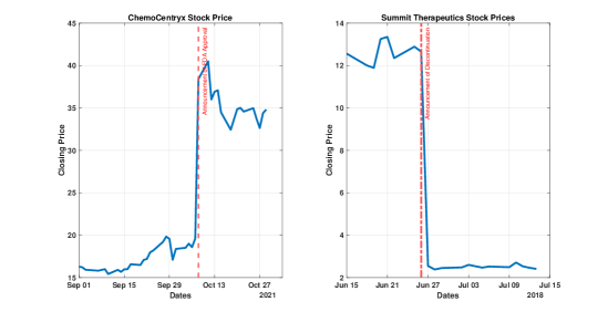
Note: Panels (a) and (b) display the time series of stock prices for ChemoCentryx pharmaceutical and Summit therapeutics around announcement dates, respectively. On October 8, 2021, ChemoCentryx announced FDA approval for its vasculitis drug. On June 27th, 2018, Summit announced the discontinuation of its Duchenne muscular dystrophy drug after the Phase II clinical trial.
In Figure 1-(b), we plot the share price of Summit Pharmaceuticals around a negative announcement. On June 27, 2018, Summit announced that starting June 26, 2018, it had discontinued the development of its Duchenne muscular dystrophy drug named ezutromid after the Phase II clinical trial, and the market responded negatively to this news.555Click here for Summit’s (archived) announcement document. Last accessed November 14, 2023.
Next, in Table 1, we present examples of five successful drugs, including information about the dates associated with three development milestones. We can determine the time it takes for a drug to reach the market, and in some cases, we also have sales data that will allow us to evaluate our estimates of drugs’ values. In the rest of the paper, we summarize institutional details and the data and formalize the idea that the change in a firm’s market value in a tight window around announcements identifies drug value and cost.
| (1) | (2) | (3) | (4) | (5) | |||||||||
|---|---|---|---|---|---|---|---|---|---|---|---|---|---|
| Drug Name | caspofungin |
|
evolocumab |
|
ziprasidone | ||||||||
| Firm | Merck & Co Inc | Biogen Inc | Amgen Inc |
|
Pfizer Inc | ||||||||
| Indication | Fungal Infection |
|
|
|
|
||||||||
| Discovery | Jun 12, 1996 | Nov 12, 2003 | Jun 16, 2009 | Feb 21, 2007 | Jan 1, 2002 | ||||||||
| FDA Application | Dec 13, 2000 | Feb 28, 2012 | Aug 28, 2014 | Mar 20, 2016 | Aug 31, 2003 | ||||||||
| FDA Decision | Jan 1, 2001 | Mar 27, 2013 | Jul 17, 2015 | Feb 28, 2017 | Aug 31, 2004 | ||||||||
| Sales (15 years) | $1.504 bil | $45.6 bil | $0.856 bil | $0.268 bil | $2.26 bil |
Note: This table displays key information for five successful drugs in our sample. For each drug, we observe its name, the firm developing the drug, the indication for which the drug is being developed, the dates for three stages of development, and discounted 15 years of sales revenue. The sales figures are real and expressed in December 2020 dollars.
3 Institutional Background and Data
3.1 Drug R&D and Announcements
The R&D process in the U.S. pharmaceutical industry consists of distinct stages defined by the FDA. Figure 2 is a schematic description of the drug development process. The first stage is a preclinical stage that includes creating a new molecule (or a system of molecules) and testing it (in vitro and in vivo) in the laboratory. We refer to this stage as “discovery.”
If successful, the firm can test the drug candidate in humans during three phases, known as clinical trials. In Phase I of the clinical trials, the firm screens the drug for possible toxicity using a small sample of healthy subjects. In Phase II, the firm tests the drug for efficacy on a larger sample with targeted diseases. Finally, in Phase III, the firm uses double-blinded tests to assess the drug’s effectiveness on a large sample.
Note: This is a schematic representation of the drug development process, where the entries “success” and “failure” correspond to possible announcements by a firm.
After the successful completion of clinical trials, the firm can apply for FDA approval. The FDA has a group of internal and external experts who review the results from clinical trials and the manufacturing capacity of the applicant firm before deciding to approve the application. If the FDA approves the drug, the drug is launched in the market.
However, only some drug candidates reach the market. In Table 2, we present transition probabilities based on the frequency distributions, assuming, for simplicity, that the transition probabilities are homogeneous across firms and diseases. On average, only about 11% of drug candidates are successful unconditionally. In contrast, 89% of drugs that apply for FDA approval are successful.666A drug can be developed concurrently for multiple indications–reasons a medication might be used–by more than one firm. We define an observation to be at the individual firm-drug-indication level. Our estimate of 10.8% is comparable to estimates from the literature (Paul et al., 2010; Hay et al., 2014; Mullard, 2016; DiMasi et al., 2016; Wong et al., 2019), which range from 8% to 13.8%. These averages do not account for differences in preclinical evidence about the mechanism of action or the firm’s expertise in an indication. Conditional transition probabilities are estimated as the share of drugs that reached the next stage out of all the drugs in the current stage. Thus, the conditional probability of a drug reaching Phase II clinical trials, given that it has reached Phase I, is the ratio of the number of drugs that have reached Phase II to those that have reached Phase I.
| Probability of Reaching a Stage | |||
|---|---|---|---|
| Stages | Marginal | Conditional | |
| Phase I Clinical Trials | 0.512 | 0.512 | |
| Phase II Clinical Trials | 0.319 | 0.624 | |
| Phase III Clinical Trials | 0.167 | 0.524 | |
| FDA Application | 0.121 | 0.723 | |
| FDA Approval | 0.108 | 0.890 | |
Note: The unit of observation is a development project, i.e., a specific firm-drug-disease combination, associated with at least one announcement. The column labeled Marginal denotes the shares of all the initiated development projects, and the column labeled Conditional denotes the shares of the development projects that made it to the next stage. For example, 16.7% of all projects reached Phase III, and conditional in reaching Phase II, 52.4% made it to Phase III.
Announcements. Three regulatory paradigms affect firms’ announcements about the success and failure of drug candidates as they transition through different development stages. First, the Security and Exchange Commission (SEC) requires all public companies to disclose all material information to their investors via the annual 10-K, quarterly 10-Q, and current 8-K forms. Regulation Fair Disclosure, instituted in 2000, requires publicly traded firms to disclose all material information on time.
Second, the FDA controls what a firm can and cannot announce about its drugs during development. For instance, the Food and Drug Administration Modernization Act of 1997 established the centralized registry https://www.clinicaltrials.gov, and firms must register clinical trials within 21 days of enrolling the first subject. The FDA also requires firms to disclose information about their clinical trials and their FDA application processes whenever relevant. Furthermore, these announcements cannot be materially misleading.
Third, under the Sarbanes-Oxley Act of 2002, the SEC monitors firms’ announcements about their FDA review process. Since 2004, the FDA can refer to the SEC if “in the normal course of their activities, they believe that a company may have made a false or misleading statement to the investing public.”
These regulations incentivize firms to inform the market and the general public correctly and promptly. Nevertheless, it is up to companies to decide what is material and what is not misleading. This ambiguity is more pronounced when the results from clinical trials are “small” and for large companies developing multiple drugs. In such cases, firms may either delay announcements or bundle negative announcements with positive announcements to try and “soften” the market reaction.
However, we remain agnostic about the incentives for bundling because we focus on days with only one announcement by a firm. Furthermore, we consider only major announcements that are most certainly material. In particular, we use the information only about discovery, whether a firm applies for FDA authorization to market the drug, the FDA’s decision, and discontinuations at different stages.
International Announcements. Although most announcements in our sample are made in the U.S. and involve the FDA, U.S. firms also market drugs elsewhere, e.g., in the E.U. and Canada. We use announcements in all of the “western” countries. They all have similar rules governing drug development and announcements; see Chapter 7 of Ng (2015).
For instance, the drug development process in the E.U. is generally similar to that of the U.S. (Van Norman, 2016). The FDA counterpart in the E.U. is the European Medical Association (EMA), which manages a centralized list of diseases. Firms seeking to develop drugs against those diseases must follow the centralized procedure for approval. Firms submit a single authorization application to the EMA, and the centralized procedure allows the marketing of a drug based on a single E.U.-wide assessment of the drug.
However, most drugs authorized in the E.U. are approved by the member states. When a company wants authorization to sell the drugs in several member states, it can apply for simultaneous approval in more than one member state if it has yet to be authorized anywhere in the E.U. The company can apply for this authorization to be recognized in other E.U. countries if authorized in one member state. Irrespective of the authorization routes, E.U. legislation requires that each member state apply the same rules regarding the authorization and monitoring of medicines. Thus, we expect U.S. subsidiaries operating in other Western countries to behave similarly to their parent companies in the U.S. We further assume that all drugs must go through the same stages across all countries.777This assumption, while reasonable for drugs, does not hold for Class III medical devices, e.g., coronary artery stents, where the E.U. has a less stringent approval system than the FDA (Grennan and Town, 2020). Henceforth, we use “FDA” as an omnibus term to refer to all relevant regulatory agencies.
3.2 Announcements Data
Our primary dataset on drug development comes from Cortellis, which is owned and managed by Clarivate Analytics. The database includes detailed information on more than 70,000 drug candidates in the development process worldwide. The database tracks each drug candidate’s progression through different development stages using information from academic peer-reviewed articles, patents, press releases, financial filings, presentations, conferences, and FDA submissions. Almost half of all announcements in our final sample are from press releases and corporate publications.
The database also contains information about every development milestone for all drugs in the development process. Notably, it records the date when the information about each milestone was announced, the drug’s names, the associated firm, and the target disease. The database is regularly updated by professional analysts working for Clarivate Analytics, who ensure the consistency and accuracy of the data.
| Announcements | Dates | Single Annoucement Dates | ||||
|---|---|---|---|---|---|---|
| N | % | N | % | N | % | |
| Discovery | 12,053 | 62.2 | 7,828 | 67.6 | 5,582 | 67.4 |
| Discontinued during Discovery | 1,083 | 5.6 | 552 | 4.8 | 266 | 3.2 |
| Discontinued during Phase I | 1,168 | 6.0 | 635 | 5.5 | 232 | 2.8 |
| Discontinued during Phase II | 1,648 | 8.5 | 910 | 7.9 | 414 | 5.0 |
| Discontinued during Phase III | 565 | 2.9 | 435 | 3.8 | 234 | 2.8 |
| FDA Application | 1,277 | 6.6 | 1,017 | 8.8 | 763 | 9.2 |
| Discontinued after Application | 98 | 0.5 | 84 | 0.7 | 49 | 0.6 |
| FDA Approval | 1,473 | 7.6 | 987 | 8.5 | 741 | 8.9 |
| Total | 19,365 | 100.0 | 11,576 | 100.0 | 8,281 | 100.0 |
Note: The table displays the count (and share) of different types of announcements. The column “Dates” refers to unique dates associated with announcements, and “Single Announcement Dates” refers to unique dates with a single announcement.
In Table 3, we show the number of different announcements in our sample. For almost 30% of the dates, firms make more than one announcement. In Table 4, we display the distribution of the number of announcements per day. The median number of announcements is 1, but there is a long right tail because the number of announcements depends on firms’ drug portfolios.
Due to data limitations, we do not use announcements about the start of clinical trials. The database provides information about the dates associated with the start and end of clinical trials, but usually not about the dates when the firm announces the results from the clinical trials. For example, a firm may reveal that it completed the Phase II clinical trial for a drug at a conference, but we may not know if this was the first announcement about Phase II results. Similarly, we may observe the start date of (for example) a Phase II clinical trial, but the firm may have already announced the date when disclosing Phase I results. We need the date the information was publicly revealed to determine firms’ market values.
| Announcements | Mean | Med | 90% | Std. Dev. | Min | Max |
|---|---|---|---|---|---|---|
| All | 1.67 | 1 | 3 | 2.24 | 1 | 88 |
| Discovery | 1.04 | 1 | 2 | 1.81 | 0 | 86 |
| Discontinued during Discovery | 0.09 | 0 | 0 | 0.62 | 0 | 20 |
| Discontinued during Phase I | 0.1 | 0 | 0 | 0.57 | 0 | 13 |
| Discontinued during Phase II | 0.14 | 0 | 0 | 0.74 | 0 | 29 |
| Discontinued during Phase III | 0.05 | 0 | 0 | 0.28 | 0 | 5 |
| FDA Application | 0.11 | 0 | 0 | 0.44 | 0 | 17 |
| Discontinued after Application | 0.01 | 0 | 0 | 0.11 | 0 | 6 |
| FDA Approval | 0.13 | 0 | 0 | 0.69 | 0 | 38 |
Note: Summary statistics for the number of daily announcements by type.
3.3 Market Value of a Firm
We observe daily returns for all biomedical and pharmaceutical companies publicly listed on U.S. stock exchanges from CRSP. We merge the stock market data with the Cortellis data by matching firms’ names. However, firms may change their names, merge with another firm, or be acquired by another firm. To keep track of unique firms, we use CRSP-generated permanent I.D. numbers. We match if any name the firm has had in its history (i.e., any name associated with the CRSP-generated permanent I.D.) matches the name in the Cortellis data, which results in an unbalanced panel structure.
We define the “market return” as the return on the CRSP value-weighted portfolio (including dividends). We use a firm’s market capitalization as a measure of its size. We determine each firm’s median real market capitalization across years. We use the December 2020 consumer price index to deflate all dollar amounts. Figure 3 shows histograms of firm sizes for different subsamples. Market capitalization exhibits a long right tail in the full sample of firms in Figure 3-(a). The vertical lines denote the 5th ($11.6 mm) and 95th ($6.2 bil) percentiles, respectively. Figures 3-(b) and (c) display the density of market capitalization of firms for those with market capitalization between the 5th and 95th percentiles of all firms, i.e., the “Middle 90%” sample, and for those below the 95th percentile, i.e., the “Bottom 95%” sample, respectively.
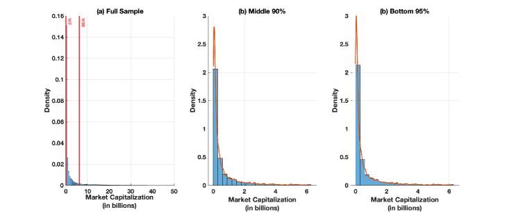
Note: The figure shows histograms of (real) market capitalization (in billions of U.S. dollars) of all the firms in panel (a), for the firms whose real market capitalization is between the 5th ($11.6 million) and 95th ($6.2 billion) percentiles in panel (b), and for the firms whose real market capitalization is below the 95th percentile in panel (c).
There is a long-standing comparison between the innovation performance of large and small firms; see Arrow (1983); Holmström (1989); Arora et al. (2009), and Akcigit and Kerr (2018). For our approach, heterogeneity between small and large firms can be crucial in several ways. Large firms might have more expertise and resources in conducting clinical development, increasing their chances of success and implying heterogeneity in transition probabilities. For the same reasons, large firms may conduct their clinical trials faster, implying differences in the time investors wait to realize their returns.
Similarly, because of the differences in scope from other firms, they may select and develop certain types of drugs (MCockburn and Henderson, 2001; Krieger et al., 2022). Finally, heterogeneity in market capitalization implies that an announcement about a drug with a specific value would result in a different percent change in the price of a single stock. Therefore, including large firms in our sample with all other firms may affect our estimates. So, in the empirical exercises below, we focus on the middle 90% and bottom 95% samples, although we also show the drug values estimated using the full sample.
4 Drug Valuation
To illustrate the main intuition behind our approach, let us re-consider the example mentioned in the introduction. Suppose a firm without any drugs in development announces the discovery of a new drug candidate to treat asthma. The product of the CAR and market capitalization (henceforth, mktcap) on the announcement day is the change in the firm’s market value. Because the only “news” that pertains to the firm was the discovery announcement, the change in the firm’s market value equals the expected net present discounted value of the asthma drug. The latter is the difference between expected revenue and R&D cost.
The expected net present discounted value of the drug at the time of discovery equals the discounted expected profit from the market adjusted for the probability that the drug will transition from discovery to FDA approval. A drug generates profits only after it is authorized to go on the market. However, the time of approval is uncertain (see Table (1) for examples). We use a stochastic rate to discount the expected stream of profits to the time of drug discovery. Ultimately, under the assumption that the expected profit is constant over time (ignoring any demographic shifts), we can express the expected net present discounted value of a drug as the product of (i) the present discounted profit from the market onwards, (ii) the probability that the drug will transition from discovery to the market, and (iii) the stochastic discount rate.
Next, suppose the firm initiates the FDA review process. At this stage, the market updates the expected value of the drug because even though the expected cash flow has not changed since the discovery announcement, the probability of FDA approval has increased. Moreover, the time until the drug may be authorized to enter the market is much shorter. Here, too, the product of CAR and mktcap at the time of announcement of FDA application is equal to the change in the probability of success times the drug’s expected profit discounted to the time of FDA application.
Finally, the FDA determines whether to approve the drug for distribution. If approved, all uncertainty surrounding the drug development process is resolved. The product of CAR and mktcap is equal to the product of the probability of failure and the expected present discounted sum of the variable profit.
The first step is to estimate the CAR associated with each announcement. Then, in the second step, we use a linear regression model to predict the CAR as a function of the announcement type. These predicted values for CAR, along with the mktcap, allow us to determine the expected change in the firm’s value immediately following an announcement.
4.1 Model
Let the random variable denote a firm’s market value and the firm’s development cost. There are three stages for which we have reliable data on the dates when an announcement was made: discovery, FDA application, and FDA decision, respectively, denoted by , and appr. We also have reliable data on drug discontinuations, denoted by drop. The cost is paid at different stages of development. To capture that, we use notations such as and to denote the cost from discovery to approval and from discovery to FDA application, respectively.
We begin by introducing some additional notation. Let denote the stage announcement about the success or failure of a drug, with the interpretation that denotes success in stage and denotes failure. Our sample starts from the discovery stage, so by definition, . For any two consecutive stages and , let denote the conditional probability that the drug is successful in stage , given that it is successful in the previous stage . For example, is the probability that a drug reaches the FDA application stage conditional on completing Phase III clinical trials. Likewise, is the probability that the firm discontinues before submitting an FDA application after finishing Phase III trials.
We now show how we can use changes in a firm’s market capitalization following an announcement about a drug to learn about the drug’s value. When a firm announces that the FDA has approved a drug, the firm’s value should jump immediately after the announcement, with the size of the jump equaling the increase in the expected profits from selling the drug. However, the only relevant change in the drug’s status since the last announcement is no more uncertainty about the development process. In other words, the value of the drug, which is the expected present value of market profits conditional on regulatory approval, equals the increase in the firm’s market value adjusted by the ex-ante probability of success. In particular, we have the following equation associated with announcements about FDA approval:
| (1) | |||||
Note that for notational ease, we suppress the dependence of the drug’s perceived market value (conditional on approval) on the information revealed during the review process. We estimate the ex-post value of a drug, , for each drug, so we can allow this value to depend arbitrarily on any information observed by the market. The only difficulty is that we, as researchers, do not observe such information. Thus, in principle, the FDA review process affects the transition probability and the value of the drug.
We can estimate the expected CAR using stock prices and announcements data, as we show later. Furthermore, we observe the market capitalization from CRSP. Substituting from Table 2 in (1), we can identify the value of a drug, at the time of approval. Notice that there is no cost at approval because the development costs would have been paid by then. The costs necessary to launch and market the drug are included in this estimate.
It is helpful to introduce new notation regarding discounting rates and profits. Let be the probability that a drug will get FDA approval within the next years conditional on reaching stage of development. For example, is the probability that a drug gets FDA approval in the next years, given that it has successfully submitted the FDA application. Hence, for all . Let be the annual discount factor, and let be the expected discount rate when the drug is at stage . In Section 5.3, we use a competing-risk model to estimate the time-to-success for all .
To help interpret the expected value of a drug at approval, we introduce new notation and make some simplifying assumptions. Let be the expected (average) yearly profit from selling the drug after FDA approval. The per-period profits do not include the sunk costs faced by the firm after the drug is approved but before it is marketed. Suppose the fundamental value of a drug is the same between discovery and approval. Then, the expected value of a drug is the present discounted profits, i.e., .
Furthermore, suppose the development announcements only affect the transition probabilities and time to success but not the perceived value of the drugs. So, the difference in the expected drug value at discovery and approval is entirely due to uncertainty about success and discounting. Then, we can show that, given the transition probabilities and the expected discount rate, we can estimate the expected value of the drug when the discovery announcement is made. The expected value at discovery is given by
| (2) | |||||
Therefore, to determine the value at discovery, we have to impose additional assumptions than we did to determine the value of successful drugs. The constant per period profit assumption simplifies the interpretation of the expected value and can be relaxed without affecting our procedure. However, the other assumption that development announcements do not affect the perceived value is strong, especially if the contents of the future announcements affect the market’s perception of the value of the drugs. To relax this assumption we need to keep track of the content of each announcement, which is infeasible with our current data and leave it for future research.
5 Cumulative Abnormal Returns and Discount Rates
Our event study methodology is based on estimating the impact of each drug development announcement on the value of a firm. If there is only one announcement, the change in the firm’s value, which we estimate, is also the expected net present value of the drug.
This relationship between the change in the firm’s value on the day of the announcement and the expected net present value of the drug continues to hold even when a firm is developing more than one drug so long as there is only one announcement on a given day. In this section, we formalize this idea and discuss estimating the expected discount rates.
5.1 Cumulative Abnormal Returns
In this section, we show how we estimate the cumulative abnormal return (CAR) associated with each drug-firm-announcement combination. CAR accounts for the effect of predictable variation in the firm’s value (using the market return) and cumulates over a window around the event to account for partial adjustment of stock prices to the new information.
Then, we use a linear regression model to decompose CAR as a function of different types of announcements, i.e., discovery, FDA application, FDA approval, and discontinuations at different stages. Using the estimated regression coefficients, we determine the expected change in the firm’s market value given an announcement and apply it to determine the value of drugs and the average cost of drug development using the method detailed in Section 4.
It is helpful to introduce some notation and then define CAR. Let denote the stock return of firm , at date and denote the market-wide return at date , which we proxy for using the return on the CRSP value-weighted portfolio for that day. Let denote the set of announcements by firm , and we let denote the date when firm makes its announcement. If the announcement date is not a trading day, denotes the first trading date after the announcement.
We use an unrestricted market model and posit that firm ’s log of returns () is a linear function of the log of the market return (), i.e.,
| (3) |
For each firm-announcement date pair , we determine for a 200-day window that ends ten days before the announcement date , and we fit (3) using linear regression.888Stopping ten days before the announcement lowers the chance of having the announcement and the lead-up to the announcement contaminate abnormal returns. We use a 200-day estimation sample to account for possible time variation in the relationship between a firm’s returns and market returns.
For each firm , we estimate as many of these regressions as the number of announcements in . From this estimation exercise, we obtain estimates of respectively, where we index the estimates with and to denote that these estimates differ by the firm and by the announcement. The abnormal returns associated with the announcement are then the fitted residuals from (3), i.e., .
Then the CAR associated with announcement , by firm on is the cumulative sum of around a pre-specified window and is given by
| (4) |
where and are the lower and upper window lengths of the event study, respectively.
For our estimation, we set and , which means we aggregate the abnormal returns one trading day before and two after the announcement. We estimate (3) for every firm-announcement pair separately and use the estimated to determine the associated CAR using (4). Table 5 reports the summary statistics of the CAR across all firms and all announcements. The average CAR has the expected signs: on average, the CAR is positive for good news and negative for bad news.
| Mean | Median | Std. Dev. | Min | Max | N | |
|---|---|---|---|---|---|---|
| Overall | -0.225 | 0.010 | 10.917 | -180.528 | 207.120 | 11,576 |
| Discovery | 0.221 | 0.031 | 9.105 | -137.464 | 165.573 | 7,828 |
| Discontiued During Discovery | -0.159 | 0.314 | 10.915 | -126.511 | 57.733 | 552 |
| Discontinued During Phase I | -1.333 | -0.097 | 12.964 | -124.009 | 66.176 | 635 |
| Discontinued During Phase II | -4.002 | -0.513 | 18.911 | -175.680 | 66.176 | 910 |
| Discontinued During Phase III | -6.556 | -0.377 | 24.213 | -180.528 | 36.380 | 435 |
| FDA Application | 0.290 | 0.154 | 6.913 | -44.419 | 116.284 | 1,017 |
| Discontinued After Application | -0.667 | -0.007 | 8.014 | -43.724 | 18.584 | 84 |
| FDA Approval | 1.039 | 0.291 | 9.793 | -68.960 | 207.120 | 987 |
Note: Summary statistics for CAR as defined in (4), by each type of announcement.
We observe that the magnitude of positive and negative announcements increases as we progress in the development process. For example, the average CAR associated with FDA approval is larger than that associated with FDA applications or discovery announcements. This pattern is consistent with the fact that in the later stages of development, the higher the chance of success, the smaller the remaining development costs, and the sooner the launch. A mean CAR of for Discovery announcements means that, on average, a firm’s share price increases by 22 basis points after announcing the discovery of a new drug. The interpretation for other types of announcements is similar. Overall, these estimates suggest that the release of clinical trial results is an economically significant event and has meaningful effects on market value. However, negative news (discontinuation) has a larger effect than positive news. This asymmetry in the market’s reaction has been previously noted by Hwang (2013) and Singh et al. (2022).
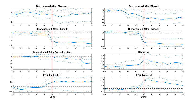
Note: The figures display CAR, expressed in percentage points on the y-axes, for a ten-day window around the event day (denoted as 0 and marked by red vertical lines), with a 90% confidence interval. Each figure corresponds to the type of announcement. We use those events with one announcement.
One concern with the announcements is possible information leakage before the official announcement. Figure 4 investigates the possibility of such leakage in our sample. Each panel corresponds to a different type of announcement. The x-axis denotes event time, where 0 corresponds to the day an announcement occurred. Negative numbers are the days leading up to the announcement, and positive numbers are the days after. The y-axis measures CAR in percentage points. The solid blue line is the average CAR across all announcements of the specified type from 10 days before to 10 days after the announcement, the dotted blue lines are 90% bootstrapped confidence intervals, and the dotted black line is at 0.
According to the efficient markets hypothesis, we would only expect a non-zero CAR on an announcement day because of the new information about the prospects of the relevant drug, e.g., increased probability of success. We would also expect the CAR to “jump” at time 0. Systematic increases or decreases in the CAR before an announcement suggest information leakage. The figure shows that the CAR in the days leading up to the announcements is statistically insignificant. There is little evidence of information leakage across announcement types, as all the panels suggest that the primary change in CAR occurs on the day of the announcement.
If a firm develops more than one drug simultaneously, it may make multiple announcements about different drugs on the same day. In such cases, all the announcements have the same CAR, and we cannot separate the effect of each announcement on CAR. So, throughout the paper, we focus only on dates associated with single announcements.
5.2 Effects of Announcements on CAR
From Table 5, we see that the type of announcement affects the CAR. Instead of using the sample mean of the CAR, we use OLS by pooling across all firms, drugs, and time to determine the marginal effects of different types of announcements on CAR, assuming that the effects are homogeneous across firms and drug candidates.
In particular, to determine the expected CAR for each type of announcement, we use the following linear model
| (5) | |||||
where the dependent variable is from (4), and discontinuations is a vector that includes separate indicators for discontinuation during discovery, Phase I clinical trials, Phase II clinical trials, Phase III clinical trials, and FDA applications. For example, if firm ’s -th announcement was made on date and if the announcement was the discovery of a drug, is equal to 1 and the other right-hand-side variables in (5) for are zero.
Thus, each coefficient measures the marginal effect on the average CAR of a specific announcement. For instance, is the change in expected CAR associated with the announcement that a firm has applied for FDA approval. The estimated coefficients from (5) are in the first column (full sample) of Table 6. To capture the uncertainty in the estimated coefficients, particularly the error in the estimation of , we also present the 90% bootstrapped confidence intervals based on 1,000 bootstrap samples. The coefficients have the expected signs in line with our results for average CAR in Table 5.
| Full Sample | Middle 90% | Bottom 95% | |
| Discovery | 0.213 | 0.37 | 0.401 |
| [0.029, 0.420] | [0.029, 0.420] | [0.029, 0.420] | |
| Discontinued during Discovery | -0.921 | -2.429 | -2.43 |
| [-2.239, 0.255] | [-2.238, 0.254] | [-2.238, 0.254] | |
| Discontinued during Phase I | -1.150 | -2.33 | -2.319 |
| [-2.191, -0.157] | [-2.191, -0.157] | [-2.191, -0.157] | |
| Discontinued during Phase II | -3.637 | -7.63 | -7.813 |
| [-5.199, -2.252] | [-5.198, -2.252] | [-5.198, .2.252] | |
| Discontinued during Phase III | -7.310 | -15.8 | -15.809 |
| [-9.963, -4.626] | [-9.962, -4.625] | [-9.962, -4.625] | |
| FDA Application | 0.496 | 0.672 | 0.683 |
| [0.047, 0.953] | [0.047, 0.953] | [0.047, 0.953] | |
| Discontinued after FDA Application | -1.384 | -3.451 | -3.451 |
| [-3.736, 0.850] | [-3.736, 0.849] | [-3.736, 0.849] | |
| FDA Approval | 1.158 | 4.017 | 4.017 |
| [0.547, 1.836] | [0.546, 1.836] | [1.836, 1.985] | |
| Observations | 8,281 | 3,968 | 4,032 |
| 0.021 | 0.047 | 0.048 |
Note: The table presents estimated coefficients from Equation (5) using only single announcements. Each coefficient is followed by a 90% bootstrap confidence interval estimated using 1,000 bootstrap samples.
Consider the following example to help interpret the coefficients from the regression. Suppose a firm with a market value of $100 mm announces discovering a new drug compound. After the announcement, its market value is, on average, mm.
In columns two and three of Table 6, we present estimates using the middle 90% and bottom 95% samples. While the estimates for these samples have the expected signs, compared to the full sample, we find that these restricted samples have larger estimated effects for all announcements. However, the discontinuations have particularly larger negative effects. These estimates are consistent with, all else equal, announcements having larger effects on smaller firms than larger ones, and the theory (Shin, 2003) that predicts that the return variance following a poor disclosed outcome is higher than it would have been if the disclosed outcome were good.
5.3 Expected Discount Rates
In this section, we present the estimates of discount rates for different stages. As we showed earlier in (2), to determine the expected value of a drug at discovery, , we begin with its value at approval, . Then, we discount it to the discovery stage using transition probabilities and the discount rate , where the expectation is taken at discovery with respect to the distribution of the time for FDA approval.
Let denote the probability that a drug will move to phase I clinical trials by year given that it is starting at the discovery stage. Suppose we know and all subsequent development-stage time probabilities. In that case, we can determine the probability of time to success from discovery to FDA approval, denoted by . Then we can estimate the expected discount rate using Monte Carlo simulation, i.e., , where is the time it takes for a drug to get approval from discovery. Therefore, to estimate the expected discount rate, we have to estimate the probabilities of time to success for all five stages.
To estimate the probabilities, we follow Aalen (1976) and use the observed time it takes for drugs to transition to the next stage (which we call “success”). Figure 5 shows the histograms of time (in years) it takes to move to the next stage–time to success–or discontinuation. Thus, there are “competing risks” at any time; a drug can be in its current state until it is either discontinued or succeeds and moves to the next stage. We refer to these three states as status-quo, failure, and success by , respectively. The idea is the same for and , except now we start from clinic and appl, respectively.
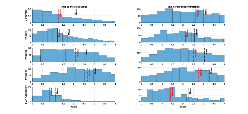
Note: Histograms of the time (in years) it takes for drugs to transition to the next stage, i.e., time to success, are in the first column, and when drugs are discontinued, i.e., time to failure, are in the second column. Each row corresponds to one stage, starting from Discovery in the first row to FDA application in the last. The two vertical lines denote the mean (in black) and the median (in red) of the time for that stage and event. The x-axes have been limited to only four years for easy presentation.
Let denote the probability that a drug stays in the state at time given that it started at state at time . The probability of transition from state to state by time is given by
Next, let and be the number of drugs in the development stage and for which the firms applied for approval at time , respectively. Suppose that we partition into small intervals such that there is at most one transition in each subinterval. In an interval , the conditional probability of one transition from development to FDA application, given that there are drugs in the development stage, is equal to . Thus, if there is only one transition, we can estimate the transition probability by . Aalen (1976) shows that this intuition applies more generally and that we can estimate the hazard rate that defines above by
In practice, we apply this method separately to five different subsamples: (i) drugs at the discovery stage, where the failure is discontinuation and the success is the transition to Phase I clinical trial; (ii) drugs in Phase I clinical trials where a failure is a discontinuation and the success is the transition to Phase II clinical trial; (iii) drugs in Phase II clinical trials, where the failure is discontinuation, and the success is the transition to Phase III clinical trial; (iv) drugs in Phase III clinical trial, where failure is discontinuation, and success is FDA application; and (v) drugs after FDA application, where success is FDA approval. These five exercises give us the transition probabilities. Using these estimates, we determine the expected discount rates using , which are in Table 7.
| Full Sample | Middle 90% | Bottom 95% | |
|---|---|---|---|
| Discovery | |||
| Discovery to Phase I | 0.820 | 0.821 | 0.823 |
| Discovery to Phase II | 0.733 | 0.737 | 0.738 |
| Discovery to Phase III | 0.608 | 0.637 | 0.637 |
| Discovery to FDA Application | 0.507 | 0.554 | 0.555 |
| Discovery to Market | 0.448 | 0.482 | 0.483 |
| Clinical Trials Phase I | |||
| Phase I to Phase II | 0.893 | 0.897 | 0.897 |
| Phase I to Phase III | 0.740 | 0.775 | 0.775 |
| Phase I to FDA Application | 0.618 | 0.674 | 0.675 |
| Phase I to Market | 0.546 | 0.586 | 0.587 |
| Clinical Trials Phase II | |||
| Phase II to Phase III | 0.828 | 0.863 | 0.863 |
| Phase II to FDA Application | 0.692 | 0.751 | 0.752 |
| Phase II to Market | 0.611 | 0.653 | 0.655 |
| Clinical Trial Phase III | |||
| Phase III to FDA Application | 0.835 | 0.870 | 0.871 |
| Phase III to Market | 0.737 | 0.756 | 0.757 |
| FDA Application | |||
| FDA Application to Market | 0.883 | 0.869 | 0.870 |
Note: Expected discount rates for different stages are estimated using competing risk models, with a yearly discount rate of 0.98. The columns use full sample, middle 90% sample, and bottom 95% sample, respectively.
6 Drug Values
In this section, we use the estimates in the third column of Table 6 combined with regression Equation (5) to determine the change in the market value of a firm associated with each announcement. Then, we apply the methodology presented in Section 4 to determine the value of a drug and the average cost of drug development. Thus, we first consider the case of homogenous expectation across all diseases. Then, we consider the heterogeneous case and estimate the values separately for 11 major diseases.
6.1 Homogenous Case
To determine the expected value of drugs at approval, i.e., , we use all drugs that reach the market in Equation (1). Figure 6 shows the histograms of the expected drug values measured in billions of dollars for the sample of drugs for which firms submitted applications for FDA approval.999We could also use announcements about discontinuations after FDA application to inform the estimates of drug values. However, there are only a few such announcements, and the CAR estimate associated with that event is noisier, so we do not use them to estimate drug values.
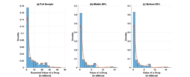
Note: The figure shows histograms and densities of (in billions of US dollars) for drugs with FDA approval. Panel (a) corresponds to the full sample (1,561 drugs received FDA applications); Panel (b) corresponds to the middle 90% sample (378 drugs), and Panel (c) corresponds to the bottom 95% sample (401 drugs). To calculate values, we use the transition probabilities from Tables A.1, effects of announcements on CAR from Table 6, and the discount rates from Tables 7.
Figure 6-(a) considers only the drugs that received FDA approval in the full sample. There are 1,561 such drugs, and we can use Equation (1) to identify their values. The estimated drug values range from $110,300 to (approximately) $45.8 billion, with a mean of $6.83 billion and a standard deviation of $8.88 billion. Column 1 of Table 8 reports the two estimates for the mean expected value at approval is $6.83 billion.
In light of the pronounced right skewness in the firm size distribution, we estimate the value of drugs after removing the outlier firms. The data restrictions are motivated by our discussion of the distribution of market capitalization in Section 3.3. We are concerned that large and small firms are fundamentally different from other firms. So, we remove firms with a market capitalization of either less than the 5th or more than the 95th percentile. We call this sample “middle 90%.” We also consider the sample where we remove large firms with a market capitalization larger than the 95th percentile. We call this sample “bottom 95%.”
We separately estimate transition probabilities, discount rates, and Equation (5) for these indications. The estimates from CAR regressions are in Table 6, the expected discount factors are in Table 7, and the transition probabilities are in Table A.1. Figures 6-(b) and (c) show the histograms of valuations of successful drugs for the middle 90% (378 drugs) and bottom 95% samples (401 drugs). Unlike the full sample, these samples have fewer outliers.
The estimated values are in Table 8. We find that the mean of the expected values is $1.62 billion among the 378 drugs developed by mid-90% firms, which is smaller than in the full sample. For the bottom 95% sample, the average value of a drug is $1.6 billion.
| Full Sample | Middle 90% | Bottom 95% | |
|---|---|---|---|
| At Approval | |||
| All Drugs | $6.83 bil | $1.62 bil | $1.6 bil |
| Drugs with Complete Path | $7.43 bil | $1.89 bil | $1.99 bil |
| At Discovery | |||
| All Drugs | $331.12 mm | $63.37 mm | $65.97 mm |
| Drugs with Complete Path | $360.16 mm | $74.05 mm | $82.21 mm |
Note: The table presents the mean of the expected value of individual drugs at the time of approval, , and at discovery, . The 90% sample refers to the drugs developed by firms with real market capitalization between 5% and 95% of the entire sample. The row, “Drugs with Complete Path” refers to the sample of drugs for which we observe discovery, FDA application, and FDA approval announcements. Of the 84 drugs, 29 belong to the Middle 90% The row “Average” refers to drugs for which we observe only a few stages.
For a subsample of 84 drugs, we observe the “complete path” from discovery to FDA approval, and we can determine their values and costs without combining estimates across other drugs for which we do not observe complete paths. Although we prefer to use all the drugs, we also consider this particular subsample of drugs for sensitivity analysis and present the estimates in Table 8 in the row labeled “Drugs with Complete Path.” The estimated values of 29 drugs with complete paths at $1.89 billion and $1.99 billion are similar to the estimates associated with all approved drugs for the middle 90% and bottom 95% samples, respectively.
Once we have the expected value of the drug at the time of approval, we can also determine the value at the time of discovery using Equation (2). In particular, the value at discovery is the value at approval adjusted for the likelihood of a drug getting approval and discounted to discovery. These estimates are shown in the second half of Table 8. Using the entire sample, we estimate the expected value at discovery to be $331.12 million. When we consider the middle 90% and bottom 95% samples, the mean of the expected value at discovery is $63.37 million and $65.97 million, respectively.
To verify that the magnitude of the estimated values is reasonable, we have collected additional data on sales. The expected value is the NPV of the cash flow that accrues to the firm, so our estimates should be similar to what we would get from discounted sales data.
We use sales data from the Cortellis Competitive Intelligence database, which includes information on yearly drug-level total (worldwide) sales. The data were obtained from firms’ SEC filings and are relatively sparse.
The sales data are at the drug level, but the announcements are at the drug-disease level. We do not observe the breakdown of sales by disease, so we allocate the sales equally across all diseases associated with the drug. So, if a drug targets three conditions, each would be assigned one-third of the total sales.
| Variable | N | Mean | Median | Std. Dev. | Min | Max |
|---|---|---|---|---|---|---|
| Full Sample | ||||||
| Average yearly sales | 764 | 268.24 | 69.90 | 519.57 | 0.10 | 6,655.11 |
| # of years data available | 764 | 11.57 | 10 | 8.84 | 1 | 34 |
| Middle 90% and Bottom 95% | ||||||
| Average yearly sales | 148 | 155.79 | 32.94 | 317.31 | 0.10 | 1,791.74 |
| # of years data available | 148 | 6.50 | 5 | 5.97 | 1 | 23 |
Note: Sales (in millions of U.S. dollars) data on the firm-drug-disease level.
Table 9 presents the descriptive statistics for the sales data. Typically, the data are available for only about ten years, which is short for pharmaceutical sales, as many drugs stay on the market for over 20 years. To correct the short panel duration, we average sales across all the years available for a given drug-and-disease pair for a given firm. Assuming that this average sales value is received yearly, we calculate the discounted total sales for this drug-disease-firm pair.101010For example, suppose we observe sales for Wyeth’s insomnia drug called Zaleplon for three years. The sales data for these three years are $54 million, $133 million, and $109 million (in 2020 U.S. dollars). The average sales value is then $(54+133+109)/3=$98.7 million. We then use these average sales to calculate the total discounted sales for a time horizon of length employing as .
Table 10 presents the results for different time horizons after aggregating average sales. We find that the total discounted sales of the drug if the drug had been in the market for ten years is $2.4 billion for the full sample and $1.4 billion for the middle 90% and bottom 95% samples. Considering that generic drugs may drive the prices down, the observed sales presented in Table 10 support our approach to estimating the expected value of a drug.
| Sample | 10 yrs | 15 yrs | 20 yrs | 25 yrs | 30 yrs |
|---|---|---|---|---|---|
| Full Sample | $2.4 bil | $3.44 bil | $4.37 bil | $5.21 bil | $5.97 bil |
| Middle 90% and Bottom 95% | $1.4 bil | $1.99 bil | $ 2.54 bil | $3.03 bil | $3.47 bil |
Note: Each entry shows total discounted sales averaged across drug-firm-diseases for a specific time horizon. The Full Sample refers to those drug-firm-diseases for which we have the sales data and are also present in our Full Sample for the value estimation. Middle 90% refers to those drug-firm-diseases present in the Middle 90% sample for the value estimation (drugs developed by firms whose real market capitalization is between 5% and 95% of the entire sample).
6.2 Heterogeneous Case
The estimates so far are based on homogeneous transition probabilities and distributions of the time to success. The transition probabilities in Table 2 are consistent with the averages in the literature (e.g., Hay et al., 2014), but they likely also vary across diseases (or indications) (e.g., Wong et al., 2019). For instance, the likelihood of developing a successful drug for neoplastic illnesses, which include cancer, is likely different from endocrine diseases, which include diabetes. If so, all else equal, an announcement (e.g., FDA approval) should have other effects on the firms’ values depending on the relevant indications.
However, our approach can be readily adapted to capture heterogeneity across diseases. In particular, we consider 11 major indications and, for each, estimate the valuations at FDA approval and discovery following the same steps as in Table 8. An indication is the most aggregated level of disease classification available in our sample. From the list of 34 indications, we chose 11 major indications that have sufficiently many (approximately 1,000) announcements. These indications are listed in Table 11.
For each indication, we estimate the expected cumulative abnormal returns using (5), transition probabilities, and distributions of time to success. To keep the exposition shorter, we do not present the estimates from the regression and focus only on the full sample and the middle 90% sample, but not the bottom 95% sample.
Table A.2 in the appendix presents the estimated transition probabilities from the discovery stage to the market and from FDA application to the market, separately for each indication. As before, the ex-ante probability that a drug is successful is small and differs across indications. For instance, the probability of developing a successful cure for neoplastic diseases is 9% and 16% for endocrine diseases. Conditional on reaching the FDA application stage, the likelihood is high, and these probabilities differ across indications. Table A.3 presents the expected discount rates from discovery to market.
Using these estimates in Equation (1), we determine the expected value of drugs at approval, i.e., , for each indication, and then using Equation (2) determine the expected value of drugs at discovery, i.e., . In Table 11, we present the average values of drugs (in billions of US dollars), where the averages are taken across all drugs within an indication.
| Indications | Full Sample | Middle 90% | ||
|---|---|---|---|---|
| Approval | Discovery | Approval | Discovery | |
| Cardiovascular diseases | $4.96 | $0.26 | $4.01 | $0.25 |
| Endocrine diseases | $11.40 | $1.10 | $15.30 | $1.40 |
| Gastrointestinal diseases | $2.26 | $0.17 | $0.87 | $0.05 |
| Hematological diseases | $11.60 | $1.28 | $6.06 | $0.56 |
| Immune disorders | $22.60 | $1.68 | $40.60 | $2.74 |
| Infectious diseases | $0.91 | $0.09 | $-0.40 | $-0.02 |
| Inflammatory diseases | $5.45 | $0.34 | $6.84 | $0.35 |
| Musculoskeletal diseases | $16.00 | $1.71 | $7.85 | $0.69 |
| Neoplastic diseases | $3.32 | $0.18 | $2.66 | $0.09 |
| Neurological diseases | $8.07 | $0.41 | $2.63 | $0.19 |
| Rare diseases | $15.30 | $1.90 | $7.83 | $0.82 |
Note: The table presents the mean of the expected value of individual drugs (in billions of US dollars) at the time of approval, , and at discovery, , for 11 indications. The 90% sample refers to the drugs developed by firms with real market capitalization between 5% and 95% of the entire sample.
As seen, the average values of drugs differ significantly across indications. For instance, the average value of medicines for infectious diseases is (numerically) zero. This estimate is consistent with the fact that infectious diseases include bacterial infections, such as Pneumonia, Sinusitis, and urinary tract infections, treated with antibiotics that tend to have small values. See, for example, Missialos et al. (2010). On the other hand, the value of approved drugs that treat immune disorders, which include type 1 diabetes, is $40 billion. At the discovery stage, the average value is $2.74 billion. The value of drugs at discovery is substantially smaller across all indications, underscoring the ex-ante risk of developing drugs.
7 Application of the Estimates
Next, we consider two applications for our method. First, we extend our approach and use the valuations to determine the cost of drugs R&D. Second, we investigate a broader context for the estimates of drug innovation and how policymakers might use them to incentivize drug development, given that these estimates reflect the existing economic and regulatory environment. For ease of presentation, we only consider the homogenous case (Section 6.1).
7.1 Cost of Drug Development
Here, we show that under some additional assumptions about information and timing of announcements, we can extend our approach to estimate the mean costs of drug development at different stages using the effects of discontinuation announcement on a firm’s value. Most drugs do not succeed and are discontinued at different stages of the development process. If the firm announces that it is stopping the development, the product of the CAR and the mktcap should be negative, reflecting the decrease in the firm’s value following this “bad news.” This change in the firm’s market value is informative about the remaining expected development cost.
Once we have , we can use the discovery announcements to infer the expected development cost from discovery to FDA approval, i.e., . In particular, the change in the market value of a firm immediately following a discovery announcement is equal to the difference in the expected value of a drug at discovery and the expected cost of drug development from discovery until FDA approval. Hence, we get
| (6) |
which then we can use to estimate .
To evaluate the costs associated with each stage of drug development separately, we use negative announcements about discontinuations at these different stages (see Table 3). We assume that, on average, there is no negative selection between discontinued drugs and their (ex-ante) profitability. This assumption is reasonable because the primary reason for discontinuations is negative clinical trial results (DiMasi, 2013; Khmelnitskaya, 2022).
Let us consider identifying the costs of FDA application and FDA review. We defer the discussion of what is included in the costs for FDA review to Section 7.1. We can use discontinuation announcements after Phase III clinical trials to identify these costs. The intuition is as follows. Following a discontinuation announcement, the firm’s market value falls by the amount the market expected the drug to earn (during the previous successful announcements) and increases by the cost savings that need not be incurred.
More formally, we begin with the following relationship:
| (7) |
Then, we note that the expected value of a drug at Phase III is given by , where all the variables on the RHS are known. Then, plugging this back in (7) we can identify .
Although we do not show the derivations here, following similar steps, we can use discontinuations at earlier stages to identify the expected costs of Phase I, II, and III clinical trials using discontinuation announcements after discovery and Phase I and II clinical trials, respectively. Furthermore, we note that to identify the costs of earlier stages of development (for example) Phase II clinical trials, we rely on our estimates of values, transition probabilities, and the discount rates and the estimated costs of later stages, e.g., Phase III clinical trials, FDA application, and FDA review.
Total Cost at Discovery. Next, we present the estimate of the expected total development cost at discovery, which includes the expected costs of clinical trials, FDA application, and the FDA review process. We use Equation (6) for that. In particular, by averaging both sides of (6) and substituting the average of the expected value of drugs at discovery, we can determine the expected cost of drug development at discovery for the middle 90% sample to be $58.51 million, and for the bottom 95% sample, $60.72 million.
| Middle 90% | Bottom 95% | |
|---|---|---|
| All Drugs | $58.51 mm | $60.72 mm |
| Drugs with Complete Path | $69.24 mm | $77.01 mm |
Note: The table presents the mean of the expected cost of clinical trials and the FDA application and review process (in millions of U.S. dollars) at the time of discovery. The 90% sample refers to the drugs developed by firms with real market capitalization between 5% and 95% of the entire sample. The row “Drugs with Complete Path” refers to the sample of drugs for which we observe discovery, FDA application, and FDA approval announcements. There are 84 such drugs, out of which 29 belong to the Middle 90% and Bottom 95% samples. The row “Average” refers to drugs for which we do not observe the complete path but only a subset.
Notice that this cost is the risk-adjusted cost at the time of discovery. In other words, this cost incorporates the risk that, with a high probability, the drug will not make it to the later, more expensive stages of development.
Cost of the FDA Review Process. Next, we use Equation (7) associated with discontinuations after Phase III clinical trials to estimate the expected cost of FDA application and review. Although the scientific experiments are mostly completed at the time of application, there would still be additional expenses to set up manufacturing capacity and legal and administrative fees.111111The FDA has prepared a set of instructions for drugs to receive approval. The instructions in Food and Drug Administration (2010) clarify that the “FDA may approve an NDA or an ANDA only if the methods used in, and the facilities and controls used for, the manufacture, processing, packing, and testing of the drug are found adequate to ensure and preserve its identity, strength, quality, and purity.”
The estimates are presented in Table 13. We estimate the expected cost to be $638.75 million for the middle 90% sample and $648.04 million for the bottom 95% sample. This cost estimate should be interpreted as the remaining cost the firm must face between when the application to the FDA is submitted and when the drug is approved.
| Middle 90% | Bottom 95% |
| $638.75 mm | $648.04 mm |
Note: The table presents the mean of the expected cost of FDA review and FDA application at the time of discovery. The middle 90% sample refers to the drugs developed by firms with real market capitalization between 5% and 95% of the sample.
Clinical Trials. The last step is determining the costs the firm expects to pay for the clinical trials. To determine these costs, we can follow the steps outlined in Equation (7) and present the results in Table 14. Specifically, using the discontinuation announcements after discovery, we estimate the expected cost of Phase I clinical trials for the two samples to be $620,510 and $219,240, respectively. The costs for Phase II clinical trials are substantially higher at $30.48 million (middle 90%) and $34.46 million (bottom 95%). To estimate these costs, we use the discontinuation announcements after Phase I. Similarly, using the discontinuation announcements after Phase II, we estimate the cost of Phase III clinical trials to be $41.09 million (middle 90%) and $39.71 million (bottom 95%).
| Middle 90% | Bottom 95% | |
|---|---|---|
| Phase I | $0.62 mm | $0.22 mm |
| Phase II | $30.48 mm | $34.46 mm |
| Phase III | $41.09 mm | $39.71 mm |
Note: The table presents the mean of the expected cost of the three phases of clinical trials. The middle 90% sample refers to the drugs developed by firms with real market capitalization between 5% and 95% of the entire sample.
Using these estimates of the costs of clinical trials, the transition probabilities (Table A.1), and expected discount rates (Table 7), we can determine the expected cost of running clinical trials where the expectation is at the time of drug discovery. We estimate the average cost of running clinical trials to be $11.8 million for the mid 90% sample and $12.43 million for the bottom 95% sample.
Cost Estimates in the Literature. It is helpful to compare our costs with prior estimates from the literature. For example, suppose we use the estimates of the transition probabilities, average durations for each phase, and average costs for each stage from DiMasi et al. (2016). In that case, the discounted expected cost of clinical development will be approximate $51.2 million (in December 2020 US dollars). While this estimate is larger than the comparable estimate of $11.8 million we get using our preferred specification, estimates from DiMasi et al. (2016) are known to be larger than even other estimates in the literature (Wouters et al., 2020).
However, Sertkaya et al. (2014) suggest that the cost of bringing a new drug to a market is between $161 million and $2 billion. Relatedly, using proprietary cost data on a small sample of drugs developed from 2004 to 2012, Sertkaya et al. (2016) estimate the average non-risk-adjusted (accounting) costs of the three phases of clinical trials range from $1.82 million to $8.58 million, $9.1 million to $25.48 million and $14.95 million to $68.77 million (in December 2020 US dollars), respectively. Finally, for drugs entering human clinical trials for the first time between 1989 and 2002, Adams and Brantner (2006) estimate the cost per new drug to be $868 million.
7.2 Drug Buyouts.
Here, we consider the possible use of our estimates by a government that wants to “open innovation” via drug buyouts and would do so by buying drugs and putting them in the public domain. We consider drug buyouts at two stages of development: (i) after FDA approval and (ii) at the discovery stage. Although the current system is not geared for drug buyouts, our analysis is motivated by similar considerations as Kremer (1998) and the recent debate surrounding the Medicare Drug Price Negotiation program of the Inflation Reduction Act 2022. We also consider the government adopting a cost-sharing strategy to support innovation by paying for development costs.
7.2.1 After FDA Approval
We first consider the case of the government buying out a drug right after FDA approval. After FDA approval, all uncertainties associated with the development of the drug are resolved, and all major R&D costs are sunk. Thus, the only question left is determining the drug’s final price.
As mentioned in the introduction, a key concern for any action taken by policymakers based on our estimates is Lucas critique: as the regulatory environment changes, agents re-optimize and change their decisions, possibly nullifying the intervention.121212 We sidestep the possibility that drug buyouts may also increase the “government-induced risk” in the industry (Koijen et al., 2016), which may affect firms’ decisions to participate in the program.
To make progress and to understand how this market feature may constrain the drug buyout policy, let us begin by sidestepping Lucas critique and assuming that the government offers to buy the drug at the value we estimated using Equation (1).
Our methodology provides a straightforward way to use the observed CAR (following the FDA approval announcement) and the market capitalization of the firm that developed the drug to learn the value of the drug up to the estimated transition probability. For example, suppose the CAR associated with FDA approval is 1%, the market capitalization is $1 billion, and the transition probability from FDA application to FDA approval is . Then, under the weak efficient market hypothesis, the value of the drug is million. In this example, the government would offer to pay $100 million for this drug, and the firm would agree to sell the drug.
If the government uses our procedure, our estimates (Table 8) suggest that on average, it will pay $1.62 billion per drug buyout.131313For all cases considered here, we use estimates from the middle 90% sample with all drugs and focus only on average costs and values for homogenous case, but our message extends to any of our other estimates.
The problem becomes nuanced once we factor in the Lucas critique. Once the market knows that the government will buy the drug, it will “bid” the value of the drug up to the amount investors expect the government to pay, which we take to be the social value.
For example, consider a drug with (unobserved) market value , and social value . The government still needs to learn the market value, but the social value of the drug is common knowledge. If, before FDA approval, the government announces that it will buy the drug, then, when the firm announces FDA approval, the market reacts to $500 and not $100.
Next, suppose the government waits until after FDA approval to announce that it wants to buy the drug. Then, the (unobserved) market value will be revealed when the FDA approves the drug. At this point, the government can make a take-it-or-leave-it offer to buy the drug at market value. However, this approach has a major drawback. It can be only a one-off intervention, for if the market expects that the government might buy the drug, investors will bid the value of the drug to and hedge their positions. They could do this by, for example, using put options to be exercised if the drug gets approved by the FDA and the government does not buy it. More generally, the government will affect market behavior (i.e., reactions) and, consequently, the estimates of the market value of the drugs.
Noticeably, paying a markup over the estimated market value, as suggested by Kremer (1998) for patents, i.e., paying , does not work either because there too, the market can “manipulate” the final payment by reacting to the total payout and not the “true” value. In conclusion, with these drug buyout interventions, we cannot use market reactions to FDA approval announcements to determine the market value of a newly approved drug.
To deal with Lucas critique, drug buyouts must be designed to prevent the market from anticipating the government’s decision and bidding up the value of the drug. We now propose a solution that does not require the government to commit to an offer, making it unprofitable for investors to hedge their positions.
We propose that the government announces that it will buy a drug with a small exogenous probability at the social value, , and both are common knowledge. Then the expected value of the drug is . Essentially, the government chooses the probability that it will buy a drug rather than the market determining it. Under the proposed solution, the government will pay the social value with probability . Then, adapting (1) to the new expected value, we can identify the market value of the drug.
There is also a more involved solution based on the same idea, but it can lower the cost of drug buyouts. In particular, the government can announce buying the drug at some , with . The market values of drugs tend to be substantially smaller than their social values, so the government may use our estimates of values to choose .
To see how the government can use our estimates to choose , let denote the distribution of the market value of drugs in Figure 6. The expected savings from offering instead of , for a fixed , would be , where is the probability that the drug’s market value is smaller than the offered . In other words, it is the probability that the firm will accept the offer. Then, the offer () that maximizes the expected savings is determined by , where the left-hand-side is the marginal cost of offering and the right-hand-side is the marginal benefit. Again, from (1), we get
which identifies . We envision that as the government continues the buyout program, we would use the estimated market value from the previous “round” to update the values to be used the next time.
In summary, paying a markup above the estimated value for patents, as envisioned by Kremer (1998), does not work for drugs. However, suppose the government buys a drug with a small probability and announces its payment, either or , before the market reacts to the FDA approval announcement. In that case, our estimation approach can be used for the drug buyout program. Thus, there is an inherent tradeoff limiting what we can do: the restriction to small probabilities of drug buyouts (so as not to overly distort the incentives of investors) imposes an inherent limitation on drug buyouts as incentives on drug R&D.
7.2.2 At the Discovery Stage
Next, let us consider cases where the government is willing to buy out the drug at the discovery stage. This policy intervention faces different tradeoffs than the intervention after FDA approval. The main reason is that, at discovery, uncertainty associated with drug development has yet to be resolved, and the development costs are still ahead. In contrast, all uncertainties are resolved, and R&D costs are sunk after FDA approval.
At the time of discovery, the government and the market know only the market value of drugs that have received FDA approval in the past. If and when approved, the market value of this particular drug is unknown. Our estimates (Table 8) suggest that the average value of drugs at the discovery stage is million.
The government and the market can observe only the present discounted expected market value, which the government will pay for that drug. Unlike before, the government will not be “forced” to pay the (discounted) social value of the drug because there is still uncertainty associated with drug development. This observation is important as it highlights that the drug buyout policy at the early stage of development is not subject to Lucas critique insofar as the value of the drug at discovery is concerned.
Suppose the government buys a drug, pays the present discounted expected value, and puts it in the public domain so anyone can develop it. The fundamental issue is: who will pay for the development costs now? Once the drug is in the public domain, the monopoly profit may no longer accrue to the first firm to get FDA approval. If the FDA approves the drug, generic equivalents of the drug can enter the market relatively quickly, say through the abbreviated new drug application (ANDA), which is the express objective of the drug buyout program.
The government may consider complementing the drug buyout program that targets drugs at the development stage with another program that incentivizes drug development. For instance, the government can promise to cover ex-ante R&D costs for each successful completion of a stage. Based on our estimates in Table 8, on average, the expected value of a drug at discovery is million, and the development cost is million. So, the government can offer a contract that pays $58.51 million to defray development costs at the start and an additional $4.86 million if the drug is successful, and additional amounts (determined below) after each successful step.
Next, suppose the drug completes pre-clinical trial research and is about to go to Phase I clinical trials. The firm is expected to incur $0.62 million in costs on clinical trials (see the discussion of Table 14), which the government can pay.
Similarly, the government can promise to pay $30.48 million (see Table 14) if a firm completes phase II and $41.09 million if it completes phase III clinical trials. This solution, while simple, is subject to moral hazard because the research effort is non-contractible, so after the payment, the firm may not exert the necessary effort to develop the drug.
We consider two approaches to move forward. First, if the government can observe accounting data on R&D costs and progress in drug development through the FDA, it could use an incentive (research) contract, e.g., Laffont and Tirole (1986), that balances R&D costs and (unobserved) research effort. However, this approach increases the regulatory burden and, with it, the possibility of regulatory capture and the political costs of drug buyouts (Laffont and Tirole, 1991), limiting the applicability of such contracts.
The second approach, which does not require regulating a firm, could be to use advanced market commitment (Kremer and Glennerster, 2004; Kremer et al., 2020, 2022). Under this approach, the government commits to buying a certain number of drugs from the developer(s) at a pre-fixed price after FDA approval. If the commitment is sufficiently large, it will incentivize R&D. The government can agree to put the payment in an escrow account that pays a certain amount per drug after FDA approval until the escrow account is exhausted. Furthermore, for certain drugs, the deal could stipulate a timeline for drug shipments by including “incentive payments for timely delivery.” Thus, advanced market commitment is like a prize for the early developers who can “pull” the R&D.
7.3 Cost-Sharing Agreements
In addition to the drug buyout program, our cost estimates can be useful for cost-sharing agreements. Under cost-sharing agreements, the government provides funding to cover development costs (fully or partially). In return, the firm agrees to sell its drugs (after FDA approval) to the government at a certain pre-fixed price.
Such agreements can provide a cushion for drugs likely to be abandoned by firms or socially valuable drugs. An example of a research cost-sharing agreement is the government funding to develop the COVID-19 vaccines under Operation Warp Speed.141414For COVID-19, the U.S. government used a mix of cost-sharing and advanced market purchase agreements; see Zimmer (2020); Congressional Budget Office (2021) and Restuccia and Hopkins (2022) for more.
We can envision two types of agreements. First, the government could pay $58.51 million of R&D costs at discovery, which is the expected cost of drug development when evaluated at the discovery stage (see Table 12). For simplicity, let us assume that the fixed cost of operation is zero, or if necessary, it is part of the average yearly revenue as we assumed in Equation (2). In return, the firm would commit to selling units for free, for some pre-negotiated price .
Second, the government can adopt a development stage contingent cost-sharing agreement. Using the estimates in Table 14, the government can offer to cover $620,000, $30.48 million, and $41.09 million of Phase I, II, and III clinical trial expenses, respectively. Upon successful completion of clinical trials, the government can offer to pay $638.75 million towards FDA review and application costs based on the estimates in Table 13. This sequential payment can lower the cost for the government. If the FDA approves the drug, the firm delivers units for free.
We end this section by noting that despite the promise and the potential to improve R&D incentives, such a system may have limitations. Government interventions can crowd out private investment (Wallsten, 2000) and promote socially wasteful R&D (Finkelstein, 2004) and not basic research. Furthermore, we must target the “right” drugs because demand-pull effects can skew in favor of non-novel or “follow-on” drug R&D, e.g., Dranove et al. (2022).
Determining an optimal system that addresses these issues is beyond the scope of our paper. Such analysis requires a significant extension to the theory and additional data to estimate the social value of drugs. However, we hope we have provided a starting point encouraging other researchers to work on these topics.
8 Conclusion
In this paper, we combine an event-study approach with a model of discounted cash flows and propose a tractable framework to value pharmaceutical innovations. Our approach relies on market responses to drug development announcements. We show that under some additional assumptions, we can extend our method to estimate drug development costs at different stages of development, from pre-clinical research to FDA approval.
Using data from public firms, we estimate that, on average, the market value of a drug at the time of FDA approval is around $1.62 billion. At the time of discovery, the value is $63.37 million. Furthermore, the values of drugs differ substantially across indications. We estimate the development cost to be $58.51 million and the costs of the three phases of clinical trials to be approximately $0.62, $30.48, and $41.09 million, respectively.
We also explore a broader context for these estimates by investigating how policymakers might use them as inputs in designing policies that support drug development. In particular, we consider the use of our estimates by a government that wants to “open innovation” via drug buyouts (either after FDA approval or at the discovery stage) and put them in the public domain. We also consider the government adopting cost-sharing agreements to support innovation by paying for development costs.
Our estimates suggest important areas for future research. For example, we have excluded the drugs developed by large pharmaceutical firms with a market valuation above the 95th percentile of the firm size distribution. Insofar as these firms develop different types of drugs, our approach fails to capture those drugs. To relax this assumption, we could consider large firms separately and keep track of announcements about acquired drugs.
Third, a competitor’s announcements can affect a firm’s drug valuation. For instance, if two firms are developing competitive drugs, the impact of an announcement by one firm on the market value of other firms would provide information about the expected effect of competition. We can adapt our approach and include “competitive announcements” in our estimation method.
In this paper, we have focused only on single announcements and ignored days with more than one announcement. The difficulty is determining the change in a firm’s market value in response to each announcement when there are multiple announcements on any given day. One way to proceed would be to use binomial pricing tree (Shin, 2003) to determine the change in the firm’s value following multiple announcements.
References
- (1)
- Aalen (1976) Aalen, Odd, “Nonparametric Inference in Connection with Multiple Decrement Models,” Scandinavian Journal of Statistics, 1976, 3 (1), 15–27.
- Adams and Brantner (2006) Adams, Christopher P. and Van V. Brantner, “Estimating the Cost of New Drug Development: Is It Really $802 Million?,” Health Affairs, 2006, 25 (2), 420–428.
- Akcigit and Kerr (2018) Akcigit, Ufuk and William R. Kerr, “Growth through Heterogeneous Innovations,” Journal of Political Economy, 2018, 126 (4), 1374–1443.
- Arora et al. (2009) Arora, Ashish, Alfonso Gambardella, Laura Magazzini, and Fabio Pammolli, “A Breath of Fresh Air? Firm Type, Scale, Scope, and Selection Effects in Drug Development,” Management Science, 2009, 55 (10), 1638–1653.
- Arrow (1972) Arrow, Kenneth J., “Economic Welfare and the Allocation of Resources for Invention,” in Charles K. Rowley, ed., Readings in Industrial Economics: Volume Two: Private Enterprise and State Intervention, London: Macmillan Education UK, 1972, pp. 219–236.
- Arrow (1983) , “Innovation in Large and Small Firms,” in R. R. Nelson, ed., Entrepreneurship, Lexington Books, 1983.
- Austin (1993) Austin, David H., “An Event-Study Approach to Measuring Innovative Output: The Case of Biotechnology,” American Economic Review P&P, 1993, 83 (2), 253–258.
- Azoulay et al. (2018) Azoulay, Pierre, Joshua S. Graff-Zivin, Danielle Li, and Bhaven N. Sampat, “Public R&D Investments and Private-sector Patenting: Evidence from NIH Funding Rules,” Review of Economic Studies, 2018, 86 (1), 117–152.
- Boldrin and Levine (2008) Boldrin, Michele and David K. Levine, Against Intellectual Monopoly, Cambridge University Press, 2008.
- Boller and Scott Morton (2020) Boller, Lysle and Fiona M. Scott Morton, “Testing the Theory of Common Stock Ownership,” NBER Working Paper 27515, 2020.
- Campbell et al. (1997) Campbell, John Y., Andrew W. Lo, and A. Craig MacKinlay, The Econometrics of Financial Markets, Princeton University Press, 1997.
- Card and Krueger (1995) Card, David and Alan B. Krueger, Myth and Measurement: The New Economics of Minimum Wage, Princeton University Press, 1995.
- Chabot et al. (2004) Chabot, Isabelle, Mireille M. Goetghebeur, and Jean-Pierre Grégoire, “The Societal Value of Universal Childhood Vaccination,” Vaccine, 2004, 22, 1992–2005.
- Chan et al. (2001) Chan, Louis K. C., Josef Lakonishok, and Theodore Sougiannis, “The Stock Market Valuation of Research and Development Expenditure,” Journal of Finance, 2001, 56 (6), 2431–2456.
- Che and Gale (2003) Che, Yeon-Koo and Ian Gale, “Optimal Design of Research Contests,” American Economic Review, 2003, 93 (3), 646–671.
- Congressional Budget Office (2021) Congressional Budget Office, “Research and Development in the Pharmaceutical Industry,” Technical Report, Congressional Budget Office 2021.
- Conti and Gruber (2020) Conti, Rena M. and Jonathan Gruber, “Valuing Rare Pediatric Drugs: An Economic Perspective,” NBER Working Paper 27978, 2020.
- Coy (2023a) Coy, Peter, “How to Make American Health Care Cheaper and Better,” The New York Times, September 2023.
- Coy (2023b) , “The Promise and Risk of Biden’s War on Drug Prices,” The New York Times, September 2023.
- DiMasi (2013) DiMasi, Joseph A., “Causes of Clinical Failures Vary Widely by Therapeutic, Phase of Study.,” Impact Report, 2013, 15 (5).
- DiMasi et al. (2016) , Henry G. Grabowski, and Ronald W. Hansen, “Innovation in the Pharmaceutical Industry: New Estimates of R&D Costs,” Journal of Health Economics, 2016, 47, 20–33.
- Dranove et al. (2022) Dranove, David, Craig Garthwaite, and Manuel Hermosilla, “Does Consumer Demand Pull Scientifically Novel Drug Innovation?,” RAND Journal of Economics, 2022, 53 (2), 590–638.
- Dube et al. (2011) Dube, Arindrajit, Ethan Kaplan, and Suresh Naidu, “Coups, Corporations, and Classified Information,” Quarterly Journal of Economics, 2011, 126, 1375–1409.
- Eckbo (1983) Eckbo, B. Espen, “Horizontal Mergers, Collusion, and Stockholder Wealth,” Journal of Financial Economics, 1983, 11 (1-4), 241–273.
- Fama (1965) Fama, Eugene F., “The Behavior of Stock-market Prices,” Journal of Business, 1965, 38 (1), 34–105.
- Fama et al. (1969) , Lawrence Fisher, Michael C. Jensen, and Richard Roll, “The Adjustment of Stock Prices to New Information,” International Economic Review, 1969, 10 (1), 1–21.
- Finkelstein (2004) Finkelstein, Amy, “Static and Dynamic Effects of Health Policy: Evidence from the Vaccine Industry,” Quarterly Journal of Economics, 2004, 119 (2), 527–564.
- Fisman (2001) Fisman, Raymond, “Estimating the Value of Political Connections,” American Economic Review, 2001, 91 (4), 1095–1102.
- Food and Drug Administration (2010) Food and Drug Administration, “Compliance Program Guidance Manual 7346.832,” https://www.fda.gov/media/71498/download 5 2010.
- Giliches (1981) Giliches, Zvi, “Market Value, R&D, and Patents,” Economics Letters, 1981, 7 (2), 183–187.
- Goldman et al. (2023) Goldman, Dana, Joe Grogan, Darious Lakdawalla, Barry Liden, Jason Shafrin, Kyi-Sin Than, and Erin Trish, “Mitigating the Inflation Reduction Act’s Adverse Impacts on the Prescription Drug Market,” Shaeffer Center White Paper Series, 2023.
- Grennan and Town (2020) Grennan, Matthew and Robert J. Town, “Regulating Innovation with Uncertain Quality: Information, Risk, and Access in Medical Devices,” American Economic Review, 2020, 110 (1), 120–161.
- Gupta (2021) Gupta, Charu N., “One Product, Many Patents: Imperfect Intellectual Property Rights in the Pharmaceutical Industry,” Working Paper UCLA Anderson, 2021.
- Hall et al. (2005) Hall, Bronwyn H., Adam Jaffe, and Manuel Trajtenberg, “Market Value and Patent Citations,” RAND Journal of Economics, 2005, 36 (1), 16–38.
- Hay et al. (2014) Hay, Michael, David W. Thomas, John L. Craighead, Celia Economides, and Jesse Rosenthal, “Clinical Development Success Rates for Investigational Drugs,” Nature Biotechnology, 2014, 32 (1), 40–51.
- Herrling (2007) Herrling, Paul, “Patent Sense,” Nature, 2007, 449 (174-175).
- Holmström (1989) Holmström, Bengt, “Agency Costs and Innovation,” Journal of Economic Behavior and Organization, 1989, 12 (3), 305–327.
- Howard et al. (2015) Howard, David H., Peter B. Bach, Ernst R. Berndt, and Rena M. Conti, “Pricing in the Market for Anticancer Drugs,” Journal of Economic Perspectives, 2015, 29 (1), 139–162.
- Hwang (2013) Hwang, Thomas J., “Stock Market Returns and Clinical Trial Results of Investigational Compounds: An Event Study Analysis of Large Biopharmaceutical Companies,” PLOS ONE, 2013, 8 (8), e71966.
- Jacobo-Rubio et al. (2020) Jacobo-Rubio, Roben, John L. Turner, and Jonathan W. Williams, “The Distribution of Surplus in the US Pharmaceutical Industry: Evidence from Paragraph iv Patent-Litigation Decisions,” Journal of Law and Economics, 2020, 63, 203–238.
- Känzig (2021) Känzig, Diego R., “The Macroeconomic Effects of Oil Supply News: Evidence from OPEC Announcements,” American Economic Review, 2021, 111 (4), 1092–1125.
- Khmelnitskaya (2022) Khmelnitskaya, Ekaterina, “Competition and Attrition in Drug Development,” Working Paper, 2022.
- Kogan et al. (2017) Kogan, Leonid, Dimitris Papanikolaou, Amit Seru, and Noah Stoffman, “Technological Innovation, Resource Allocation, and Growth,” Quarterly Journal of Economics, 2017, 132 (2), 665–712.
- Koijen et al. (2016) Koijen, Raloh S. K., Tomas J. Philipson, and Harald Uhlig, “Financial Health Economics,” Econometrica, 2016, 84 (1), 195–242.
- Kremer (1998) Kremer, Michael, “Patent Buyouts: A Mechanism for Encouraging Innovation,” Quarterly Journal of Economics, 1998, 113 (4), 1137–1167.
- Kremer and Glennerster (2004) and Rachel Glennerster, Strong Medicine: Creating Incentives for Pharmaceutical Research on Neglected Diseases, Princeton University Press, 2004.
- Kremer et al. (2020) , Jonathan D. Levin, and Christopher M. Snyder, “Advance Market Commitments: Insights from Theory and Experience,” American Economic Review P&P, 2020, 110, 269–273.
- Kremer et al. (2022) , , and , “Designing Advance Market Commitments for New Vaccines,” Management Science, 2022, 68 (7), 4786–4814.
- Krieger et al. (2022) Krieger, Joshua, Danielle Li, and Dimitris Papanikolaou, “Missing Novelty in Drug Development,” The Review of Financial Studies, 2022, 35 (2), 636–679.
- Laffont and Tirole (1986) Laffont, Jean-Jacques and Jean Tirole, “Using Cost Observation to Regulate Firms,” Journal of Political Economy, 1986, 94 (3), 614–641.
- Laffont and Tirole (1991) and , “The Politics of Government Decision-Making: A Theory of Regulatory Capture,” Quarterly Journal of Economics, 1991, 106 (4), 1089–1127.
- Langer and Lemoine (2020) Langer, Ashley and Derek Lemoine, “What Were the Odds? Estimating the Market’s Probability of Uncertain Events,” NBER Working Paper 28265, 2020.
- McKeon et al. (2022) McKeon, John, Felix Poege, and Tim Simcoe, “Valuing Pharmaceutical Patent Thickets,” Working Paper, 2022.
- MCockburn and Henderson (2001) MCockburn, Iain and Rebecca M. Henderson, “Scale and Scope in Drug Development: Unpacking the Advantages of Size in Pharmaceutical Research,” Journal of Health Economics, 2001, 20 (6), 1033–1057.
- Milgrom (1981) Milgrom, Paul R., “Rational Expectations, Information Acquisition, and Competitive Bidding,” Econometrica, 1981, 49 (4), 380–391.
- Missialos et al. (2010) Missialos, Elias, Chantal M Morel, Suzanne Edwards, Julia Berenson, Marin Gemmill-Toyama, and David Brogan, “Policies and Incentives for Promoting Innovative Antibiotic Research,” Technical Report, European Observatory on Health Systems and Policies 2010.
- Moser (2013) Moser, Petra, “Patents and Innovation: Evidence from Economic History,” Journal of Economic Perspectives, 2013, 27 (1), 23–44.
- Mullard (2016) Mullard, Asher, “Parsing Clinical Success Rates,” Nature Reviews Drug discovery, jun 2016, 15 (7), 447.
- Munari and Oriani, eds (2011) Munari, Federico and Raffaele Oriani, eds, The Economic Valuation of Patents: Methods and Applications, Edward Elgar, 2011.
- Munos (2009) Munos, B, “Lessons from 60 Years of Pharmaceutical Innovation,” Nature Reviews Drug Discovery, 2009, 8, 959–968.
- Newhard (2014) Newhard, Joseph Michael, “The Stock Market Speaks: How Dr. Alchian Learned to Build the Bomb,” Journal of Corporate Finance, 2014, 27, 116–132.
- Ng (2015) Ng, Rick, Drugs: From Discovery to Approval, Wiley, 2015.
- Nordhaus (1967) Nordhaus, Willian D., “The Optimal Life of a Patent,” Cowles Foundation DP 241, 1967.
- Pakes (1986) Pakes, Ariel, “Patents as Options: Some Estimates of Value of Holding European Patent Stocks,” Econometrica, 1986, 54 (4).
- Pammolli et al. (2011) Pammolli, F., L Magazzini, and M. Riccaboni, “The Productivity Crisis in Pharmaceutical R&D,” Nature Reviews Drug Discovery, 2011, 10, 428–438.
- Paul et al. (2010) Paul, Steven M., Daniel S. Mytelka, Christopher T. Dunwiddie, Charles C. Persinger, Bernard H. Munos, Stacy R. Lindborg, and Aaron L. Schacht, “How to Improve R&D Productivity: The Pharmaceutical Industry’s Grand Challenge,” Nature Reviews Drug Discovery, 2010, 9, 203–214.
- Restuccia and Hopkins (2022) Restuccia, Andrw and Jared S. Hopkins, “U.S. Agrees to pay $3.2 Billions for More Pfizer Covid Vaccines,” The Wall Street Journal June 2022.
- Samuelson (1965) Samuelson, Paul, “Proof That Properly Anticipated Prices Fluctuate Randomly,” Industrial Management Review, 1965, 6, 41–49.
- Scannell et al. (2012) Scannell, Jack W., Alex Blanckley, Helen Boldon, and Brian Warrington, “Diagnosing the Decline in Pharmaceutical R&D Efficiency,” Nature Reviews Drug Discovery, 2012, 11, 191–200.
- Schrag (2004) Schrag, Deborah, “The Price Tag on Progress –Chemotherapy for Colorectal Cancer,” New England Journal of Medicine, 2004, 351, 317–319.
- Sertkaya et al. (2014) Sertkaya, Aylin, Anna Birkenbach, Ayesha Berlind, and John Eyraud, “Examination of Clinical Trial Costss and Barriers for Drug Development,” Technical Report, U.S. Department of Health and Human Services 2014.
- Sertkaya et al. (2016) , Hui-Hsing Wong, Amber Jessup, and Trinidad Beleche, “Key Cost Drivers of Pharmaceutical Clinical Trials in the United States,” Clinical Trials, 2016, 13 (2), Epub.
- Shin (2003) Shin, H. S., “Disclosures and Asset Returns,” Econometrica, 2003, 71, 105–133.
- Singh et al. (2022) Singh, Manish, Roland Rocafort, Cathy Cai, Kien Wei Siah, and Andrew W. Lo, “The Reaction of Sponsor Stock Prices to Clinical Trial Outcomes: An Event Study Analysis,” PLoS ONE, 2022, 17 (9), e0272851.
- Stiglitz (2006) Stiglitz, Joseph, “Give Prizes not Patents,” New Scientist, 2006, 2569:20.
- Tandon (1982) Tandon, Pankaj, “Optimal Patents with Compulsory Licensing,” Journal of Political Economy, 1982, 90 (3), 470–486.
- The WSJ Editorial Board (2023) The WSJ Editorial Board, “Drug Price Controls Mean Slower Cures,” The Wall Street Journal, 2023.
- U.S. House of Representatives (2021) U.S. House of Representatives, “Drug Pricing Investigation,” Technical Report, Committee on Oversight and Reform 2021.
- Van Norman (2016) Van Norman, Gail A., “Drugs and Devices: Comparison of European and U.S. Approval Processes,” JACC: Basic to Translational Science, 2016, 1 (5), 399–412.
- Wallsten (2000) Wallsten, Scott J., “The Effects of Government-Industry R&D Programs on Private R&D: The Case of the Small Business Innovation Research,” RAND Journal of Economics, 2000, 31 (1), 82–100.
- Whinston and Collins (1992) Whinston, Michael D. and Scott C. Collins, “Entry and Competitive Structure in Deregulated Airline Markets: An Event Study Analysis of People Express,” RAND Journal of Economics, 1992, 23 (4), 445–462.
- Wong et al. (2019) Wong, Chi Heem, Kien Wei Siah, and Andrew W. Lo, “Estimation of Clinical Trial Success Rates and Related Parameters,” Biostatistics, 2019, 20 (2), 273–286.
- Wouters et al. (2020) Wouters, Olivier J, McKee, Martin, and Luyten, Jeroen, “Estimated Research and Development Investment Needed to Bring a New Medicine to Market, 2009-2018,” Journal of American Medical Association, 2020, 323 (9), 844–853.
- Wright (1983) Wright, Brian D., “The Economics of Invention Incentives: Patents, Prizes, and Research Contracts,” American Economic Review, 1983, 73 (4), 691–707.
- Zimmer (2020) Zimmer, Carl, “Is Moderna in Operation Warp Speed?,” The New York Times November 2020.
Appendix
Appendix A Additional Tables
| Probability of Reaching a Stage | ||||
|---|---|---|---|---|
| Sample | Stages | Marginal | Conditional | |
| Middle 90% | Phase I Clinical Trials | 0.501 | 0.501 | |
| Phase II Clinical Trials | 0.290 | 0.579 | ||
| Phase III Clinical Trials | 0.137 | 0.471 | ||
| FDA Application | 0.092 | 0.674 | ||
| FDA Approval | 0.081 | 0.878 | ||
| Bottom 95% | Phase I Clinical Trials | 0.501 | 0.501 | |
| Phase II Clinical Trials | 0.292 | 0.583 | ||
| Phase III Clinical Trials | 0.140 | 0.479 | ||
| FDA Application | 0.096 | 0.685 | ||
| FDA Approval | 0.085 | 0.884 | ||
Note: Transition probabilities of reaching three stages for all drug candidates in our sample. The column labeled Marginal denotes the shares (as a percent) of all the initiated development projects (where a development project refers to a specific firm-drug-disease), and the column labeled Conditional denotes the shares (as a percent) of the development projects that made it to the previous stage. Middle 90% refers to the drugs developed by firms whose real market capitalization is between 5% and 95% of the entire sample; and Bottom 95% refers to the drugs developed by firms whose real market capitalization is below 95% of the entire sample.
| Indications | Full Sample | Middle 90% | ||
|---|---|---|---|---|
| Discovery | FDA Application | Discovery | FDA Application | |
| to Market | to Market | to Market | to Market | |
| Cardiovascular diseases | 0.09 | 0.83 | 0.10 | 0.85 |
| Endocrine diseases | 0.16 | 0.92 | 0.14 | 0.98 |
| Gastrointestinal diseases | 0.13 | 0.88 | 0.10 | 0.89 |
| Hematological diseases | 0.19 | 0.93 | 0.15 | 0.99 |
| Immune disorders | 0.13 | 0.93 | 0.11 | 0.98 |
| Infectious diseases | 0.16 | 0.87 | 0.06 | 0.70 |
| Inflammatory diseases | 0.11 | 0.91 | 0.08 | 0.88 |
| Musculoskeletal diseases | 0.18 | 0.92 | 0.14 | 0.88 |
| Neoplastic diseases | 0.09 | 0.92 | 0.06 | 0.91 |
| Neurological diseases | 0.09 | 0.84 | 0.12 | 0.87 |
| Rare diseases | 0.21 | 0.93 | 0.17 | 0.95 |
Note: The unit of observation is a development project, i.e., a specific firm-drug-disease combination, associated with at least one announcement. Here each indication is associated with approximately 1,000 total (across all development stages) announcements. These indications are not exclusive because some diseases belong to multiple indications. For example, lung cancer is an example of cardiovascular disease and neoplastic disease. In such cases, we use the announcements for drugs developed for lung cancer for both neoplastic diseases and cardiovascular diseases.
| Indications | Full Sample | Middle 90% | |
|---|---|---|---|
| Cardiovascular diseases | 0.5895 | 0.6313 | |
| Endocrine diseases | 0.5898 | 0.6306 | |
| Gastrointestinal diseases | 0.5902 | 0.6300 | |
| Hematological diseases | 0.5913 | 0.6302 | |
| Immune disorders | 0.5900 | 0.6310 | |
| Infectious diseases | 0.5895 | 0.6313 | |
| Inflammatory diseases | 0.5902 | 0.6319 | |
| Musculoskeletal diseases | 0.5893 | 0.6310 | |
| Neoplastic diseases | 0.5903 | 0.6301 | |
| Neurological diseases | 0.5908 | 0.6306 | |
| Rare diseases | 0.5893 | 0.6304 |
Note: Expected discount rates for different stages, estimated using competing risk models, with a yearly discount rate of . For each indication, we first estimate the distribution of time-to-success from discovery to the market, . Then using , determine the expected discount rate , where .