Scheduling and Aggregation Design for Asynchronous Federated Learning over Wireless Networks

Abstract

Federated Learning (FL) is a collaborative machine learning (ML) framework that combines on-device training and server-based aggregation to train a common ML model among distributed agents. In this work, we propose an asynchronous FL design with periodic aggregation to tackle the straggler issue in FL systems. Considering limited wireless communication resources, we investigate the effect of different scheduling policies and aggregation designs on the convergence performance. Driven by the importance of reducing the bias and variance of the aggregated model updates, we propose a scheduling policy that jointly considers the channel quality and training data representation of user devices. The effectiveness of our channel-aware data-importance-based scheduling policy, compared with state-of-the-art methods proposed for synchronous FL, is validated through simulations. Moreover, we show that an “age-aware” aggregation weighting design can significantly improve the learning performance in an asynchronous FL setting.

I Introduction

The training of machine learning (ML) models usually requires a massive amount of data. Nowadays, the ever-increasing number of connected user devices has benefited the development of ML algorithms by providing large sets of data that can be utilized for model training. As privacy concerns become vital in our society, using private data from user devices for training ML models becomes tricky. Therefore, federated learning (FL) with on-device information processing has been proposed for its advantages in preserving data privacy. FL is a collaborative ML framework where multiple devices participate in training a common global model based on locally available data [1]. Unlike centralized ML architecture wherein the entire set of training data need to be centrally stored, in an FL system, only model parameters are shared between user devices and a parameter server. Due to the heterogeneity of participating devices, local training data might be unbalanced and not independent and identically distributed (i.i.d.), which deviates FL from conventional distributed optimization frameworks where homogeneous and evenly distributed data are assumed.

Federated Averaging (FedAvg) is one of the most representative and baseline FL algorithms [2], with an iterative process of model broadcasting, local training, and model aggregation. In every iteration, the model aggregation process can start only when all the devices have finished local training. Thus, the duration of one iteration is seriously limited by the slowest device [3]. This phenomenon, commonly observed in synchronous FL methods, is known as the straggler issue. One approach to this issue is altering the synchronous procedure to an asynchronous one, i.e., the server does not need to wait for all the devices to finish local training before conducting updates aggregation. In the literature, such an asynchronous FL framework has been adopted in many deep-learning settings [4, 5]. However, fully asynchronous FL with sequential updating [4, 5] can lead to high communication costs due to frequent model exchanges. Hence, we propose an asynchronous FL framework with periodic aggregation, which eliminates the straggler effect without excessive model updating and information exchange between the server and participating devices. As compared to other existing works on FL with asynchronous updates [6, 7, 8], our proposed design is easy to implement and requires a small amount of side information.

Communication resource limitation is another critical issue in wireless FL systems. As model exchanges take place over wireless channels, the system performance (communication costs and latency) naturally suffers from the limitation of frequency/time resources, especially when the number of participating devices is large. One possible solution to reduce the communication load is to allow a fraction of participating devices to upload their local updates for model aggregation. Then, depending on the allocated communication resources and wireless link quality, each device compresses its model updates accordingly such that the compressed updates can be transmitted reliably given the allocated resources. Device scheduling and communication resource allocation are critical for achieving communication-efficient FL over wireless networks [9, 10]. Intuitively, devices with a higher impact on the learning performance should be prioritized in scheduling. This learning-oriented communication objective stands in contrast to the conventional rate-oriented design adopted in cellular networks, where the aim is to achieve higher spectral efficiency or network throughput. Several existing works consider different metrics to indicate the significance of local updates, such as norm of model updates [11, 12] and Age-of-Update (AoU) [13]. Under the motivation of receiving model updates with less compression loss, some works consider wireless link quality in scheduling design [14, 15, 16, 17, 12]. On the other hand, to take into account the non-i.i.d. data distribution, uncertainty of data distribution is considered in [15], and in [18, 19] the scheduling design follows the principle of giving higher priority to devices with larger diversity in their local data. Some works consider joint optimization of device scheduling and resource allocation towards minimal latency [20] or empirical loss [21, 22]. Nevertheless, all of them consider synchronous FL systems. Few existing works have considered the design in an asynchronous setting. In [23], scheduling in asynchronous FL is considered based on maximizing the expected sum of training data subject to the uncertainty of channel conditions, data arrivals, and limited communication resources. However, the effect of non-i.i.d. data distribution is not considered in the scheduling design.

Compared to the synchronous setting, asynchronous FL needs to deal with the asynchrony of local model updates since different devices may perform local training based on different versions of the global model. Some heuristic aggregation designs are explored in the literature. In [23], devices with more frequent transmission failures from past iterations will transmit enlarged gradient updates. In [24], larger weights are given to slower tiers in the aggregation process because slower tiers contribute less frequently to the global model. Both approaches aim at equalizing the contributions from different devices, though with i.i.d. data, it might slow down the convergence since model updates obtained from older global models might contain little useful information to the current version.

We summarize the main contributions of this work:

• We propose an asynchronous FL framework with periodic aggregation that achieves fast convergence in the presence of stragglers, and avoids excessive model updating as in fully asynchronous FL settings.

• We propose a scheduling policy that jointly considers the channel quality and the training data distribution, aiming at reducing the variance and bias of the aggregated model updates. The effectiveness of the proposed method is supported both by theoretical convergence analysis and simulation results.

• We propose an age-aware weighting design for model aggregation to mitigate the effects of update asynchrony.

• We highlight the impact of update compression, data heterogeneity, and intra-iteration asynchrony in the convergence analysis, which also provides a theoretical motivation for our scheduling design.

II System Model

We consider an FL system with $N$ devices participating in training a shared global learning model, parameterized by a $d$-dimensional parameter vector $\boldsymbol{\theta}\in\mathbb{R}^{d}$. Denote $\mathcal{N}=\{1,...,N\}$ as the device set in the system. Each device $k\in\mathcal{N}$ holds a set of local training data $\mathcal{S}_{k}$ with size $|\mathcal{S}_{k}|$. Let $\mathcal{S}=\cup_{k\in\mathcal{N}}\mathcal{S}_{k}$ represent the entire data set in the system with size $|\mathcal{S}|$, where $\mathcal{S}_{i}\cap\mathcal{S}_{j}=\emptyset$, $\forall i\neq j$. The objective of the system is to find the optimal parameter vector $\boldsymbol{\theta}^{*}$ that minimizes an empirical loss function defined by

$$F(\boldsymbol{\theta})=\frac{1}{|\mathcal{S}|}\sum_{x\in\mathcal{S}}l(\boldsymbol{\theta},x),$$ (1)

where $l(\boldsymbol{\theta},x)$ is a sample-wise loss function computed based on the data sample $x$. Similarly, a local loss function of device $k$ is defined as

$$F_{k}(\boldsymbol{\theta})=\frac{1}{|\mathcal{S}_{k}|}\sum_{x\in\mathcal{S}_{k}}l(\boldsymbol{\theta},x).$$

Then, we can rewrite $\eqref{eq:globalLoss}$ as

$$F(\boldsymbol{\theta})=\sum_{k\in\mathcal{N}}\frac{|\mathcal{S}_{k}|}{|\mathcal{S}|}F_{k}(\boldsymbol{\theta}).$$ (2)

To characterize the heterogeneity of data distribution in $\mathcal{N}$, we define a metric [25]

$$\Gamma=F^{*}-\sum_{k\in\mathcal{N}}\frac{|\mathcal{S}_{k}|}{|\mathcal{S}|}F_{k}^{*},$$ (3)

where $F^{*}=\underset{\boldsymbol{\theta}}{\mbox{min}}\,F(\boldsymbol{\theta})$ and $F_{k}^{*}=\underset{\boldsymbol{\theta}}{\mbox{min}}\,F_{k}(\boldsymbol{\theta})$ are the minimal global and local loss, respectively. With i.i.d. data distribution over devices, $\Gamma$ asymptotically approaches $0$ when $|\mathcal{S}|$ increases, while in non-i.i.d. scenario we expect $\Gamma\neq 0$, which reflects the data heterogeneity level among devices.

II-A FedAvg with Synchronous Training and Aggregation

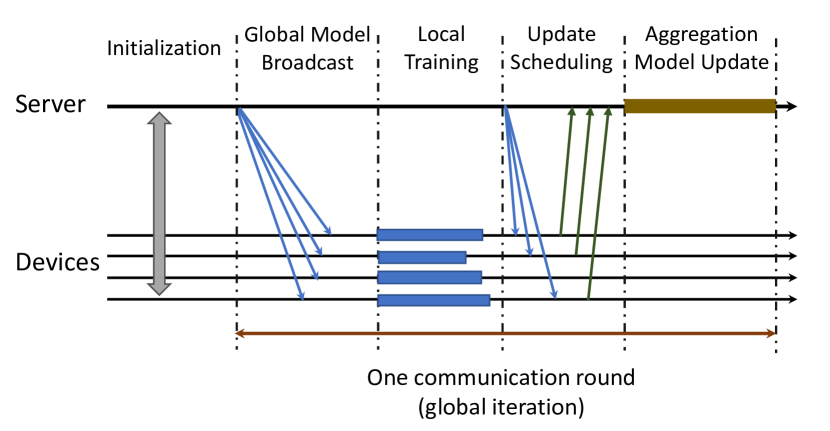
Figure 1: The FL process and information exchange between the server and the participating devices.

FedAvg is one representative FL algorithm with synchronous procedure of local training and global aggregation. The entire training process is divided into many global iterations (communication rounds), where during each iteration, the server aggregates the model updates from the participating devices computed over their locally available data. We consider a modified version of FedAvg, where an extra step of device scheduling is added after local training, as illustrated in Fig. 1. The main motivation behind this is to reduce the communication costs and delay, especially in a wireless network with limited communication resources. In the $t$-th global iteration, $t=1,2,\ldots$, the following steps are executed:

1. The server broadcasts the current global model $\boldsymbol{\theta}(t)$ to the device set $\mathcal{N}$.

2. Each device $k\in\mathcal{N}$ runs $E$ steps of stochastic gradient descent (SGD). The corresponding update rule follows

   $$\boldsymbol{\theta}_{k}(t,\tau+1)=\boldsymbol{\theta}_{k}(t,\tau)-\alpha(t,\tau)\nabla F_{k}(\boldsymbol{\theta}_{k}(t,\tau);\mathcal{B}_{k}(t,\tau)),$$

   where $\tau=0,...,E-1$ indicates the local iteration index, $\boldsymbol{\theta}_{k}(t,0)=\boldsymbol{\theta}(t)$, $\alpha(t,\tau)$ represents the learning rate and $\nabla F_{k}(\boldsymbol{\theta}_{k}(t,\tau);\mathcal{B}_{k}(t,\tau))$ denotes the gradient computed based on a randomly selected mini-batch $\mathcal{B}_{k}(t,\tau)\subseteq\mathcal{S}_{k}$. After completing the local training, each device obtains the model update as the difference between the model parameter vector before and after training, i.e.,

   $$\boldsymbol{u}_{k}(t)=\boldsymbol{\theta}_{k}(t,E)-\boldsymbol{\theta}_{k}(t,0)$$ (4)

3. After local training, a subset of devices $\Pi(t)\subseteq\mathcal{N}$ are scheduled for uploading their model updates to the server.

4. After receiving the local updates from the scheduled devices, the server aggregates the received information and updates the global model according to

   $$\boldsymbol{\theta}(t+1)=\boldsymbol{\theta}(t)+\sum_{k\in\Pi(t)}\frac{|\mathcal{S}_{k}|}{\sum_{j\in\Pi(t)}|\mathcal{S}_{j}|}\boldsymbol{u}_{k}(t).$$ (5)

This iterative procedure continues until convergence.

II-B Asynchronous FL with Periodic Aggregation

To address the straggler issue in synchronous FL without generating excessive communication load, we propose an asynchronous FL framework with periodic aggregation. The general idea is to allow asynchronous training at different devices, with the server periodically collecting updates from those devices that have completed their computation, while the rest continue their local training without being interrupted or dropped. Fig. 2 shows an example of the training and updating timeline of the original synchronous FL, fully asynchronous FL [4, 5], and our proposed scheme.

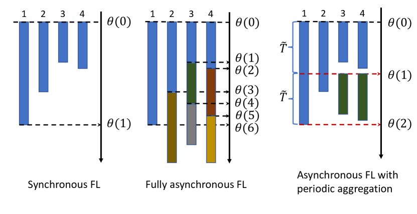
Figure 2: Conceptional difference between synchronous FL, fully asynchronous FL, and our proposed asynchronous FL with periodic aggregation. $\boldsymbol{\theta}(t)$ represents the model parameter vector in the $t$-th global iteration.

Since different devices have different computing capabilities, whenever a device finishes its local training it sends a signal to the server indicating its readiness for update reporting. At every time duration $\tilde{T}$, the server schedules a subset of ready-to-update devices. We define $\mathcal{K}(t)$ as the set of ready-to-update devices in the $t$-th global iteration. Let $\Pi(t)\subseteq\mathcal{K}(t)$ be the set of scheduled devices, with $|\Pi(t)|=\min\{R,|\mathcal{K}(t)|\}$, where $R$ is the maximal number of devices that can be scheduled. We adopt a regularization term in the loss function to alleviate potential model imbalance caused by asynchronous training. The regularized local loss at device $k$ in the $t$-th global iteration and $\tau$-th local iteration is defined by

$$H_{k}(t,\tau)=F_{k}\left(\boldsymbol{\theta}_{k}(t,\tau)\right)+\frac{\lambda}{2}\|\boldsymbol{\theta}_{k}(t,\tau)-\boldsymbol{\theta}_{k}(t,0)\|_{2}^{2},$$

where $\lambda>0$ is the regularization coefficient. For any device $k\in\Pi(t)$, its local update is thus computed as

$$\boldsymbol{\theta}_{k}(t,\tau+1)=\boldsymbol{\theta}_{k}(t,\tau)-\alpha(t,\tau)\nabla H_{k}(t,\tau),$$ (6)

with $\tau=0,...,E-1$ and $\nabla H_{k}(t,\tau)$ evaluated on a randomly selected mini-batch $\mathcal{B}_{k}(t,\tau)\subseteq\mathcal{S}_{k}$. Due to the asynchronous setup, the initial model in the first local iteration is

$$\boldsymbol{\theta}_{k}(t,0)=\boldsymbol{\theta}(s_{k}(t)),$$

where

$$s_{k}(t)=\underset{t^{\prime}<t}{\mbox{max}}\{t^{\prime}|k\in\mathcal{K}(t^{\prime})\}+1$$

indicates the latest global iteration in which device $k$ received an updated global model. After receiving the updates from all devices in $\Pi(t)$, the server conducts model aggregation as

$$\boldsymbol{\theta}(t+1)=\sum_{k\in\Pi(t)}w_{k}(t)\left[\boldsymbol{\theta}_{k}(t,0)+\boldsymbol{u}_{k}(t)\right],$$

where $\boldsymbol{u}_{k}(t)$ is defined in (4), and $w_{k}(t)$ denotes the weight coefficient, with $\sum_{k\in\Pi(t)}w_{k}(t)=1$. The updated model is then broadcast to all the devices in $\mathcal{K}(t)$ as the new global model to continue local training. Inspired by the concept of Age of Information (AoI) [26], we define the Age of Local Update (ALU) as

$$a_{k}(t)=t-s_{k}(t),$$ (7)

which represents the elapsed time since the last reception of an updated global model. The weight $w_{k}(t)$ can be related to the training data size $|\mathcal{S}_{k}|$, or the ALU $a_{k}(t)$, or combination of the both. Since the transmission of the model updates $\boldsymbol{u}_{k}(t),\forall k\in\Pi(t)$ is subject to communication resource constraints, a compressed version of $\boldsymbol{u}_{k}(t)$, denoted as $\hat{\boldsymbol{u}}_{k}(t)$, will be transmitted over the wireless channels. The compression scheme will be elaborated in the next sub-section.

II-C Physical Layer (PHY) Model

In an FL process, the communication part takes place in two phases, the server broadcasting global model to the devices (downlink transmission) and the devices reporting model updates to the server (uplink transmission). In general, the server has much higher transmit power than the devices, and the downlink transmission does not require dividing communication resources due to the broadcast channel. Therefore, we assume no compression errors in the downlink. However, uplink transmission suffers from the communication bottleneck, which makes the scheduling and resource allocation design particularly important.

We consider that at any global iteration $t$ the model updates from all devices are transmitted over a block fading channel with $n$-symbol coherence block. We assume orthogonal resource allocation among devices, i.e., $n_{k}(t)$ symbols are exclusively allocated to the device $k$ and $\sum_{k=1}^{|\Pi(t)|}n_{k}(t)=n$. Therefore, the transmissions from multiple devices are interference-free. Let $\beta_{k}$ and $h_{k}(t)$ denote the large-scale and small-scale fading of the channel from the $k$-th device to the server, respectively. Assuming that the $k$-th device has transmit power $P_{k}(t)\leq P_{k}^{\max}$ and the additive noise in the channel follows $CN(0,\sigma_{w}^{2})$, the channel capacity of the $k$-th link is

$$C_{k}(t)=\log_{2}\left(1+\frac{P_{k}(t)\beta_{k}|h_{k}(t)|^{2}}{\sigma_{w}^{2}}\right).$$ (8)

We consider that the devices apply appropriate data compression and channel coding scheme according to the channel capacity in (8) such that the transmissions of the model updates are error-free. Consequently, the server can reliably receive up to $n_{k}(t)C_{k}(t)$ bits from device $k$. The symbol allocation, $n_{k}(t),\forall k$, and data compression scheme are specified below.

II-C1 Communication resource allocation

To achieve the same level of compression loss in model updates from each device, we allocate the symbol resources in a way that

$$n_{1}(t)C_{1}(t)=...=n_{|\Pi(t)|}(t)C_{|\Pi(t)|}(t),$$ (9)

which implies that the devices with better channels are allocated with less symbols. Similar design is considered in [11].

II-C2 Sparsification and Quantization

Each device needs to compress $\boldsymbol{u}_{k}(t)$ according to the budget $n_{k}(t)C_{k}(t)$ bits. We utilize random sparsification followed by low-precision random quantization for model compression. Specifically, we define a sparsified model update $\tilde{\boldsymbol{u}}_{k}(t)\in\mathbb{R}^{d}$, where the $i$-th component $\tilde{u}_{k,i}(t),\forall i=1,...,d$ is defined by

$$\tilde{u}_{k,i}(t)=\begin{cases}u_{k,i}(t),&i\in\mathcal{V}_{k}(t)\\ 0,&\text{otherwise.}\end{cases}$$

Here, $u_{k,i}(t)$ is the $i$-th component of $\boldsymbol{u}_{k}(t)$, and $\mathcal{V}_{k}(t)$ denotes the set of reserved elements with $|\mathcal{V}_{k}(t)|=r_{k}(t)$. Then, each element $\tilde{u}_{k,i}(t),\forall i\in\mathcal{V}_{k}(t)$ is processed with $\nu$-level random quantizer $\mathcal{Q}_{\nu}:\mathbb{R}\rightarrow\mathbb{R}$ such that [27]

$$\mathcal{Q}_{\nu}(\tilde{u}_{k,i}(t))=||\tilde{\boldsymbol{u}}_{k}(t)||_{2}\cdot\text{sign}(\tilde{u}_{k,i}(t))\cdot\mathcal{Z}_{\nu}(\tilde{u}_{k,i}(t),||\tilde{\boldsymbol{u}}_{k}(t)||_{2}),$$

where

$$\mathcal{Z}_{\nu}(u,||\boldsymbol{u}||_{2})=\begin{cases}\frac{z+1}{\nu},&\text{with probability $\frac{\nu|u|}{||\boldsymbol{u}||_{2}}-z$}\\ \frac{z}{\nu},&\text{otherwise}\\ \end{cases}$$

is a random variable, $z=\lfloor\frac{\nu|u|}{||\boldsymbol{u}||_{2}}\rfloor$, and $\nu$ is the quantization level. The resulted compressed vector $\hat{\boldsymbol{u}}_{k}(t)$ has the components $\hat{u}_{k,i}(t)=\boldsymbol{1}\{i\in\mathcal{V}_{k}(t)\}\cdot\mathcal{Q}_{\nu}(\tilde{u}_{k,i}(t)),\forall i$. This random quantizer is unbiased, i.e., $\mathbb{E}[\hat{\boldsymbol{u}}_{k}(t)]=\tilde{\boldsymbol{u}}_{k}(t)$, and has quantitative bounded variance $\mathbb{E}[||\hat{\boldsymbol{u}}_{k}(t)-\tilde{\boldsymbol{u}}_{k}(t)||_{2}^{2}]\leq\frac{r_{k}(t)||\tilde{\boldsymbol{u}}_{k}(t)||_{2}^{2}}{4\nu^{2}}$. Under a fixed quantization level, we find the maximal $r_{k}(t)$ that satisfies the transmission constraint

$$\log_{2}{d\choose r_{k}(t)}+32+r_{k}(t)\left(\left\lceil\log_{2}(\nu+1)\right\rceil+1\right)\leq n_{k}(t)C_{k}(t).$$ (10)

Here, the first term $\log_{2}{d\choose r_{k}(t)}$ bits are used for sending the indexes $\mathcal{V}_{k}(t)$, the second term $32$ bits are for the vector norm value, and the third term means that $\left\lceil\log_{2}(\nu+1)\right\rceil+1$ bits are needed for transmitting each non-zero element of $\hat{\boldsymbol{u}}_{k}(t)$.

II-D Motivation of Scheduling and Aggregation Design

Under the proposed asynchronous FL setup, the key design questions are:

1. Given the communication resource constraints, how should we schedule a subset of $\mathcal{K}(t)$ for model aggregation under the scenario of heterogeneous training data distribution and wireless link quality?

2. Different devices might have different ALUs, either more recent or more outdated. How to design an appropriate weighting policy taking into account the freshness of model updates?

Recall that the goal is to minimize the global empirical loss $F(\boldsymbol{\theta})$ given in (2). We define the optimal model as $\boldsymbol{\theta}^{*}=\mbox{argmin}_{\boldsymbol{\theta}}\,F(\boldsymbol{\theta})$. Assuming $F(\boldsymbol{\theta})$ is strongly convex, implying $\nabla F\left(\boldsymbol{\theta}^{*}\right)=\boldsymbol{0}$, and $L$-smooth, i.e., for any $\boldsymbol{\theta}_{1},\boldsymbol{\theta}_{2}\in\mathbb{R}^{d}$,

$$F(\boldsymbol{\theta}_{1})-F(\boldsymbol{\theta}_{2})\leq\nabla F(\boldsymbol{\theta}_{2})^{T}(\boldsymbol{\theta}_{1}-\boldsymbol{\theta}_{2})+\frac{L}{2}||\boldsymbol{\theta}_{1}-\boldsymbol{\theta}_{2}||_{2}^{2},$$ (11)

at the $(t+1)$-th iteration we have

$$\mathbb{E}\left[F\left(\boldsymbol{\theta}\left(t+1\right)\right)\right]-F^{*}\leq\frac{L}{2}\mathbb{E}\left[||\boldsymbol{\theta}\left(t+1\right)-\boldsymbol{\theta}^{*}||_{2}^{2}\right],$$ (12)

where $\mathbb{E}\left[\cdot\right]$ denotes the expectation over all the randomness in the past iterations $1,...,t$. Note that (12) quantifies the effectiveness of model training by examining the gap between $\mathbb{E}\left[F\left(\boldsymbol{\theta}\left(t+1\right)\right)\right]$ and $F^{*}$. A smaller upper bound would potentially narrow the gap. Particularly, $\mathbb{E}\left[||\boldsymbol{\theta}\left(t+1\right)-\boldsymbol{\theta}^{*}||_{2}^{2}\right]$ in (12) can be interpreted as variance of the aggregated model produced from the model updates of the scheduled devices. We list some system factors that affect it as follows.

II-D1 Training data distribution

If all the devices have i.i.d. training data, we expect that $\Gamma\rightarrow 0$, as discussed in Sec. II. It directly follows that

$$F^{*}\rightarrow\sum_{k\in\mathcal{N}}\frac{|\mathcal{S}_{k}|}{|\mathcal{S}|}F_{k}^{*},$$

which implies a small $\mathbb{E}\left[||\boldsymbol{\theta}\left(t+1\right)-\boldsymbol{\theta}^{*}||_{2}^{2}\right]$ since $\boldsymbol{\theta}^{*}_{k}\simeq\boldsymbol{\theta}^{*}$, $\forall k\in\mathcal{N}$. However, with non-i.i.d. training data, $\boldsymbol{\theta}^{*}_{k}$ may vary a lot across different devices, which leads to a large variance of the aggregated model.

II-D2 Data compression

As the model updates are transmitted through rate-limited wireless channels, the server only receives noisy information due to data compression. Larger compression loss will give a larger variance of the aggregated model.

II-D3 Asynchronous model updates

As shown in Sec. 2, the received updates $\boldsymbol{u}_{k}(t),\forall k$ might have different ALUs, which will be an extra source of variation in $||\boldsymbol{\theta}\left(t+1\right)-\boldsymbol{\theta}^{*}||_{2}^{2}$.

From the perspective of device scheduling, we can achieve smaller $\mathbb{E}\left[||\boldsymbol{\theta}\left(t+1\right)-\boldsymbol{\theta}^{*}||_{2}^{2}\right]$ by considering the following aspects:

• The scheduled devices should construct a homogeneous representation of the entire training data set $\mathcal{S}$.

• Compression loss needs to be kept low, which motivates us to prioritize devices with better channel conditions.

From the perspective of model aggregation, we can alleviate the adverse impact of asynchronous updates by considering age-aware weighting design in the aggregation process.

III Scheduling and Aggregation Design for Asynchronous FL

We propose a scheduling policy that aims at achieving a smaller optimality gap, by considering the training data distribution and the channel conditions of ready-to-update devices. Then, the aggregation weights are adjusted accordingly to alleviate the harmful impact from asynchronous training.

III-A Channel-aware Data-importance-based Scheduling

To illustrate the idea, we consider a classification problem with labeled data. The training data set is represented by $\mathcal{S}=\{(x,y)|y\in\mathcal{L}\}$, where $\mathcal{L}=\{y_{1},...,y_{\omega}\}$ is a finite set that contains all labels and $|\mathcal{L}|=\omega$. For any device $k$, $\boldsymbol{b}_{k}=[b_{k}^{1},...,b_{k}^{\omega}]$ is defined as the label distribution in $\mathcal{S}_{k}$, where $b_{k}^{j}$ is the number of $y_{j}$-labeled samples and $\sum_{j=1}^{\omega}b_{k}^{j}=|\mathcal{S}_{k}|$. To construct a homogeneous data distribution, we may select $\Pi(t)$ to achieve the minimal label variance

$$\Omega\left(\Pi(t)\right)=\sum_{j=1}^{\omega}\Big{|}\sum_{k\in\Pi(t)}b_{k}^{j}-\bar{b}\Big{|}^{2},$$

where $\bar{b}=\frac{1}{\omega}\sum_{j=1}^{\omega}\sum_{k\in\Pi(t)}b_{k}^{j}$. Additionally, scheduling devices with better channel quality leads to smaller compression loss per device. Combine these two selection criteria, we first pick a subset $\Pi^{\prime}(t)\subseteq\mathcal{K}(t)$ comprising of devices with $\mbox{min}(0.5N,|\mathcal{K}(t)|)$ highest channel capacity $C_{k}(t)$. Next, we find $\Pi(t)=\underset{\Pi\subseteq\Pi^{\prime}(t)}{\mbox{argmin}}\,\Omega\left(\Pi\right)$.

III-B Age-aware Model Aggregation

To tackle the asynchrony in model aggregation, we assign the weights not only based on the data proportion as in (5), but also on its ALU. The age-aware weighting design follows

$$w_{k}(t)=\frac{|\mathcal{S}_{k}|{\gamma}^{a_{k}(t)}}{\sum_{i\in\Pi(t)}|\mathcal{S}_{i}|{\gamma}^{a_{i}(t)}},\forall k\in\Pi(t).$$ (13)

Here, $\gamma$ is a real-valued constant, and the choice of its value can be divided into three cases:

• $\gamma>1$, of which the system favors older local updates.

• $\gamma<1$, of which the system favors fresher local updates.

• $\gamma=1$, which is equivalent to the baseline design in (5).

Favoring older updates could potentially balance the participation frequency among the devices and reduce the risk of model training biased towards those with stronger computing capability. This design performs well when data distribution is highly non-i.i.d. and some devices with inferior computing capability possess unique training data. However, it also creates the problem of applying outdated updates on the already-evolved model. On the other hand, favoring fresher local updates would help the model to converge fast and smoothly with time, at the risk of converging to an imbalanced model biased towards devices with superior computing power. Since the proposed scheduling policy is conducted in a way that improves the homogeneity of data distribution, the advantage of “favoring fresher models” strategy becomes more convincing.

To summarize, the channel-aware data-importance-based scheduling design with favoring-fresh aggregation policy would lead to fast and smooth convergence performance. To verify the effectiveness of our design, we provide convergence analysis in Sec. IV and simulation results in V, respectively.

IV Convergence Analysis

We introduce some notations and definitions for the convergence analysis of the proposed system.

Definition 1.

(Aggregation asynchrony):

• Let $M(t)$ be the number of different versions of receive global model in the $t$-th model aggregation, i.e., the number of unique elements in the set $\{a_{k}(t)|k\in\Pi(t)\}$.

• Let $\mathcal{M}_{i}(t)\subseteq\Pi(t),i=1,...,M(t)$ be a device subset with the same ALU, i.e., $\forall k,j\in\mathcal{M}_{i}(t)$, $a_{k}(t)=a_{j}(t)$.

As in the proposed system, device scheduling is subject to the ready-to-update set $\mathcal{K}(t)$ instead of the full device set $\mathcal{N}$, we introduce the following metrics to quantify the data heterogeneity level for any device subset $\mathcal{M}$.

Definition 2.

(Data heterogeneity level): For a device subset $\mathcal{M}\subseteq\mathcal{N}$ and $\sum_{k\in\mathcal{M}}w_{k}=1$, we define

$$\Gamma_{1}(\mathcal{M})=F^{*}-\sum_{k\in\mathcal{M}}w_{k}F_{k}^{*},$$

$$\Gamma_{2}(\mathcal{M})=F\left(\boldsymbol{\theta}^{*}\right)-\sum_{k\in\mathcal{M}}w_{k}F_{k}\left(\boldsymbol{\theta}^{*}\right).$$

IV-A Assumptions

To facilitate analysis, we make the following baseline assumptions.

Assumption 1.

(Smoothness): The local loss function $F_{k}(\boldsymbol{\theta}),\forall k$ is $L$-smooth, as specified in (11), which is equivalent to Lipschitz continuous condition [28], i.e., $\forall\boldsymbol{\theta}_{1},\boldsymbol{\theta}_{2}\in\mathbb{R}^{d}$,

$$||\nabla F_{k}\left(\boldsymbol{\theta}_{1}\right)-\nabla F_{k}\left(\boldsymbol{\theta}_{2}\right)||_{2}\leq{L}||\boldsymbol{\theta}_{1}-\boldsymbol{\theta}_{2}||_{2};$$

Assumption 2.

(Strong convexity): The local loss function $F_{k}(\boldsymbol{\theta}),\forall k$ is $\mu$-strongly-convex, i.e., $\forall\boldsymbol{\theta}_{1},\boldsymbol{\theta}_{2}\in\mathbb{R}^{d}$,

$$F_{k}\left(\boldsymbol{\theta}_{1}\right)-F_{k}\left(\boldsymbol{\theta}_{2}\right)\geq\nabla F_{k}\left(\boldsymbol{\theta}_{2}\right)^{T}\left(\boldsymbol{\theta}_{1}-\boldsymbol{\theta}_{2}\right)+\frac{\mu}{2}||\boldsymbol{\theta}_{1}-\boldsymbol{\theta}_{2}||_{2}^{2};$$

followed by assumptions for stochastic gradient evaluation,

Assumption 3.

(Second moment constraint): $\forall\boldsymbol{\theta}\in\mathbb{R}^{d}$, the stochastic gradient $\nabla F_{k}(\boldsymbol{\theta};\mathcal{B}_{k}),\forall k$ satisfy

$$\mathbb{E}_{\mathcal{B}_{k}}\left[||\nabla F_{k}\left(\boldsymbol{\theta};\mathcal{B}_{k}\right)||_{2}^{2}\right]\leq C_{1}+C_{2}||\nabla F_{k}\left(\boldsymbol{\theta}\right)||_{2}^{2},$$ (14)

for some positive constant $C_{1}$ and $C_{2}$.

Note that it appears to be common in the literature to assume uniformly bounded gradient, i.e., $C_{2}=0$ in (14), and a strongly convex function over an unbounded space, e.g. [5, 6, 11, 14, 22, 24, 25, 29]. These assumptions, however, are fundamentally incompatible as there exists no strongly convex function whose gradient is uniformly bounded over $\mathbb{R}^{d}$, which is also pointed out in [30]. Working with a strongly convex function and uniformly bounded gradients requires a bounded parameter space, which yields a different (constrained) optimization problem, for which a solution algorithm would have to incorporate a projection step. We thus assume that the “noise” in the gradients is uniformly bounded (in expectation), also adopted in [28], which allows us to work with a strongly convex objective over an unbounded space.

Remark 1.

With $\tilde{T}$-periodic aggregation, the ALU of any device with training time bounded by $T_{\max}$ satisfies $0\leq a_{k}(t)\leq\lceil T_{\max}/\tilde{T}\rceil$. Then, from Definition 1 we have

$$M(t)\leq\lceil\frac{T_{\max}}{\tilde{T}}\rceil+1\triangleq M.$$ (15)

Remark 2.

Let $\mathcal{M}$ be a subset of $\mathcal{N}$. Since $\mathcal{N}$ is a finite set, there exist non-negative $\zeta_{1}$ and $\zeta_{2}$ such that

$$|\Gamma_{1}(\mathcal{M})|\leq\zeta_{1},$$ (16)

$$|\Gamma_{2}(\mathcal{M})|\leq\zeta_{2},$$ (17)

i.e., the metrics of heterogeneity level are uniformly bounded.

Additionally, for the reserved number $r_{k}(t)$, we assume that there exists a minimum $r_{\min}>0$ such that

$$\mathbb{E}[r_{k}(t)]\geq r_{\min},$$ (18)

where the expectation is with respect to the randomness in wireless channels.

IV-B Convergence Study

In the following theorem, we provide the main convergence result of our system model in a special case with one local iteration per communication round, i.e., $E=1$.

Theorem 1.

Under Assumptions 1-3, equations (15)-(18), $E=1$, diminishing learning rate $\alpha(t,0)=\frac{\beta}{t+\kappa}$ with $\beta>\frac{d}{\mu r_{\min}}>0$ and $\kappa=\mbox{max}\{\frac{dL^{2}C_{2}C_{3}\beta^{2}}{\beta\mu r_{\min}-d},4L\beta-1,1\}>0$, and partial device participation such that $\Pi(\rho)=\cup_{j=1,...,M(\rho)}\mathcal{M}_{j}(\rho)\subseteq\mathcal{N},\rho=1,...,t$, the proposed scheme satisfies

$$\mathbb{E}\left[F\left(\boldsymbol{\theta}\left(t+1\right)\right)\right]-F^{*}$$

$$\leq\frac{LM}{2\left(t+\kappa+1\right)}\left[J(\beta,\kappa)+\left(\kappa+1\right)||\boldsymbol{\theta}\left(1\right)-\boldsymbol{\theta}^{*}||_{2}^{2}\right]+\frac{LM}{2}\beta A$$

where $A=2\left(\zeta_{1}+\zeta_{2}\right)$, $C_{3}=4(1+\frac{d}{4\nu^{2}})$, and

$$J(\beta,\kappa)=\frac{\beta^{2}C_{3}(\frac{C_{1}}{2}+\frac{AL^{2}C_{2}}{\mu})+L^{2}C_{2}C_{3}\beta^{3}A}{(\frac{\mu\beta r_{\min}}{d}-1)-\frac{L^{2}C_{2}C_{3}\beta^{2}}{\kappa}}.$$

The expectation is taken over the randomness of stochastic gradient, channel gain and model compression, and device scheduling of all the past iterations.

Proof. See Section VIII-A. ∎

Remark 3.

The impact of multiple local iterations, i.e., $E>1$, on the convergence analysis has been already established and exploited in existing literature on FL (see, e.g., [29],[31, 32]). The focus of our analysis is the impact of update compression, training data heterogeneity, and intra-iteration asynchrony on the system convergence. We believe that extending our results to the case with $E>1$ is possible by following approaches from, for example, [29], [31] or [32]; this, however, would require, among other things, quantifying local model divergence. For analytical clarity and simplicity, we consider the case with $E=1$.

Remark 4.

Based on Theorem 1, the optimality gap asymptotically converges to a constant, i.e.,

$$\mathbb{E}\left[F\left(\boldsymbol{\theta}\left(t+1\right)\right)\right]-F^{*}\rightarrow\frac{LM}{2}\beta A$$

when $t\rightarrow\infty$, where $M$, $A$, and $\beta$ are defined in (15) and in the theorem. This constant can be seen as an optimality gap, which increases with $A$, $M$ and $\beta$. In an i.i.d. data scenario where $\zeta_{1}=\zeta_{2}=0$ and thus $A=0$, the system converges to the optimum even with intra-iteration asynchrony, i.e., $M>1$, and update compression, i.e., $\beta>\frac{1}{\mu}$. However, in a non-i.i.d. scenario where $A>0$, a higher level of data heterogeneity leads to a larger optimality gap. The presence of $M$ implies that intra-iteration asynchrony makes the optimality gap larger. Moreover, the presence of $\beta$ reflects that scheduling devices with better channel quality improves the performance, since a larger $r_{\min}$ allows a lower $\beta$, given $\beta>\frac{d}{\mu r_{\min}}$ specified in the theorem and $r_{\min}$ defined in (18).

Remark 5.

Apart from the asymptotic behavior, compression level of model updates also affects the per-iteration performance. With better link quality, the sparsification can be less aggressive, and/or with a higher quantization level $\nu$. As the result, the term $J(\beta,\kappa)$ can be smaller and thus the optimality gap in each iteration decreases. Moreover, as $J(\beta,\kappa)$ grows with $A$, lower data heterogeneity also improves the per-iteration performance.

These two remarks confirm the importance of considering both training data distribution and channel quality in our device scheduling design.

V Simulation Results

We perform simulations using the MNIST [33] data set for solving the hand-written digit classification problem by adopting a convolutional neural network with model dimension $d=21840$. The block fading channel spans $n$ symbols for uplink transmissions. We consider Rayleigh fading $h_{k}(t)\sim\mathcal{CN}(0,1)$ and uplink power control such that the received signal-to-noise ratio is $13$dB. The system parameters are specified as follows.

• (Training data distribution) $|\mathcal{S}|=60000$ samples are distributed evenly to all the devices. Both i.i.d. and non-i.i.d. data distribution scenarios are considered. For the i.i.d. case, $|\mathcal{S}|/N$ samples are randomly allocated to each device without replacement. For the non-i.i.d. case, the data allocation follows the setup in [2], where each device contains up to $\mbox{min}(\lfloor 200/N\rfloor,10)$ different digits.

• (Heterogeneous computing capability) We use $T_{k}$ as the local training duration of device $k$, generated from uniform distribution $T_{k}\sim\mathcal{U}(T_{\min},T_{\max})$, where $T_{\min}$ is the least possible device training time.

• (Compression) $4$-level random quantizer, $\mathcal{Q}_{4}$, is adopted.

• (Diminishing learning rate) $\alpha(1,0)=0.01$ is initially adopted, together with regularization coefficient $\lambda=0.02$.

Since the communication resources are shared by maximally $R$ devices, more scheduled devices means less communication resources per device, leading to a higher compression loss. The test accuracy results with various choices of $R$ are shown in Fig. 3. As we can see, in the i.i.d. scenario, a smaller $R$ is preferable since it gives received model updates with better precision as the result of more allocated bits per user. On the other hand, in the non-i.i.d. scenario, there exists a trade-off between compression loss and model bias, which makes the choice of $R$ important. In this work, we focus on the impact of the scheduling design for a fixed $R$. The optimal value of $R$ depends on many system parameters; its optimization could be studied in future work.

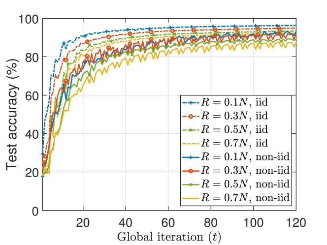
Figure 3: Test accuracy of the proposed scheme under different partial scheduling ratio, where $N=40$ and $n=50000$.

Finding the optimal value of $\tilde{T}$ analytically is highly non-trivial as we are short of a tractable expression that characterizes the relation between the optimality gap and the value of $\tilde{T}$. For the numerical results reported herein, we choose $\tilde{T}=T_{\text{max}}/4$ as this gives the best results in the simulations (see below for the comparisons between different $\tilde{T}$).

V-A Comparison of FL frameworks

First, in Fig. 4, we present the performance of our proposed design (with random scheduling and baseline aggregation, i.e., $\gamma=1$ in (13)) obtained with different values of $T_{\text{max}}/\tilde{T}$, to demonstrate the effect of the aggregation time period on the convergence performance. The performance of synchronous FedAvg is also presented for comparison. Then, in Fig. 5, we show the performance comparison between FedAvg, our proposed asynchronous FL, and FedAsync [4]. Note that to make a fair comparison between different schemes, we fix the average amount of communication resources allocated over a certain time period $T^{\prime}$. For example, if we assume there are $n$ symbols per communication round when $\tilde{T}=T_{\max}/4$ is adopted, then $4n$ symbols per round will be available for FedAvg. If FedAsync executes $N_{\text{FA}}$ iterations over time duration $T^{\prime}$, the available number of symbols per round would be $4nT^{\prime}/(T_{\max}N_{\text{FA}})$.

As shown in Fig. 4, $\tilde{T}=T_{\max}/4$ gives the best performance. However, this conclusion cannot be generalized since the result depends on many other system parameters.

The comparison between our proposed design, FedAvg, and FedAsync (with $\alpha=0.4$ and $\alpha=0.8$) is shown in Fig. 5. We observe that although FedAsync can help reduce the straggler effect, the test accuracy result shows strong fluctuation, especially with non-i.i.d. training data. For both i.i.d. and non-i.i.d. scenarios, our proposed asynchronous FL design outperforms FedAsync and FedAvg, which shows its effectiveness in eliminating the straggler effect and achieving better convergence performance.

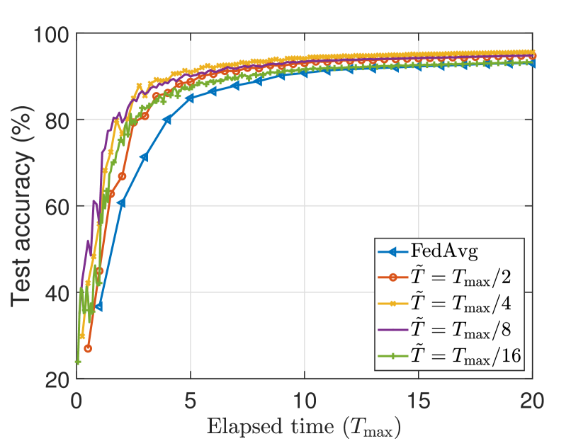
(a) i.i.d. data

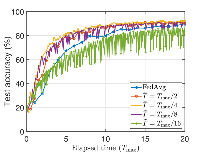
(b) non-i.i.d. data

Figure 4: Impact of $\tilde{T}$ on test accuracy of the proposed asynchronous FL with periodic aggregation in i.i.d. and non-i.i.d. scenarios, where $N=40$, $R=0.2N$ and $n=300000$.

(a) i.i.d. data

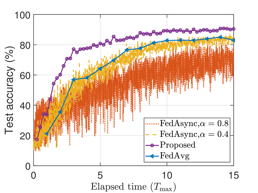
(b) non-i.i.d. data

Figure 5: Test accuracy of FedAvg, the proposed asynchronous FL with periodic aggregation, and FedAsync [4] in i.i.d. and non-i.i.d. scenarios, where $N=40$, $R=0.2N$ and $n=300000$.

V-B Validation of convergence analysis

We provide training loss comparison in Figure 6 to validate the conclusions drawn in Remarks 4 and 5. We observe the following:

• With the random and proposed scheduling methods, the training loss is lower in the i.i.d. scenario than in the non-i.i.d. scenario, which shows that a smaller $A$ leads to a lower training loss.

• For both the i.i.d. and non-i.i.d. scenarios, our proposed scheduling design outperforms random scheduling, which validates the advantage of selecting devices with better link qualities and, collectively, a more homogeneous data representation.

• To show the impact of intra-iteration asynchrony, we present the result for synchronous updates with random scheduling for i.i.d. data (the green curve). As compared to the asynchronous case (blue curve), the synchronous case has lower training loss, which shows that intra-iteration asynchrony is harmful for the convergence performance.

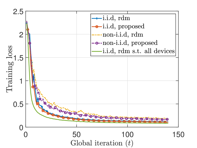
Figure 6: Training loss for random and the proposed scheduling methods in i.i.d. and non-i.i.d. scenarios, where $N=40$, $R=0.2N$ and $n=300000$.

Moreover, as shown in Fig. 4(b) with non-i.i.d. data, we see that with smaller $\tilde{T}$, which implies larger $M(t)$ and a higher feasible $\beta$, the curves for the test accuracy result are less smooth than the ones with larger $\tilde{T}$. This validates the insights in Remark 4 that in non-i.i.d. data scenarios, a higher degree of intra-iteration asynchrony and update compression leads to further degradation of the learning performance.

V-C Comparison of scheduling policies

First, the aggregation weights are set with $\gamma=1$ in (13). In Fig. 7, we show the test accuracy of the proposed scheduling design with some alternative reference methods.

• rdm: we select up to $R$ devices uniformly at random.

• BC [11]: We select up to $R$ devices with highest $C_{k}(t)$.

• BCBN2 [11]: We first find a device subset $\mathcal{C}\subseteq\mathcal{K}(t)$ with $|\mathcal{C}|$ up to $0.5N$ that has highest $C_{k}(t)$. Then, among $\mathcal{C}$ we schedule devices with up to $R$ highest $||\boldsymbol{u}_{k}(t)||_{2}^{2}$.

• Age-based [13]: We first find $\mathcal{C}$ using the same way as in BCBN2, then among $\mathcal{C}$ we schedule up to $R$ devices with highest staleness metric

  $$c_{k}(t)=\begin{cases}0,&t=0\\ \sum_{t^{\prime}=0}^{t-1}\boldsymbol{1}(k\notin\Pi(t^{\prime})),&\text{otherwise}\end{cases}$$

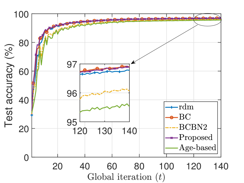
(a) i.i.d. data

(b) non-i.i.d. data

Figure 7: Test accuracy of different scheduling policies, where $N=40$, $R=0.2N$ and $n=300000$.

We see that the proposed scheduling policy outperforms the baseline random scheduling and the reference methods in both i.i.d. and non-i.i.d. scenarios. Besides, in non-i.i.d. scenario, we observe that the data-awareness in the proposed method further achieves a higher test accuracy than the pure channel-aware methods BC and BCBN2 [11].

V-D Comparison of aggregation policies

In Fig. 8, we show the performance of different aggregation policies under the proposed channel-aware data-importance-based scheduling and random scheduling methods. We see that the age-aware design outperforms the baseline with $\gamma=1$ in both i.i.d. and non-i.i.d. scenarios. For i.i.d. case, the favoring-fresh weighting strategy has an outstanding performance gain. For non-i.i.d. case, performance gain of the proposed aggregation design is more obvious when random scheduling is adopted.

(a) i.i.d. data

(b) non-i.i.d. data

Figure 8: Test accuracy of proposed aggregation policies, where $N=100$, $R=0.3N$ and $n=380000$.

VI Conclusions

In this work, we proposed an asynchronous FL framework with periodic aggregation that combines the advantages of asynchronous training and synchronous model aggregation. For the proposed design, we further developed a channel-aware data-importance-based scheduling policy and age-based aggregation design for FL under wireless resource constraints. Our proposed scheduling and aggregation design was shown to outperform existing methods, especially with heterogeneous training data among different devices. The main takeaway message is that the design principle of scheduling and resource allocation in wireless FL should be based on reducing the bias and variance of aggregated local updates. For asynchronous FL settings, balancing the freshness and usefulness of local model updates and adjusting their contributions in the new global model is also an important design aspect.

VII Acknowledgement

We thank Fredrik Jansson for his contribution to the idea of scheduling policy during his Master thesis project at the Division of Communication Systems, Linköping University.

VIII Appendix

VIII-A Proof of Theorem 1

We conduct the proof with a similar approach as in [25] and [29] except for some additional manipulations to handle the effect of asynchronous training. As briefly demonstrated in Section II-D, we begin the optimality gap analysis from (12). We define

$$c_{m}(t)=\sum_{k\in\mathcal{M}_{m}\left(t\right)}w_{k}\left(t\right)$$

as the weighting sum in $\mathcal{M}_{m}$ in $t$-th global iteration and

$$\bar{\boldsymbol{\theta}}^{\left(m\right)}\left(t+1\right)=\sum_{k\in\mathcal{M}_{m}\left(t\right)}\frac{w_{k}\left(t\right)}{c_{m}(t)}\boldsymbol{\theta}_{k}\left(t,1\right),$$

and then (12) can be rearranged as

$$\mathbb{E}\left[F\left(\boldsymbol{\theta}\left(t+1\right)\right)\right]-F^{*}\leq\frac{L}{2}\mathbb{E}\left[||\sum_{m=1}^{M\left(t\right)}c_{m}\left(t\right)\bar{\boldsymbol{\theta}}^{\left(m\right)}\left(t+1\right)-\boldsymbol{\theta}^{*}||_{2}^{2}\right]$$

$$\leq\frac{L}{2}\mathbb{E}\left[M\left(t\right)\sum_{m=1}^{M\left(t\right)}c_{m}^{2}\left(t\right)||\bar{\boldsymbol{\theta}}^{\left(m\right)}\left(t+1\right)-\boldsymbol{\theta}^{*}||_{2}^{2}\right].$$ (19)

To facilitate analysis, we first evaluate $||\bar{\boldsymbol{\theta}}^{\left(m\right)}\left(t+1\right)-\boldsymbol{\theta}^{*}||_{2}^{2}$ for any ($m$,$t$) and simplify the notation of existing variables.

• $\mathcal{M}_{m}(t)$, $\bar{\boldsymbol{\theta}}^{\left(m\right)}\left(t+1\right)$, $\bar{\boldsymbol{\theta}}^{\left(m\right)}\left(t\right)$, $w_{k}(t)$, $r_{k}(t)$, and $c_{m}(t)$ are simplified as $\mathcal{M}$, $\bar{\boldsymbol{\theta}}\left(t+1\right)$, $\bar{\boldsymbol{\theta}}\left(t\right)$, $w_{k}$, $r_{k}$, and $c$.

• Since $E=1$, for $\alpha(t,0)$ and $\mathcal{B}_{k}(t,0)$ we omit index $\tau=0$ for simplicity and rewrite them as $\alpha(t)$ and $\mathcal{B}_{k}(t)$, respectively. Moreover, $H_{k}\left(t,0\right)=F_{k}\left(\boldsymbol{\theta}_{k}(t,0)\right)$ and

  $$\nabla H_{k}\left(t,0\right)=\nabla F_{k}\left(\boldsymbol{\theta}_{k}(t,0);\mathcal{B}_{k}(t)\right).$$

• Resource allocation in (9) and transmission constraint in (10) lead to equivalent $r_{k},\forall k$. Hence, $r_{k}=r,\forall k$.

In addition, we introduce some variables and lemmas,

$$\boldsymbol{g}\left(t\right)=\sum_{k\in\mathcal{M}}\frac{w_{k}}{c}\mathcal{Q}_{\nu}\left(\nabla\tilde{F}_{k}\left(\boldsymbol{\theta}_{k}(t,0);\mathcal{B}_{k}(t)\right)\right),$$ (20)

where $-\alpha(t)\nabla\tilde{F}_{k}\left(\boldsymbol{\theta}_{k}(t,0);\mathcal{B}_{k}(t)\right)=\tilde{\boldsymbol{u}}_{k}(t)$, and

$$\bar{\boldsymbol{g}}\left(t\right)=\mathbb{E}_{\mathcal{B}_{k}(t)}\mathbb{E}_{\mathcal{Q}_{\nu}}\mathbb{E}_{\mathcal{V}_{k}(t)}\left[\boldsymbol{g}\left(t\right)\right]=\frac{r}{d}\sum_{k\in\mathcal{M}}\frac{w_{k}}{c}\nabla F_{k}\left(\boldsymbol{\theta}_{k}(t,0)\right).$$ (21)

Lemma 1.

Let $\alpha(t)\leq\frac{1}{4L}$ and $A$ defined in Theorem 1, then

$$||\bar{\boldsymbol{\theta}}\left(t\right)-\boldsymbol{\theta}^{*}-\alpha(t)\bar{\boldsymbol{g}}\left(t\right)||_{2}^{2}\leq\left(1-\frac{\mu\alpha(t)r}{d}\right)||\bar{\boldsymbol{\theta}}\left(t\right)-\boldsymbol{\theta}^{*}||_{2}^{2}+\frac{\alpha(t)rA}{d}.$$

Lemma 2.

Let $C_{3}$ and $A$ defined in Theorem 1, then the variance of $\boldsymbol{g}\left(t\right)$ fulfills

$$\mathbb{E}\left[||\boldsymbol{g}\left(t\right)-\bar{\boldsymbol{g}}\left(t\right)||_{2}^{2}\right]\leq C_{3}\mathbb{E}\left[L^{2}C_{2}||\bar{\boldsymbol{\theta}}(t)-\boldsymbol{\theta}^{*}||^{2}_{2}+\frac{C_{1}}{2}+\frac{AL^{2}C_{2}}{\mu}\right]$$

Proof. See Sections VIII-B, VIII-C.

Based on (20)-(21), $||\bar{\boldsymbol{\theta}}\left(t+1\right)-\boldsymbol{\theta}^{*}||_{2}^{2}$ can be rewritten as

$$||\bar{\boldsymbol{\theta}}\left(t+1\right)-\boldsymbol{\theta}^{*}||_{2}^{2}=||\sum_{k\in\mathcal{M}}\frac{w_{k}}{c}\boldsymbol{\theta}_{k}\left(t,0\right)-\alpha(t)\boldsymbol{g}\left(t\right)-\boldsymbol{\theta}^{*}||_{2}^{2}$$

$$=||\bar{\boldsymbol{\theta}}\left(t\right)-\alpha(t)\boldsymbol{g}\left(t\right)-\boldsymbol{\theta}^{*}-\alpha(t)\bar{\boldsymbol{g}}\left(t\right)+\alpha(t)\bar{\boldsymbol{g}}\left(t\right)||_{2}^{2}$$ (22)

$$=||\bar{\boldsymbol{\theta}}\left(t\right)-\boldsymbol{\theta}^{*}-\alpha(t)\bar{\boldsymbol{g}}\left(t\right)||_{2}^{2}+\alpha(t)^{2}||\boldsymbol{g}\left(t\right)-\bar{\boldsymbol{g}}\left(t\right)||_{2}^{2}$$

$$\quad-2\alpha(t)\left[\left(\bar{\boldsymbol{\theta}}\left(t\right)-\boldsymbol{\theta}^{*}-\alpha(t)\bar{\boldsymbol{g}}\left(t\right)\right)^{T}\left(\boldsymbol{g}\left(t\right)-\bar{\boldsymbol{g}}\left(t\right)\right)\right],$$ (23)

where (22) is due to $\boldsymbol{\theta}_{k}\left(t,0\right)=\boldsymbol{\theta}\left(t\right),\forall k$. With Lemma 1 and (18), the total expectation of (23) fulfills

$$\mathbb{E}\left[||\bar{\boldsymbol{\theta}}\left(t+1\right)-\boldsymbol{\theta}^{*}||_{2}^{2}\right]\leq\left(1-\frac{\mu\alpha(t)r_{\min}}{d}\right)\mathbb{E}\left[||\bar{\boldsymbol{\theta}}\left(t\right)-\boldsymbol{\theta}^{*}||_{2}^{2}\right]$$

$$\quad+\alpha(t)A+\alpha^{2}(t)\mathbb{E}\left[||\boldsymbol{g}\left(t\right)-\bar{\boldsymbol{g}}\left(t\right)||_{2}^{2}\right]$$

$$\quad-2\alpha(t)\mathbb{E}\left[\left(\bar{\boldsymbol{\theta}}\left(t\right)-\boldsymbol{\theta}^{*}-\alpha(t)\bar{\boldsymbol{g}}\left(t\right)\right)^{T}\left(\boldsymbol{g}\left(t\right)-\bar{\boldsymbol{g}}\left(t\right)\right)\right].$$ (24)

By definition of $\boldsymbol{g}\left(t\right)$ and $\bar{\boldsymbol{g}}(t)$, $\mathbb{E}\left[\boldsymbol{g}\left(t\right)-\bar{\boldsymbol{g}}(t)\right]=0$. Together with Lemma 2, (24) can be rearranged as

$$\mathbb{E}\left[||\bar{\boldsymbol{\theta}}\left(t+1\right)-\boldsymbol{\theta}^{*}||_{2}^{2}\right]\leq\left(1-\frac{\mu\alpha(t)r_{\min}}{d}\right)\mathbb{E}\left[||\bar{\boldsymbol{\theta}}\left(t\right)-\boldsymbol{\theta}^{*}||_{2}^{2}\right]$$

$$+\alpha(t)A+C_{3}\alpha^{2}(t)\left[L^{2}C_{2}\mathbb{E}\left[||\bar{\boldsymbol{\theta}}(t)-\boldsymbol{\theta}^{*}||^{2}_{2}\right]+\frac{C_{1}}{2}+\frac{AL^{2}C_{2}}{\mu}\right].$$

With diminishing learning rate $\alpha(t)=\frac{\beta}{t+\kappa}$, of which $\alpha(1)=\beta/(1+\kappa)\leq 1/(4L)$ satisfying the sufficient condition in Lemma 1, we claim that

$$\mathbb{E}\left[||\bar{\boldsymbol{\theta}}\left(t\right)-\boldsymbol{\theta}^{*}||_{2}^{2}\right]\leq\frac{v}{\kappa+t}+\beta A,$$ (25)

where $v=\max\left[(\kappa+1)||\boldsymbol{\theta}\left(1\right)-\boldsymbol{\theta}^{*}||_{2}^{2},C_{4}\right]$ and

$$C_{4}=\frac{\beta^{2}C_{3}(\frac{C_{1}}{2}+\frac{AL^{2}C_{2}}{\mu})+L^{2}C_{2}C_{3}\beta^{3}A}{(\frac{\mu\beta r_{\min}}{d}-1)-\frac{L^{2}C_{2}C_{3}\beta^{2}}{\kappa}}.$$

We prove (25) by induction. For $t=1$,

$$||\bar{\boldsymbol{\theta}}\left(1\right)-\boldsymbol{\theta}^{*}||_{2}^{2}=\frac{\left(\kappa+1\right)||\bar{\boldsymbol{\theta}}\left(1\right)-\boldsymbol{\theta}^{*}||_{2}^{2}}{\kappa+1}\leq\frac{v}{\kappa+1}+\beta A,$$

where $\bar{\boldsymbol{\theta}}\left(1\right)=\boldsymbol{\theta}\left(1\right)$ is the initial global model. We assume (25) holds and proceed with the case of $t+1$,

$$\mathbb{E}\left[||\bar{\boldsymbol{\theta}}\left(t+1\right)-\boldsymbol{\theta}^{*}||_{2}^{2}\right]\leq\left(1-\frac{\mu\beta r_{\min}}{\left(t+\kappa\right)d}\right)\left(\frac{v}{t+\kappa}+\beta A\right)$$

$$+\frac{\beta A}{t+\kappa}+\frac{C_{3}\beta^{2}}{\left(t+\kappa\right)^{2}}\left[L^{2}C_{2}\left(\frac{v}{t+\kappa}+\beta A\right)+\frac{C_{1}}{2}+\frac{AL^{2}C_{2}}{\mu}\right]$$

$$=\frac{t+\kappa-1}{\left(t+\kappa\right)^{2}}v+\bigg{[}\frac{[(t+\kappa)(1-\frac{\mu\beta r_{\min}}{d})+L^{2}C_{2}C_{3}\beta^{2}]v}{(t+\kappa)^{3}}$$

$$\quad+\frac{(t+\kappa)\left[\beta^{2}C_{3}\left(\frac{C_{1}}{2}+\frac{AL^{2}C_{2}}{\mu}\right)+L^{2}C_{2}C_{3}\beta^{3}A\right]}{(t+\kappa)^{3}}\bigg{]}$$

$$\quad+\frac{\beta A}{t+\kappa}+\left(1-\frac{\mu\beta r_{\min}}{\left(t+\kappa\right)d}\right)\beta A$$ (26)

$$\leq\frac{t+\kappa-1}{\left(t+\kappa\right)^{2}}v+\beta A\left[\frac{1}{t+\kappa}+1-\frac{\mu\beta r_{\min}}{\left(t+\kappa\right)d}\right]$$ (27)

$$\leq\frac{t+\kappa-1}{\left(t+\kappa\right)^{2}-1}v+\beta A=\frac{v}{t+\kappa+1}+\beta A,$$

where (27) is due to the second term in (26) being negative. Hence, (25) holds for all $t$. Recovering the indices $m$ and $t$ and plugging the result into (19),

$$\mathbb{E}\left[F\left(\boldsymbol{\theta}\left(t+1\right)\right)\right]-F^{*}$$

$$\leq\frac{L}{2}\mathbb{E}_{\mathcal{X}}\left[M\left(t\right)\sum_{m=1}^{M\left(t\right)}c_{m}^{2}\left(t\right)\left(\frac{v}{t+\kappa+1}+\beta A\right)\right]$$

$$\leq\mathbb{E}_{\mathcal{X}}\left[M\left(t\right)\right]\frac{L}{2}\left(\frac{v}{t+\kappa+1}+\beta A\right)$$

$$\leq\frac{LM}{2}\beta A+\frac{LM}{2\left(t+\kappa+1\right)}\Big{[}\left(\kappa+1\right)||\boldsymbol{\theta}\left(1\right)-\boldsymbol{\theta}^{*}||_{2}^{2}$$

$$\quad+\frac{\beta^{2}C_{3}(\frac{C_{1}}{2}+\frac{AL^{2}C_{2}}{\mu})+L^{2}C_{2}C_{3}\beta^{3}A}{(\frac{\mu\beta r_{\min}}{d}-1)-\frac{L^{2}C_{2}C_{3}\beta^{2}}{\kappa}}\Big{]},$$

where $\mathbb{E}_{\mathcal{X}}[\cdot]$ is the expectation over all the past scheduling decision, i.e., $\mathcal{X}=\{\mathcal{M}_{m}(t)|m=1,...,M(t),\forall t\}$, and $\mathbb{E}_{\mathcal{X}}\left[M\left(t\right)\right]\leq M$ because of (15).

VIII-B Proof of Lemma 1

$$||\bar{\boldsymbol{\theta}}\left(t\right)-\boldsymbol{\theta}^{*}-\alpha(t)\bar{\boldsymbol{g}}\left(t\right)||_{2}^{2}=||\bar{\boldsymbol{\theta}}\left(t\right)-\boldsymbol{\theta}^{*}||_{2}^{2}+\alpha^{2}(t)||\bar{\boldsymbol{g}}\left(t\right)||_{2}^{2}$$

$$\quad-\frac{2\alpha(t)r}{cd}\sum_{k\in\mathcal{M}}w_{k}\left(\bar{\boldsymbol{\theta}}\left(t\right)-\boldsymbol{\theta}^{*}\right)^{T}\nabla F_{k}\left(\boldsymbol{\theta}_{k}\left(t,0\right)\right)$$

$$\leq||\bar{\boldsymbol{\theta}}\left(t\right)-\boldsymbol{\theta}^{*}||_{2}^{2}+\frac{r^{2}\alpha^{2}(t)}{cd^{2}}\sum_{k\in\mathcal{M}}w_{k}||\nabla F_{k}\left(\boldsymbol{\theta}_{k}\left(t\right)\right)||_{2}^{2}$$

$$\quad-\frac{2\alpha(t)r}{cd}\sum_{k\in\mathcal{M}}w_{k}\left(\bar{\boldsymbol{\theta}}\left(t\right)-\boldsymbol{\theta}_{k}\left(t,0\right)\right)^{T}\nabla F_{k}\left(\boldsymbol{\theta}_{k}\left(t,0\right)\right)$$

$$\quad-\frac{2\alpha(t)r}{cd}\sum_{k\in\mathcal{M}}w_{k}\left(\boldsymbol{\theta}_{k}\left(t,0\right)-\boldsymbol{\theta}^{*}\right)^{T}\nabla F_{k}\left(\boldsymbol{\theta}_{k}\left(t,0\right)\right)$$ (28)

$$=||\bar{\boldsymbol{\theta}}\left(t\right)-\boldsymbol{\theta}^{*}||_{2}^{2}+\frac{r^{2}\alpha^{2}(t)}{cd^{2}}\sum_{k\in\mathcal{M}}w_{k}||\nabla F_{k}\left(\boldsymbol{\theta}_{k}\left(t\right)\right)||_{2}^{2}$$

$$\quad-\frac{2\alpha(t)r}{cd}\sum_{k\in\mathcal{M}}w_{k}\left(\boldsymbol{\theta}_{k}\left(t,0\right)-\boldsymbol{\theta}^{*}\right)^{T}\nabla F_{k}\left(\boldsymbol{\theta}_{k}\left(t,0\right)\right)$$ (29)

where (28) and (29) are due to the convexity of $||\cdot||_{2}^{2}$ and $\bar{\boldsymbol{\theta}}\left(t\right)=\boldsymbol{\theta}_{k}\left(t,0\right),\forall k$, respectively. The third term of (29) is constrained by the convexity of $F_{k}\left(\boldsymbol{\theta}\right)$,

$$-\left(\boldsymbol{\theta}_{k}\left(t,0\right)-\boldsymbol{\theta}^{*}\right)^{T}\nabla F_{k}\left(\boldsymbol{\theta}_{k}\left(t,0\right)\right)$$

$$\leq-\left(F_{k}\left(\boldsymbol{\theta}_{k}\left(t,0\right)\right)-F_{k}\left(\boldsymbol{\theta}^{*}\right)\right)-\frac{\mu}{2}||\boldsymbol{\theta}_{k}\left(t,0\right)-\boldsymbol{\theta}^{*}||_{2}^{2}.$$ (30)

By applying (30), and (38) in Section VIII-D, (29) is rearranged as

$$||\bar{\boldsymbol{\theta}}\left(t\right)-\boldsymbol{\theta}^{*}-\alpha(t)\bar{\boldsymbol{g}}\left(t\right)||_{2}^{2}$$

$$\leq||\bar{\boldsymbol{\theta}}\left(t\right)-\boldsymbol{\theta}^{*}||_{2}^{2}+\frac{r^{2}\alpha^{2}(t)}{cd^{2}}\sum_{k\in\mathcal{M}}w_{k}2L\left(F_{k}\left(\boldsymbol{\theta}_{k}\left(t,0\right)\right)-F_{k}^{*}\right)$$

$$-\frac{2\alpha(t)r}{cd}\sum_{k\in\mathcal{M}}w_{k}\Big{[}F_{k}\left(\boldsymbol{\theta}_{k}\left(t,0\right)\right)-F_{k}\left(\boldsymbol{\theta}^{*}\right)+\frac{\mu}{2}||\boldsymbol{\theta}_{k}\left(t,0\right)-\boldsymbol{\theta}^{*}||_{2}^{2}\Big{]}.$$

Based on the convexity of $||\cdot||_{2}^{2}$ and some manipulations,

$$||\bar{\boldsymbol{\theta}}\left(t\right)-\boldsymbol{\theta}^{*}-\alpha(t)\bar{\boldsymbol{g}}\left(t\right)||_{2}^{2}\leq\left(1-\frac{\mu\alpha(t)r}{d}\right)||\bar{\boldsymbol{\theta}}\left(t\right)-\boldsymbol{\theta}^{*}||_{2}^{2}$$

$$-\frac{2\alpha(t)r}{cd}\left[1-\frac{Lr\alpha(t)}{d}\right]\sum_{k\in\mathcal{M}}w_{k}\left[F_{k}\left(\boldsymbol{\theta}_{k}\left(t,0\right)\right)-F^{*}\right]$$

$$+\frac{2Lr^{2}\alpha^{2}(t)}{cd^{2}}\sum_{k\in\mathcal{M}}w_{k}\left(F^{*}-F_{k}^{*}\right)-\frac{2\alpha(t)r}{cd}\sum_{k\in\mathcal{M}}w_{k}\left(F^{*}-F_{k}\left(\boldsymbol{\theta}^{*}\right)\right).$$

Then, based on (16) and (17), we have

$$||\bar{\boldsymbol{\theta}}\left(t\right)-\boldsymbol{\theta}^{*}-\alpha(t)\bar{\boldsymbol{g}}\left(t\right)||_{2}^{2}\leq\left(1-\frac{\mu\alpha(t)r}{d}\right)||\bar{\boldsymbol{\theta}}\left(t\right)-\boldsymbol{\theta}^{*}||_{2}^{2}$$

$$-\frac{2\alpha(t)r}{cd}\left[1-\frac{Lr\alpha(t)}{d}\right]\sum_{k\in\mathcal{M}}w_{k}\left[F_{k}\left(\boldsymbol{\theta}_{k}\left(t,0\right)\right)-F^{*}\right]$$

$$+\frac{2Lr^{2}\alpha^{2}(t)}{d^{2}}\zeta_{1}+\frac{2\alpha(t)r}{d}\zeta_{2}.$$ (31)

Note that

$$\sum_{k\in\mathcal{M}}\frac{w_{k}}{c}\left(F_{k}\left(\boldsymbol{\theta}_{k}\left(t,0\right)\right)-F^{*}\right)=\sum_{k\in\mathcal{M}}\frac{w_{k}}{c}\left(F_{k}\left(\bar{\boldsymbol{\theta}}\left(t\right)\right)-F^{*}\right)$$

$$\geq\sum_{k\in\mathcal{M}}\frac{w_{k}}{c}\left(F_{k}^{*}-F^{*}\right)\geq-\zeta_{1}.$$

Since $\alpha(t)\leq 1/(4L)$, we have $-\frac{2\alpha(t)r}{d}\left[1-\frac{Lr\alpha(t)}{d}\right]<0$. Then,

$$-\frac{2\alpha(t)r}{d}\left[1-\frac{Lr\alpha(t)}{d}\right]\sum_{k\in\mathcal{M}}\frac{w_{k}}{c}\left(F_{k}\left(\boldsymbol{\theta}_{k}\left(t,0\right)\right)-F^{*}\right)$$

$$\leq\frac{2\alpha(t)r}{d}\left[1-\frac{Lr\alpha(t)}{d}\right]\zeta_{1}.$$ (32)

By plugging (32) into (31), we have

$$||\bar{\boldsymbol{\theta}}\left(t\right)-\boldsymbol{\theta}^{*}-\alpha(t)\bar{\boldsymbol{g}}\left(t\right)||_{2}^{2}\leq\left(1-\frac{\mu\alpha(t)r}{d}\right)||\bar{\boldsymbol{\theta}}\left(t\right)-\boldsymbol{\theta}^{*}||_{2}^{2}+\frac{\alpha(t)rA}{d}.$$

VIII-C Proof of Lemma 2

$$\mathbb{E}_{\mathcal{B}_{k}(t)}\mathbb{E}_{\mathcal{Q}_{\nu}}\mathbb{E}_{\mathcal{V}_{k}(t)}\left[||\boldsymbol{g}\left(t\right)-\bar{\boldsymbol{g}}\left(t\right)||_{2}^{2}\right]$$

$$=\mathbb{E}_{\mathcal{B}_{k}(t)}\mathbb{E}_{\mathcal{Q}_{\nu}}\mathbb{E}_{\mathcal{V}_{k}(t)}\Big{[}||\sum_{k\in\mathcal{M}}\frac{w_{k}}{c}\mathcal{Q}_{\nu}\left(\nabla\tilde{F}_{k}\left(\boldsymbol{\theta}_{k}(t,0);\mathcal{B}_{k}(t)\right)\right)$$

$$\quad\quad\quad\quad\quad\quad\quad\quad\quad-\frac{r}{d}\sum_{k\in\mathcal{M}}\frac{w_{k}}{c}\nabla F_{k}\left(\boldsymbol{\theta}_{k}(t,0)\right)||_{2}^{2}\Big{]}$$

$$\leq\mathbb{E}_{\mathcal{B}_{k}(t)}\mathbb{E}_{\mathcal{Q}_{\nu}}\mathbb{E}_{\mathcal{V}_{k}(t)}\Big{[}\sum_{k\in\mathcal{M}}\frac{w_{k}}{c}||\mathcal{Q}_{\nu}\left(\nabla\tilde{F}_{k}\left(\boldsymbol{\theta}_{k}(t,0);\mathcal{B}_{k}(t)\right)\right)$$

$$\quad\quad\quad\quad\quad\quad\quad\quad\quad-\frac{r}{d}\nabla F_{k}\left(\boldsymbol{\theta}_{k}(t,0)\right)||_{2}^{2}\Big{]}$$

$$=\mathbb{E}_{\mathcal{B}_{k}(t)}\mathbb{E}_{\mathcal{Q}_{\nu}}\Big{[}\sum_{k\in\mathcal{M}}\frac{w_{k}}{c}\frac{r}{d}||\mathcal{Q}_{\nu}\left(\nabla F_{k}\left(\boldsymbol{\theta}_{k}(t,0);\mathcal{B}_{k}(t)\right)\right)$$

$$\quad\quad\quad\quad\quad\quad\quad\quad\quad-\nabla F_{k}\left(\boldsymbol{\theta}_{k}(t,0)\right)||_{2}^{2}\Big{]}$$

$$\leq\frac{2r}{d}\mathbb{E}_{\mathcal{B}_{k}(t)}\mathbb{E}_{\mathcal{Q}_{\nu}}\Big{[}\sum_{k\in\mathcal{M}}\frac{w_{k}}{c}\Big{(}||\mathcal{Q}_{\nu}\left(\nabla F_{k}\left(\boldsymbol{\theta}_{k}(t,0);\mathcal{B}_{k}(t)\right)\right)$$

$$\quad-\nabla F_{k}\left(\boldsymbol{\theta}_{k}(t,0);\mathcal{B}_{k}(t)\right)||_{2}^{2}+||\nabla F_{k}\left(\boldsymbol{\theta}_{k}(t,0);\mathcal{B}_{k}(t)\right)$$

$$\quad-\nabla F_{k}\left(\boldsymbol{\theta}_{k}(t,0)\right)||_{2}^{2}\Big{)}\Big{]}$$

$$\leq\frac{2r}{d}\mathbb{E}_{\mathcal{B}_{k}(t)}\Big{[}\sum_{k\in\mathcal{M}}\frac{w_{k}}{c}\Big{(}\frac{d||\nabla F_{k}\left(\boldsymbol{\theta}_{k}(t,0);\mathcal{B}_{k}(t)\right)||_{2}^{2}}{4\nu^{2}}$$

$$\quad+||\nabla F_{k}\left(\boldsymbol{\theta}_{k}(t,0);\mathcal{B}_{k}(t)\right)-\nabla F_{k}\left(\boldsymbol{\theta}_{k}(t,0)\right)||_{2}^{2}\Big{)}\Big{]}$$

$$\leq\frac{2r}{d}(1+\frac{d}{4\nu^{2}})\left(C_{1}+C_{2}\sum_{k\in\mathcal{M}}\frac{w_{k}}{c}||\nabla F_{k}(\boldsymbol{\theta}_{k}(t,0))||_{2}^{2}\right)$$

$$\leq\frac{2r}{d}(1+\frac{d}{4\nu^{2}})\left[C_{1}+L^{2}C_{2}\sum_{k\in\mathcal{M}}\frac{w_{k}}{c}\left(||\boldsymbol{\theta}_{k}(t,0)-\boldsymbol{\theta}_{k}^{*}||^{2}_{2}\right)\right].$$ (33)

Note that

$$\sum_{k\in\mathcal{M}}\frac{w_{k}}{c}||\boldsymbol{\theta}_{k}(t,0)-\boldsymbol{\theta}_{k}^{*}||^{2}_{2}$$

$$\leq 2\sum_{k\in\mathcal{M}}\frac{w_{k}}{c}\left(||\boldsymbol{\theta}_{k}(t,0)-\boldsymbol{\theta}^{*}||^{2}_{2}+||\boldsymbol{\theta}^{*}-\boldsymbol{\theta}_{k}^{*}||^{2}_{2}\right)$$

$$\leq 2\sum_{k\in\mathcal{M}}\frac{w_{k}}{c}\left[||\boldsymbol{\theta}_{k}(t,0)-\boldsymbol{\theta}^{*}||^{2}_{2}+\frac{2}{\mu}\left(F_{k}\left(\boldsymbol{\theta}^{*}\right)-F_{k}\left(\boldsymbol{\theta}_{k}^{*}\right)\right)\right]$$

$$\leq 2||\bar{\boldsymbol{\theta}}(t)-\boldsymbol{\theta}^{*}||^{2}_{2}+\frac{2}{\mu}A.$$ (34)

Plugging (34) into (33), we have

$$\mathbb{E}_{\mathcal{B}_{k}(t)}\mathbb{E}_{\mathcal{Q}_{\nu}}\mathbb{E}_{\mathcal{V}_{k}(t)}\left[||\boldsymbol{g}\left(t\right)-\bar{\boldsymbol{g}}\left(t\right)||_{2}^{2}\right]$$

$$\leq\frac{2r}{d}(1+\frac{d}{4\nu^{2}})\left[C_{1}+2L^{2}C_{2}\left(||\bar{\boldsymbol{\theta}}(t)-\boldsymbol{\theta}^{*}||^{2}_{2}+\frac{A}{\mu}\right)\right]$$

$$\leq C_{3}L^{2}C_{2}||\bar{\boldsymbol{\theta}}(t)-\boldsymbol{\theta}^{*}||^{2}_{2}+C_{3}\left(\frac{C_{1}}{2}+\frac{AL^{2}C_{2}}{\mu}\right).$$ (35)

As the bound in (35) does not depend on current scheduling policy $\mathcal{M}$, the proof is completed.

VIII-D Proof of $2L\left[F_{k}\left(\boldsymbol{\theta}\right)-F_{k}^{*}\right]\geq||\nabla F_{k}\left(\boldsymbol{\theta}\right)||_{2}^{2}$

Let $\boldsymbol{\theta}_{1},\boldsymbol{\theta}_{2}\in\mathbb{R}^{d}$. Since $F_{k}\left(\boldsymbol{\theta}\right)$ is $L$-smooth,

$$F_{k}\left(\boldsymbol{\theta}_{1}\right)\leq F_{k}\left(\boldsymbol{\theta}_{2}\right)+\nabla F_{k}\left(\boldsymbol{\theta}_{2}\right)^{T}\left(\boldsymbol{\theta}_{1}-\boldsymbol{\theta}_{2}\right)+\frac{L}{2}||\boldsymbol{\theta}_{1}-\boldsymbol{\theta}_{2}||_{2}^{2}.$$ (36)

Define the right-hand side of (36) as a new function

$$g\left(\boldsymbol{\theta}_{1}\right)=F_{k}\left(\boldsymbol{\theta}_{2}\right)+\nabla F_{k}\left(\boldsymbol{\theta}_{2}\right)^{T}\left(\boldsymbol{\theta}_{1}-\boldsymbol{\theta}_{2}\right)+\frac{L}{2}||\boldsymbol{\theta}_{1}-\boldsymbol{\theta}_{2}||_{2}^{2}.$$

Since $g\left(\boldsymbol{\theta}_{1}\right)$ is a quadratic function with global minimum $g\left(\boldsymbol{\theta}^{*}\right)$ and $\nabla g\left(\boldsymbol{\theta}^{*}\right)=\boldsymbol{0}$, it follows that

$$\nabla F_{k}\left(\boldsymbol{\theta}_{2}\right)+L\left(\boldsymbol{\theta}^{*}-\boldsymbol{\theta}_{2}\right)=\boldsymbol{0}\text{, and }\boldsymbol{\theta}^{*}=\frac{-\nabla F_{k}\left(\boldsymbol{\theta}_{2}\right)}{L}+\boldsymbol{\theta}_{2}.$$

Then, the global minimum is

$$g\left(\boldsymbol{\theta}^{*}\right)=F_{k}\left(\boldsymbol{\theta}_{2}\right)-\frac{1}{2L}||\nabla F_{k}\left(\boldsymbol{\theta}_{2}\right)||_{2}^{2}.$$ (37)

Combining (37) and (36),

$$\mbox{min}_{\boldsymbol{\theta}}F_{k}\left(\boldsymbol{\theta}\right)\leq F_{k}\left(\boldsymbol{\theta}_{2}\right)-\frac{1}{2L}||\nabla F_{k}\left(\boldsymbol{\theta}_{2}\right)||_{2}^{2}$$

and hence

$$2L\left[F_{k}\left(\boldsymbol{\theta}_{2}\right)-F_{k}^{*}\right]\geq||\nabla F_{k}\left(\boldsymbol{\theta}_{2}\right)||_{2}^{2}.$$ (38)

Chung-Hsuan Hu received the B.Sc. degree in electronics and electrical engineering, and M.Sc. degree in communications engineering from National Yang Ming Chiao Tung University (NYCU), Taiwan, in 2010 and 2012, respectively. From 2013 to 2020, she worked as a communication systems engineer with MediaTek Inc., Taiwan. Currently, she is pursuing the Ph.D. degree with the Division of Communication Systems, Department of Electrical Engineering, Linköping University, Sweden. Her research interests include distributed learning systems and wireless communications.

Zheng Chen (Member, IEEE) is an Assistant Professor with the Department of Electrical Engineering, Linköping University, Sweden. She received the B.Sc. degree from Huazhong University of Science and Technology (HUST), China, in 2011. Then, she received the M.Sc. and Ph.D. degrees from CentraleSupélec, Université Paris-Saclay, France, in 2013 and 2016, respectively. Since January 2017, she has been with Linköping University, Sweden. Her main research interests include wireless communications, distributed intelligent systems, and complex networks. She was the recipient of the 2020 IEEE Communications Society Young Author Best Paper Award. She was selected as an Exemplary Reviewer for IEEE Communications Letters in 2016, for IEEE Transactions on Wireless Communications in 2017, and for IEEE Transactions on Communications in 2019. She served as the workshop co-chair of the IEEE GLOBECOM Workshop on Wireless Communications for Distributed Intelligence in 2021 and 2022. She is currently an Editor at IEEE Transactions on Green Communications and Networking.

Erik G. Larsson (Fellow, IEEE) received the Ph.D. degree from Uppsala University, Uppsala, Sweden, in 2002. He is currently Professor of Communication Systems at Linköping University (LiU) in Linköping, Sweden. He was with the KTH Royal Institute of Technology in Stockholm, Sweden, the George Washington University, USA, the University of Florida, USA, and Ericsson Research, Sweden. His main professional interests are within the areas of wireless communications and signal processing. He co-authored Space-Time Block Coding for Wireless Communications (Cambridge University Press, 2003) and Fundamentals of Massive MIMO (Cambridge University Press, 2016). He served as chair of the IEEE Signal Processing Society SPCOM technical committee (2015–2016), chair of the IEEE Wireless Communications Letters steering committee (2014–2015), member of the IEEE Transactions on Wireless Communications steering committee (2019-2022), General and Technical Chair of the Asilomar SSC conference (2015, 2012), technical co-chair of the IEEE Communication Theory Workshop (2019), and member of the IEEE Signal Processing Society Awards Board (2017–2019). He was Associate Editor for, among others, the IEEE Transactions on Communications (2010-2014), the IEEE Transactions on Signal Processing (2006-2010), and the IEEE Signal Processing Magazine (2018-2022). He received the IEEE Signal Processing Magazine Best Column Award twice, in 2012 and 2014, the IEEE ComSoc Stephen O. Rice Prize in Communications Theory in 2015, the IEEE ComSoc Leonard G. Abraham Prize in 2017, the IEEE ComSoc Best Tutorial Paper Award in 2018, and the IEEE ComSoc Fred W. Ellersick Prize in 2019.

References

• [1] J. Konečnỳ, H. B. McMahan, D. Ramage, and P. Richtárik, “Federated optimization: Distributed machine learning for on-device intelligence,” arXiv preprint arXiv:1610.02527, 2016.
• [2] B. McMahan, E. Moore, D. Ramage, S. Hampson, and B. A. y Arcas, “Communication-efficient learning of deep networks from decentralized data,” in Artificial Intelligence and Statistics, 2017, pp. 1273–1282.
• [3] J. Chen, R. Monga, S. Bengio, and R. Jozefowicz, “Revisiting distributed synchronous SGD,” in International Conference on Learning Representations Workshop Track, 2016.
• [4] C. Xie, S. Koyejo, and I. Gupta, “Asynchronous federated optimization,” in NeurIPS workshop on Optimization for Machine Learning, 2020.
• [5] Y. Chen, Y. Ning, M. Slawski, and H. Rangwala, “Asynchronous online federated learning for edge devices with non-IID data,” in IEEE International Conference on Big Data, 2020, pp. 15–24.
• [6] Z. Wang, H. Xu, J. Liu, H. Huang, C. Qiao, and Y. Zhao, “Resource-efficient federated learning with hierarchical aggregation in edge computing,” in IEEE INFOCOM, 2021, pp. 1–10.
• [7] J. Nguyen, K. Malik, H. Zhan, A. Yousefpour, M. Rabbat, M. Malek, and D. Huba, “Federated learning with buffered asynchronous aggregation,” in Proceedings of The 25th International Conference on Artificial Intelligence and Statistics, vol. 151, 2022, pp. 3581–3607.
• [8] C. Zhou, H. Tian, H. Zhang, J. Zhang, M. Dong, and J. Jia, “Tea-fed: Time-efficient asynchronous federated learning for edge computing,” in Proceedings of the 18th ACM International Conference on Computing Frontiers, 2021, p. 30–37.
• [9] T. Gafni, N. Shlezinger, K. Cohen, Y. C. Eldar, and H. V. Poor, “Federated learning: A signal processing perspective,” IEEE Signal Processing Magazine, vol. 39, no. 3, pp. 14–41, 2022.
• [10] H. H. Yang, Z. Liu, T. Q. S. Quek, and H. V. Poor, “Scheduling policies for federated learning in wireless networks,” IEEE Trans. on Communications, vol. 68, no. 1, pp. 317–333, 2020.
• [11] M. M. Amiri, D. Gündüz, S. R. Kulkarni, and H. Vincent Poor, “Convergence of update aware device scheduling for federated learning at the wireless edge,” IEEE Trans. on Wireless Communications, pp. 1–1, 2021.
• [12] B. Luo, W. Xiao, S. Wang, J. Huang, and L. Tassiulas, “Tackling system and statistical heterogeneity for federated learning with adaptive client sampling,” in IEEE INFOCOM, 2022, pp. 1739–1748.
• [13] H. H. Yang, A. Arafa, T. Q. Quek, and H. V. Poor, “Age-based scheduling policy for federated learning in mobile edge networks,” in IEEE International Conference on Acoustics, Speech and Signal Processing (ICASSP), 2020, pp. 8743–8747.
• [14] M. Salehi and E. Hossain, “Federated learning in unreliable and resource-constrained cellular wireless networks,” IEEE Trans. on Communications, vol. 69, no. 8, pp. 5136–5151, 2021.
• [15] D. Liu, G. Zhu, J. Zhang, and K. Huang, “Data-importance aware user scheduling for communication-efficient edge machine learning,” IEEE Trans. on Cognitive Communications and Networking, pp. 1–1, 2020.
• [16] M. E. Ozfatura, J. Zhao, and D. Gündüz, “Fast federated edge learning with overlapped communication and computation and channel-aware fair client scheduling,” in IEEE 22nd International Workshop on Signal Processing Advances in Wireless Communications (SPAWC), 2021, pp. 311–315.
• [17] H. Chen, S. Huang, D. Zhang, M. Xiao, M. Skoglund, and H. V. Poor, “Federated learning over wireless IoT networks with optimized communication and resources,” IEEE Internet of Things Journal, pp. 1–1, 2022.
• [18] A. Taïk, H. Moudoud, and S. Cherkaoui, “Data-quality based scheduling for federated edge learning,” in IEEE 46th Conference on Local Computer Networks (LCN), 2021, pp. 17–23.
• [19] G. Shen, D. Gao, L. Yang, F. Zhou, D. Song, W. Lou, and S. Pan, “Variance-reduced heterogeneous federated learning via stratified client selection,” 2022. [Online]. Available: https://arxiv.org/abs/2201.05762
• [20] W. Shi, S. Zhou, Z. Niu, M. Jiang, and L. Geng, “Joint device scheduling and resource allocation for latency constrained wireless federated learning,” IEEE Trans. on Wireless Communications, vol. 20, no. 1, pp. 453–467, 2021.
• [21] M. M. Wadu, S. Samarakoon, and M. Bennis, “Joint client scheduling and resource allocation under channel uncertainty in federated learning,” IEEE Trans. on Communications, vol. 69, no. 9, pp. 5962–5974, 2021.
• [22] M. Chen, Z. Yang, W. Saad, C. Yin, H. V. Poor, and S. Cui, “A joint learning and communications framework for federated learning over wireless networks,” IEEE Trans. on Wireless Communications, vol. 20, no. 1, pp. 269–283, 2021.
• [23] H.-S. Lee and J.-W. Lee, “Adaptive transmission scheduling in wireless networks for asynchronous federated learning,” IEEE Journal on Selected Areas in Communications, vol. 39, no. 12, pp. 3673–3687, 2021.
• [24] Z. Chai, Y. Chen, A. Anwar, L. Zhao, Y. Cheng, and H. Rangwala, “FedAT: A high-performance and communication-efficient federated learning system with asynchronous tiers,” in Proceedings of the International Conference for High Performance Computing, Networking, Storage and Analysis, 2021.
• [25] X. Li, K. Huang, W. Yang, S. Wang, and Z. Zhang, “On the convergence of FedAvg on non-IID data,” in International Conference on Learning Representations, 2020.
• [26] A. Kosta, N. Pappas, and V. Angelakis, “Age of information: A new concept, metric, and tool,” Foundations and Trends in Networking, vol. 12, no. 3, pp. 162–259, 2017.
• [27] D. Alistarh, D. Grubic, J. Li, R. Tomioka, and M. Vojnovic, “QSGD: Communication-efficient SGD via gradient quantization and encoding,” in Proceedings of the 31st International Conference on Neural Information Processing Systems, 2017, pp. 1707–1718.
• [28] L. Bottou, F. E. Curtis, and J. Nocedal, “Optimization methods for large-scale machine learning,” SIAM Review, vol. 60, no. 2, pp. 223–311, 2018. [Online]. Available: https://doi.org/10.1137/16M1080173
• [29] S. U. Stich, “Local SGD converges fast and communicates little,” in International Conference on Learning Representations, 2019. [Online]. Available: https://openreview.net/forum?id=S1g2JnRcFX
• [30] L. M. Nguyen, P. H. Nguyen, P. Richtárik, K. Scheinberg, M. Takáč, and M. van Dijk, “New convergence aspects of stochastic gradient algorithms,” Journal of Machine Learning Research, vol. 20, no. 176, pp. 1–49, 2019. [Online]. Available: http://jmlr.org/papers/v20/18-759.html
• [31] N. Singh, D. Data, J. George, and S. Diggavi, “SQuARM-SGD: Communication-efficient momentum sgd for decentralized optimization,” IEEE Journal on Selected Areas in Information Theory, vol. 2, no. 3, pp. 954–969, 2021.
• [32] A. Koloskova, N. Loizou, S. Boreiri, M. Jaggi, and S. Stich, “A unified theory of decentralized SGD with changing topology and local updates,” in Proceedings of the 37th International Conference on Machine Learning, vol. 119.   PMLR, 13–18 Jul 2020, pp. 5381–5393.
• [33] Y. LeCun and C. Cortes, “MNIST handwritten digit database,” 2010. [Online]. Available: http://yann.lecun.com/exdb/mnist/