Smoothing volatility targeting

Abstract

We propose an alternative approach towards cost mitigation in volatility-managed portfolios based on smoothing the predictive density of an otherwise standard stochastic volatility model. Specifically, we develop a novel variational Bayes estimation method that flexibly encompasses different smoothness assumptions irrespective of the persistence of the underlying latent state. Using a large set of equity trading strategies, we show that smoothing volatility targeting helps to regularise the extreme leverage/turnover that results from commonly used realised variance estimates. This has important implications for both the risk-adjusted returns and the mean-variance efficiency of volatility-managed portfolios, once transaction costs are factored in. An extensive simulation study shows that our variational inference scheme compares favourably against existing state-of-the-art Bayesian estimation methods for stochastic volatility models.

Keywords: Volatility targeting, mean-variance efficiency, Bayesian methods, stochastic volatility models, variational Bayes inference.

JEL codes: G11, G12, G17, C23

1 Introduction

The widespread evidence that volatility tends to cluster over time and negatively correlates with realised returns have motivated the use of volatility targeting to dynamically adjust the notional exposure to a given portfolio. A conventional approach to volatility targeting builds upon the idea that the capital exposure to a given portfolio is levered up (scaled down) based on the inverse of the previous month’s realised variance. The theoretical foundation lies in the evolution of the risk-return trade-off over time (see, e.g., Moreira and Muir, 2017). However, volatility management based on realised variance estimates is associated with a dramatic increase in portfolio turnover and significant time-varying leverage. This casts doubt on the usefulness of conventional volatility-managed portfolios, especially for large institutional investors with high all-in implementation costs (see, e.g., Patton and Weller, 2020).

Figure 1 shows this case in point. The left panel shows the volatility-managed portfolio allocation based on realised variance estimates for three common portfolios; the market, and the size and momentum factors as originally proposed by Fama and French (1996) and Jegadeesh and Titman (1993), respectively. Simple volatility targeting leads to a tenfold notional exposure compared to the original equity strategy. This excess leverage is pervasive across a broad set of 158 equity trading strategies which will be introduced in Section 3. For instance, the middle panel in Figure 1 shows that volatility targeting based on realised variance leads to a leverage between 1.8 and 4 times for more than 10%, and between 3 to 11 times for at least 1% of the original 158 equity strategies. This makes volatility-managed strategies potentially both risky and costly to implement, especially when volatility targeting is missed and/or forecasts are not sufficiently accurate (see, e.g., Bongaerts et al., 2020).

A simple approach towards cost mitigation is to reduce liquidity demand by slowing down the time-series variation in the factor leverage; this is often achieved by using less erratic estimates of risk, such as the realised volatility instead of the realised variance, or by introducing leverage constraints in the form of a capped notional exposure (see, e.g., Moreira and Muir, 2017, Cederburg et al., 2020, Barroso and Detzel, 2021). While imposing leverage constraints may simplifies an empirical analysis, they do not regularise the often erratic monthly underlying volatility estimates and are typically set arbitrarily, absent sounded economic arguments for their optimal setup. In this respect, the economic value of leverage constraints is an indirect function of the statistical accuracy of the underlying volatility estimates.

In this paper, we propose an alternative approach towards slowing down liquidity demand in volatility-managed portfolios which is based on smoothing the predictive density of an otherwise standard stochastic volatility model. Our view is that by smoothing monthly volatility forecasts, one can regularise trading turnover and therefore mitigate the effect of transaction costs on volatility-managed portfolios. Such regularisation is achieve by a variational Bayes inference scheme which flexibly encompasses different smoothness assumptions irrespective of the underlying persistence of the latent state. Put it differently, our underlying assumption is that actual monthly returns’ volatility may simply follow a conventional autoregressive latent stochastic process. However, monthly volatility forecasts can be noisy, which leads to extreme portfolio turnover from volatility targeting. As a result, one could “filter out” the noise based on a posterior approximation density which embeds both non-smooth predictive densities and different types of smoothing, e.g., wavelet basis functions (see Rue and Held, 2005).

We evaluate the economic performance of our smooth volatility prediction based on a broad sample of 158 equity trading strategies. We first consider the nine equity factors examined by Moreira and Muir (2017). We augment the first group of test portfolios with a second group covering a broader set of trading strategies based on the list of 153 characteristic-managed portfolios, or “factors”, reported in Jensen et al. (2022). In addition to previous month’s realised variance (henceforth RV), we benchmark our smooth volatility-managed portfolios (SSV) against several alternative implementations of volatility-targeting. The first uses the expected variance from a simple AR(1) rather than realized variance (RV AR), which helps to reduce the extremity of the weights. Second, we consider an alternative six-month window to estimate the longer-term realised variance (RV6) as proposed by Barroso and Santa-Clara (2015), Barroso and Detzel (2021). Third, we consider both a long-memory model for volatility forecast as proposed by Corsi (2009) (HAR), and a standard AR(1) stochastic volatility model (SV) (see, e.g., Taylor, 1994). Finally, we consider a plain GARCH(1,1) specification (Garch), which has been proved a challenging benchmark in volatility forecasting (see, Hansen and Lunde, 2005).

1.1 Main findings

Our empirical tests evaluate the performance of alternative volatility-managed implementations of a broad set of volatility managed portfolios, each of them constructed as

$$y^{\sigma}_{t} =\frac{c^{*}}{\widehat{\sigma}_{t-1|t}^{2}}y_{t},$$ (1)

where $y^{\sigma}_{t}$ and $y_{t}$ are the scaled and the original portfolio’s excess returns in month $t$, respectively. Here $\widehat{\sigma}_{t-1|t}^{2}$ is the variance forecast of the original portfolio’s returns at month $t$ based on information available up to month $t-1$. We follow Cederburg et al. (2020) and consider both an unconditional and a real-time implementation of volatility targeting. The former implies that the constant $c^{*}$ is chosen such that the unconditional variance of the managed $y^{\sigma}_{t}$ and unmanaged $y_{t}$ portfolios coincide. For the real-time implementation, $c_{t}^{*}$ is time-varying and is chosen such that the variance of the managed and unmanaged portfolios coincide only conditional on the returns up to month $t$.

Most prior studies assess the value of volatility targeting strategies by comparing the Sharpe ratios obtained by scaled factors $y_{t}^{\sigma}$ as in Eq.(1), with the Sharpe ratios obtained from the original factors $y_{t}$ (see, e.g., Barroso and Santa-Clara, 2015, Daniel and Moskowitz, 2016, Moreira and Muir, 2017, Bianchi et al., 2022). We follow this approach and confirm the existing evidence in the literature that stand-alone investments in volatility-managed portfolios do not systematically improve upon unmanaged factors (see, e.g., Cederburg et al., 2020, Barroso and Detzel, 2021). However, volatility targeting based on our smooth volatility forecasts substantially improves both upon conventional realised variance measures and a variety of competing volatility forecasting methods. Specifically, volatility-managed portfolios show a substantially lower turnover compared to alternative volatility forecasting methods. The right panel of Figure 1 shows this case in point. The time variation of leverage for the volatility-managed market portfolio is much lower for our SSV compared to a standard RV or a lower-frequency RV6.

Perhaps more importantly, we show that greater portfolio stability translates into a substantially large risk-adjusted performance. For conservative levels of transaction costs, our SSV produces a substantially higher economic utility compared to both standard and non-standard volatility forecasting methods. For each equity strategy and volatility-targeting methodology, we estimate the spanning regression on both the scaled and unscaled returns,

$$y^{\sigma}_{t} =\alpha+\beta y_{t}+\epsilon_{t},$$ (2)

The economic implication of $\alpha>0$ is that volatility scaled portfolios may expand the mean-variance frontier relative to the unscaled portfolios (see, e.g., Gibbons et al., 1989). We test this assumption by comparing the certainty equivalent return (CER) when factoring in moderate levels of notional transaction costs, with and without leverage constraints. Specifically, we compare two strategies: (i) a strategy that allocates between a given volatility-managed portfolio and its corresponding original portfolio, and (ii) a strategy constrained to invest only in the original portfolio. The baseline combination correspond to the optimal mean-variance allocation assuming a risk aversion coefficient equal to five. We show that when transaction costs are considered, our SSV stands out as the most profitable rescaling method, on average. Perhaps more interestingly, the SSV is the only with a positive median CER differential with respect to the unmanaged portfolio strategies. That is, the economic gain is positive for at least 50% of the equity strategies considered. Interestingly, a regularisation of the volatility targeting weights based on leverage constraints does not reduce the gap between our SSV method and all the alternative weighting schemes we consider. Similarly, the economic gain from a mean-variance combination strategy of the unmanaged and managed portfolios is substantially in favour of our SSV method.

In addition to the empirical analysis on a broad set of equity trading strategies, we explore the statistical underpinnings of our modeling framework through an extensive simulation exercise. We compare the estimation accuracy of our VB inference scheme against state-of-the-art Bayesian methods, such as MCMC (see, e.g., Hosszejni and Kastner, 2021) and variational Bayes (see, e.g., Chan and Yu, 2022). The results show that when we do not arbitrarily impose any smoothness in the posterior estimates of the latent stochastic volatility state, our algorithm is as accurate as MCMC and existing variational Bayes methods. Yet, when we smooth the posterior estimates the accuracy deteriorates. This is expected since the wavelet basis functions mechanically tilts the posterior estimates of the parameters towards a more persistent latent state relative to the actual data generating process.

1.2 Reference literature

In addition to Moreira and Muir (2017), our work contributes to a growing literature that seeks to understand the origins and the dynamic properties of volatility-managed portfolios (see, e.g., Harvey et al., 2018, Bongaerts et al., 2020, Cederburg et al., 2020, Liu et al., 2019, Barroso and Detzel, 2021, Wang and Yan, 2021, among others). Liu et al. (2019) shows that a real-time implementation of volatility targeting suffers from severe drawdowns, compared to unmanaged portfolios. Similarly, Cederburg et al. (2020) shows that volatility-managed portfolios do not systematically outperform the corresponding unmanaged equity strategies.

We contribute to this literature by highlighting the importance of volatility modeling for the profitability of volatility-managed portfolios. Specifically, we show that smoothing the volatility forecasts provide an intuitive regularization to volatility targeting. This translates in an economically better performance versus realised variance measures when notional trading costs are factored in. In addition, we explicitly acknowledge that the uncertainty around the volatility predictions might be pervasive. By taking a Bayesian approach we can quantify the uncertainty around the scaled portfolio returns, so that a more direct statistical comparison between scaled and unscaled factors can be made.

A second strand of literature we contribute to, relates to the estimation of stochastic volatility models. The non-linear interaction between the latent volatility state and the observed returns lead to a likelihood function that depends upon high dimensional integrals. A variety of estimation procedures have been proposed to overcome this difficulty, including the generalized method of moments (GMM) of Melino and Turnbull (1990), the quasi maximum likelihood (QML) approach of Harvey et al. (1994) and Ruiz (1994), and the efficient method of moments (EMM) of Gallant et al. (1997). Within the context of Bayesian methods, the analysis of stochastic volatility models has been initially proposed by Kim et al. (1998), Durbin and Koopman (2000), Jacquier et al. (2002, 2004), Shephard and Pitt (2004), Durbin and Koopman (2000). We contribute to this literature by proposing a novel variational Bayes estimation framework which allows to flexibly smooth the predictive density of the latent stochastic volatility state, irrespective of the underlying assumption about the data generating process. Our approach is general, meaning that encompasses different smoothness assumptions for the volatility forecasts without changing the underlying model structure.

Finally, this paper connects to a third strand of literature that introduces the use of variational Bayes methods for economic forecasting (see, e.g., Gefang et al., 2019, Koop and Korobilis, 2020, Chan and Yu, 2022). Variational approximate methods (Bishop, 2006) have become popular as computational feasible alternatives to Markov Chain Monte Carlo (MCMC) for approximating the posterior distributions. This type of inferential methods have been used in a wide range of applications, ranging from statistics (Rustagi, 1976) to quantum mechanics (Sakurai, 1994), statistical mechanics (Parisi, 1988), machine learning (Hinton and Van Camp, 1993) and then generalized to many probabilistic models, taking advantage of the graphical models’ representation (Jordan et al., 1999). We contribute to this literature by proposing a flexible approximation based on a Gaussian Markov random field approximation of the latent stochastic volatility state. This allows to consider both non-smooth and smooth volatility forecasts based on a simple twist in the posterior approximating density of the latent state.

2 Modeling framework

Let consider a standard univariate dynamic model with stochastic volatility (Taylor, 1994). A general specification is based on a state-space representation of the form:

$$y_{t} =\mathbf{x}_{t}^{\intercal}\beta+\exp(h_{t}/2)\varepsilon_{t}, \varepsilon_{t}\sim\mathsf{N}(0,1)$$ (3)

$$h_{t} =c+\rho(h_{t-1}-c)+u_{t}, u_{t}\sim\mathsf{N}(0,\eta^{2}),$$ (4)

where $y_{t}$, $\mathbf{x}_{t}\in\mathbb{R}^{p}$, $h_{t}=\log\sigma_{t}^{2}$ are, respectively, the log-return, a set of covariates, and the log-volatility of an equity strategy at time $t$, for $t=1,2,\dots,n$. The error terms $\varepsilon_{t}$ and $u_{t}$ are mutually independent Gaussian white noise processes. The latent process in (4) is a conventional autoregressive process of order one, with unconditional mean $c$, persistence $\rho$, and conditional variance $\eta^{2}$. We assume $|\rho|<1$, so that the initial state $h_{0}$ can be sampled from the marginal distribution, i.e. $h_{0}\sim\mathsf{N}\left(c,\frac{\eta^{2}}{1-\rho^{2}}\right)$. Notice that, for comparability with the existing literature on volatility-managed portfolios, we assume a constant mean $\mu$ in the observation equation (3), such that there are no covariates and $\mu=\mathbf{x}_{t}^{\intercal}\beta$ with $\mathbf{x}_{t}$ an n-dimensional vector of ones. However, in the following, we provide the full specification of our variational Bayes inference scheme under the general model with covariates.

2.1 Variational Bayes inference

A variational Bayes approach to inference requires to minimize the Kullback-Leibler ($\mathit{KL}$) divergence between an approximating density $q(\boldsymbol{\vartheta})$ and the true posterior density $p(\boldsymbol{\vartheta}|\mathbf{y})$, (see, e.g. Blei et al., 2017). The $\mathit{KL}$ divergence cannot be directly minimized with respect to $\boldsymbol{\vartheta}$ because it involves the expectation with respect to the unknown true posterior distribution. Ormerod and Wand (2010) show that the problem of minimizing $\mathit{KL}$ can be equivalently stated as the maximization of the variational lower bound (ELBO) denoted by $\underline{p}\left(\mathbf{y};q\right)$:

$$q^{*}(\boldsymbol{\vartheta})=\arg\max_{q(\boldsymbol{\vartheta})\in\mathcal{Q}}\log\underline{p}\left(\mathbf{y};q\right),\quad\underline{p}\left(\mathbf{y};q\right)=\int q(\boldsymbol{\vartheta})\log\left\{\frac{p(\mathbf{y},\boldsymbol{\vartheta})}{q(\boldsymbol{\vartheta})}\right\}\,d\boldsymbol{\vartheta},$$ (5)

where $q^{*}(\boldsymbol{\vartheta})\in\mathcal{Q}$ represents the optimal variational density and $\mathcal{Q}$ is a space of functions. The choice of the family of distributions $\mathcal{Q}$ is critical and leads to different algorithmic approaches. In this paper we consider two cases. The first is a mean-field variational Bayes (MFVB) approach which is based on a non-parametric restriction for the variational density, i.e. $q(\boldsymbol{\vartheta})=\prod_{i=1}^{p}q_{i}(\boldsymbol{\vartheta}_{i})$ for a partition $\{\boldsymbol{\vartheta}_{1},\dots,\boldsymbol{\vartheta}_{p}\}$ of the parameter vector $\boldsymbol{\vartheta}$. Under the MFVB restriction, a closed form expression for the optimal variational density of each component $q(\boldsymbol{\vartheta}_{j})$ is defined as:

$$q^{\ast}(\boldsymbol{\vartheta}_{j})\propto\exp\left\{\mathbb{E}_{q(\boldsymbol{\vartheta}\setminus\boldsymbol{\vartheta}_{j})}\Big{[}\log p(\mathbf{y},\boldsymbol{\vartheta})\Big{]}\right\},\qquad q(\boldsymbol{\vartheta}\setminus\boldsymbol{\vartheta}_{j})=\prod_{\begin{subarray}{c}i=1\\ i\neq j\end{subarray}}^{p}q_{i}(\boldsymbol{\vartheta}_{i}),$$ (6)

where the expectation is taken with respect to the joint approximating density with the $j$-th element of the partition removed $q^{\star}(\boldsymbol{\vartheta}\setminus\boldsymbol{\vartheta}_{j})$. This allows to implement a coordinate ascent variational inference (CAVI) algorithm to estimate the optimal density $q^{*}(\boldsymbol{\vartheta})$. Equation (6) shows that the factorization of $q(\boldsymbol{\vartheta})$ plays a central role in developing a MFVB algorithm. In the following, we consider a factorization of the joint variational density of the latent log-variances $\mathbf{h}$ and the parameters $\boldsymbol{\vartheta}=\left(\mbox{\boldmath$\beta$},c,\rho,\eta^{2}\right)$ of the form:

$$q(\mathbf{h},\boldsymbol{\vartheta})=q(\mathbf{h})q(\boldsymbol{\vartheta})=q(\mathbf{h})q(\mbox{\boldmath$\beta$})q(c)q(\rho)q(\eta^{2}).$$ (7)

In the following, we focus on the approximating density for the latent process $\mathbf{h}$, where the novelty of our estimation procedure lies compared to the existing literature (see, e.g., Chan and Yu, 2022). For the interested reader, in Appendix A.1 we provide the full set of derivations of the optimal variational densities for the parameters $q(\mbox{\boldmath$\beta$})$, $q(c)$, $q(\rho)$, and $q(\eta^{2})$.

The marginal distribution $p\left(\mathbf{h}\right)$ of the joint vector $\mathbf{h}^{\intercal}=(h_{0},h_{1},\ldots,h_{n})$ admits a Gaussian Markov random field (GMRF) representation $\mathbf{h}\sim\mathsf{N}_{n+1}(c\boldsymbol{\iota}_{n+1},\eta^{2}\mathbf{Q}^{-1})$ that preserves the time dependence structure implied by the autoregressive process. Specifically, the matrix $\mathbf{Q}=\mathbf{Q}(\rho)$ is a tridiagonal precision matrix with diagonal elements $q_{1,1}=q_{n+1,n+1}=1$ and $q_{i,i}=1+\rho^{2}$ for $i=2,\ldots,n$, and off-diagonal elements $q_{i,j}=-\rho$ if $|i-j|=1$ and $0$ elsewhere (see Rue and Held, 2005). We exploit this representation to obtain the approximating density $q(\mathbf{h})$ as $\mathbf{h}\sim\mathsf{N}_{n+1}(\mbox{\boldmath$\mu$}_{q(h)},\mbox{\boldmath$\Omega$}_{q(h)}^{-1})$ with mean vector $\mbox{\boldmath$\mu$}_{q(h)}=\mathbf{W}\mathbf{f}_{q(h)}$ and variance-covariance matrix $\mathbf{\Sigma}_{q(h)}=\mbox{\boldmath$\Omega$}_{q(h)}^{-1}$.

Notice that the choice of $\mbox{\boldmath$\mu$}_{q(h)}$ as a linear projection $\mathbf{W}\mathbf{f}_{q(h)}$, with $\mathbf{f}_{q(h)}\in\mathbb{R}^{k}$ the projection coefficients and $\mathbf{W}$ an $(n+1)\times k$ deterministic matrix, has a direct effect on the posterior estimates of log-volatility. In Section 2.1.1 we discuss in details how different structures of $\mathbf{W}$ leads to different posterior estimates irrespective of the underlying dynamics of the latent state. This is a key feature of our estimation strategy since it allows to customise the volatility forecasts without changing the underlying model assumptions.

In the following we focus on the more general heteroschedastic case, whereas the optimal density and the estimation details for the more restrictive homoschedastic case are discussed in Appendix A.2. The optimal parameters $\boldsymbol{\xi}=(\mathbf{f}_{q(h)},\mathbf{\Sigma}_{q(h)})$ of the approximating density $q\left(\mathbf{h}\right)$ can be found by solving the optimization problem

$$\widehat{\boldsymbol{\xi}}=\arg\max_{\xi}\left\{\mathbb{E}_{q}(\log p(\mathbf{y},\mathbf{h}))-\mathbb{E}_{q}(\log q(\mathbf{h}))\right\},$$ (8)

To solve the optimization we leverage on the GMRF representation of $q\left(\mathbf{h}\right)$ and exploit the results in Rohde and Wand (2016). They provide a closed-form updating scheme for the variational parameters when the approximating density is a multivariate Gaussian. Proposition 2.1 the details on the optimal updating scheme for the variational density of the latent volatility states. The proof and analytical derivations are available in Appendix A.3. A pseudo-code for the implementation of the proposed iterative estimation procedure is available in Algorithm 1 in Appendix A.4.

Proposition 2.1.

Let $\mbox{\boldmath$\mu$}_{q(\mathbf{s})}=(\mu_{q(s_{1})},\ldots,\mu_{q(s_{n})})^{\intercal}$ with $\mu_{q(s_{t})}=(y_{t}-\mathbf{x}_{t}^{\intercal}\mbox{\boldmath$\mu$}_{q(\beta)})^{2}+\mathsf{tr}\left\{\mathbf{\Sigma}_{q(\beta)}\mathbf{x}_{t}\mathbf{x}_{t}^{\intercal}\right\}$, and $\mbox{\boldmath$\mu$}_{q(\beta)},\mathbf{\Sigma}_{q(\beta)}$ denote the variational mean and covariance of the regression parameters $\beta$. Assuming a GMRF representation of $\mathbf{h}\sim\mathsf{N}_{n+1}(\mbox{\boldmath$\mu$}_{q(h)},\mbox{\boldmath$\Omega$}_{q(h)}^{-1})$, with mean vector $\mbox{\boldmath$\mu$}_{q(h)}=\mathbf{W}\mathbf{f}_{q(h)}$ and variance-covariance matrix $\mathbf{\Sigma}_{q(h)}=\mbox{\boldmath$\Omega$}_{q(h)}^{-1}$, an iterative algorithm can be set as:

$$\mathbf{\Sigma}_{q(h)}^{new} =\left[\nabla_{\boldsymbol{\mu}_{q(h)}\boldsymbol{\mu}_{q(h)}}^{2}S(\mbox{\boldmath$\mu$}_{q(h)}^{old},\mathbf{\Sigma}_{q(h)}^{old})\right]^{-1},$$ (9)

$$\mathbf{f}_{q(h)}^{new} =\mathbf{f}_{q(h)}^{old}+\mathbf{W}^{+}\,\mathbf{\Sigma}_{q(h)}^{new}\nabla_{\boldsymbol{\mu}_{q(h)}}S(\mbox{\boldmath$\mu$}_{q(h)}^{old},\mathbf{\Sigma}_{q(h)}^{old}),$$ (10)

$$\mbox{\boldmath$\mu$}_{q(h)}^{new} =\mathbf{W}\mathbf{f}_{q(h)}^{new},$$ (11)

with $\mathbf{W}^{+}=(\mathbf{W}^{\intercal}\mathbf{W})^{-1}\mathbf{W}^{\intercal}$ the left Moore–Penrose pseudo-inverse of $\mathbf{W}$, and $S(\mbox{\boldmath$\mu$}_{q(h)},\mathbf{\Sigma}_{q(h)})$ equal to $\mathbb{E}_{q}(\log p(\mathbf{h},\mathbf{y}))$ (see Eq.A.3), such that,

$$\nabla_{\boldsymbol{\mu}_{q(h)}}S(\mbox{\boldmath$\mu$}_{q(h)},\mathbf{\Sigma}_{q(h)}) =-\frac{1}{2}[0,\boldsymbol{\iota}_{n}^{\intercal}]^{\intercal}+\frac{1}{2}[0,\mbox{\boldmath$\mu$}_{q(\mathbf{s})}^{\intercal}]^{\intercal}\odot\mathrm{e}^{-\boldsymbol{\mu}_{q(h)}+\frac{1}{2}\mathsf{diag}\left(\boldsymbol{\Sigma}_{q(\mathbf{h})}\right)}$$ (12)

$$\qquad-\mu_{q(1/\eta^{2})}\mbox{\boldmath$\mu$}_{q(\mathbf{Q})}(\mbox{\boldmath$\mu$}_{q(h)}-\mu_{q(c)}\boldsymbol{\iota}_{n+1}),$$ (13)

$$\nabla_{\boldsymbol{\mu}_{q(h)}\boldsymbol{\mu}_{q(h)}}^{2}S(\mbox{\boldmath$\mu$}_{q(h)},\mathbf{\Sigma}_{q(h)}) =-\frac{1}{2}\mathsf{Diag}\Bigg{[}[0,\mbox{\boldmath$\mu$}_{q(\mathbf{s})}^{\intercal}]^{\intercal}\odot\mathrm{e}^{-\boldsymbol{\mu}_{q(h)}+\frac{1}{2}\mathsf{diag}\left(\boldsymbol{\Sigma}_{q(\mathbf{h})}\right)}\Bigg{]}-\mu_{q(1/\eta^{2})}\mbox{\boldmath$\mu$}_{q(\mathbf{Q})},$$ (14)

where $\boldsymbol{\iota}_{n}$ is an n-dimensional vector of ones, $\mu_{q\left(1/\eta^{2}\right)}$ is the variational mean of $1/\eta^{2}$, $\mbox{\boldmath$\mu$}_{q(\mathbf{Q})}$ is the element-wise variational mean of $\mathbf{Q}$, and $\odot$ denotes the Hadamard product.

Our approach expands the global approximation method proposed by Chan and Yu (2022) along three main dimensions. First, we relax the assumption that the initial distribution $q(h_{0})$ is independent on the trajectory of the latent state $q(\mathbf{h}_{1})$, that is, we do not assume $q(\mathbf{h})=q(h_{0})q(\mathbf{h}_{1})$. Second, we do not make any assumption on the $\mathbf{\Sigma}_{q(h)}$, which is not fixed conditional on $\mbox{\boldmath$\mu$}_{q(h)}$, but is estimated jointly with $\mbox{\boldmath$\mu$}_{q(h)}$. Third, our latent volatility state accommodates a more general AR(1) dynamics, instead of a random walk. While the latter reduces the parameter space, it imposes a strong form of non-stationarity in the log-volatility process. In Section 4, we show via an extensive simulation study that all these features have a significant effect on the accuracy of the variational Bayes estimates.

2.1.1   Smoothing the volatility estimates

The choice of $\mbox{\boldmath$\mu$}_{q(h)}$ as a linear projection $\mathbf{W}\mathbf{f}_{q(h)}$, with $\mathbf{f}_{q(h)}\in\mathbb{R}^{k}$ the projection coefficients and $\mathbf{W}$ an $(n+1)\times k$ deterministic matrix, has a direct effect on the posterior estimates of log-volatility. Figure 3(d) shows examples of the shape of $\mbox{\boldmath$\mu$}_{q\left(\mathbf{h}\right)}=\mathbf{W}\mathbf{f}_{q(h)}$ for difference choices of $\mathbf{W}$ (solid line), and the corresponding confidence intervals implied by $\mathbf{\Sigma}_{q(h)}$ (dashed line). The gray trajectory represents the true simulated value of the log-stochastic volatility $\mathbf{h}^{\intercal}=(h_{0},h_{1},\ldots,h_{n})$ for $n=300$. The top-left panel reports the posterior estimates obtained by setting $\mathbf{W}=\mathbf{I}_{n+1}$, with $\mathbf{I}_{n+1}$ an identity matrix of dimension $n+1$. This represents a non-smooth estimate which is akin to the output of a standard MCMC estimation scheme (see, e.g., Hosszejni and Kastner, 2021).

The remaining panels of Figure 3(d) highlight a key feature of our estimation strategy; that is, it allows to customise the volatility forecasts without changing the underlying model assumptions. For instance, the top-right panel shows the posterior estimates of the latent volatility state with $\mathbf{W}$ a matrix of wavelet basis functions with a fixed degree of smoothness $l=4$ (see Wand and Ormerod, 2011). The fact that the matrix $\mathbf{W}$ enters both in the conditional mean and covariance of the optimal variational density $q^{\ast}\left(\mathbf{h}\right)$ allows to smooth not only the conditional mean of the latent volatility state, but also the corresponding confidence intervals.

The bottom panels in Figure 3(d) highlight the flexibility of our approach; the left panel shows that more than one smoothing assumption can coexists in the same optimal variational density. For instance, the shape of the posterior estimates assuming $\mathbf{W}=\mathbf{I}_{n+1}$ for the first half of the sample and $\mathbf{W}$ a wavelet basis function with $l=4$ for the second half of the sample. The bottom-right panel shows that a variety of smoothing functions can be adopted; for instance, the estimates of the latent stochastic volatility can be smoothed based on $\mathbf{W}$ equal to be a B-spline basis matrix representing the family of piecewise polynomials with the pre-specified interior knots ($kn$), degree ($dg$), and boundary knots.

Figure 4(d) depicts the form of $\mathbf{W}$ when B-spline and Daubechies wavelets are used. The form of $\mathbf{W}$ in case of B-spline basis functions (top) and wavelet basis functions (bottom). Right panels correspond to columns of the matrix $\mathbf{W}$. The B-spline basis functions is a sequence of piecewise polynomial functions of a given degree, in this case $dg=3$. The locations of the pieces are determined by the knots, here we assume $kn=20$ equally spaced knots. The functions that compose the wavelet basis matrix $\mathbf{W}$ are constructed over equally spaced grids on $[0,n]$ of length $R$, where $R$ is called resolution and it is equal to $2^{l-1}$, where $l$ defines the level, and as a result the degree of smoothness. The number of functions at level $l$ is then equal to $R$ and they are defined as dilatation and/or shift of a more general mother function.

2.1.2   Variance prediction

Consider the posterior distribution of $p(\mathbf{h},\boldsymbol{\vartheta}|\mathbf{y})$ given the information set up to time $t$, $\mathbf{y}=\left\{y_{1:t}\right\}$, and $p(h_{n+1}|\mathbf{y},\mathbf{h},\boldsymbol{\vartheta})$ the likelihood for the new latent state $h_{n+1}$. The predictive density then takes the familiar form,

$$p(h_{n+1}|\mathbf{y})=\int p(h_{n+1}|\mathbf{y},\mathbf{h},\boldsymbol{\vartheta})p(\mathbf{h},\boldsymbol{\vartheta}|\mathbf{y})\,d\mathbf{h}d\boldsymbol{\vartheta}.$$ (15)

Given a variational density $q(\mathbf{h},\boldsymbol{\vartheta})=q(\mathbf{h})q(\boldsymbol{\vartheta})$ that approximates $p(\mathbf{h},\boldsymbol{\vartheta}|\mathbf{y})$, we follow Gunawan et al. (2021) and obtain the variational predictive distribution:

$$q(h_{n+1}|\mathbf{y}) =\int p(h_{n+1}|\mathbf{y},\mathbf{h},\boldsymbol{\vartheta})q(\mathbf{h})q(\boldsymbol{\vartheta})\,d\mathbf{h}d\boldsymbol{\vartheta}$$

$$=\int p(h_{n+1}|h_{n},\boldsymbol{\vartheta})q(h_{n})q(\boldsymbol{\vartheta})\,dh_{n}d\boldsymbol{\vartheta},$$ (16)

where the second equality follows from Markov property. Recall that within the context of a volatility-managed portfolio our object of interest is the forecast of the variance $\sigma_{t}^{2}$, rather than the log-volatility $h_{t}$ for $t=n+1$. Since $h_{n}=\log\sigma_{n}^{2}$, the density of the conditional variance is readily available as $q\left(\sigma_{n+1}^{2}|\mathbf{y}\right)=\frac{\partial h_{n+1}}{\partial\sigma_{n+1}^{2}}q\left(h_{n+1}|\mathbf{y}\right)=\frac{1}{\sigma_{n+1}^{2}}q\left(h_{n+1}|\mathbf{y}\right)$. The integral in Eq.(16) cannot be solved analytically. However, it can be approximated through Monte Carlo integration exploiting the fact that the optimal variational densities $q(h_{n})$ and $q(\boldsymbol{\vartheta})$ are known and we can efficiently sample from them. A simulation-based approximated estimator for the variational predictive distribution of the conditional variance $q(\sigma^{2}_{n+1}|\mathbf{y})$ is therefore obtained by averaging the density $p(h_{n+1}|h_{n}^{(i)},\boldsymbol{\vartheta}^{(i)})$ over the draws $h_{n}^{(i)}\sim q(h_{n})$ and $\boldsymbol{\vartheta}^{(i)}\sim q(\boldsymbol{\vartheta})$, for $i=1,\ldots,N$ from the optimal variational density, such that $\widehat{q}(\sigma^{2}_{n+1}|\mathbf{y})=\frac{1}{\sigma_{n+1}^{2}}\frac{1}{N}\sum_{i=1}^{N}p(h_{n+1}|h_{n}^{(i)},\boldsymbol{\vartheta}^{(i)})$.

3 Empirical results

We now investigate the statistical and economic value of our smooth volatility forecast within the context of volatility targeting across a large set of equity strategies. We first consider the nine equity factors examined by Moreira and Muir (2017). We collect daily and monthly data on the excess returns on the market, and the daily and monthly returns on the size, value, profitability and investment factors as originally proposed by Fama and French (2015), in addition to the profitability and investment factors from Hou et al. (2015) and the betting-against-beta factor from Frazzini and Pedersen (2014).

We augment the first group of test portfolios with a second group covering a broader set of trading strategies based on established asset pricing factors. We start with the list of 153 characteristic-managed portfolios, or “factors”, reported in Jensen et al. (2022). We then restrict our analysis to value-weighted strategies that can be constructed using the Center for Research in Security Prices (CRSP) monthly and daily stock files, the Compustat Fundamental annual and quarterly files, and the Institutional Broker Estimate (IBES) database. In addition, we exclude a handful of strategies for which there are missing returns. This process identifies 149 value-weighted long-short portfolios for which we collect both daily and monthly returns. For a more detailed description of the portfolio construction we refer to Jensen et al. (2022). The combined sample consists of 158 equity trading strategies.

3.1 Construction of volatility-managed portfolios

For a given equity trading strategy, let $y_{t}$ be the buy-and-hold excess portfolio return in month $t$. We follow Moreira and Muir (2017) and construct the corresponding volatility-managed portfolio return $y^{\sigma}_{t}$ as

$$y^{\sigma}_{t} =\frac{c^{*}}{\widehat{\sigma}_{t-1|t}^{2}}y_{t},$$ (17)

where $c^{*}$ is a constant chosen such that the unconditional variance of the managed $y^{\sigma}_{t}$ and unmanaged $y_{t}$ portfolios coincide, and $\widehat{\sigma}_{t-1|t}^{2}$ is the variance forecast of unscaled portfolio returns based on information available up to the previous month $t-1$. The objective of Eq.(17) is to adjust the capital invested in the original equity strategy based on the inverse of the (lagged) predicted variance. Effectively, a volatility-managed portfolio is targeting a constant level of volatility, rather than a constant level of notional capital exposure. As such, the dynamics investment position in the underlying portfolio $\frac{c^{*}}{\widehat{\sigma}_{t-1|t}^{2}}$ is a measure of (de)leverage required to invest in the volatility-portfolio in month $t$. Notice that in the standard implementation in Eq.(18) the scaling parameter $c^{*}$ is not know by an investor in real time as it requires to observe the full time series of the unscaled returns $y_{t}$ and the volatility forecasts $\widehat{\sigma}_{t|t-1}^{2}$.

A benchmark approach to approximate the variance forecast at month $t$, $\widehat{\sigma}_{t-1|t}^{2}$ is to use the previous month’s realized variance (henceforth RV) calculated based on daily portfolio returns (see, e.g., Barroso and Santa-Clara, 2015, Daniel and Moskowitz, 2016, Moreira and Muir, 2017, Cederburg et al., 2020, Barroso and Detzel, 2021),

$$\widehat{\sigma}_{t|t-1}^{2} =\frac{22}{\mathcal{N}_{t-1}}\sum_{j=1}^{\mathcal{N}_{t-1}}y_{j,t-1}^{2},,$$ (18)

where $y_{j,t-1}$ be the excess returns on a given portfolio in day $j=1,\ldots,\mathcal{N}_{t-1}$ for month $t-1$. In addition to the realised variance, we compare our smoothing volatility targeting approach (SSV) against a variety of alternative rescaling approaches. The first uses the expected variance from a simple AR(1) rather than realized variance (RV AR), which helps to reduce the extremity of the weights. Second, we follow Barroso and Detzel (2021) and consider an alternative six-month window to estimate the longer-term realised variance (RV6). Third, we consider both a long-memory model for volatility forecast as proposed by Corsi (2009) (HAR), and a standard AR(1) latent stochastic volatility model (SV) (see, e.g., Taylor, 1994). Finally, we consider a plain GARCH(1,1) specification (Garch), which has been shown to be a challenging benchmark in volatility forecasting (see, Hansen and Lunde, 2005). Throughout the empirical analysis we consider, we follow Cederburg et al. (2020) and consider both unconditional volatility targeting – whereby $c^{*}$ is calibrated to match the unconditional volatility of the scaled and unscaled portfolios –, as well as real-time volatility targeting – whereby $c_{t}^{*}$ is calibrated to match the volatility of the scaled and unscaled portfolios at each month $t$.

3.2 A simple statistical appraisal

In this section we provide a statistical appraisal of the performance of our smoothing volatility targeting approach compared to both conventional realised variance measures and benchmark volatility forecasts. This is based on the predictive density of the volatility forecasts obtained for both the non-smooth SV and smooth SSV stochastic volatility models. Recall that real-time volatility targeting for month $t$ takes the form $\omega_{t}=\frac{c_{t}^{*}}{\widehat{\sigma}_{t|t-1}^{2}}$, $t=1,\ldots,n$. As a result, given the unmanaged factors $y_{t}$ and the recursively calibrated coefficient $c_{t}^{*}$, for each month we can define the distribution of the volatility-managed returns based on the variational predictive density $q(\sigma^{2}_{t}|\mathbf{y})$ with $\mathbf{y}$ collecting the strategy returns up to $t-1$ (see Section 2.1.2 for more details).

Figure 5(c) shows this case in point. The top panels report the distribution of the volatility-managed portfolio returns implied by the non-smooth SV (red area) and smooth SSV (blue area) stochastic volatility models. For the sake of simplicity, we report the volatility-managed returns on the market portfolio over three distinct months. The returns on the unmanaged portfolio and its scaled version based on previous month’s realised variance are indicated as a white and green circle, respectively. By comparing this distribution on a given month with the realised returns on a benchmark strategy for the same month, we can calculate $\text{Prob}\left(y_{t}^{\mathcal{M}_{1}}<y_{t}^{\mathcal{M}_{0}}\right)$, which is akin to the p-value on a one-side test where the null hypothesis is $\mathcal{H}_{0}:y_{t}^{\mathcal{M}_{1}}\leq y_{t}^{\mathcal{M}_{0}}$. For instance, a $\text{Prob}\left(y_{t}^{\mathcal{M}_{1}}<y_{t}^{\mathcal{M}_{0}}\right)<0.05$ implies that the null hypothesis $\mathcal{H}_{0}$ is rejected with a p-value of 0.05 in favour of the alternative $\mathcal{H}_{1}:y_{t}^{\mathcal{M}_{1}}>y_{t}^{\mathcal{M}_{0}}$. On the opposite, if $\text{Prob}\left(y_{t}^{\mathcal{M}_{1}}<y_{t}^{\mathcal{M}_{0}}\right)>0.05$, the null hypothesis $\mathcal{H}_{0}$ can not be rejected with a p-value of 0.05. Here $y_{t}^{\mathcal{M}_{0}}$ represents the returns on the benchmark volatility managing method, for e.g., RV, whereas $y_{t}^{\mathcal{M}_{1}}$ the returns on volatility targeting based on either a non-smooth or a smooth stochastic volatility model.

The left panel shows the results for October 1995. The $\text{Prob}\left(y_{t}^{{\tt SSV}}<y_{t}^{{\tt RV}}\right)=0.07$, that is the null $\mathcal{H}_{0}:y_{t}^{{\tt SSV}}\leq y_{t}^{{\tt RV}}$ can not be rejected at standard significance levels. Similarly, $\text{Prob}\left(y_{t}^{{\tt SSV}}<y_{t}^{{\tt U}}\right)=0.66$, which again suggests that the returns on the SSV volatility targeting and the unmanaged counterpart are statistically equivalent. The right panel of Figure 5(c) show as another example the returns distribution on March 2009. The probability $\text{Prob}\left(y_{t}^{{\tt SSV}}<y_{t}^{{\tt RV}}\right)=0$, that is the null hypothesis $\mathcal{H}_{0}:y_{t}^{{\tt SSV}}\leq y_{t}^{{\tt RV}}$ is rejected with a p-value of 0.000 in favour of the alternative $\mathcal{H}_{1}:y_{t}^{{\tt SSV}}>y_{t}^{{\tt RV}}$. On the other hand, $\text{Prob}\left(y_{t}^{{\tt SV}}<y_{t}^{{\tt RV}}\right)=0.08$, which suggests that the SV model produce a volatility-managed portfolio which is statistically equivalent to the one implied by a realised variance RV. Similarly we can setup the opposite one-side test, which is for the null hypothesis $\mathcal{H}_{0}:y_{t}^{{\tt SSV}}\geq y_{t}^{{\tt RV}}$ against the alternative $\mathcal{H}_{1}:y_{t}^{{\tt SSV}}<y_{t}^{{\tt RV}}$. The bottom panel of Figure 5(c) shows that the distribution of SSV and SV can be highly time varying. The figure shows as an example the distribution of the returns on a volatility-managed momentum portfolio. The large negative performance of the unmanaged momentum strategy in March-May 2009 coincides with the so-called “momentum crashes” (see Barroso and Santa-Clara, 2015, Daniel and Moskowitz, 2016, Bianchi et al., 2022).

Two interesting facts emerge. First, and perhaps not surprisingly, a non-smooth stochastic volatility model tends to produce relatively similar volatility adjusted returns with few exceptions. In this respect, a standard RV rescaling substantially overperform (underperform) the unmanaged portfolio during periods of large negative (positive) returns. Put it differently, standard volatility targeting helps to mitigate tail risk at the expense of cutting upside opportunities. This is consistent with the abundant empirical evidence that indeed, on average, RV targeting does not systematically outperforms unmanaged portfolios. The second interesting fact pertains our smoothing volatility targeting; the returns on the SSV are closer to the original equity strategy.

We now take to task the intuition highlighted in Figure 5(c) and compare our SSV methodology against all of the competing volatility targeting methods, across all of the 158 equity strategies in our sample. Specifically, we calculate each month two indicator dummies $\mathbb{I}^{+}_{i,t},\mathbb{I}^{-}_{i,t}$ for each of the $t=1,\ldots,n$ and each of the $i=1,\ldots,m$ equity trading strategies,

$$\mathbb{I}^{+}_{i,t} =\Bigg{\{}\begin{array}[]{cc}1&\text{if\ \ Prob}\left(y_{i,t}^{{\tt SSV}}<y_{i,t}^{\mathcal{M}_{0}}\right)<0.05\\ 0&\text{otherwise}\end{array}\Bigg{.}\ \qquad\mathbb{I}^{-}_{i,t} =\Bigg{\{}\begin{array}[]{cc}1&\text{if\ \ Prob}\left(y_{i,t}^{{\tt SSV}}>y_{i,t}^{\mathcal{M}_{0}}\right)<0.05\\ 0&\text{otherwise}\end{array}\Bigg{.}$$ (23)

We can then calculate $p^{+}_{i}=n^{-1}\sum_{t=1}^{n}\mathbb{I}^{+}_{i,t}$ and $p^{-}_{i}=n^{-1}\sum_{t=1}^{n}\mathbb{I}^{-}_{i,t}$, with $n$ the sample of observations, for each equity trading strategy. These indicate the frequency over the full sample with which the null hypothesis $\mathcal{H}_{0}$ is rejected in favour of the alternative $\mathcal{H}_{1}:y_{t}^{{\tt SSV}}>y_{t}^{\mathcal{M}_{0}}$, i.e., $p^{+}_{i}$, or the alternative $\mathcal{H}_{1}:y_{t}^{{\tt SSV}}<y_{t}^{\mathcal{M}_{0}}$, i.e., $p^{-}_{i}$.

Figure 6(c) reports the difference between $p^{+}_{i}$ and $p^{-}_{i}$ for all 158 equity strategies. This indicates the imbalance between outperformance and underpeformance of our $y_{i,t}^{\tt SSV}$ compared to a benchmark $y_{i,t}^{\mathcal{M}_{0}}$. The left panel compares our SSV against the original factor portfolios U and the volatility targeting based on the realised variance RV. The comparison against the unscaled factors confirms the results of Cederburg et al. (2020); there is no systematic outperformance of volatility targeting versus unmanaged equity strategies over the sample under investigation. This is reflected in the fact that the difference between $p_{i}^{+}$ and $p_{i}^{-}$ is centered around zero for the cross section of equity strategies. The middle and right panel also confirms that, unconditionally over the full sample, the performance of our SSV does not systematically dominate other competing volatility targeting methods. For instance, the spread $p_{i}=p_{i}^{+}-p_{i}^{-}$ is as low as -0.1 and as high as 0.05 when comparing SSV vs RV6. Similarly, $p_{i}$ ranges between -0.05 and 0.05 when comparing our SSV against the HAR or the Garch methods.

The results in Figure 6(c) show that the returns on volatility-managed portfolios are statistically equivalent to unscaled factors, at least unconditionally. We now look at a conditional aggregation of the indicators $\mathbb{I}^{+}_{i,t}$ and $\mathbb{I}^{-}_{i,t}$. Specifically, we construct a $p^{+}_{t}=m^{-1}\sum_{i=1}^{m}\mathbb{I}^{+}_{i,t}$ and $p^{-}_{t}=m^{-1}\sum_{i=1}^{m}\mathbb{I}^{-}_{i,t}$, with $m$ the number of equity strategies, for month $t=1,\ldots,n$. Figure 7(c) reports the spread $p_{t}=p_{t}^{+}-p_{t}^{-}$ across the whole sample of observations. The left panel compares the performance of SSV versus RV and the unmanaged factors U. Two interesting facts emerge; first, for the most part of the sample the performance of the SSV is subpar compared to the RV. This is primarily concentrated in the expansionary periods, whereby volatility is low and the exposure to the original unscaled portfolios is levered up (see, e.g., Figure 1).

Second, a smooth volatility targeting substantially improves upon RV during the recession in the aftermath of the dot-com bubble and the great financial crisis of 2008/2009. Interestingly, most of the underperformance of SSV versus U is concentrated during the burst of the dot-com bubble. A possible explanation is that volatility-targeting implies a deleveraging on the original factor, in period in which high volatility did not necessarily correspond to large losses in the original equity factors. The middle and right panel in Figure 7(c) shows that alternative volatility measures to RV share a similar pattern compared to our SSV; that is, by smoothing volatility forecasts the performance during major recessions improves at the expenses of a subpar performance during economic expansions and/or lower-volatility periods.

3.3 Economic evaluation

We begin our analysis by presenting detailed results on direct performance comparison between unscaled and scaled portfolios without considering transaction costs. Next, we build upon Moreira and Muir (2017), Cederburg et al. (2020) and consider two distinct levels of notional transaction costs to implement volatility targeting. Finally, we compare our SSV volatility targeting against both RV and other competing forecasting methods when both transaction costs and leverage constraints are considered (see, e.g., Barroso and Detzel, 2021).

3.3.1   Baseline results without transaction costs

Table 1 reports the annualised Sharpe ratio (henceforth SR) and the Sortino ratio, for both unconditional and real-time volatility targeting. For each performance measure, we report both the mean value and the 2.5th, 25th, 50th, 75th, and 97.5th percentiles across all the 158 equity trading strategies. Both the original and the volatility-managed factors yield a positive annualised Sharpe ratio, on average. The risk-adjusted performance is comparable across volatility estimates. For instance, the annualised SR from the RV is 0.28 against 0.26 from SSV. The dispersion of SRs across equity strategies is also quite comparable across methods. For instance, the 97.5th percentile in the distribution of SRs is 0.69 for the SSV against 0.81 from a six-month realised variance RV6.

To determine whether the SR from a given volatility-managed portfolio is statistically different from its unmanaged counterpart, we follow Cederburg et al. (2020) and implement a block bootstrap approach as proposed by Jobson and Korkie (1981), Ledoit and Wolf (2008). Table 1 reports the percentage – out of all 158 equity strategies – of SR differences that are positive or negative, and are statistically significant at the 5% level. The results in Table 1 confirms the existing evidence in the literature that volatility-managed portfolios do not systematically outperform their original counterparts (see, e.g., Barroso and Detzel, 2021). For instance, RV yields a significantly larger (smaller) SR compared to unmanaged portfolios for 6% (2.5%) of the 158 equity trading strategies considered.

The percentage of higher and significant SRs slightly improves when using our SSV method versus both RV and all other competing volatility forecasts. Nevertheless, the percentage of significant and positive SRs tend to be quite similar across different volatility targeting estimates. Table 1 also reveals that the gross performance across methods is quite comparable when looking at the risk-adjusted returns with a focus on downside risk only. For instance, the average Sortino ratio is 1.44, which is smaller than the 1.77 obtained from the RV, but economically fairly close. Again, the Sortino ratios are fairly comparable across scaling methods.

Existing evidence on the performance of volatility-managed portfolios follows from a spanning regression approach of the form $y_{t}^{\sigma}=\alpha+\beta y_{t}+\epsilon_{t}$. The object of interest is the intercept $\alpha$, that is a positive $\alpha$ implies that a combination of the original unmanaged factor and its volatility-managed counterpart expands the mean-variance frontier compared to investing in the original unscaled portfolio alone (see, e.g., Gibbons et al., 1989). The top panel in Table 2 reports the mean alpha (in %) across all the 158 equity strategies obtained from different volatility target methods. Similar to the Sharpe ratios, we report the 2.5th, 25th, 50th, 75th, and 97.5th percentile of the alphas across all rescaled portfolios, in addition to the mean value across equity strategies. Volatility targeting based on realised variance RV achieves the highest average gross $\alpha$ (1.68%), on par with the six-month realised variance RV6. This holds both for the unconditional and the real-time volatility implementation. The fraction of positive and significant gross alphas – at a 5% level –, is also higher for the RV and RV6 methods.

Moreira and Muir (2017) link their spanning test results to appraisal ratios and utility gains for investors. Both metrics can be red in the context of mean-variance portfolio choice. The appraisal ratio for a given scaled strategy is $AR=\widehat{\alpha}/\widehat{\sigma}_{\varepsilon}$, where $\widehat{\alpha}$ is the estimated gross alpha from the spanning regression and $\widehat{\sigma}_{\varepsilon}$ the root mean squared error. The squared of the appraisal ratio reflects the extent to which volatility management can be used to increase the slope of the mean-variance frontier (see, Gibbons et al., 1989). The mid panel of Table 2 shows the results for both unconditional and real-time volatility targeting. On average, the appraisal ratio from the RV is higher (0.05) compared to our SSV (0.03). The cross-sectional distribution of the ARs is quite symmetric, as the mean and median estimates tend to coincide.

Perhaps more interesting is the fact that the estimates of the $\widehat{\alpha}$ from the spanning regressions can be used to quantify the utility gain from volatility management. This is achieved by comparing the certainty equivalent return (CER) for the investor who has access to both the original and the volatility-managed factor against the investor who is constrained to the original equity strategy only. We follow Cederburg et al. (2020), Barroso and Detzel (2021) and define the difference in CER from the unmanaged and the scaled portfolios as

$$\Delta\text{CER} =\frac{\text{SR}\left(z^{*}_{t}\right)-\text{SR}\left(y_{t}\right)}{2\gamma},$$

where $\text{SR}\left(y_{t}\right)$ is the Sharpe ratio of the unscaled portfolio and $\text{SR}\left(z^{*}_{t}\right)$ is the Sharpe ratio of the combined strategy $z_{t}=x_{\sigma}\omega_{t}+x$, with $\omega_{t}=\frac{c^{*}}{\widehat{\sigma}_{t|t-1}^{2}}$. The ex post optimal policy $\left[x_{\sigma},\ x\right]^{\prime}=\frac{1}{\gamma}\widehat{\Sigma}^{-1}\widehat{\mu}$ allocates a static weight $x_{\sigma}$ to the volatility-managed portfolio and a static $x$ weight on the original factor, based on the sample covariance $\widehat{\Sigma}$ and the sample mean $\widehat{\mu}$ returns of the scaled and unscaled portfolios. This policy is equivalent to dynamically adjust the exposure to the original factor portfolio according to $z_{t}$, so that the returns on the combined strategy can be obtained as $z^{*}_{t}=z_{t}\cdot y_{t}$. The bottom panel of Table 2 reports $\Delta CER$(%) for the unconditional and real-time volatility targeting.

We follow Cederburg et al. (2020), Wang and Yan (2021) and consider a risk aversion coefficient equal to $\gamma=5$. The $\Delta CER$ confirms that volatility targeting based on realised variance does indeed expands ex post the mean-variance frontier relative to the other volatility targeting methods, when no transaction costs or cost-mitigation strategies are considered. For instance, the $\Delta CER$ from the RV is 18% versus 9% obtained from our SSV smoothing volatility forecast. Interestingly, a slightly smoother estimate of realised volatility, i.e., RV6, produces a higher $\Delta CER$(%), both unconditionally and in real time.

3.3.2   Turnover and leverage

A standard volatility targeting strategy is built upon scaling the original portfolio returns by $\frac{c^{*}}{\widehat{\sigma}_{t|t-1}^{2}}$. The often erratic nature of $\widehat{\sigma}_{t|t-1}^{2}$ based on realised volatility implies that volatility-managed portfolios are associated with high turnover and significant time-varying leverage $\omega_{t}$. This is likely to cast doubt on the actual usefulness of volatility targeting portfolios under common liquidity constraints (see Moreira and Muir, 2017, Harvey et al., 2018, Bongaerts et al., 2020, Patton and Weller, 2020, Barroso and Detzel, 2021). Table 3 shows the amount of portfolio turnover for different volatility targeting methods. The portfolio turnover is calculated as the average absolute change of the leverage weights $|\Delta w|$ (see Moreira and Muir, 2017). We report the mean turnover as well as the 2.5th, 25th, 50th, 75th, and 97.5th percentile across the 158 equity strategies.

Clearly, our SSV method substantially reduces the portfolio turnover compared to all other volatility forecasting methods. For instance, the turnover from the RV is 0.65 against a 0.05 from SSV, on average across equity strategies. Our SSV produces a lower turnover not only on average, but for the full cross section of equity strategies. For instance, the 2.5th (97.5th) percentile is 0.03 (0.06) for the SSV against a 0.51 (0.91) from RV. Perhaps not unexpectedly, the six-month realised variance implies a lower turnover compared to RV. Nevertheless, our SSV stands out in terms of portfolio stability, both within the context of unconditional or real-time volatility targeting.

The middle panel of Table 3 also reports the average leverage implied by volatility targeting, i.e., $\omega_{t}=\frac{c^{*}}{\widehat{\sigma}_{t|t-1}^{2}}$. The real-time implementation of the RV portfolio scaling implies a leverage that is almost twice as large as the one implied by SSV volatility targeting (0.73). Differences across volatility methods are lower for the unconditional targeting. In addition, the bottom panel shows that our smoothing volatility forecasting method significantly reduce liquidity demand, that is increases the stability of $\omega_{t}$ over time. For instance, the variability of leverage from SSV is half (0.43) compared to RV (1.09). The leverage mitigation effect of SSV is even more clear when looking at the real-time implementation; the standard deviation of $w_{t}$ is 0.27, on average across equity strategies. This compares to 1.21, 1, and 0.85 from the RV, RV6 and RV AR, respectively.

3.3.3   Main specification with transaction costs

Table 3 shows that alternative scaling methods, such as HAR, Garch and RV AR indeed helps to stabilise volatility managing compared to a standard RV. Yet, our smoothing volatility prediction SSV generates by the lowest and most stable liquidity demand across all methods. For each equity factor we now consider the costs of the leverage adjustment associated with volatility targeting. We follow Moreira and Muir (2017), Wang and Yan (2021) and consider two alternative levels of transaction costs of 14 basis points (bps) of the notional value traded to implement volatility targeting (see, e.g., Frazzini et al., 2012) and a more conservative 50 basis points (see, e.g., Wang and Yan, 2021).

Table 4 reports the net-of-costs performance statistics for the managed factors. After 14 bps costs, the average SR for RV decreases from 0.23 to 0.17. With a more conservative level of transaction costs, the average SR from RV turns to a negative -0.11 annualised. This is in stark contrast of what we obtain by smoothing the volatility predictions; that is, our SSV generates a remarkable stable SR of 0.25 and 0.23 after 14 and 50 basis points of notional trading costs, respectively. Perhaps more importantly, only 10% of volatility-managed portfolios produce a significantly lower SR compared to the unmanaged counterpart even with conservative 50 bps of trading costs. This is in contrast to RV, for which 79% of Sharpe ratios are significantly lower than the unscaled portfolios. Furthermore, when we consider 50 basis points of transaction costs, the Sortino ratio from SSV is 1.38 versus -0.69 from RV, 0.85 from RV6 and 0.98 from a Garch model, respectively.

Table 5 reports the results for the spanning regression $y_{t}^{\sigma}=\alpha+\beta y_{t}+\epsilon_{t}$, with $y_{t}^{\sigma}$ the returns on the volatility managed portfolio net of transaction costs and $y_{t}^{\sigma}$ its the original equity strategy. The top panels report the estimated alphas ($\widehat{\alpha}$ in %). When considering a conservative notional trading cost of 50 basis points, our SSV volatility forecast generates a positive alpha of 0.46% annualised. This is against a large and negative alpha from the RV, RV AR, HAR, and SV methods. Consistent with Barroso and Detzel (2021), a longer-term six-month estimate of the realised variance RV6 improves the volatility-managed alphas (0.12%). Perhaps more importantly, our SSV method generates a significantly positive alpha for 21% of the equity strategies in our sample, against, for instance, a 3%, 9%, and 14% of the strategies from the RV, RV6 and Garch models, respectively.

The appraisal ratio $AR$ reported in the middle panel of Table 5 confirms that SSV substantially improves upon realised variance measures RV, especially when a conservative transaction cost is factored in. For instance, with 50 basis points of trading costs the SSV is the only method that can still generate a positive appraisal ratio. By comparison, the RV, RV6, Garch and RV AR all generate significantly negative ARs. The bottom panels report the difference in the certainty equivalent return between and investor that can access both the volatility-managed and the original portfolio, and an investor constrained to invest in the original portfolio only. The utility gain $\Delta CER$(%) is highly in favour of our SSV volatility targeting. For instance, for 14 basis points of transaction costs, the second-best performing strategy is the RV6 rescaling with a $\Delta CER$ of 9.56%, annualised, against a 14.5% from our SSV.

3.3.4   Transaction costs with leverage constraints

The results in Tables 4-5 show that when conservative levels of transaction costs to implement volatility targeting are considered, the performance of standard volatility targeting methods substantially deteriorates. Standard volatility targeting strategies are not designed to mitigate transaction costs. Hence, we next evaluate whether by reducing liquidity demand via capping leverage render volatility targeting still profitable after costs. This approach does not necessarily aim at an optimal allocation from the perspective of a mean-variance investor. Rather, it is a simple, yet effective, risk-management approach that aims to regularise the capital exposure to the original equity trading strategy. We follow Moreira and Muir (2017), Cederburg et al. (2020), Barroso and Detzel (2021), Wang and Yan (2021) and consider two different levels of leverage constraint; one that cap the leverage at 1.5 times the original factor, and a second less restrictive that cap leverage at 5 times the exposure to the original factor.

Table 6 reports the Sharpe and the Sortino ratios considering the same level of transaction costs as in Section 3.3.3, namely 14 and 50 basis points of the notional trading exposure. Panel A shows the results for a 500% leverage constraint. For a conservative 50 basis points transaction costs our SSV produces the highest Sharpe and Sortino ratios among the volatility targeting methods, on average across the 158 equity strategies. For instance, the SSV generates a 0.23 Sharpe ratio on average against a dismal -0.10 annualised Sharpe ratio from the RV. Compared to the unmanaged portfolios, the number of significantly higher SRs is also higher for the SSV case. For instance, none of the rescaled portfolios with RV has a positive and significant SR differential against 7% of the portfolios rescaled with SSV.

Panel B shows the results for a more restrictive leverage constraint, which forces the exposure from volatility targeting no more than 1.5 times the original factor portfolio. Consistent with Moreira and Muir (2017), Barroso and Detzel (2021), a tighter cap does indeed regularise more the performance of volatility targeting across all competing methods. Nevertheless, the performance of our SSV portfolio is quite stable across different levels of leverage constraints. Interestingly, unlike the case without leverage constraints, the RV6 plus leverage cap proves to be a quite competitive benchmark volatility targeting method.

Table 7 reports the results for the spanning regressions. The top panels report the estimated alphas ($\widehat{\alpha}$ in %). When considering a conservative notional trading cost of 50 basis points, our SSV volatility forecast generates a positive alpha of 0.46% annualised. This is against a large and negative alpha from the RV, RV AR, HAR, and SV methods. Perhaps more importantly, our SSV method generates a significantly positive alpha for 21% of the equity strategies in our sample, against, for instance, 3%, 17%, and 14% from the RV, RV6 and Garch models, respectively.

The appraisal ratio $AR$ reported in the middle panel of Table 7 confirms that our SSV substantially improves upon standard volatility targeting based on RV, especially when more conservative transaction costs are factored in. For instance, with 50 basis points of trading costs the SSV is the only method that can still generate a positive appraisal ratio together with the RV6 long-term realised variance method. By comparison, the RV, Garch and RV AR all generate significantly negative ARs. The bottom panels report the difference in the certainty equivalent return between and investor that can access both the volatility-managed and the original portfolio, and an investor constrained to invest in the original portfolio only. The utility gain $\Delta CER$(%) is highly in favour of our SSV volatility targeting. For instance, for 14 (50) basis points of transaction costs, our SSV method generates a 12% (8%) utility gain. This compares to the 7% from the HAR with 14 basis points and 2.2% from the RV6 with 50 basis points of transaction costs.

Table 8 reports the spanning regression results with a tighter leverage cap of 1.5. The results are largely in line with Table 7. That is, the RV6 does indeed represents a challenging benchmark for our SSV method when it comes to the estimated alphas. However, the $\Delta CER$(%) from the combination strategy is substantially in favour of our smoothing volatility targeting. For instance, the $\Delta CER$(%) from the SSV is 9.52% (13.8%) with 50 (14) basis points of notional transaction costs, against a 4.5% (8/2%) from the RV6 volatility targeting.

4 Simulation study and inference properties

We now perform an extensive simulation study to evaluate the properties of our estimation framework in a controlled setting. We compare our variational Bayes (VB) method against two state-of-the-art Bayesian approaches used within the context of stochastic volatility models, such as MCMC (see, Hosszejni and Kastner, 2021) and the global variational approximation recently introduced by Chan and Yu (2022) (henceforth CY). Since neither of the benchmark approaches entertain the possibility of arbitrarily smooth predictive densities, the baseline comparison is based on the assumption that $\mathbf{W}=\mathbf{I}_{n+1}$ and the underlying latent state follows an autoregressive dynamics. This gives a cleaner comparison of the accuracy of our variational estimates both in absolute terms and with respect to MCMC methods.

We compare each estimation method across $N=100$ replications and for all different specifications. We consider $T=600$, consistent with the shortest time series in the empirical application, $c=0$, $\eta^{2}=0.1$ and both low and high persistence $\rho\in\{0.70,0.98\}$. Recall that our estimation framework is agnostic on the structure of covariance of the approximating density $\mathbf{\Sigma}_{q(h)}$ (see Proposition 2.1). However, to better understand the contribution of such generalisation compared to existing methods, we also consider the performance of a more tight parametrization with $\mathbf{\Sigma}_{q(h)}=\tau^{2}\mathbf{Q}^{-1}$, where $\tau^{2}\in\mathbb{R}^{+}$ and $\mathbf{Q}=\mathbf{Q}(\gamma)$ (henceforth VBH). This provides an homoschedastic representation of the approximating density in the spirit of Chan and Yu (2022), which further simplifies the estimation of $\mathbf{f}_{q(h)}$, $\tau^{2}$, and $\gamma$.

Figure 8(f) reports the mean squared error and a measure of global estimation accuracy compared to the MCMC. The mean squared error is measured as $MSE=n^{-1}\sum_{t=1}^{n}(h_{t}-\hat{h}_{t})^{2}$, where $h_{t}$ and $\hat{h}$ are the simulated log-variance and its estimate, respectively. The average aggregated accuracy of variatonal Bayes with respect to the MCMC approach is calculated as:

$$\mathcal{ACC}=100\left\{1-0.5\int|q(\mathbf{h})-p(\mathbf{h}|\mathbf{y})|\,d\mathbf{h}\right\}\%,$$ (24)

where $p(\mathbf{h}|\mathbf{y})$ is the MCMC posterior and $q(\mathbf{h})$ is the comparing variational Bayes approximation (see Wand and Ormerod, 2011). For the higher-persistence scenario with $\rho=0.98$ (top panels), the MCMC, CY, VB, and VBH provide statistically equivalent performances. The best approximation to the MCMC is provided by our VB for $\rho=0.98$.

Interestingly, for the lower-persistent scenario with $\rho=0.70$ (bottom panels), the CY approach shows some difficulty in capturing the full extent of the dynamics of the latent stochastic volatility process. This is also reflected in a generally lower accuracy in approximating the true posterior density $p(\mathbf{h}|\mathbf{y})$ compared to the MCMC approach. The lower accuracy of the CY approach for $\rho=0.7$ is due to a more restrictive dynamics of the latent state imposed by their estimation setting. The approximation proposed by Chan et al. (2021) is based on the computationally convenient assumption that the latent volatility state is a random walk. As a result, it shows a substantially lower accuracy when $\rho\ll 1$.

Although neither the CY nor the MCMC approach entertain the possibility of smooth volatility forecasts, for a full comparison of the estimation accuracy of our VB method we also evaluate the performance of two alternative smoothing approaches, with $\mathbf{W}$ either a B-spline basis matrix with knots equally spaced every 10 time points (henceforth VBS), or a Daubechies wavelet basis matrix with $l=5$ (henceforth VBW). Notice that both these modifications of $\mathbf{W}$ represent an arbitrary intervention on the approximating density $q\left(\mathbf{h}\right)$. Compared to the baseline VB, the smooth approximations have a lower accuracy in the estimate of the underlying AR(1) latent process. Interestingly, similar to CY the global accuracy with respect to the MCMC deteriorates as the persistence of the latent log-volatility process decreases.

The last column of Figure 8(f) shows that our variational Bayes is less computationally expensive compared to both MCMC and CY methods. The gain in terms of computational cost holds for both highly persistent latent stochastic volatility (top-right panel) and lower-persistent volatility (bottom-right panel). More generally, our VB is almost an order of magnitude faster than MCMC, on average. This intuitively represents an advantage when implementing real-time predictions for more than a 150 equity strategies, as in our main empirical application.

Figure 8(f) suggests that the accuracy of our variational Bayes estimation framework deteriorates when smoothness on the latent state is imposed via the structure in $\mathbf{W}$. We now investigate more in details why that is the case by looking at the posterior estimates of the parameters of interest $\{c,\eta^{2},\rho\}$ for difference specifications of $\mathbf{W}$. Figure 9(f) shows that by imposing smoothness in the form of either B-spline or a Daubechies wavelet basis forces the posterior estimates of $\rho$ to be close to one, irrespective of the actual level of persistence in the underlying latent process. Similarly, the estimates of the latent state variance $\eta^{2}$ are smaller for both VBS and VBW versus MCMC’s, and even more so when $\rho=0.7$. Figure 9(f) confirms the intuition that a lower accuracy of the posterior estimates of the latent state is due to a tight regularization of the parameters implied by smoothing. The effect on the conditional variance estimates is particularly striking.

Beside the possibility of introducing smoothness in the estimates, our variational Bayes approach relax the assumption that the initial distribution $q(h_{0})$ is independent on the trajectory of the latent state $q(\mathbf{h}_{1})$, that is, we do not assume $q(\mathbf{h})=q(h_{0})q(\mathbf{h}_{1})$. Figure 10(f) shows that this generalisation has a non-negligible impact on the posterior estimate of the latent state, especially at the beginning on the sample. This is shown by comparing the global accuracy for different slices of observations. The top (bottom) panels report the global accuracy when $\rho=0.98$ ($\rho=0.7$). We report the estimation results for $t\in\left(1,10\right)$ in the left panel, $t\in\left(301,310\right)$ in the middle panel, and $t\in\left(591,600\right)$ in the right panel. The simulation results show that our variational Bayes approach maintains an optimal performance over all the timeline. On the other hand, the accuracy of CY drops at the beginning of the time series. This is due to the restrictive independence assumption between the initial condition and the rest of the latent state trajectory $q(\mathbf{h})=q(h_{0})q(\mathbf{h}_{1})$.

5 Conclusion

Prior studies found that volatility-managed portfolios that increase leverage when volatility is low produce statistically equivalent economic value compared to the original unscaled factors. This contradicts conventional investment practice whereby risk mitigation should improve, or at least not deteriorates, portfolio returns on a risk-adjusted basis. We show that such equivalence is primarily due to the extreme leverage implied by volatility targeting. Indeed, volatility-managed portfolios based on standard realised variance tend to have extremely levered exposure to the original factors; such exposure is highly time varying. When factoring in moderate levels of notional transaction costs the benefit of volatility-managing disappears.

To regularise turnover and mitigates the effect of transaction costs on volatility-managed portfolios, we propose a novel inference scheme which allows to smooth the predictive density of an otherwise standard stochastic volatility model. Specifically, we develop a novel variational Bayes estimation method that flexibly encompasses different smoothness assumptions irrespective of the underlying persistence of the latent state. Using a large set of 158 equity strategies, we provide evidence that our smoothing volatility targeting approach has economic value when conservative levels of transaction costs are considered. This has important implications for both the risk-adjusted returns and the mean-variance efficiency of volatility-managed portfolios.

Table 1: Volatility-managed portfolios and original equity strategies

This table compares the performance of volatility-managed and original portfolios (U) for the cross section of 158 equity strategies. For a given factor, the volatility-managed factor return in month $t$ is based on a forecast of the conditional variance. In addition to our smoothing volatility forecast (SSV), the variance forecasts are from a simple AR(1) fitted on the realised variance (RV AR), an alternative six-month window to estimate the longer-term realised variance (RV6), a long-memory model for volatility forecast as proposed by Corsi (2009) (HAR), a standard AR(1) latent stochastic volatility model (SV), and a plain GARCH(1,1) specification (Garch). For each volatility targeting method we report the mean annualised Sharpe ratio, Sortino ratio and maximum drawdown (in %), as well as their 2.5th, 25th, 50th, 75th, and 97.5th percentiles in the cross section of equity strategy. In addition, we report the fraction of volatility-managed portfolios that generate a Sharpe ratio which is statistically different from the unscaled strategy (see, Ledoit and Wolf, 2008), and is either positive or negative. The table reports both the performance measure with the scale parameter $c^{*}$ calibrated over the full sample (unconditional targeting) or at each month $t$, $c_{t}^{*}$ (real time targeting). Unconditional targeting Real time targeting U RV RV6 RV AR HAR Garch SV SSV U RV RV6 RV AR HAR Garch SV SSV SR Mean 0.24 0.28 0.29 0.29 0.27 0.26 0.26 0.26 0.24 0.27 0.28 0.28 0.27 0.26 0.26 0.26 Percentiles 2.5 -0.12 -0.20 -0.22 -0.19 -0.20 -0.21 -0.20 -0.20 -0.12 -0.22 -0.23 -0.20 -0.20 -0.22 -0.21 -0.19 25 0.08 0.07 0.06 0.07 0.07 0.03 0.03 0.06 0.08 0.07 0.06 0.08 0.06 0.03 0.02 0.07 50 0.22 0.26 0.27 0.27 0.26 0.25 0.30 0.23 0.22 0.25 0.26 0.26 0.27 0.26 0.28 0.22 75 0.37 0.48 0.48 0.49 0.45 0.43 0.44 0.43 0.37 0.45 0.48 0.46 0.45 0.44 0.43 0.41 97.5 0.63 0.79 0.81 0.80 0.73 0.78 0.79 0.69 0.63 0.75 0.77 0.76 0.74 0.77 0.76 0.68 p$<0.05$ & SR$>0$ 6.33 7.59 7.59 8.23 8.86 7.59 10.13 5.06 6.96 7.59 8.23 8.86 8.23 11.39 p$<0.05$ & SR$<0$ 2.53 0.00 1.27 1.90 6.33 5.06 5.06 2.53 0.63 1.27 1.27 4.43 5.70 3.80 Sortino Mean 1.44 1.77 1.84 1.79 1.60 1.56 1.61 1.55 1.44 1.74 1.85 1.75 1.61 1.59 1.61 1.51 Percentiles 2.5 -0.79 -1.06 -1.27 -1.06 -1.20 -1.21 -1.19 -1.12 -0.79 -1.23 -1.39 -1.22 -1.22 -1.23 -1.26 -1.11 25 0.49 0.46 0.44 0.50 0.39 0.17 0.18 0.35 0.49 0.48 0.41 0.47 0.38 0.16 0.13 0.44 50 1.38 1.59 1.66 1.62 1.55 1.67 1.72 1.43 1.38 1.58 1.63 1.61 1.55 1.57 1.67 1.42 75 2.17 2.90 2.95 2.85 2.69 2.63 2.53 2.40 2.17 2.80 2.90 2.81 2.66 2.62 2.54 2.39 97.5 3.50 5.77 5.03 5.47 4.48 4.77 4.64 4.18 3.50 4.84 4.75 4.73 4.55 4.73 4.62 4.09

Table 2: Spanning regression results

This table reports the results from a spanning regression of the form $y_{t}^{\sigma}=\alpha+\beta y_{t}+\epsilon_{t}$, with $y_{t}^{\sigma}$ the returns on the volatility managed portfolio and $y_{t}^{\sigma}$ its unscaled counterpart. We report the estimated alphas ($\widehat{\alpha}$ in %), the appraisal ratio $AR=\widehat{\alpha}/\widehat{\sigma}_{\varepsilon}$ and the difference in the certainty equivalent return between and investor that can access both the volatility-managed and the original portfolio, and an investor constrained to invest in the original portfolio only $\Delta CER$. In addition to our smoothing volatility forecast (SSV), the variance forecasts are from a simple AR(1) fitted on the realised variance (RV AR), an alternative six-month window to estimate the longer-term realised variance (RV6), a long-memory model for volatility forecast as proposed by Corsi (2009) (HAR), a standard AR(1) latent stochastic volatility model (SV), and a plain GARCH(1,1) specification (Garch). For each volatility targeting method we report the mean annualised Sharpe ratio, Sortino ratio and maximum drawdown (in %), as well as their 2.5th, 25th, 50th, 75th, and 97.5th percentiles in the cross section of equity strategy. In addition, we report the fraction of volatility-managed alphas that are significant and either positive or negative. The table reports both the performance measure with the scale parameter $c^{*}$ calibrated over the full sample (unconditional targeting) or at each month $t$, $c_{t}^{*}$ (real time targeting). Unconditional targeting Real-time targeting RV RV6 RV AR HAR Garch SV SSV RV RV6 RV AR HAR Garch SV SSV $\alpha(\%)$ Mean 1.68 1.68 1.49 0.93 1.20 1.17 0.74 1.78 1.84 1.50 0.98 1.39 0.49 0.34 Percentiles 2.5 -1.87 -1.77 -1.59 -1.77 -2.51 -2.33 -1.62 -2.93 -1.83 -2.52 -1.45 -2.19 -0.96 -0.97 25 -0.04 -0.10 0.03 -0.13 -0.34 -0.25 -0.32 -0.05 -0.15 0.02 -0.14 -0.29 -0.12 -0.19 50 1.11 1.04 0.92 0.66 0.66 0.69 0.32 1.04 0.99 0.88 0.55 0.60 0.28 0.15 75 2.23 2.23 1.91 1.30 1.80 1.61 1.08 1.98 1.90 1.56 1.26 1.27 0.60 0.56 97.5 7.06 8.03 6.53 5.39 6.49 6.21 3.63 10.78 10.48 9.08 6.38 8.57 2.40 2.12 p$<0.05$ & $\alpha>0$ 36.08 40.51 34.18 26.58 32.28 31.65 31.01 32.91 34.18 33.54 28.48 32.28 29.75 27.22 p$<0.05$ & $\alpha<0$ 1.90 2.53 1.90 2.53 8.86 5.70 6.96 1.90 2.53 3.16 2.53 8.23 7.59 9.49 AR Mean 0.05 0.05 0.05 0.04 0.03 0.04 0.03 0.04 0.05 0.05 0.04 0.03 0.03 0.03 Percentiles 2.5 -0.06 -0.06 -0.06 -0.06 -0.09 -0.08 -0.09 -0.06 -0.06 -0.07 -0.06 -0.08 -0.08 -0.09 25 0.00 -0.01 0.00 -0.01 -0.02 -0.02 -0.02 0.00 0.00 0.00 -0.01 -0.02 -0.02 -0.02 50 0.04 0.05 0.05 0.04 0.03 0.04 0.03 0.04 0.05 0.04 0.04 0.04 0.04 0.03 75 0.09 0.09 0.09 0.07 0.08 0.08 0.08 0.08 0.08 0.08 0.07 0.07 0.07 0.07 97.5 0.19 0.19 0.20 0.18 0.18 0.17 0.16 0.16 0.18 0.17 0.19 0.18 0.17 0.16 $\Delta CER$(%) Mean 17.91 18.78 16.37 9.30 13.77 12.55 9.10 14.52 16.77 12.49 6.77 11.99 3.77 4.03 Percentiles 2.5 -5.93 -4.56 -4.65 -3.82 -7.75 -6.83 -6.10 -23.07 -7.84 -10.55 -9.91 -10.98 -37.33 -34.61 25 0.06 0.52 0.35 0.00 -0.36 -0.03 -0.75 5.02 4.97 3.79 2.75 3.45 0.65 1.10 50 5.69 5.84 5.29 2.85 3.12 3.47 1.83 11.25 10.87 11.26 9.15 9.33 6.44 6.33 75 19.86 17.65 16.26 10.81 12.82 10.34 7.13 22.37 24.68 21.10 16.76 13.78 11.84 11.35 97.5 91.73 65.32 80.30 40.51 49.43 47.05 26.22 75.94 80.12 62.56 38.23 41.86 29.19 22.99

Table 3: Portfolios turnover and leverage dispersion

This table reports a set of descriptive statistics for the volatility-managed portfolio turnover and leverage. The portfolio turnover is calculated as the average absolute change in monthly volatility-managing weights $|\Delta w|$ (see Moreira and Muir, 2017). The leverage is calculated as $\omega_{t}=\frac{c^{*}}{\widehat{\sigma}_{t|t-1}^{2}}$. In addition to our smoothing volatility forecast (SSV), the variance forecasts are from a simple AR(1) fitted on the realised variance (RV AR), an alternative six-month window to estimate the longer-term realised variance (RV6), a long-memory model for volatility forecast as proposed by Corsi (2009) (HAR), a standard AR(1) latent stochastic volatility model (SV), and a plain GARCH(1,1) specification (Garch). For each volatility targeting method we report the mean annualised Sharpe ratio, Sortino ratio and maximum drawdown (in %), as well as their 2.5th, 25th, 50th, 75th, and 97.5th percentiles in the cross section of equity strategy. The table reports both the performance measure with the scale parameter $c^{*}$ calibrated over the full sample (unconditional targeting) or at each month $t$, $c_{t}^{*}$ (real time targeting). Unconditional targeting Real time targeting RV RV6 RV AR HAR Garch SV SSV RV RV6 RV AR HAR Garch SV SSV Turnover Mean 0.65 0.14 0.48 0.23 0.16 0.21 0.05 69.98 27.22 50.05 22.17 15.66 8.99 2.66 Percentiles 2.5 0.51 0.11 0.32 0.13 0.05 0.10 0.03 42.08 16.20 29.49 12.82 4.59 4.97 1.36 25 0.57 0.12 0.41 0.20 0.13 0.17 0.04 51.17 19.23 37.26 19.26 10.59 7.64 2.34 50 0.62 0.14 0.45 0.23 0.15 0.20 0.05 59.43 22.04 40.98 21.80 14.09 8.35 2.57 75 0.69 0.16 0.54 0.26 0.19 0.24 0.05 86.49 34.09 64.53 24.94 19.25 10.14 2.92 97.5 0.91 0.22 0.71 0.30 0.29 0.33 0.06 128.35 55.72 98.16 33.43 34.72 14.38 4.21 Average leverage Mean 1.24 1.30 1.30 1.23 1.24 1.26 1.22 1.33 1.36 1.34 1.22 1.18 0.56 0.73 Percentiles 2.5 1.00 1.08 1.07 1.06 1.00 1.04 1.02 0.83 0.89 0.91 0.86 0.76 0.33 0.53 25 1.15 1.20 1.21 1.15 1.15 1.18 1.15 1.00 1.06 1.06 1.01 0.93 0.47 0.67 50 1.22 1.29 1.28 1.22 1.22 1.24 1.20 1.19 1.22 1.19 1.14 1.08 0.56 0.73 75 1.30 1.36 1.35 1.29 1.31 1.33 1.26 1.58 1.63 1.57 1.39 1.38 0.62 0.79 97.5 1.59 1.67 1.65 1.53 1.55 1.56 1.45 2.22 2.21 2.22 1.95 1.93 0.79 0.92 Leverage dispersion Mean 1.09 0.92 0.79 0.51 0.72 0.72 0.43 1.21 1.00 0.85 0.48 0.70 0.32 0.27 Percentiles 2.5 0.71 0.55 0.41 0.29 0.33 0.27 0.22 0.64 0.49 0.38 0.28 0.26 0.13 0.14 25 0.92 0.76 0.62 0.44 0.56 0.56 0.36 0.82 0.68 0.58 0.40 0.48 0.24 0.23 50 1.02 0.87 0.74 0.50 0.66 0.64 0.41 0.97 0.80 0.66 0.46 0.58 0.30 0.26 75 1.22 1.04 0.94 0.55 0.87 0.85 0.49 1.62 1.18 1.10 0.55 0.86 0.37 0.32 97.5 1.71 1.39 1.34 0.80 1.38 1.28 0.70 2.47 2.03 1.82 0.82 1.46 0.61 0.40

Table 4: Volatility-managed portfolios with transaction costs

This table compares the performance of volatility-managed and original portfolios (U) for the cross section of 158 equity strategies. For a given factor, the volatility-managed factor return in month $t$ is based on a forecast of the conditional variance. In addition to our smoothing volatility forecast (SSV), the variance forecasts are from a simple AR(1) fitted on the realised variance (RV AR), an alternative six-month window to estimate the longer-term realised variance (RV6), a long-memory model for volatility forecast as proposed by Corsi (2009) (HAR), a standard AR(1) latent stochastic volatility model (SV), and a plain GARCH(1,1) specification (Garch). For each volatility targeting method we report the mean annualised Sharpe ratio, Sortino ratio and maximum drawdown (in %), as well as their 2.5th, 25th, 50th, 75th, and 97.5th percentiles in the cross section of equity strategy. In addition, we report the fraction of volatility-managed portfolios that generate a Sharpe ratio which is statistically different from the unscaled strategy (see, Ledoit and Wolf, 2008), and is either positive or negative. The table reports the results for two levels of transaction costs, 14 and 50 basis points of the notional value traded to implement volatility targeting. 14 basis points 50 basis points U RV RV6 RV AR HAR Garch SV SSV U RV RV6 RV AR HAR Garch SV SSV SR Mean 0.24 0.17 0.25 0.21 0.23 0.23 0.23 0.25 0.24 -0.11 0.14 0.01 0.13 0.16 0.14 0.23 Percentiles 2.5 -0.12 -0.32 -0.26 -0.28 -0.26 -0.23 -0.24 -0.20 -0.12 -0.65 -0.39 -0.52 -0.40 -0.31 -0.32 -0.22 25 0.08 -0.03 0.02 0.00 0.02 0.00 -0.01 0.05 0.08 -0.30 -0.09 -0.19 -0.08 -0.06 -0.09 0.03 50 0.22 0.16 0.23 0.20 0.21 0.23 0.26 0.23 0.22 -0.14 0.13 0.00 0.11 0.16 0.16 0.21 75 0.37 0.36 0.43 0.41 0.40 0.40 0.39 0.42 0.37 0.05 0.32 0.17 0.27 0.33 0.30 0.39 97.5 0.63 0.69 0.77 0.72 0.69 0.76 0.76 0.68 0.63 0.48 0.66 0.54 0.59 0.71 0.66 0.66 p$<0.05$ & SR$>0$ 1.90 4.43 3.80 5.06 6.96 6.96 8.86 0.00 1.27 0.00 1.90 3.80 1.27 6.96 p$<0.05$ & SR$<0$ 15.19 5.70 10.76 6.96 12.03 12.66 5.70 79.11 27.22 65.82 36.71 27.22 36.08 10.13 Sortino Mean 1.44 1.08 1.52 1.30 1.35 1.40 1.40 1.50 1.44 -0.69 0.85 0.04 0.75 0.98 0.86 1.38 Percentiles 2.5 -0.79 -1.92 -1.55 -1.62 -1.52 -1.32 -1.43 -1.15 -0.79 -4.16 -2.29 -3.05 -2.33 -1.77 -1.91 -1.27 25 0.48 -0.21 0.13 -0.01 0.12 0.03 -0.05 0.32 0.48 -1.82 -0.58 -1.22 -0.50 -0.39 -0.53 0.21 50 1.36 0.91 1.40 1.15 1.27 1.48 1.52 1.37 1.36 -0.91 0.78 0.02 0.68 1.01 1.01 1.25 75 2.16 2.21 2.60 2.30 2.37 2.41 2.30 2.34 2.16 0.32 1.84 1.05 1.62 1.98 1.75 2.21 97.5 3.49 5.14 4.87 5.01 4.17 4.65 4.41 4.14 3.49 3.55 4.32 3.85 3.62 4.43 3.84 4.04

Table 5: Spanning regression results with transaction costs

This table reports the results from a spanning regression of the form $y_{t}^{\sigma}=\alpha+\beta y_{t}+\epsilon_{t}$, with $y_{t}^{\sigma}$ the returns on the volatility managed portfolio and $y_{t}^{\sigma}$ its unscaled counterpart. We report the estimated alphas ($\widehat{\alpha}$ in %), the appraisal ratio $AR=\widehat{\alpha}/\widehat{\sigma}_{\varepsilon}$ and the difference in the certainty equivalent return between and investor that can access both the volatility-managed and the original portfolio, and an investor constrained to invest in the original portfolio only $\Delta CER$. In addition to our smoothing volatility forecast (SSV), the variance forecasts are from a simple AR(1) fitted on the realised variance (RV AR), an alternative six-month window to estimate the longer-term realised variance (RV6), a long-memory model for volatility forecast as proposed by Corsi (2009) (HAR), a standard AR(1) latent stochastic volatility model (SV), and a plain GARCH(1,1) specification (Garch). For each volatility targeting method we report the mean annualised Sharpe ratio, Sortino ratio and maximum drawdown (in %), as well as their 2.5th, 25th, 50th, 75th, and 97.5th percentiles in the cross section of equity strategy. In addition, we report the fraction of volatility-managed alphas that are significant and either positive or negative. The table reports the results for two levels of transaction costs, 14 and 50 basis points of the notional value traded to implement volatility targeting. 14 basis points 50 basis points RV RV6 RV AR HAR Garch SV SSV RV RV6 RV AR HAR Garch SV SSV $\alpha(\%)$ Mean 0.58 1.22 0.68 0.51 0.92 0.82 0.66 -2.23 0.12 -1.39 -0.47 0.23 -0.08 0.46 Percentiles 2.5 -3.00 -2.50 -2.59 -2.18 -2.73 -2.76 -1.71 -6.30 -3.88 -5.42 -3.11 -3.49 -3.92 -1.92 25 -1.02 -0.46 -0.69 -0.49 -0.62 -0.62 -0.40 -3.65 -1.37 -2.52 -1.42 -1.34 -1.44 -0.62 50 0.13 0.76 0.18 0.26 0.41 0.34 0.25 -2.61 -0.27 -1.71 -0.73 -0.29 -0.46 0.06 75 1.17 1.67 1.04 0.87 1.47 1.25 1.01 -1.66 0.65 -0.92 -0.01 0.86 0.46 0.83 97.5 5.62 6.74 5.39 4.92 6.04 5.66 3.53 2.39 5.16 2.58 3.91 5.01 4.29 3.30 p$<0.05$ & $\alpha>0$ 11.39 26.58 13.92 15.19 28.48 20.25 28.48 3.16 8.86 4.43 6.33 14.56 8.23 21.52 p$<0.05$ & $\alpha<0$ 14.56 7.59 12.03 9.49 13.92 13.29 10.13 70.89 23.42 60.13 37.34 23.42 32.28 15.82 AR (%) Mean 0.60 3.21 1.22 1.49 2.19 1.80 2.50 -10.23 -1.29 -8.30 -4.31 -1.01 -2.70 1.04 Percentiles 2.5 -10.51 -8.26 -10.20 -8.60 -9.76 -9.67 -9.72 -25.05 -14.14 -21.95 -16.84 -13.79 -15.14 -11.17 25 -4.24 -1.76 -3.90 -3.39 -2.79 -3.54 -2.75 -15.13 -6.40 -13.33 -8.92 -6.53 -9.02 -4.55 50 0.43 2.85 1.01 1.83 1.83 2.06 2.17 -10.33 -0.99 -8.44 -4.89 -1.88 -2.76 0.52 75 4.82 6.97 5.03 4.70 6.97 6.15 7.55 -5.78 2.82 -4.16 -0.05 4.34 2.27 6.09 97.5 16.35 16.31 16.92 15.75 17.21 16.08 15.43 8.14 12.20 9.53 12.18 13.48 12.50 14.43 $\Delta CER(\%)$ Mean 2.85 9.56 9.05 9.10 6.35 3.57 14.50 -14.50 -0.31 -9.70 -2.26 0.65 -3.75 9.47 Percentiles 2.5 -17.02 -7.83 -9.22 -6.10 -9.77 -9.42 -6.53 -49.06 -18.03 -31.85 -15.63 -20.97 -21.88 -8.28 25 -3.33 -0.79 -1.94 -1.56 -1.47 -1.68 -0.95 -22.35 -5.21 -15.50 -7.62 -6.03 -7.31 -2.21 50 0.04 3.14 0.07 0.92 1.64 1.13 1.24 -8.72 -0.62 -6.79 -3.25 -0.54 -1.90 0.14 75 5.28 12.63 7.40 4.99 10.24 7.00 6.10 0.45 1.51 -0.91 -0.01 4.30 1.04 4.52 97.5 43.98 59.18 59.85 29.98 46.04 34.18 25.00 19.55 34.38 20.69 21.91 38.48 18.34 22.41

Table 6: Volatility-managed portfolios with leverage constraints

This table compares the performance of volatility-managed and original portfolios (U) for the cross section of 158 equity strategies. For a given factor, the volatility-managed factor return in month $t$ is based on a forecast of the conditional variance. The volatility-managed weights are capped so that the maximum leverage attainable is 500% (panel A) or 50% (panel B) of the original factor exposure. In addition to our smoothing volatility forecast (SSV), the variance forecasts are from a simple AR(1) fitted on the realised variance (RV AR), an alternative six-month window to estimate the longer-term realised variance (RV6), a long-memory model for volatility forecast as proposed by Corsi (2009) (HAR), a standard AR(1) latent stochastic volatility model (SV), and a plain GARCH(1,1) specification (Garch). For each volatility targeting method we report the mean annualised Sharpe ratio, Sortino ratio and maximum drawdown (in %), as well as their 2.5th, 25th, 50th, 75th, and 97.5th percentiles in the cross section of equity strategy. In addition, we report the fraction of volatility-managed portfolios that generate a Sharpe ratio which is statistically different from the unscaled strategy (see, Ledoit and Wolf, 2008), and is either positive or negative. The table reports the results for two levels of transaction costs, 14 and 50 basis points of the notional value traded to implement volatility targeting.

Panel A: 500% leverage constraint

		14 basis points									50 basis points
	U	RV	RV6	RV AR	HAR	Garch	SV	SSV		U	RV	RV6	RV AR	HAR	Garch	SV	SSV
SR
Mean	0.24	0.17	0.27	0.21	0.23	0.23	0.23	0.25		0.24	-0.10	0.21	0.01	0.13	0.16	0.14	0.23
Percentiles
2.5	-0.12	-0.32	-0.25	-0.28	-0.26	-0.23	-0.24	-0.20		-0.12	-0.66	-0.34	-0.52	-0.40	-0.30	-0.32	-0.22
25	0.08	-0.03	0.05	0.00	0.02	0.00	-0.01	0.05		0.08	-0.29	-0.02	-0.19	-0.08	-0.06	-0.09	0.03
50	0.22	0.15	0.24	0.20	0.21	0.23	0.26	0.23		0.22	-0.11	0.20	0.00	0.11	0.17	0.16	0.21
75	0.37	0.36	0.47	0.41	0.40	0.40	0.39	0.42		0.37	0.06	0.40	0.17	0.27	0.34	0.30	0.39
97.5	0.63	0.73	0.82	0.74	0.70	0.76	0.75	0.68		0.63	0.53	0.75	0.57	0.62	0.71	0.66	0.66
p$<0.05$ & SR$>0$		1.90	6.33	3.80	3.80	7.59	6.96	8.86			0.00	3.80	0.00	1.27	3.80	1.90	6.96
p$<0.05$ & SR$<0$		15.19	2.53	12.03	6.33	12.66	12.66	5.70			75.95	12.66	65.82	37.97	28.48	36.08	11.39
Sortino
Mean	1.44	1.11	1.68	1.31	1.36	1.40	1.39	1.50		1.44	-0.61	1.29	0.05	0.75	0.99	0.86	1.38
Percentiles
2.5	-0.79	-1.92	-1.40	-1.61	-1.52	-1.33	-1.44	-1.15		-0.79	-4.16	-1.85	-3.05	-2.33	-1.75	-1.93	-1.27
25	0.48	-0.20	0.31	-0.02	0.12	0.03	-0.05	0.32		0.48	-1.78	-0.09	-1.22	-0.47	-0.39	-0.53	0.21
50	1.36	0.88	1.48	1.16	1.27	1.49	1.52	1.37		1.36	-0.77	1.11	0.02	0.68	1.07	1.05	1.25
75	2.16	2.21	2.76	2.30	2.36	2.37	2.30	2.34		2.16	0.36	2.31	1.05	1.59	2.00	1.75	2.21
97.5	3.49	5.22	4.88	5.02	4.31	4.64	4.35	4.14		3.49	3.75	4.54	3.86	3.87	4.42	3.83	4.04

Panel B: 50% leverage constraint

		14 basis points									50 basis points
	U	RV	RV6	RV AR	HAR	Garch	SV	SSV		U	RV	RV6	RV AR	HAR	Garch	SV	SSV
SR
Mean	0.24	0.22	0.28	0.24	0.24	0.25	0.25	0.25		0.24	0.04	0.24	0.11	0.16	0.20	0.19	0.24
Percentiles
2.5	-0.12	-0.30	-0.21	-0.26	-0.24	-0.22	-0.21	-0.19		-0.12	-0.50	-0.28	-0.40	-0.34	-0.26	-0.27	-0.20
25	0.08	0.01	0.07	0.02	0.03	0.02	0.01	0.06		0.08	-0.15	0.03	-0.09	-0.03	-0.03	-0.04	0.05
50	0.22	0.19	0.26	0.20	0.22	0.24	0.24	0.21		0.22	0.04	0.23	0.09	0.14	0.19	0.19	0.20
75	0.37	0.40	0.46	0.41	0.41	0.43	0.42	0.42		0.37	0.23	0.42	0.28	0.33	0.37	0.35	0.41
97.5	0.63	0.74	0.81	0.72	0.70	0.71	0.73	0.68		0.63	0.59	0.77	0.60	0.62	0.67	0.67	0.66
p$<0.05$ & SR$>0$		1.90	6.33	2.53	3.80	7.59	6.96	4.43			0.63	5.06	1.27	1.90	4.43	4.43	4.43
p$<0.05$ & SR$<0$		10.13	1.90	5.70	5.70	8.86	8.23	4.43			55.06	4.43	43.67	25.95	20.25	25.32	6.96
Sortino
Mean	1.44	1.34	1.66	1.42	1.42	1.45	1.44	1.48		1.44	0.28	1.44	0.66	0.97	1.17	1.10	1.40
Percentiles
2.5	-0.79	-1.67	-1.27	-1.46	-1.35	-1.27	-1.25	-1.07		-0.79	-2.99	-1.55	-2.30	-1.91	-1.48	-1.60	-1.18
25	0.48	0.06	0.41	0.16	0.17	0.14	0.08	0.34		0.48	-0.95	0.18	-0.57	-0.16	-0.15	-0.24	0.26
50	1.36	1.19	1.55	1.21	1.33	1.42	1.46	1.27		1.36	0.28	1.37	0.53	0.84	1.21	1.17	1.21
75	2.16	2.40	2.66	2.49	2.43	2.41	2.34	2.41		2.16	1.46	2.47	1.73	1.95	2.12	1.98	2.31
97.5	3.49	4.73	4.74	4.55	4.19	4.42	4.37	4.13		3.49	4.06	4.54	3.99	3.80	4.21	4.05	4.06

Table 7: Spanning regression results with x5 leverage constraints

This table reports the results from a spanning regression of the form $y_{t}^{\sigma}=\alpha+\beta y_{t}+\epsilon_{t}$, with $y_{t}^{\sigma}$ the returns on the volatility managed portfolio and $y_{t}^{\sigma}$ its unscaled counterpart. The volatility-managed weights are capped so that the maximum leverage attainable is 500% of the original factor exposure. We report the estimated alphas ($\widehat{\alpha}$ in %), the appraisal ratio $AR=\widehat{\alpha}/\widehat{\sigma}_{\varepsilon}$ and the difference in the certainty equivalent return between and investor that can access both the volatility-managed and the original portfolio, and an investor constrained to invest in the original portfolio only $\Delta CER$. In addition to our smoothing volatility forecast (SSV), the variance forecasts are from a simple AR(1) fitted on the realised variance (RV AR), an alternative six-month window to estimate the longer-term realised variance (RV6), a long-memory model for volatility forecast as proposed by Corsi (2009) (HAR), a standard AR(1) latent stochastic volatility model (SV), and a plain GARCH(1,1) specification (Garch). For each volatility targeting method we report the mean annualised Sharpe ratio, Sortino ratio and maximum drawdown (in %), as well as their 2.5th, 25th, 50th, 75th, and 97.5th percentiles in the cross section of equity strategy. In addition, we report the fraction of volatility-managed alphas that are significant and either positive or negative. The table reports the results for two levels of transaction costs, 14 and 50 basis points of the notional value traded to implement volatility targeting. 14 basis points 50 basis points RV RV3 RV AR HAR Garch SV SV5 RV RV3 RV AR HAR Garch SV SV5 $\alpha(\%)$ Mean 0.56 1.39 0.67 0.54 0.91 0.79 0.66 -2.08 0.78 -1.38 -0.45 0.24 -0.08 0.46 Percentiles 2.5 -2.92 -2.11 -2.60 -2.16 -2.72 -2.85 -1.71 -5.80 -2.76 -5.36 -3.11 -3.43 -3.89 -1.92 25 -0.97 -0.31 -0.69 -0.49 -0.54 -0.57 -0.40 -3.48 -0.86 -2.50 -1.42 -1.24 -1.44 -0.62 50 0.11 0.84 0.18 0.30 0.40 0.33 0.25 -2.51 0.32 -1.69 -0.71 -0.28 -0.47 0.06 75 1.15 1.92 1.04 0.89 1.47 1.18 1.01 -1.49 1.25 -0.89 -0.01 0.86 0.46 0.83 97.5 5.52 7.57 5.39 4.96 6.05 5.66 3.53 2.51 6.71 2.63 3.91 5.02 4.34 3.30 p$<0.05$ & $\alpha>0$ 12.03 30.38 13.92 15.82 27.85 20.89 28.48 3.16 17.72 4.43 6.96 13.92 8.86 21.52 p$<0.05$ & $\alpha<0$ 15.19 3.16 12.03 8.86 13.29 13.92 10.13 70.25 13.92 59.49 36.08 23.42 32.28 15.82 AR(%) Mean 0.01 0.04 0.01 0.02 0.02 0.02 0.02 -0.10 0.01 -0.08 -0.04 -0.01 -0.03 0.01 Percentiles 2.5 -0.11 -0.07 -0.10 -0.09 -0.10 -0.10 -0.10 -0.25 -0.10 -0.22 -0.17 -0.14 -0.15 -0.11 25 -0.04 -0.02 -0.04 -0.03 -0.03 -0.03 -0.03 -0.15 -0.04 -0.13 -0.09 -0.07 -0.09 -0.05 50 0.00 0.04 0.01 0.02 0.02 0.02 0.02 -0.10 0.02 -0.08 -0.05 -0.02 -0.03 0.01 75 0.05 0.08 0.05 0.05 0.07 0.06 0.08 -0.06 0.05 -0.04 0.00 0.04 0.02 0.06 97.5 0.17 0.19 0.17 0.16 0.17 0.16 0.15 0.09 0.17 0.10 0.12 0.13 0.13 0.14 $\Delta CER(\%)$ Mean 1.41 3.52 6.68 7.16 2.97 0.77 11.99 -4.53 2.24 -2.40 1.85 1.67 -1.16 8.26 Percentiles 2.5 -1.01 -0.17 -0.62 -0.08 -0.49 -0.24 -0.01 -6.80 -0.61 -4.22 -0.35 -0.89 -0.82 -0.01 25 0.00 0.00 0.00 0.00 0.00 0.00 0.00 -0.25 0.00 0.00 0.00 0.00 0.00 0.00 50 0.00 0.00 0.00 0.00 0.00 0.00 0.00 0.00 0.00 0.00 0.00 0.00 0.00 0.00 75 0.03 0.00 0.00 0.00 0.00 0.00 0.00 0.00 0.00 0.00 0.00 0.00 0.00 0.00 97.5 18.67 35.18 34.75 28.94 23.41 18.11 16.31 0.96 28.34 4.18 20.08 16.93 9.45 14.89

Table 8: Spanning regression results with x1.5 leverage constraints

This table reports the results from a spanning regression of the form $y_{t}^{\sigma}=\alpha+\beta y_{t}+\epsilon_{t}$, with $y_{t}^{\sigma}$ the returns on the volatility managed portfolio and $y_{t}^{\sigma}$ its unscaled counterpart. The volatility-managed weights are capped so that the maximum leverage attainable is 50% of the original factor exposure. We report the estimated alphas ($\widehat{\alpha}$ in %), the appraisal ratio $AR=\widehat{\alpha}/\widehat{\sigma}_{\varepsilon}$ and the difference in the certainty equivalent return between and investor that can access both the volatility-managed and the original portfolio, and an investor constrained to invest in the original portfolio only $\Delta CER$. In addition to our smoothing volatility forecast (SSV), the variance forecasts are from a simple AR(1) fitted on the realised variance (RV AR), an alternative six-month window to estimate the longer-term realised variance (RV6), a long-memory model for volatility forecast as proposed by Corsi (2009) (HAR), a standard AR(1) latent stochastic volatility model (SV), and a plain GARCH(1,1) specification (Garch). For each volatility targeting method we report the mean annualised Sharpe ratio, Sortino ratio and maximum drawdown (in %), as well as their 2.5th, 25th, 50th, 75th, and 97.5th percentiles in the cross section of equity strategy. In addition, we report the fraction of volatility-managed alphas that are significant and either positive or negative. The table reports the results for two levels of transaction costs, 14 and 50 basis points of the notional value traded to implement volatility targeting. 14 basis points 50 basis points RV RV3 RV AR HAR Garch SV SV5 RV RV3 RV AR HAR Garch SV SV5 $\alpha(\%)$ Mean 0.47 0.88 0.50 0.48 0.62 0.58 0.44 -0.75 0.61 -0.51 -0.19 0.23 0.10 0.31 Percentiles 2.5 -1.58 -1.04 -1.44 -1.30 -1.95 -1.90 -1.48 -2.86 -1.34 -2.51 -1.98 -2.29 -2.36 -1.61 25 -0.44 -0.12 -0.42 -0.35 -0.20 -0.31 -0.31 -1.73 -0.41 -1.44 -1.03 -0.72 -0.81 -0.44 50 0.24 0.60 0.26 0.25 0.37 0.32 0.25 -1.00 0.31 -0.77 -0.41 -0.05 -0.14 0.10 75 0.95 1.24 0.94 0.83 1.10 0.93 0.83 -0.24 0.99 -0.07 0.18 0.78 0.48 0.70 97.5 3.34 4.34 3.39 3.57 4.39 4.21 2.82 2.11 4.02 2.35 2.94 3.88 3.62 2.68 p$<0.05$ & $\alpha>0$ 15.82 28.48 15.82 17.09 25.32 19.62 27.22 5.70 18.99 6.33 8.23 15.82 12.66 20.25 p$<0.05$ & $\alpha<0$ 10.76 1.90 6.96 5.70 11.39 8.23 8.23 48.10 6.33 41.77 24.68 20.25 24.68 12.66 AR(%) Mean 0.02 0.04 0.02 0.02 0.03 0.02 0.02 -0.06 0.02 -0.05 -0.02 0.00 -0.01 0.01 Percentiles 2.5 -0.10 -0.06 -0.09 -0.07 -0.09 -0.09 -0.09 -0.20 -0.09 -0.18 -0.14 -0.12 -0.13 -0.11 25 -0.03 -0.01 -0.03 -0.02 -0.03 -0.03 -0.03 -0.11 -0.02 -0.09 -0.07 -0.06 -0.06 -0.04 50 0.02 0.04 0.02 0.02 0.02 0.02 0.02 -0.07 0.02 -0.05 -0.03 0.00 -0.01 0.01 75 0.05 0.07 0.05 0.05 0.07 0.06 0.07 -0.01 0.06 0.00 0.01 0.05 0.03 0.06 97.5 0.15 0.19 0.15 0.16 0.17 0.17 0.15 0.10 0.17 0.11 0.13 0.15 0.15 0.14 $\Delta CER(\%)$ Mean 3.52 8.24 9.00 9.20 5.75 3.21 13.84 -9.14 4.96 -5.50 1.07 2.52 -1.26 9.52 Percentiles 2.5 -7.81 -1.95 -3.83 -4.48 -5.95 -6.19 -4.99 -28.64 -4.98 -19.61 -10.43 -10.47 -12.08 -7.00 25 -0.13 0.00 0.00 0.00 0.00 0.00 0.00 -9.54 -0.01 -6.19 -1.82 -0.12 -0.46 0.00 50 0.00 0.03 0.00 0.00 0.00 0.00 0.00 -0.82 0.00 -0.04 0.00 0.00 0.00 0.00 75 1.34 6.55 1.98 2.55 4.52 3.08 3.25 0.00 2.89 0.00 0.00 1.51 0.02 2.35 97.5 43.98 60.33 65.16 37.37 46.04 32.86 24.00 10.39 46.72 15.88 26.67 38.48 18.34 21.78

Figure 1: Volatility targeting and portfolio leverage

The figure reports the leverage implied by rescaling the original factor portfolios by the previous month’s realised variance. The latter is estimated based on daily squared returns on the same factor. The left panel reports the rescaling over time for three common factor portfolios, namely the returns on the market in excess of the risk-free rate, the size portfolio (see, e.g., Fama and French, 1996), and the classic momentum strategy as proposed by Jegadeesh and Titman (1993). The right panel reports the cross-sectional distribution of the mean and median leverage weights across all 157 factor portfolios investigated in the main empirical analysis. In addition to the mean and median, the figure also reports the value of the top 10% and top 1% highest leverage weight across factor portfolios.

(a) Realised variance targeting

(b) Leverage distribution

(c) Market volatility targeting

Figure 2: Shape of the posterior volatility estimates for different $\mathbf{W}$.

(a) Identity matrix

(b) Daubechies wavelet basis matrix with $l=4$

(c) Identity $+$ Daubechies wavelet basis matrix

(d) B-spline basis matrix with $kn=20$ and $dg=3$

Figure 3: Modeling smoothing volatility forecasts

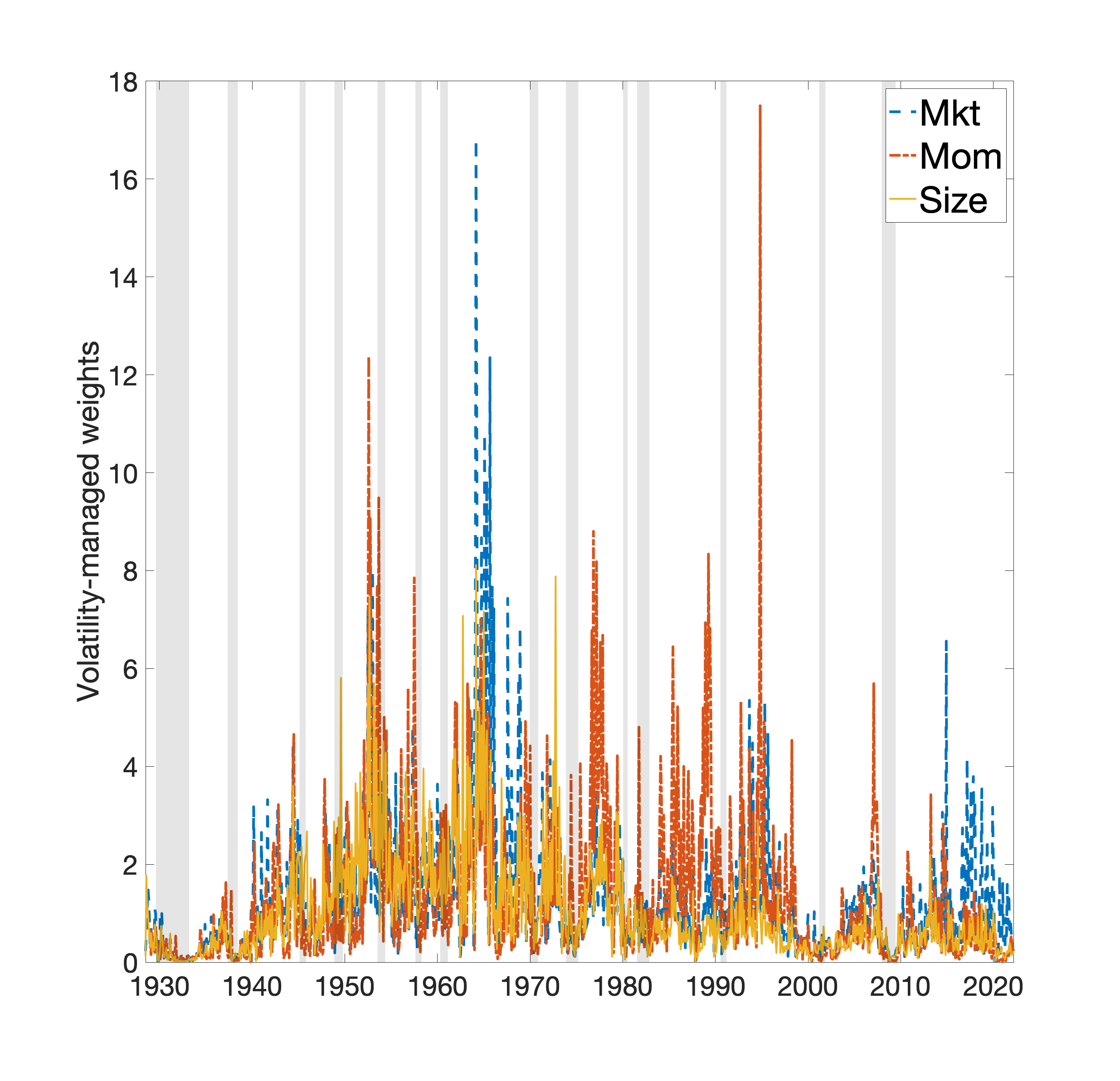
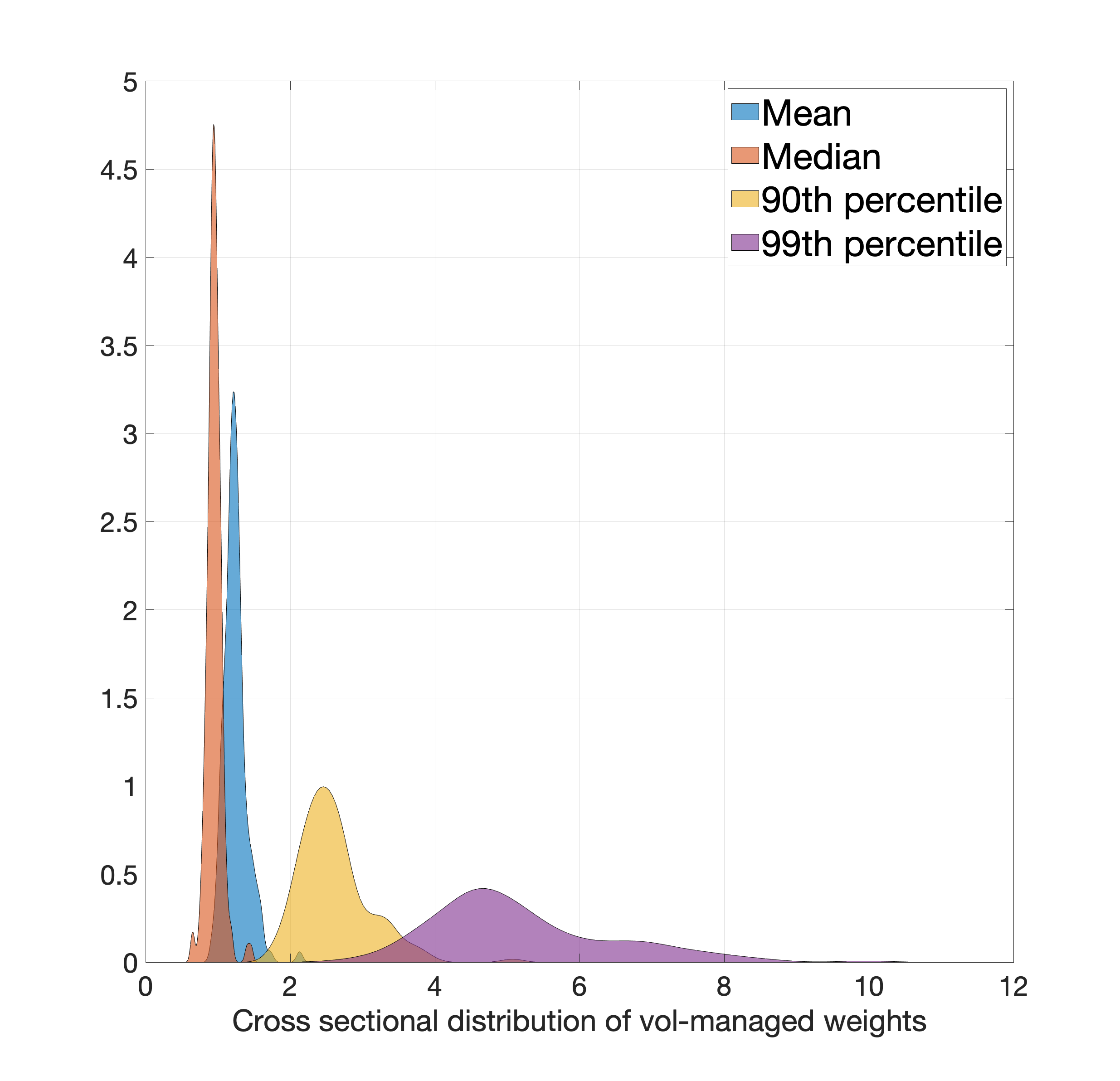
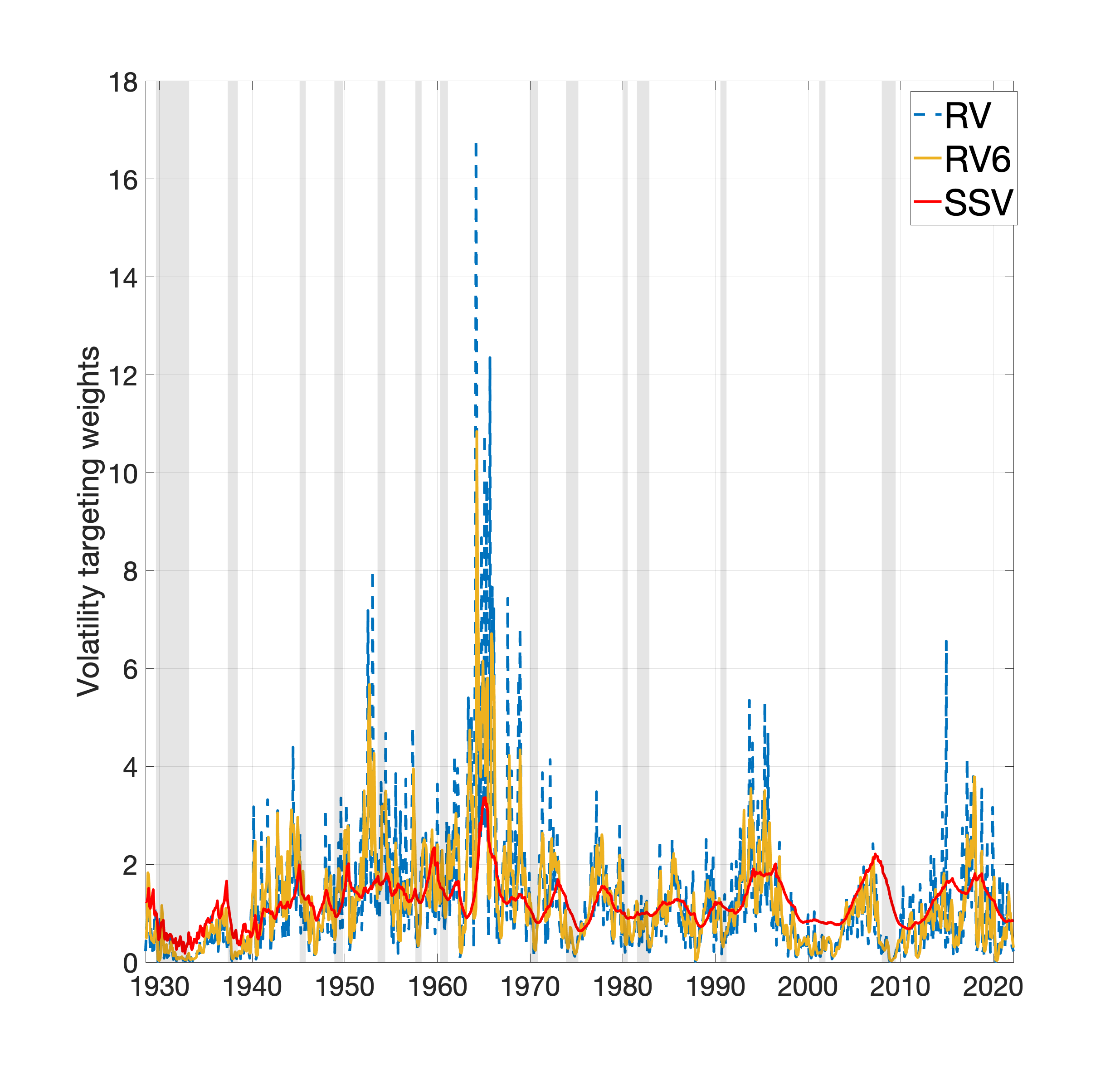
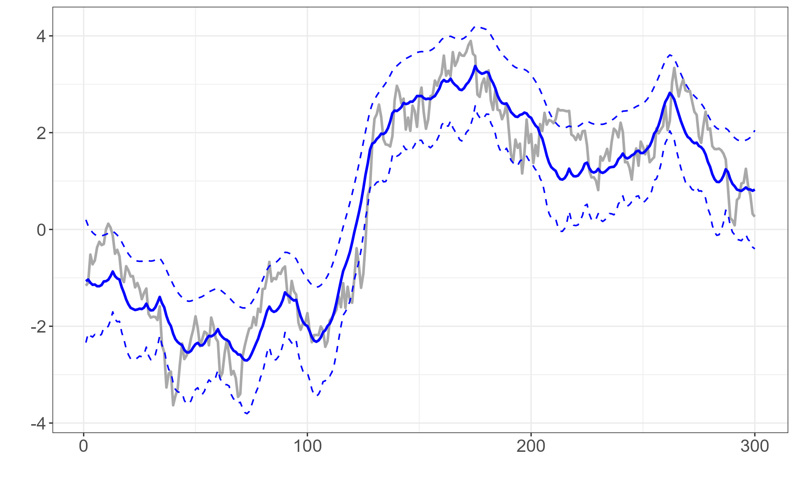
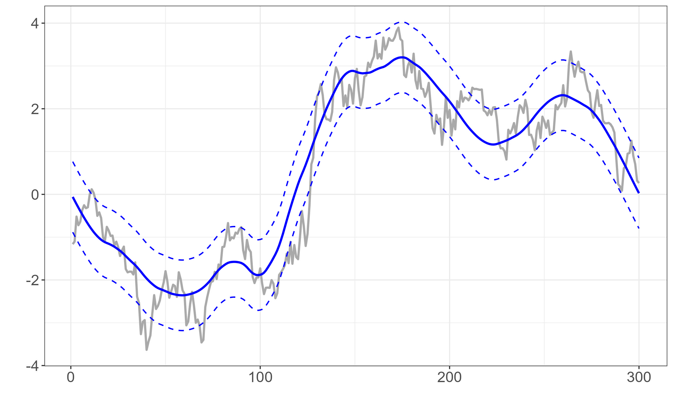
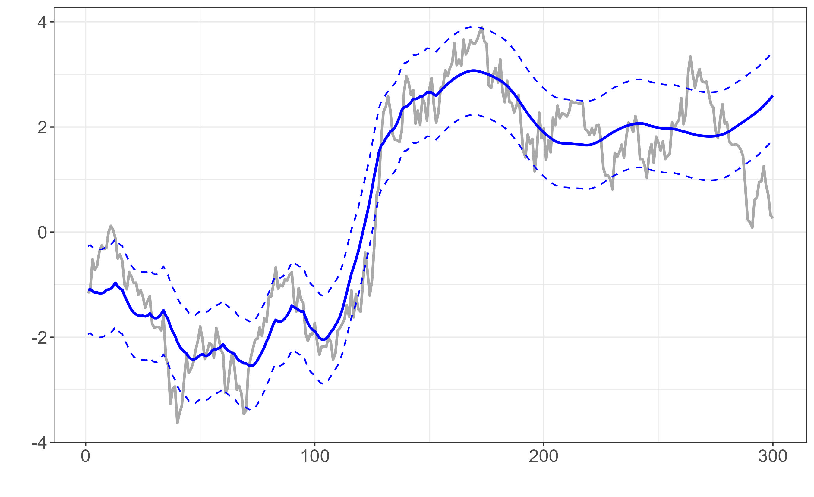
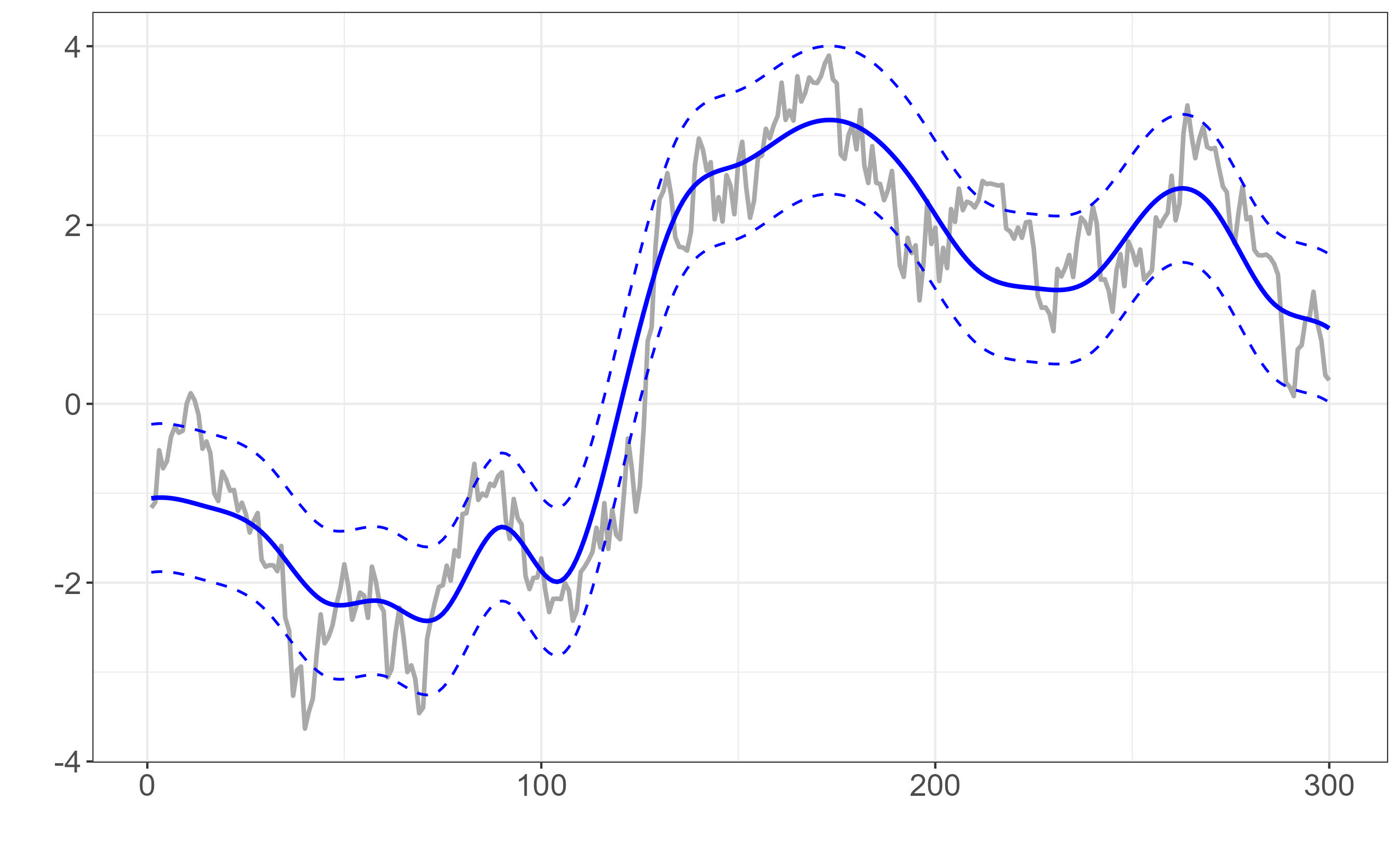
The form of $\mathbf{W}$ in case of wavelet basis functions (top) and B-spline basis functions (bottom). Right panels correspond to columns of the matrix $\mathbf{W}$. The B-spline basis functions is a sequence of piecewise polynomial functions of a given degree, in this case $dg=3$. The locations of the pieces are determined by the knots, here we assume $kn=20$ equally spaced knots. The functions that compose the wavelet basis matrix $\mathbf{W}$ are constructed over equally spaced grids on $[0,n]$ of length $R$, where $R$ is called resolution and it is equal to $2^{l-1}$, where $l$ defines the level (and in our case the resulting smoothness). The number of functions at level $l$ is then equal to $R$ and they are defined as dilatation and/or shift of a mother function. In our case the level is $l=5$ and therefore the resolution is $R=16$.

(a) Daubechies wavelet basis matrix

(b) Daubechies wavelet basis functions

(c) B-spline basis matrix with $kn=20$ and $dg=3$

(d) B-spline basis functions

Figure 4: Testing the significance of volatility-managed returns

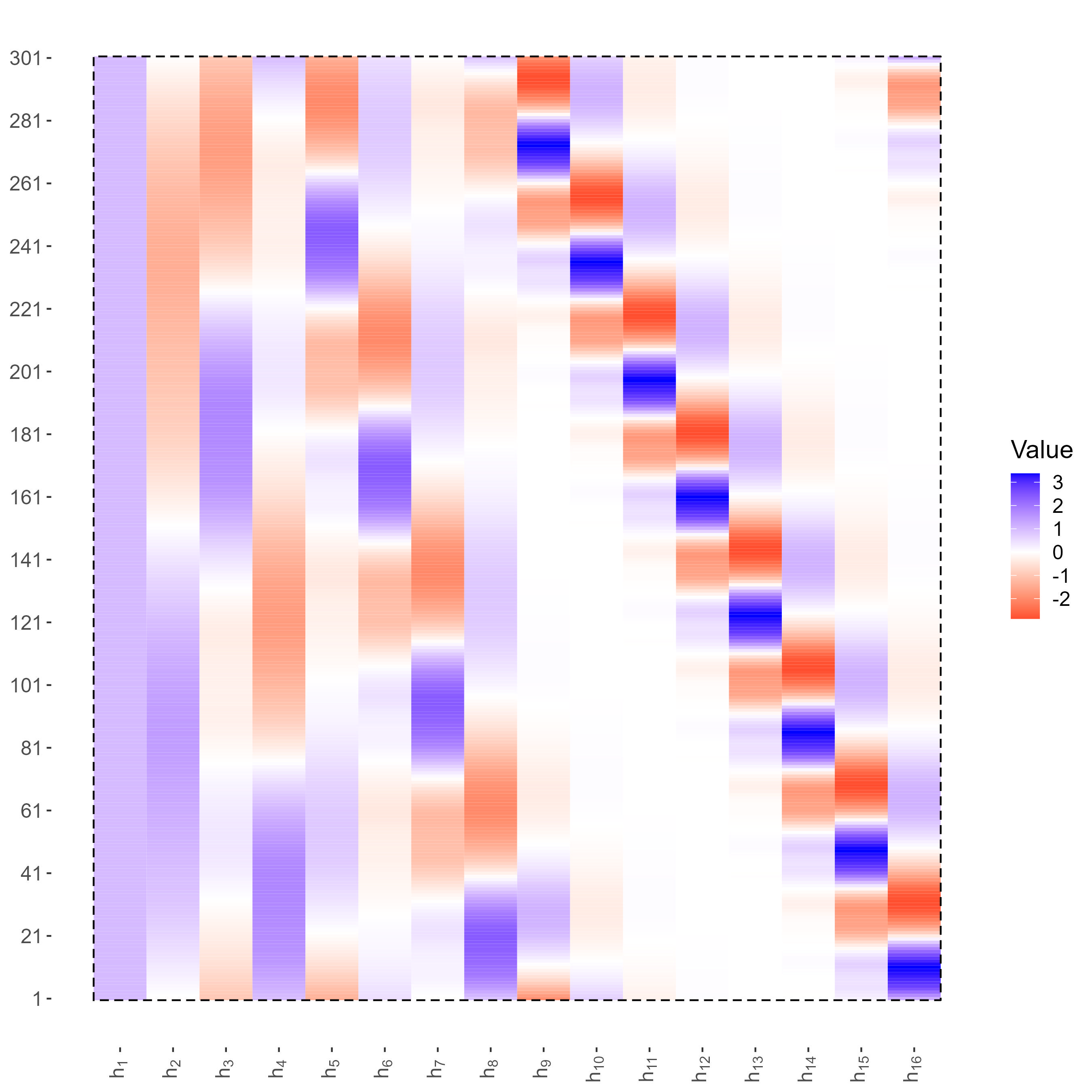
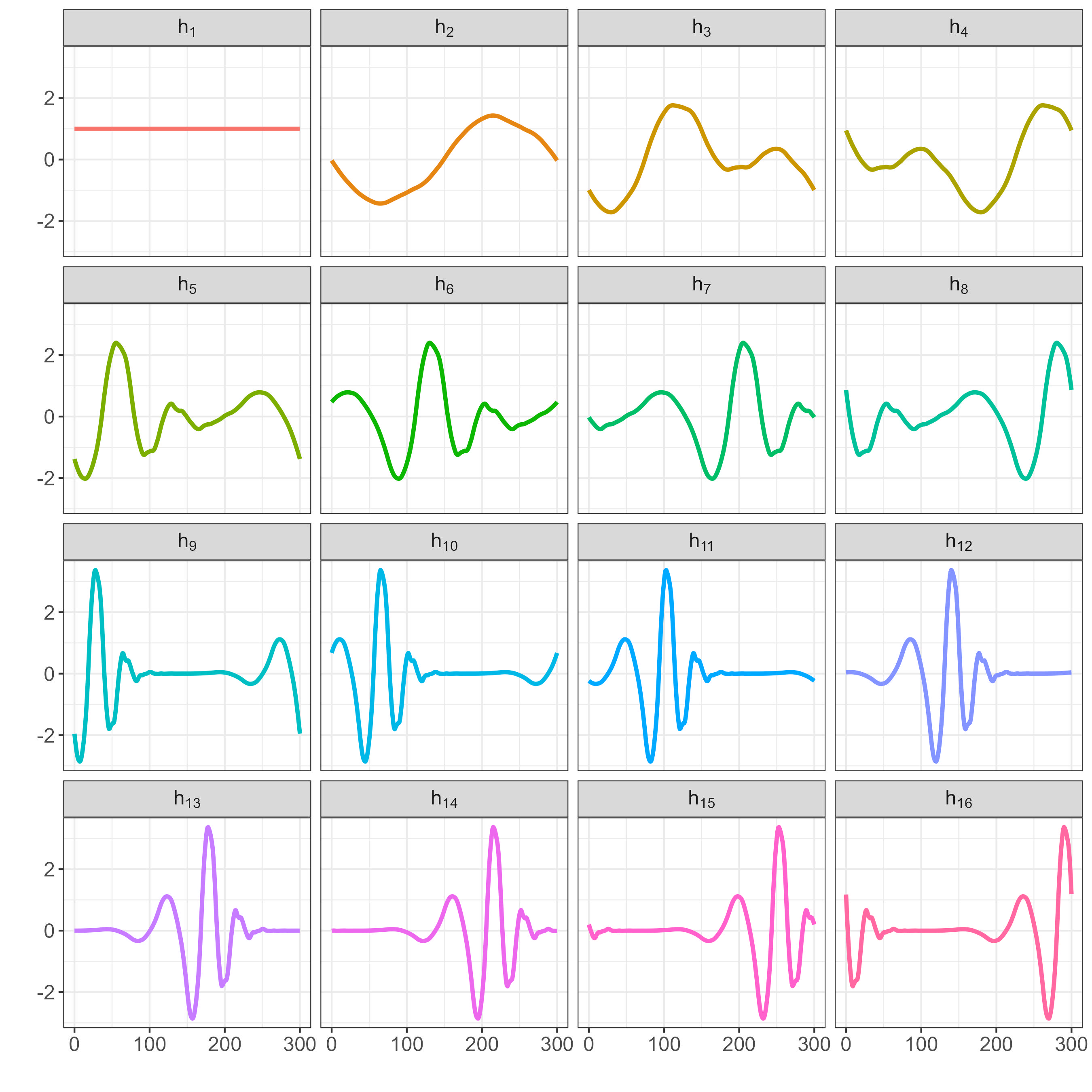
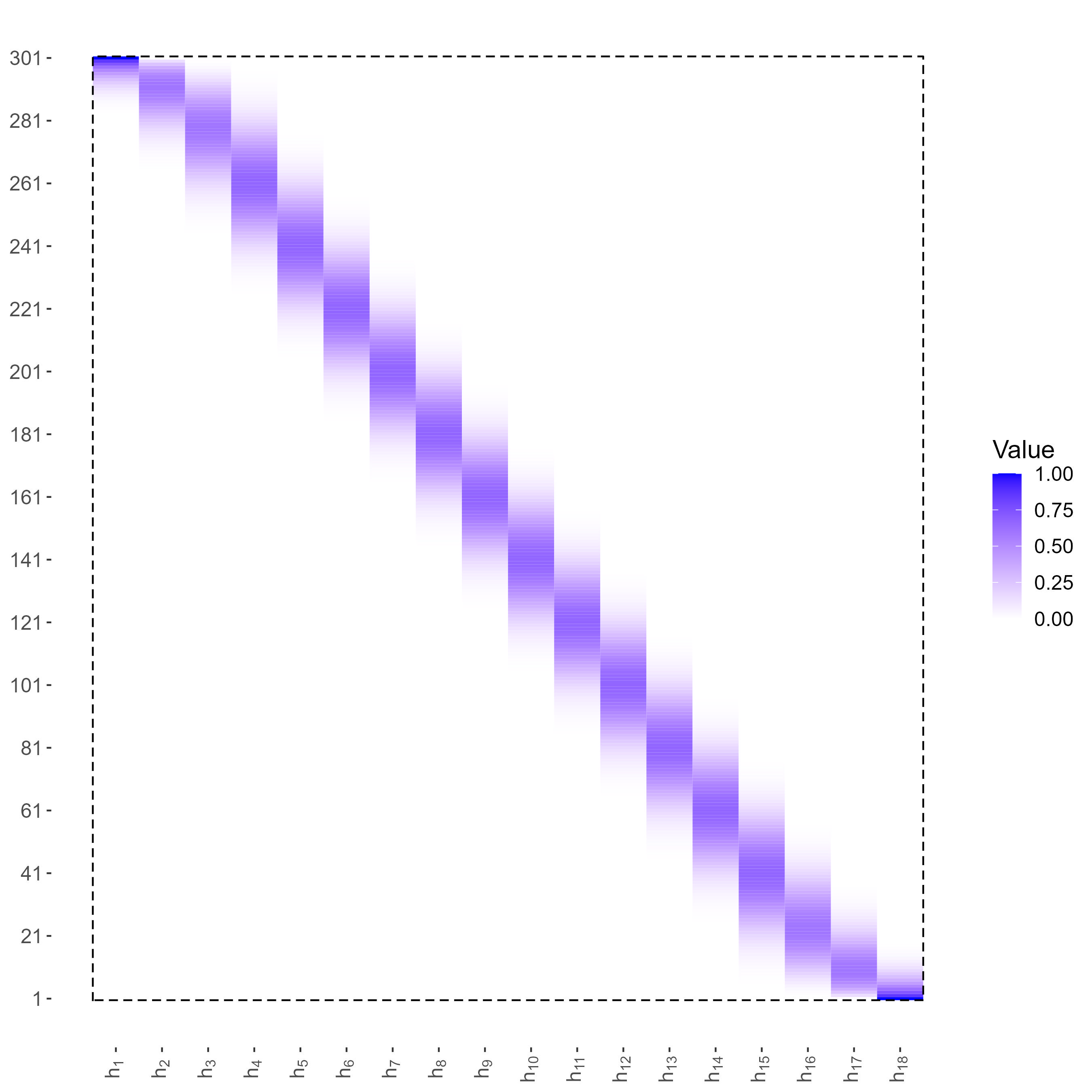
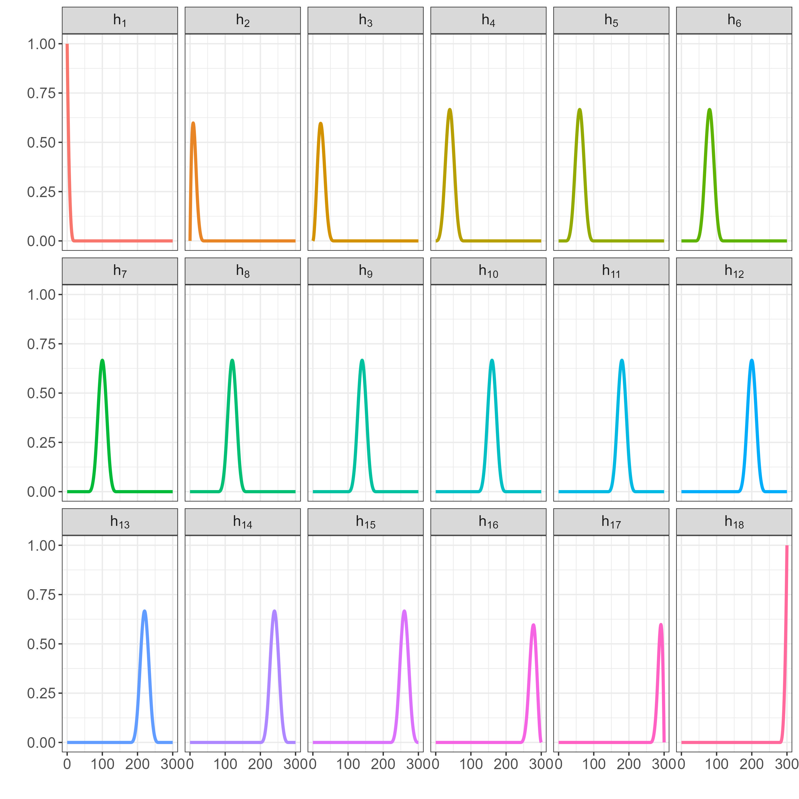
The plot reports the distribution of the volatility-managed portfolio returns implied by the non-smooth SV (red area) and smooth SSV (blue area) stochastic volatility models. We report a snapshot of the returns distribution on a given month for the market portfolio. The realised volatility-managed returns from the unmanaged and the RV are highlighted each month as white and green circles, respectively. The distribution of the volatility-managed portfolios for the SV and SSV is generated based on the predictive density of the corresponding model specifications (see Section 2.1.2 for more details).

(a) MKT October 1995

(b) MKT March 2009

(c) Momentum factor over 2008/2009

Figure 5: Smoothing vs alternative volatility targeting for the full sample

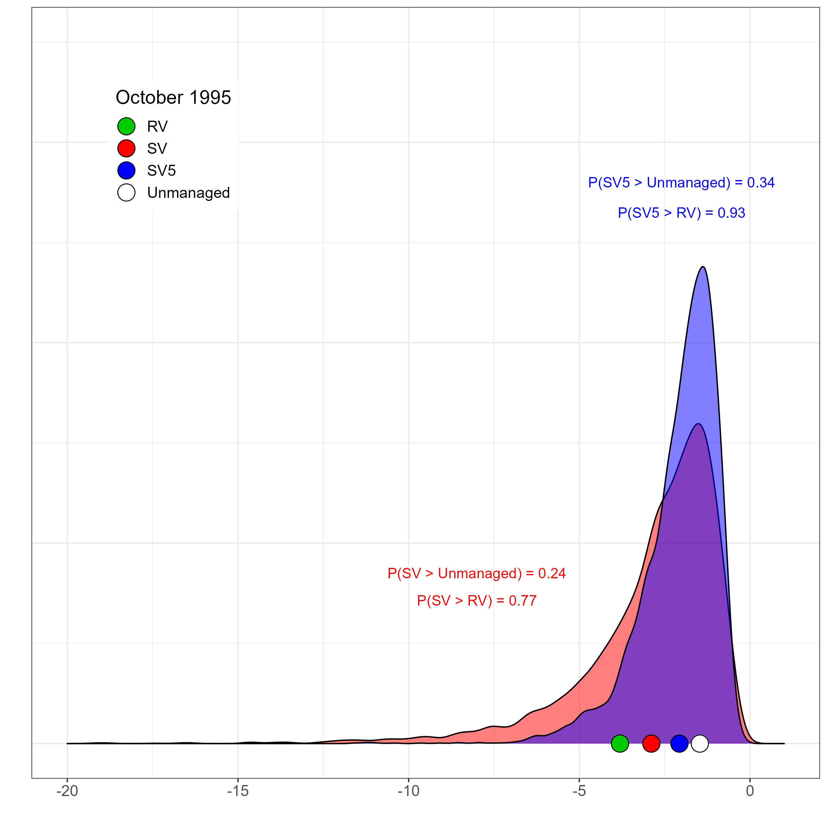
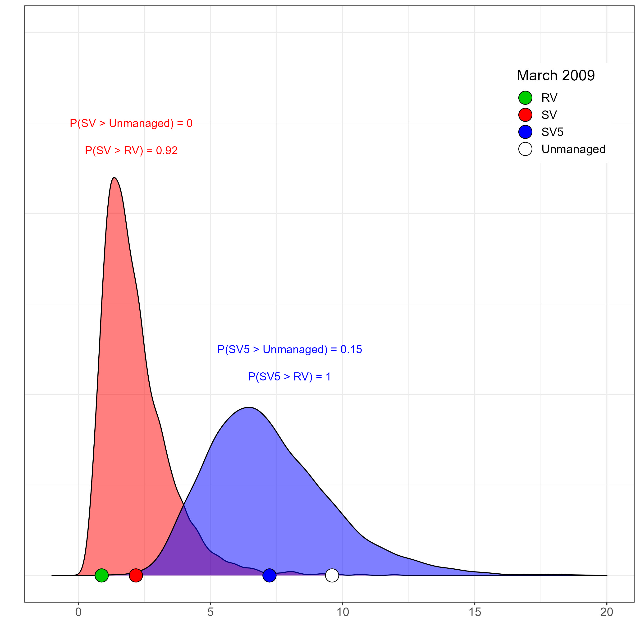
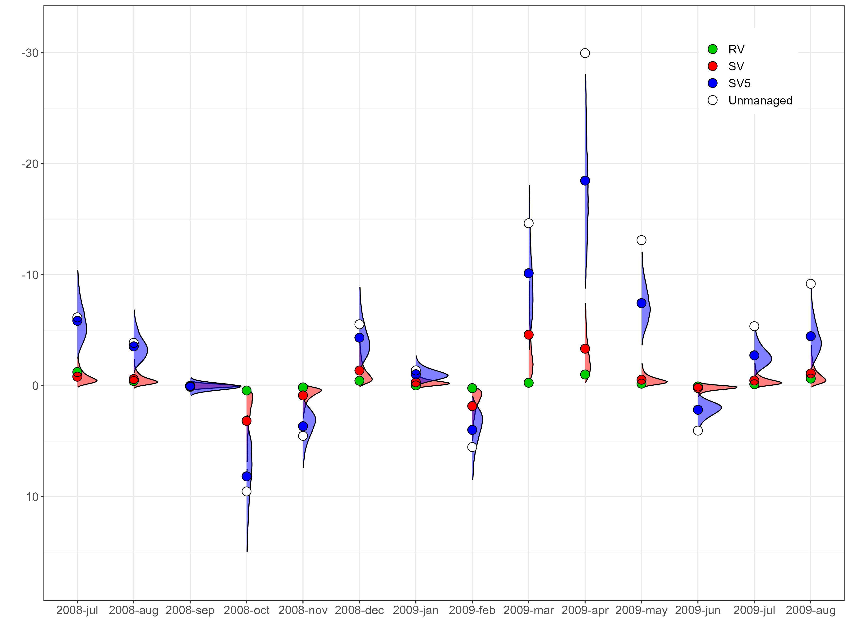
This figure reports the probability $p_{i}=p_{i}^{+}-p_{i}^{-}$ (see Eq.23) for the cross section of 158 equity trading strategy investigated in the main empirical application. The left panel compares our SSV versus U and RV. The middle panel compares our SSV against two alternative smoothing volatility forecasts used in the literature, i.e., RV6 and RV AR. The right panel compares out SSV against two popular volatility forecasting methods, such as HAR and Garch.

(a) $y_{t}^{{\tt SSV}}$ vs $y_{t}^{{\tt U}}$, $y_{t}^{{\tt RV}}$

(b) $y_{t}^{{\tt SSV}}$ vs $y_{t}^{{\tt RV6}}$, $y_{t}^{{\tt RVAR}}$

(c) $y_{t}^{{\tt SSV}}$ vs $y_{t}^{{\tt HAR}}$, $y_{t}^{{\tt Garch}}$

Figure 6: Smoothing vs alternative volatility targeting over time

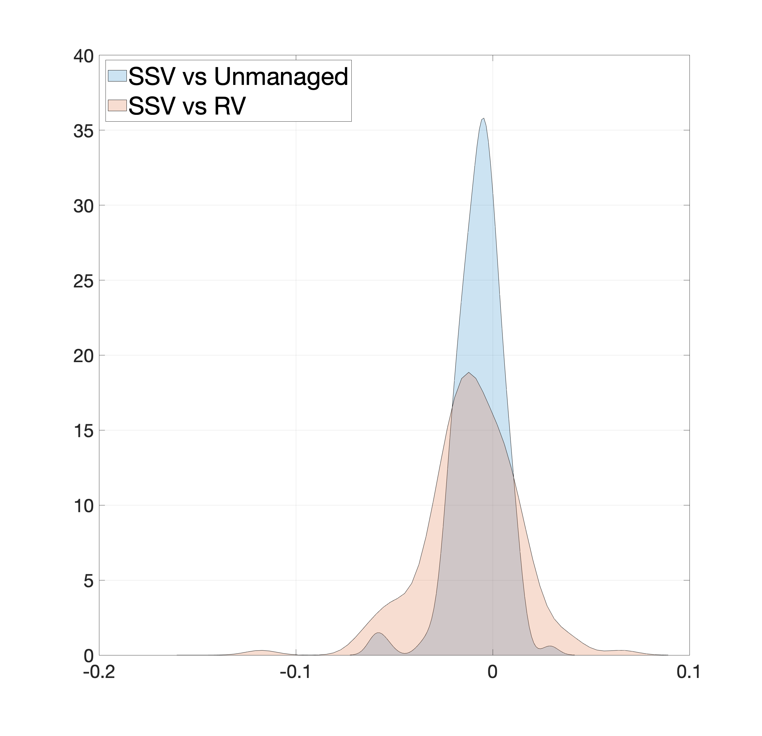
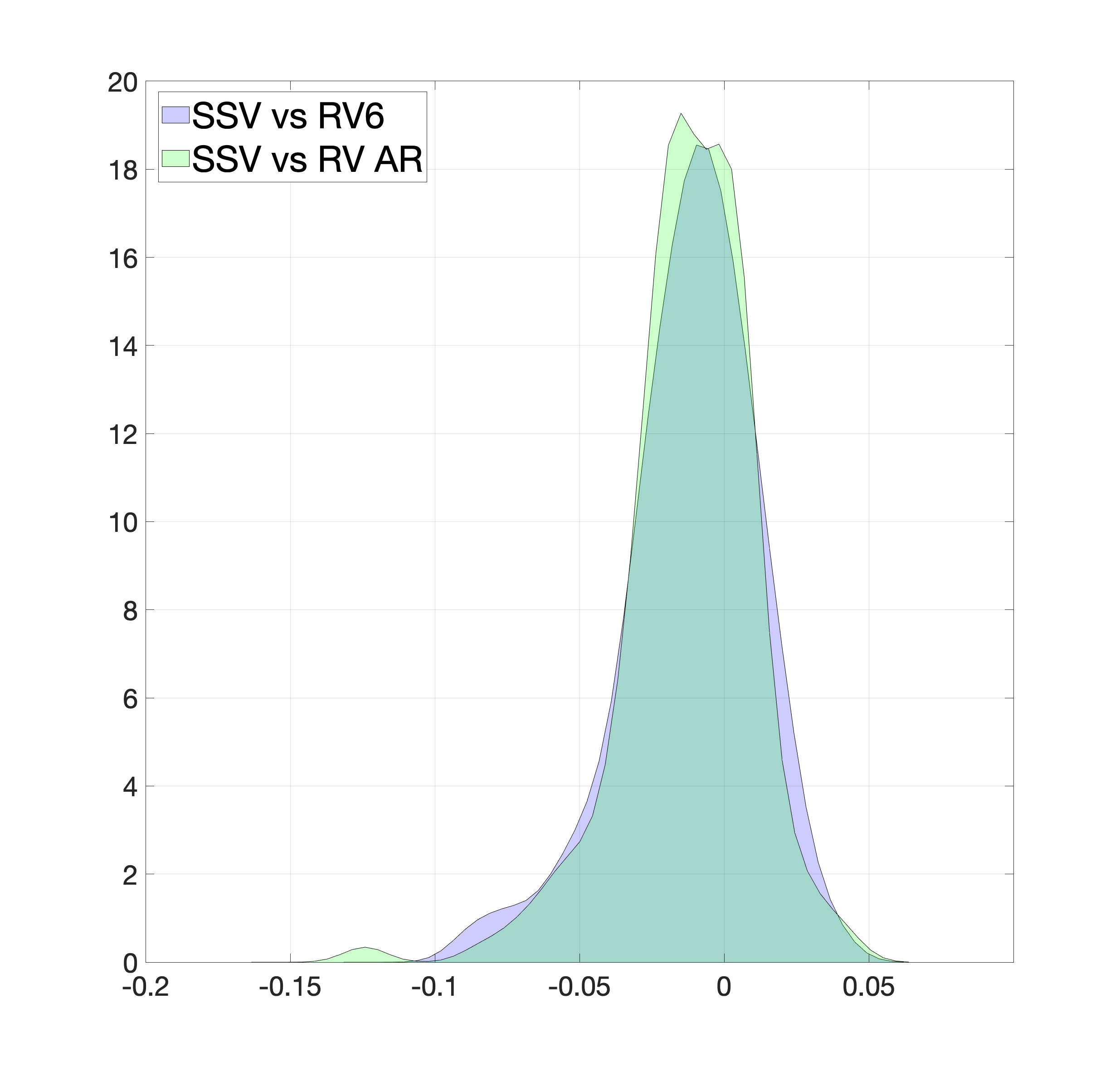
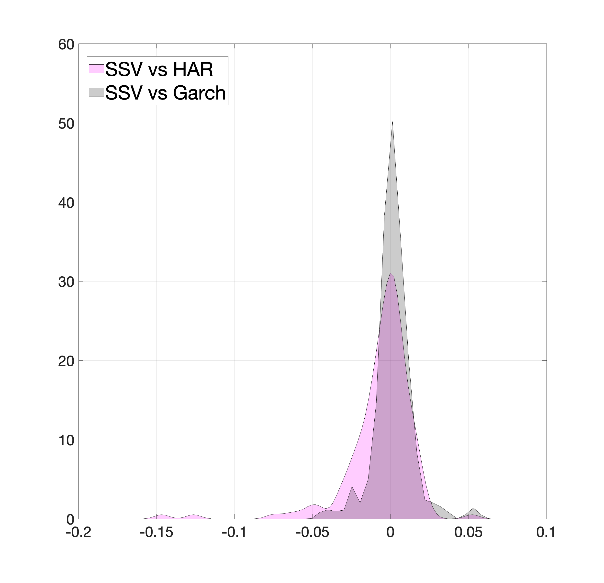
This figure reports the probability $p_{t}=p_{t}^{+}-p_{t}^{-}$ (see Eq.23) for the sample period under investigation. The left panel compares our SSV versus U and RV. The middle panel compares our SSV against two alternative smoothing volatility forecasts used in the literature, i.e., RV6 and RV AR. The right panel compares out SSV against two popular volatility forecasting methods, such as HAR and Garch.

(a) $y_{t}^{{\tt SSV}}$ vs $y_{t}^{{\tt U}}$, $y_{t}^{{\tt RV}}$

(b) $y_{t}^{{\tt SSV}}$ vs $y_{t}^{{\tt RV6}}$, $y_{t}^{{\tt RVAR}}$

(c) $y_{t}^{{\tt SSV}}$ vs $y_{t}^{{\tt HAR}}$, $y_{t}^{{\tt Garch}}$

Figure 7: Accuracy of the latent volatility estimates

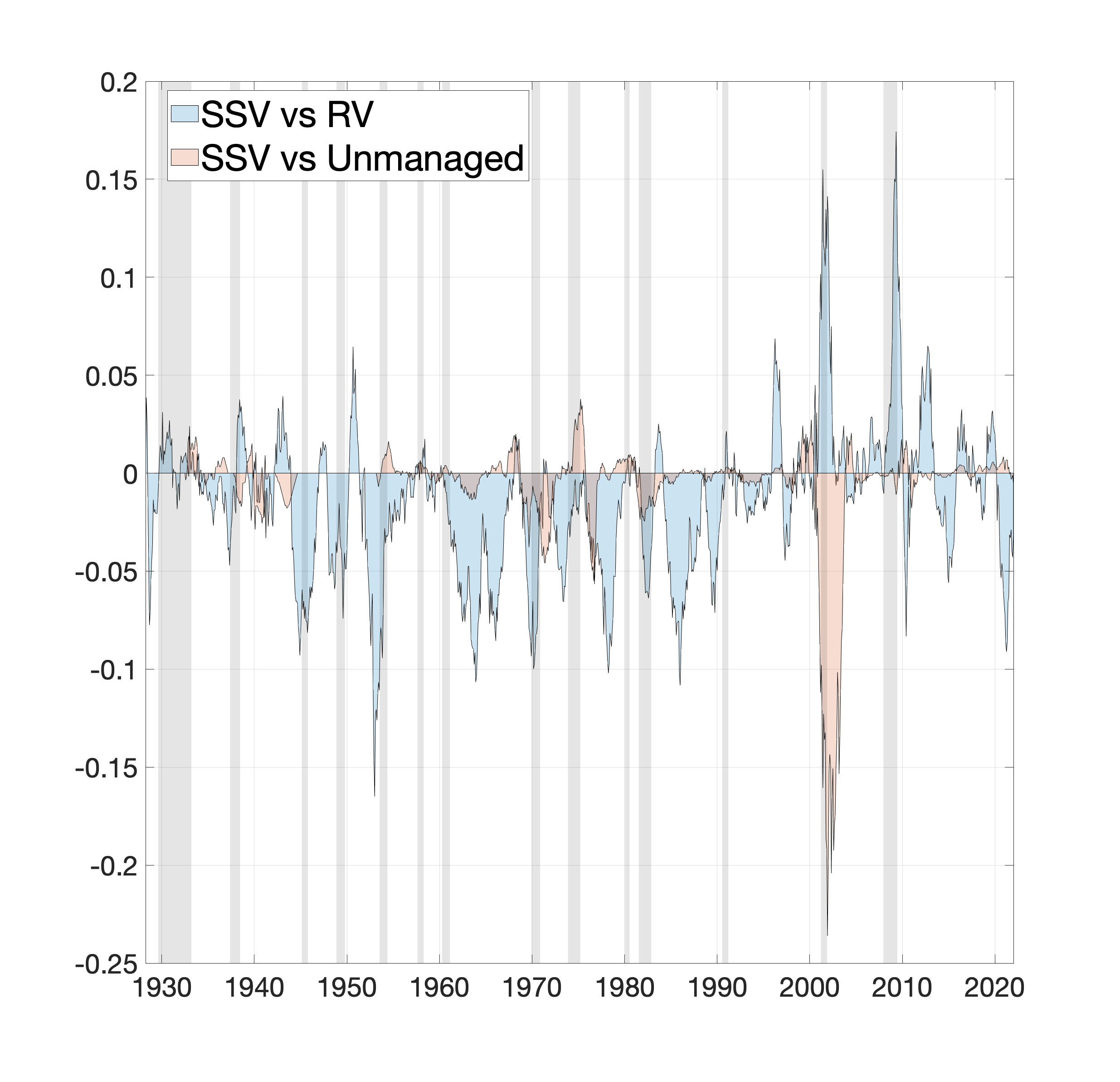
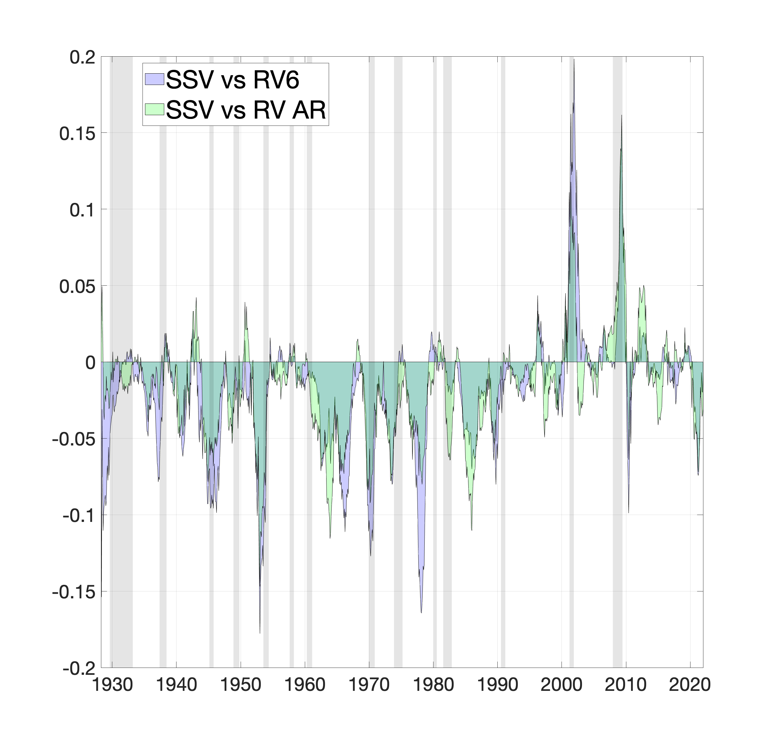
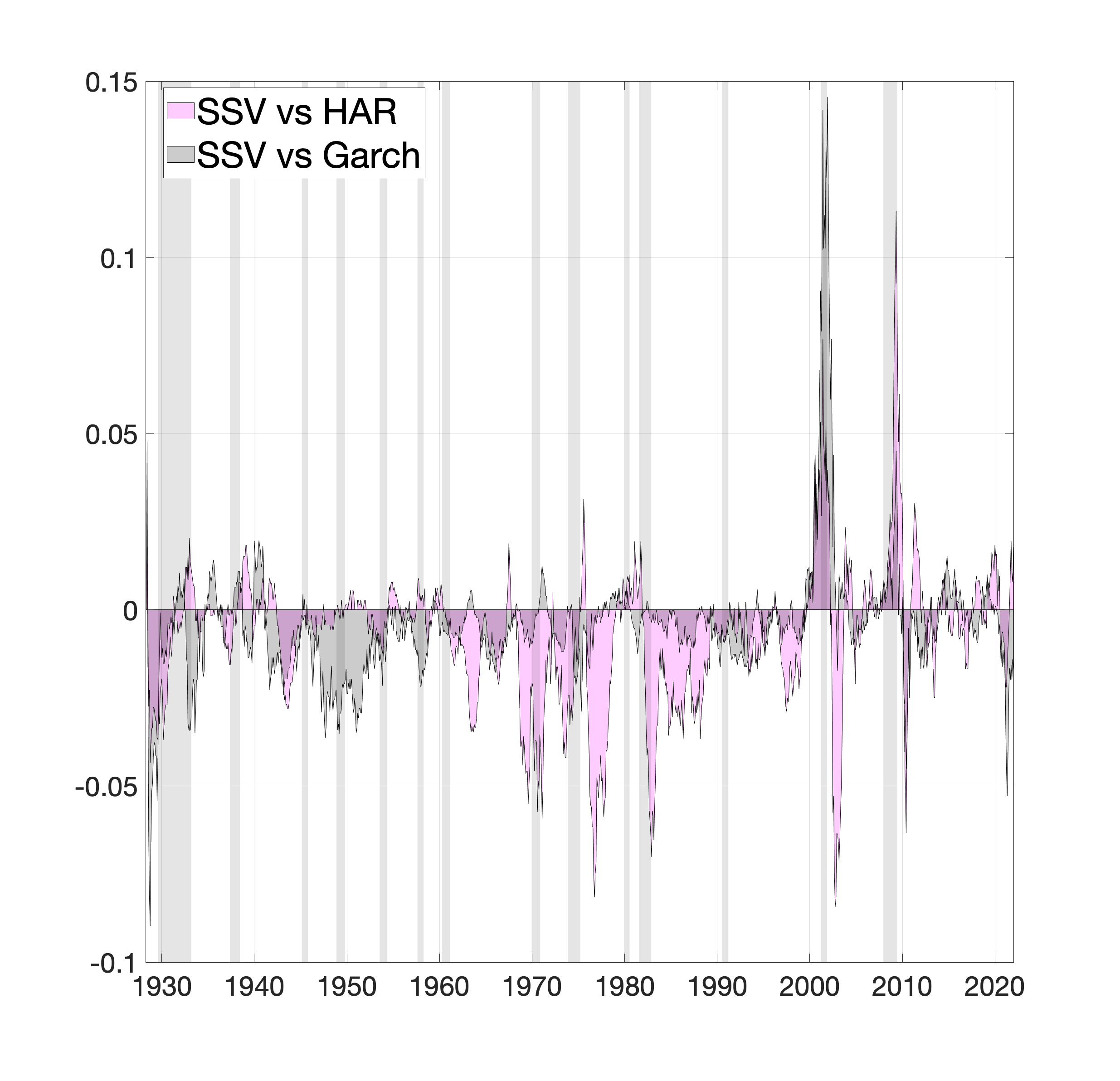
This figure reports the mean squared error and a measure of global estimation accuracy compared to the MCMC. The mean squared error is measured as $MSE=n^{-1}\sum_{t=1}^{n}(h_{t}-\hat{h}_{t})^{2}$, where $h_{t}$ and $\hat{h}$ are the simulated log-variance and its estimate, respectively. The global estimation accuracy compared to the MCMC is calculates as in Eq.(24). In addition, the left panels report the computational time across methods. We report the simulation results for both $\rho=0.98$ (top panels), and $\rho=0.7$ (bottom panels).

(a) MSE when $\rho=0.98$

(b) Global acc. when $\rho=0.98$

(c) Comp. time when $\rho=0.98$

(d) MSE when $\rho=0.70$

(e) Global acc. when $\rho=0.70$

(f) Comp. time when $\rho=0.70$

Figure 8: Estimates for the latent process parameters

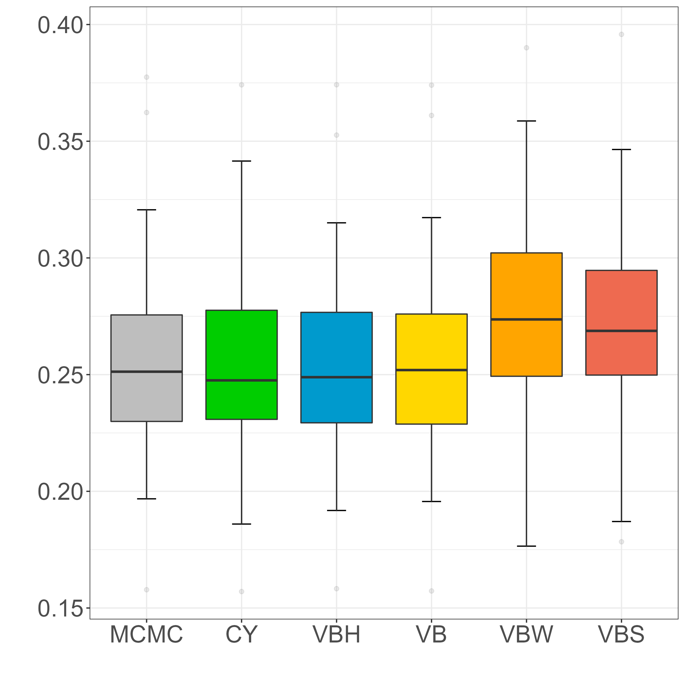
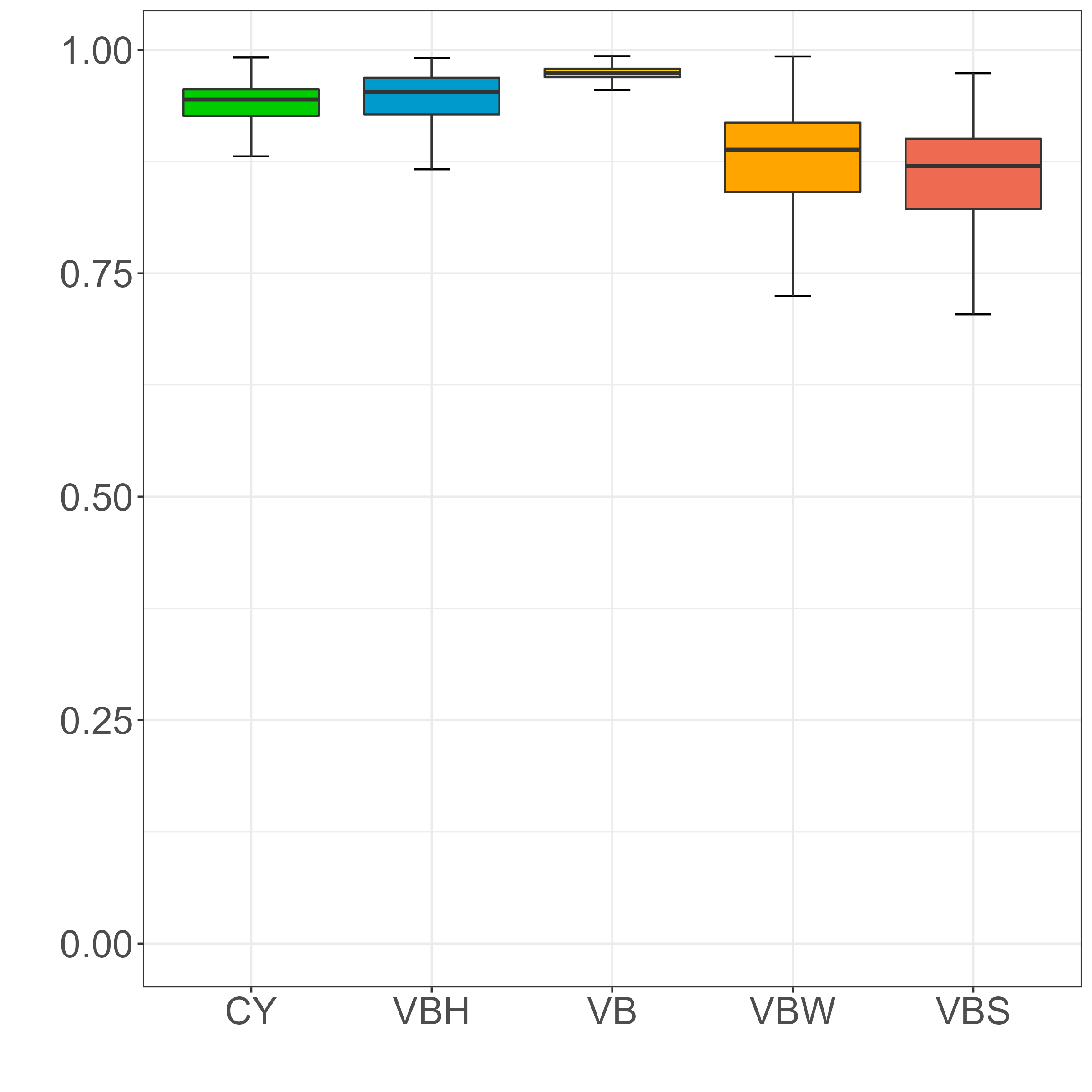
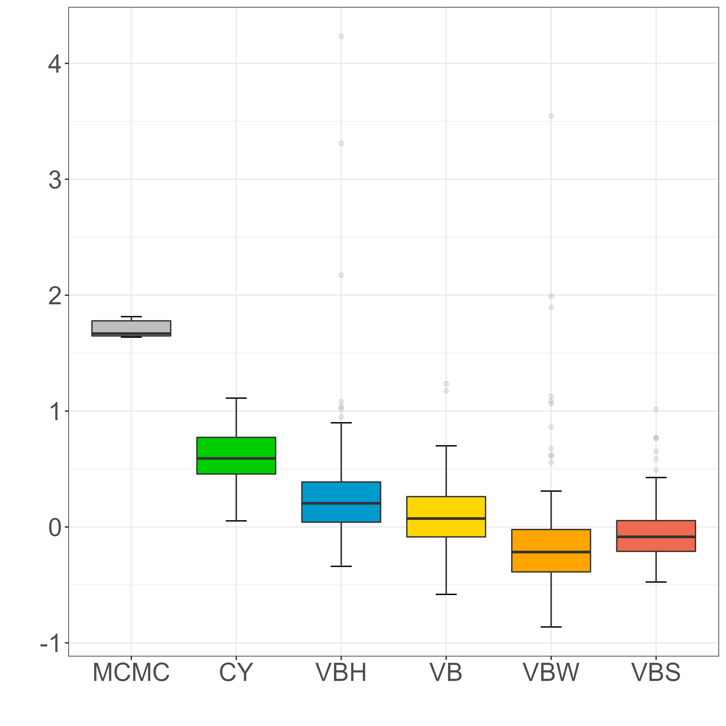
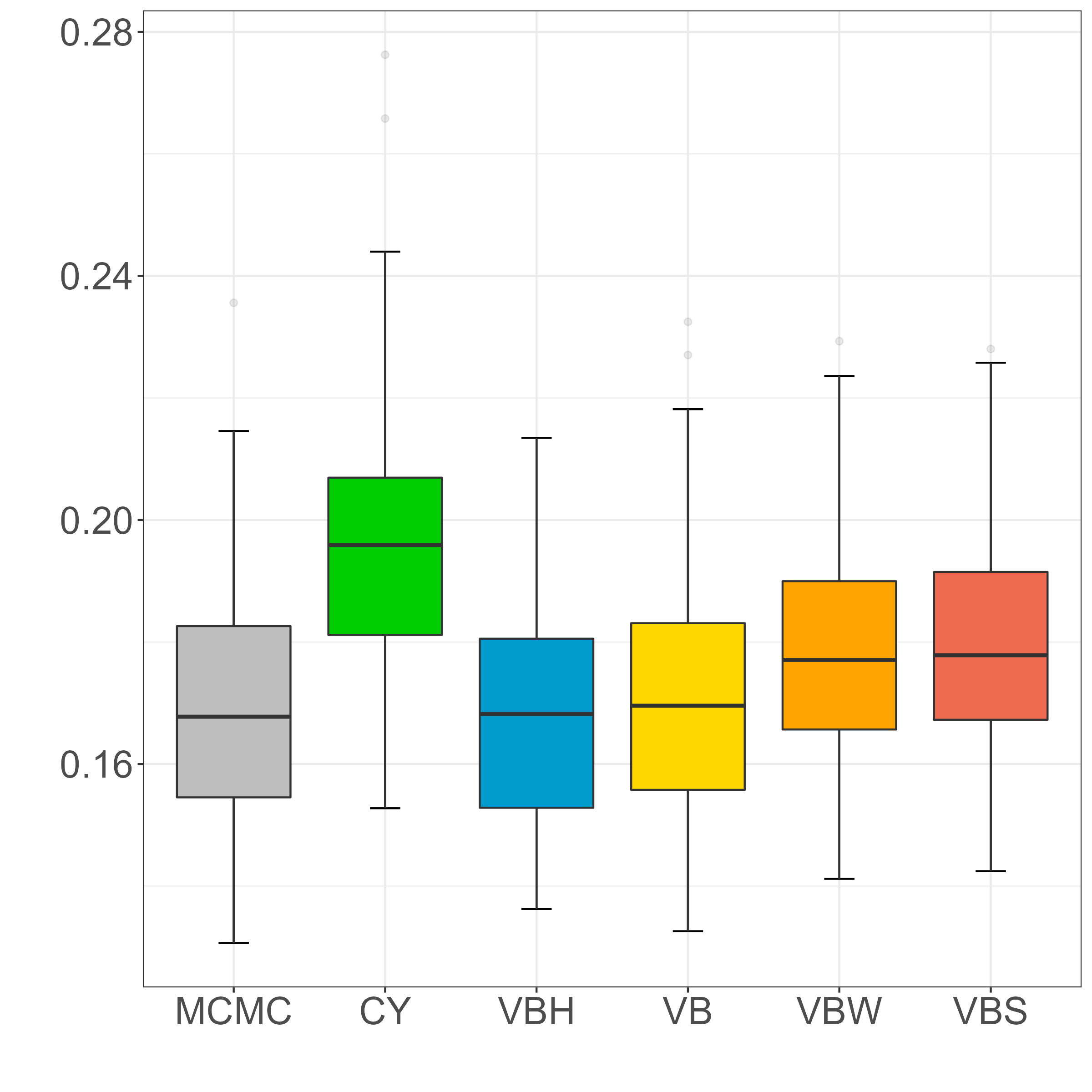
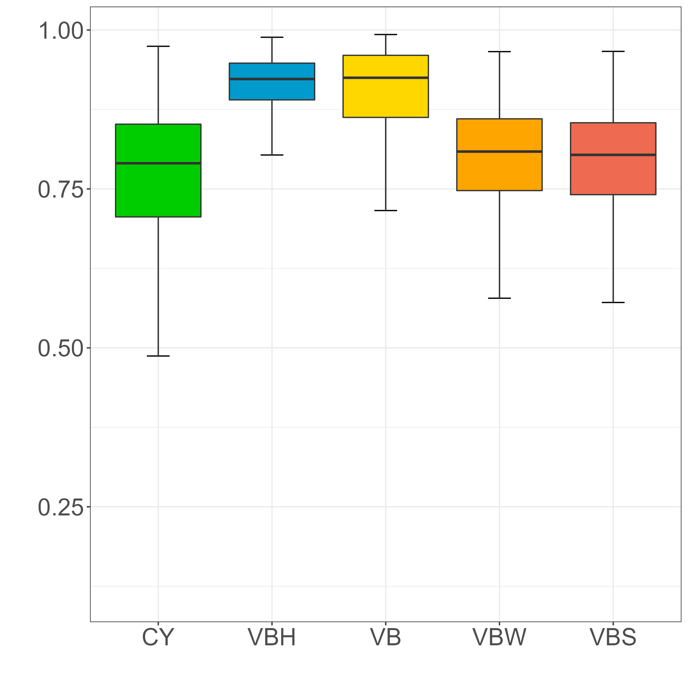
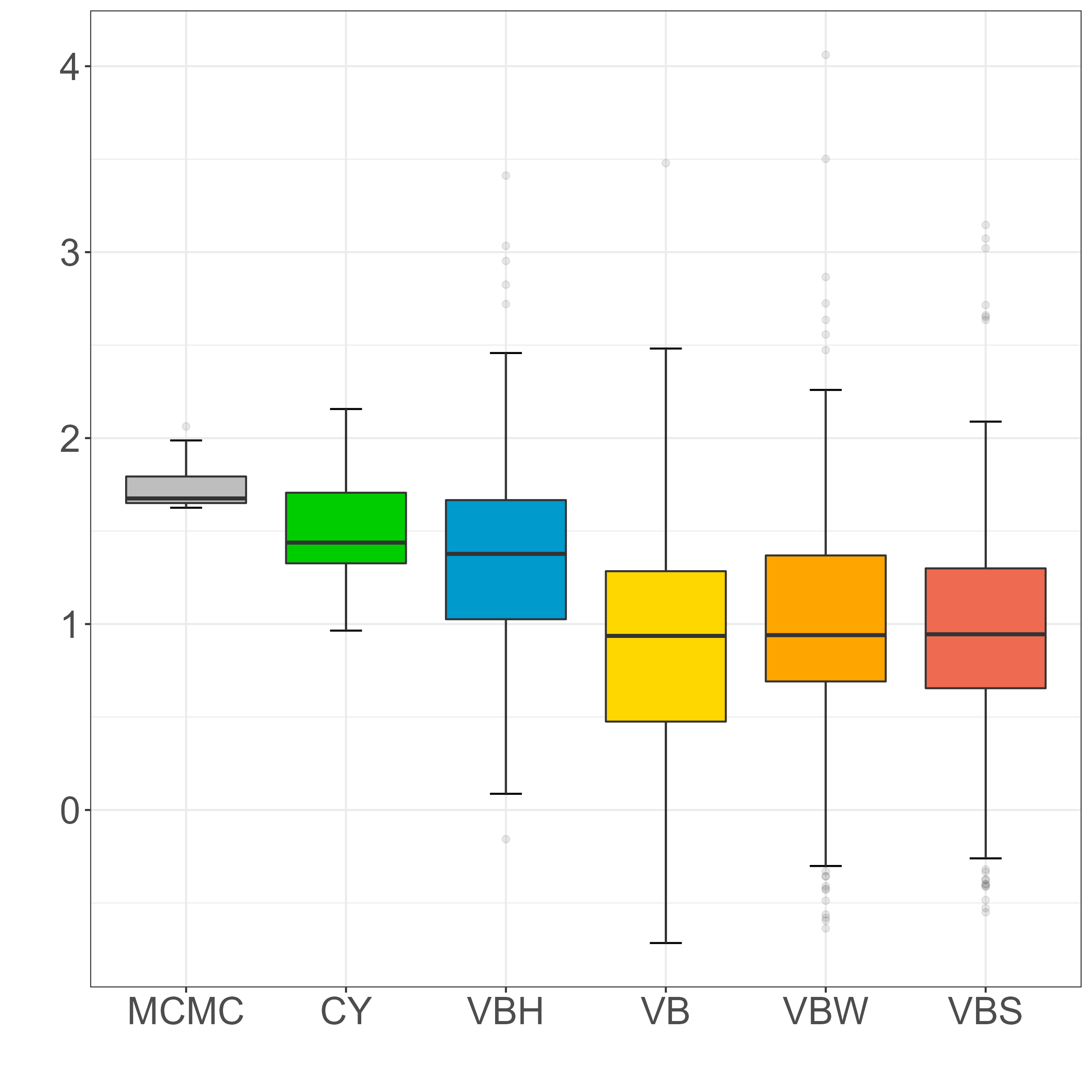
This figure reports the posterior estimates of the parameters of interest for the stochastic volatility models across simulations, and for different inference methods. We report the simulation results for both $\rho=0.98$ (top panels), and $\rho=0.7$ (bottom panels). We compare our variational Bayes methods, with and without smoothing, against both a standard MCMC (see Hosszejni and Kastner, 2021), and a global approximation method as proposed by Chan and Yu (2022).

(a) $\hat{c}$ when $\rho=0.98$

(b) $\hat{\eta}^{2}$ when $\rho=0.98$

(c) $\hat{\rho}$ when $\rho=0.98$

(d) $\hat{c}$ when $\rho=0.70$

(e) $\hat{\eta}^{2}$ when $\rho=0.70$

(f) $\hat{\rho}$ when $\rho=0.70$

Figure 9: Accuracy of approximations compared to MCMC approach at each time.

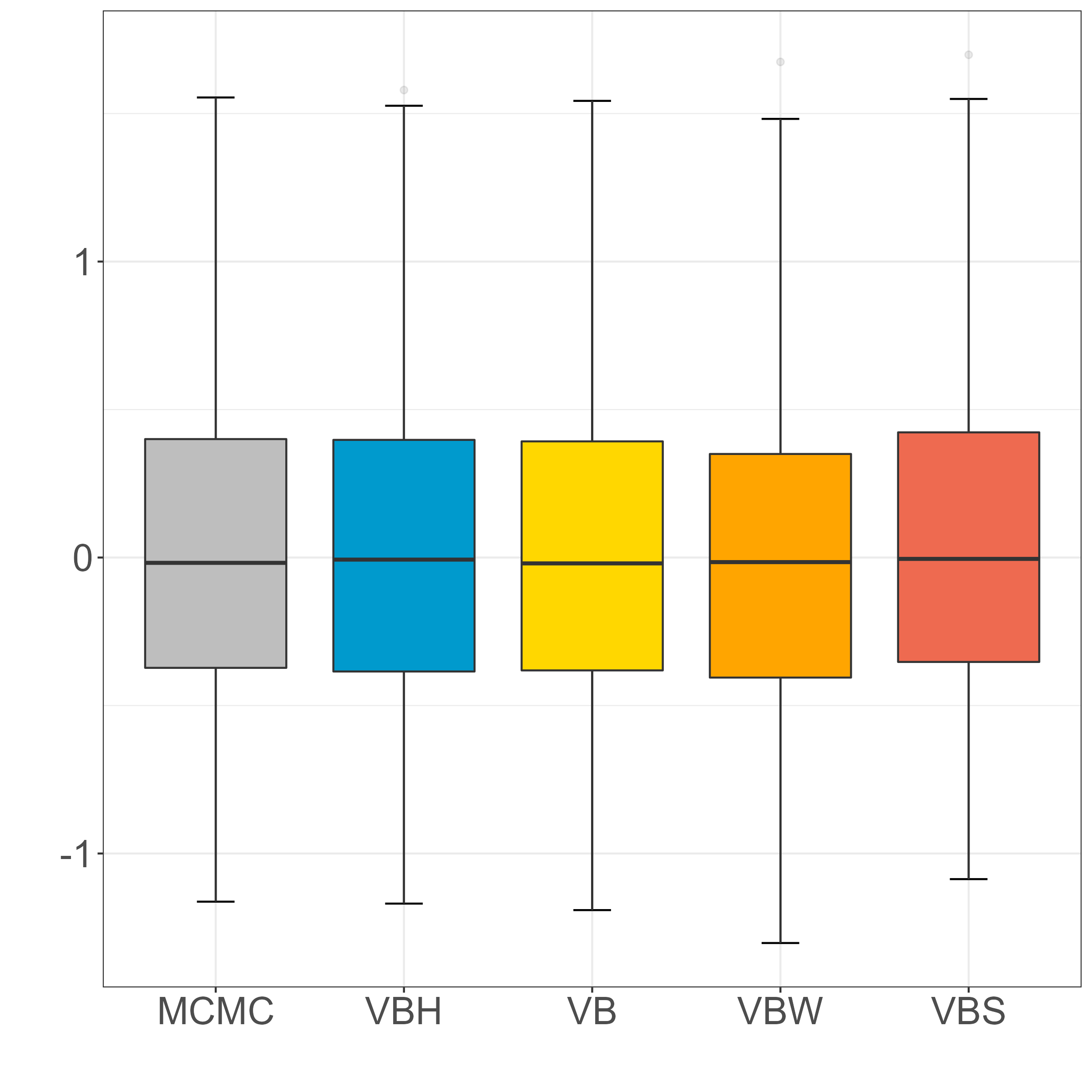
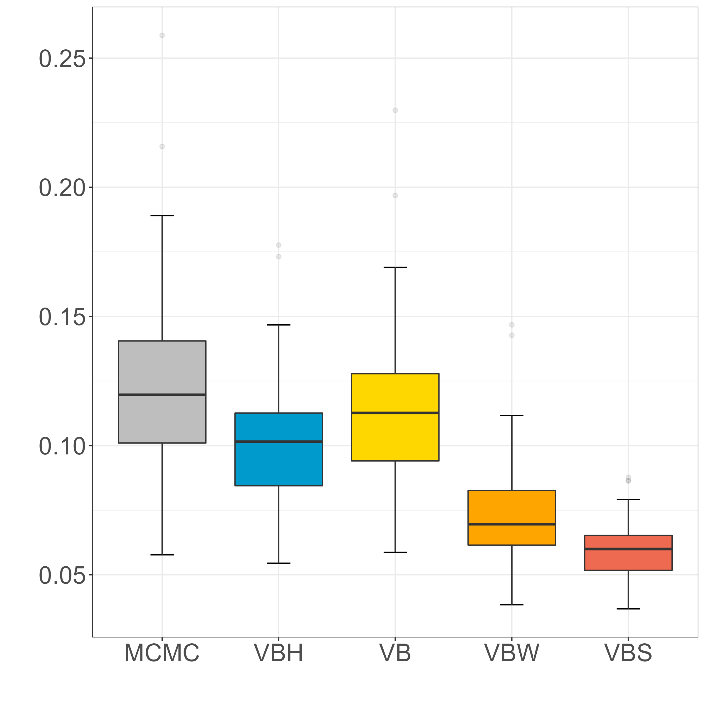
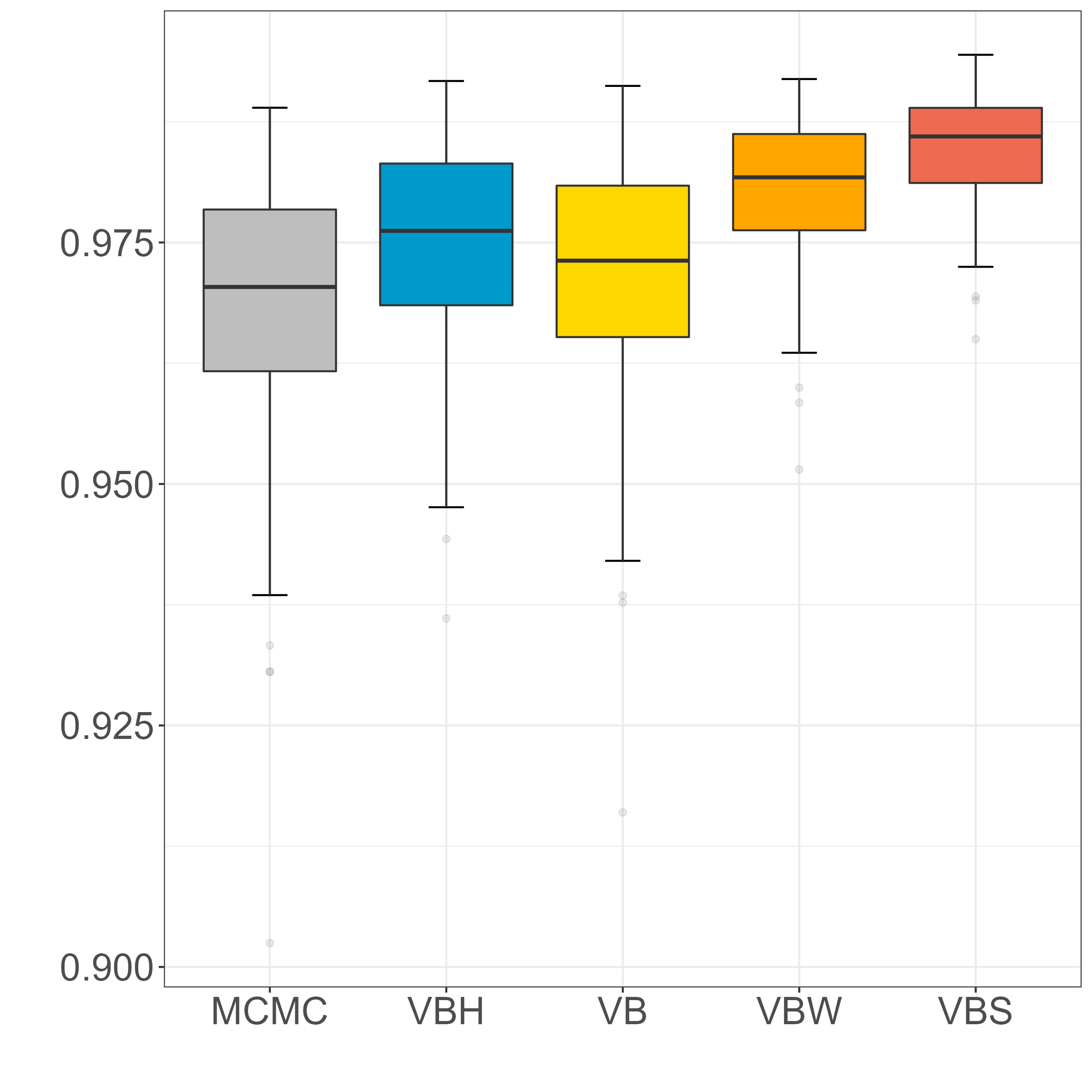
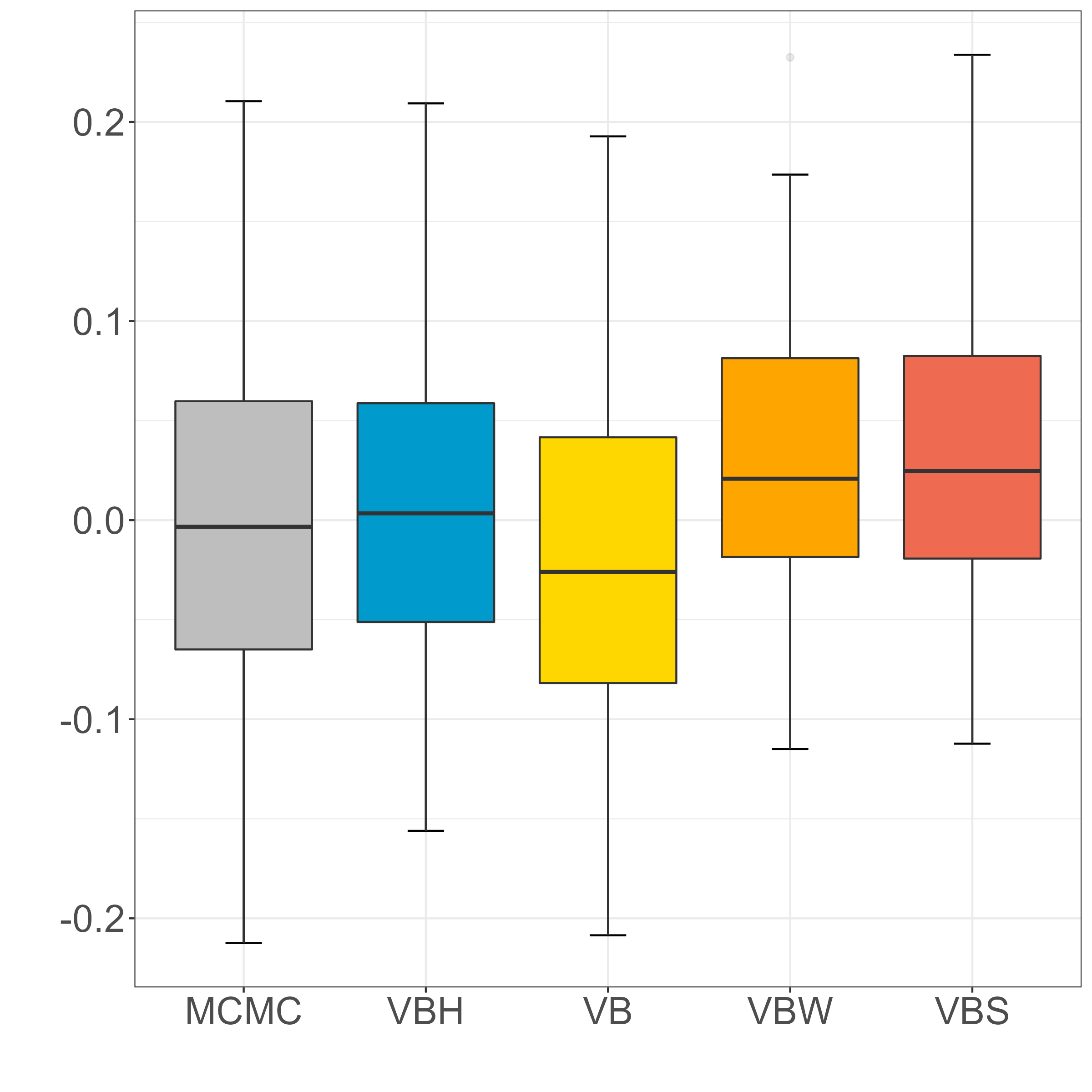
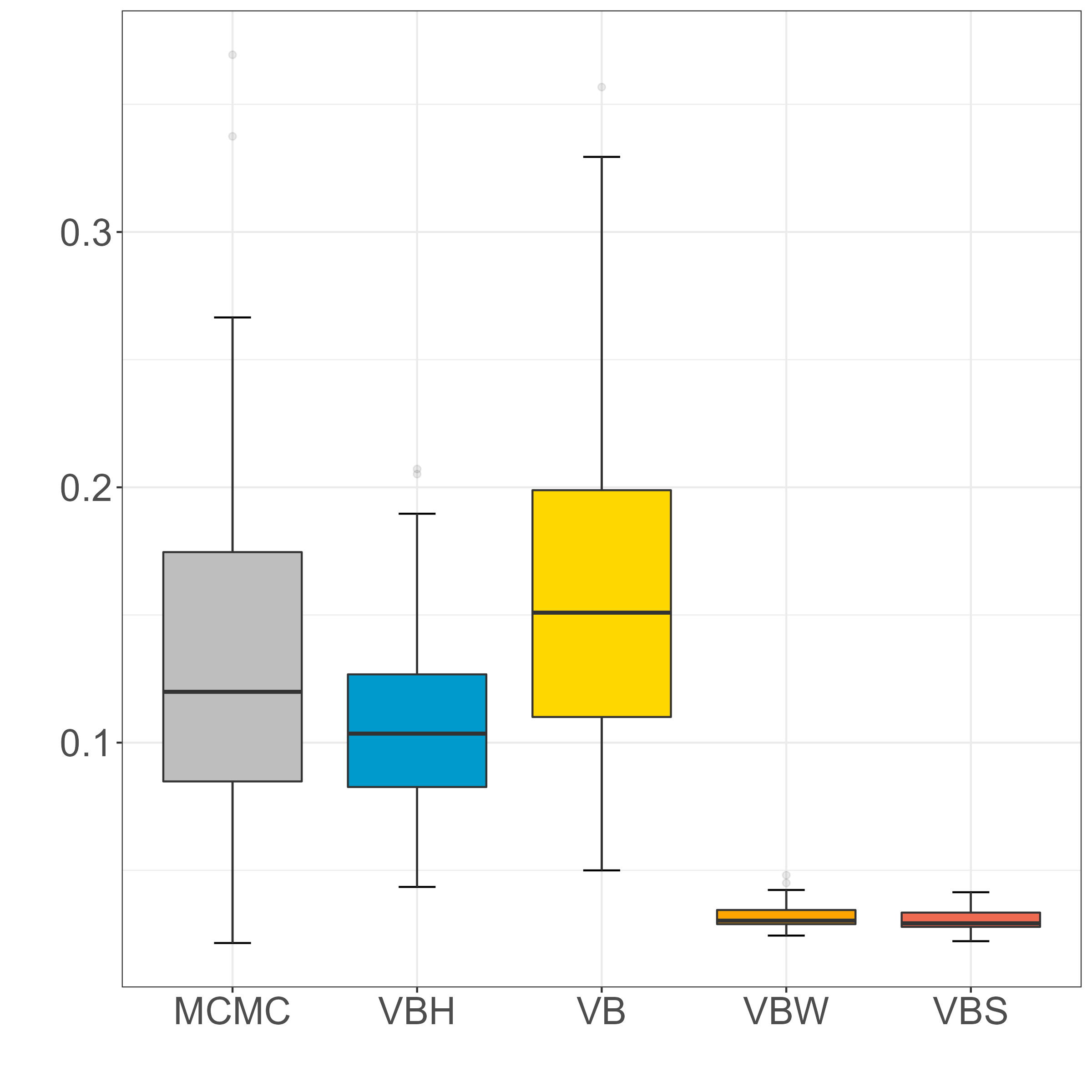
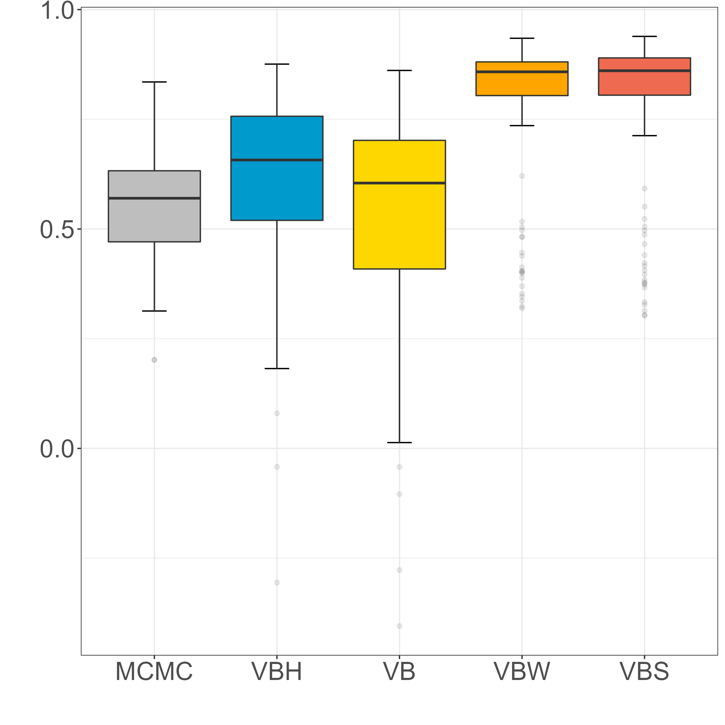
This figure reports the accuracy of our variational Bayes inference method against the global approximation method proposed by Chan and Yu (2022). The top (bottom) panels report the global accuracy when $\rho=0.98$ ($\rho=0.7$). We report the estimation results for $t\in\left(1,10\right)$ in the left panel, $t\in\left(301,310\right)$ in the middle panel, and $t\in\left(591,600\right)$ in the right panel. The accuracy is benchmarked against a standard MCMC method as in Hosszejni and Kastner (2021).

(a) $t\in(1,10)$ when $\rho=0.98$

(b) $t\in(301,310)$ when $\rho=0.98$

(c) $t\in(591,600)$ when $\rho=0.98$

(d) $t\in(1,10)$ when $\rho=0.70$

(e) $t\in(301,310)$ when $\rho=0.70$

(f) $t\in(591,600)$ when $\rho=0.70$

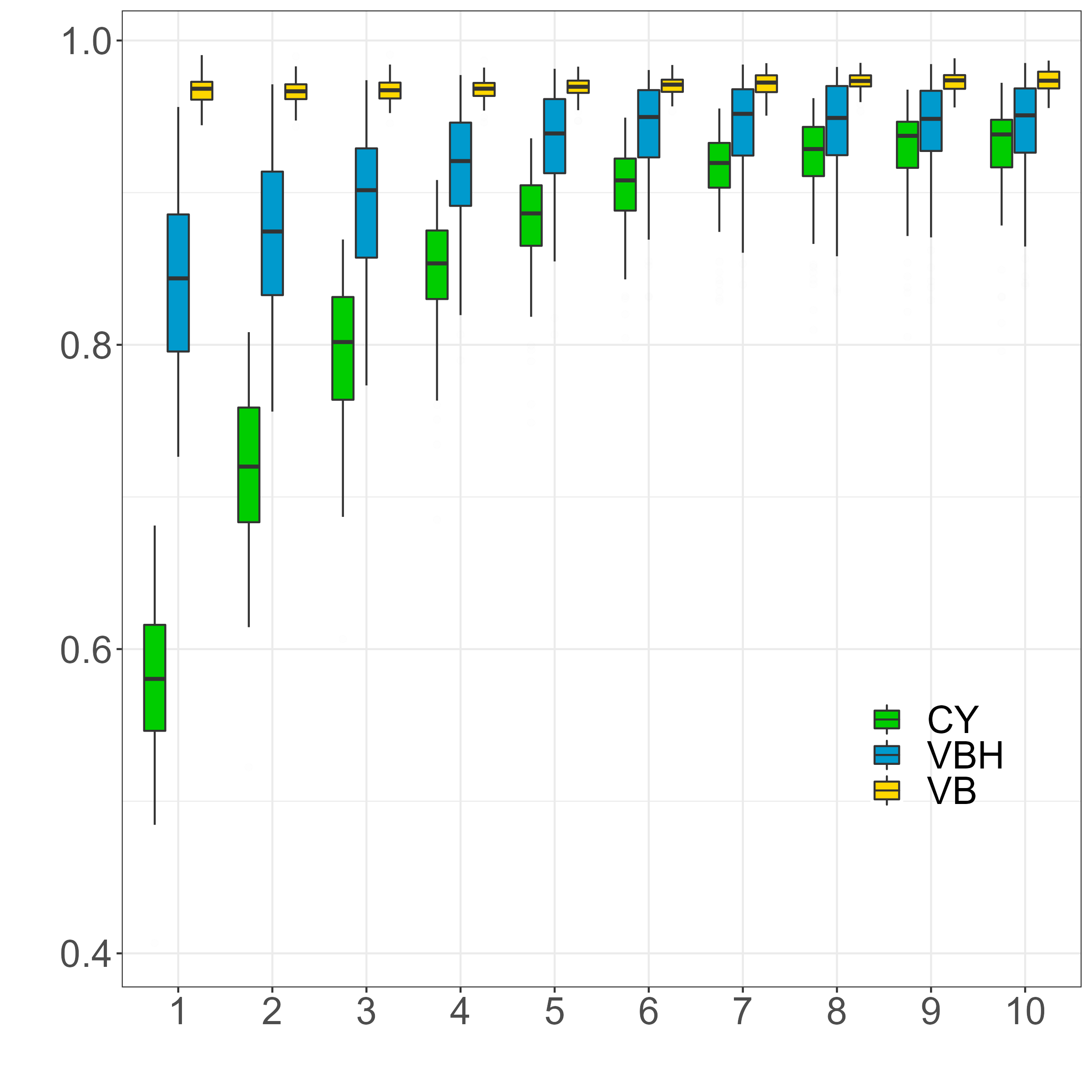
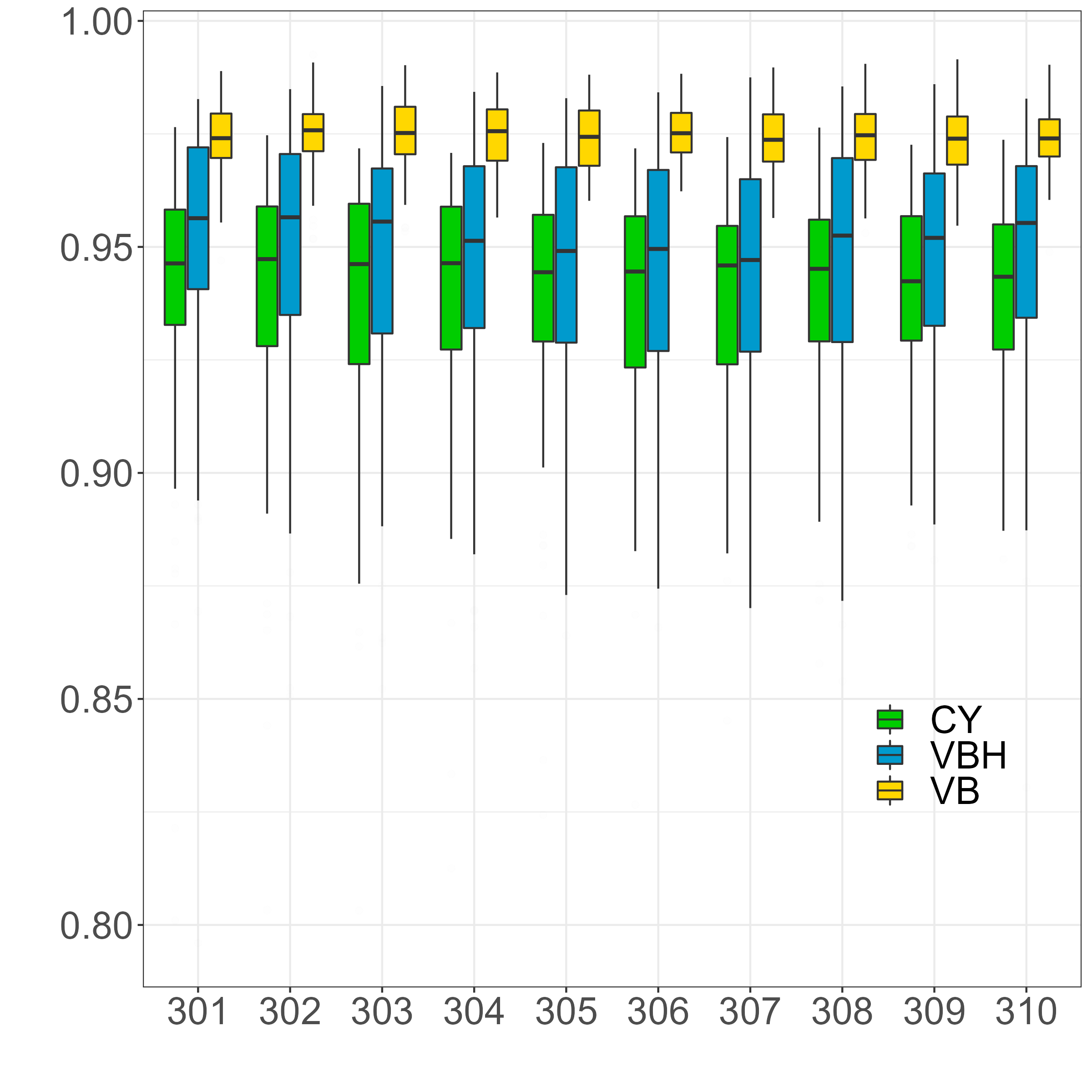
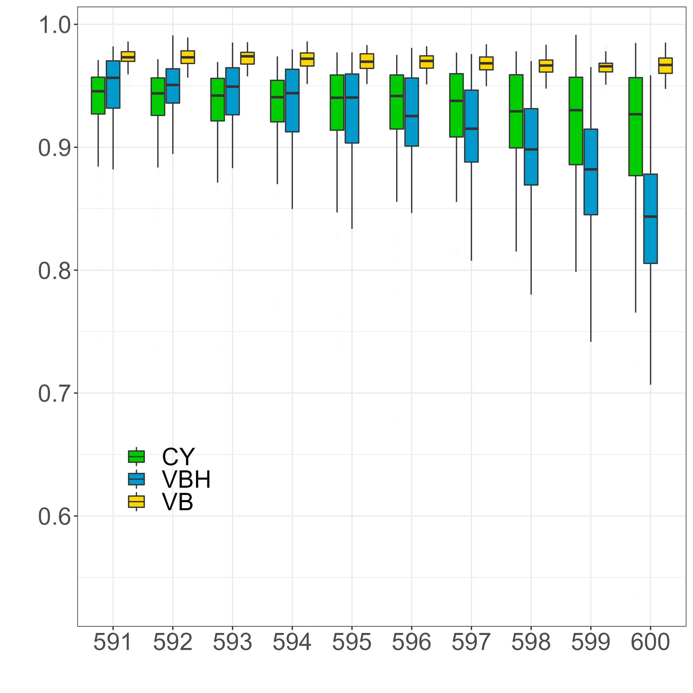
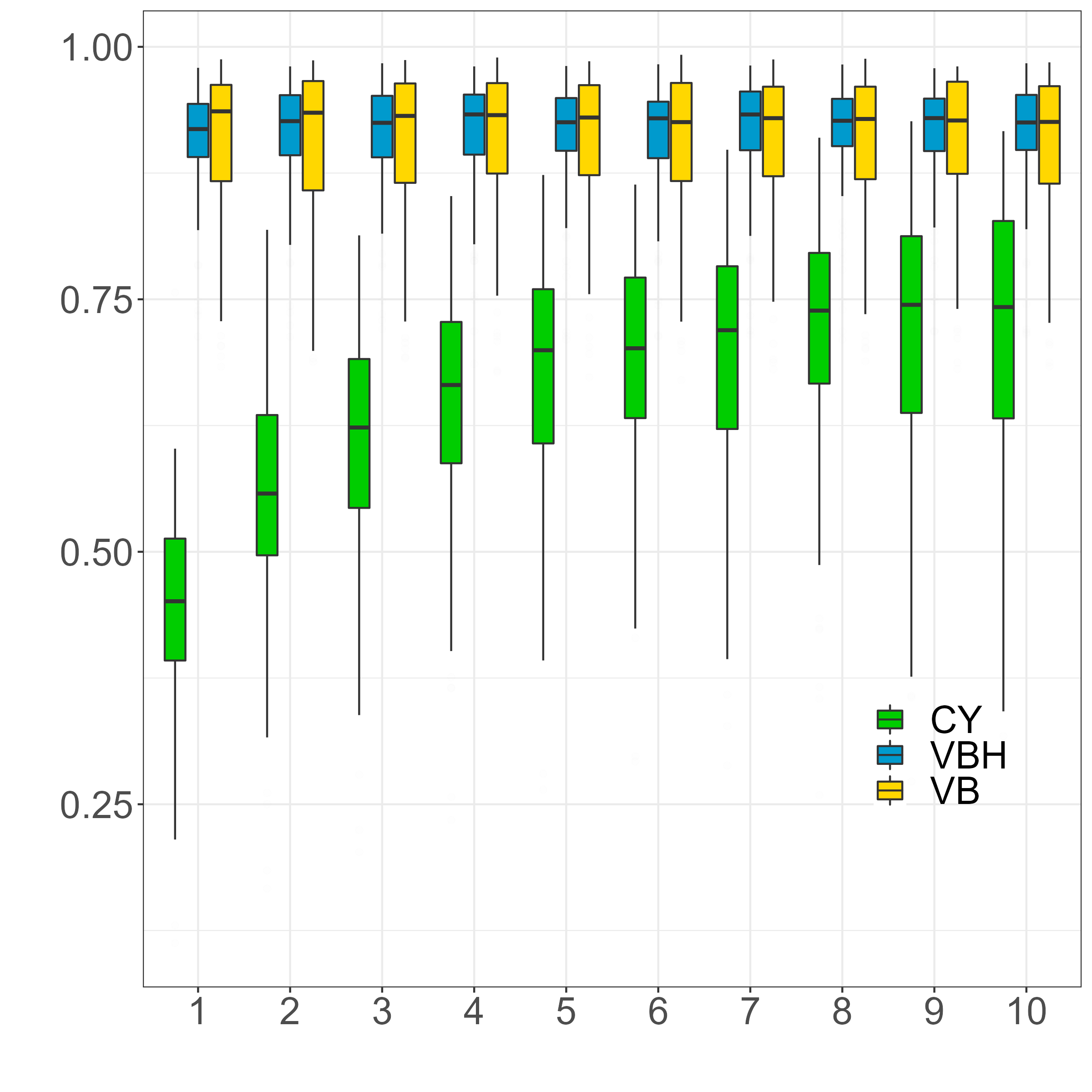
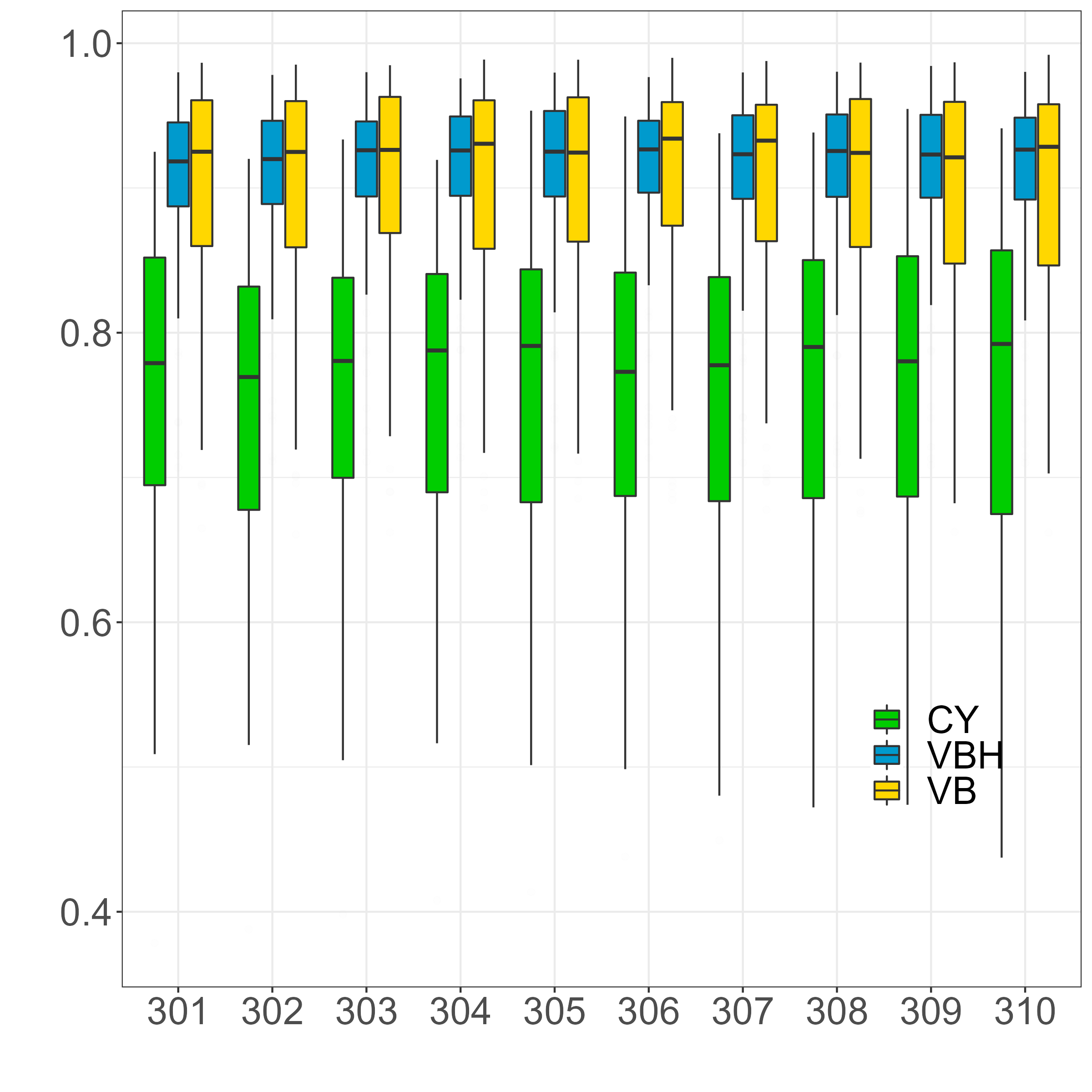
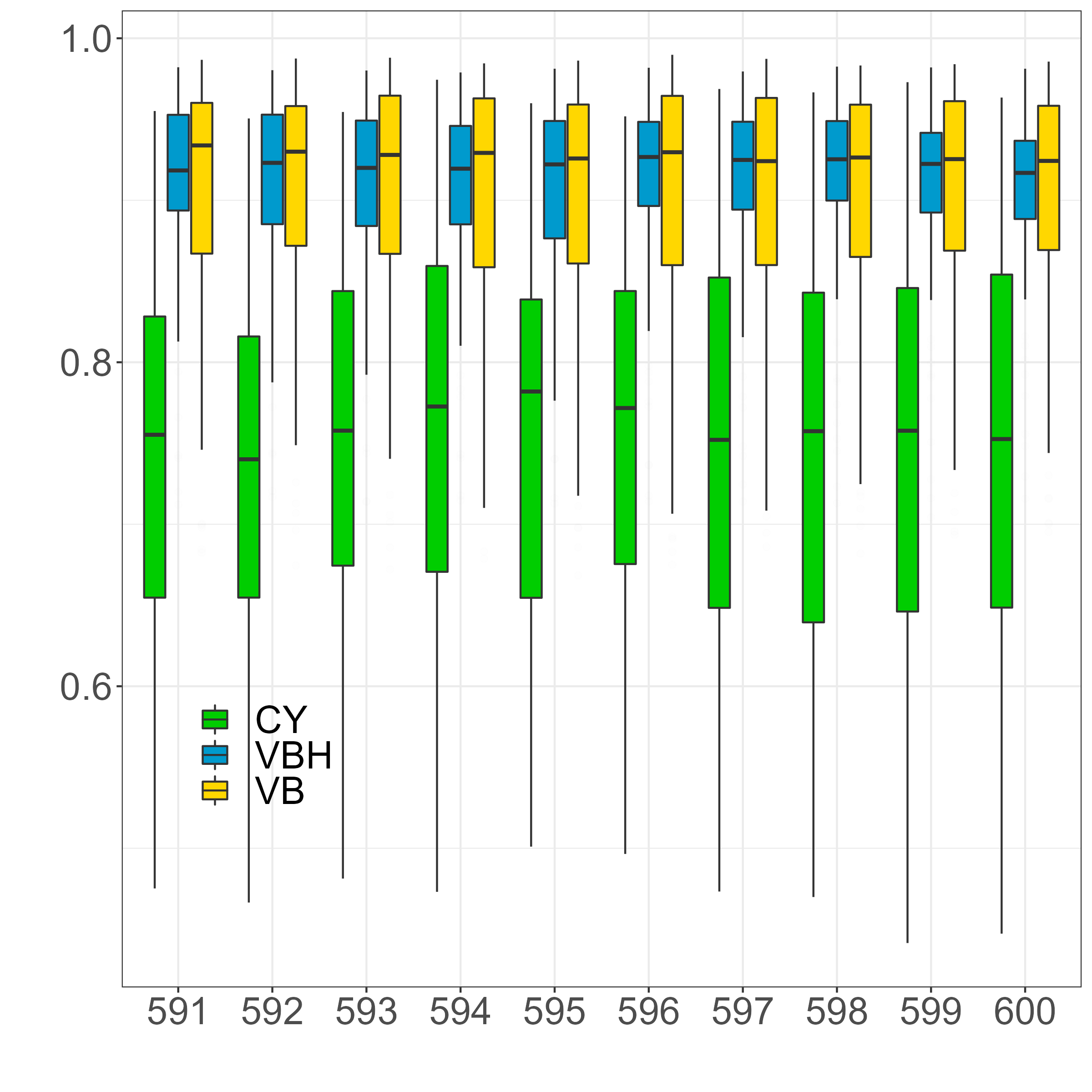
Online appendix for:
Smoothing volatility targeting

References

- Andersen and Sørensen (1996) T. G. Andersen and B. E. Sørensen. Gmm estimation of a stochastic volatility model: A monte carlo study. Journal of Business & Economic Statistics, 14(3):328–352, 1996.
- Bali (2000) T. G. Bali. Testing the empirical performance of stochastic volatility models of the short-term interest rate. Journal of Financial and Quantitative Analysis, 35(2):191–215, 2000.
- Bansal et al. (2010) R. Bansal, D. Kiku, and A. Yaron. Long run risks, the macroeconomy, and asset prices. American Economic Review, 100(2):542–46, 2010.
- Barroso and Detzel (2021) P. Barroso and A. Detzel. Do limits to arbitrage explain the benefits of volatility-managed portfolios? Journal of Financial Economics, 140(3):744–767, 2021.
- Barroso and Santa-Clara (2015) P. Barroso and P. Santa-Clara. Momentum has its moments. Journal of Financial Economics, 116(1):111–120, 2015.
- Bianchi et al. (2022) D. Bianchi, A. De Polis, and I. Petrella. Taming momentum crashes. Working paper, 2022.
- Bishop (2006) C. M. Bishop. Pattern Recognition and Machine Learning. Springer, 2006.
- Blei et al. (2017) D. M. Blei, A. Kucukelbir, and J. D. McAuliffe. Variational inference: A review for statisticians. Journal of the American Statistical Association, 112(518):859–877, 2017.
- Bongaerts et al. (2020) D. Bongaerts, X. Kang, and M. van Dijk. Conditional volatility targeting. Financial Analysts Journal, 76(4):54–71, 2020.
- Cederburg et al. (2020) S. Cederburg, M. S. O’Doherty, F. Wang, and X. S. Yan. On the performance of volatility-managed portfolios. Journal of Financial Economics, 138(1):95–117, 2020.
- Chan and Yu (2022) J. C. Chan and X. Yu. Fast and accurate variational inference for large bayesian vars with stochastic volatility. Journal of Economic Dynamics and Control, 143:104505, 2022.
- Chan et al. (2021) J. C. C. Chan, G. Koop, and X. Yu. Large Order-Invariant Bayesian VARs with Stochastic Volatility. Papers, arXiv.org, Nov. 2021.
- Corsi (2009) F. Corsi. A simple approximate long-memory model of realized volatility. Journal of Financial Econometrics, 7(2):174–196, 2009.
- Daniel and Moskowitz (2016) K. Daniel and T. J. Moskowitz. Momentum crashes. Journal of Financial Economics, 122(2):221–247, 2016.
- Durbin and Koopman (2000) J. Durbin and S. J. Koopman. Time series analysis of non-gaussian observations based on state space models from both classical and bayesian perspectives. Journal of the Royal Statistical Society. Series B (Statistical Methodology), 62(1):3–56, 2000.
- Fama and French (1996) E. F. Fama and K. R. French. Multifactor explanations of asset pricing anomalies. The journal of finance, 51(1):55–84, 1996.
- Fama and French (2015) E. F. Fama and K. R. French. A five-factor asset pricing model. Journal of financial economics, 116(1):1–22, 2015.
- Frazzini and Pedersen (2014) A. Frazzini and L. H. Pedersen. Betting against beta. Journal of financial economics, 111(1):1–25, 2014.
- Frazzini et al. (2012) A. Frazzini, R. Israel, and T. J. Moskowitz. Trading costs of asset pricing anomalies. Fama-Miller Working Paper, Chicago Booth Research Paper, (14-05), 2012.
- Gallant et al. (1997) A. Gallant, D. Hsieh, and G. Tauchen. Estimation of stochastic volatility models with diagnostics. Journal of Econometrics, 81(1):159–192, 1997.
- Gefang et al. (2019) D. Gefang, G. Koop, and A. Poon. Variational Bayesian inference in large Vector Autoregressions with hierarchical shrinkage. CAMA Working Paper, (2019-08), Jan. 2019.
- Ghysels et al. (1996) E. Ghysels, A. C. Harvey, and E. Renault. 5 stochastic volatility. In Statistical Methods in Finance, volume 14 of Handbook of Statistics, pages 119–191. Elsevier, 1996.
- Gibbons et al. (1989) M. R. Gibbons, S. A. Ross, and J. Shanken. A test of the efficiency of a given portfolio. Econometrica: Journal of the Econometric Society, pages 1121–1152, 1989.
- Gunawan et al. (2021) D. Gunawan, R. Kohn, and D. Nott. Variational bayes approximation of factor stochastic volatility models. International Journal of Forecasting, 37(4):1355–1375, 2021.
- Han (2006) Y. Han. Asset allocation with a high dimensional latent factor stochastic volatility model. The Review of Financial Studies, 19(1):237–271, 2006.
- Hansen et al. (2008) L. P. Hansen, J. C. Heaton, and N. Li. Consumption strikes back? measuring long-run risk. Journal of Political economy, 116(2):260–302, 2008.
- Hansen and Lunde (2005) P. R. Hansen and A. Lunde. A forecast comparison of volatility models: does anything beat a garch (1, 1)? Journal of applied econometrics, 20(7):873–889, 2005.
- Harvey et al. (1994) A. Harvey, E. Ruiz, and N. Shephard. Multivariate Stochastic Variance Models. The Review of Economic Studies, 61(2):247–264, 04 1994.
- Harvey et al. (2018) C. R. Harvey, E. Hoyle, R. Korgaonkar, S. Rattray, M. Sargaison, and O. Van Hemert. The impact of volatility targeting. The Journal of Portfolio Management, 45(1):14–33, 2018.
- Hinton and Van Camp (1993) G. Hinton and D. Van Camp. Keeping neural networks simple by minimizing the description length of the weights. In in Proc. of the 6th Ann. ACM Conf. on Computational Learning Theory. Citeseer, 1993.
- Hosszejni and Kastner (2021) D. Hosszejni and G. Kastner. Modeling univariate and multivariate stochastic volatility in R with stochvol and factorstochvol. Journal of Statistical Software, 100(12):1–34, 2021.
- Hou et al. (2015) K. Hou, C. Xue, and L. Zhang. Digesting anomalies: An investment approach. The Review of Financial Studies, 28(3):650–705, 2015.
- Jacquier et al. (2002) E. Jacquier, N. G. Polson, and P. E. Rossi. Bayesian analysis of stochastic volatility models. volume 20, pages 69–87. 2002. Twentieth anniversary commemorative issue.
- Jacquier et al. (2004) E. Jacquier, N. G. Polson, and P. E. Rossi. Bayesian analysis of stochastic volatility models with fat-tails and correlated errors. J. Econometrics, 122(1):185–212, 2004.
- Jegadeesh and Titman (1993) N. Jegadeesh and S. Titman. Returns to buying winners and selling losers: Implications for stock market efficiency. The Journal of finance, 48(1):65–91, 1993.
- Jensen et al. (2022) T. I. Jensen, B. T. Kelly, and L. H. Pedersen. Is there a replication crisis in finance? Journal of Finance, (Forthcoming), 2022.
- Jobson and Korkie (1981) J. D. Jobson and B. M. Korkie. Performance hypothesis testing with the sharpe and treynor measures. Journal of Finance, pages 889–908, 1981.
- Jordan et al. (1999) M. I. Jordan, Z. Ghahramani, T. S. Jaakkola, and L. K. Saul. An introduction to variational methods for graphical models. Machine learning, 37(2):183–233, 1999.
- Kim et al. (1998) S. Kim, N. Shephard, and S. Chib. Stochastic volatility: Likelihood inference and comparison with arch models. The Review of Economic Studies, 65(3):361–393, 1998.
- Koop and Korobilis (2020) G. Koop and D. Korobilis. Bayesian dynamic variable selection in high dimensions, 2020.
- Ledoit and Wolf (2008) O. Ledoit and M. Wolf. Robust performance hypothesis testing with the sharpe ratio. Journal of Empirical Finance, 15(5):850–859, 2008.
- Liu et al. (2019) F. Liu, X. Tang, and G. Zhou. Volatility-managed portfolio: does it really work? The Journal of Portfolio Management, 46(1):38–51, 2019.
- Melino and Turnbull (1990) A. Melino and S. M. Turnbull. Pricing foreign currency options with stochastic volatility. Journal of Econometrics, 45(1):239–265, 1990.
- Moreira and Muir (2017) A. Moreira and T. Muir. Volatility-managed portfolios. The Journal of Finance, 72(4):1611–1644, 2017.
- Ormerod and Wand (2010) J. T. Ormerod and M. P. Wand. Explaining variational approximations. The American Statistician, 64(2):140–153, 2010.
- Parisi (1988) G. Parisi. Statistical field theory, volume 66 of Frontiers in Physics. Benjamin/Cummings Publishing Co., Inc., Advanced Book Program, Reading, MA, 1988. With a foreword by David Pines.
- Patton and Weller (2020) A. J. Patton and B. M. Weller. What you see is not what you get: The costs of trading market anomalies. Journal of Financial Economics, 137(2):515–549, 2020.
- Rohde and Wand (2016) D. Rohde and M. P. Wand. Semiparametric mean field variational bayes: General principles and numerical issues. Journal of Machine Learning Research, 17(172):1–47, 2016.
- Rue and Held (2005) H. v. Rue and L. Held. Gaussian Markov random fields, volume 104 of Monographs on Statistics and Applied Probability. Chapman & Hall/CRC, Boca Raton, FL, 2005. Theory and applications.
- Ruiz (1994) E. Ruiz. Quasi-maximum likelihood estimation of stochastic volatility models. Journal of Econometrics, 63(1):289–306, 1994.
- Rustagi (1976) J. S. Rustagi. Variational methods in statistics. Academic Press [Harcourt Brace Jovanovich, Publishers], New York-London, 1976. Mathematics in Science and Engineering, Vol. 121.
- Sakurai (1994) J. J. Sakurai. Modern quantum mechanics; rev. ed. Addison-Wesley, Reading, MA, 1994.
- Schorfheide et al. (2018) F. Schorfheide, D. Song, and A. Yaron. Identifying long-run risks: A bayesian mixed-frequency approach. Econometrica, 86(2):617–654, 2018.
- Shephard (2020) N. Shephard. Statistical aspects of arch and stochastic volatility. In Time series models, pages 1–67. Chapman and Hall/CRC, 2020.
- Shephard and Pitt (2004) N. Shephard and M. K. Pitt. Erratum: “Likelihood analysis of non-Gaussian measurement time series” [Biometrika 84 (1997), no. 3, 653–667; mr1603940]. Biometrika, 91(1):249–250, 2004.
- Taylor (1994) S. J. Taylor. Modeling stochastic volatility: A review and comparative study. Mathematical finance, 4(2):183–204, 1994.
- Wand and Ormerod (2011) M. P. Wand and J. T. Ormerod. Penalized wavelets: embedding wavelets into semiparametric regression. Electron. J. Stat., 5:1654–1717, 2011.
- Wang and Yan (2021) F. Wang and X. S. Yan. Downside risk and the performance of volatility-managed portfolios. Journal of Banking & Finance, 131:106198, 2021.
- Yu (2005) J. Yu. On leverage in a stochastic volatility model. Journal of Econometrics, 127(2):165–178, 2005.