Stochastic thermodynamics of opinion dynamics

Abstract

We show that models of opinion formation and dissemination in a community of individuals can be framed within stochastic thermodynamics from which we can build a nonequilibrium thermodynamics of opinion dynamics. This is accomplished by decomposing the original transition rate that defines an opinion model into two or more transition rates, each representing the contact with heat reservoirs at different temperatures, and postulating an energy function. As the temperatures are distinct, heat fluxes are present even at the stationary state and linked to the production of entropy, the fundamental quantity that characterizes nonequilibrium states. We apply the present framework to a generic-vote model including the majority-vote model in a square lattice and in a cubic lattice. The fluxes and the rate of entropy production are calculated by numerical simulation and by the use of a pair approximation.

I Introduction

Opinion dynamics helbing1995 ; castellano2009 deals with the time evolution of the number of individuals in each of the various groups that a community is divided by reason of the opinion of the individuals concerning a given subject. The opinion of an individual changes with time under the influence of other individuals or by the influence of an external agent. The repeated action of these influences leads to a collective behavior of the individuals in relation to the opinions, which is the phenomenon to be explained by the opinion models. The modeling can be accomplished by expressing these influences in terms of rules that govern the opinion dynamics.

There are various possibilities of setting up opinion models according to the way one represents the opinion martins2008 ; jedrzejewski2019 . In view of the contingent character of the influences, we consider models with dynamics rules that have a stochastic nature. A way of representing the stochastic nature of the opinion dynamics is to consider it to be a continuous time Markovian process liggett1985 ; liggett1999 ; tome2015L defined on a space of opinions. This means to say that opinion models are defined once we are given the rates of the transition from an opinion state of the whole community to other possible opinion states.

Here we focus on models with a discrete space of opinions in which individuals, or agents, are located in space at sites whose collection forms a lattice of sites. To each individual, or to each site, one associates an opinion variable, understood as a random variable, that takes certain discrete numerical values, each corresponding to a certain opinion regarding the issue being discussed. The equation that governs the time evolution of the opinion probability is the master equation which is set up from the transition rates.

Many models fall within this framework. We mention the voter model clifford1973 ; holley1975 in which at each time step an individual takes the opinion of one of its neighbors chosen at random. The noise voter model, or linear Glauber model, which we call simply linear model, is a modification of the voter model such that the individual takes the opinion of the chosen neighbor with a certain probability and the opposite opinion with the complementary probability scheucher1988 ; krapivsky1992 ; granovsky1995 ; oliveira2003 . The original voter model was generalized to the case where the individual takes the opinion of two or more neighbors chosen randomly as long as they have a common opinion castellano2009a ; nyczka2012 . In the Sznajd model a pair of neighboring individuals with the same opinions convince all its neighbors to their opinion sznajd2000 . The voter model was generalized to the case in which each individual adopts three opinions, for instance, leftist, centrist and rightist vazquez2003 .

The majority-vote model oliveira1992 is based on a majority rule. An individual takes the opinion of the majority of its neighbor with a certain probability and the opposite opinion with the complementary probability. If there is a tie, the individual takes either opinion with equal probability. This model displays a critical phase transition from a disordered to an ordered state that belongs to the universality class of the Ising model, in spite of being a non-equilibrium model in the sense that its transition rate lacks detailed balance. It was originally defined in the square lattice but was applied to other regular lattices acunalara2012 ; acunalara2014 ; sastre2016 ; chatelain2022 as well as to small world lattices campos2003 , to random graphs pereira2005 ; lima2005 , and to complete graphs fronczak2017 . When inertia is incorporated to the majority-vote model, it exhibits a discontinuous phase transition chen2017 ; harunari2017 ; encinas2018 . A version of the majority-vote model with three states was also conceived brunstein1999 .

A generic-vote vote model with two states has been considered with the restriction that the change of opinion of an individual depends only on the sum of the opinions in a neighborhood oliveira1993 . In a square lattice this model has two parameters. Depending on the relation between these parameters, the generic-vote model reduces to the voter model, the linear model and the majority model. In general the transition rates do not obey detailed balance and the generic-vote model is a nonequilibrium model. However, for a special relation between the two parameters, it reduces to the Glauber model glauber1963 ; suzuki1968 .

The Glauber model is distinct from the other models described above in the sense that its transition rate obeys detailed balance from which follows that the stationary probability distribution is the Gibbs probability distribution, which is proportional to $e^{-\beta E}$, where $E$ is the energy function. It describes a system in thermodynamic equilibrium at a temperature inversely proportional to $\beta$. For the Glauber model, $E$ is the Ising energy function and the model defined by the equilibrium Gibbs probability distribution is known as the Ising model and can be interpreted as an opinion model with two states. In fact, such an interpretation was put forward as a sociological model and the two ordered states displayed by the Ising model were interpreted as the polarizations of opinions found in society weidlich1971 .

A similar interpretation was given to the Ising model with an approach that was supplemented by a thermodynamic basis galam1982 ; galam1991 . Accordingly, the free energy associated to the Ising model was interpreted as the dissatisfaction function and the principle of minimum free energy as a principle of minimum dissatisfaction. The energy function of the Ising model was interpreted as measure of the degree of convergence or divergence, that is, of agreement or conflict. Although these interpretations are appealing, they refer to equilibrium thermodynamics and cannot be extended to include the models presented above, which cannot be found in thermodynamic equilibrium as they do not obey detailed balance.

The statistical mechanics that has been used as the framework to opinion dynamics castellano2009 , which encompasses the master equation as the central evolution equation, emphasizes the probabilistic aspects but lacks a thermodynamics perspective as it makes no reference to energy nor to entropy, the two main concepts of thermodynamics, and much less to their relationship.

To circumvent these problems, we propose a framework to the models of opinion dynamics based on stochastic thermodynamics tome2010 ; esposito2012 ; seifert2012 ; vandebroeck2013 ; tome2015 , which is capable of describing systems out of thermodynamics equilibrium as well as system in thermodynamic equilibrium. The stochastic thermodynamics is appropriate for systems described by a master equation and can be understood as an enlargement of the statistical mechanics for systems out of thermodynamic equilibrium. This approach provides in addition an expression for the production of entropy, a keystone quantity that characterizes systems out of thermodynamic equilibrium.

The central and crucial idea that we use in the analysis of the models for opinion dynamics rests on the decomposition of the transition rate into several mutually exclusive transition rates. Each of these transition rates describes the contact with a heat reservoir at a certain temperature. The whole transition rate describes thus the contact with various heat reservoirs at distinct temperatures. As the temperatures are different, the transition rate does not obey detailed balance, and as a consequence, in the stationary state the system will not be found in thermodynamic equilibrium. It is worth pointing out that the idea of using heat reservoir at distinct temperatures is not new and has been used before. However, the reference to a heat reservoir was usually nominal and lacks the crucial Clausius relation between entropy, heat and reservoir temperature.

II Decomposition of the transition rates

We consider a community of individuals, each holding an opinion concerning a particular issue. The individuals are immobile and are located at the sites of a lattice. To properly describe the opinion of the whole community, we attach to each site an opinion variable $\sigma_{i}$ that takes one of several possible numerical values, each associated to an opinion concerning the issue at hand.

The opinion state, which is the collection of the opinions of the individuals, is denoted by $\sigma$. As time goes by, the opinion state changes according to a stochastic process. The rate at which the state changes from $\sigma$ to $\sigma^{\prime}$ is denoted by $W(\sigma^{\prime},\sigma$), which is the central quantity that defined a model of opinion dynamics. The probability $P(\sigma,t)$ of finding the whole community in a given opinion $\sigma$ at time $t$ obeys the master equation

$$\frac{d}{dt}P(\sigma)=\sum_{\sigma^{\prime}}\{W(\sigma,\sigma^{\prime})P(\sigma^{\prime})-W(\sigma^{\prime},\sigma)P(\sigma)\}.$$ (1)

The transition rate $W$ is decomposed into a certain number of transition rates $W_{\ell}$,

$$W(\sigma,\sigma^{\prime})=\sum_{\ell}W_{\ell}(\sigma,\sigma^{\prime}),$$ (2)

each holding the following property. Given $\sigma$ and $\sigma^{\prime}$, and if $W_{k}(\sigma,\sigma^{\prime})$ is nonzero then $W_{\ell}(\sigma,\sigma^{\prime})$ will vanish necessarily for $\ell\neq k$. The possible pairs of configuration $(\sigma,\sigma^{\prime})$ are partitioned into a certain number of mutually exclusive subsets, and one associates to each subset $\ell$ a transition rate $W_{\ell}(\sigma,\sigma)$ meaning that this transition vanishes if $(\sigma,\sigma^{\prime})$ does not belong to the subset $\ell$.

Another property of the rate $W_{\ell}$ is its association to an energy function. To express this property one starts by postulating an energy function $E(\sigma)$, which may be called the opinion function. Then the transition rate is set up in such a way that

$$\frac{W_{\ell}(\sigma^{\prime},\sigma)}{W_{\ell}(\sigma,\sigma^{\prime})}=e^{-[E(\sigma^{\prime})-E(\sigma)]/\theta_{\ell}},$$ (3)

where $\theta_{\ell}$ is a parameter. We remark that this property is possible if the process described by the rate $W_{\ell}$ has it reverse, or in other terms, if $W_{\ell}(\sigma^{\prime},\sigma)$ is nonzero so is $W_{\ell}(\sigma,\sigma^{\prime})$.

Let us suppose that the whole transition rate $W$ is composed by just one transition of the type (3). Then it will hold the property

$$\frac{W(\sigma^{\prime},\sigma)}{W(\sigma,\sigma^{\prime})}=e^{-[E(\sigma^{\prime})-E(\sigma)]/\theta}.$$ (4)

If we define the probability distribution

$$P_{0}(\sigma)=\frac{1}{Z}e^{-E(\sigma)/\theta},$$ (5)

we see that $P_{0}$ is the stationary solution of the master equation, which can be verified by the use of the property (4) which is the detailed balance condition. The distribution (5) is the Gibbs distribution which describes a system in thermodynamic equilibrium at a temperature $\theta$.

The whole transition rate $W$ that fulfills the detailed balance condition (4) can also be understood as the one appropriate to describe a system in contact with a heat reservoir at a temperature $\theta$. When $W$ is a sum of terms $W_{\ell}$, the detailed balance condition is not satisfied. At first sight the property (3) seems to be the detailed balance condition but it is not because $\theta_{\ell}$ in (3) is distinct for distinct $\ell$. However, we may interpret $W$ as describing a system in contact with several heat reservoir each being at a given temperature $\theta_{\ell}$. In the long run, when the steady state is reached, the system will not be found in the equilibrium state since the detailed balance is not satisfied, unless all temperatures are the same.

III Stochastic thermodynamics

III.1 General

The time derivative of the average energy $U=\langle E(\sigma)\rangle$ is obtained by multiplying the master equation (1) by $E(\sigma)$ and summing in $\sigma$. The result is

$$\frac{dU}{dt}=\Phi,$$ (6)

$$\Phi=\sum_{\ell}\Phi_{\ell},$$ (7)

$$\Phi_{\ell}=\sum_{\sigma\sigma^{\prime}}[E(\sigma^{\prime})-E(\sigma)]W_{\ell}(\sigma^{\prime},\sigma)P(\sigma).$$ (8)

The quantity $\Phi_{\ell}$ is understood as the flux of energy from the $\ell$-th heat reservoir to the system, and $\Phi$ is the total flux of energy from the reservoirs to the system.

The entropy of the system is defined by

$$S=-\sum_{\sigma}P(\sigma)\ln P(\sigma),$$ (9)

and depends on time. Its time derivative can be written by the use of the master equation (1) in the following form

$$\frac{dS}{dt}=\Pi-\Psi,$$ (10)

$$\Pi=\sum_{\ell}\Pi_{\ell},\qquad\Psi=\sum_{\ell}\Psi_{\ell},$$ (11)

where

$$\Pi_{\ell}=\frac{1}{2}\sum_{\sigma\sigma^{\prime}}\{W_{\ell}(\sigma,\sigma^{\prime})P(\sigma^{\prime}-W_{\ell}(\sigma^{\prime},\sigma)P(\sigma)\}\times$$

$$\times\ln\frac{W_{\ell}(\sigma,\sigma^{\prime})P(\sigma^{\prime})}{W_{\ell}(\sigma^{\prime},\sigma)P(\sigma)},$$ (12)

$$\Psi_{\ell}=\sum_{\sigma\sigma^{\prime}}W_{\ell}(\sigma^{\prime},\sigma)P(\sigma)\ln\frac{W_{\ell}(\sigma^{\prime},\sigma)}{W_{\ell}(\sigma,\sigma^{\prime})}.$$ (13)

The quantity $\Pi_{\ell}$ is the rate of the entropy production due to process $\ell$ and is a nonnegative quantity, and $\Pi$ is the total rate of entropy production. The quantity $\Psi_{\ell}$ is interpreted as the flux of entropy from the system to the reservoir $\ell$, and $\Psi$ is the total flux of entropy from the system to the reservoirs.

Next we use the property (3) to write the flux of entropy $\Psi_{\ell}$ in the form

$$\Psi_{\ell}=-\frac{1}{\theta_{\ell}}\sum_{\sigma\sigma^{\prime}}W_{\ell}(\sigma^{\prime},\sigma)P(\sigma)[E(\sigma^{\prime})-E(\sigma)].$$ (14)

Comparing this expression with (8), we reach the following relation between the flux of entropy and the flux of energy related to the reservoir $\ell$,

$$\Psi_{\ell}=-\frac{\Phi_{\ell}}{\theta_{\ell}}.$$ (15)

It is worth making the following comment concerning the stationary state. In this state $dU/dt=0$ and $dS/dt=0$, from which follows that

$$\sum_{\ell}\Phi_{\ell}=0,$$ (16)

and hence

$$\Pi=-\sum_{\ell}\frac{\Phi_{\ell}}{\theta_{\ell}}.$$ (17)

Although the sum of all fluxes of energy vanishes in the stationary state it does not mean that the sum on the right-hand side of (17) will vanish. This happens because the temperature are distinct from each other. Thus there is a continuous production of entropy and the system is out of thermodynamic equilibrium. The equilibrium will be reached if all temperatures are the same in which case the right-hand side of (17) vanishes. In this case the production of entropy vanishes and the system will be found in equilibrium.

A special type of transition rate could also be included in the decomposition (2) of $W(\sigma,\sigma^{\prime})$. This type of transition rate, which we label by $\ell=0$ is the one such that $W_{0}(\sigma,\sigma^{\prime})=W_{0}(\sigma^{\prime},\sigma)$. The corresponding contribution to the production of entropy is

$$\Pi_{0}=\frac{1}{2}\sum_{\sigma\sigma^{\prime}}W_{0}(\sigma,\sigma^{\prime})\{P(\sigma^{\prime})-P(\sigma)\}\ln\frac{P(\sigma^{\prime})}{P(\sigma)},$$ (18)

but the corresponding contribution to the flux of entropy vanishes. We assume that the variation in energy associated to this special type of transition rate vanishes, $E(\sigma^{\prime})=E(\sigma)$, which is consistent with the relation (4). Thus, the contribution to the flux of energy also vanishes.

The relation (15), which is a fundamental result coming out of the present approach, is identified as the essential and central relation of thermodynamics introduced by Clausius. However, the Clausius relation connects the entropy to the heat flux and not to the energy flux. To conform with Clausius we proceed as follows. The energy function $E(\sigma)$ that we have postulated and which appears in the definition (3) of the transition rates $W_{\ell}$ is replaced by the function $H(\sigma)$, which is $E(\sigma)$, understood as the internal energy, subtracted from the potential energy $L(\sigma)$ due to external forces, that is, $H=E-L$.

The time evolution of $U=\langle E\rangle$ is given by equations (6), (7), and (8), and that of $\langle L\rangle$ is given by

$$\frac{d\langle L\rangle}{dt}=\Phi^{\rm ext}=\sum_{\ell}\Phi_{\ell}^{\rm ext},$$ (19)

$$\Phi_{\ell}^{\rm ext}=\sum_{\sigma\sigma^{\prime}}[L(\sigma^{\prime})-L(\sigma)]W_{\ell}(\sigma^{\prime},\sigma)P(\sigma).$$ (20)

Using the same reasoning above we conclude that the entropy flux $\Psi_{\ell}$ from the system to the reservoir $\ell$ is now given by

$$\Psi_{\ell}=-\frac{\Phi_{\ell}^{\rm q}}{\theta_{\ell}},$$ (21)

where

$$\Phi_{\ell}^{\rm q}=\Phi_{\ell}-\Phi_{\ell}^{\rm ext}.$$ (22)

Writing $\Phi_{\ell}=\Phi_{\ell}^{\rm q}+\Phi_{\ell}^{\rm ext}$ we see that this equation can be understood as the conservation of energy and $\Phi_{\ell}^{\rm q}$ as the flux of heat. The first term is the variation of energy of the system and the last is the variation of the external potential per unit time, or power. From now on we treat the cases such that $L$ can be set to zero and the flux of heat is identified as the flux of energy.

III.2 One-site transitions

We consider here models such that at each time step just one individual changes its opinion. The individuals are located at the sites of a lattice and we suppose that each individual holds an opinion pro or against a particular issue. The opinion variable $\sigma_{i}$ then takes two values which we choose to be $+1$ or $-1$ according to whether the individual at the site $i$ of the lattice is pro or against the issue at hand, respectively. Thus the dynamics is defined by the transition rate $w_{i}(\sigma)$ that the individual at $i$ changes its opinion from the present to the opposite opinion, that is, from $\sigma_{i}$ to $-\sigma_{i}$, and the master equation reads

$$\frac{d}{dt}P(\sigma)=\sum_{i}\{w_{i}(\sigma^{i})P(\sigma^{i})-w_{i}(\sigma)P(\sigma)\},$$ (23)

where $\sigma^{i}$ stands for the state obtained from $\sigma$ by changing $\sigma_{i}$ to $-\sigma_{i}$. The one-site transition rate is decomposed in the form

$$w_{i}(\sigma)=\sum_{\ell}w_{\ell i}(\sigma),$$ (24)

where $w_{\ell i}$ holds the property

$$\frac{w_{\ell i}(\sigma)}{w_{\ell i}(\sigma^{i})}=e^{-[E(\sigma^{i})-E(\sigma)]/\theta_{\ell}},$$ (25)

where $E(\sigma)$ is the postulated energy. The transition rates $w_{\ell i}(\sigma)$ holds the property mentioned just below the equation (2). That is, if $\sigma$ is a state such that $w_{ki}(\sigma)$ is nonzero than $w_{\ell i}(\sigma)$ will vanish for $\ell\neq k$.

The time variation of the average energy $U$ is given by (6) and (7), where now the energy flux from the reservoir $\ell$ reads

$$\Phi_{\ell}=\sum_{\sigma}\sum_{i}[E(\sigma^{i})-E(\sigma)]w_{\ell i}(\sigma)P(\sigma),$$ (26)

which can be written as an average

$$\Phi_{\ell}=\sum_{i}\langle[E(\sigma^{i})-E(\sigma)]w_{\ell i}(\sigma)\rangle,$$ (27)

and can thus be obtained from numerical simulations.

The time variation of the entropy is given by (10) and (11), where now the rate of entropy production due to the process $\ell$ is

$$\Pi_{\ell}=\frac{1}{2}\sum_{\sigma}\sum_{i}\{w_{\ell i}(\sigma^{i})P(\sigma^{i})-w_{\ell i}(\sigma)P(\sigma)\}\times$$

$$\times\ln\frac{w_{\ell i}(\sigma^{i})P(\sigma^{i})}{w_{\ell i}(\sigma)P(\sigma)},$$ (28)

and is a nonnegative quantity, and the flux of entropy $\Psi_{\ell}$ from the system to the reservoir $\ell$ is

$$\Psi_{\ell}=\sum_{\sigma}\sum_{i}w_{\ell i}(\sigma)P(\sigma)\ln\frac{w_{\ell i}(\sigma)}{w_{\ell i}(\sigma^{i})}.$$ (29)

Using the relation (25) we reach again the result (15), namely, $\Psi_{\ell}=-\Phi_{\ell}/\theta_{\ell}$. We remark that the $\Psi_{\ell}$ given by (29) can be written as the following average

$$\Psi_{\ell}=\sum_{i}\left\langle w_{\ell i}(\sigma)\ln\frac{w_{\ell i}(\sigma)}{w_{\ell i}(\sigma^{i})}\right\rangle.$$ (30)

IV Contact with one heat reservoir

A transition rate $w_{i}$ that leads to the Gibbs equilibrium probability distribution

$$P_{0}(\sigma)=\frac{1}{Z}e^{E(\sigma)/\theta}$$ (31)

can be constructed by the use of the detailed balance condition

$$\frac{w_{i}(\sigma)}{w_{i}(\sigma^{i})}=\frac{P_{0}(\sigma^{i})}{P_{0}(\sigma)}=e^{-[E(\sigma^{i})-E(\sigma)]/\theta}.$$ (32)

The most general form of $w_{i}$ satisfying the detailed balance condition is

$$w_{i}(\sigma)=k_{i}(\sigma)e^{E(\sigma)/\theta},$$ (33)

where $k_{i}(\sigma^{i})=k_{i}(\sigma)$, that is, $k_{i}(\sigma)$ does not depend on $\sigma_{i}$. If we define $\alpha_{i}(\sigma_{i})$ by

$$\alpha_{i}(\sigma)=k_{i}(\sigma)[e^{E(\sigma^{i})/\theta}+e^{E(\sigma)/\theta}],$$ (34)

we see that the transition rate can be written in the form

$$w_{i}(\sigma)=\frac{1}{2}\alpha_{i}(\sigma)[1-\tanh\frac{E(\sigma^{i})-E(\sigma)}{2\theta}],$$ (35)

where $\alpha_{i}(\sigma)$, as happens to $k_{i}(\sigma)$, does not depend on $\sigma_{i}$, that is, $\alpha_{i}(\sigma^{i})=\alpha_{i}(\sigma)$, which is also a general form of $w_{i}(\sigma)$ satisfying the detailed balance condition. Since this transition leads to the equilibrium Gibbs distribution, we may interpret it as describing the contact with a heat reservoir at a temperature $\theta$.

If the energy function is

$$E(\sigma)=-\sum_{(ij)}\sigma_{i}\sigma_{j},$$ (36)

where the summation is over all nearest neighbor pairs of sites, then

$$w_{i}(\sigma)=\frac{1}{2}\alpha_{i}(\sigma)[1-\sigma_{i}\tanh\frac{1}{\theta}\sum_{\delta}\sigma_{i+\delta}],$$ (37)

where the summation is over the nearest neighbor sites of site $i$.

When $\alpha_{i}$ does not depend on $\sigma$, that is, when it is a constant,

$$w_{i}(\sigma)=\frac{\alpha}{2}[1-\sigma_{i}\tanh\frac{1}{\theta}\sum_{\delta}\sigma_{i+\delta}],$$ (38)

and it is called Glauber transition rate because Glauber used it to describe the dynamics of the one-dimensional Ising model. In this case the expression (38) can be simplified and reads

$$w_{i}(\sigma)=\frac{\alpha}{2}[1-\frac{\gamma}{2}\sigma_{i}(\sigma_{i-1}+\sigma_{i+1})],$$ (39)

where $\gamma=\tanh 2/\theta$. In fact, this is the originalexpression used by Glauber in 1963 glauber1963 . That given by (38) was introduced later on by Suzuki and Kubo in 1968 suzuki1968 .

V Generic-vote model

V.1 General

We apply the results of the previous section to the generic-vote model introduced in reference oliveira1993 . In this model the change of opinion of an individual depends only on the sum of the opinions of the nearest neighbor individuals. We consider here a square lattice in which case the number of nearest neighbors is four, and the possible values of the sum are $4,2,0,-2,-4$. The rates at which the opinion changes are given in table 1.

We will consider the transition rate with reference to a certain site labeled 0. In addition, the four nearest neighbor of site 0 are labeled 1, 2, 3, and 4, which are respectively on the right, above, left and below the site zero. The transition rate related to the site zero is assumed to be of the form

$$w=\frac{1}{2}(1-\sigma_{0}f),$$ (40)

where $f$ is a function of the opinion variables associated to the four nearest neighbor of site 0. Notice that we are dropping the site index of $w$ and $f$. For the generic-vote model $f$ is given by oliveira1993

$$f=s(a+b\sigma_{1}\sigma_{2}\sigma_{3}\sigma_{4}),$$ (41)

$$s=\sigma_{1}+\sigma_{2}+\sigma_{3}+\sigma_{4},$$ (42)

where $a$ and $b$ are parameters related to $p$ and $q$ by

$$a=\frac{1}{8}(p+2q),\qquad b=\frac{1}{8}(p-2q),$$ (43)

or $p=4(a+b)$ and $q=2(a-b)$.

Replacing these relations in (41), we write

$$f=q\,\xi_{1}+p\,\xi_{2},$$ (44)

where

$$\xi_{1}=\frac{s}{4}(1-\sigma_{1}\sigma_{2}\sigma_{3}\sigma_{4}),$$ (45)

$$\xi_{2}=\frac{s}{8}(1+\sigma_{1}\sigma_{2}\sigma_{3}\sigma_{4}).$$ (46)

Notice $\xi_{1}$ takes the values $1$ and $-1$ for $s$ equal to $2$ and $-2$, and the value zero otherwise; and that $\xi_{2}$ takes the values $1$ and $-1$ for $s$ equal to $4$ and $-4$, and the value zero otherwise.

The transition rate $w$ is invariant under the inversion of all variables $\sigma_{i}$, which amounts to say that $f$ changes sign under the inversion transformation. The expression (41) is the most generic form for $f$ obeying this invariance oliveira1993 . As shown in table 1, the transition rate $w$ for the generic-vote model depends only on the four nearest neighbor variables only through their sum $s$.

Table 1: Transition rates of the generic-vote model in a square lattice. The transition rates depend on the possible values $4,2,0,-2,-4$ of the sum of the opinion variables of the neighboring individuals.

$\sigma_{0}\to-\sigma_{0}$	4	2	0	-2	-4
$1\to-1$	$\frac{1}{2}(1-p)$	$\frac{1}{2}(1-q)$	$\frac{1}{2}$	$\frac{1}{2}(1+q)$	$\frac{1}{2}(1+p)$
$-1\to 1$	$\frac{1}{2}(1+p)$	$\frac{1}{2}(1+q)$	$\frac{1}{2}$	$\frac{1}{2}(1-q)$	$\frac{1}{2}(1-p)$

The decomposition of the transition rate $w$ is carried out by postulating an energy function, which we choose to be that given by (36). The transition rate is written as the sum of three transition rates,

$$w=g_{0}+g_{1}+g_{2},$$ (47)

two of them being of the type (37),

$$g_{1}=\frac{1}{2}\alpha_{1}[1-\sigma_{0}\tanh\frac{s}{\theta_{1}}],$$ (48)

$$g_{2}=\frac{1}{2}\alpha_{2}]1-\sigma_{0}\tanh\frac{s}{\theta_{2}}],$$ (49)

which describe the contact with heat reservoirs at temperatures $\theta_{1}$ and $\theta_{2}$, respectively. The third component $g_{0}$ is chosen not depend on $\sigma_{0}$ so that $g_{0}(\sigma^{i})=g_{0}(\sigma)$. We write $g_{0}=\alpha_{0}/2$.

The first process associated to the transition rate $g_{1}$, which describes the contact with the first reservoir at temperature $\theta_{1}$, occurs when $s=\pm 2$; and the second process associated to the transition rate $g_{2}$, which describes the contact with the second reservoir at temperature $\theta_{2}$, occurs when $s=\pm 4$; and we assume that the process labeled zero occurs when $s=0$. These assumptions are accomplished by setting $\alpha_{1}$ equal to $1$ for $s\pm 2$, and zero otherwise; $\alpha_{2}$ equal to $1$ for $s\pm 4$, and zero otherwise; and $\alpha_{0}$ equal to $1$ for $s=0$, and zero otherwise.

If we consider the transition $1\to-1$ and $s=2$, then $w=g_{1}=(1-\tanh 2/\theta_{1})$ which, according to table 1, must be equal to $(1-q)/2$, and we conclude that

$$q=\tanh\frac{2}{\theta_{1}}.$$ (50)

Analogously, if we consider the transition $1\to 1$ and $s=4$, then $w=g_{2}=(1-\tanh 4/\theta_{2})$ which, according to table 1, must be equal to $(1-p)/2$, and we conclude that

$$p=\tanh\frac{4}{\theta_{2}}.$$ (51)

The relations of the parameters $p$ and $q$ with the temperatures $\theta_{1}$ and $\theta_{2}$, given by (50) and (51), can also be obtained as follows. We start by writing the following equivalent forms of $g_{1}$ and $g_{2}$,

$$g_{1}=\frac{1}{2}\alpha_{1}[1-\sigma_{0}\frac{s}{2}\tanh\frac{2}{\theta_{1}}],$$ (52)

$$g_{2}=\frac{1}{2}\alpha_{2}[1-\sigma_{0}\frac{s}{4}\tanh\frac{4}{\theta_{2}}],$$ (53)

and by replacing them in (47). The result for $w$ is of the form (40) with $f$ is given by

$$f=\alpha_{1}\frac{s}{2}\tanh\frac{2}{\theta_{1}}+\alpha_{2}\frac{s}{4}\tanh\frac{4}{\theta_{2}},$$ (54)

where we used the relation $\alpha_{0}+\alpha_{1}+\alpha_{2}=1$. Taking into account that $\alpha_{1}s=2\xi_{1}$ and $\alpha_{2}s=4\xi_{2}$, we reach the result

$$f=\xi_{1}\tanh\frac{2}{\theta_{1}}+\xi_{2}\tanh\frac{4}{\theta_{2}},$$ (55)

which compared with (44) leads us to the results (50) and (51).

V.2 Specific models

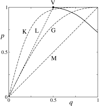
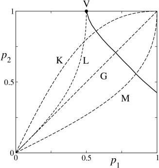
Depending on the values of the parameters $q$ and $p$, several models are particular cases of the generic-vote model. They correspond to a certain relation between $q$ and $p$, and thus described by lines in the diagrams of figures 1 and 2. The majority-vote model oliveira1992 is defined by the transition rate

$$w_{\rm M}=\frac{1}{2}(1-\gamma\sigma_{0}{\cal S}),$$ (56)

where $\gamma$ is a parameter and ${\cal S}(s)$ is a function of $s$ that takes the values $-1,0,+1$, when $s<0$, $s=0$, $s>0$, respectively. We see that the transition rate $w$ reduces to the majority-vote transition rate when $p=q=\gamma$ or equivalently when $a=-3b=3\gamma/8$. The temperatures are related to $\gamma$ by

$$\theta_{1}=\frac{4}{\ln(1+\gamma)/(1-\gamma)},$$ (57)

and $\theta_{2}=2\theta_{1}$.

When $b=0$, the model reduces to the linear model oliveira2003 , defined by the transition rate

$$w_{\rm L}=\frac{1}{2}(1-a\sigma_{0}s).$$ (58)

In this case $p=2q=4a$, and

$$\theta_{1}=\frac{4}{\ln(1+2a)/(1-2a)},$$ (59)

$$\theta_{2}=\frac{8}{\ln(1+4a)/(1-4a)}.$$ (60)

Figure 1: Phase diagram of the generic-vote model in a square lattice in the plane $q=\tanh 2/\theta_{1}$ and $p=\tanh 4/\theta_{2}$. The dashed lines correspond to majority-vote (M) model, Glauber (G) model, model K, and linear (L) model. The small full circle (V) corresponds to the voter model. Below the line G, $\theta_{2}>\theta_{1}$, and above it $\theta_{2}<\theta_{1}$. Along the line G, $\theta_{2}=\theta_{1}$. The solid line is the critical line separating the ordered state, above the line, from the disordered state, below the line. The critical point of the models K, G, and M occur at $q_{c}=0.576(2)$ $q_{c}=\sqrt{2}/2$, and $q_{c}=0.850(2)$ oliveira1992 , respectively.

If $b=0$ and in addition $a=1/4$, then the model reduces to the voter model holley1975 , defined by the transition rate

$$w_{\rm V}=\frac{1}{2}(1-\frac{1}{4}\sigma_{0}s).$$ (61)

In this case $p=1$, and $q=1/2$, and

$$\theta_{1}=\frac{4}{\ln 3},$$ (62)

and $\theta_{2}\to 0$. The vanishing of $\theta_{1}$ is a consequence of the fact that when $s=\pm 4$, the reverse transition rate vanishes.

The Glauber transition rate is given by

$$w_{\rm G}=\frac{1}{2}(1-\sigma_{0}\tanh\frac{s}{\theta}),$$ (63)

and describes the contact of a system with energy function (36) with a reservoir at temperature $\theta$. Using the relation

$$\tanh\frac{s}{\theta}=\xi_{1}\tanh\frac{2}{\theta}+\xi_{2}\tanh\frac{4}{\theta},$$ (64)

it follows that the generic-vote transition rate reduces to the Glauber transition rate if $q=\tanh 2/\theta$ and $p=\tanh 4/\theta$, that is,

$$\theta_{1}=\theta_{2}=\theta.$$ (65)

From this relation between it follows that $p$ and $q$ are connected by

$$p=\frac{2q}{1+q^{2}}.$$ (66)

Figure 2: Same as figure 1 but in the plane $p_{1}=\tanh 2/\theta_{1}$ and $p_{2}=\tanh 2/\theta_{2}$.

As an example of a model whose fluxes of energy is the opposite of the majority vote model we define a model corresponding to a temperature $\theta_{2}$ smaller than $\theta_{1}$. We choose $\theta_{2}=\theta_{1}/2$, and call it model K. Using (50) and (51), the relation between $p$ and $q$ for model K is

$$p=\frac{4q(1+q^{2})}{1+6q^{2}+q^{4}}.$$ (67)

VI Fluxes of energy and entropy production

VI.1 Square lattice

There are two quantities that interest us here which are the fluxes of energy and the rate of entropy production in the stationary state. From the formula (27), we see that there is no flux of energy due to the zero process because in this case the energy $E$ remains the same. The energy fluxes per site due to the first and second processes are

$$\phi_{1}=2\langle\sigma_{0}sg_{1}\rangle,\qquad\phi_{2}=2\langle\sigma_{0}sg_{2}\rangle,$$ (68)

because $E(\sigma^{0})-E(\sigma)=2\sigma_{0}s$. In the stationary state the rate of entropy production per site is given by

$${\cal P}=-\frac{\phi_{1}}{\theta_{1}}-\frac{\phi_{2}}{\theta_{2}},$$ (69)

and taking into account that $\phi_{1}+\phi_{2}=0$, we may write

$${\cal P}=\phi_{2}\left(\frac{1}{\theta_{1}}-\frac{1}{\theta_{2}}\right).$$ (70)

Figure 3: Flux of energy $\phi_{2}$ from the second to the firs reservoir as a function of $q$ for the majority-vote model (M), for the linear model (L), and for the model K. For the Glauber model (G) the flux vanishes. The critical points of models M and K occur at the inflexion point and are indicated by small full circles. The triangle represents the flux of energy for the voter model. The results were obtained by numerical simulations on a square lattice with $100\times 100$ sites.

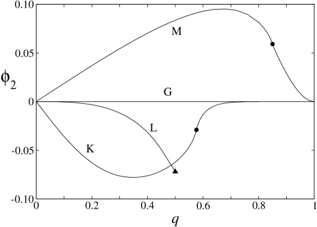
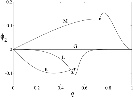
The quantity $\phi_{2}$ represents the flux of energy that traverses the system from the second to the first reservoir. Taken into account that ${\cal P}>0$ then if $\theta_{2}>\theta_{1}$ then $\phi_{2}>0$ and energy flows from the second to the first reservoir. This happens to the models with parameters $p$ and $q$ in the region below the line G of the diagrams of figures 1 and 2. Above this line $\theta_{2}<\theta_{1}$, and since ${\cal P}>0$, then $\phi_{2}<0$ and energy flows effectively from the first to the second reservoir as happens to model K and the linear model. Along the line G, the energy flux $\phi_{2}$ vanishes.

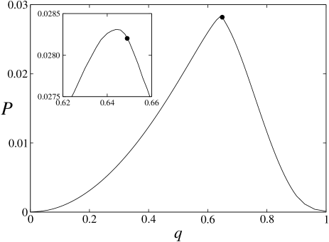
From equation (68), we see that the energy fluxes are averages and can thus be calculated from numerical simulations. We have simulated the majority-vote model, the model K and the linear model in a square lattice with sizes $100\times 100$ sites with periodic boundary conditions. The fluxes of energy as a function of $q$ are shown if figure 3. It is positive for the majority-vote model, and negative for the model K and for linear model as expected. From the flux of energy, the rate of the production of entropy is determined from equation (70) and is shown in figure 4. The entropy production of the majority-vote model in a square lattice has already been calculated in a direct manner by the use of equation (30) crochik2005 . This equation has also been used to calculate the production of entropy in other models and as a means of characterizing nonequilibrium phase transitions noa2019 .

Figure 4: Rate of entropy production ${\cal P}$ as a function of $q$ for the majority-vote model (M), for the linear model (L), and for the model K. The critical point of models M and K occur at the inflexion point and are indicated by small full circles. The curve L diverges at $q=0.5$. The results were obtained from the fluxes shown in figure 3 by the use of formula (70).

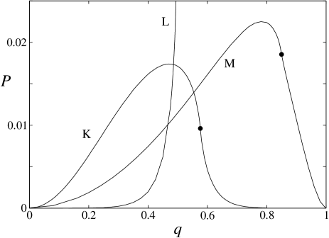
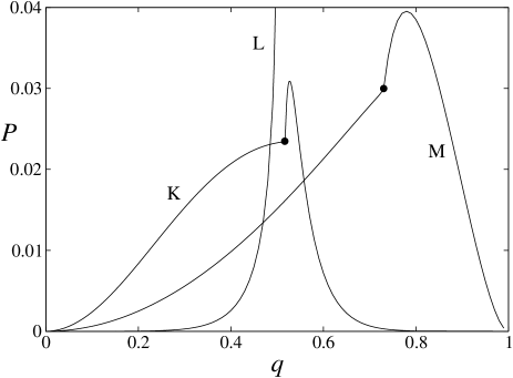
The generic-vote model is found to undergo a phase transition oliveira1993 from a disordered state characterized by $\langle\sigma_{i}\rangle=0$, occurring for small values of $q$ and $p$, to an ordered state characterized by $\langle\sigma_{i}\rangle\neq 0$, occurring at higher values of $q$ and $p$, as shown in figures 1 and 2. When one moves from inside the ordered state region to the transition line, $\langle\sigma_{i}\rangle$ vanishes continuously. The criticality behavior of the model is reflected as a singularity in $\phi$ and ${\cal P}$ at the inflexion points of these quantities which occur at $q_{c}=0.850(2)$ for the majority-vote model oliveira1992 and $q_{c}=0.576(2)$ for the model K. The linear model becomes critical at the voter point occurring at $q=0.5$. At this point, $\phi_{2}$ is finite but ${\cal P}$ diverges.

It should be pointed out that for finite lattices the slope at the inflexion point of the fluxes and the rate of entropy production is finite. As one increases the size of the lattice, the slope becomes greater and diverges in the thermodynamic limit, characterizing a true singularity crochik2005 . As we shall see below, the same is true for the model defined in a cubic lattice.

VI.2 Cubic lattice

The generic-vote model can also be defined in a cubic lattice. In this case it is necessary to introduce three heat reservoirs to describe appropriately the transition rates. The six nearest neighbor sites to a central site 0 are labeled $1,2,3,4,5,6$ and we denote by $s$ the sum $s=\sigma_{1}+\sigma_{2}+\sigma_{3}+\sigma_{4}+\sigma_{5}+\sigma_{6}$ and by $\theta_{1}$, $\theta_{2}$, and $\theta_{3}$ the temperatures of the three reservoirs. The transition rate is

$$w=g_{0}+g_{1}+g_{2}+g_{3},$$ (71)

where $g_{0}=\alpha_{0}/2$, and

$$g_{1}=\frac{1}{2}(\alpha_{1}-\sigma_{0}\xi_{1}q),$$ (72)

$$g_{2}=\frac{1}{2}(\alpha_{2}-\sigma_{0}\xi_{2}p),$$ (73)

$$g_{3}=\frac{1}{2}(\alpha_{3}-\sigma_{0}\xi_{3}r),$$ (74)

where $q=\tanh 2/\theta_{1}$, $p=\tanh 4/\theta_{2}$, $r=\tanh 6/\theta_{3}$; and $\alpha_{0}=1$ when $s=0$, and zero otherwise; $\alpha_{1}=1$ when $s=\pm 2$, and zero otherwise; $\alpha_{2}=1$ when $s=\pm 4$, and zero otherwise; and $\alpha_{3}=1$ when $s=\pm 6$, and zero otherwise; whereas $\xi_{1}$ takes the values $1$ and $-1$ for $s$ equal to $2$ and $-2$, and zero otherwise; $\xi_{2}$ takes the values $1$ and $-1$ for $s$ equal to $4$ and $-4$, and zero otherwise; and $\xi_{3}$ takes the values $1$ and $-1$ for $s$ equal to $6$ and $-6$, and zero otherwise.

Figure 5: Fluxes of energy $\phi_{1}$, $\phi_{2}$, and $\phi_{3}$ as functions of $q$ for the majority-vote model in a cubic lattice. The critical transition point occurs at the inflexion point of the curves and are indicated by small full circles. The results were obtained by numerical simulations on a cubic lattice with $20\times 20\times 20$ sites.

The fluxes of energy per site are given by

$$\phi_{\ell}=2\langle\sigma_{0}sg_{\ell}\rangle,$$ (75)

and the rate of entropy production per site is given by

$${\cal P}=-\frac{\phi_{1}}{\theta_{1}}-\frac{\phi_{2}}{\theta_{2}}-\frac{\phi_{3}}{\theta_{3}}.$$ (76)

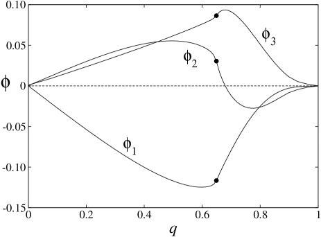
The generic-vote model on the cubic line, defined by the transition rates above, reduces to the majority-vote model on the cubic lattice when $p=q=r$ which implies that the temperature are related by $\theta_{1}=\theta_{2}/2=\theta_{3}/3$. We have simulated the majority-vote model on a cubic lattice with $20\times 20\times 20$ sites with periodic boundary conditions. We determined the three energy fluxes $\phi_{1}$, $\phi_{2}$, and $\phi_{3}$ in the stationary state and they are shown in figure 5. Within the statistical errors we verified that $\phi_{1}+\phi_{2}+\phi_{3}=0$. The model displays a critical phase transition that occurs at the inflexion points of the fluxes which we found to be $q_{c}=0.649(2)$ which is in agreement with previous calculation on the location of the critical point, $q_{c}=0.6474(2)$ acunalara2012 .

We have also determined the rate of entropy production ${\cal P}$, which is shown in figure 6 and we see that it is in fact positive although the three fluxes do not have the same sign.

Figure 6: Rate of entropy production ${\cal P}$ as a function of $q$ for the majority-vote model in a cubic lattice. The critical transition point is indicated by a small full circle and does not occur at the maximum of the curve as can be seen in the inset. The results were obtained from the fluxes shown in figure 5 by the use of formula (76).

VII Pair approximation

We solve the master equation (23) by means of a pair approximation tome1989 . Denoting by $P(\sigma_{1},\sigma_{2},\sigma_{3},\sigma_{4}|\sigma_{0})$ the conditional probability associated to the four neighboring sites of site zero, the pair approximation consists in writing

$$P(\sigma_{1},\sigma_{2},\sigma_{3},\sigma_{4}|\sigma_{0})=\prod_{i}P(\sigma_{i}|\sigma_{0}),$$ (77)

where $P(\sigma_{i}|\sigma_{0})=P(\sigma_{i},\sigma_{0})/P(\sigma_{0})$. The pair probability is parametrized as follows

$$P(\sigma_{i},\sigma_{0})=\frac{1}{4}[1+m(\sigma_{0}+\sigma_{i})+r\sigma_{0}\sigma_{i}],$$ (78)

where $m=\langle\sigma_{0}\rangle=\langle\sigma_{i}\rangle$ and $r=\langle\sigma_{0}\sigma_{i}\rangle$. From this expression,

$$P(\sigma_{0})=\frac{1}{2}(1+m\sigma_{0}).$$ (79)

Figure 7: Flux of energy $\phi_{2}$ from the second to the first reservoir as a function of $q$ for the majority-vote model (M), for the linear model (L), and for the model K. For the Glauber model (G) the flux vanishes. The critical points of models V and K occur at the kink of the curves and are indicated by small full circles. The triangle represents the flux of energy for the voter model. The results were obtained from the pair approximation on a square lattice.

It is convenient to define the quantities

$$A_{n}=\frac{(m+r)^{n}}{(1+m)^{n-1}},\qquad B_{n}=\frac{(m-r)^{n}}{(1-m)^{n-1}}.$$ (80)

In terms of these quantities we get

$$\langle\sigma_{0}\sigma_{1}\ldots\sigma_{n}\rangle=\frac{1}{2}(A_{n}-B_{n}),$$ (81)

$$\langle\sigma_{1}\ldots\sigma_{n}\rangle=\frac{1}{2}(A_{n}+B_{n}).$$ (82)

To determine the time evolution of $m$, we multiply the the master equation (23) by $\sigma_{0}$ and sum in the variables $\sigma_{i}$ after employing (77) on the right-hand side of (23). The result is

$$\frac{dm}{dt}=-m+4am+2b(A_{3}+B_{3}).$$ (83)

Similarly, we find the time evolution of $r$, which is

$$\frac{dr}{dt}=-2r+2a+3(a+b)(A_{2}+B_{2})+b(A_{4}+B_{4}).$$ (84)

Figure 8: Rate of entropy production ${\cal P}$ as a function of $q$ for the majority-vote model (M), for the linear model (L), and for the model K. For the linear model, ${\cal P}$ diverges at $q=1/2$. The critical points of models V and K occur at the kink of the curves and are indicated by small full circles. The results were obtained from the fluxes of figure 7 by the use of formula (70).

A stationary solution of these equations is $m=0$ and $r$ the root of the equation

$$r=a+3(a+b)r^{2}+br^{4},$$ (85)

and corresponds to the disordered state. A stability analysis is obtained by the expansion of the right-hand side of (83) in powers of $m$. The solution becomes unstable when the coefficient of $m$ vanishes, that is, when

$$4a+12br^{2}-8br^{3}=1.$$ (86)

By inspection we see that the solution of equations (85) and (86) is $r=1/3$ and $27a+7b=27/4$, or

$$17p+20q=27,$$ (87)

which describes the critical line in the plane $p,q$ that separates the disordered and ordered states. The critical line ends on the voter point $p=1$ and $q=1/2$. The critical point of the majority vote model occurs when $p=q=27/37$, the Glauber model when $q=3/5$ and $p=15/17$, and the model K when $q=0.517246$ and $p=0.979710$.

Another solution corresponds to the ordered state for which $m\neq 0$. The values of $m$ and $r$ for this solution can be obtained by solving the equations (83) and (84), what we did numerically.

To determine the energy fluxes we observe that they can be written in terms of correlations of two and for sites. Using (51) and (50), we may write $g_{1}$ and $g_{2}$, given by (52) and (53), as

$$g_{1}=\frac{1}{2}(\alpha_{1}-\sigma_{0}\xi_{1}q),$$ (88)

$$g_{2}=\frac{1}{2}(\alpha_{2}-\sigma_{0}\xi_{2}p).$$ (89)

We then replace these results in

$$\phi=\frac{1}{2}(\phi_{2}-\phi_{1})=\langle\sigma_{0}s(g_{2}-g_{1})\rangle.$$ (90)

to find

$$\phi=\frac{1}{2}\langle[\sigma_{0}(4\xi_{1}-2\xi_{2})-s(\xi_{2}p-\xi_{1}q)]\rangle,$$ (91)

where we used the relations $\alpha_{1}s=2\xi_{1}$ and $\alpha_{2}s=4\xi_{2}$. Replacing the expression of $\xi_{1}$ and $\xi_{2}$ given by equations (45) and (46) in this equation we find

$$\phi=\frac{1}{2}\langle\sigma_{0}s\sigma_{1}\sigma_{2}\sigma_{3}\sigma_{4}-s^{2}(b+a\sigma_{1}\sigma_{2}\sigma_{3}\sigma_{4})\rangle.$$ (92)

It is then straightforward to write $\phi$ in the form

$$\phi=2\langle\sigma_{0}\sigma_{1}\sigma_{2}\sigma_{3}\rangle-2b-2a\langle\sigma_{1}\sigma_{2}\sigma_{3}\sigma_{4}\rangle$$

$$-4(a+b)\langle\sigma_{1}\sigma_{2}\rangle-2(a+b)\langle\sigma_{1}\sigma_{3}\rangle,$$ (93)

where the sites 1 and 3, and 2 and 4 are opposite in relation to the central site 0. This is accomplished by using symmetric operations that leave a square lattice invariant.

From the stationary solutions for $m$ and $r$, calculated numerically, we have determined the values of $\langle\sigma_{0}\sigma_{1}\sigma_{2}\sigma_{3}\rangle$, $\langle\sigma_{1}\sigma_{2}\sigma_{3}\sigma_{4}\rangle$, $\langle\sigma_{1}\sigma_{2}\rangle$, and $\langle\sigma_{1}\sigma_{3}\rangle$ by the use of (81) and (82). From these values we have determined $\phi$ by (93). In the stationary state $\phi_{1}=-\phi_{2}$ so that $\phi_{2}=\phi$. The flux of energy $\phi_{2}$ is shown in figure 7 as a function of $q$ for the majority model, the model K and for the linear model. From $\phi_{2}$, we have determined the rate of entropy production by (70), which is shown in figure 8 as a function of $q$ for the majority model, the model K and for the linear model.

For the Glauber model, our numerical calculations obtained from the pair approximation show that the flux $\phi_{2}$ vanishes for any value of $q$. This result shows that this approximation is capable of preserving the detailed balance condition for the models that hold this property as happens with the Glauber model.

VIII Conclusion

We have shown that the models of opinion dynamics can be framed within the stochastic thermodynamics from which we may construct a nonequilibrium thermodynamics of opinion dynamics. To this end we postulated an energy function, which we have called the opinion function, which is absent in the original definition of a model as it is defined by the transition rate. From the energy function, we define by the use of formula (3) the various components of the transition rate that defines the model that we wish to study. Each component is understood as describing the contact with heat reservoirs at distinct temperatures. As the temperatures are different from one another, the system will be in a nonequilibrium state at the stationary state, which is one of the main feature of the opinion dynamics.

Given a model, we face the problem of finding the energy function. Here, we have circumvented this problem by postulating a certain energy function and then determining the possible transition rates that follows from that energy function. In the present case we adopted the Ising energy function with nearest neighbor interactions, given by (36) and then proved that it leads to the generic-vote model by using (25).

The idea of using heat reservoirs at distinct temperatures or effective temperatures to define transition rates leading to nonequilibrium steady states is not new and has been used before, for instance, in the analysis of the generic-vote model drouffe1999 . The reference to heat reservoirs or to effective temperatures is usually nominal. Here we justify this idea by presenting a systematic approach in which a given state of the system is associated to just one of the heat reservoirs, with a transition rate describing the contact with the heat reservoir being given by (3). Our approach leads to the significant Clausius relation (15) between flux of entropy, flux of heat and temperature of the reservoir, that characterizes thermodynamically the contact of a system with a heat reservoir.

We have applied the approach developed here to nonequilibrium lattice models with two states that include the majority-vote model in the square lattice and the cubic lattice. In the square lattice it suffices to use two heat reservoirs but in the cubic lattice it is necessary three heat reservoirs to set up the transition rates. We have determined the fluxes of energy from each reservoir from which we determined the rate of entropy flux. The critical phase transition from a disordered to an ordered state that takes place in the models analyzed here is reflected in the fluxes and the production of entropy as a singularity occurring at the inflexion point of these quantities. We have also used a pair approximation in which case the singularity is characterized by a kink.

The approach proposed here is general and can be applied to stochastic models as long as their dynamic rules can be expressed by transition rates that can be decomposed into transition rates describing each one of them the contact with a heat reservoir.

References

- (1) D. Helbing, Quantitative Sociodynamics, (Springer, Berlin, 1995).
- (2) C. Castellano, S. Fortunato, and V. Loreto, Rev. Mod. Phys. 81, 591 (2009).
- (3) A. C. R. Martins, Int. J. Mod. Phys. C 19, 617 (2008).
- (4) A. Jȩdrzejewski and K. Sznajd-Weron, Comptes Rendus Physique 20, 244 (2019).
- (5) T. M. Liggett, Interacting Particle Systems (Springer, New York, 1985).
- (6) T. M. Liggett, Stochastic Interacting Systems: Contact, Voter, and Exclusion Processes (Spinger, Berlin, 1999).
- (7) T. Tomé and M. J. de Oliveira, Stochastic Dynamics and Irreversibility (Springer, Cham, 2015).
- (8) P. Clifford and A. Sudbury, Biometrika 60, 581 (1973).
- (9) R. A. Holley and T. M. Liggett, Annals of Probability 3, 643 (1975).
- (10) M. Scheucher and H. Spohn, J. Stat. Phys. 53, 279 (1988).
- (11) P. L. Krapivsky, Phys. Rev. A 54, 1067 (1992).
- (12) B. Granovsky and N. Madras, Stoch. Proc. Appl. 55, 23 (1995).
- (13) M. J. de Oliveira, Phys. Rev. E 67, 066101 (2003).
- (14) C. Castellano, M.A. Muñoz, and R. Pastor-Satorras, Phys. Rev. E 80, 041129 (2009).
- (15) P. Nyczka, K. Sznajd-Weron, and J. Cisło, Phys. Rev. E 86, 011105 (2012).
- (16) K. Sznajd-Weron and J. Sznajd, Int. J. Mod. Phys. 11, 1157 (2000).
- (17) F. Vazquez, P. L. Krapivsky, and S. Redner, J. Phys. A 36, L61 (2003).
- (18) M. J. de Oliveira, J. Stat. Phys. 66, 273 (1992).
- (19) Ana L. Acuña-Lara and F. Sastre, Phys. Rev. E 86, 041123 (2012).
- (20) Ana L. Acuña-Lara, F. Sastre, and J. R. Vargas-Arriola, Phys. Rev. E 89, 052109 (2014).
- (21) F. Sastre and M. Henkel, Physica A 444, 897 (2016).
- (22) C. Chatelain, ArXiv: 2211.00999
- (23) P. R. A. Campos, V. M. de Oliveira, and F. G. Brady Moreira, Phys. Rev. E 67, 026104 (2003).
- (24) L. F. C. Pereira and F. G. Brady Moreira, Phys. Rev. E 71, 016123 (2005)
- (25) F. W. S. Lima, U. L. Fulco, and R. N. Costa Filho, Phys. Rev. E 71, 036105 (2005).
- (26) A. Fronczak, P. Fronczak, Physical Review E 96, 012304 (2017).
- (27) H. Chen, C. Shen, H. Zhang, G. Li, Z. Hou, and J. Kurths, Phys. Rev. E 95, 042304 (2017).
- (28) P. E. Harunari, M. M. de Oliveira, and C. E. Fiore Physical Review E 96, 042305 (2017).
- (29) J. M. Encinas, P. E. Harunari, M. M. de Oliveira, and C. E. Fiore, Scientific Reports 8, 1 (2018).
- (30) A. Brunstein and T. Tomé, Phys. Rev. E 60, 3666 (1999).
- (31) M. J. de Oliveira, J. F. F. Mendes, and M. A. Santos, J. Phys. A 26, 2317 (1993).
- (32) R. J. Glauber, J. Math. Phys. 4, 294 (1963).
- (33) M. Suzuki and R Kubo, J. Phys. Soc. Japan 24, 51 (1968).
- (34) W. Weidlich, Br. J. Math. Statist. Psychol. 24, 251 (1971).
- (35) S. Galam, Y. Gefen, and Y. Shapir, Journal of Mathematical Sociology 9, 1 (1982).
- (36) S. Galam and S. Moscovici, European Journal of Social Psychology 21, 49 (1991).
- (37) T. Tomé and M. J. de Oliveira, Phys. Rev. E 82, 021120 (2010).
- (38) M. Esposito, Phys. Rev. E 85, 041125 (2012).
- (39) U. Seifert, Rep. Prog. Phys. 75, 126001 (2012).
- (40) C. Van de Broeck, in C. Bechinger, F. Sciortino, and P. Ziherl (eds.), Proceedings of the International School of Physics Enrico Fermi, Course 184, IOS, Amsterdam, 2013; p. 155.
- (41) T. Tomé and M. J. de Oliveira, Phys. Rev. E 91, 042140 (2015).
- (42) L. Crochik and T. Tomé, Phys. Rev. E 72, 057103 (2005).
- (43) C. E. F. Noa, P. E. Harunari, M. J. de Oliveira, and C. E. Fiore Phys. Rev. E 100, 012104 (2019).
- (44) T. Tomé and M. J. de Oliveira Phys. Rev. A 40, 6643 (1989).
- (45) J.-M. Drouffe and C. Godrèche J. Phys. A 32 249 (1999).