Setting the Scale Using Baryon Masses with Isospin-Breaking Corrections

Abstract

MITP-22-101, DESY-22-198

1 Introduction

We are in an era of precision lattice QCD, where contributions from QED and strong isospin-breaking can no longer be ignored in calculations of many phenomenologically relevant observables. An example where these contributions are of significant importance is in the lattice determination of the anomalous magnetic moment of the muon $(g-2)_{\mu}$. One of the largest uncertainties in any lattice determination of $(g-2)_{\mu}$ comes from the scale setting [1], and it is of great importance that the physical scale is determined with sufficient accuracy (i.e. below $1\%$), incorporating QED and isospin-breaking effects.

As lattice QCD ensembles are simpler to generate in the isosymmetric theory $\text{QCD}_{\text{iso}}$ than in full QCD+QED, many existing ensembles are isospin-symmetric. One method to incorporate isospin-breaking effects is based on their perturbative treatment on isosymmetric ensembles [2, 3]. The goal of our project is to employ this formalism to perform a precision calculation of the lattice scale for the $N_{f}=2+1$ CLS ensembles.

In refs. [4, 5], the lattice scale for the CLS ensembles was determined using a combination of pion and kaon decay constants. While the final result has a total error at the level of 1%, the incorporation of isospin-breaking corrections turns out to be conceptually quite difficult [6]. In this project, we investigate the prospects of precision scale setting using the masses of the lowest-lying baryon octet and decuplet, for which isospin-breaking effects are simpler to incorporate. In this contribution we present first preliminary results for our most promising candidates for the reference scale on two CLS ensembles, N451 and D450, with anti-periodic temporal boundary conditions.

We begin by giving an overview of our simulation setup and the isospin-breaking expansion of baryonic two-point functions in section 2. We then continue with an introduction of our fit strategy in section 3 and a discussion of the practical aspects and first insights of our analysis in section 4. Finally, a summary of the most important points and our plans for the next steps in this project are given in section 5.

2 Simulation Setup and Expansion in Isospin-Breaking Parameters

Our analysis makes use of the CLS $N_{f}=2+1$ ensembles [7] with $\mathcal{O}(a)$-improved Wilson fermions [8] and a tree-level Lüscher-Weisz gauge action [9]. Our choice of quark sources are SU(3)-covariantly Wuppertal-smeared [10] point sources. We apply APE smearing [11] to the gauge links. The smearing parameters were chosen such that they minimize the nucleon effective mass at an early time on the H105 ensemble and that the smearing radius as defined in [12] is approximately $0.5\text{\,}\mathrm{f}\mathrm{m}$.

The baryonic operators used for this project follow a construction introduced by the Lattice Hadron Physics Collaboration [13]. This construction yields a number of operators for each octet and decuplet baryon state, resulting in correlator matrices for each baryon. For a more detailed description of our implementation of these operators, we refer to [14].

For improved precision, we use all-mode-averaging [15, 16, 17] with 32 sloppy sources per gauge-configuration and one source for bias-correction on the ensembles discussed in section 4.

In order to determine baryon masses, we consider baryonic two-point functions of the form $C(t)=\expectationvalue{\mathcal{B}(t)\overline{\mathcal{B}}(0)}$ computed from zero-momentum projected baryonic creation and annihilation operators $\overline{\mathcal{B}}=\overline{B}\overline{\Psi}\overline{\Psi}\overline{\Psi}$ and $\mathcal{B}=B\Psi\Psi\Psi$, where $\overline{B}$ and $B$ encode the spinor, flavor, and color structure of the operators as well as their time-dependence. As we use isospin-symmetric gauge ensembles, we include isospin-breaking effects in terms of an expansion of full QCD+QED two-point functions about their counterparts in $\text{QCD}_{\text{iso}}$. This procedure was first introduced by the RM123 collaboration [2, 3] as an expansion in terms of the electromagnetic coupling $e$, the deviations $\Delta m_{u}$ and $\Delta m_{d}$ of the light quark masses from their isospin-symmetric counterpart $m_{ud}$ as well as a shift in the inverse strong gauge coupling $\Delta\beta$ and the strange quark mass $\Delta m_{s}$. In the following, we will collect these coefficients into a vector $\Delta\varepsilon$ which is to be understood as the difference of a vector $\varepsilon=(\beta,e^{2},m_{u},m_{d},m_{s})$ parameterizing QCD+QED and the corresponding vector $\varepsilon^{(0)}=(\beta,0,m_{ud},m_{ud},m_{s}^{(0)})$ parameterizing $\text{QCD}_{\text{iso}}$ and whose entries we denote by $\Delta\varepsilon_{i}$. Note that we explicitly assume $\Delta\beta=0$ throughout.

For baryonic correlation functions as defined above, this expansion takes the form

$$C^{\varepsilon}(t)= C^{\varepsilon^{(0)}}(t)+\sum_{f}\Delta m_{f}\partialderivative{C^{\varepsilon}(t)}{m_{f}}\evaluated{}_{\varepsilon=\varepsilon^{(0)}}+e^{2}\partialderivative{C^{\varepsilon}(t)}{e^{2}}\evaluated{}_{\varepsilon=\varepsilon^{(0)}},$$

where the superscripts $\varepsilon$ and $\varepsilon^{(0)}$ indicate that the correlation functions are computed in QCD+QED or $\text{QCD}_{\text{iso}}$ respectively. In a diagramatic representation, the above expansion can be written as

$$\expectationvalue{\vbox{\hbox{\includegraphics[width=79.6678pt]{plots/bar2pt}}}}^{\varepsilon}= \expectationvalue{\vbox{\hbox{\includegraphics[width=79.6678pt]{plots/bar2pt_0}}}}^{\varepsilon^{(0)}}+\sum_{f}\Delta m_{f}\expectationvalue{\vbox{\hbox{\includegraphics[width=79.6678pt]{plots/bar2pt_1_detf}}}}^{\varepsilon^{(0)}}$$

$$+e^{2}\expectationvalue{\vbox{\hbox{\includegraphics[width=79.6678pt]{plots/bar2pt_1_exch}}}+\vbox{\hbox{\includegraphics[width=79.6678pt]{plots/bar2pt_1_tad}}}+\vbox{\hbox{\includegraphics[width=79.6678pt]{plots/bar2pt_1_bow}}}}^{\varepsilon^{(0)}}$$

$$+\cdots$$

This expansion shows only those contributions which we consider in this study, i.e. only the quark-connected contributions. The complete first order in isospin-breaking parameters furthermore contains corrections in the sea-quark sector [3], which we do not include in our calculations. We do, however, compute diagrams containing a single photon vertex with an open-ended photon line which we can use later if we decide to include photon exchanges between valence and sea quarks. The correction terms are implemented using the method of sequential propagators.

3 Baryon Spectroscopy at Leading Order in Isospin-Breaking Corrections

The baryon masses are extracted from the two-point functions using the asymptotic description $C(t)=ce^{-mt}$ which holds for large time-separations $t$ between source and sink. Using a perturbative approach to incorporate isospin-breaking effects, the two-point functions must be expanded to the desired order to extract the corrections to the baryon masses. Expanding a general correlation function and its asymptotic form in terms of the isospin-breaking parameters $\Delta\varepsilon$ up to leading order via $X=X^{(0)}+\sum_{i}\Delta\varepsilon_{i}X_{i}^{(1)}+\mathcal{O}(\Delta\varepsilon^{2})$ where $X\in\{c,m,C\}$ and $X_{i}^{(1)}:=\partialderivative{X}{\varepsilon_{i}}\evaluated{}_{\varepsilon=\varepsilon^{(0)}}$, and matching the zeroth and first order, one finds

$$C^{(0)}(t)= c^{(0)}e^{-m^{(0)}t},$$

$$C_{i}^{(1)}(t)= \quantity(c_{i}^{(1)}-c^{(0)}m_{i}^{(1)}t)e^{-m^{(0)}t}.$$

From these expressions, the masses at zeroth and first order in $\Delta\varepsilon$ can be extracted as

$$\begin{aligned} m^{(0)}=&-\derivative{t}\log(C^{(0)}(t)),\\ m_{i}^{(1)}=&-\derivative{t}\frac{C_{i}^{(1)}(t)}{C^{(0)}(t)}.\end{aligned}$$ (1)

For our analysis we use the following discretizations for these expressions as definitions for the effective masses of the baryons:

$$\begin{aligned} (am_{\text{eff}})^{(0)}(t):=&\log(\frac{C^{(0)}(t)}{C^{(0)}(t+a)}),\\ (am_{\text{eff}})_{i}^{(1)}(t):=&\frac{C_{i}^{(1)}(t)}{C^{(0)}(t)}-\frac{C_{i}^{(1)}(t+a)}{C^{(0)}(t+a)}.\end{aligned}$$ (2)

The expressions in eq. 2 approach a plateau as $t\to\infty$. In practice, however, excited states affect the effective mass at early times. This would in principle not be much of a problem if there were little noise in the region where the excited state effects become negligible. However, since baryonic two-point functions suffer from signal-to-noise ratios growing exponentially with $t$ [18, 19], it is often difficult to determine the position of this region. Thus, to mitigate these deviations from a simple plateau, we include one excited state in addition to the ground state, in which case the correlation function takes the form

$$C_{2s}(t)=ce^{-mt}+c_{*}e^{-m_{*}t},$$ (3)

where $m$ is the ground state mass and $m_{*}$ is the mass of the first excitation. Inserting eq. 3 into eq. 1 one finds

$$(am)_{\text{eff}}^{(0)}(t)=\frac{am^{(0)}+\frac{c_{*}^{(0)}}{c^{(0)}}am_{*}^{(0)}e^{-\Delta M^{(0)}t}}{1+\frac{c_{*}^{(0)}}{c^{(0)}}e^{-\Delta M^{(0)}t}}$$ (4)

where $\Delta M^{(0)}=m_{*}^{(0)}-m^{(0)}$. Following Del Debbio et al. [20] we use a fit function obtained from eq. 4 by expansion in terms of $\frac{c_{*}^{(0)}}{c^{(0)}}e^{-\Delta M^{(0)}t}$:

$$(am)^{(0)}_{\text{eff}}(t)=am^{(0)}+\frac{c_{*}^{(0)}}{c^{(0)}}a\Delta M^{(0)}e^{-\Delta M^{(0)}t}=:am^{(0)}+\gamma e^{-\Delta M^{(0)}t}.$$ (5)

Performing the expansion in isospin-breaking parameters for the two-state ansatz (eq. 3) and plugging the result into the first order formula in eq. 1, one finds a similar fit function by expansion in terms of the same quantity as to obtain eq. 5:

$$(am)_{\text{eff}}^{(1)}=am^{(1)}+(\alpha-\beta t)e^{-\Delta M^{(0)}t},$$ (6)

where

$$\alpha= \gamma\quantity(\frac{\Delta M^{(1)}}{\Delta M^{(0)}}-\frac{c^{(1)}}{c^{(0)}}+\frac{c_{*}^{(1)}}{c_{*}^{(0)}}),$$

$$\beta= \gamma a\Delta M^{(1)},$$

$$\Delta M^{(k)}= m_{*}^{(k)}-m^{(k)}.$$

Notice that the exponent in eq. 6 is the same as that in eq. 5. This reduces the number of fit parameters in the first order fits as one can simply reuse the fit results for $\Delta M^{(0)}$ from the zeroth order fits.

For the fits designed to determine the isospin-symmetric contribution, an expansion in terms of $\frac{c_{*}^{(0)}}{c^{(0)}}e^{-\Delta M^{(0)}t}$ is not strictly necessary as the exact expression (eq. 4) is generally not more difficult to fit than the approximation and doesn’t introduce any further independent fit parameters. For the isospin breaking corrections, however, the exact expression has one more independent parameter and the mass correction $m^{(1)}$ cannot be extracted in a straightforward way compared to the expansion in eq. 6.

4 First Results

For this project, we have processed two ensembles (N451 at $m_{\pi}\approx$215\text{\,}\mathrm{M}\mathrm{e}\mathrm{V}$$ and D450 at $m_{\pi}\approx$290\text{\,}\mathrm{M}\mathrm{e}\mathrm{V}$$) with a lattice spacing of $a\approx$0.076\text{\,}\mathrm{f}\mathrm{m}$$ (determined in the isospin-symmetric theory [4] using combinations of the decay constants $f_{\pi}$, $f_{K}$, and the scale quantity $t_{0}$ derived from the Wilson flow [21]). Both of these ensembles have antiperiodic temporal boundary conditions with volumes of $128\times 48^{3}$ for N451 and $128\times 64^{3}$ for D450.

The analysis on these ensembles is based on the fit models described in section 3 with the two-point functions calculated as described in section 2. Our reasoning to study excited state effects in our data arise from the problem of identifying a plateau in noisy data, which requires that excited-state effects are sufficiently suppressed relative to the statistical fluctuations. In addition to giving a clearer picture as to where a plateau might start, a two-state fit often gives a more reliable estimate of the mass of the ground state than a single-state fit. Especially in fits to isospin-breaking corrections, where the extent of the plateau is not always clearly recognizable due to quickly growing uncertainties towards larger $t$, the determination of the asymptotic effective mass benefits from a consideration of excited states. We find that for many of our correlation functions, the behaviour of the effective mass indeed suggests a late plateau which starts in a region where the statistical noise is already quite large. Therefore, estimates based on a single exponential might introduce systematic uncertainties.

The two-state fits come in two kinds (see eqs. 5 and 6) both of which assume that the second excited state contribution is negligible in the chosen fit interval. Another approximation by Taylor expansion furthermore restricts the start of the fit interval to values where $\quantity(\frac{c_{*}^{(0)}}{c^{(0)}}e^{-\Delta M^{(0)}t})^{2}\ll 1$. The isospin-symmetric fits can be done using the exact formula eq. 4, however, the fit intervals are chosen such that eq. 5 is equally valid.

As the value for $\Delta M^{(0)}$ in eq. 6 is taken from the isospin-symmetric fit, the fit interval for the isospin-breaking corrections is chosen such that a zeroth-order fit with the same interval would result in a value for $\Delta M^{(0)}$ that is compatible with the one used for the isospin-symmetric fit.

Note that $\Delta M^{(0)}$ does not necessarily correspond to the mass difference between the ground state and the first excited state as corrections from higher excited states can in principle be absorbed by this fit value, especially if the fit interval starts at small values of $t$ where the statistical noise might be small enough for the effective mass to be sensitive to these corrections. Furthermore, the spectrum of excited states is, in general, too dense to be resolved in a single two-point-function. $\Delta M^{(0)}$ should therefore not be understood as a physical quantity but rather as a proxy to parameterize the curvature of the effective mass.

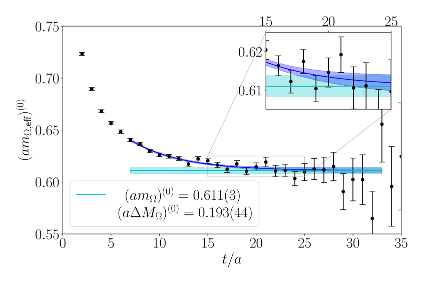
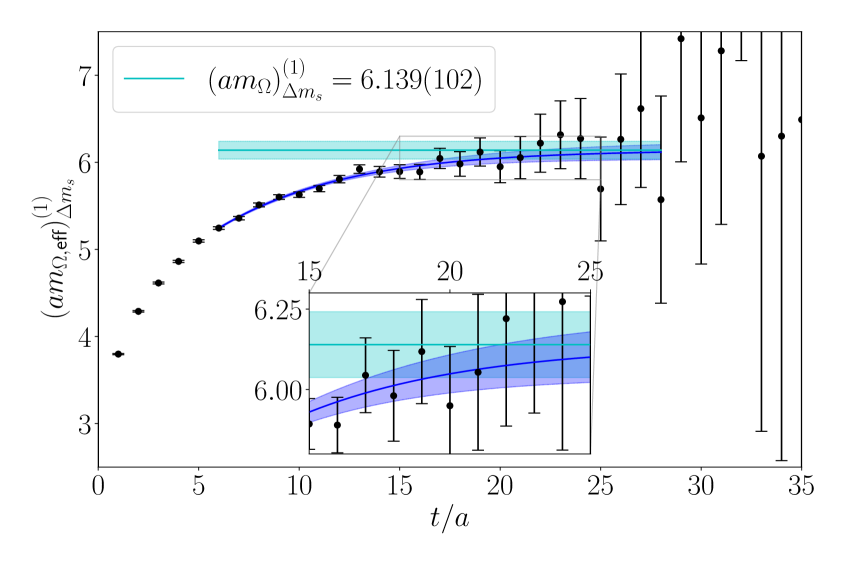
Figure 1: Effective mass plots and fits of the $\Omega$ baryon for the isospin-symmetric case (top), the QED corrections (lower left), and the $\Delta m_{s}$ corrections (lower right) on D450. The blue bands show the results of two-state fits according to eqs. 5 and 6. Their asymptotic values which correspond to the ground state mass or its corrections are shown in cyan. The fit interval is indicated by the horizontal extent of the blue and cyan lines. The effective masses are computed via eq. 2.

An example for the fits of all contributions of the $\Omega$-baryon on D450 is shown in fig. 1. The fit intervals were chosen according to the criteria discussed above. The smaller insets illustrate the aforementioned problem of a late onset of a plateau, since the deviation of the fit curve from the asymptotic value is comparable to the error of the effective mass around $t/a=20$ where the statistical fluctuations of the first-order correlation functions become uncontrollably large. As the $\Omega$ is among the least noisy baryon channels, this problem is often more severe for other baryons.

By looking at the different members of the baryon octet and decuplet, we found that the most promising candidates to use for setting the scale in terms of precision are the $\Omega$ and the $\Xi$. The values for the isospin-symmetric masses and their corrections we find from our analysis of N451 and D450 data in lattice units are listed in table 1.

Table 1: Preliminary results for the most promising candidates for scale setting on the CLS ensembles N451 and D450. The different columns represent different contributions in the isospin-breaking expansion. $\delta(am_{0})$ denotes the shift of the ground-state mass due to the isospin-breaking corrections shown in the other columns. To obtain this value we use results for the isospin-breaking parameters from another study using the hadronic renormalization scheme described in [22]. All uncertainties are purely statistical.

ensemble	baryon	$am_{0}^{(0)}$	$(am_{0})_{e^{2}}^{(1)}$	$(am_{0})_{\Delta m_{u/d}}^{(1)}$	$(am_{0})_{\Delta m_{s}}^{(1)}$	$\delta(am_{0})$
N451	$\Omega^{-}$	$0.5970(23)\text{\,}$	$0.1430(25)\text{\,}$	-	$5.90(10)\text{\,}$	$0.000\,20(2)\text{\,}$
	$\Xi^{-}$	$0.4777(14)\text{\,}$	$0.2031(18)\text{\,}$	$3.303(61)\text{\,}$	$5.160(24)\text{\,}$	$0.001\,26(3)\text{\,}$
	$\Xi^{+}$	$0.4777(14)\text{\,}$	$0.4326(60)\text{\,}$	$3.303(61)\text{\,}$	$5.160(24)\text{\,}$	$-0.000\,85(3)\text{\,}$
D450	$\Omega^{-}$	$0.6116(25)\text{\,}$	$0.1504(26)\text{\,}$	-	$6.14(10)\text{\,}$	$0.000\,24(7)\text{\,}$
	$\Xi^{-}$	$0.4876(11)\text{\,}$	$0.2003(29)\text{\,}$	$3.198(78)\text{\,}$	$5.077(32)\text{\,}$	$0.001\,32(17)\text{\,}$
	$\Xi^{+}$	$0.4876(11)\text{\,}$	$0.423(11)\text{\,}$	$3.198(78)\text{\,}$	$5.077(32)\text{\,}$	$-0.000\,76(60)\text{\,}$

Our estimates for the mass shifts are based on results from a previous calculation [23, 22], where the isospin breaking parameters $e^{2}=4\pi\alpha_{\text{em}}$, $\Delta m_{d}$, $\Delta m_{u}$, and $\Delta m_{s}$ were determined by identifying the following quantities in QCD+QED with their experimentally measured values:

$$\begin{aligned} \quantity(m_{\pi^{0}}^{2})^{\text{QCD+QED}}=&\quantity(m_{\pi^{0}}^{2})^{\text{experiment}},\\ \quantity(m_{K^{+}}^{2}+m_{K^{0}}^{2}-m_{\pi^{+}}^{2})^{\text{QCD+QED}}=&\quantity(m_{K^{+}}^{2}+m_{K^{0}}^{2}-m_{\pi^{+}}^{2})^{\text{experiment}},\\ \quantity(m_{K^{+}}^{2}-m_{K^{0}}^{2}-m_{\pi^{+}}^{2}+m_{\pi^{0}}^{2})^{\text{QCD+QED}}=&\quantity(m_{K^{+}}^{2}-m_{K^{0}}^{2}-m_{\pi^{+}}^{2}+m_{\pi^{0}}^{2})^{\text{experiment}},\\ \quantity(\alpha_{\text{em}})^{\text{QCD+QED}}=&\quantity(\alpha_{\text{em}})^{\text{experiment}}.\end{aligned}$$ (7)

These conditions must be evaluated for each ensemble individually, and in order to perform this matching, a lattice scale has to be used in order to calculate the masses in physical units from the lattice results. As we have no results for the lattice scale including isospin-breaking corrections thus far, the masses computed on the lattice were scaled with a value from purely isospin-symmetric results. The results from this matching which are used to compute $\delta(am_{0})$ in table 1 are

Ensemble	$a\Delta m_{d}$	$a\Delta m_{u}$	$a\Delta m_{s}$
N451	$-0.001\,837\,4(71)\text{\,}$	$-0.008\,847\,4(75)\text{\,}$	$-0.002\,189\,0(18)\text{\,}$
D450	$-0.001\,816\,0(73)\text{\,}$	$-0.008\,845\,7(82)\text{\,}$	$-0.002\,212\,3(61)\text{\,}$

.

For the baryons listed in table 1 we find that on the given ensembles we reach a precision of better than $0.5\text{\,}\mathrm{\char 37\relax}$, with the size of isospin-breaking corrections being of the same order as the zeroth-order uncertainty or even smaller. However, these uncertainty estimates are purely statistical and systematics still have to be investigated for a realistic estimate of the uncertainties. Since we do not take corrections in the sea-quark sector into account, for example, the listed isospin-breaking contributions are incomplete which has to be considered as a systematic uncertainty. Furthermore, isospin-breaking corrections of the lattice scale have been neglected in the matching in eq. 7, and finite-volume effects were not considered in any of our results presented here.

For the $\Omega$ baryon we find only very small mass shifts arising from isospin-breaking effects. This is not surprising and is one of the reasons this baryon is generally a popular candidate for scale-setting [24, 25, 26].

5 Conclusion and Outlook

We have presented our method for the determination of baryon octet and decuplet masses and their corrections due to isospin-breaking effects from correlation functions computed as described in [14]. We found that small statistical uncertainties on these quantities can be achieved for the $\Omega$ and $\Xi^{\pm}$ baryons which we therefore consider as prime candidates for setting the scale of CLS $N_{f}=2+1$ ensembles. As we have only processed two ensembles so far, we are currently extending our analysis to additional ensembles, in order to thoroughly investigate the suitability of our baryonic mass estimates for scale setting.

References

- [1] H.B. Meyer and H. Wittig, Lattice QCD and the anomalous magnetic moment of the muon, Prog. Part. Nucl. Phys. 104 (2019) 46 [1807.09370].
- [2] RM123 collaboration, Isospin-breaking effects due to the up-down mass difference in Lattice QCD, JHEP 04 (2012) 124 [1110.6294].
- [3] RM123 collaboration, Leading isospin-breaking effects on the lattice, Phys. Rev. D 87 (2013) 114505 [1303.4896].
- [4] M. Bruno, T. Korzec and S. Schaefer, Setting the scale for the CLS flavor ensembles, Phys. Rev. D 95 (2017) 074504 [1608.08900].
- [5] B. Strassberger et al., Scale setting for CLS 2+1 simulations, PoS LATTICE2021 (2022) 135 [2112.06696].
- [6] N. Carrasco, V. Lubicz, G. Martinelli, C.T. Sachrajda, N. Tantalo, C. Tarantino et al., QED Corrections to Hadronic Processes in Lattice QCD, Phys. Rev. D 91 (2015) 074506 [1502.00257].
- [7] M. Bruno et al., Simulation of QCD with N 2 1 flavors of non-perturbatively improved Wilson fermions, JHEP 02 (2015) 043 [1411.3982].
- [8] M. Lüscher, S. Sint, R. Sommer and P. Weisz, Chiral symmetry and O(a) improvement in lattice QCD, Nucl. Phys. B 478 (1996) 365 [hep-lat/9605038].
- [9] J. Bulava and S. Schaefer, Improvement of = 3 lattice QCD with Wilson fermions and tree-level improved gauge action, Nucl. Phys. B 874 (2013) 188 [1304.7093].
- [10] S. Güsken, A Study of smearing techniques for hadron correlation functions, Nucl. Phys. B Proc. Suppl. 17 (1990) 361.
- [11] APE collaboration, Glueball Masses and String Tension in Lattice QCD, Phys. Lett. B 192 (1987) 163.
- [12] UKQCD collaboration, Gauge invariant smearing and matrix correlators using Wilson fermions at Beta = 6.2, Phys. Rev. D 47 (1993) 5128 [hep-lat/9303009].
- [13] Lattice Hadron Physics (LHPC) collaboration, Clebsch-Gordan construction of lattice interpolating fields for excited baryons, Phys. Rev. D 72 (2005) 074501 [hep-lat/0508018].
- [14] A.M. Segner, A.D. Hanlon, R.J. Hudspith, A. Risch and H. Wittig, Isospin-breaking Effects in Octet and Decuplet Baryon Masses, PoS LATTICE2021 (2022) 095 [2112.08262].
- [15] T. Blum, T. Izubuchi and E. Shintani, Error reduction technique using covariant approximation and application to nucleon form factor, PoS LATTICE2012 (2012) 262 [1212.5542].
- [16] T. Blum, T. Izubuchi and E. Shintani, New class of variance-reduction techniques using lattice symmetries, Phys. Rev. D 88 (2013) 094503 [1208.4349].
- [17] E. Shintani, R. Arthur, T. Blum, T. Izubuchi, C. Jung and C. Lehner, Covariant approximation averaging, Phys. Rev. D 91 (2015) 114511 [1402.0244].
- [18] G.P. Lepage, The Analysis of Algorithms for Lattice Field Theory, in Theoretical Advanced Study Institute in Elementary Particle Physics, 6, 1989.
- [19] M.L. Wagman and M.J. Savage, Statistics of baryon correlation functions in lattice QCD, Phys. Rev. D 96 (2017) 114508 [1611.07643].
- [20] L. Del Debbio, L. Giusti, M. Luscher, R. Petronzio and N. Tantalo, QCD with light Wilson quarks on fine lattices (I): First experiences and physics results, JHEP 02 (2007) 056 [hep-lat/0610059].
- [21] M. Lüscher, Properties and uses of the Wilson flow in lattice QCD, JHEP 08 (2010) 071 [1006.4518].
- [22] A. Risch and H. Wittig, Leading isospin breaking effects in the HVP contribution to and to the running of , PoS LATTICE2021 (2022) 106 [2112.00878].
- [23] A. Risch and H. Wittig, Towards leading isospin-breaking effects in mesonic masses with open boundaries, PoS LATTICE2018 (2018) 059 [1811.00895].
- [24] RBC-UKQCD collaboration, Physical Results from 2+1 Flavor Domain Wall QCD and SU(2) Chiral Perturbation Theory, Phys. Rev. D 78 (2008) 114509 [0804.0473].
- [25] S. Borsányi et al., Leading hadronic contribution to the muon magnetic moment from lattice QCD, Nature 593 (2021) 51 [2002.12347].
- [26] N. Miller et al., Scale setting the Möbius domain wall fermion on gradient-flowed HISQ action using the omega baryon mass and the gradient-flow scales and , Phys. Rev. D 103 (2021) 054511 [2011.12166].