Temperature Dependence of Gluon and Ghost Propagators in a Dyson-Schwinger Equations context

Abstract

We investigate the finite-temperature structure of ghost and gluon propagators within an approach based on the rainbow truncated Dyson-Schwinger equations in Landau gauge. The method, early used for modeling the quark, ghost and gluon propagators in vacuum, is extended to finite temperatures. In Euclidean space, within the Matsubara imaginary-time formalism it is necessary to distinguish between the transversal and longitudinal, with respect to the heat bath, gluon dressing functions, for which the Dyson-Schwinger equation splits into a corresponding system of coupled equations. This system is considered within the rainbow approximation generalized to finite temperatures and solved numerically. The solutions for the ghost and gluon propagators are obtained as functions of temperature $\displaystyle T$, Matsubara frequency $\displaystyle\Omega_{n}$ and three-momentum squared $\displaystyle{\bf k}^{2}$. The effective parameters of the approach are taken from our previous fit of the corresponding Dyson-Schwinger solution to the lattice QCD data at zero temperature. In solving the coupled system of the Dyson-Schwinger equations at finite temperatures, the model parameters are treated as constants, independent on temperature. It is found that, for zero Matsubara frequency, the dependence of the ghost and gluon dressing functions on $\displaystyle{\bf k}^{2}$ are not sensitive to the temperature $\displaystyle T$, while at $\displaystyle{\bf k}^{2}=0$ their dependence on $\displaystyle T$ is quite strong. Dependence on the Matsubara frequency $\displaystyle\Omega_{n}$ is investigated as well. The performed numerical analysis of the solution of the Dyson-Schwinger equations shows that at certain value of the temperature $\displaystyle T_{0}\sim 150$ MeV the iteration procedure does not longer converge. In the vicinity of $\displaystyle T_{0}$ the longitudinal gluon propagator increases quite fastly, whereas the transversal propagator does not exhibit any irregularity. This in a qualitative agreement with results obtained within the QCD lattice calculations in this temperature interval.

I Introduction

The study of the behaviour of hadrons in hot and dense nuclear matter is among the most interesting and challenging problems intensively investigated by theorists and experimentalists. It is tightly connected to studies of the quark-gluon plasma (QGP) which is the deconfined phase of the strongly interacting QCD. It is commonly adopted that this phase existed in the early universe and can also be briefly produced in laboratory by heavy-ion collisions. This stimulates intensive studies of high energy processes with heavy ions. A bulk of the running and projected experiments in various research centers, e.g. at Belle (Japan), BESIII (Beijing, China), LHC (CERN), GlueX (JLAB, USA), NICA (Dubna, Russia), HIAF (China), FAIR (GSI, Germany) etc., include in their research programmes comprehensive investigations of properties of hadrons at high temperatures and the possible transition to quark-gluon plasma. Appropriate approaches in theoretical study of properties of quarks and gluons at zero and finite temperature are the lattice QCD simulations GhostLatticeMishaPRD ; BornyakovLattice ; Aouane:2011fv ; Ilgenfritz:2017kkp ; LatticeQuenchedvsUnquenched ; QuenchedUnquenchedGluon ; Albanese ; Chen ; Morningstar , complemented by functional renormalization group (FRG) methods (see e.g. Refs. Dupuis:2020fhh ; PawlowskyFRG ), approaches based on QCD Sum Rules Shifman:1978bx ; Shuryak:1982dp and the functional approaches via Dyson-Schwinger equations FisherTempQCD (for a review of different methods in studying gauge bosons at zero and finite temperatures, see Refs. MaasPhysReport ; Das ). Despite a fairly rigorous theoretical foundation, these approaches are rather complex and cumbersome in further applications in describing the temperature dependence of physical bound states, such as mesons and glueballs, for example. It is tempting therefore, to elaborate transparent models which, on the one hand, are simple and physically understandable, on the other hand, covering the main characteristics of the studied phenomena. In this lpaper, we employ a generalization of the well known rainbow approximation to the truncated Dyson-Schwinger equations (tDSE) alkof ; rober ; MT ; Dorkin:2014lxa to finite temperatures in Euclidean space within the imaginary-time formalism S-XQINprd84 ; Dorkin:2014lxa ; BlankKrass ; Viebakh ; dor .

The paper is organized as follows. In Sec. II we formulate the truncated system of Dyson-Schwinger equations for the ghost and gluon propagators at finite temperature within the Matsubara imaginary time formalism. The general expressions for the system of tDSE’s for ghost, transversal and longitudinal gluon propagators are presented. In Sec. III the rainbow approximation to the interaction kernels of the integral equations is defined. Further, in subsections  III.1 and III.2 this approximation is applied to perform explicitly the angular integrations in the ghost and gluon tDSE and to reduce the four-dimensional integral equations to summations over the Matsubara frequencies and one-dimensional integrations over the corresponding loop momenta. Results of numerical solutions of tDSE are presented in Sec. IV. The solution for the ghost dressing function and transversal and longitudinal gluon propagators are discussed in subsections IV.1 and IV.2, where the temperature and momentum dependence as well as the dependence on the Matsubara frequency, are analysed in some details. We summarize our conclusions in Sec. V.

II Coupled Dyson-Schwinger equations for gluons and ghosts

A nonperturbative continuum approach to QCD is provided by the Dyson-Schwinger equations. The system of Dyson-Schwinger coupled equations for the quark, ghost and gluon propagators and the vertex functions as well, being the equations of motion for the corresponding Green’s functions, can be considered as an alternative integral formulation of QCD. Evidently, attempts to solve exactly the system of these equations, which relate nonperturbatively $\displaystyle n$-point and $\displaystyle n+1$-point functions, thus constituting an infinite tower of coupled equations, fail to find adequate numerical solutions. Consequently, for practical purposes some approximations are necessary. Usually one employs truncations of the whole system by restricting oneself to only few first Feynman diagrams. Typically, the truncations contain only one-loop diagrams with dressed propagators and vertices, as depicted in Fig. 1 (cf., e.g. Ref. smekalAnnals267 ). The resulting system is referred to as the truncated Dyson-Schwinger equation (tDSE).

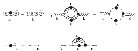
Figure 1: Diagrammatic representation of the employed Dyson-Schwinger equations for ghost (top line) and gluon (bottom line) propagators. The internal wiggly and dashed lines denote the full, marked by filled blobs, gluon and ghost propagators, respectively. The irreducible one-particle vertices are also denoted by filled blobs. In the gluon Dyson-Schwinger equation, terms with four-gluon vertices and quark loops have been dismissed.

Note that this subset is already strongly reduced relative to the full set of equivalent QCD diagrams, discussed in e.g. FisherTempQCD in a wider context and even relative to the subset of one-loop diagrams. It does contain neither loops with four-gluon vertices nor quark loops. The four-gluon vertices are the momentum independent tadpole-like terms and terms with explicit two-loop contributions. While the former leads an irrelevant constant which vanishes perturbatively in Landau gauge, the latter are subleading in the infrared, cf. Ref. smekalAnnals267 . As for ignoring quark loops, it can be justified by the observation LatticeQuenchedvsUnquenched ; QuenchedUnquenchedGluon ; fisher that in the tDSE the unquenching effects are rather small for the dynamical quark masses. For the gluon dressing function, such effects are seen only in the neighbourhood of its maximum at $\displaystyle k\sim 0.85-1.0\,{\rm GeV/c}$, where the screening effect from the creation of quark-antiquark pairs from the vacuum slightly decreases the value of the gluon dressing. In our approach, this effect is implicitly taken into account by adjusting the phenomenological parameters at zero temperature to full, unquenched lattice calculations, see e.g. Refs.  GhostLatticeMishaPRD ; BornyakovLattice for SU(2) lattice QCD data.

The system of coupled tDS equations for the gluon and ghost propagators is obtained by direct calculation of the corresponding one-loop Feynman diagrams in Fig. 1. In Landau gauge, the resulting system can be written as

$$\displaystyle D_{\mu\nu}^{-1}(k_{4}^{2},{\bf k}^{2})=Z_{3}D_{0\,\mu\nu}^{-1}(k^{2})+\Sigma^{gluon}_{\mu\nu}(k_{4}^{2},{\bf k}^{2})+\Sigma^{ghost}_{\mu\nu}(k_{4}^{2},{\bf k}^{2}),$$ (1)

$$\displaystyle D_{G}^{-1}(k_{4}^{2},{\bf k}^{2})=\tilde{Z}_{3}D_{0G}^{-1}(k^{2})+S^{ghost}(k_{4}^{2},{\bf k}^{2}).$$ (2)

where $\displaystyle Z_{3}$ and $\displaystyle\tilde{Z}_{3}$ are the gluon and ghost renormalization constants, respectively, $\displaystyle D_{0\,\mu\nu}(k^{2})$ and $\displaystyle D_{0G}(k^{2})$ denote the corresponding free propagators, $\displaystyle k^{2}=k_{4}^{2}+{\bf k}^{2}$ and the self-energy terms $\displaystyle\Sigma^{gluon}_{\mu\nu}(k_{4},{\bf k})$, $\displaystyle\Sigma^{ghost}_{\mu\nu}(k_{4},{\bf k})$ and $\displaystyle S^{ghost}(k_{4},{\bf k})$ correspond to the three loop diagrams depicted in Fig. 1. In Euclidean space, at zero temperatures the gluon and ghost propagators are

$$D_{\mu\nu}^{ab}(k^{2})=\delta^{ab}D_{\mu\nu}(k^{2})=\delta^{ab}\left(\delta_{\mu\nu}-\frac{k_{\mu}k_{\nu}}{k^{2}}\right)\frac{Z(k^{2})}{k^{2}};\quad D_{G}^{ab}(k^{2})=\delta^{ab}D_{G}(k^{2})=-\delta^{ab}\frac{G(k^{2})}{k^{2}},$$ (3)

where $\displaystyle a,b$ are the color indices and $\displaystyle Z(k^{2})$ and $\displaystyle G(k^{2})$ are the gluon and ghost dressing functions, respectively.

At finite temperatures, within the imaginary time formalism all the relevant four-momenta in Euclidean space possess discrete spectra of the corresponding fourth component, $\displaystyle k_{4}=\Omega_{n}$ ($\displaystyle n\subset\mathbb{Z}$), where $\displaystyle\Omega_{n}=2\pi nT$ for bosons (gluons) and $\displaystyle\Omega_{n}=\pi(2n+1)T$ for fermions (quarks). As for the Fadeev-Popov ghosts, in spite of the Grassmann nature of their fields needed in the gauge fixing procedure, formally ghosts are related to (nonexisting) spin-zero particles and to scalar propagators. Consequently, the ghost fields satisfy periodic conditions like any bosonic field, cf. Refs. Das ; Gruter ; Bernard ; Gross , so that the Mtzubara frequencies for ghosts are even .

In Landau gauge, the Euclidean gluon propagator $\displaystyle{\cal D}_{\mu\nu}^{ab}(k_{4},{\bf k})$ and ghost propagator $\displaystyle{\cal D}_{G}^{ab}(k_{4},{\bf k})$ are expressed via the dressing functions $\displaystyle Z(k_{4},{\bf k})$ and $\displaystyle G(k_{4},{\bf k})$ as

$$\displaystyle{\cal D}_{\mu\nu}^{ab}(k)=\delta^{ab}{D}_{\mu\nu}(k_{4},{\bf k})=\delta^{ab}\left\{\frac{Z_{T}(k_{4},{\bf k})}{k^{2}}{\cal P}^{T}_{\mu\nu}({\bf k})+\frac{Z_{L}(k_{4},{\bf k})}{k^{2}}{\cal P}^{L}_{\mu\nu}(k_{4},{\bf k})\right\},$$ (4)

$$\displaystyle{\cal D}_{G}^{ab}(k_{4},{\bf k})=-\delta^{ab}D_{G}(k_{4},{\bf k})=-\delta^{ab}\frac{G(k_{4},{\bf k})}{k^{2}},$$ (5)

where $\displaystyle{\cal P}^{L}_{\mu\nu}(k_{4},{\bf k})$, and $\displaystyle{\cal P}^{T}_{\mu\nu}({\bf k})$ are the longitudinal and transversal, in 3D space, projectors,

$$\displaystyle{\cal P}^{T}_{\mu\nu}({\bf k})=\left\{\begin{array}[]{llll}0,&&\mu\ {\rm and/or}\ \nu=4,\\ \delta_{\alpha\beta}-\dfrac{k_{\alpha}k_{\beta}}{{\bf k}^{2}};&&\mu,\nu=\alpha,\beta=1,2,3,\end{array}\right.$$ (8)

$$\displaystyle{\cal P}^{L}_{\mu\nu}(k)={\cal P}_{\mu\nu}(k)-{\cal P}^{T}_{\mu\nu}({\bf k});\quad{\rm where}\quad{\cal P}_{\mu\nu}(k)=\delta_{\mu\nu}-\dfrac{k_{\mu}k_{\nu}}{k^{2}}.$$ (9)

Note that these projection operators are four-dimensionally transverse and have the properties

$${\cal P}^{T}{\cal P}^{T}={\cal P}^{T},\,{\cal P}^{L}{\cal P}^{L}={\cal P}^{L},\,{\cal P}^{T}{\cal P}^{L}={\cal P}^{L}{\cal P}^{T}=0,\quad{\cal P}^{T}_{\mu\nu}{\cal P}^{T}_{\mu\nu}=2,\,{\cal P}^{L}_{\mu\nu}{\cal P}^{L}_{\mu\nu}=1.$$ (10)

Relations (10) are widely used in deriving the Dyson-Schwinger equations for transverse and longitudinal dressing functions $\displaystyle Z_{(T,L)}$ from eqs. (1)-(4). It should be noted that, in an arbitrary gauge the gluon propagator reads as

$$\displaystyle{\cal D}_{\mu\nu}(k)=\frac{Z_{T}(k_{4},{\bf k})}{k^{2}}{\cal P}^{T}_{\mu\nu}({\bf k})+\frac{Z_{L}(k_{4},{\bf k})}{k^{2}}{\cal P}^{L}_{\mu\nu}(k_{4},{\bf k})+\frac{\eta}{k^{2}}\frac{k_{\mu}k\nu}{k^{2}},$$ (11)

where $\displaystyle\eta$ is the gauge parameter. The inverse of (11 ) is

$$\displaystyle{\cal D}_{\mu\nu}^{-1}(k)=\frac{k^{2}}{Z_{T}(k_{4},{\bf k})}{\cal P}^{T}_{\mu\nu}({\bf k})+\frac{k^{2}}{Z_{L}(k_{4},{\bf k})}{\cal P}^{L}_{\mu\nu}(k_{4},{\bf k})+\frac{k^{2}}{\eta}\frac{k_{\mu}k_{\nu}}{k^{2}}.$$ (12)

It can be seen that in Landau gauge ($\displaystyle\eta=0$) the inverse gluon propagator becomes ill-defined. However, since the longitudinal part of the propagator $\displaystyle\eta\frac{k_{\mu}k\nu}{k^{2}}$ is not affected by the renormalization procedure, in Eq. (1) the terms with $\displaystyle\eta^{-1}$ in the left hand side and right hand side cancel each other and the resulting equation remains well defined. Generally, performing calculations with propagators in the Landau gauge one shall use the propagator in the form of Eq. (11) and take the limit $\displaystyle\eta\to 0$ at the end of calculations. In our case the tDSE, Eq. (1), does not depend on $\displaystyle\eta$ and, consequently, we can neglect such terms from the very beginning and write Eq. (1) as

$$\displaystyle\frac{k^{2}}{Z_{T}(k_{4},{\bf k})}{\cal P}^{T}_{\mu\nu}({\bf k})+\frac{k^{2}}{Z_{L}(k_{4},{\bf k})}{\cal P}^{L}_{\mu\nu}(k_{4},{\bf k})=Z_{3}k^{2}{\cal P}_{\mu\nu}(k)+\Sigma^{gluon}_{\mu\nu}(k_{4}^{2},{\bf k}^{2})+\Sigma^{ghost}_{\mu\nu}(k_{4}^{2},{\bf k}^{2}).$$ (13)

Then, after contracting the color indices in the corresponding loops in Fig. 1, the self-energy parts explicitly read as

$$\displaystyle\Sigma^{gluon}_{\mu\nu}(\Omega_{n},{\bf k}) \displaystyle=\frac{1}{2}\frac{3T}{2\pi^{2}}\sum_{m}\int d^{3}q\Gamma_{\mu\alpha\rho}^{(0)}(k,-q,p)\frac{Z_{T}(\Omega_{m},{\bf q}){\cal P}^{T}_{\alpha\beta}({\bf q})+Z_{L}(\Omega_{m},{\bf q}){\cal P}^{L}_{\alpha\beta}}{q^{2}}\bigg{[}\frac{g^{2}}{4\pi}\times$$ (14)

$$\displaystyle\Gamma_{\beta\nu\sigma}(q,-p,-k)\left(D_{T}(\Omega_{mn},{\bf p}){\cal P}^{T}_{\sigma\rho}({\bf p})+D_{L}(\Omega_{mn},{\bf p}){\cal P}^{L}_{\sigma\rho}(p)\right)\bigg{]},$$

$$\displaystyle\Sigma^{ghost}_{\mu\nu}(\Omega_{n},{\bf k}) \displaystyle=-\frac{3T}{2\pi^{2}}\sum_{m}\int d^{3}q\frac{G(\Omega_{m},{\bf q})}{q^{2}}\left[\Gamma^{(0)}_{\mu}(q)\frac{g^{2}}{4\pi}D_{G}(\Omega_{mn},{\bf p})\Gamma_{\nu}(p)\right],$$ (15)

$$\displaystyle S^{ghost}(\Omega_{n},{\bf k}) \displaystyle=\frac{3T}{2\pi^{2}}\sum_{m}\int d^{3}q\left[\frac{g^{2}}{4\pi}\Gamma_{\mu}^{(0)}(q)D_{\mu\nu}(p^{2})\Gamma_{\nu}(k,q,p)\right]\frac{G(\Omega_{m},{\bf q})}{q^{2}},$$ (16)

where $\displaystyle p=q-k$, $\displaystyle p_{4}\equiv\Omega_{mn}=\Omega_{m}-\Omega_{n}$, $\displaystyle{\bf p}={\bf q}-{\bf k}$ and the terms enclosed in the square brackets define the interaction kernel of the corresponding integral equation. In the above expressions we have taken into account that due to periodicity of the gluon and ghost fields, the integration over the fourth component $\displaystyle dq_{4}$ is replaced by the summation over the discrete Matsubara frequencies according to

$$\int\limits_{-\infty}^{\infty}\frac{dq_{4}}{2\pi}\int\frac{d^{3}q}{(2\pi)^{3}}f(q_{4},{\bf q})\rightarrow T\sum\limits_{n=-\infty}^{\infty}\int\frac{d^{3}q}{(2\pi)^{3}}f(\Omega_{n},{\bf q}).$$ (17)

The tDSE for the scalar dressing functions $\displaystyle Z_{T,L}$ are obtained from the tDSE (1) by inserting Eqs. (14)-(15) in to Eq. (1), multiplying the left and right hand sides consecutively by $\displaystyle{\cal P}^{T}(\Omega_{n},{\bf k})$ and $\displaystyle{\cal P}^{L}(\Omega_{n},{\bf k})$ and contracting all the Lorentz indices.

The gluon renormalization constants $\displaystyle Z_{3(T,L)}$ for transverse and longitudinal propagators, in principle, can be different and must be determined separately. In the present paper, for the sake of simplicity, we adopt the renormalization constant $\displaystyle Z_{3}$ to be the same for both, transverse and longitudinal parts. Moreover, the concrete numerical values for $\displaystyle Z_{3}$ and $\displaystyle\tilde{Z}_{3}$ are taken from the previous fit ourGlueball of the tDSE solution in vacuum to the lattice QCD data, viz. $\displaystyle Z_{3}=\tilde{Z}_{3}\approx 1.065$.

III Rainbow approximation

Attempts to solve the system of coupled equations by employing directly the QCD Feynman rules encounter difficulties related to regularizations of divergent loop integrals and to symmetry constraints on gluon-ghost and three-gluon vertices, such as Slavnov-Taylor identities. Clearly, further approximations are required. In vacuum, the simplest approximation consists in replacements of the fully dressed three-gluon and ghost-gluon vertices by their bare values, known as the Mandelstam approximation CPCMandelstam ; MANDELSTAM_Approx ; PennigtonMandels and as the y-max approximation YmaxApprox . Within these approaches, in order to facilitate the angular integrations in analytical and numerical analysis of Eqs. (1) - (2), additional simplifications for the momentum dependence in $\displaystyle Z(k^{2})$ and $\displaystyle G(k^{2})$ have been adopted. Also, some ansatzs for infrared and ultraviolet asymptotic solution $\displaystyle Z(k^{2})$ and $\displaystyle G(k^{2})$ have been adopted. A more rigorous analysis of the tDSE has been presented in a series of publications in Refs. IRGluonProp_AlkoferSmekal ; smekalAnnals267 (see also the review Ref. AlkoferphysRep and references therein quoted). All the above mentioned approaches result in rather cumbersome expressions for the system of tDSE’s which, consequently, cause difficulties in finding the numerical solutions. Moreover, these circumstances are more significant in attempts to solve the tDSE at finite temperatures. In order to avoid the mentioned difficulties and to simplify the angular integrations, in the present paper we employ a rainbow-like approximation, similar to the rainbow model alkof ; rober ; BlankKrass ; Viebakh ; dor , for the interaction kernels enclosed in square brackets in Eqs. (14) - (16). This approximation consists in replacing the dressed vertices together with the dressed exchanging propagators by their bare quantities augmented by some effective form factors:

$$\displaystyle\left[\frac{g^{2}}{4\pi}\Gamma_{\mu\alpha\rho}^{(0)}(k,-q,p)D_{\rho\sigma}(p^{2})\Gamma_{\beta\nu\sigma}(q,-p,-k)\right]=$$

$$\displaystyle\Gamma_{\mu\alpha\rho}^{(0)}(k,-q,p)\bigg{[}{\cal P}^{T}_{\rho\sigma}({\bf p})F^{T}_{1}(p^{2})+{\cal P}^{L}_{\rho\sigma}(p)F^{L}_{1}(p^{2})\bigg{]}\Gamma_{\beta\nu\sigma}^{(0)}(q,-k,-p),$$ (18)

$$\displaystyle\left[\frac{g^{2}}{4\pi}\Gamma_{\mu}^{(0)}(q)D_{G}(p^{2})\Gamma_{\nu}(k)\right]=\Gamma_{\mu}^{(0)}(q)F_{2}(p^{2})\Gamma_{\nu}^{(0)}(p^{2}),$$ (19)

$$\displaystyle\bigg{[}\frac{g^{2}}{4\pi}\Gamma^{(0)}_{\mu}(q)D_{\mu\nu}(p^{2})\Gamma_{\nu}(k,q,p)\bigg{]}=\Gamma_{\mu}^{(0)}(q)\left[{\cal P}^{T}_{\mu\nu}({\bf p})F^{T}_{3}(p^{2})+{\cal P}^{L}_{\mu\nu}(p)F^{L}_{3}(p^{2})\right]\Gamma_{\nu}^{(0)}(k),$$ (20)

where the superscript (0) of the vertex functions $\displaystyle\Gamma$ means the free 3-gluon and free ghost-gluon-ghost vertices (see Ref. ourGlueball for more details). As in Ref. ourGlueball , we use for the form-factors $\displaystyle F_{1-3}(p^{2})$ a Gaussian form with two terms for each formafactor $\displaystyle F_{1-3}(p^{2})$. This is quite sufficient to obtain a reliable solution of the system of tDS equations at $\displaystyle T=0$ when the O(4) symmetry holds exactly and consequently, the longitudinal and transversal part of the gluon propagator coincide. Explicitly, in Euclidean space the effective form factors are chosen as

$$\displaystyle F^{T,L}_{1}(p^{2})=D^{T,L}_{11}\frac{p^{2}}{(\omega_{11}^{T,L})^{6}}e^{-p^{2}/(\omega_{11}^{T,L})^{2}}+D^{T,L}_{12}\frac{p^{2}}{(\omega_{12}^{T,L})^{6}}e^{-p^{2}/(\omega_{12}^{T,L})^{2}},$$ (21)

$$\displaystyle F_{2}(p^{2})=\frac{D_{21}}{\omega_{21}^{4}}e^{-p^{2}/\omega_{21}^{2}}+\frac{D_{22}}{\omega_{22}^{4}}e^{-p^{2}/\omega_{22}^{2}},$$ (22)

$$\displaystyle F^{T,L}_{3}(p^{2})=D^{T,L}_{31}\frac{p^{2}}{(\omega_{31}^{T,L})^{6}}e^{-p^{2}/(\omega_{31}^{T,L})^{2}}+D^{T,L}_{32}\frac{p^{2}}{(\omega_{32}^{T,L})^{6}}e^{-p^{2}/(\omega_{32}^{T,L})^{2}},$$ (23)

with phenomenological parameters $\displaystyle D_{i}$ and $\displaystyle\omega_{i}$ fitted to provide a reasonable good description of the lattice SU(2) data at zero temperatures (cf. Ref. ourGlueball ).

III.1 The tDSE for the ghost propagator, Fig. 1, bottom line

With the effective interaction eqs. (18)-(23), the angular integration can be carried out analytically ourGlueball resulting in a system of linear algebraic equations with respect to the Matsubara frequency and one-dimensional integral equations with respect to three-momentum $\displaystyle|{\bf k}|$ in Euclidean space. Explicitly, by using the reltaions $\displaystyle\Gamma_{\mu}^{(0)}(q)=-iq_{\mu}$ and $\displaystyle\Gamma_{\nu}^{(0)}(k)=-ik_{\nu}$ and $\displaystyle q_{\mu}\,{\cal P}^{(T,L)}_{\mu\nu}(p)k_{\nu}=q_{\mu}{\cal P}^{(T,L)}_{\mu\nu}(p)\,q_{\nu}$ and Eqs. (2), (9) and (15), the tDSE for ghosts reads as

$$\displaystyle\frac{1}{G(\Omega_{n},{\bf k})}=\tilde{Z}_{3}-\frac{3}{2\pi^{2}}T\sum_{m}\int d^{3}q\frac{G(\Omega_{m},{\bf q})}{k^{2}q^{2}}\left[\Delta F_{3}(p^{2})q_{\mu}{\cal P}^{T}_{\mu\nu}({\bf p})q_{\nu}+F_{3}^{L}(p^{2})q_{\mu}P_{\mu\nu}(p)q_{\nu}\right],$$ (24)

where $\displaystyle q=p+k$, $\displaystyle\Delta F_{3}(p^{2})=F_{3}^{T}(p^{2})-F_{3}^{L}(p^{2})$ and

$$q_{\mu}{\cal P}^{T}_{\mu\nu}({\bf p})q_{\nu}=\frac{{\bf q}^{2}{\bf k}^{2}}{{\bf p^{2}}}\sin^{2}\theta_{\bf kq};\quad q_{\mu}P_{\mu\nu}(p)k_{\nu}=q_{\mu}P_{\mu\nu}(p)q_{\nu}=\frac{q^{2}k^{2}-(qk)^{2}}{p^{2}}.$$ (25)

In the limit $\displaystyle T\to 0$ the $\displaystyle O(4)$ symmetry is restored, i.e. $\displaystyle\Delta F_{3}(p^{2})=0$, $\displaystyle T\sum\limits_{m}\to\int\limits_{-\infty}^{\infty}\displaystyle\frac{dq_{4}}{2\pi}$ and

$$\displaystyle\!\!\!\!\!\!\frac{1}{G(k^{2})}=\tilde{Z}_{3}-\sum_{j=1}^{2}\frac{3}{\pi^{2}}\int q^{3}dq\frac{G(q^{2})D_{3j}^{L}}{(\omega_{3j}^{L})^{6}}\exp\left(-(k^{2}+q^{2}-2kq\cos\chi_{kq})/(\omega_{3j}^{L})^{2}\right)\sin^{4}\chi_{qk}d\chi_{qk},$$ (26)

where $\displaystyle\chi_{qk}$ is the hyper-angle between the 4-momenta $\displaystyle k$ and $\displaystyle q$.

By taking into account that

$$\int\exp\left[2kq\cos\chi_{kq})/(\omega_{3j}^{L})^{2}\right])\sin^{4}\chi_{qk}d\chi_{qk}=\frac{3\pi}{4}\frac{(\omega_{3j}^{L})^{4}}{k^{2}q^{2}}I_{2}\left(\frac{2kq}{(\omega_{3j}^{L})^{2}}\right),$$ (27)

where $\displaystyle I_{2}\left(\frac{2kq}{\omega_{3j}^{L})^{2}}\right)$ is the modified Bessel function, the ghost DSE in vacuum is recovered ourEPJP .

Coming back to finite temperatures, Eq. (24), the DSE for ghosts within rainbow approximation (23) reads as

$$\displaystyle\frac{1}{G(\Omega_{n},{\bf k})}=\tilde{Z}_{3}-\frac{3T}{2\pi^{2}}\sum_{m=-\infty}^{\infty}\sum_{j=1}^{2}\int d{\bf q}\frac{G(\Omega_{m},{\bf q})}{k^{2}q^{2}}\bigg{\{}{\rm e}^{-p^{2}/(\omega_{3j}^{L})^{2}}\frac{D^{L}_{3j}}{(\omega_{3j}^{L})^{6}}\big{[}k^{2}q^{2}-(kq)^{2}\big{]}+$$

$$\displaystyle{\bf k}^{2}{\bf q}^{2}\sin^{2}\theta_{{\bf q}{\bf k}}\bigg{[}1+\frac{\Omega_{mn}^{2}}{{\bf p}^{2}}\bigg{]}\bigg{[}\frac{D^{T}_{3j}}{(\omega_{3j}^{T})^{6}}{\rm e}^{-p^{2}/(\omega_{3j}^{T})^{2}}-\frac{D^{L}_{3j}}{(\omega_{3j}^{L})^{6}}{\rm e}^{-p^{2}/(\omega_{3j}^{L})^{2}}\bigg{]}\bigg{\}},$$ (28)

where $\displaystyle p^{2}=(\Omega_{n}-\Omega_{m})^{2}+{\bf q}^{2}+{\bf k}^{2}-2|{\bf k}||{\bf q}|\cos\theta_{{\bf q}{\bf k}}\,$, with $\displaystyle\theta_{{\bf q}{\bf k}}$ as the angle between the vectors $\displaystyle{\bf q}$ and $\displaystyle{\bf k}$. Expression (28) permits to carry out angular integration $\displaystyle d{\bf q}=2\pi|{\bf q}|^{2}d|{\bf q}|\sin\theta_{{\bf q}{\bf k}}d\theta_{{\bf q}{\bf k}}$ over $\displaystyle\xi=\cos\theta_{{\bf q}{\bf k}}$ explicitly. The results is

$$\displaystyle\frac{1}{G(\Omega_{n},{\bf k})}=\tilde{Z}_{3}-\frac{3T}{\pi}\sum_{m=-\infty}^{\infty}\sum_{j=1}^{2}\int|{\bf q}|^{2}d|{\bf q}|\frac{G(\Omega_{m},{\bf q})}{k^{2}q^{2}}\times$$

$$\displaystyle\left\{\frac{D_{3j}^{L}}{(\omega_{3j}^{L})^{6}}{\rm e}^{-\Omega_{mn}^{2}/(\omega_{3j}^{L})^{2}}\bigg{[}-|{\bf k}|^{2}|{\bf q}|^{2}{\cal I}^{(a)}_{2}(\alpha_{L})-2|{\bf k}||{\bf q}|\Omega_{n}\Omega_{m}{\cal I}^{(a)}_{1}(\alpha_{L})+\right.$$

$$\displaystyle\left(|{\bf k}|^{2}|{\bf q}|^{2}+|{\bf k}|^{2}\Omega_{m}^{2}+|{\bf q}|^{2}\Omega_{n}^{2}\right){\cal I}^{(a)}_{0}(\alpha_{L})\bigg{]}{\rm e}^{-(|{\bf q}|-|{\bf k}|)^{2}/(\omega_{3j}^{L})^{2}}+$$

$$\displaystyle\frac{D_{3j}^{T}}{(\omega_{3j}^{T})^{6}}{\rm e}^{-\Omega_{mn}^{2}/(\omega_{3j}^{T})^{2}}\left(\frac{|{\bf k}||{\bf q}|\Omega_{mn}^{2}}{2}\Delta{\cal K}_{b}(\alpha_{T},b)-|{\bf k}||{\bf q}|(\omega_{3j}^{T})^{2}{\rm e}^{-(|{\bf q}|-|{\bf k}|)^{2}/(\omega_{3j}^{T})^{2}}{\cal I}^{(a)}_{1}(\alpha_{T})\right)-$$

$$\displaystyle\left.\frac{D_{3j}^{L}}{(\omega_{3j}^{L})^{6}}{\rm e}^{-\Omega_{mn}^{2}/(\omega_{3j}^{L})^{2}}\left(\frac{|{\bf k}||{\bf q}|\Omega_{mn}^{2}}{2}\Delta{\cal K}_{b}(\alpha_{L},b)-|{\bf k}||{\bf q}|(\omega_{3j}^{L})^{2}{\rm e}^{-(|{\bf q}|-|{\bf k}|)^{2}/(\omega_{3j}^{L})^{2}}{\cal I}^{(a)}_{1}(\alpha_{L})\right)\right\},$$ (29)

where we introduced the following notation

$$\displaystyle{\cal I}^{(a)}_{n}(\alpha)={\rm e}^{-\alpha}\int\limits_{-1}^{1}{\rm e}^{\alpha\xi}\xi^{n}d\xi;\quad{\cal K}_{n}(\alpha,b)={\rm e}^{-\alpha b}\int\limits_{-1}^{1}d\xi{\rm e}^{\alpha\xi}\frac{\xi^{n}}{(b-\xi)}d\xi;$$ (30)

$$\displaystyle\Delta{\cal K}_{b}(\alpha,b)={\cal K}_{2}(\alpha,b)-{\cal K}_{0}(\alpha,b);\quad\alpha_{(L,T)}=\frac{2|{\bf q}||{\bf k}|}{\left(\omega_{3j}^{(L,T)}\right)^{2}};\quad b=\frac{|{\bf q}|^{2}+|{\bf k}|^{2}}{2|{\bf q}||{\bf k}|}.$$ (31)

In particular

$$\displaystyle{\cal I}^{(a)}_{0}(\alpha)=2{\rm e}^{-\alpha}\frac{\sinh(\alpha)}{\alpha};\quad{\cal I}^{(a)}_{1}(\alpha)=\frac{1}{\alpha}\bigg{[}2{\rm e}^{-\alpha}\cosh(\alpha)-{\cal I}^{(a)}_{0}(\alpha)\bigg{]};$$

$$\displaystyle{\cal K}_{0}(\alpha,b)=Ei^{(1)}(\alpha(b-1))-Ei^{(1)}(\alpha(b+1));{\cal K}_{1}(\alpha,b)=b\,{\cal K}_{0}(\alpha,b)-{\rm e}^{-\alpha(b-1)}{\cal I}^{(a)}_{0}(\alpha);$$

$$\displaystyle{\cal I}^{(a)}_{2}(\alpha)={\cal I}^{(a)}_{0}(\alpha)-\frac{2}{a}{\cal I}^{(a)}_{1}(\alpha);\,{\cal K}_{2}(\alpha,b)=b\,{\cal K}_{1}(\alpha,b)+{\rm e}^{-\alpha(b-1)}{\cal I}^{(a)}_{1}(\alpha).$$ (32)

where $\displaystyle Ei^{(1)}(x)$ is the exponential integral. Note that $\displaystyle{\cal I}^{(a)}_{0}(\alpha)$ and $\displaystyle{\cal I}^{(a)}_{1}(\alpha)$ are directly related to the modified cylindrical Bessel functions:

$${\cal I}^{(a)}_{0}(\alpha)=2{\rm e}^{-\alpha}\sqrt{\frac{\pi}{2\alpha}}I_{\frac{1}{2}}(\alpha);\quad{\cal I}^{(a)}_{1}(\alpha)=2{\rm e}^{-\alpha}\sqrt{\frac{\pi}{2\alpha}}I_{\frac{3}{2}}(\alpha).$$ (33)

III.2 The tDSE for the gluon propagators

The system of coupled equations for the transverse, $\displaystyle T$, and longitudinal, $\displaystyle L$, gluon propagators is obtained by multiplying Eqs. (1) consecutively by the projections operators $\displaystyle{\cal P}^{T}_{\mu\nu}({\bf k})$ and $\displaystyle{\cal P}^{L}_{\mu\nu}(k)$, Eqs. (8)-(9), with subsequent contraction of the Lorenz indices $\displaystyle\mu$ and $\displaystyle\nu$.

$$\displaystyle\frac{2k^{2}}{Z_{T}(k_{4},{\bf k})}=2k^{2}Z_{3}+{\cal P}^{T}_{\mu\nu}({\bf k})\Sigma^{gluon}_{\mu\nu}(k_{4}^{2},{\bf k}^{2})+{\cal P}^{T}_{\mu\nu}({\bf k})\Sigma^{ghost}_{\mu\nu}(k_{4}^{2},{\bf k}^{2}),$$ (34)

$$\displaystyle\frac{k^{2}}{Z_{L}(k_{4},{\bf k})}=k^{2}Z_{3}+{\cal P}^{L}_{\mu\nu}(k)\Sigma^{gluon}_{\mu\nu}(k_{4}^{2},{\bf k}^{2})+{\cal P}^{L}_{\mu\nu}(k)\Sigma^{ghost}_{\mu\nu}(k_{4}^{2},{\bf k}^{2}).$$ (35)

As already mentioned, the renormalization constant $\displaystyle Z_{3}$ generally can be different for the transversal and longitudinal dressing functions. However, for the sake of simplicity, in the present paper we consider it to be the same in both equations, (34) and (35).

III.2.1 The ghost self-energy term $\displaystyle\Sigma^{ghost}_{\mu\nu}$

The Lorentz structure of $\displaystyle\Sigma^{ghost}_{\mu\nu}$ is determined by the free ghost-gluon-ghost vertices, see Eq. (15), which in Euclidean space are $\displaystyle\Gamma^{(0)}_{\mu}(q)=-iq_{\mu}$ and $\displaystyle\Gamma^{(0)}_{\nu}(q)=-ip_{\nu}$. Since $\displaystyle k_{\nu}{\cal P}^{T,L}_{\mu\nu}({\bf k})=0$ the Lorentz structure of $\displaystyle\Sigma^{ghost}_{\mu\nu}$ is $\displaystyle\sim q_{\mu}q_{\nu}$ and the relevant Lorentz contractions are

$$\displaystyle q_{\mu}{\cal P}^{T}_{\mu\nu}({\bf k})q_{\nu}={\bf q}^{2}\sin^{2}\theta_{{\bf k}{\bf q}};\qquad q_{\mu}{\cal P}_{\mu\nu}(k)q_{\nu}=\frac{1}{k^{2}}\left[k^{2}q^{2}-(kq)^{2}\right],$$ (36)

where $\displaystyle k^{2}=k_{4}^{2}+{\bf k}^{2}$ and $\displaystyle q^{2}=q_{4}^{2}+{\bf q}^{2}$. The longitudinal part is defined by

$${\cal P}^{L}_{\mu\nu}(k)\Sigma^{ghost}_{\mu\nu}(\Omega_{n},{\bf k})={\cal P}_{\mu\nu}({\bf k})\Sigma^{ghost}_{\mu\nu}(\Omega_{n},{\bf k})-{\cal P}^{T}_{\mu\nu}({\bf k})\Sigma^{ghost}_{\mu\nu}(\Omega_{n},{\bf k}).$$ (37)

Direct calculations of the transversal and longitudinal parts provide

$$\displaystyle{\cal P}^{T}_{\mu\nu}({\bf k})\Sigma^{ghost}_{\mu\nu}(\Omega_{n},{\bf k})=\frac{3T}{|{\bf k}|\pi}\sum_{i=1}^{2}\frac{D_{2i}}{\left(\omega_{2i}^{T}\right)^{2}}\sum_{m=-\infty}^{\infty}\int d|{\bf q}|\frac{{\bf q}^{3}}{q^{2}}G(q^{2}){\rm e}^{-(\Omega_{mn}^{2}+(|{\bf k}|-|{\bf q}|)^{2})/\left(\omega_{2i}^{T}\right)^{2}}{\cal I}^{(a)}_{1}(\alpha_{i}^{T}),$$

(38)

$$\displaystyle{\cal P}_{\mu\nu}(k)\Sigma^{ghost}_{\mu\nu}(\Omega_{n},{\bf k})=\frac{3T}{\pi k^{2}}\sum_{i=1}^{2}\frac{D_{2i}}{\left(\omega_{2i}^{L}\right)^{4}}\sum_{m=-\infty}^{\infty}\times$$

$$\displaystyle\int d|{\bf q}|\frac{{\bf q}^{2}}{q^{2}}G(q^{2}){\rm e}^{-(\Omega_{mn}^{2}+(|{\bf k}|-|{\bf q}|)^{2})/\left(\omega_{2i}^{L}\right)^{2}}\int_{-1}^{1}d\xi{\rm e}^{\alpha_{i}^{L}(\xi-1)}\big{[}k^{2}q^{2}-(kq)^{2}\big{]},$$ (39)

where the angular integration in the last equation is

$$\displaystyle\int_{-1}^{1}d\xi{\rm e}^{\alpha_{i}^{L}(\xi-1)}\big{[}k^{2}q^{2}-(kq)^{2}\big{]}=\bigg{[}\Omega_{m}^{2}|{\bf k}|^{2}+\Omega_{n}^{2}|{\bf q}|^{2}\bigg{]}{\cal I}^{(a)}_{0}(\alpha_{i}^{L})+|{\bf q}||{\bf k}|\left[\left(\omega_{2i}^{L}\right)^{2}-2\Omega_{m}\Omega_{n}\right]{\cal I}^{(a)}_{1}(\alpha_{i}^{L}).$$

(40)

In the above expressions $\displaystyle\alpha_{i}^{L,T}=\displaystyle\frac{2|{\bf k}||{\bf q}|}{\left(\omega_{2i}^{L,T}\right)^{2}}$.

III.2.2 The gluon self-energy term $\displaystyle\Sigma^{gluon}_{\mu\nu}$.

Calculations of the gluon self-energy part $\displaystyle\Sigma^{gluon}_{\mu\nu}(\Omega_{n},{\bf k})$ are much more involved. Within the rainbow approximation one has

$$\displaystyle\Sigma^{gluon}_{\mu\nu}(\Omega_{n},{\bf k})=\frac{1}{2}\frac{3T}{2\pi^{2}}\sum_{m}\int d^{3}{\bf q}\,\Gamma_{\mu\alpha\rho}^{(0)}(p,k,-q)\Gamma_{\beta\nu\sigma}^{(0)}(q,-p,-k)$$

$$\displaystyle\frac{1}{q^{2}}\bigg{[}\Delta F_{1}^{T,L}(p_{4},{\bf p}){\cal P}_{\rho\sigma}^{T}({\bf p})+F_{1}^{L}(p_{4},{\bf p}){\cal P}_{\rho\sigma}(p)\bigg{]}\bigg{[}\Delta Z(\Omega_{m},{\bf q}){\cal P}_{\alpha\beta}^{T}({\bf q})+Z_{L}(\Omega_{m},{\bf q}){\cal P}_{\alpha\beta}(q)\bigg{]}$$ (41)

where $\displaystyle\Delta Z(\Omega_{m},{\bf q})=Z_{T}(\Omega_{m},{\bf q})-Z_{L}(\Omega_{m},{\bf q})$ and $\displaystyle\Delta F_{1}(p^{2})=F_{1}^{T}(p^{2})-F_{1}^{L}(p^{2})$ with $\displaystyle p=(p_{4},{\bf p})=(\Omega_{m}-\Omega_{n},{\bf q}-{\bf k})$. The ”reduced” vertices $\displaystyle\Gamma_{\mu\alpha\rho}^{(0)}(p,k,-q)$ and $\displaystyle\Gamma_{\beta\nu\sigma}^{(0)}(q,-p,-k)$ defined via the free three-gluon vertices as $\displaystyle G^{abc}_{\mu\alpha\rho}\equiv f^{abc}\Gamma^{(0)}_{\mu\alpha\rho}$ and $\displaystyle G^{bac}_{\beta\nu\sigma}\equiv f^{bac}\Gamma^{(0)}_{\beta\nu\sigma}$ are symbolically presented in Fig. 2.

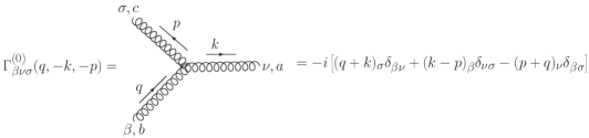
Figure 2: Diagrammatic representation of the free three-gluon vertices $\displaystyle\Gamma^{(0)}_{\mu\alpha\rho}$ and $\displaystyle\Gamma^{(0)}_{\beta\nu\sigma}$. The Lorentz and color indices associated with each gluon momentum $\displaystyle k,q,p$, are denoted as $\displaystyle\mu,\nu,\alpha,\beta,\rho,\sigma$ and $\displaystyle a,b,c$, respectively. The corresponding color factors $\displaystyle f^{abc}$ and $\displaystyle f^{bac}$, accompanying each vertex have been already accounted for in Eqs. (14)-(16) through the identity $\displaystyle f^{abc}f^{bac}=-3$.

With these quantities, the system of tDSE coupled equations for the transversal and longitudinal dressing functions are

$$\displaystyle\frac{1}{Z_{T}}=Z_{3}+\frac{1}{2k^{2}}\frac{3T}{|{\bf k}|\pi}\sum_{i=1}^{2}\frac{D_{2i}}{\left(\omega_{2i}^{T}\right)^{2}}\sum_{m=-\infty}^{\infty}\int d|{\bf q}|\frac{{\bf q}^{3}}{q^{2}}G(q^{2}){\rm e}^{-(\Omega_{mn}^{2}+(|{\bf k}|-|{\bf q}|)^{2})/\left(\omega_{2i}^{T}\right)^{2}}{\cal I}^{(a)}_{1}(\alpha_{i}^{T})+$$

$$\displaystyle\frac{1}{2k^{2}}\frac{3T}{2\pi}\sum_{m}\int d|{\bf q}||{\bf q}|^{2}\int_{-1}^{1}d\xi\,\bigg{\{}{\cal P}^{T}_{\mu\nu}({\bf k})\Gamma_{\mu\alpha\rho}^{(0)}(p,k,-q)\Gamma_{\beta\nu\sigma}^{(0)}(q,-p,-k)\times$$ (42)

$$\displaystyle\frac{1}{q^{2}}\bigg{[}\Delta F_{1}^{T,L}(p_{4},{\bf p}){\cal P}_{\rho\sigma}^{T}({\bf p})+F_{1}^{L}(p_{4},{\bf p}){\cal P}_{\rho\sigma}(p)\bigg{]}\bigg{[}\Delta Z(\Omega_{m},{\bf q}){\cal P}_{\alpha\beta}^{T}({\bf q})+Z_{L}(\Omega_{m},{\bf q}){\cal P}_{\alpha\beta}(q)\bigg{]}\bigg{\}}$$

for the transversal dressing $\displaystyle Z_{T}(k^{2})$ and

$$\displaystyle\frac{1}{Z_{L}}=Z_{3}+\frac{1}{k^{2}}[{\cal P}_{\mu\nu}^{L}(k)]\Sigma^{ghost}_{\mu\nu}(\Omega_{n},{\bf k})+$$ (43)

$$\displaystyle\frac{1}{k^{2}}\frac{3T}{2\pi}\sum_{m}\int d|{\bf q}||{\bf q}|^{2}\int_{-1}^{1}d\xi\,\bigg{\{}{\cal P}_{\mu\nu}^{L}(k)\Gamma_{\mu\alpha\rho}^{(0)}(p,k,-q)\Gamma_{\beta\nu\sigma}(q,-p,-k)\times$$

$$\displaystyle\frac{1}{q^{2}}\bigg{[}\Delta F_{1}^{T,L}(p_{4},{\bf p}){\cal P}_{\rho\sigma}^{T}({\bf p})+F_{1}^{L}(p_{4},{\bf p}){\cal P}_{\rho\sigma}(p)\bigg{]}\bigg{[}\Delta Z(\Omega_{m},{\bf q}){\cal P}_{\alpha\beta}^{T}({\bf q})+Z_{L}(\Omega_{m},{\bf q}){\cal P}_{\alpha\beta}(q)\bigg{]}\bigg{\}},$$

for the longitudinal $\displaystyle Z_{L}(k^{2})$. The explicit expression for $\displaystyle[{\cal P}_{\mu\nu}^{L}(k)]\Sigma^{ghost}_{\mu\nu}(\Omega_{n},{\bf k})]$ in the above equations are given by Eqs. (37)-(40). For the remaining terms, further summations over the Lorentz indices $\displaystyle\mu,\nu,\alpha,\beta,\rho$ and $\displaystyle\sigma$ in the gluon loop, see Fig. 1 and in Eqs. (42) and (43), and subsequent integration over the angle $\displaystyle\xi$ of terms enclosed in curly brackets result in extremely long and cumbersome expressions. The corresponding summation over $\displaystyle\mu,\nu,\alpha,\beta,\rho$ and $\displaystyle\sigma$ procedure and angular integrations over $\displaystyle\xi$, are rather trivial. Nonetheless, because of the cumbersomeness of the final expressions, in the present paper we do not present the resulting system of tDSE explicitly. We note only that the corresponding calculations can be essentially relieved by using a symbol manipulations package, e.g. Maple 18 or Wolfram Mathematica 13. Also note, that the resulting expressions for the gluon loop contain the same, as in the previous case, integrals $\displaystyle{\cal I}^{(a)}_{n}(\alpha)$ and $\displaystyle{\cal K}_{n}(\alpha,b)$, Eqs. (30), now with $\displaystyle n$ from $\displaystyle 0$ to $\displaystyle n=5$.

IV Results and discussions

The resulting system of equations for the ghost and gluon dressing functions, Eqs. (29), (42)-(43) represents the sought rainbow approximation (18)-(20) of the truncated Dyson-Schwinger equations (1)-(2). In Euclidean space, it consists of a system of linear algebraic equations with respect to the Matsubara frequency and one-dimensional integral equations with respect to the three-momentum $\displaystyle|{\bf q}|$. The solution of this system is found numerically by utilisation of an iteration procedure. To this end, the integral equation is replaced by a Gaussian quadrature formula converting the Eqs. (29), (42)-(43) in to a system of algebraic equations with respect to the corresponding Gaussian nodes and Matsubara frequencies, ready for the mentioned numerical procedure. The effective parameters in (21)-(23) generally can be different for the transversal $\displaystyle(T)$ and longitudinal $\displaystyle(L)$ parts. In addition, all parameters, including the renormalization constants, $\displaystyle\tilde{Z}_{3}$ and $\displaystyle Z_{3}$, may depend on the temperature $\displaystyle T$ and Matsubara frequency $\displaystyle\Omega_{n}$, see Ref. Maas:2005hs . However, as it has been observed in Refs. S-XQINprd84 ; Maasprd75 ; lattice1 , at low temperatures the interaction kernel is insensitive to the temperature impact and, as a first approximation, the interaction kernels can be chosen the same as at $\displaystyle T=0$ with $\displaystyle D^{T}=D^{L}$ and $\displaystyle\omega_{i}^{T}=\omega_{i}^{L}$. For larger temperatures such a choice of transversal and longitudinal effective parameters is less justified. In the present paper we use the same values of the effective parameters for longitudinal and transversal parts. The concrete values correspond to the set of parameters previously found by fitting the solution of the tDSE in vacuum, as reported in Ref. ourGlueball : $\displaystyle D_{11}^{T}=D_{11}^{L}=0.462$ GeV², $\displaystyle D_{12}^{T}=D_{12}^{L}=0.116$ GeV², $\displaystyle\omega_{11}^{T}=\omega_{11}^{L}=1.095$ GeV, $\displaystyle\omega_{12}^{T}=\omega_{12}^{L}=2.15$ GeV for the 3-gluon loop, $\displaystyle D_{21}^{T}=D_{11}^{L}=7.7$ GeV², $\displaystyle D_{22}^{T}=D_{22}^{L}=0.25$ GeV², $\displaystyle\omega_{21}^{T}=\omega_{21}^{L}=0.58$ GeV, $\displaystyle\omega_{22}^{T}=\omega_{22}^{L}=4.5$ GeV, for the ghost loop and $\displaystyle\omega_{31}^{T}=\omega_{31}^{L}=0.73$ GeV, $\displaystyle\omega_{32}^{T}=\omega_{32}^{L}=2.16$ GeV $\displaystyle D_{31}^{T}=D_{31}^{L}=0.39\pi$ GeV², $\displaystyle D_{32}^{T}=D_{32}^{L}=0.1\pi$ GeV² for the ghost-gluon loop (cf. the three loops in Fig. 1).

It should be stressed that keeping the effective parameters the same as in vacuum, one can expect reliable solution of the tDSE only at low and moderate temperatures, $\displaystyle T\lesssim 200$ MeV. For higher temperatures, the effective parameters must become $\displaystyle T$- and $\displaystyle n$-dependent (cf. Refs. dor ; S-XQINprd84 for $\displaystyle T$-dependence of the effective parameters and Ref. Maas:2005hs for $\displaystyle n$-dependence of the renormalization constants $\displaystyle Z_{3}$ and $\displaystyle T$-dependence of the coupling constant $\displaystyle g$) and, probably, quite different for the transverse and longitudinal propagators.

We solve the mentioned system of algebraic equation numerically by an iteration procedure. The number of Matsubara frequencies has been fixed in the interval $\displaystyle(-30\,\leq n\,\leq 30$), the Gaussian mesh for the spatial integration on $\displaystyle|{\bf k}|^{2}$ consisted on 72 nodes with the upper limit of integration $\displaystyle|{\bf k}|^{2}\sim 220$ GeV²/c². To obtain more dense Gaussian nodes at low $\displaystyle|{\bf k}|^{2}$, an appropriate mapping has been employed. Notice that, in concrete numerical calculations one can encounter problems evaluating the integrands at $\displaystyle|{\bf q}|\simeq|{\bf k}|$, i.e. at $\displaystyle b=\frac{|{\bf q}|^{2}+|{\bf k}|^{2}}{2|{\bf q}||{\bf k}|}\to 1$ when the integrals $\displaystyle{\cal K}_{n}(a,b)$, Eq. (30), diverge. A careful and scrupulous inspection of the integrands in the vicinity of $\displaystyle b=1$ shows that independently on $\displaystyle n$ the integrals $\displaystyle{\cal K}_{n}(a,b)$ contain the same kind of singularities, viz. singularities of the type $\displaystyle\sim\ln(b-1)+Ei(1,2a)$. They were handled by employing the Taylor expansion of the corresponding expressions about $\displaystyle b=1$ with the conclusion that in the final results there is a full cancelation of all the singularities. Consequently, the final expressions are finite.

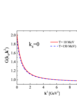
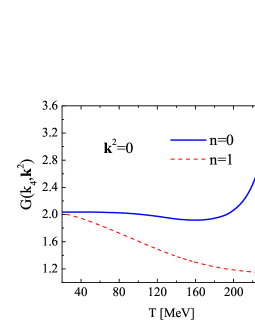
Figure 3: (Color online) The solution of the Dyson-Schwinger equation for the ghost dressing function $\displaystyle G(k_{4},{\bf k}^{2})$. Left panel: dependence on the three-momentum squared $\displaystyle{\bf k}^{2}$ at zero Matsubara frequency, $\displaystyle n=0$, for two values of the temperature $\displaystyle T=10$ MeV (solid curve) and $\displaystyle T=150$ Mev (dashed curve). Right panel: temperature dependence of the dressing function at zero three-momentum $\displaystyle{\bf k}^{2}=0$ and two values of the Mastubara frequency, $\displaystyle n=0$ (solid curve) and $\displaystyle n=1$ (dashed curve).

IV.1 Solution for the the ghost dressing function $\displaystyle G(k_{4},{\bf k}^{2})$

Results of calculations are presented in Fig. 3 where we exhibit the temperature dependence of the ghost dressing function $\displaystyle G(k_{4},{\bf k}^{2})$. Left panel illustrates the dressing function at zero Matsubara frequency, $\displaystyle n=0$, as a function of three-momentum $\displaystyle{\bf k}^{2}$ at two values of the temperature, $\displaystyle T=10$ MeV and $\displaystyle T=150$ MeV. As expected, the temperature dependence is rather weak for all values of $\displaystyle{\bf k}^{2}$, except for the vicinity of very low momenta $\displaystyle{\bf k}^{2}\sim 0$ and is quite similar to the behaviour of $\displaystyle G(k^{2})$ at $\displaystyle T=0$, cf. Ref ourGlueball . In the right panel we present the temperature dependence of the dressing function $\displaystyle G(k_{4},{\bf k}^{2})$ at $\displaystyle{\bf k}^{2}=0$ and two values of the Matsubara frequencies, $\displaystyle n=0$ and $\displaystyle n=1$. Since the fourth component of the ghost momentum strongly depends on the Matsubara frequency, $\displaystyle k_{4}^{2}=[2n\pi T]^{2}$, the dressing function $\displaystyle G(k_{4},0)$ is also quite sensitive to $\displaystyle T$ and $\displaystyle n$. This qualitatively agrees with the lattice QCD calculations reported in Ref. Aouane:2011fv ; Maasprd75 ; lattice1 where it has been found that at low enough three-momenta $\displaystyle|{\bf k}|$ and $\displaystyle T/T_{c}<1.4$ the ghost dressing function $\displaystyle G(k_{4},{\bf k})$ changes rather weakly with the temperature at $\displaystyle k_{4}=0$ and decreases as $\displaystyle k_{4}$ increases. As seen from Fig. 3, the dressing function is basically temperature independent, i.e. $\displaystyle\displaystyle\frac{d}{dT}G(0,0)\sim 0$, up to $\displaystyle T=T_{0}\simeq 150$ MeV. At $\displaystyle T>T_{0}$ the function changes its concavity (the second derivative w.r.t. temperature changes the sign) and sharply increases. In some sense, $\displaystyle T_{0}$ can be considered as the critical point for the temperature dependence of the ghost dressing $\displaystyle G(0,0)$. The ghost dressing for the non-zero Matsubara modes smoothly decreases with $\displaystyle T$ and does not exhibit any irregularities.

IV.2 Solution for the transversal and longitudinal gluon propagators

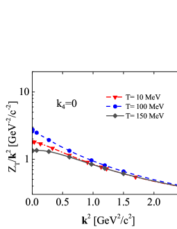
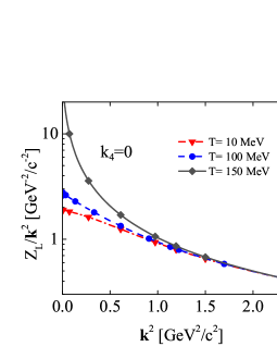
Figure 4: (Color online) Dependence on the three-momentum squared $\displaystyle{\bf k}^{2}$ of the solution of the Dyson-Schwinger equation for the zero Matsubara mode of the transversal $\displaystyle Z_{T}(k_{4},{\bf k}^{2})/k^{2}$ and longitudinal $\displaystyle Z_{L}(k_{4},{\bf k}^{2})/k^{2}$ gluon propagators, left and right panels, respectively. Solid, dashed and dot-dashed curves correspond to $\displaystyle T=150$ MeV, $\displaystyle T=100$ MeV and $\displaystyle T=10$ MeV respectively.

In Figs. 4 and 5 a similar analysis is presented, but now for the gluon propagator. In Fig. 4, the dependence of the propagators for the zero Matsubara mode is displayed as a function of the spatial momentum squared $\displaystyle{\bf k}^{2}$ at several values of the temperature, $\displaystyle T=10$ MeV, $\displaystyle T=100$ MeV and $\displaystyle T=150$ MeV. As in the previous case, the dependence of the transversal, left panel, and longitudinal, right panel, propagators at moderate and large values of $\displaystyle{\bf k}^{2}$ is rather weak. The $\displaystyle T$-dependence of the propagators is more pronounced in the region of low momenta $\displaystyle{\bf k}^{2}$, where transversal and longitudinal propagators manifest quite different behaviour as functions of $\displaystyle T$. While the transversal propagator is not so sensitive to $\displaystyle T$, the longitudinal one sharply increases with increase of $\displaystyle T$. This is more evidently seen in Fig. 5, left panel, where temperature dependence of the Matsubara zero mode is presented at $\displaystyle{\bf k}^{2}\sim 0$. The steep behaviour at $\displaystyle T\sim T_{0}$ of the longitudinal propagator is manifested more distinctly. Moreover, we observed that for larger temperatures $\displaystyle T>T_{0}$, viz. $\displaystyle T\gtrsim 160$ MeV, the iteration procedure does not longer converge and the solution of the tDSE for the gluon propagators disappears. This is a direct indication that our approach with the temperature independent effective parameters cannot be extended to large temperatures.

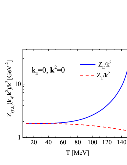
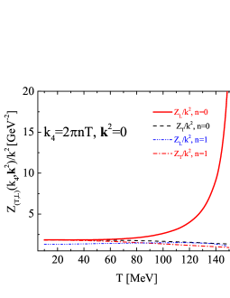
Figure 5: (Color online) The solution of the Dyson-Schwinger equation for the gluon propagators $\displaystyle Z_{L,T}(k_{4},{\bf k}^{2})/k^{2}$. Left panel: temperature dependence of zero Matsubara modes of the propagators at $\displaystyle{\bf k}^{2}=0$. Solid curve corresponds to the longitudinal propagator, the dashed curve is for the transversal one. Right panel: illustration of the temperature dependence of the transversal and longitudinal propagators for zero and non-zero Matsubara modes. Solid and dashed lines are those displayed in the left panel, i.e. for $\displaystyle n=0$. The dot-dot-dashed and dot-dashed lines correspond to longitudinal and transversal propagators at $\displaystyle n=1$, respectively. Note the $\displaystyle log$ scale on the left panel and the linear scale on the right panel.

The right panel in Fig. 5 reflects the $\displaystyle T$-dependence of the gluon propagator at $\displaystyle{\bf k}^{2}=0$ and two values of the Matsubara frequency, $\displaystyle n=0$ and $\displaystyle n=1$. The different behaviour of the longitudinal propagator at moderate and high temperatures is due to vanishing forth component $\displaystyle k_{4}^{2}=0$ for $\displaystyle n=0$ and relatively large values of $\displaystyle k_{4}$, $\displaystyle k_{4}^{2}=4\pi^{2}T^{2}$, for $\displaystyle n=1$. Recall that in the tDS equations with the interaction kernels (21)-(23), the fourth components $\displaystyle k_{4}$ enter as $\displaystyle\exp(-k_{4}^{2}/\omega^{2})$ which essentially affect the values of the corresponding propagators at finite $\displaystyle n$ and large $\displaystyle T$. Since the transverse propagator is less sensitive to the temperature, see left panel in Fig. 5, the dependence on the Matsubara modes is not so strong. This is in a fairly good qualitative agreement with the results obtained for the interval temperature interval ($\displaystyle 0\leq T\leq 150$ MeV) within the FRG framework (see Refs. Dupuis:2020fhh ; DressingPawlowsky ; PawlowskyFRG ; MaasPhysReport and references therein quoted) and within the lattice QCD simulations Aouane:2011fv ; Ilgenfritz:2017kkp ; lattice1 , where a noticeable sensitivity of the longitudinal component of the gluon propagator with respect to the deconfining phase transition has been observed. This effect easily see from the behaviour of the electric screening mass

$$m_{L}=\left.\sqrt{\frac{k^{2}}{Z_{L}(k4,|{\bf k}|)}}\ \right|_{k^{2}\to 0}.$$ (44)

Figure 6 illustrates the temperature dependence of $\displaystyle m_{L}$. It can be seen that the screening mass is a decreasing function of $\displaystyle T$ in the whole, available in the present analysis, temperature range $\displaystyle T<T_{0}$ in an agreement with SU(2) and SU(3) lattice calculations lattice1 . For larger temperature the lattice calculations predict a drastic increase of $\displaystyle m_{L}$ at $\displaystyle T>T_{c}$, where $\displaystyle T_{c}$ is a critical temperature for phase transitions (e.g. for chiral phase transition $\displaystyle T_{c}=154\pm 9$ MeV critical1 , whereas the SU(3) pure Yang-Mills theory predicts a first order transition at the critical temperature $\displaystyle T_{c}\sim 270$ MeV critical ).

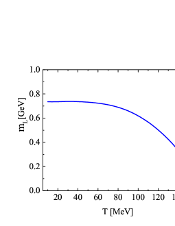
Figure 6: (Color online) The electric screening mass, Eq. (44), as function of the temperature $\displaystyle T$.

We reiterate that our simplified approach with fixed parameters from vacuum cannot be reliably applied at larger temperatures, $\displaystyle T\gtrsim 160$ MeV, and a comparison with FRG and/or lattice QCD approaches at higher temperatures is therefore hindered. An analysis of the possible temperature dependence of the effective parameters of the approach will be presented elsewhere.

V Summary

In summary, we solve numerically the system of truncated gluon-ghost Dyson-Schwinger equations within the rainbow approximation at finite temperatures within the framework of the Matsubara imaginary-time formalism. The effective parameters of the interaction kernels have been considered as temperature independent and taken from the previous fit of the gluon and ghost propagators to the SU(2) lattice QCD results in vacuum. We argue that for the zero-Matsubara frequency, $\displaystyle n=0$, the dependence of the dressing functions on the three-momentum squared $\displaystyle{\bf k}^{2}$ is not sensitive to the temperature $\displaystyle T$ in almost the whole range of $\displaystyle{\bf k}^{2}$. Contrarily, a strong dependence on $\displaystyle n$ and $\displaystyle T$ has been found at the origin, $\displaystyle{\bf k}^{2}=0$. We found that, with effective parameters fixed from vacuum calculations the iteration procedure of solving the tDSE does not converge at large enough temperatures, $\displaystyle T>T_{0}$, where $\displaystyle T_{0}\sim 150-160$ MeV. In the vicinity of $\displaystyle T_{0}$, the longitudinal gluon propagator sharply increases, whereas the transversal one does not exhibit irregularities. It means that, if one searches for some gluon phase transitions, then the most appropriate quantity to study is the temperature dependence of the longitudinal propagators. The presented investigations can be considered as a first step in further, more reliable, analysis of the $\displaystyle T$-dependence of gluon and ghosts propagators. The obtained solution of the tDSE can be directly implemented in to the Bethe–Salpeter equations to perform studies of behaviour glueballs as two-gluon bound states in hot and dense matter.

VI Acknowledgments

A bulk of numerical calculations have been performed on the basis of the HybriLIT heterogeneous computing platform govorun (supercomputer ”Govorun”, LIT, JINR).

References

- (1) V. G. Bornyakov, E.-M. Ilgenfritz, C. Litwinski, M. Müller-Preussker and V. K. Mitrjushkin, Landau gauge ghost propagator and running coupling in SU(2) lattice gauge theory, Phys. Rev. D 92, 074505 (2015).
- (2) V. G. Bornyakov, V. K. Mitrjushkin and M. Müller-Preussker, SU(2) lattice gluon propagator: continuum limit, finite-volume effects and infrared mass scale , Phys. Rev. D81, 054503 (2010).
- (3) R. Aouane, V. G. Bornyakov, E. M. Ilgenfritz, V. K. Mitrjushkin, M. Muller-Preussker and A. Sternbeck, Landau gauge gluon and ghost propagators at finite temperature from quenched lattice QCD, Phys. Rev. D 85, 034501 (2012).
- (4) E. M. Ilgenfritz, J. M. Pawlowski, A. Rothkopf and A. Trunin, Finite temperature gluon spectral functions from lattice QCD, Eur. Phys. J. C 78, no.2, 127 (2018).
- (5) P. O. Bowman, U. M. Heller, D. B. Leinweber, M. B. Parappilly, A. Sternbeck, L. von Smekal, A. G. Williams and J. Zhang, Scaling behavior and positivity violation of the gluon propagator in full QCD, Phys. Rev. D 76, 094505 (2007).
- (6) P. O. Bowman, U. M. Heller, D. B. Leinweber, M.B. Parappilly amd A. G. Williams, Unquenched Gluon Propagator in Landau Gauge, Phys. Rev. D 70, 034509 (2004).
- (7) M. Albanese et al. [Ape Collaboration], Glueball Masses and the Loop Loop Correlation Functions, Phys. Lett. B 197, 400 (1987).
- (8) Y. Chen, A. Alexandru, S. Dong, T. Draper, I. Horvath et al. Glueball spectrum and matrix elements on anisotropic lattices, Phys. Rev. D 73, 014516 (2006).
- (9) C. J. Morningstar and M. J. Peardon, The Glueball spectrum from an anisotropic lattice study, Phys. Rev. D 60, 034509 (1999).
- (10) N. Dupuis, L. Canet, A. Eichhorn, W. Metzner, J. M. Pawlowski, M. Tissier and N. Wschebor, The nonperturbative functional renormalization group and its applications, Phys. Rept. 910, 1-114 (2021)
- (11) A.K. Cyrol, M. Mitter, J.M. Pawlowski, N. Strodthoff, Non-perturbative finite temperature Yang-Mills theory, Phys. Rev. D 97, 054015 (2018).
- (12) M. A. Shifman, A. I. Vainshtein, and V. I. Zakharov, QCD and Resonance Physics. Theoretical Foundations, Nucl. Phys. B 147, 385 (1979).
- (13) E. V. Shuryak, The Role of Instantons in Quantum Chromodynamics. 2. Hadronic Structure, Nucl. Phys. B203, 116 (1982).
- (14) C. Fischer, QCD at finite temperature and chemical potential from Dyson-Schwiger equations, Progr. Part. Nucl. Phys., 105, 1 (2019).
- (15) A. Maas, Gauge bosons at zero and finite temperature, Phys. Repts., 524, 203 (2013).
- (16) A. Das ”Finite Temperature Field Theory”, World Scientific Publishing , 1997.
- (17) R. Alkofer, P. Watson, H. Weigel, Mesons in a Poincare covariant Bethe-Salpeter approach, Phys. Rev. D 65, 094026 (2002).
- (18) C. Roberts, V. Bnagwat, A. Holl, S. Wringht, Aspects of Hadron Physics, Eur. Phys. J. ST 140, 53 (2007).
- (19) P. Maris, P. C. Tandy, Bethe-Salpeter study of vector meson masses and decay constants, Phys. Rev. C 60, 055214 (1999).
- (20) S. M. Dorkin, L. P. Kaptari and B. Kämpfer, Accounting for the analytical properties of the quark propagator from the Dyson-Schwinger equation, Phys. Rev. C 91, 055201 (2015).
- (21) Si-xue, Lei Chang, Yu-xin Liu,C. Roberts, Quark spectrfal density and strongly-coupled quark-gluon plasma, Phys. Rev. D 84, 014017 (2011).
- (22) M. Blank, A. Krassnigg, The QCD transition temeprature in a Dyson-Schwinger-equation context, Phys. Rev. D 82, 034006 (2010).
- (23) S. Dorkin, L.P. Kaptari, B. Kämpfer, Pseudo-scalar bound states at finite temperatures, Few Body Syst. 60, 20 (2019).
- (24) S. Dorkin, M. Viebach, L. Kaptari, B. Kämpfer, Extending the truncated Dyson-Schwinger equatin to finite temperatures, J. Mod. Phys. 7, 2071 (2016).
- (25) L. von Smekal, A. Hauck, R. Alkofer, A solution to coupled Dyson-Schwinger equations for gluons and ghosts in Landau gauge, Ann. Phys. 267, 1 (1998).
- (26) B. Gruter, R. Alkofer, A. Maas, J. Wambach, Temperature Dependence of Gluon and Ghost Propagators in Landau-Gauge Yang–Mills Theory below the Phase Transition, Eur.Phys.J. C 42 (2005) 109-118;
- (27) C.W. Bernard, Feynman rules for gauge theories at finite temperature, Phys. Rev. D9 (1974) 3312.
- (28) D.J. Gross, R.D. Pisarski, J.W. Gibbs, G. Yaffe, QCD and instantons at finite temperature, Rev. Mod. Phys. 53 (1981) 43.
- (29) Varouzhan Baluni, Non-Abehan gauge theories of Fermi systems: Quantum-chromodynamic theory of highly condensed matter, Phys. Rev. D 17 (1978) 202.
- (30) C. S. Fischer, P. Watson and W. Cassing, Probing unquenching effects in the gluon polarisation in light mesons, Phys. Rev. D 72, 094025 (2005).
- (31) L.P. Kaptari, B. Kämpfer, Mass spectrum of pseudo-scalar glueballs from a Bethe-Salpeter approach with the rainbow-ladder-truncation, Few. Body Syst. 61, 28 (2020).
- (32) L.P. Kaptari, B. Kämpfer, Modeling the gluon and ghost propagators in Landau gauge by truncated Dyson-Schwinger equations, Eur. Phys. J. Plus 134 (2019) 383.
- (33) A. Hauck, L. von Smekal and R. Alkofer, Solving the Gluon Dyson-Schwinger Equation in the Mandelstam Approximation, Comput. Phys. Commun. 112, 149 (1998).
- (34) S. Mandelstam, Approximation scheme for quantum chromodynamics, Phys. Rev. D 20, 3223 (1979).
- (35) K. Buttner and M.R. Pennington, Infrared behavior of the gluon propagator: Confining of confined? Phys. Rev. D 52, 5220 (1995).
- (36) D. Atkinson and J. C. R. Bloch, Running coupling in nonperturbative QCD. 1. Bare vertices and y-max approximation, Phys. Rev. D 58, 094036 (1998).
- (37) L. von Smekal, A. Hauck and R. Alkofer, The Infrared Behavior of Gluon and Ghost Propagators in Landau Gauge QCD, Phys. Rev. Lett. 79, 3591 (1997).
- (38) R. Alkofer and L. von Smekal, The Infrared behavior of QCD Green’s functions: Confinement dynamical symmetry breaking, and hadrons as relativistic bound states, Phys. Rept. 353, 281 (2001).
- (39) A. Maas, J. Wambach and R. Alkofer, The High-temperature phase of Landau-gauge Yang-Mills theory, Eur. Phys. J. C 42, 93 (2005).
- (40) A. Cucchieri, A. Maas, T. Mendes, Infrared properties of propagators in Landau gauge pure Yang-Mills theory at finite temperature Phys. Rev. D 75, 07600 (2007).
- (41) C. S. Fischer, A. Maas, and J. A. Müller, Chiral and deconfinement transition from correlation functions: SU(2) vs. SU(3), Eur. Phys. J. C68, 165 (2010).
- (42) Wei-jie Fu, J.M. Pawlowski, F. Rennecke, QCD phase structure at finite temperature and density, Phys. Rev. D 101, 054032 (2020).
- (43) Ph. Boucaud, J. P. Leroy, A. Le Yaouanc, J. Micheli, O. Pene and J. Rodriguez-Quintero, The Infrared Behaviour of the Pure Yang-Mills Green Functions, Few-Body Syst. 53, 387 (2012).
- (44) A. Bazavov, T. Bhattacharya, M. Cheng, C. DeTar, H.-T. Ding et al., Chiral and deconfinement aspects of the QCD transition, Phys. Rev. D 85, (2012) 054503.
- (45) P.J. Silva, O. Oliveira, P. Bicudo, N. Cardoso, Gluon screening mass at finite temperature from the Landau gauge gluon propagator in lattice QCD, Phys. Rev. D 89 (2014) 074503.
- (46) Gh. Adam, M. Bashashin, D. Belyakov, M. Kirakosyan et al. IT-ecosystem of the HybriLIT heterogeneous platform for high-performance computing and training of IT-specialists. The 8th International Conference ”Distributed Computing and Grid-technologies in Science and Education” (GRID 2018), Dubna, Russia, September 10-14, 2018, CEUR-WS.org/Vol-2267.