Path separation of dissipation-corrected targeted molecular dynamics simulations of protein-ligand unbinding

Abstract

Protein-ligand (un)binding simulations are a recent focus of biased molecular dynamics simulations. Such binding and unbinding can occur via different pathways in and out of a binding site. We here present a theoretical framework how to compute kinetics along separate paths and to combine the path-specific rates into global binding and unbinding rates for comparison with experiment. Using dissipation-corrected targeted molecular dynamics in combination with temperature-boosted Langevin equation simulations [Nat. Commun. 11, 2918 (2020)] applied to a two-dimensional model and the trypsin-benzamidine complex as test systems, we assess the robustness of the procedure and discuss aspects of its practical applicability to predict multisecond kinetics of complex biomolecular systems.

I Introduction

Reaction paths (or pathways) constitute a central concept to describe biophysical processes such as protein folding, allostery, and the binding and unbinding of biomolecular complexes.Chipot07 When we consider the free energy landscape $\Delta G({\boldsymbol{x}})$ along a (in general multidimensional) reaction coordinate ${\boldsymbol{x}}$ describing such a process, the minima correspond to metastable states reflecting the stationary distribution, while the valleys and saddle points connecting the minima account for the flux and thus the transfer rates between the states.Wales03 The connection between two minima is in general not unique, i.e., various folding or unbinding pathways can exist. Hence biophysical processes can be described via path integrals,Faccioli06 sampling schemes such as transition path sampling,Dellago16 or weighed ensemble methods.Zuckerman17 The knowledge of reaction paths is also useful to construct biasing coordinates, along which the sampling of rare transition events can be enhanced. Capelli19 ; Capelli19a ; Rydzewski19 ; Bianciotto21 ; NunesAlves21 ; Henin22

In this work, we further exploit the concept of reaction paths to facilitate the general applicability of dissipation-corrected targeted molecular dynamics (dcTMD),Wolf18 ; Wolf20 ; Post22 a recently developed method to calculate slow (say, second-long) biomolecular kinetics from atomistic simulations.Tiwary15 ; Plattner15 ; Teo16 Combining enhanced sampling techniques with Langevin modeling, dcTMD applies a constant velocity constraint to drive an atomistic system from an initial state into a target state, say, the bound and unbound states of a protein-ligand complex. To extract the equilibrium free energy from these nonequilibrium simulations, dcTMD exploits Jarzynski’s identityJarzynski97 ; Hendrix01 ; Dellago14

$$\beta\Delta G=-\ln\left<\mathrm{e}^{-\beta W}\right>,$$ (1)

which estimates the free energy difference $\Delta G$ between the two states from the amount of work $W$ done on the system to enforce the nonequilibrium process. Here $\left<\ldots\right>$ denotes an ensemble average over statistically independent nonequilibrium simulations starting from a common equilibrium state, and $\beta=1/\mathrm{k}_{\mathrm{B}}T$ is the inverse temperature. To avoid problems associated with the poor convergence behavior of the exponential average,Ytreberg04 ; Echeverria12 we may exploit the second-order cumulant expansion of Jarzynski’s identity,

$$\Delta G\approx\left<W\right>-\frac{\beta}{2}\left<\delta W^{2}\right>,$$ (2)

where the first term represents the averaged external work, while the second term (with $\delta W=W-\left<W\right>$) corresponds to the mean dissipated work $\left<W_{\rm diss}\right>$ of the process (and explains the name ’dissipation-corrected’ TMD). Since the knowledge of $W_{\rm diss}$ allows us to calculate the friction coefficient ${\it{\Gamma}}$, in a second step the equilibrium dynamics of the process can be studied by propagating a Langevin equation, which is based on the free energy $\Delta G$ and the friction ${\it{\Gamma}}$ obtained from dcTMD.Wolf20

If the distribution of the external work $W$ is well approximated by a Gaussian, the cumulant approximation in Eq. (2) is known to become exact. Since this approximation is indispensable for the efficient treatment of large molecular systems, the assumption of a normal work distribution is in fact the main (and formally only) condition underlying dcTMD. We expect such a distribution in the limit of slow pulling, where the response of the system is linear and the work is given as sum of many independent contributions, Hendrix01 ; Wolf18 as required by the central limit theorem.Billingsley95 In practice, though, this consideration is mainly of academic interest, because the computational effort is inversely proportional to the pulling velocity. By extending the argument to independent contributions in space, Post et al.Post22 argued that a Gaussian work distribution is also found for fluids. On the other hand, the assumption was shown to break down in the case of ligand-protein dissociation processes that provide several exit pathways of the ligandWolf20 or ion diffusion through a membrane channel coupled to a conformational change of the protein.Jager22

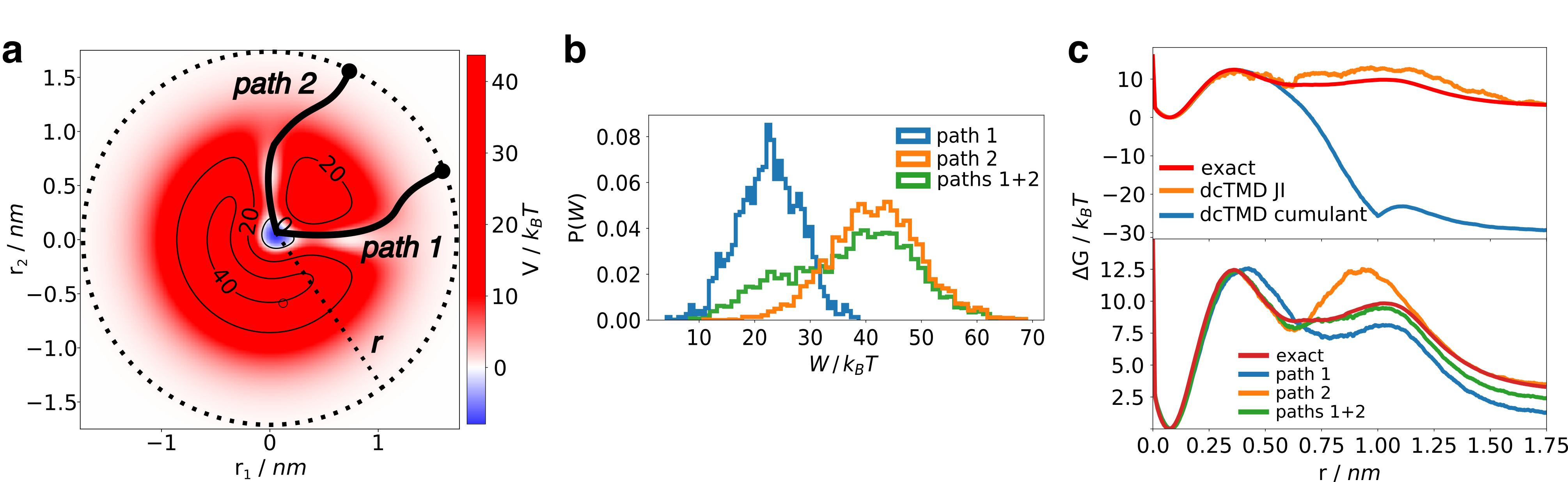
Figure 1: 2D model of ligand-protein dissociation, illustrating the separation of the total reaction flux into two paths 1 and 2. (a) Potential energy landscape $V(r,\theta)$, where the radial coordinate $r$ corresponds to the ligand-protein distance and the angle $\theta$ accounts for the direction of the process. (b) Total work distribution (green) compared to the distributions from the individual paths 1 (blue) and 2 (orange), obtained at $r=r_{D}$ from the dcTMD simulations. (c) Comparison of free energy profiles $\Delta G(r)$. (Top) Exact $\Delta G(r)$ (red) as calculated from Eq. (I), compared to dcTMD simulations using Jarzynski’s identity [Eq. (1), in orange] and its cumulant approximation [Eq. (2), in blue], where we averaged over 5000 dcTMD runs. (Bottom) Free energy profiles for the individual paths 1 (blue) and 2 (orange), and resulting dcTMD estimates of the total free energy (green) compared to the exact result (red).

To explain the origin of this breakdown, we consider a minimal model of ligand-protein dissociation, given by a two-dimensional (2D) potential energy landscape $V(r,\theta)$ and corresponding friction profile ${\it{\Gamma}}(r,\theta)$ (see the Supplementary Material and Fig. S1 for details). As shown in Fig. 1a, the initial bound state is located at the origin ($r\!=\!0$), and the dissociated state is reached via external pulling along the radial coordinate $r$ to $r_{D}=1.75$ nm. While in most directions (defined by the angle $\theta$), the ligand encounters high energy barriers mimicking the steric hindrance of the surrounding protein, two well-separated paths (’1’ and ’2’) of relatively low energy exist, along which dissociation may occur. In general, these paths will exhibit different free energy curves as well as different friction factors, but both end at the same energy, accounting for the dissociated state.

Aiming to model the dissociation process via dcTMD, we pull the ligand along the radial coordinate $r$ accounting for the ligand-protein distance, giving rise to the free energy profile

$$\beta\Delta G(r) =-\ln\left[\rmintop\nolimits_{0}^{\infty}\!\!r^{\prime}\,\mathrm{d}r^{\prime}\delta(r-r^{\prime})\,\rmintop\nolimits_{0}^{2\pi}\mathrm{d}\theta\;\mathrm{e}^{-\beta V(r^{\prime},\theta)}\,\right]$$

$$=-\ln\left[\rmintop\nolimits_{0}^{2\pi}\!\!\mathrm{d}\theta\;\mathrm{e}^{-\beta V(r,\theta)}\right]-\ln r,$$ (3)

where the factor $-\ln r$ represents the configurational entropy arising from the Jacobian of the projection. Doudou09 As shown in Fig. 1c, the exact free energy $\Delta G(r)$ calculated from Eq. (I) exhibits (by design) two maxima at $r\sim\,0.36$ and $1.03$ nm, before the ligand dissociates for large $r$. Performing dcTMD simulations in combination with Jarzynski’s identity (1), the reference results for $\Delta G(r)$ are only accurately reproduced for small $r$, but deteriorate at larger distances due to sampling problems. Invoking the cumulant approximation, on the other hand, only the first barrier is reproduced, while the free energy goes to nonphysically low values ($\sim-30\,\mathrm{k}_{\mathrm{B}}T$) for longer ligand-protein distances. Figure 1b reveals the reason for this drastic breakdown of the cumulant approximation by clearly showing a non-Gaussian shape of the corresponding work distribution, which leads to an overestimation of the variance of the work and thus also of the dissipated work.

To present a remedy for this problem, we note that in our simple model the dissociation can occur exclusively through either path 1 or 2. Hence we may consider trajectories following one of these paths separately, and calculate the work distribution associated with this path. To define a simple separatrix of the two paths, we use the diagonal $r_{1}=r_{2}$ in Fig. 1a for 0.44 nm $\leq r\leq$ 0.88 nm. Interestingly, Fig. 1b reveals that the work distributions of the individual paths are both well approximated by a Gaussian, although of different means and widths (for an illustration of the sampling per path, see Figs. S1d-f). Adding these distributions (weighted by the probability that the corresponding path is taken), we by design recover the total work distribution, which readily explains its bimodal appearance. Most importantly, the finding of normal work distributions for each path suggests that we may apply the cumulant approximation for each path separately, in order to obtain the correct free energy profiles for the two paths, as is shown in Fig. 1c. The theory of path separation including the calculation of observables from various paths is a central goal of this work and will be developed in Sec. II D.

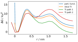
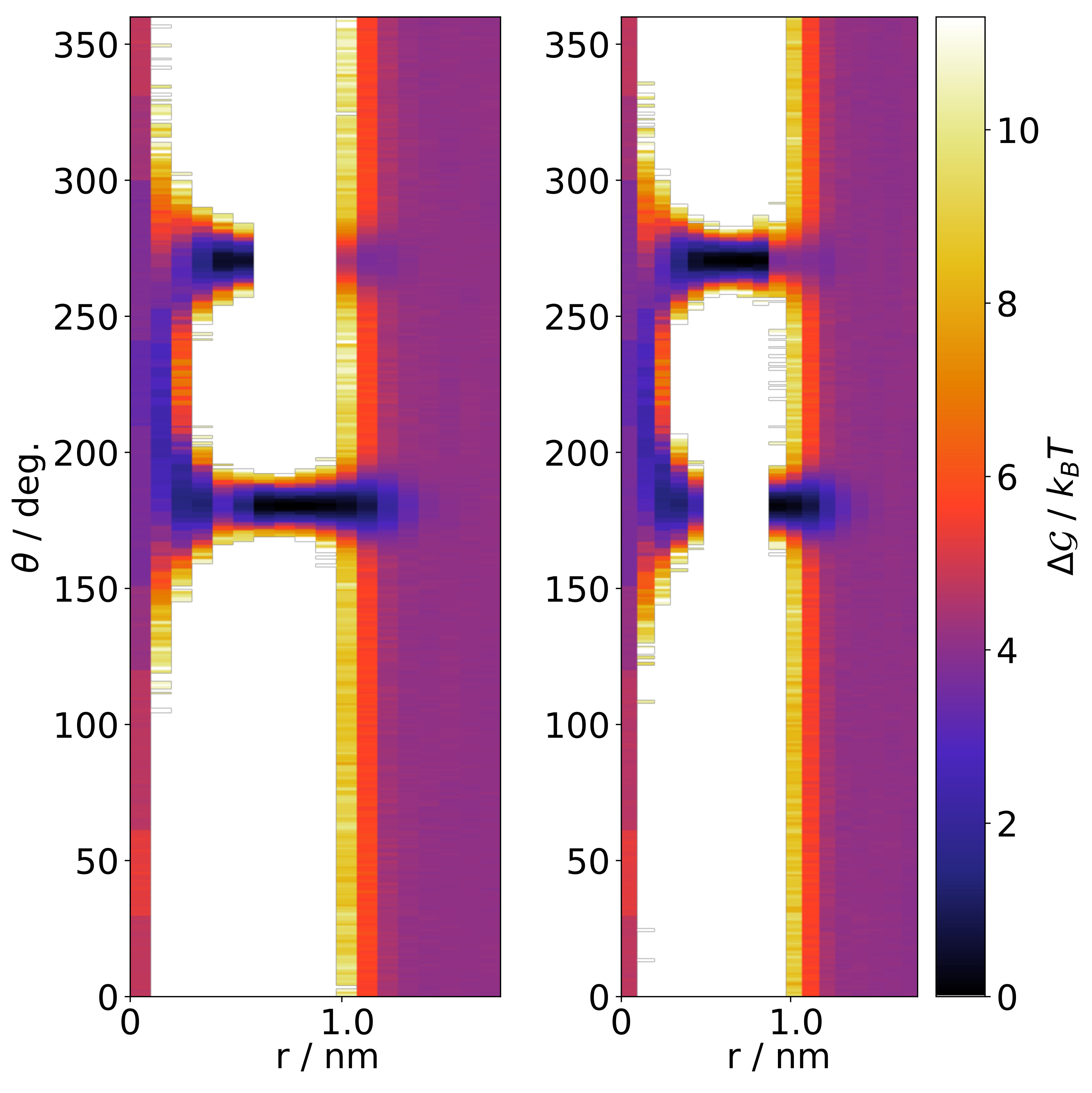
Figure S2: Thermodynamic integration study of the 2D model of ligand-protein dissociation. (Left) Free energy profiles obtained for various TI protocols: In “ideal TI”, we sampled over all angles for each $r$. Apart from numerical issues, this result should therefore agree with the exact result obtained from the partition function. Moreover, two Monte Carlo TI calculations are shown, which were started at path 1 and 2, respectively. Since TI is in principle exact, these curve should also coincide with the exact result. However, both calculations fail, due to jumps between the two path. (Right) 2D representation of the energy landscape of the model, reflecting the jumps of the Monte Carlo TI calculations starting at path 1 ($\sim 180^{\circ}$) and 2 ($\sim 270^{\circ}$). Note that for each value of $r$, the Monte Carlo moves can only go vertically.

While the discussion above seems to concern a technical problem of dcTMD, we note that it represents in fact a quite general issue. It occurs whenever we perform enhanced sampling along a 1D biasing coordinate, although the considered process in fact takes place on a multidimensional energy landscape with several reaction channels. As an illustration, Fig. S2 shows various thermodynamic integration protocols to calculate the free energy profile $\Delta G(r)$ of the 2D model. Although thermodynamic integration is in principle exact, it is found to typically fail in this example. This is a consequence of incomplete sampling of the two paths by the biasing due to the absence of jumps over the path-separating energy barrier, which should also occur for other 1D biasing techniques such as umbrella sampling.

Motivated by this simple example, in this work we present general theoretical considerations under which conditions a separation of the total reaction flux in several pathways is possible, in the sense that it ensures the validity of the cumulant approximation and thus the applicability of dcTMD. We also discuss the question which paths are most important (i.e., exhibits the highest reaction rates), and which paths can be safely neglected. In practical calculations, the definition and detection of paths represent a nontrivial issue. To this end, we consider nonequilibrium principal component analysis Post19 as a generic dimensionality reduction approach, which allows to determine and characterize various paths in a low-dimensional space. Employing the trypsin-benzamidine complex Guillain70 ; Marquart83 as a well-established model problem to test enhanced sampling techniques,Buch11 ; Plattner15 ; Tiwary15 ; Teo16 ; Votapka17 ; Betz19 the performance and the potential of the proposed path separation scheme is discussed.

II Theory

II.1 Dissipation-corrected targeted molecular dynamics

For further reference, we first briefly summarize the theoretical foundation of dcTMD, which was given in Refs. Wolf18, ; Wolf20, ; Post22, . To pull two molecules apart (e.g., protein and ligand), TMD as developed by Schlitter et al. Schlitter94 uses a constraint force $f$ that results in a moving distance constraint $x=x_{0}+vt$ with a constant velocity $v$. Pulling from $x_{0}$ to $x$, the mean external work performed on the system is given by

$$\left<W(x)\right>=\rmintop\nolimits_{x_{0}}^{x}\mathrm{d}x^{\prime}\left<f(x^{\prime})\right>\,,$$ (4)

where $\left<\ldots\right>$ again denotes the average over all nonequilibrium trajectories. Evaluating the second cumulant of the work in Eq. (2), we obtain the dissipated workWolf18

$$\left<W_{\rm diss}(x)\right> =\frac{\beta}{2}\rmintop\nolimits_{x_{0}}^{x}\!\mathrm{d}x^{\prime}\rmintop\nolimits_{x_{0}}^{x}\!\mathrm{d}x^{\prime\prime}\left<\delta f(x^{\prime})\delta f(x^{\prime\prime})\right>\,,$$ (5)

which is defined via the autocorrelation function of the constraint force $\delta f=f-\left<f\right>$.

Exploiting that the cumulant approximation neglects higher orders of the force autocorrelation function and due the simplification arising from the constraint $x=x_{0}+vt$, we can –without further approximation– derive a generalized Langevin equation of the nonequilibrium process,Post22

$$m\ddot{x}(t)=-\frac{\partial G}{\partial x}-\rmintop\nolimits^{t}_{0}\!\mathrm{d}\tau K(t,\tau)\,\dot{x}(\tau)+\eta(t)+f(t)=0\,,$$ (6)

which includes the mean force $-\partial G/\partial x$, a non-Markovian friction force with memory function $K(t,\tau)$, a stochastic force $\eta(t)$ due to the associated colored noise with zero mean, and the external pulling force $f(t)$. The memory kernel is given by the autocorrelation function of the constraint force,

$$K(t_{2},t_{1})=\beta\left<\delta f(t_{2})\delta f(t_{1})\right>\,.$$ (7)

It obeys the fluctuation dissipation theorem

$$K(t_{2},t_{1})=\beta\left<\eta(t_{2})\eta(t_{1})\right>,$$ (8)

which states that non-white noise $\eta$ causes a finite decay time of the memory kernel $K$. Nevertheless, by using $\dot{x}(\tau)=v$, Eq. (6) can be written in the form of a Markovian Langevin equation

$$m\ddot{x}(t)=-\frac{\partial G}{\partial x}-{\it{\Gamma}}(x(t))\,\dot{x}(t)+\eta(t)+f(t)=0,$$ (9)

although the noise $\eta(t)$ is not delta-correlated due to Eq. (8). Here

$${\it{\Gamma}}(x)=\rmintop\nolimits_{0}^{t(x)}\mathrm{d}t^{\prime}K(t,t^{\prime})$$ (10)

represents the position-dependent friction ${\it{\Gamma}}(x)$ associated with the pulling process. Employing Eq. (5), the friction can also be directly calculated from the dissipated work viaPost22

$${\it{\Gamma}}(x)=\frac{\beta}{2\,v}\,\frac{\partial}{\partial x}\left<\delta W^{2}(x)\right>,$$ (11)

which is numerically advantageous compared to Eq. (10), as it avoids the computationally expensive calculation of autocorrelation functions. Data analysis was performed using Python packages NumPy,Harris20 SciPy,Virtanen20 and Pandas.McKinney10 Matplotlibhunter07 and Gnuplotgnuplot were used for generating plots. Calculations with the 2D model were carried out using a Jupyter notebook.Kluyver16

II.2 Calculation of reaction rates

The Langevin model may be used to discuss the nonequilibrium process in terms of the memory function $K(t_{2},t_{1})$ and the associated friction ${\it{\Gamma}}(x)$, which both are directly obtained from dcTMD. What is more, we can employ the free energy $\Delta G(x)$ and the friction ${\it{\Gamma}}(x)$ from dcTMD to simulate the unbiased dynamics via the free Langevin equation [Eq. (48) with $f=0$]. While Jarzynski’s identity [Eq. (1)] states that this is correct for the free energy, the friction determined by dcTMD in general depends on the pulling velocity $v$, see Ref. Post22, . Since this velocity dependence affects the overall transition rates (typically by a factor of $\sim 2$) clearly less than errors in the estimate of the energy barrier, the usage of dcTMD friction factors in equilibrium Langevin simulations nevertheless represents a promising strategy to estimate transition rates of slow processes.Wolf20

The theoretical formulation of dcTMD given above can be nicely illustrated by a simple model proposed by Zwanzig,Zwanzig73 which couples a general 1D system (in general nonlinearly) to a harmonic bath. In the unbiased case (with constraint force $f=0$), it is well established that the model gives rise to an exact general Langevin equation as in Eq. (48). As shown in the Appendix, the formulation readily generalizes to the case of constrained dynamics used in dcTMD, revealing that both biased and unbiased dynamics can be described by the same Langevin model. Moreover, we derive explicit expressions for the resulting external force $f(t)$ and the associated work $W$. Starting from a Boltzmann distribution (as required for Jarzynski’s identity), in particular, we obtain a Gaussian distribution of the work, which renders the cumulant approximation exact.

When we intend to model very slow processes such as ligand-protein dissociation that can take seconds to hours, there is one more practical issue to overcome. That is, since the numerical integration of the Langevin equation typically require time steps of a few femtoseconds, we would need to propagate Eq. (48) for $\gtrsim 100\cdot 10^{15}$ steps to sufficiently sample a process occurring on a timescale of seconds. As a remedy, we employ the method of “$T$-boosting” which exploits the fact that temperature is the driving force of the Langevin dynamics.Wolf20 That is, when we consider a process described by a transition rate $k$ and increase the temperature from $T_{1}$ to $T_{2}$, the corresponding rates $k_{1}$ and $k_{2}$ are related by the Kramers-type expression

$$k_{2}=k_{1}\mathrm{e}^{-\Delta G^{\neq}(1/(\mathrm{k}_{\mathrm{B}}T_{2})-1/(\mathrm{k}_{\mathrm{B}}T_{1}))}\,,$$ (12)

where $\Delta G^{\neq}$ denotes the transition state energy of the process. Hence, by increasing the temperature we also increase the number $n$ of observed transition events according to $n_{2}/n_{1}=k_{2}/k_{1}$. Unlike methods like temperature-accelerated MD,Sorensen00 where $\Delta G(x)$ is first calculated at a high temperature and subsequently rescaled to a desired low temperature (whereupon $\Delta G(x)$ in general changes), $T$-boosting does not need to assume that $\Delta G(x)$ is independent of $T$, because by using dcTMD we calculate $\Delta G(x)$ right away at the desired temperature. See Ref. Wolf20, for a discussion of the performance of $T$-boosting for the trypsin-benzamidine complex.

II.3 Validity of the cumulant approximation

Since the main presumption of dcTMD is that the distribution of the work $W$ resembles a Gaussian to justify the cumulant approximation (2), it is important to study the validity of this assumption. To this end, we integrate Eq. (48) from the initial position $x_{0}$ to the end position $x$, yielding

$$W(x)=\Delta G(x)+v\rmintop\nolimits_{x_{0}}^{x}\!\!\mathrm{d}x^{\prime}{\it{\Gamma}}(x^{\prime})-\rmintop\nolimits_{x_{0}}^{x}\!\!\mathrm{d}x^{\prime}\eta(x^{\prime}),$$ (13)

where we defined $\eta(t)=\eta((x\!-\!x_{0})/v)\equiv\eta(x)$. Upon averaging, the stochastic force term cancels out (since $\left<\eta(x)\right>\!=\!0$), which again leads to the relation $\Delta G=\left<W\right>-\left<W_{\rm diss}\right>$ discussed above. On the other hand, when we consider the work $W$ associated with a single trajectory, we find that the first two terms on the right-hand-side of Eq. (13) are identical for all trajectories, due to the constraint $x=x_{0}+vt$. Hence the distribution of the work, $P(W)$, is completely determined by the distribution $P(\delta W_{\rm diss})$ of the integrated noise $\delta W_{\rm diss}(x)\equiv\rmintop\nolimits_{x_{0}}^{x}\!\!\mathrm{d}x^{\prime}\eta(x^{\prime})$. In other words, if $P(\delta W_{\rm diss})$ is normal distributed, so is the work distribution $P(W)$.

Given as a sum of many small noise increments $\eta(x)$, the central limit theorem generally assures that $P(\delta W_{\rm diss})$ is a normal distribution. Importantly, this holds even if the noise $\eta$ arising in the Langevin equation is not Gaussian distributed; only the integrated noise $\delta W_{\rm diss}$ needs to be Gaussian. Moreover this conclusion holds for position-dependent noise and friction, as long as the noise integral is not dominated by some singularly high noise increments, for which the central limit theorem breaks down. Billingsley95 Given these conditions and the special case that the problem can be properly described by a single reaction coordinate $x$, we therefore expect a Gaussian work distribution and thus the validity of the cumulant approximation.

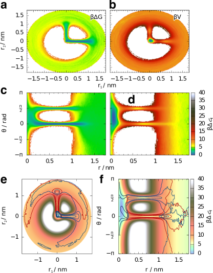
Figure S3: Sampling of the 2D potential energy landscape in nonequilibrium pulling. (a) Distribution in $(r_{1},r_{2})$ of all pulled trajectories as a biased density $\mathcal{V}$, estimated by a histogram. (b) Corresponding reweighed potential $V$ using Eq. (11) of Ref. Post19, . (c) Same data but projected onto $(r,\theta)$ coordinates. (d) Corresponding reweighed density. (e) Biased trajectories separated by pathways superimposed on unbiased potential in the $(r_{1},r_{2})$ plane, visualized by isolines of same biased density. (f) Same data but in $(r,\theta)$.

The situation becomes considerably more involved, when the system cannot be described by a single reaction coordinate $x$, but requires another (in general multidimensional) coordinate ${\boldsymbol{y}}$ for an appropriate description. Assuming for simplicity a 2D model, this means that the system is pulled along coordinate $x$, but additionally can freely evolve along coordinate $y$. Potential implications of the additional degree of freedom on the resulting work distribution have been illustrated in Fig. 1 for a simple model problem, where the motion along $y=\theta$ gives rise to a splitting of the 2D energy landscape into two 1D pathways (See also Fig. S3). While the work distributions of the individual paths are well approximated by a Gaussian, their means and widths are different, such that the sum of the Gaussians exhibits a bimodal appearance. As a consequence, we cannot simply apply the cumulant approximation to the full problem, but need to resort to a treatment of the individual paths.

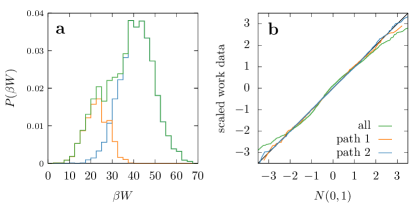
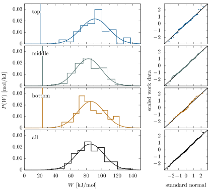
Figure S4: Normality test of $P(W)$ obtained for (top panels) the 2D model and (bottom panels) for trypsin. (a) $P(W)$ for complete and path-separated trajectory sets. (b) Normality tests for these sets. The complete trajectory set displays clear deviations in the tails from the ideal diagonal, while the path-separated sets display better agreement. (Bottom panels) Results for trypsin, showing (left) $P(W)$ for complete and path-separated trajectory sets and (right) normality tests for these sets. Both the path-separated the complete trajectory sets display rather good agreement with a normal distribution.

We note in passing that in practice it is not obvious how to test the Gaussianity of the work distribution, in order to ensure that the cumulant approximation works. While well-established normality tests exist, Henderson06 we found their results rather inconclusive for the problem at hand, especially for the small number of trajectories that are available for atomistic protein-ligand models. As a qualitative means to study the shape of the work distribution $P(W)$, especially its tail for low $W$, we may compare $P(W)$ to a normal distribution whose mean and variance matches the sampled mean and variance. In practice, we compare the points of the computed work to the quantiles of the corresponding normal distribution, such that the deviations reveal a non-Gaussian shape. This has the advantage that the comparison explicitly shows all data points and does not depend on the choice of bins. The test is demonstrated in Fig. S4 for the 2D model, which exhibits deviations from normality in the full trajectory set that become resolved in the path-separated sets.

II.4 Path separation

To study under which conditions a separation of the total reaction flux into several non-interacting pathways is possible and helpful for practical calculations, we now present a mathematical description of the path separation scheme discussed above. To this end, we again assume that the considered process is well represented as a function of the pulling coordinate $x$ and of a further coordinate ${\boldsymbol{y}}$, along which the system can evolve freely. Given the resulting free energy landscape $\Delta G(x,{\boldsymbol{y}})$, we wish to define a reaction path $k$ as a class of similar trajectories $\left(x,{\boldsymbol{y}}\right)(t)$, whose distribution can be characterized by a 1D free energy curve $\Delta G_{k}(x)$, which describes this specific path from an initial (e.g., bound) state to a final (e.g., unbound) state. This definition corresponds to the assumption of distinct ”valleys” in $\Delta G(x,{\boldsymbol{y}})$ connecting $x_{0}$ and $x_{\rm end}$. For simplicity, we for now assume that trajectories of different paths should be mutually exclusive, i.e., the paths should not overlap. As the latter condition may be difficult to satisfy in practice, we will discuss in Sec. II.7 a procedure to relax this condition.

Given the free energy landscapes $\Delta G(x,{\boldsymbol{y}})$ and $\Delta G(x)$, we first introduce the probabilities

$$P(x,{\boldsymbol{y}}) =\mathrm{e}^{-\beta\Delta G(x,{\boldsymbol{y}})}/Z,$$ (14)

$$P(x) =\mathrm{e}^{-\beta\Delta G(x)}/Z=\rmintop\nolimits\!\!\mathrm{d}{\boldsymbol{y}}\,\mathrm{e}^{-\beta\Delta G(x,{\boldsymbol{y}})}/Z,$$ (15)

$$Z =\rmintop\nolimits\!\!\mathrm{d}x\,\mathrm{e}^{-\beta\Delta G(x)}=\rmintop\nolimits\!\!\mathrm{d}x\!\rmintop\nolimits\!\!\mathrm{d}{\boldsymbol{y}}\,\mathrm{e}^{-\beta\Delta G(x,{\boldsymbol{y}})}.$$ (16)

To partition the probability $P(x)$ into paths labeled by $k\!=\!1,\ldots,K$, we define regions ${\boldsymbol{Y}}_{k}(x)$ of the free energy landscape $\Delta G(x,{\boldsymbol{y}})$, such that they only include trajectories of path $k$, i.e., ${\boldsymbol{Y}}_{k}(x)=\{{\boldsymbol{y}}\,|\,(x,{\boldsymbol{y}})\in\text{path}\,k\}$. This allows us to write

$$P(x) =\sum_{k}P(x,k),$$ (17)

$$P(x,k) =\frac{1}{Z}\rmintop\nolimits_{{\boldsymbol{y}}\in{\boldsymbol{Y}}_{k}(x)}\!\!\!\!\!\!\!\!\!\!\!\!\!\!\!\mathrm{d}{\boldsymbol{y}}\,\mathrm{e}^{-\beta\Delta G(x,{\boldsymbol{y}})},$$ (18)

where $P(x,k)$ represents the joint probability to be on path $k$ and at position $x$. Additional regions of the free energy landscape $\Delta G(x,{\boldsymbol{y}})$ not covered by the reaction paths (such as hardly accessible high-energy regions) can formally be included via additional terms of the sum, but are not of interest here, as they have a negligible impact on the integral in Eq. (17). Alternatively, we may write

$$P(x,k)=p_{k}P(x|k),$$ (19)

where $p_{k}$ is the probability to be on path $k$ and $P(x|k)$ is the resulting conditional probability to be at position $x$ if path $k$ is followed. In this way, specified by adding the subscript or superscript “eq”, we may interpret the partitioning in Eqs. (17) and (19) in terms of the free energy as

$$P_{\rm eq}(x,k)\equiv p_{k}^{\rm eq}\,\mathrm{e}^{-\beta\Delta G_{k}(x)}/Z,$$ (20)

which yields the equilibrium path probabilities $p_{k}^{\rm eq}$ and path free energy curves $\Delta G_{k}(x)$. Both quantities are needed when we want to calculate the reaction rates of the system via a Langevin model as will be described in Sec. II.5.

Since we typically cannot calculate these quantities directly (due to the MD simulation time limits mentioned before), we perform nonequilibrium dcTMD simulations. Let us assume that we have in total $N$ nonequilibrium trajectories labeled by $n\!=\!1,\ldots,N$, which are divided into the $K$ different paths, each containing $N_{k}$ trajectories labeled by $n_{k}\!=\!1,\ldots,N_{k}$. Due to the initial preparation of the system and the nature of the paths, each path occurs in the dcTMD simulations with an observed probability $p_{k}^{\rm neq}=N_{k}/N$. Expressing the ensemble average $\left<\ldots\right>$ as a sum over all nonequilibrium trajectories $n$ with work $W_{n}(x)$, we obtain from Jarzynski’s identity [Eq. (1)]

$$\mathrm{e}^{-\beta\Delta G(x)} =\frac{1}{N}\sum_{n=1}^{N}\mathrm{e}^{-\beta W_{n}(x)}=\sum_{k=1}^{K}\frac{N_{k}}{N}\frac{1}{N_{k}}\!\sum_{n_{k}=1}^{N_{k}}\mathrm{e}^{-\beta W_{n_{k}}\!(x)}$$

$$=\sum_{k}p_{k}^{\rm neq}\left<\mathrm{e}^{-\beta W(x)}\right>_{k}\equiv\sum_{k}p_{k}^{\rm neq}\,\mathrm{e}^{-\beta\Delta\mathcal{G}_{k}(x)}\,,$$

$$\equiv Z\sum_{k}P_{\rm neq}(x,k),$$ (21)

where $\left<\ldots\right>_{k}$ denotes the average over all trajectories of path $k$, and $\Delta\mathcal{G}_{k}(x)$ represents the energy profile along this path. Note that the latter can per se not be identified with the free energy curves $\Delta G_{k}(x)$ in Eq. (20), because the path energy curves $\Delta\mathcal{G}_{k}(x)$ as well as the path probabilities $p_{k}^{\rm neq}$ are nonequilibrium quantities that depend on the protocol of the dcTMD simulations such as the pulling velocity $v$.

Since Jarzynski’s identity can be generalizedPost19 to estimate the free energy landscape $\Delta G(x,{\boldsymbol{y}})$, we may project the corresponding joint probability $P(x,{\boldsymbol{y}})$ onto each path $k$ along coordinate $x$, yielding $P_{\rm neq}(x,k)=P_{\rm eq}(x,k)$. This equivalence can be used to calculate the equilibrium path probabilities $p_{k}^{\rm eq}$ from the nonequilibrium simulations via

$$p_{k}^{\rm eq} \equiv\rmintop\nolimits\mathrm{d}xP_{\rm eq}(x,k)$$ (22)

$$=\frac{p_{k}^{\rm neq}}{Z}\rmintop\nolimits\mathrm{d}x\,\mathrm{e}^{-\beta\Delta\mathcal{G}_{k}(x)},$$ (23)

where the partition function

$$Z=\sum_{k}p_{k}^{\rm neq}\rmintop\nolimits\!\!\mathrm{d}x\,\mathrm{e}^{-\beta\Delta\mathcal{G}_{k}(x)}$$ (24)

is obtained from the the path estimates in Eq. (II.4). (To derive Eq. (23), we used that $Z=\rmintop\nolimits\mathrm{d}x\,\mathrm{e}^{-\beta\Delta G(x)}=\rmintop\nolimits\mathrm{d}x\,\mathrm{e}^{-\beta\Delta G_{k}(x)}$ for any path $k$, which is a consequence of the normalization condition $\rmintop\nolimits\mathrm{d}x\,P(x|k)=1$.) Moreover, the equivalence shows that the free energy curves $\Delta G_{k}(x)$ in Eq. (II.4) and the corresponding nonequilibrium energy curves $\Delta\mathcal{G}_{k}(x)$ in Eq. (23) simply differ by a constant shift of the energy

$$\Delta G_{k}(x)=\Delta\mathcal{G}_{k}(x)+\beta^{-1}\ln\left(p^{\text{eq}}_{k}/p^{\text{neq}}_{k}\right)\,.$$ (25)

As a consequence, both energy curves give rise to the same mean force $f_{\rm PMF}=-\partial G/\partial x$ in Langevin equation (48), and can therefore both be considered as potentials of mean force.

Just as for the general Jarzynski identity (1), the direct evaluation of the exponential average $\left<\mathrm{e}^{-\beta W(x)}\right>_{k}$ of path $k$ in Eq. (II.4) is numerically cumbersome. However, when we assume that the work associated with each individual path is normal distributed, the potential of mean force along path $k$ can be calculated using the cumulant approximation,

$$\Delta\mathcal{G}_{k}(x)\approx\left<W(x)\right>_{k}-\frac{\beta}{2}\left<\delta W^{2}(x)\right>_{k},$$ (26)

which was the main motivation to perform the path separation in the first place.

II.5 Path importance

When studying ligand-protein dissociation, a natural indicator for the importance of a reaction path is the reaction rate at equilibrium. This is because the total dissociation rate $k_{\rm tot}$ is given as the sum over all equilibrium rates contributing to the considered process. Assuming that path $k$ occurs in an equilibrium simulation with probability $p^{\text{eq}}_{k}$, the total rate can be written as

$$k_{\rm tot}=\sum_{k}p^{\text{eq}}_{k}k_{k}\,,$$ (27)

where $k_{k}$ is the rate associated with the path. We note that Eq. (27) corresponds to the well-known sumLogan96 $k_{\rm tot}=\sum_{k}\tilde{k}_{k}$ of weighted first-order reaction rates $\tilde{k}_{k}=p^{\text{eq}}_{k}k_{k}$. The weights $p^{\text{eq}}_{k}$ account for the correct partitioning of the process into paths, because the calculation of a rate along a single path does not include the possibility to switch between various paths. Since a single path with an extraordinary high rate may completely dominate the reaction, it is clearly of interest to identify the most important pathways of a reaction. In this way, several paths of similar importance may exist and therefore all contribute to $k_{\rm tot}$.

As an illustrative example, we again consider the simple model discussed in Fig. 1, which shows two reaction paths ($k=1,2$) with nonequilibrium energy curves $\Delta\mathcal{G}_{k}(r)$. Using these curves and the associated path probabilities $p_{1}^{\text{neq}}\approx 0.81$ and $p_{2}^{\text{neq}}\approx 0.19$ from dcTMD, Fig. 1c shows that the correct overall free energy $\Delta G(r)$ is indeed nicely recovered from Eq. (II.4). (As discussed in Sec. II.7, we exclude dcTMD trajectories that initially cross between paths 1 and 2 (about 4 %) from the analysis.) The corresponding equilibrium path probabilities $p_{1}^{\text{eq}}\approx 0.79$ and $p_{2}^{\text{eq}}\approx 0.21$ obtained from Eq. (23) are quite similar to the nonequilibrium results, which indicates that $x$ is a suitable reaction coordinate.

To obtain the dissociation and association rates of the model, we perform $10\times 1$ ms-long unbiased Langevin simulations [Eq. (48) with $f\!=\!0$] independently for each 1D path (see the Supplementary Material for details). As shown in Tab. 1, the two paths differ in their importance for both binding and unbinding. While path 2 exhibits larger rates for both processes, path 1 is accessed in 80 % of all attempts, such that path 1 has the largest impact on the overall binding and unbinding rate. Using Eq. (27), we also calculated the total dissociation and association rates, i.e., averaged over the two paths. This is of particular interest, because for the simple 2D model the total rate can also be directly calculated by performing Langevin simulations on the ’full-dimensional’ potential energy landscape, i.e., without performing a separation into 1D paths (see Fig. S3 for details). Table 1 shows perfect agreement of path-based rates and 2D results for dissociation, while the association rates are found to differ by 14 %.

	$p^{\text{neq}}_{k}$	$p^{\text{eq}}_{k}$	$k_{\rm off}$ (ms-1)	$k_{\rm on}$ (ms-1)
path 1	$0.81\pm 0.01$	$0.79\pm 0.01$	$16\pm 2$	$210\pm 20$
path 2	$0.19\pm 0.01$	$0.21\pm 0.01$	$55\pm 3$	$230\pm 10$
total	–	–	$24\pm 2$	$220\pm 10$
total (2D)	–	–	$24\pm 2$	$190\pm 10$

Table 1: Dissociation ($k_{\rm off}$) and association ($k_{\rm on}$) rates of paths $k=1,\,2$ of the 2D model in Fig. 1, obtained from unbiased Langevin simulations using the path free energy profiles $\mathcal{G}_{k}(x)$. Furthermore, nonequilibrium ($p^{\text{neq}}_{k}$) and equilibrium ($p^{\text{eq}}_{k}$) weights of the two paths are given, which are used to obtain the total rates via Eq. (27). For comparison, total rates are also calculated from Langevin simulations on the 2D potential energy landscape. Values in brackets denote the standard error of the mean. The error of the total rates from Eq. (27) is obtained from error propagation.

The above example demonstrates that even for a apparently simple model problem, the interpretation of the various pathways contributing to the reaction rate may be not straightforward. Rather than resorting to approximate theories such as Kramers’ relation (which, e.g., assumes a single barrier of parabolic shape and constant friction), we therefore recommend the calculation of reaction rates via the numerical propagation of the unbiased Langevin equation.

II.6 Path detection

In our introductory example shown in Fig. 1, the two paths of the model are readily identified via visual inspection of the 2D potential energy landscape. When we consider an all-atom MD simulation of a protein-ligand complex, however, this is typically not possible because the trajectories evolve in a $3N\!-\!6$-dimensional space of the $N$ atoms of the complex. Hence in a first step, we need to employ some dimensionality reduction approach to identify collective variables that appropriately describe the unbinding dynamics in a low-dimensional space,Noe17 ; Sittel18 and allow to cluster the unbinding trajectories into different reaction pathways.

While various techniques to identify ligand unbinding paths have been suggested, Votapka17 ; Capelli19 ; Rydzewski19 ; NunesAlves21 ; Bianciotto21 here we employ a principal component analysis (PCA) of protein-ligand contacts, Ernst15 which assumes that these contacts are suitable features to represent the unbinding process. Considering an equilibrium MD simulation with coordinates ${\boldsymbol{q}}=\{q_{i}\}$, the basic idea is to construct the covariance matrix

$$\sigma_{ij}^{\rm eq}=\left<\delta q_{i}\delta q_{j}\right>_{\rm eq},$$ (28)

where $\delta q_{i}\!=\!q_{i}\!-\!\left<q_{i}\right>_{\rm eq}$. PCA represents a linear transformation that diagonalizes $\sigma$ and thus removes the instantaneous linear correlations among the variables. Ordering the eigenvalues of eigenvectors ${\boldsymbol{e}}_{n}^{\rm eq}$ decreasingly, the first principal components $V_{n}^{\rm eq}={\boldsymbol{e}}_{n}^{\rm eq}\cdot{\boldsymbol{\delta q}}$ account for the directions of largest variance of the data, and are therefore often used as collective variables.Amadei93 ; Altis08

When we consider dcTMD simulations that enforce the unbinding of a complex along the pulling coordinate $x$, we wish to identify the directions of largest variance of the dcTMD data, in order to separate the unbinding trajectories into different paths. Hence we calculate the covariances directly from the dcTMD simulations, and average over $x$ to obtain the nonequilibrium covariance matrixPost19

$$\sigma^{\rm neq}_{ij}=\frac{1}{x_{\rm end}-x_{0}}\rmintop\nolimits_{x_{0}}^{x_{\rm end}}\mathrm{d}x\,\left<\delta q_{i}(x)\delta q_{j}(x)\right>_{{\rm neq}}.$$ (29)

This leads to principal components $V^{\rm neq}_{n}$ that map out an energy landscape $\Delta\mathcal{G}$ associated with the nonequilibrium distribution generated by dcTMD. In practice, this simply means to perform a PCA of the concatenated TMD trajectories. Performing the PCA on contact distances, the first principal component by design correlates with the pulling coordinate. This connection may not be given if other input features, such as dihedral angles, are employed. In this case, we can consider the content of eigenvectors to identify their respective dynamics in Cartesian space.

Note that this nonequilibrium PCA is well defined, because the nonequilibrium principal components are related to their equilibrium counterparts via Jarzynski’s identity. That is, when we replace the equilibrium average in Eq. (28) by a Jarzynski-type average over the nonequilibrium data, we obtainPost19 ; Hummer01

$$\sigma_{ij}^{\rm eq} =\frac{\rmintop\nolimits\!\!\mathrm{d}x\left<\delta q_{i}(x)\delta q_{j}(x)\,\mathrm{e}^{-\beta W(x)}\right>_{\rm neq}}{\rmintop\nolimits\!\!\mathrm{d}x^{\prime}\left<\mathrm{e}^{-\beta W(x^{\prime})}\right>_{\rm neq}}\,,$$ (30)

which is an equilibrium covariance matrix constructed via the reweighting of the nonequilibrium data. We note that the dimensionality reduction of nonequilibrium dcTMD data proposed in Ref. Post19, is not restricted to PCA, but may as well be used in combination with nonlinear or machine learning empowered approaches.Rohrdanz13 ; Glielmo21

II.7 Applicability and practical considerations

When we apply the above introduced path separation approach to all-atom MD simulations of ligand unbinding, various general as well as practical problems may arise. As so often, the key issue is the appropriate choice of coordinates to define the free energy landscape $\Delta G(x,{\boldsymbol{y}})$ of the system. Most importantly, the pulling coordinate $x$ should represent a suitable 1D reaction coordinate of the unbiased system, such that equilibrium and nonequilibrium path weights are similar. The collective variables $\{y_{j}\}={\boldsymbol{y}}$, on the other hand, should allow for a low-dimensional representation of the free motion of the system “around” coordinate $x$. In particular, the purpose of coordinate ${\boldsymbol{y}}$ is to facilitate the detection of reaction pathways. As discussed above, a straightforward choice for ${\boldsymbol{y}}$ are the first principal components of a PCA of protein-ligand contacts. Representing an internal coordinate system of the protein-ligand complex, these coordinates may describe unbinding routes through 3D space along which the ligand can minimize steric clashes with the protein, thereby managing to find a low-energy exit path from the binding pocket. Other candidates for ${\boldsymbol{y}}$ are protein backbone dihedral angles (in case that the unbinding is connected to a protein conformational change Amaral17 ; Jager22 ) and intra-ligand hydrogen bonds (whose change affect the ligand’s conformational flexibility Bray22 ).

Given these coordinates, the subsequent clustering of unbinding trajectories into distinct reaction paths is based on the assumption that these paths are well separated on the free energy landscape $\Delta G(x,{\boldsymbol{y}})$. If the energy landscape between two paths is flat, however, trajectories may cross between the paths and thus hamper a clear path separation. Even for the simple 2D model discussed in Fig. 1, we find crossing trajectories at the beginning of both paths, which constitute $\sim 4\,$% of all performed simulations (see Fig. S1c). In principle, we could cut crossing trajectories into segments that are attributed to different paths. However, similarity measures between crossing and other trajectories are typically inconclusive, and the calculation of path energy curves [Eq. (26)] using a varying number of trajectories for each position $x$ turns out to be quite inefficient. Considering an atomistic description of ligand unbinding, on the other hand, crossings between various exit paths may naturally occur also during the unbinding process. In the limiting case that the free energy landscape is overall flat, most trajectories will cross and a path separation ansatz does not make sense from the outset. On the other hand, if only some smaller part of the trajectories cross, and if we assume that they do not change the path energy curves, we may remove these trajectories from the analysis.

Proceeding with more practical aspects of path separation, we note that the occurrence of crossing trajectories also depends sensitively on the pulling velocity $v$. In general, we want to choose $v$ low enough to ensure that motions described by coordinate ${\boldsymbol{y}}$ have sufficient time to relax. This corresponds to a slow adiabatic change,Servantie03 which leaves the system virtually at equilibrium at all positions $x$. On the other hand, if $v$ is chosen too slow, the constraint can artificially facilitate transitions over barriers along ${\boldsymbol{y}}$; a process that might not happen in the unconstrained case. In this way, low pulling velocities may lead to an increase of crossing trajectories. To find a balance between these conflicting conditions, in practice we will try to find a sweet spot of the pulling velocity, which typically is around 1 m/s for ligand-protein complexes (see Fig. S4 of Ref. Wolf20, ). We note in passing that fast pulling velocities may also result in a jamming of the ligand in an unfavorable position of the binding pocket, which in consequence leads to a sharp peak of the constraint force when unbinding is enforced. Since this effect would not occur at equilibrium, however, jammed trajectories can be safely neglected.

III Application: The Trypsin-Benzamidine Complex

The inhibitor benzamidine bound to trypsinGuillain70 ; Marquart83 is a well-established model problem to test enhanced sampling techniques.Buch11 ; Plattner15 ; Tiwary15 ; Teo16 ; Votapka17 ; Betz19 As the unbinding process is well characterized and occurs on a millisecond timescale, Guillain70 the complex represents an ideal system to study the virtues and shortcomings of the path separation scheme.

III.1 Computational details

MD and dcTMD simulations of the trypsin-benzamidin complex were described in detail in Ref. Wolf20, . In brief, all simulations were performed using Gromacs 2018 (Ref. Abraham15, ) in combination with the Amber99SB force field Hornak06 ; Best09 for the protein. Ligand parameters were obtained from AntechamberWang06 with GAFF atomic parameters.Wang04 Atomic charges were obtained from quantum calculations at the HF/6-31G* level using OrcaNeese12 followed by RESP charge calculations in Multiwfn.Lu12 The TIP3P modelJorgensen83 was used for the solvent water, and the 1.7 Å crystal structureMarquart83 (PDB 3PTB) as starting condition. dcTMD calculations were carried out using the PULL code implemented in Gromacs. The constraint was defined via the distance between the centers of mass of the heavy atoms of benzamidine and the C_α atoms of the central $\beta$-sheet of the protein. Sampling from an equilibrium simulation at 290 K, 400 statistically independent starting points were obtained, for which dcTMD simulations were performed using a pulling velocity $v=1$ m/s. Using 400 simulations, the least populated path is taken by 52 simulations, which is typically suitable to obtain sufficiently accurate PMF and path weight estimates.Wolf18 ; Wolf20 The accumulated simulation time of 0.8 $\mu$s required a total wall clock time of 640 hours on a workstation with an Intel i7-3930K processor and a NVIDIA GeForce GTX 670.

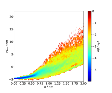
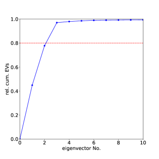
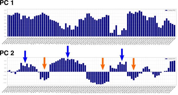
Figure S5: Results from a contact PCA, obtained for the trypsin-benzamidine complex. (Top left) Correlation between pulling distance $x$ and 1^st principal component. (Top right) Cumulative fluctuations obtained from the principal components. The first two components already explain 78% of the variance of the data. (Bottom) Eigenvector contributions from single contacts. Residues defining pathways displayed in Fig. 2 of the main text are indicated by accordingly colored arrows.

For path separation we employed a nonequilibrium PCAPost19 on protein-ligand contacts, see Sec. II.6. Concatenating all 400 dcTMD runs into a single pseudo-trajectory, we determined all residues that exhibit a minimal distance $\leq 4.5$ Å between the heavy atoms of benzamidine and the protein.Ernst15 Using these contacts and the fastpca program,Sittel17 the nonequilibrium covariance matrix [Eq. (29)] and the associated principal components were obtained (Fig. S5). For the calculation of binding and unbinding rates, free energy and friction fields obtained from dcTMD were employed to run unbiased Langevin equation simulations, see the Supplementary Material for details. To enhance the sampling, we employ the $T$-boosting technique described in Sec. II.2, using five independent simulations of 200 $\mu s$ length each at 13 different temperatures between 380 and 900 K.

III.2 Results and Discussion

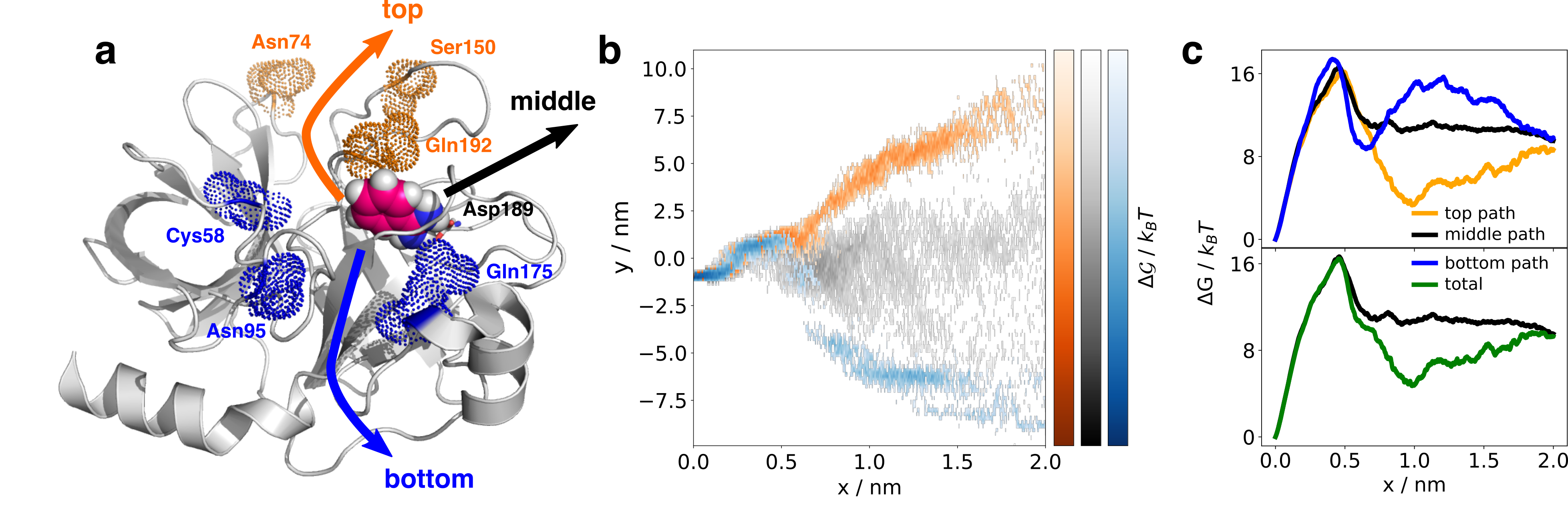
Figure 2: dcTMD simulations of the trypsin-benzamidine complex. (a) Structure of trypsin (PDB ID 3PTB)Marquart83 showing the protein surface as cartoon (grey), the ligand benzamidine as van der Waals spheres (magenta), and residue Asp189 in sticks. Colored arrows indicate the direction of the three observed paths, which are characterized by equally colored residues displayed as volumes. (b) Nonequilibrium energy landscape $\Delta\mathcal{G}(x,y)$ indicating the three paths, represented as a function of the pulling coordinate $x$ and the second principal component $y$ of a PCA on ligand-protein contacts. (c) Free energy profiles along $x$ obtained by dcTMD. (Top) Path-specific free energy curves $\Delta G_{k}(x)$ with color code according to pathway taken. (Bottom) Comparison of the free energy profiles of the middle path and the combined paths [Eq. (II.4)].

Figure 2 displays the structure of trypsin and indicates the direction of the three observed dissociation paths of benzamidine by colored arrows. Using the same colors, we also show the resulting nonequilibrium energy landscape $\Delta\mathcal{G}(x,y)$, represented as a function of the pulling coordinate $x$ and the second principal component $y$ of a contact PCA. We note that coordinate $x$ is highly correlated with the first principal component (Fig. S5), which therefore could also be used instead of $x$. On the other hand, coordinate $y$ encodes the dissociation path by reporting on the direction along which benzamidine moves over the protein surface after unbinding. As shown in Fig. S5, the 2D representation already explains 78% of the total variance of the unbinding process.

All unbinding simulations start with a common rupture of the benzamidine-Asp189 salt bridge at $x\sim\,0.5$ nm, which allows the ligand to exit the binding pocket.Wolf20 Subsequently, the diffusion of benzamidine away from the binding site funnel is found to follow different routes along the protein surface. As can be derived from the contributions of individual contacts to $y$ in Fig. S5, the ”top” pathway (i.e., corresponding to high values in $y$) leads to a motion along residues Asn74, Ser150 and Gln192, which are highlighted in orange in Fig. 2. The ”bottom” pathway, on the other hand, corresponds to diffusion close to residues Cys58, Asn95 and Glu175 highlighted in blue. Finally, the ”middle” pathway describes unbinding directly into the bulk water. For all paths, $P(W)$ exhibits a normal distribution, see Fig. S4. However, we note that the shifts of the mean $\left<W\right>$ are small compared to the distributions’ widths, rendering this type of analysis difficult.

Figure 2c shows the resulting free energy profiles $\Delta G_{k}(x)$ of the three paths. In line with the 2D energy landscape, all paths show the same increase of the free energy until the transition state at $x\sim\,0.5\,$nm, which reflects the rupture of the benzamidine-Asp189 salt bridge. Following this main energy barrier, the free energy of the ”top” pathway drops to a subsequent deep minimum at $x\sim\,1.0\,$nm, which is indicative of an unspecific binding site on the surface of the protein involving Tyr151. This binding site was also discussed in Ref. Buch11, , therein named S3. The ”middle” path, on the other hand, rapidly levels off to the free energy value of the unbound state. This agrees with the path leading directly into the bulk water, which was also found in Ref. Wu16, . The ”bottom” pathway exhibits a second minimum at $x\sim\,0.7\,$nm, followed by a 2^nd energy barrier at $x\sim\,1.2\,$nm. This unspecific binding site close to, e.g., Glu175 has also been observed in Ref. Buch11, (therein named S2). Moreover, our transition state agrees with the findings of Ref. Tiwary15, .

path	$p^{\text{neq}}_{k}$	$p^{\text{eq}}_{k}$	$k_{\rm off}(10^{2}$/s)	$k_{\rm on}(10^{5}$/sM)	$K_{\rm D}(10^{-5}$ M)
unsep.	—	—	$20\pm 3$	$21\pm 2$	$100\pm 20$
top	0.23	0.29	$7.9\pm 1.2$	$0.42\pm 0.03$	—
middle	0.57	0.52	$8.0\pm 1.0$	$78\pm 4$	—
bottom	0.20	0.19	$3.2\pm 0.4$	$45\pm 3$	—
total	—	—	$7.1\pm 0.9$	$49\pm 3$	$15\pm 3$
exp.Guillain70	—	—	$6$	$290$	$2$

Table 2: Dissociation and association rates of the unseparated data and the three paths found for the trypsin-benzamidine complex (Fig. 2), along with their nonequilibrium and equilibrium weights. The resulting total rates [Eq. (27)] as well as the equilibrium dissociation constant $K_{\rm D}$ are compared to experimental data.Guillain70 Values in brackets denote the fitting error from $T$-boostingWolf20 for path-specific rates, and results from error propagation for total rates.

Let us now turn to the analysis of the kinetics predicted for the various pathways. Comprising the nonequilibrium and equilibrium weights as well as the dissociation and association rates of the three paths, Tab. 2 reveals that the ”middle” path is the most populated (148 trajectories out of 400), while the two other paths each have less than 40 % population. We additionally encounter a significant number of crossing trajectories (139 out of 400), which were discarded in the analysis. Apart from being the most accessed path, the middle pathway provides also the fastest way in and out of the protein, and results in rates that are surprisingly similar to the experimental findings.Guillain70 For these reasons, we focused in our previous workWolf20 on the main path and did not further investigate the remaining paths. In the present more elaborated study, however, we find that the unbinding rate $k_{\rm off}$ is nearly identical for the three paths. This may be related to the fact that all paths coincide on the 1D and 2D energy landscapes in Fig. 2 until the transition state. Concerning the binding process, we find that the top path is by two orders of magnitude slower than the other two paths, which is due to the deep minimum of the free energy at $x\approx 1.0$ nm.

When we finally compare to experiment, we find that the calculated total unbinding rates reproduces the observed rate within its error margin, while the binding rate is underestimated by a factor of $\sim$6. Consequently, the equilibrium dissociation constant $K_{\rm D}=k_{\rm off}/k_{\rm on}$ is overestimated by a factor of $\sim$6 as well. We note that this corresponds to an underestimation of the standard free energy of binding $\Delta G^{0}=-\mathrm{k}_{\mathrm{B}}T\ln K_{\rm D}$ by $\sim$1.8 $\mathrm{k}_{\mathrm{B}}T$, which is well below the mean error ($\sim$3 $\mathrm{k}_{\mathrm{B}}T$) of current prediction methods of absolute binding free energy.Fu22 Furthermore, we note that ignoring the existence of paths and employing the free energy and friction profiles from all 400 simulations will cause rate estimates to deteriorate by a factor of $\sim$3 and the dissociation constant by a factor of $\sim$7 (see Tab. II). This comparatively small offset comes from the fact that the friction overestimation artifact in trypsin is particularly small around the sweet spot velocity of 1 m/s.

IV Conclusions

When we employ dcTMD pulling simulations to calculate free energy profiles and reaction rates of slow processes, the practical implementation of the method rests on the cumulant approximation of Jarzynski’s identity [Eq. (2)], which is valid given a normal distribution of the work done on the system. By exploiting the central limit theorem, this is found to be the case if the integrated noise $\rmintop\nolimits\!\mathrm{d}t\,\eta(t)$ associated with the process is Gaussian distributed, see Eq. (13). While this condition was shown to be valid, e.g., for simple and complex fluids,Post22 it typically breaks down when the system cannot be properly described by a single 1D pulling coordinate $x$, but requires another (in general multidimensional) coordinate ${\boldsymbol{y}}$ for an appropriate description. The problem was illustrated for a simple 2D model (Fig. 1), where the motion along $y$ gives rise to a splitting of the 2D energy landscape into two 1D pathways. While the work distributions of the individual paths are well approximated by a Gaussian, their sum may exhibit a bimodal appearance, thus hampering the direct application of the cumulant approximation. We note that the pathway sampling problem is not specific to dcTMD, but generally occurs in enhanced sampling methods along a 1D biasing coordinate, see Fig. S2 for the case of thermodynamic integration.

As a main result of this paper, we have developed in Sec. II.4 the theoretical formulation underlying the separation of the total reaction flux in several pathways. In particular, we have established for each path $k$ the relation between the nonequilibrium energy curves $\Delta\mathcal{G}_{k}(x)$ [Eq. (II.4)] and their weights $p^{\text{neq}}_{k}$ obtained from dcTMD and their equilibrium counterparts, the free energy curves $\Delta G_{k}(x)$ [Eq. (20)] and equilibrium weights $p^{\text{eq}}_{k}$ [Eq. (22)]. Combined with the friction factors ${\it{\Gamma}}_{k}(x)$ obtained from dcTMD, the free energy profiles $\Delta G_{k}(x)$ can be used to run unbiased Langevin simulations separately for each path. This yields the reaction rates for all paths, which are then weighted by $p^{\text{eq}}_{k}$ and added to obtain the total rate [Eq. (27)], thus revealing the relative importance of the individual paths. The implementation and the performance of the path separation procedure has been demonstrated in detail for the 2D model in Fig. 1, where exact reference calculations of all quantities are available.

As an application to all-atom MD data, we have considered the (un)binding of the trypsin-benzamidine complex, which represents a well-established model to test enhanced sampling techniques.Buch11 ; Plattner15 ; Tiwary15 ; Teo16 ; Votapka17 ; Betz19 By using a recently proposed nonequilibrium PCA on contacts between the ligand and the protein,Post19 we have identified three binding and unbinding pathways, which are defined in terms of their free energy $\Delta G_{k}(x)$, friction ${\it{\Gamma}}_{k}(x)$ and weight $p^{\text{eq}}_{k}$, and can be characterized via the protein residues encountered by the ligand along the path. In this way, we reproduced the experimentally measured millisecond reaction times within an error of $\sim 10\,\%$ for unbinding and within a factor of $\sim\,$6 for binding. Moreover, we have used this well-studied but nontrivial model problem to discuss various practical issues of the path separation scheme, such as the assessment of the Gaussianity of the work distribution (Fig. S4) and the treatment of trajectories that cross between various paths.

In future work, we want to extend the dcTMD path separation approach to the description of more involved processes. First studies on the unbinding of an inhibitor from the N-terminal domain of Hsp90 Wolf20 and the ion diffusion through a membrane channelJager22 have indicated that the detection of independent paths with normal work distributions represents a challenging task. This includes the definition of suitable collective coordinates characterizing these paths using machine learning techniques Ribeiro18 ; Ribeiro20 ; Bertazzo21 ; Badaoui22 ; Bray22 as well as the definition of distance measures between various trajectories. Yuan17 In particular, we currently explore the potential of MosSAIC, Diez22 a recently proposed correlation-based feature selection procedure to classify nonequilibrium trajectories into different paths.

Appendix A Harmonic bath model

ZwanzigZwanzig73 considered a system-bath Hamiltonian that can be written asHaynes94

$$H =\frac{p^{2}}{2m}+U(x)+H_{B}(x,{\boldsymbol{q}},{\boldsymbol{p}}),$$ (31)

$$H_{B} =\sum_{i=1}^{N}\left[\frac{p_{i}^{2}}{2m_{i}}+\frac{1}{2}m_{i}\omega_{i}^{2}\left(q_{i}-\frac{\gamma_{i}g(x)}{m_{i}\omega_{i}^{2}}\right)^{2}\right]\;.$$ (32)

Here the system is described by mass $m$, coordinate $x$, momentum $p$ and potential energy $U(x)$, the bath by masses $m_{j}$, coordinates ${\boldsymbol{q}}=\{q_{i}\}$, momenta ${\boldsymbol{p}}=\{p_{i}\}$, and harmonic frequencies $\omega_{i}$, and the system-bath coupling is characterized by constants $\gamma_{i}$ and the function $g(x)$. Because the bath consists of driven harmonic oscillators with explicitly known solutions $\{q_{i}(t),\,p_{i}(t)\}$, the equation of motion for the system

$$m\ddot{x}=-\frac{\partial U}{\partial x}-\frac{\partial H_{B}}{\partial x}$$ (33)

can be expressed as a generalized Langevin equation of the form Haynes94

$$m\ddot{x}=-\frac{\partial U}{\partial x}-\rmintop\nolimits_{0}^{t}\!\!\mathrm{d}\tau K(t,\tau)\dot{x}(\tau)+\eta(t)\,,$$ (34)

$$K(t,\tau)=\sum_{i}\frac{\gamma_{i}^{2}}{m_{i}\omega_{i}^{2}}\;g^{\prime}(t)\cos(\omega_{i}(t-\tau))g^{\prime}(\tau)\;,$$ (35)

$$\eta(t)=g^{\prime}(t)\sum_{i}\left(\gamma_{i}\delta q_{i}(0)\cos(\omega_{i}t)+\frac{\gamma_{i}\pi_{i}(0)}{m_{i}\omega_{i}}\sin(\omega_{i}t)\right)\;,$$ (36)

where $\delta q_{i}(t)=q_{i}(t)-\frac{\gamma_{i}g(x(t))}{m_{i}\omega_{i}^{2}}$, $g^{\prime}=\frac{\partial g}{\partial x}$, and the memory kernel $K$ and the fluctuating force $\eta$ are related by a fluctuation-dissipation relation. Recognizing that the free energy is given by

$$G(x) =-\beta^{-1}\ln\left[\frac{1}{Z}\rmintop\nolimits\!\!\mathrm{d}p\mathrm{d}{\boldsymbol{q}}\mathrm{d}{\boldsymbol{p}}\,\mathrm{e}^{-\beta H(x,p,{\boldsymbol{q}},{\boldsymbol{p}})}\right]$$

$$=U(x)+const.\,,$$ (37)

we find that potential energy $U(x)$ and free energy $G(x)$ coincide up to a constant.

We now want to extend the model to the nonequilibrium regime encountered by dcTMD, which uses the constraint $x(t)=x_{0}+vt$. Considering the associated Lagrangean $L=T-V$ of Hamiltonian $H=T+V$ in Eq. (32) (with $T$ and $V$ being the kinetic and potential energy), we can eliminate the system variable $x$ due to the constraint. When we transform back to the Hamiltonian description, we obtain an explicitly time-dependent Hamiltonian of the bath degrees of freedom,

$${\cal H}(t)=-\frac{1}{2}mv^{2}+U(t)+H_{B}(t)\,,$$ (38)

where $U(t)$ and $H_{B}(t)$ denote the potential and the bath energy evaluated at $x=x(t)$, and the first term is an irrelevant constant. Describing driven harmonic motion, the resulting equations of motion of the bath oscillators are again readily solved to give

$$\delta q_{i}(t) =\delta q_{i}^{(0)}(t)-\frac{\gamma_{i}v}{m_{i}\omega_{i}^{2}}C_{i}(t)\;,$$ (39)

$$p_{i}(t) =p_{i}^{(0)}(t)+\frac{\gamma_{i}v}{\omega_{i}}S_{i}(t)\;,$$ (40)

where $\delta q_{i}^{(0)}(t)=\delta q_{i}(0)\cos\omega_{i}t+\frac{\pi_{i}(0)}{m_{i}\omega_{i}}\sin\omega_{i}t$ and $p_{i}^{(0)}(t)=-m_{i}\omega_{i}\delta q_{i}(0)\sin\omega_{i}t+\pi_{i}(0)\cos\omega_{i}t$ denote the free harmonic solutions, and $C_{i}(t)=\rmintop\nolimits_{0}^{t}\!\!\mathrm{d}\tau g^{\prime}(\tau)\cos(\omega_{i}(t-\tau))$ and $S_{i}(t)=\rmintop\nolimits_{0}^{t}\!\!\mathrm{d}\tau g^{\prime}(\tau)\sin(\omega_{i}(t-\tau))$.

Aiming to calculate the work performed on the system due to the pulling along the constraint $x(t)=x_{0}+vt$, we need to evaluate the corresponding constraint force $f$. To this end, we add $f$ to the system’s equation of motion (33), and solve the equation using $\ddot{x}=0$ resulting from the constraint. This yields

$$f(t)=\left.\frac{\partial U}{\partial x}\right|_{x(t)}\!-g^{\prime}(t)\sum_{i}\gamma_{i}\,\delta q_{i}(t)\;,$$ (41)

from which the work $W$ [Eq. (4)] evaluates as

$$W(t) =\Delta U(x(t))+v^{2}\sum_{i}\frac{\gamma_{i}^{2}}{m_{i}\omega_{i}^{2}}I_{i}(t)$$

$$\quad-\;v\sum_{i}\left[\gamma_{i}\delta q_{i}(0)\widehat{C}_{i}(t)+\frac{\gamma_{i}\pi_{i}(0)}{m_{i}\omega_{i}}\widehat{S}_{i}(t)\right],$$ (42)

where $I_{i}(t)=\frac{1}{2}\left(\widehat{C}_{i}^{2}(t)+\widehat{S}_{i}^{2}(t)\right)$, $\widehat{C}_{i}(t)=S_{i}(t)\sin\omega_{i}t+C_{i}(t)\cos\omega_{i}t$, and $\widehat{S}_{i}(t)=C_{i}(t)\sin\omega_{i}t-S_{i}(t)\cos\omega_{i}t$. To obtain the distribution of the work, we construct the characteristic function

$$\psi_{W(x)}(\alpha) =\left<\mathrm{e}^{\mathrm{i}\alpha W(x)}\right>$$ (43)

$$=\exp\left\{\mathrm{i}\alpha\left[\Delta U(x)+v^{2}\sum_{i}\frac{\gamma_{i}^{2}}{m_{i}\omega_{i}^{2}}I_{i}(t)\right]\right.$$

$$\quad\quad\quad\left.-\frac{\alpha^{2}}{2}\left[\frac{2v^{2}}{\beta}\sum_{i}\frac{\gamma_{i}^{2}}{m_{i}\omega_{i}^{2}}I_{i}(t)\right]\right\}\;,$$ (44)

where $\left<\ldots\right>$ denotes the Boltzmann average over the initial bath degrees of freedom. Equation (44) represents the characteristic function of a Gaussian with two nonzero first cumulants. From the second cumulant, we obtain the mean dissipated energy

$$\left<W_{\text{diss}}(t)\right> =v^{2}\sum_{i}\frac{\gamma_{i}^{2}}{m_{i}\omega_{i}^{2}}I_{i}(t)$$ (45)

$$=\sum_{i}\frac{\left<p_{i}^{2}(t)\right>}{2m_{i}}+\frac{1}{2}m_{i}\omega_{i}^{2}\left<\delta q_{i}^{2}(t)\right>-N/\beta\,,$$

which reflects the increase of the bath energy.

Finally, we note that the nonequilibrium generalized Langevin equation (6) describing dcTMD is directly obtained from the system’s equation of motion (33) by adding the constraint force $f$. Using Eq. (41), the constraint force autocorrelation is evaluated as

$$\beta\left<\delta f(t_{1})\delta f(t_{2})\right>=\sum_{i}\frac{\gamma_{i}^{2}}{m_{i}\omega_{i}^{2}}g^{\prime}(t_{1})\cos\omega_{i}(t_{1}\!-\!t_{2})\,g^{\prime}(t_{2})\,,$$ (46)

which equals the expression for the memory kernel $K$ in Eq. (35), thus describing a dissipation-fluctuation relation. Hence, for the harmonic model, the memory kernel measured via a constrained simulation is of the same form as the kernel obtained from the free motion.

Author’s contributions

All authors contributed equally to this work.

Acknowledgments

The authors thank Simon Bray, Miriam Jäger, Moritz Schäffler and Viktor Tänzel for helpful comments and discussions. This work has been supported by the Deutsche Forschungsgemeinschaft (DFG) within the framework of the Research Unit FOR 5099 ”Reducing complexity of nonequilibrium” (project No. 431945604), the High Performance and Cloud Computing Group at the Zentrum für Datenverarbeitung of the University of Tübingen, the state of Baden-Württemberg through bwHPC and the DFG through grant no INST 37/935-1 FUGG (RV bw16I016), the Black Forest Grid Initiative, and the Freiburg Institute for Advanced Studies (FRIAS) of the Albert-Ludwigs-University Freiburg.

Data availability

Python scripts for dcTMD data evaluation as well as the Jupyter notebook used for the 2D model calculations can be obtained at https://github.com/moldyn. Here also a tutorial for the usage of dcTMD with the trypsin-benzamidine complexes including simulation start structure, topologies and Gromacs command input files is available, as well as the fastpca program package for nonequilibrium PCA.

Supplementary Material

Appendix S1 2D ligand-protein dissociation model

We constructed a 2D potential energy function

$$\beta V(r_{1},r_{2}) =140.3\times N(r_{1},0,0.5)N(r_{2},0,0.5)$$

$$\quad-31.3\times N(r_{1},0,0.25)N(r_{2},0,0.25)$$

$$\quad-11.0\times N(r_{1},0.5,0.3)N(r_{2},0,0.15)$$

$$\quad-9.8\times N(r_{1},0,0.15)N(r_{2},0.5,0.25)\,,\quad\text{with}$$ (47)

$$N(r,\mu,\sigma) =\frac{1}{\sqrt{2\pi\sigma^{2}}}\exp\left\{-\frac{(r-\mu)^{2}}{2\sigma^{2}}\right\}\;,$$

for $r_{1}^{2}+r_{2}^{2}<1.75^{2}$ (lengths are in units of nm), and $V(r_{1},r_{2})=+\infty$ elsewise, see Fig. 1a of the main text. This potential represents a 2D ”flatland” globular protein in implicit solvent with a central binding cavity and two unbinding pathways 1 ($\theta\sim 180^{\circ}$) and 2 ($\theta\sim 270^{\circ}$), see Fig. S1a.

S1.1 MC/LE simulations

For constraint simulations with anisotropic friction profiles ${\it{\Gamma}}$, we used a combined Monte Carlo/Langevin equation approach instead of a direct integration of the Langevin equation, as it is more robust, does not require to define a suitable system mass or range of ${\it{\Gamma}}$ to perform a stable numerical integration of a Langevin equation, and allows to tune ${\it{\Gamma}}$ for demonstration purposes in such a way that $P(W)$ becomes clearly multimodal. Introducing polar $(r,\theta)$ coordinates, the potential $V(r,\theta)$ as shown in Fig. S1a. We also display the position-dependent friction profile (Fig. S1b), with ${\it{\Gamma}}=$ 0.05 $\mathrm{k}_{\mathrm{B}}T\,\Delta t$ nm^-2 for $r\in[0.1,1.0]$ nm along path 1, ${\it{\Gamma}}=$ 0.15 $\mathrm{k}_{\mathrm{B}}T\,\Delta t$ nm^-2 for path 2 and elsewhere between 0.1 nm and 1.0 nm, and ${\it{\Gamma}}=$ 0.01 $\mathrm{k}_{\mathrm{B}}T\,\Delta t$ nm^-2 for $r\notin[0.1,1.0]$ nm, i.e., at all other positions. The motion along $r=r_{0}+vt$ is defined via the constant velocity $v$. For motions in $\theta$, we used a step size of $\Delta\theta=100^{\circ}\,\mathcal{R}/r$ with a random number $\mathcal{R}$ drawn from a normal distribution with $\mu=0$ and $\sigma=1$, and a Jacobian term of $1/r$ to compare MC calculations in $(r_{1},r_{2})$ and in $(r,\theta)$. From the position along $(r,\theta)$, force profiles $f$ were constructed according to

$$f(r,\theta)=-\left(\frac{\partial V}{\partial r}\right)_{\theta}-v{\it{\Gamma}}(r,\theta)+\sqrt{2{\it{\Gamma}}(r,\theta)\mathrm{k}_{\mathrm{B}}T}\,\mathcal{R}.$$ (48)

Sampling along $\theta$ was carried out via MC simulations using the Metropolis acceptance criterion. 5000 constraint simulations were initialized at randomized positions along $\theta$ and $r=0.01$ nm. Pulling was carried out with a velocity $v=2.5\cdot 10^{-4}$ nm / MC step for constraint pulling, and $v=0$ for thermodynamic integration (TI) calculations. Trajectory work profiles $W$ from constraint pulling were calculated from $W=\int\mathrm{d}r\,f(r)$. For TI calculations, mean forces $\left<f(r_{i})\right>_{\theta}$ at position $r_{i}$ were calculated as $\left<f(r_{i})\right>_{\theta}=\int\mathrm{d}\theta\,f(r_{i},\theta)\,P(\theta|r_{i})$, and free energies estimated as $\Delta G_{\rm TI}\approx\sum_{i}\left<f(r_{i})\right>_{\theta}\,\Delta r$.

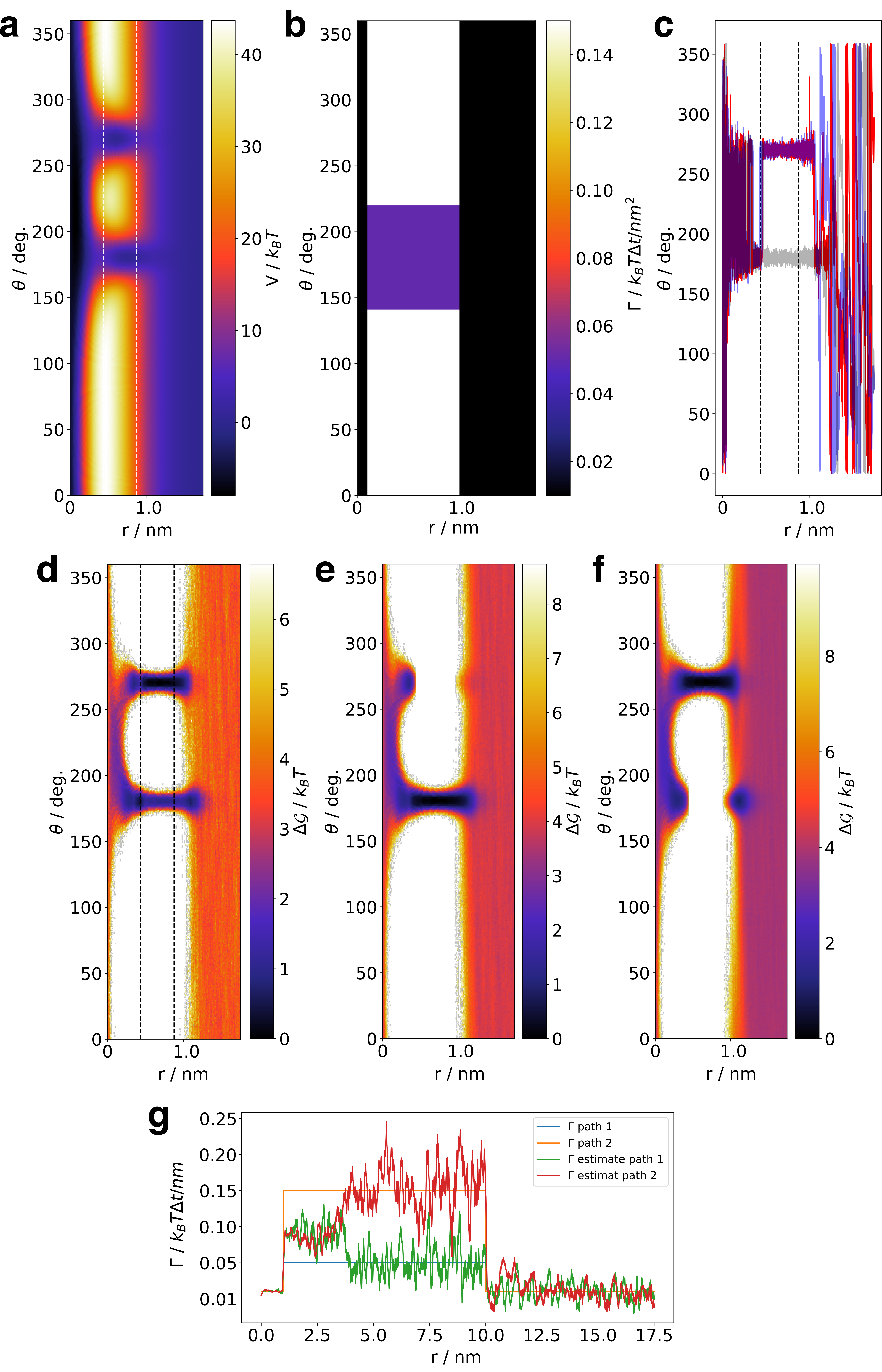
Figure S1: 2D model of ligand-protein dissociation. (a) Potential energy landscape $V(r,\theta)$ including borders for path discrimination at $r\in[0.44,0.875]$ nm. (b) Friction field ${\it{\Gamma}}(r,\theta)$. (c) Representative examples of crossing trajectories, exhibiting jumps at the beginning of the path separation domain. (d) Sampling of the density obtained from 5000 trajectories for the full system, and for (e) path 1 and (f) path 2. (g) Friction estimate ${\it{\Gamma}}$ from targeted MD simulations, smoothed by a window average filter with 0.0125 nm width. Before path separation, ${\it{\Gamma}}$ is estimated as a mean of the two true path friction coefficients. After path separation, estimates of ${\it{\Gamma}}$ fluctuate around the correct value.

S1.2 Rate estimation

To compare the kinetics of the 2D model defined by the potential $V(r_{1},r_{2})$ [Eq. (47)], and the path-separated 1D models using the respective pathway free energies $\Delta\mathcal{G}_{k}(r)$, we performed standard Langevin simulations governed by

$$\text{2D:}\quad m\ddot{{\boldsymbol{r}}} =-\frac{\partial V}{\partial{\boldsymbol{r}}}-{\it{\Gamma}}\dot{{\boldsymbol{r}}}+{\boldsymbol{\eta}}\;,$$ (49)

$$\text{path 1:}\quad m\ddot{r} =-\frac{\partial\mathcal{G}_{1}}{\partial r}-{\it{\Gamma}}r+\eta\;,\quad\quad\text{path 2:}\quad m\ddot{r}=-\frac{\partial\mathcal{G}_{2}}{\partial r}-{\it{\Gamma}}r+\eta\;,$$ (50)

where $\eta=\sqrt{2\mathrm{k}_{\mathrm{B}}T\,{\it{\Gamma}}}\mathcal{R}$. We used a mass $m=0.8$ kg/mol, constant friction ${\it{\Gamma}}_{k}=$ 20 kg/(mol ps) and temperature $T=300$ K.

In the 2D case, we used a simple Euler integration scheme to propagate $10\times 1\,\mu$s-long trajectories, where 42 start in the associated and 8 in the dissociated state, employing an integration time-step of 1 fs. We saved the positions $(r_{1},r_{2})$ for every ns. At $r=1.75$ nm, we introduced a reflective wall by a flip of the position and velocity components perpendicular to the wall. We calculated the waiting times of the associated and dissociated state, by tracking the number of frames in a state until leaving, using geometrical cores at $r=0.2$ nm and 1.4 nm, respectively. The rates $k_{\text{off}}$ and $k_{\text{on}}$ are then estimated by the inverse of the average waiting time, for each trajectory individually. We report their average and standard deviation in Table I of the main text.

We also performed biased simulations of the 2D system by constraining the distance to the center as $r=r_{0}+vt$, where we use $r_{0}=0.01$ nm and $v=0.01$ m/s. In particular, we integrate the constrained Langevin dynamics by transforming the equations of motion to polar coordinates, calculating the forces acting on $r$ and $\theta$ as usual, but then updating $r$ to conform to its constraint and recording the forces on $r$ as the constraint force. We finally compute the work by integrating these forces. Sampling from an initial unbiased distribution in $\theta$ and $\dot{\theta}$ at fixed $r_{0}$, we pull 10000 trajectories towards $r=1.75$ nm. By separating the trajectories using pathway 1 and 2, respectively, we use Jarzynski’s equality to calculate the pathway free energy.

Using these estimates of the pathway free energy, we performed one-dimensional Langevin simulations using the mass and friction given above. We simulated $10\times 1$ ms long simulations for both pathway 1 (45 starting in the associated, 5 in the dissociated state) and pathway 2 (40, 10), again with $\delta t=1$ fs and a reflective wall at $1.75$ nm. We computed the rates and weigh them by the probabilities obtained by Eq. (26) of the main text, reported in Table I of the main text.

Appendix S2 Normality test of the work distribution $P(W)$

In addition to estimating the probability distribution $P(W)$ via a histogram of the sampled work $W$ at a specific value of coordinate $x$, we can evaluate the normal probability plot of that sample. To this end, we employ the scipy.stats function probplot, which compares the points of the computed work to the quantiles of the corresponding normal distribution (the probit), such that the deviations reveal a non-Gaussian shape. In particular, we sort the work sample in increasing order and plot them against equidistant points of the inverse of the cumulative distribution function. Deviations from a straight line reveal an underlying non-Gaussian distribution.

Appendix S3 Trypsin-benzamidine complex:
PCA on ligand-protein contacts

Supporting References

References

- (1) C. Chipot and A. Pohorille, Free Energy Calculations, Springer, Berlin, 2007.
- (2) D. J. Wales, Energy Landscapes, Cambridge University Press, Cambridge, 2003.
- (3) P. Faccioli, M. Sega, F. Pederiva, and H. Orland, Dominant pathways in protein folding, Phys. Rev. Lett. 97, 108101 (2006).
- (4) C. Dellago and P. Bolhuis, Transition path sampling and other advanced simulation techniques for rare events, Adv. Polymer Sci. 221 (2016).
- (5) D. M. Zuckerman and L. T. Chong, Weighted ensemble simulation: Review of methodology, applications, and software, Annu. Rev. Biophys. 46, 43 (2017).
- (6) R. Capelli, P. Carloni, and M. Parrinello, Exhaustive Search of Ligand Binding Pathways via Volume-Based Metadynamics, J. Phys. Chem. Lett. , 3495 (2019).
- (7) R. Capelli, A. Bochicchio, G. Piccini, R. Casasnovas, P. Carloni, and M. Parrinello, Chasing the Full Free Energy Landscape of Neuroreceptor/Ligand Unbinding by Metadynamics Simulations., J. Chem. Theory Comput. 15, 3354 (2019).
- (8) J. Rydzewski and O. Valsson, Finding multiple reaction pathways of ligand unbinding, J. Chem. Phys. 150, 221101 (2019).
- (9) M. Bianciotto, P. Gkeka, D. B. Kokh, R. C. Wade, and H. Minoux, Contact Map Fingerprints of Protein-Ligand Unbinding Trajectories Reveal Mechanisms Determining Residence Times Computed from Scaled Molecular Dynamics., J. Chem. Theory Comput. 17, 6522 (2021).
- (10) A. Nunes-Alves, D. B. Kokh, and R. C. Wade, Ligand unbinding mechanisms and kinetics for T4 lysozyme mutants from RAMD simulations, Curr. Res. Struct. Biol. 3, 106 (2021).
- (11) J. Hénin, T. Lelièvre, M. R. Shirts, O. Valsson, and L. Delemotte, Enhanced sampling methods for molecular dynamics simulations, LiveCoMS 4, 1583 (2022).
- (12) S. Wolf and G. Stock, Targeted molecular dynamics calculations of free energy profiles using a nonequilibrium friction correction, J. Chem. Theory Comput. 14, 6175 (2018).
- (13) S. Wolf, B. Lickert, S. Bray, and G. Stock, Multisecond ligand dissociation dynamics from atomistic simulations, Nat. Commun. 11, 2918 (2020).
- (14) M. Post, S. Wolf, and G. Stock, Molecular origin of driving-dependent friction in fluids, J. Chem. Theory Comput. 18, 2816 – 2825 (2022).
- (15) P. Tiwary, V. Limongelli, M. Salvalaglio, and M. Parrinello, Kinetics of protein–ligand unbinding: Predicting pathways, rates, and rate-limiting steps, Proc. Natl. Acad. Sci. USA 112, E386 (2015).
- (16) N. Plattner and F. Noé, Protein conformational plasticity and complex ligand-binding kinetics explored by atomistic simulations and Markov models, Nat. Commun. 6, 7653 (2015).
- (17) I. Teo, C. G. Mayne, K. Schulten, and T. Lelievre, Adaptive Multilevel Splitting Method for Molecular Dynamics Calculation of Benzamidine-Trypsin Dissociation Time, J. Chem. Theory Comput. 12, 2983 (2016).
- (18) C. Jarzynski, Nonequilibrium equality for free energy differences, Phys. Rev. Lett. 78, 2690 (1997).
- (19) D. A. Hendrix and C. Jarzynski, A “fast growth” method of computing free energy differences, J. Chem. Phys. 114, 5974 (2001).
- (20) C. Dellago and G. Hummer, Computing equilibrium free energies using non-equilibrium molecular dynamics, Entropy 16, 41 (2014).
- (21) F. M. Ytreberg and D. M. Zuckerman, Efficient use of nonequilibrium measurement to estimate free energy differences for molecular systems, J. Comput. Chem. 25, 1749 (2004).
- (22) I. Echeverria and L. M. Amzel, Estimation of Free-Energy Differences from Computed Work Distributions: An Application of Jarzynski’s Equality, J. Phys. Chem. B 116, 10986 (2012).
- (23) P. Billingsley, Probability and Measure, Wiley, 1995.
- (24) M. Jäger, T. Koslowski, and S. Wolf, Predicting Ion Channel Conductance via Dissipation-Corrected Targeted Molecular Dynamics and Langevin Equation Simulations, J. Chem. Theory Comput. 18, 494 (2022).
- (25) S. Doudou, N. A. Burton, and R. H. Henchman, Standard Free Energy of Binding from a One-Dimensional Potential of Mean Force, J. Chem. Theory Comput. 5, 909 (2009).
- (26) M. Post, S. Wolf, and G. Stock, Principal component analysis of nonequilibrium molecular dynamics simulations, J. Chem. Phys. 150, 204110 (2019).
- (27) F. Guillain and D. Thusius, Use of proflavine as an indicator in temperature-jump studies of the binding of a competitive inhibitor to trypsin, J. Am. Chem. Soc. 92, 5534 (1970).
- (28) M. Marquart, J. Walter, J. Deisenhofer, W. Bode, and R. Huber, The geometry of the reactive site and of the peptide groups in trypsin, trypsinogen and its complexes with inhibitors, Acta Crystallogr. B 39, 480 (1983).
- (29) I. Buch, T. Giorgino, and G. De Fabritiis, Complete reconstruction of an enzyme-inhibitor binding process by molecular dynamics simulations, Proc. Natl. Acad. Sci. USA 108, 10184 (2011).
- (30) L. W. Votapka, B. R. Jagger, A. Heyneman, and R. E. Amaro, SEEKR: simulation enabled estimation of kinetic rates, a computational tool to estimate molecular kinetics and its application to trypsin–benzamidine binding, J. Phys. Chem. B 121, 3597 (2017).
- (31) R. M. Betz and R. O. Dror, How Effectively Can Adaptive Sampling Methods Capture Spontaneous Ligand Binding?, J. Chem. Theory Comput. 15, 2053 (2019).
- (32) J. Schlitter, M. Engels, and P. Krüger, Targeted molecular dynamics - a new approach for searching pathways of conformational transitions, J. Mol. Graph. 12, 84 (1994).
- (33) C. R. Harris et al., Array programming with NumPy, Nature 585, 357 (2020).
- (34) P. Virtanen et al., SciPy 1.0: fundamental algorithms for scientific computing in Python, Nat. Methods 17, 261 (2020).
- (35) W. McKinney, Data structures for statistical computing in python., in Proceedings of the 9th Python in Science Conference., edited by S. van der Walt and J. Millman, pages 51–56, 2010.
- (36) J. D. Hunter, Matplotlib: A 2D graphics environment, Comput. Sci. Eng. 9, 90 (2007).
- (37) J. Racine, gnuplot 4.0: a portable interactive plotting utility, J. Appl. Econ. 21, 133 (2006).
- (38) T. Kluyver et al., Jupyter Notebooks-a publishing format for reproducible computational workflows., in Positioning and Power in Academic Publishing, edited by F. Loizides and B. Schmidt, pages 87–90, IOP Press, 2016.
- (39) R. Zwanzig, Nonlinear generalized Langevin equations, J. Stat. Phys. 9, 215 (1973).
- (40) M. R. Sørensen and A. F. Voter, Temperature-accelerated dynamics for simulation of infrequent events, J. Chem. Phys. 112, 9599 (2000).
- (41) A. R. Henderson, Testing experimental data for univariate normality., Clin. Chim. Acta 366, 112 (2006).
- (42) S. R. Logan and D. Wilmer, Fundamentals of chemical kinetics, volume 10, Longman London, 1996.
- (43) F. Noé and C. Clementi, Collective variables for the study of long-time kinetics from molecular trajectories: theory and methods, Curr. Opin. Struct. Biol. 43, 141 (2017).
- (44) F. Sittel and G. Stock, Perspective: Identification of collective coordinates and metastable states of protein dynamics, J. Chem. Phys. 149, 150901 (2018).
- (45) M. Ernst, F. Sittel, and G. Stock, Contact- and distance-based principal component analysis of protein dynamics, J. Chem. Phys. 143, 244114 (2015).
- (46) A. Amadei, A. B. M. Linssen, and H. J. C. Berendsen, Essential dynamics of proteins, Proteins 17, 412 (1993).
- (47) A. Altis, M. Otten, P. H. Nguyen, R. Hegger, and G. Stock, Construction of the free energy landscape of biomolecules via dihedral angle principal component analysis, J. Chem. Phys. 128, 245102 (2008).
- (48) G. Hummer, A. E. Garcia, and S. Garde, Helix nucleation kinetics from molecular simulations in explicit water, Proteins 42, 77 (2001).
- (49) M. A. Rohrdanz, W. Zheng, and C. Clementi, Discovering mountain passes via torchlight: Methods for the definition of reaction coordinates and pathways in complex macromolecular reactions, Annu. Rev. Phys. Chem. 64, 295 (2013).
- (50) A. Glielmo, B. E. Husic, A. Rodriguez, C. Clementi, F. Noé, and A. Laio, Unsupervised learning methods for molecular simulation data, Chem. Rev. 121, 9722 (2021).
- (51) M. Amaral, D. B. Kokh, J. Bomke, A. Wegener, H. P. Buchstaller, H. M. Eggenweiler, P. Matias, C. Sirrenberg, R. C. Wade, and M. Frech, Protein conformational flexibility modulates kinetics and thermodynamics of drug binding., Nat. Commun. 8, 2276 (2017).
- (52) S. Bray, V. Tänzel, and S. Wolf, Ligand Unbinding Pathway and Mechanism Analysis Assisted by Machine Learning and Graph Methods, J. Chem. Inf. Model. 62, 4591 (2022).
- (53) J. Servantie and P. Gaspard, Methods of calculation of a friction coefficient: application to nanotubes, Phys. Rev. Lett. 91, 185503 (2003).
- (54) As practical guideline, we recommend to first perform a set of 100 simulations for a pulling velocity of m/s and check if a path separation with contact distances is possible. If this does not lead to a successful removal of the friction overestimation artifact (see Fig. 1c), a similar study should be done for m/s. If the simulations then become dominated by crossing trajectories (see Ref.Wolf20 , Fig. S4c), the system may be not suited for a dcTMD analysis. We note that in all our investigations carried out so far, Wolf18 ; Wolf20 ; Post22 ; Jager22 ; Bray22 the systems were treatable with dcTMD, but the major challenge was finding a suitable orthogonal coordinate .
- (55) M. J. Abraham, T. Murtola, R. Schulz, S. Pall, J. C. Smith, B. Hess, and E. Lindahl, Gromacs: High performance molecular simulations through multi-level parallelism from laptops to supercomputers, SoftwareX 1, 19 (2015).
- (56) V. Hornak, R. Abel, A. Okur, B. Strockbine, A. Roitberg, and C. Simmerling, Comparison of multiple Amber force fields and development of improved protein backbone parameters, Proteins 65, 712 (2006).
- (57) R. B. Best and G. Hummer, Optimized molecular dynamics force fields applied to the helix-coil transition of polypeptides, J. Phys. Chem. B 113, 9004 (2009).
- (58) J. Wang and R. Brüschweiler, 2D entropy of discrete molecular ensembles, J. Chem. Theory Comput. 2, 18 (2006).
- (59) J. M. Wang, R. M. Wolf, J. W. Caldwell, P. A. Kollman, and D. A. Case, Development and testing of a general amber force field, J. Comput. Chem. 25, 1157 (2004).
- (60) F. Neese, The ORCA program system, WIREs Comput. Mol. Sci. 2, 73 (2012).
- (61) T. Lu and F. Chen, Multiwfn: A multifunctional wavefunction analyzer, J. Comput. Chem. 33, 580 (2012).
- (62) W. L. Jorgensen, J. Chandrasekhar, J. D. Madura, R. W. Impey, and M. Klein, Comparison of simple potential functions for simulating liquid water, J. Chem. Phys. 79, 926 (1983).
- (63) F. Sittel, T. Filk, and G. Stock, Principal component analysis on a torus: Theory and application to protein dynamics, J. Chem. Phys. 147, 244101 (2017).
- (64) H. Wu, F. Paul, C. Wehmeyer, and F. Noé, Multiensemble Markov models of molecular thermodynamics and kinetics, Proc. Natl. Acad. Sci. USA 113, E3221 (2016).
- (65) H. Fu, Y. Zhou, X. Jing, X. Shao, and W. Cai, Meta-Analysis Reveals That Absolute Binding Free-Energy Calculations Approach Chemical Accuracy, J. Med. Chem. 65, 12970 (2022).
- (66) J. M. L. Ribeiro, P. Bravo, Y. Wang, and P. Tiwary, Reweighted autoencoded variational bayes for enhanced sampling (rave), J. Chem. Phys. 149, 072301 (2018).
- (67) J. M. L. Ribeiro, D. Provasi, and M. Filizola, A combination of machine learning and infrequent metadynamics to efficiently predict kinetic rates, transition states, and molecular determinants of drug dissociation from G protein-coupled receptors, J. Chem. Phys. 153, 124105 (2020).
- (68) M. Bertazzo, D. Gobbo, S. Decherchi, and A. Cavalli, Machine Learning and Enhanced Sampling Simulations for Computing the Potential of Mean Force and Standard Binding Free Energy., J. Chem. Theory Comput. 17, 5287 (2021).
- (69) M. Badaoui et al., Combined Free-Energy Calculation and Machine Learning Methods for Understanding Ligand Unbinding Kinetics., J. Chem. Theory Comput. 18, 2543 (2022).
- (70) G. Yuan, P. Sun, J. Zhao, and D. Li, A review of moving object trajectory clustering algorithms, Artif. Intel.l Rev. 47, 123 – 144 (2017).
- (71) G. Diez, D. Nagel, and G. Stock, Correlation-based feature selection to identify functional dynamics in proteins, J. Chem. Theory Comput. 18, 5079 – 5088 (2022).
- (72) G. R. Haynes, G. A. Voth, and E. Pollak, A theory for the activated barrier crossing rate constant in systems influenced by space and time dependent friction, J. Chem. Phys. 101, 7811 (1994).

References

- (1) M. Post, S. Wolf, and G. Stock, Principal component analysis of nonequilibrium molecular dynamics simulations, J. Chem. Phys. 150, 204110 (2019).