RIS-Aided Monostatic Sensing and Object Detection with Single and Double Bounce Multipath

Abstract

We propose a framework for monostatic sensing by a user equipment (UE), aided by a reconfigurable intelligent surface (RIS) in environments with single- and double-bounce signal propagation. We design appropriate UE-side precoding and combining, to facilitate signal separation. We derive the adaptive detection probabilities of the resolvable signals, based on the geometric channel parameters of the links. Then, we estimate the passive objects using both the double-bounce signals via passive RIS (i.e., RIS-sensing) and the single-bounce multipath direct to the objects (i.e., non-RIS-sensing), based on a mapping filter. Finally, we provide numerical results to demonstrate that effective sensing can be achieved through the proposed framework.

I Introduction

isac is expected to be a key functionality in sixth generation (6G) communications, enabling a variety of applications [1]. ris facilitate integrated sensing and communications (ISAC) thanks to the enhanced coverage, obtained by reflecting the received signal power, or to the creation of a controllable wireless propagation environment by proper design of the phase profiles [2, 3], representing thus one of the 6G enablers [4].

Monostatic sensing with RIS is relatively under-explored. Relevant works in this direction include [5, 6, 7, 8, 9, 10, 11, 12]. The authors of [5] introduce case studies of reconfigurable intelligent surface (RIS)-enabled sensing and localization, including the double-bounce signal scenario, where the signal reflected by the RIS can impinge on a scattering point (SP) before being received back at the UE (denoted by UE-RIS-SP-UE). In [6], several RISs are regarded as controllable passive objects with a priori unknown location. Paths of the form UE-SP-UE and UE-RIS-UE are considered to map the environment and localize the UE. In [7], an RIS is used to overcome line-of-sight (LOS) blockage in radar sensing. Radar performance is further studied in [8, 9], focusing on a single-SP scenario, which simplifies the problem significantly. Studies focused on ISAC include [10, 11], where in [10] an RIS is used to reduce multi-user interference at the user equipments due to the joint radar and communication signal sent by a base station (BS), while [11] considers allocating separated RIS elements between sensing and communications. Finally [12] goes even further and considers a hybrid RIS that can actively sense the environment. Despite these studies on RIS-aided sensing, there are still several unsolved problems in the monostatic regime (see Fig. 1): how to separate the different single and double-bounce signals corresponding to the several SPs; how to design UE precoders and combiners to enable tractable processing; how to fuse information coming from single-bounce and double-bounce signals associated with a single SP; and how much RIS can help when a priori information about the SPs is unavailable.

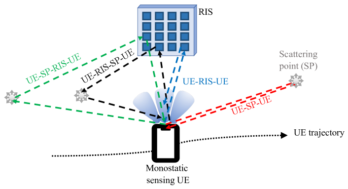
Figure 1: Illustration of the considered sensing scenario where a single monostatic UE maps the environment (described by scattering points) with the support of an RIS.

In this paper, we propose a framework of RIS-aided monostatic range-angle sensing to estimate the locations of several passive objects (i.e., SPs). The contributions are as follows: (i) we derive the signal model that encompasses all single- and double-bounce paths via the RIS; (ii) to enable separation of the different paths, we propose a suitably-designed UE-side precoding and combining scheme; (iii) we derive analytical expressions for the detection probabilities of the objects, based on the separated observations; (iv) finally, we fuse the different observations and map the SPs as the UE explores the environment. This fusion is based on two state-of-the-art Poisson multi-Bernoulli (PMB) filters [13, 14], one with the double-bounce signals via passive RIS; and the other with the single-bounce signals direct to SPs. Sensing results are finally merged into one map by the generalized covariance intersection (GCI) fusion method [15]. Numerical results reveal that, under the considered UE precoding and combining and random RIS configurations, the single-bounce path provides the most information about the SPs, followed by the path UE-RIS-SP-UE, while the path UE-SP-RIS-UE is less informative.

II System and Signal Models

In this section, we introduce proper models for monostatic sensing and object detection, aided by a single RIS.

II-A System Setup

Consider the generic scenario adapted from [9, Fig. 1 (b) and (d)] in Fig. 1, where a full-duplex UE transmits a signal using an antenna array and receives the backscattered signal from both passive objects (SPs) and an RIS. Under this scenario, there are at least four different types of paths: two single-bounce paths, which are the path via the RIS, namely the path, UE-RIS-UE (shown in blue), and the conventional radar paths, UE-SP-UE (shown in red). There are also two double-bounce paths per SP, namely the path, UE-RIS-SP-UE (shown in black), and the path, UE-SP-RIS-UE (shown in green). Higher-order bounces are ignored, as they are much weaker. Hence, each SP can be observed up to 3 times, depending on the corresponding end-to-end signal-to-noise ratio. Here, the signals for i) UE-RIS-UE, ii) UE-RIS-SP-UE, iii) UE-SP-RIS-UE can be controlled by the RIS while those in iv) UE-SP-UE cannot. The full-duplex UE and the RIS are equipped with uniform planar arrays, and their array sizes are respectively $N_{\mathrm{U}}=N_{\mathrm{U}}^{\mathrm{az}}\times N_{\mathrm{U}}^{\mathrm{el}}$ and $N_{\mathrm{R}}=N_{\mathrm{R}}^{\mathrm{az}}\times N_{\mathrm{R}}^{\mathrm{el}}$.

We denote the UE state at epoch $k$ by $\mathbf{s}_{k}=[\mathbf{x}_{\mathrm{U},k}^{\top},\alpha_{\mathrm{U},k},v_{\mathrm{U},k}]^{\top}$, where the elements are the location, heading, and speed, respectively. The RIS location is denoted by $\mathbf{x}_{\mathrm{R}}$, and the $l$-th SP location is denoted by $\mathbf{x}^{l}$. To handle the unknown number of SPs and their locations that specify the propagation environment, we model the SPs by a random finite set (RFS) $\mathcal{X}=\{\mathbf{x}^{1},\dots,\mathbf{x}^{n}\}$, with the set density $f(\mathcal{X})$ [16]. We assume the UE state (location, heading, and speed) and RIS location are known, to focus on the sensing performance.

II-B Signal and Channel Models

We adopt a deterministic channel model that considers only large-scale fading for all resolvable paths. The received orthogonal frequency-division multiplexing (OFDM) signal of the $s$-th subcarrier at the $t$-th transmission of time epoch $k$ is modeled as

$$\mathbf{y}_{k,t,s}\triangleq \bigg{(}\sum_{l=0}^{L}\underbrace{\alpha_{k,l}\nu_{t}(\bm{\phi}_{k,l})\mathbf{a}_{\mathrm{U}}(\bm{\theta}_{k,l})\mathbf{a}_{\mathrm{U}}^{\top}(\bm{\theta}_{k,0})d_{s}(\tau_{k,l})}_{\text{i) UE-RIS-UE}~{}(l=0),~{}\text{ii) UE-RIS-SPs-UE}~{}(l\neq 0)}$$ (1)

$$+\sum_{l=1}^{L}\underbrace{\alpha_{k,l}\nu_{t}(\bm{\phi}_{k,l})\mathbf{a}_{\mathrm{U}}(\bm{\theta}_{k,0})\mathbf{a}_{\mathrm{U}}^{\top}(\bm{\theta}_{k,l})d_{s}(\tau_{k,l})}_{{\text{iv) UE-SPs-RIS-UE~{}paths}}}$$

$$+\sum_{l=1}^{L}\underbrace{\beta_{k,l}\mathbf{a}_{\mathrm{U}}(\bm{\theta}_{k,l})\mathbf{a}_{\mathrm{U}}^{\top}(\bm{\theta}_{k,l})d_{s}(\bar{\tau}_{k,l})}_{\text{iii) UE-SPs-UE~{}paths}}\bigg{)}{\mathbf{f}}_{k,t}+\mathbf{n}_{k,t,s}.$$

The parameters $\alpha_{k,l}$ and $\beta_{k,l}$ are respectively the complex path gains of the controlled and uncontrolled signals; $\mathbf{a}_{\mathrm{R}}(\cdot)$ and $\mathbf{a}_{\mathrm{U}}(\cdot)$ are respectively the array vectors [17, eqs. (13)–(15)] of the RIS and UE with $\bm{\phi}_{k,l}=[\phi_{k,l}^{\mathrm{az}},\phi_{k,l}^{\mathrm{el}}]^{\top}$ denoting the azimuth and elevation of the angle-of-arrival (AoA) and angle-of-departure (AoD) at the RIS and $\bm{\theta}_{k,l}=[\theta_{k,l}^{\mathrm{az}},\theta_{k,l}^{\mathrm{el}}]^{\top}$ the AoA and AoD at the UE; $d_{s}(\tau)\triangleq e^{-j2\pi(s-1)\tau\Delta_{f}}$ is the phase shift linked to the time-of-arrival (ToA) with $\tau_{k,l}$ and $\bar{\tau}_{k,l}$ denoting the ToAs for the controlled and uncontrolled signals; $\Delta_{f}$ denotes the subcarrier spacing; ${\mathbf{f}}_{k,{t}}$ denotes the precoder with $\|{\mathbf{f}}_{k,{t}}\|^{2}=1$; and $\mathbf{n}_{k,t,s}\sim\mathcal{CN}(\bm{0}_{\mathrm{UE}_{N}},N_{0}\mathbf{I}_{N_{\mathrm{U}}})$ denotes the complex Gaussian noise. Finally, we denote the RIS phase profile $\bm{\Omega}_{\mathrm{R},k,t}\triangleq\mathrm{diag}(\bm{\omega}_{k,t})$, where $\bm{\omega}_{k,t}\triangleq[\omega_{k,t}^{1},\dots,\omega_{k,t}^{N_{\mathrm{R}}}]^{\top}$, so that $\nu_{t}(\bm{\phi}_{k,l})\triangleq\mathbf{a}_{\mathrm{R}}^{\top}(\bm{\phi}_{k,l})\bm{\Omega}_{\mathrm{R},k,t}\mathbf{a}_{\mathrm{R}}(\bm{\phi}_{k,0})$. The channel parameters are defined in Appendix A. In the following, we assume that $T/\Delta_{f}$ is sufficiently small so that Doppler effects can be considered negligible.

II-C Precoders and RIS Phase Profiles

The precoders and the RIS phase profiles follow a specific time sequence [18, 17] for orthogonal design (that indicates $\sum_{t}\bm{\omega}_{t,k}=0$): $\tilde{\bm{\omega}}_{\tilde{t},k}\in\mathbb{C}^{N_{\mathrm{R}}\times 1}$ for $\tilde{t}=1,\dots,T/2$, and $\bm{\omega}_{2\tilde{t}-1,k}\triangleq\tilde{\bm{\omega}}_{\tilde{t},k}$, $\bm{\omega}_{2\tilde{t},k}\triangleq-\tilde{\bm{\omega}}_{\tilde{t},k}$, and $\mathbf{f}_{2\tilde{t}-1,k}\triangleq\mathbf{f}_{2\tilde{t},k}\triangleq\tilde{\mathbf{f}}_{\tilde{t},k}$. The $n$-th element of RIS phase profile is denoted by $[\tilde{w}_{\tilde{t},k}]^{n}=e^{j\phi_{\tilde{t},k}^{n}}$, where $\phi_{\tilde{t},k}^{n}$ is the RIS phase.

III Signal Separation

In this section, we propose an approach for separating the different contributions in the received signal (1).

III-A RIS and Non-RIS Signals

By leveraging the orthogonal RIS phase design, we divide the received signals into the controlled (i–iii) and uncontrolled (iv) signals as follows, for $\tilde{t}=1,\dots,T/2$

$$\tilde{\mathbf{y}}_{k,\tilde{t},s}^{\mathrm{R}}\triangleq\,\frac{1}{2}(\mathbf{y}_{k,2t,s}-\mathbf{y}_{k,2t-1,s})$$ (2)

$$=\,\sum_{l=0}^{L}\alpha_{k,l}\nu_{\tilde{t}}(\bm{\phi}_{k,l})\mathbf{a}_{\mathrm{U}}(\bm{\theta}_{k,l})\mathbf{a}_{\mathrm{U}}^{\top}(\bm{\theta}_{k,0})d_{s}(\tau_{k,l})\tilde{\mathbf{f}}_{k,\tilde{t}}$$ (3)

$$+\sum_{l=1}^{L}\alpha_{k,l}\nu_{\tilde{t}}(\bm{\phi}_{k,l})\mathbf{a}_{\mathrm{U}}(\bm{\theta}_{k,0})\mathbf{a}_{\mathrm{U}}^{\top}(\bm{\theta}_{k,l})d_{s}(\tau_{k,l})\tilde{\mathbf{f}}_{k,\tilde{t}}+\tilde{\mathbf{n}}_{k,\tilde{t},s}^{\mathrm{R}},$$

and

$$\tilde{\mathbf{y}}_{k,\tilde{t},s}^{\mathrm{N}}\triangleq \,\frac{1}{2}(\mathbf{y}_{k,2t,s}+\mathbf{y}_{k,2t-1,s})$$ (4)

$$= \,\sum_{l=1}^{L}\beta_{k,l}\mathbf{a}_{\mathrm{U}}(\bm{\theta}_{k,l})\mathbf{a}_{\mathrm{U}}^{\top}(\bm{\theta}_{k,l})d_{s}(\bar{\tau}_{k,l})\tilde{\mathbf{f}}_{k,\tilde{t}}+\tilde{\mathbf{n}}_{k,\tilde{t},s}^{\mathrm{N}},$$ (5)

where $\tilde{\mathbf{n}}_{k,\tilde{t},s}^{\mathrm{R}}$ and $\tilde{\mathbf{n}}_{k,\tilde{t},s}^{\mathrm{N}}$ are independent complex Gaussian noise contributions, distributed as $\mathcal{CN}(\bm{0}_{N_{\mathrm{U}}},N_{0}\mathbf{I}_{N_{\mathrm{U}}}/2)$. We assume that the RIS signal is always visible, and $\bm{\phi}_{k,0}$ and $\bm{\theta}_{k,0}$ are known, due to the knowledge of the UE state.

III-B Separation of the RIS Signals

In (3), the path to and from the RIS appear together, so that without suitable processing, up to $2L+1$ path will be present. To avoid this, we propose a method to separate the UE-SP-RIS-UE paths (second term in (3)) from the UE-RIS-SP-UE paths (first term in (3)), by designing the precoder and combiner at the UE, inspired by the approach from [19]. In particular, we divide up the $T/2$ available transmissions into $T_{1}$ transmissions towards the RIS, with $\tilde{\mathbf{f}}_{k,\tilde{t}}=\mathbf{a}^{*}_{\mathrm{U}}(\bm{\theta}_{k,0})/\|\mathbf{a}_{\mathrm{U}}(\bm{\theta})\|$ and $T_{2}=T/2-T_{1}$ transmissions with a null towards the RIS, i.e., with $\tilde{\mathbf{f}}_{k,\tilde{t}}^{\mathrm{H}}\mathbf{a}_{\mathrm{U}}(\bm{\theta}_{k,0})=0$. For each transmission, we use the (invertible and thus lossless) combiner $\mathbf{W}_{k}=[\mathbf{a}_{\mathrm{U}}(\bm{\theta}_{k,0})/\|\mathbf{a}_{\mathrm{U}}(\bm{\theta})\|,\mathbf{W}_{k,\perp}]$ such that $\mathbf{W}_{k}^{\mathrm{H}}\mathbf{W}_{k}=\mathbf{I}_{N_{\mathrm{U}}}$ and $\mathbf{W}_{k,\perp}^{\mathrm{H}}\mathbf{a}_{\mathrm{U}}(\bm{\theta}_{k,0})=\bm{0}_{N_{\mathrm{U}}-1}$.

III-B1 Observation during $T_{1}$TEXT Transmissions toward RIS

During the transmissions when $\tilde{\mathbf{f}}_{k,\tilde{t}}=\mathbf{a}^{*}_{\mathrm{U}}(\bm{\theta}_{k,0})/\|\mathbf{a}_{\mathrm{U}}(\bm{\theta}\|$, the output of the combiner will be $\mathbf{W}^{\mathrm{H}}_{k}\tilde{\mathbf{y}}_{k,\tilde{t},s}^{\mathrm{R}}$. To remove the unwanted UE-RIS-UE path, we discard the first entry and denote the remainder by $\mathbf{\bar{y}}_{k,\tilde{t},s}^{\mathrm{D}}\in\mathbb{C}^{N_{\mathrm{U}}\times 1}$ (‘D’ is used for directional), which is expressed as

$$\mathbf{\bar{y}}_{k,\tilde{t},s}^{\mathrm{D}} =\mathbf{W}^{\mathrm{H}}_{k,\perp}\tilde{\mathbf{y}}_{k,\tilde{t},s}^{\mathrm{R}}=\mathbf{W}^{\mathrm{H}}_{k,\perp}\tilde{\mathbf{n}}_{k,\tilde{t},s}^{\mathrm{R}}$$ (6)

$$+\sqrt{N_{\mathrm{U}}}\sum_{l=0}^{L}\alpha_{k,l}\nu_{\tilde{t}}(\bm{\phi}_{k,l})\mathbf{W}^{\mathrm{H}}_{k,\perp}\mathbf{a}_{\mathrm{U}}(\bm{\theta}_{k,l})d_{s}(\tau_{k,l})$$

since $\mathbf{a}_{\mathrm{U}}^{\top}(\bm{\theta}_{k,0})\tilde{\mathbf{f}}_{k,\tilde{t}}=\|\mathbf{a}_{\mathrm{U}}(\bm{\theta}_{k,0})\|=\sqrt{N_{\mathrm{U}}}$.

III-B2 Observation during $T_{2}$TEXT Transmissions with null to RIS

During the remaining $T_{2}$ transmissions, the (arbitrary) precoders with null towards the RIS ensures that the first term in (3) is cancelled. In the observation after combining $\mathbf{W}^{\mathrm{H}}_{k}\tilde{\mathbf{y}}_{k,\tilde{t},s}^{\mathrm{R}}$, only the first entry contains information, since the remaining part $\mathbf{W}^{\mathrm{H}}_{k,\perp}\tilde{\mathbf{y}}_{k,\tilde{t},s}^{\mathrm{R}}$ only contains noise. Hence, the useful observation is $\bar{{y}}_{k,\tilde{t},s}^{\mathrm{O}}\in\mathbb{C}$ (‘O’ is used for orthogonal), with

$$\bar{{y}}_{k,\tilde{t},s}^{\mathrm{O}} =\frac{\mathbf{a}_{\mathrm{U}}^{\mathrm{H}}(\bm{\theta}_{k,0})}{\|\mathbf{a}_{\mathrm{U}}\|}\tilde{\mathbf{y}}_{k,\tilde{t},s}^{\mathrm{R}}=\frac{\mathbf{a}_{\mathrm{U}}^{\mathrm{H}}(\bm{\theta}_{k,0})}{\|\mathbf{a}_{\mathrm{U}}\|}\tilde{\mathbf{n}}_{k,\tilde{t},s}^{\mathrm{R}}$$ (7)

$$+\sqrt{N_{\mathrm{U}}}\sum_{l=1}^{L}\alpha_{k,l}\nu_{\tilde{t}}(\bm{\phi}_{k,l})\mathbf{a}_{\mathrm{U}}^{\top}(\bm{\theta}_{k,l})d_{s}(\tau_{k,l})\tilde{\mathbf{f}}_{k,\tilde{t}}.$$

In summary, we obtain the three types of refined signals corresponding to ii)–iv): ii) UE-RIS-SPs-UE to $\bar{\mathbf{y}}_{k,\tilde{t},s}^{\mathrm{D}}$ of (6), during $T_{1}$ transmissions ($\tilde{t}=1,\dots,T_{1}$); iii) UE-SPs-RIS-UE to ${{y}}_{t,\bar{t},s}^{\mathrm{O}}$ of (7), during $T_{2}=T/2-T_{1}$ transmissions ($\tilde{t}=T_{1}+1,\dots,T/2$); and iv) UE-SPs-UE to $\tilde{\mathbf{y}}_{k,\tilde{t},s}^{\mathrm{N}}$ of (5), during $T/2$ transmissions ($\tilde{t}=1,\dots,T/2$).

IV Detection Probability

We compute the DPs, $p_{\mathrm{U}}^{\mathrm{D}}(\mathbf{x}^{l},\mathbf{s}_{k})$, $p_{\mathrm{U}}^{\mathrm{O}}(\mathbf{x}^{l},\mathbf{s}_{k})$, and $p_{\mathrm{U}}^{\mathrm{N}}(\mathbf{x}^{l},\mathbf{s}_{k})$, for all paths. Following [20], we will focus on a single path at each signal and omit the time index $k$ for notational simplicity.

IV-A Hypothetical Observation

Paths in the separated signals ii)–iv) are expressed as

$$\mathbf{\bar{y}}_{l,\tilde{t},s}^{\mathrm{D}}\triangleq \,\alpha_{l}\sqrt{N_{\mathrm{U}}}\nu_{\tilde{t}}(\bm{\phi}_{l})\mathbf{W}_{\perp}^{\mathrm{H}}\mathbf{a}_{\mathrm{U}}(\bm{\theta}_{l})d_{s}(\tau_{l})+\mathbf{\bar{n}}_{l,\tilde{t},s}^{\mathrm{D}},$$ (8)

$$\bar{{y}}_{l,\tilde{t},s}^{\mathrm{O}}\triangleq \,\alpha_{l}\sqrt{N_{\mathrm{U}}}\nu_{\tilde{t}}(\bm{\phi}_{l})\mathbf{a}_{\mathrm{U}}^{\top}(\bm{\theta}_{l})\tilde{\mathbf{f}}_{\tilde{t}}d_{s}(\tau_{l})+\bar{{n}}_{l,\tilde{t},s}^{\mathrm{O}},$$ (9)

$$\tilde{\mathbf{y}}_{l,\tilde{t},s}^{\mathrm{N}}\triangleq \,\beta_{l}\mathbf{a}_{\mathrm{U}}(\bm{\theta}_{l})\mathbf{a}_{\mathrm{U}}^{\top}(\bm{\theta}_{l})\tilde{\mathbf{f}}_{\tilde{t}}d_{s}(\bar{\tau}_{l})+\tilde{\mathbf{n}}_{\tilde{t},s}^{\mathrm{N}}.$$ (10)

where $\mathbf{\bar{n}}_{l,\tilde{t},s}^{\mathrm{D}}=\mathbf{W}_{\perp}^{\mathrm{H}}\tilde{\mathbf{n}}_{\tilde{t},s}$ with $\mathbb{E}\{\mathbf{\bar{n}}_{l,\tilde{t},s}^{\mathrm{D}}(\mathbf{\bar{n}}_{l,\tilde{t},s}^{\mathrm{D}})^{\mathrm{H}}\}=N_{0}\mathbf{I}_{N_{\mathrm{U}}-1}$, $\bar{{n}}_{l,\tilde{t},s}^{\mathrm{O}}=\frac{\mathbf{a}_{\mathrm{U}}^{\mathrm{H}}(\bm{\theta}_{0})}{\|\mathbf{a}_{\mathrm{U}}\|}\tilde{\mathbf{n}}_{\tilde{t},s}$ with $\mathbb{E}\{\bar{{n}}_{l,\tilde{t},s}^{\mathrm{O}}(\bar{{n}}_{l,\tilde{t},s}^{\mathrm{O}})^{\mathrm{H}}\}=N_{0}$. We derive the detection probability related to $\mathbf{\bar{y}}_{l,\tilde{t},s}^{\mathrm{D}}$, while the other observations can be treated similarly. Let us define

$$\mathbf{p}_{l,\tilde{t},s}^{\mathrm{D}}\triangleq \sqrt{N_{\mathrm{U}}}\nu_{\tilde{t}}(\bm{\phi}_{l})\mathbf{W}_{\perp}^{\mathrm{H}}\mathbf{a}_{\mathrm{U}}(\bm{\theta}_{l})d_{s}(\tau_{l})$$ (11)

and then introduce compressed observations for the signals ii)–iv), computed by coherent combining over subcarriers and transmissions $\tilde{t}=1,\dots,T_{1}$ for ii), $\tilde{t}=T_{1}+1,\dots,T/2$ for iii), and $\tilde{t}=1,\dots,T/2$ for iv) as follows: $\rho_{l}^{\mathrm{D}}\triangleq\sum_{\tilde{t},s}(\mathbf{p}_{l,\tilde{t},s}^{\mathrm{D}})^{\mathrm{H}}\bar{\mathbf{y}}_{l,\tilde{t},s}^{\mathrm{D}}$ (and similarly $\rho_{l}^{\mathrm{O}}\triangleq\sum_{\tilde{t},s}({p}_{l,\tilde{t},s}^{\mathrm{O}})^{\mathrm{H}}\bar{{y}}_{l,\tilde{t},s}^{\mathrm{O}}$, and $\rho_{l}^{\mathrm{N}}\triangleq\sum_{\tilde{t},s}(\mathbf{p}_{l,\tilde{t},s}^{\mathrm{N}})^{\mathrm{H}}\tilde{\mathbf{y}}_{l,\tilde{t},s}^{\mathrm{N}}$). The observations are represented as $\rho_{l}^{\mathrm{D}}=\sum_{\tilde{t},s}\alpha_{l}\lVert\mathbf{p}_{l,\tilde{t},s}^{\mathrm{D}}\rVert^{2}+w_{l}^{\mathrm{D}},$ where the noise terms are defined as $w_{l}^{\mathrm{D}}\triangleq\sum_{\tilde{t},s}(\mathbf{p}_{l,\tilde{t},s}^{\mathrm{D}})^{\mathrm{H}}\mathbf{\bar{n}}_{l,\tilde{t},s}^{\mathrm{D}}$. We obtain new observations as follows: $\breve{y}_{l}^{\mathrm{D}}\triangleq\rho_{l}^{\mathrm{D}}/\sqrt{\mathbb{E}[\lvert w_{l}^{\mathrm{D}}\rvert^{2}]/2}$, where the expectation is computed as $\mathbb{E}[\lvert w_{l}^{\mathrm{D}}\rvert^{2}]=\tilde{P}_{l}^{\mathrm{D}}N_{0}/2$, in which $\tilde{P}_{l}^{\mathrm{D}}\triangleq\sum_{\tilde{t},s}\lVert\mathbf{p}_{l,\tilde{t},s}^{\mathrm{D}}\rVert^{2}$.

IV-B Detection Probabilities with Hypothetical Statistics

Now, we consider hypothetical statistics for signals ii)–iv) denoted as $\lvert\breve{{y}}_{l}^{\mathrm{D}}\rvert^{2}$, $\lvert\breve{{y}}_{l}^{\mathrm{O}}\rvert^{2}$, and $\lvert\breve{{y}}_{l}^{\mathrm{N}}\rvert^{2}$, which follow non-central chi-squared distribution with non-centrality parameter $\lambda_{l}^{\mathrm{D}}=4\alpha_{l}^{2}\tilde{P}_{l}^{\mathrm{D}}/N_{0}$ (and similarly $\lambda_{l}^{\mathrm{O}}$ and $\lambda_{l}^{\mathrm{N}}$). Finally, the DP for the $l$-th path of UE-RIS-SP-UE signal is computed as [9, eq.(13)]

$$p_{\mathrm{U}}^{\mathrm{D}}(\mathbf{x}^{l},\mathbf{s}) =f(\lvert\breve{y}_{l}^{\mathrm{D}}\rvert^{2}>\gamma)=Q_{1}\Big{(}\sqrt{\lambda_{l}^{\mathrm{D}}},\sqrt{\gamma}\Big{)},$$ (12)

where $Q_{1}(\cdot,\cdot)$ denotes the Marcum Q-function, and $\gamma=-2\log p_{\mathrm{FA}}$, in which $p_{\mathrm{FA}}$ is the false alarm probability. Similarly, $p_{\mathrm{U}}^{\mathrm{O}}(\mathbf{x}^{l},\mathbf{s})$ and $p_{\mathrm{U}}^{\mathrm{N}}(\mathbf{x}^{l},\mathbf{s})$ can be computed.

V Poisson Multi-Bernoulli Filtering for Passive Object Sensing

We first describe the measurements from the separated signals. Since each SP can give rise to up to 3 paths and thus 3 measurements, two problems occur: a data association problem concerning which UE-SP-UE, UE-RIS-SP-UE, and UE-SP-RIS-UE paths are related to the same SP, and a fusion problem regarding how to combine the associated measurements. To address these problems, we associate and fuse all the double-bounce measurements using ellipsoidal gating. Then, using the measurements, we run two independent PMB filters: one with single- and the other with double-bounce measurements. Finally, we perform periodic fusion. When possible, we will omit the time index $k$.

V-A Measurements

By applying a channel estimation routine at each time $k$ on the signals $\bar{\mathbf{y}}_{k,\tilde{t},s}^{\mathrm{D}}$, $\bar{{y}}_{k,\tilde{t},s}^{\mathrm{O}}$, and $\tilde{\mathbf{y}}_{k,\tilde{t},s}^{\mathrm{N}}$, we respectively obtain channel parameter sets $\mathcal{Z}_{k}^{\mathrm{D}}\triangleq\{\mathbf{z}_{k,1}^{\mathrm{D}},\dots,\mathbf{z}_{k,J_{k}^{\mathrm{D}}}^{\mathrm{D}}\}$, $\mathcal{Z}_{k}^{\mathrm{O}}\triangleq\{\mathbf{z}_{k,1}^{\mathrm{O}},\dots,\mathbf{z}_{k,J_{k}^{\mathrm{O}}}^{\mathrm{O}}\}$, and $\mathcal{Z}_{k}^{\mathrm{N}}\triangleq\{\mathbf{z}_{k,1}^{\mathrm{N}},\dots,\mathbf{z}_{k,J_{k}^{\mathrm{N}}}^{\mathrm{N}}\}$, where $J_{k}^{\mathrm{D}}$, $J_{k}^{\mathrm{O}}$, and $J_{k}^{\mathrm{N}}$ are the number of detected paths (based on the computed detection probabilities from Section IV), corresponding to the refined signals ii)–iv), respectively. Each element indicates the augmented vector of observable channel parameters for the individual path, corresponding to the signals, defined as

$$\mathbf{z}_{k,j}^{\mathrm{D}} \triangleq[\bm{\phi}_{k,j},\tau_{k,j},\bm{\theta}_{k,j}]^{\top}+\mathbf{r}_{k,j}^{\mathrm{D}},$$ (13)

$$\mathbf{z}_{k,j}^{\mathrm{O}} \triangleq[\bm{\phi}_{k,j},\tau_{k,j},\bm{\theta}_{k,j}]^{\top}+\mathbf{r}_{k,j}^{\mathrm{O}},$$ (14)

$$\mathbf{z}_{k,j}^{\mathrm{N}} \triangleq[\bar{\tau}_{k,j},\bm{\theta}_{k,j}]^{\top}+\mathbf{r}_{k,j}^{\mathrm{N}},$$ (15)

where $\mathbf{r}_{k,j}^{\mathrm{D}}$, $\mathbf{r}_{k,j}^{\mathrm{O}}$, and $\mathbf{r}_{k,j}^{\mathrm{N}}$ are respectively the Gaussian noises with the known covariance $\mathbf{R}^{\mathrm{D}}$, $\mathbf{R}^{\mathrm{O}}$, and $\mathbf{R}^{\mathrm{N}}$, which can be obtained by the Fisher information matrix (FIM) of the unknown channel parameters. We also consider false alarms caused by either the channel estimation error or detections of moving objects, only visible in a short time, modeled as clutter. The number of clutter components follows a Poisson distribution with mean $\mu_{\mathrm{Poi}}^{\mathrm{C}}$.

V-B Merging of Double-bounce Measurements

We merge the double-bounce measurements $\mathcal{Z}^{\mathrm{D}}$ and $\mathcal{Z}^{\mathrm{O}}$ into a new set $\mathcal{Z}^{\mathrm{R}}$ by the ellipsoidal gating of two measurement sets [21]. For each measurement $\mathbf{z}_{j}^{\mathrm{D}}\in\mathcal{Z}^{\mathrm{D}}$ and $\mathbf{z}_{j^{\prime}}^{\mathrm{O}}\in\mathcal{Z}^{\mathrm{O}}$, we compute a distance metric

$$\mathrm{Dist}(j,j^{\prime})= \,0.5[(\mathbf{z}_{j}^{\mathrm{D}}-\mathbf{z}_{j{{}^{\prime}}}^{\mathrm{O}})^{\top}(\mathbf{R}_{j}^{\mathrm{D}})^{-1}(\mathbf{z}_{j}^{\mathrm{D}}-\mathbf{z}_{j{{}^{\prime}}}^{\mathrm{O}})$$

$$+(\mathbf{z}_{j}^{\mathrm{D}}-\mathbf{z}_{j{{}^{\prime}}}^{\mathrm{O}})^{\top}(\mathbf{R}_{j^{\prime}}^{\mathrm{O}})^{-1}(\mathbf{z}_{j}^{\mathrm{D}}-\mathbf{z}_{j{{}^{\prime}}}^{\mathrm{O}})].$$ (16)

If $\min_{j^{\prime}}\mathrm{Dist}(j,j^{\prime})<T_{\mathrm{MG}}$, $\mathbf{z}_{j}^{\mathrm{D}}$ and $\mathbf{z}_{j^{\prime}}^{\mathrm{O}}$ are averaged and their average is added to $\mathcal{Z}^{\mathrm{R}}$ (with associated covariance $\mathbf{R}^{\mathrm{R}}=0.25(\mathbf{R}_{j}^{\mathrm{D}}+\mathbf{R}_{j^{\prime}}^{\mathrm{O}})$). Otherwise, $\mathbf{z}_{j}^{\mathrm{D}}$ and $\mathbf{z}_{j{{}^{\prime}}}^{\mathrm{O}}$ are added to $\mathcal{Z}^{\mathrm{R}}$.

V-C Parallel PMB Filtering

We run two independent PMB filters. One filter takes only the double-bounce measurements $\mathcal{Z}^{\mathrm{R}}$ as input (by UE-RIS-SPs-UE and UE-SPs-RIS-UE signals), while the other takes the single-bounce measurements $\mathcal{Z}^{\mathrm{N}}$ as input (by UE-SPs-UE signal) for conventional non-RIS (NRIS)-sensing. Each filter is a PMB filter [14], which treats both the measurements and SPs as random finite sets. While the implementation details are beyond the scope of this paper, after the PMB filtering, we have two PMB posteriors, denoted by $f^{\mathrm{R}}(\mathcal{X})$ and $f^{\mathrm{N}}(\mathcal{X})$. The posteriors are parameterized by $\{\lambda^{\mathrm{R}}(\mathbf{x}),\{r^{\mathrm{R},i},f^{\mathrm{R},i}(\mathbf{x})\}_{i\in\mathcal{I}^{\mathrm{R}}}\}$; $\{\lambda^{\mathrm{N}}(\mathbf{x}),\{r^{\mathrm{N},i},f^{\mathrm{N},i}(\mathbf{x})\}_{i\in\mathcal{I}^{\mathrm{N}}}\}$, where $r^{i}$ and $f^{i}(\mathbf{x})$ are respectively existence probability and spatial density for the $i$-th detected SP and $\mathcal{I}$ denotes the number of detected SPs. The intensity function $\lambda({\mathbf{x}})=\mu f(\mathbf{x})$ and spacial density $f^{i}({\mathbf{x}})$ are respectively represented by the uniform and Gaussian distributions. The above components are computed by a nonlinear Kalman filtering [22], and the mixture densities of PMB are approximated to a single PMB density by the marginalization of data association [14].

V-D Fusion of Two PMBs

We perform periodic fusion of the two PMB posteriors. Note that multiplication of the PMBs is not correct, as it will lead to double usage of measurements. For the fusion, we adopt the GCI method [15] and fuse two PMB posteriors $f^{\mathrm{R}}(\mathcal{X})$ and $f^{\mathrm{N}}(\mathcal{X})$ as follows

$$\bar{f}(\mathcal{X})=\frac{f^{\mathrm{R}}(\mathcal{X})^{w^{\mathrm{R}}}f^{\mathrm{N}}(\mathcal{X})^{w^{\mathrm{N}}}}{\int f^{\mathrm{R}}(\mathcal{X}^{\prime})^{w^{\mathrm{R}}}f^{\mathrm{N}}(\mathcal{X}^{\prime})^{w^{\mathrm{N}}}\delta\mathcal{X}^{\prime}},$$ (17)

where $w^{\mathrm{R}}$ and $w^{\mathrm{N}}$ are the fusion weights such that $w^{\mathrm{R}}+w^{\mathrm{N}}=1$. The fused density $\bar{f}(\mathcal{X})$ is also a PMB. Due to the variable detection probability and error variances, the intensities and detected SP densities are separately fused, following the procedure in [23].

TABLE I: Simulation parameters used in performance evaluation.

1 Parameter	Value
RIS array size	$N_{\mathrm{R}}=2500$ ($50\times 50$)
UE array size	$N_{\mathrm{U}}=16$ (4 by 4)
No. transmissions	$T=40$
Carrier frequency	$f_{c}=30$ GHz
Speed of light	$c=3\times 10^{8}$ m/s
Wavelength	$\lambda=1$ cm
Bandwidth	$B=200$ MHz
Subcarrier spacing	$\Delta_{f}=120$ kHz
No. subcarriers	$N_{\mathrm{SC}}=1600$
Transmission power	$E_{s}N_{\mathrm{SC}}\Delta_{f}=37$ dBm
Noise variance	$N_{0}=-166$ dBm/Hz
1

Figure 2: The UE trajectory and map environment consisting of a single RIS and eight SPs for performance evaluation. The red x markers indicate the exemplary sensing results: (a) RIS-sensing, (b) NRIS-sensing, and (c) fusion of RIS- and NRIS sensing.

VI Numerical Results

VI-A Simulation Setup

The simulation scenarios include a UE moving along a predefined trajectory, a single RIS attached on the wall, and eight SPs distributed near the UE trajectory, as shown in Fig. 2. The RIS location is set to $\mathbf{x}_{\mathrm{R}}=[30,0,20]^{\top}$, and SPs are randomly deployed in the space with the size of $(30,50)\times(-30,50)\times(2,10)$ m³. The initial state is $\mathbf{s}_{0}=[50,-30,0,\pi/2,11.11]^{\top}$, with units in meters for the first three, and radian and m/s for the latter two elements. During $K=15$ time steps, the UE dynamics follows the constant turn model [24], and the UE states are known. The simulation parameters used in performance evaluation are summarized in Table I.

We adopt random RIS phase profiles ${\phi}_{\tilde{t},k}^{n}\sim\mathcal{U}[0,2\pi)$ for $n=1,\dots,N_{\mathrm{R}}$ [18, 17]. We set $\alpha_{k,l}=\lvert\alpha_{k,l}\rvert e^{-j(2\pi f_{c}\tau_{k,l}+\nu_{\mathrm{G}})}$ and $\beta_{k,l}=\lvert\beta_{k,l}\rvert e^{-j(2\pi f_{c}\bar{\tau}_{k,l}+\nu_{\mathrm{G}})}$. For RIS [25] and NRIS [26] paths, the path gain amplitude models are adopted with $\lambda/4$ and $\lambda/2$ antenna spacing in RIS and UE, respectively, given by

$$\lvert\alpha_{k,l}\rvert^{2} =\frac{E_{s}\lambda^{2}(g_{\mathrm{UR},k})^{2q_{0}}}{16(4\pi)^{2}d_{\mathrm{UR},k}^{2}}\begin{cases}\frac{(g_{\mathrm{UR},k})^{2q_{0}}\lambda^{2}}{4\pi d_{\mathrm{UR},k}^{2}},&l=0\\ \frac{(g_{\mathrm{SR}}^{l})^{2q_{0}}\lambda^{2}S_{\mathrm{RCS}}}{(4\pi)^{2}(d_{\mathrm{SR}}^{l})^{2}(d_{\mathrm{SU},k}^{l})^{2}},&l\neq 0\end{cases}$$

$$\lvert\beta_{k,l}\rvert^{2} =\frac{E_{s}\lambda^{2}S_{\mathrm{RCS}}}{(4\pi)^{3}(d_{\mathrm{SU},k}^{l})^{4}},~{}~{}~{}l\neq 0,$$

where $\sqrt{E}_{s}$ is the energy per subcarrier, $\nu_{\mathrm{G}}\sim\mathcal{U}[0,2\pi)$ is the unknown phase offset, $q_{0}=0.285$, $g_{\mathrm{UR},k}=(\mathbf{x}_{\mathrm{U},k}-\mathbf{x}_{\mathrm{R}})^{\top}\mathbf{n}_{\mathrm{R}}/d_{\mathrm{UR},k}$, $g_{\mathrm{SR}}^{l}=(\mathbf{x}^{l}-\mathbf{x}_{\mathrm{R}})^{\top}\mathbf{n}_{\mathrm{R}}/d_{\mathrm{SR}}^{l}$, $d_{\mathrm{UR},k}=\lVert\mathbf{x}_{\mathrm{U},k}-\mathbf{x}_{\mathrm{R}}\rVert$, $d_{\mathrm{SR}}^{l}=\lVert\mathbf{x}^{l}-\mathbf{x}_{\mathrm{R}}\rVert$, $d_{\mathrm{SU},k}^{l}=\lVert\mathbf{x}^{l}-\mathbf{x}_{\mathrm{U},k}\rVert$, $\mathbf{n}_{\mathrm{R}}=[1,0,0]^{\top}$ is the normal vector of the RIS, and $S_{\mathrm{RCS}}=50$ m² is the radar cross section.

For the PMB filter, we adaptively compute the DPs and utilize them in data association and measurement update [20]. In the update step, $p_{\mathrm{U}}(\mathbf{x},\mathbf{s}_{k})=0.95$ for the intensity, and $p_{\mathrm{U}}^{\mathrm{R}}(\mathbf{x}_{k-1}^{l},\mathbf{s}_{k})=\max(p_{\mathrm{U}}^{\mathrm{D}}(\mathbf{x}_{k-1}^{l},\mathbf{s}_{k}),p_{\mathrm{O}}^{\mathrm{R}}(\mathbf{x}_{k-1}^{l},\mathbf{s}_{k}))$ and $p_{\mathrm{U}}^{\mathrm{N}}(\mathbf{x}_{k-1}^{l},\mathbf{s}_{k})$ for the Bernoulli densities. Here, $\mathbf{x}_{k-1}^{l}$ is the updated SP location at the previous time step, and to compute the DP, the transmission ratio is set to $T_{1}/T_{2}=1$ such that $T_{1}+T_{2}=T/2$. The sensing performance are evaluated by the generalized optimal subpattern assignment (GOSPA) [27], averaged over 100 simulation runs. The visibility of individual path and measurement generation are determined by the proposed DPs, computed as (12) with $p_{\mathrm{FA}}=10^{-3}$. For the measurement noise covariance, we compute the FIM of the channel parameters given the noiseless signals of (5)–(7). Other parameters for the PMB filter follow [14, Sec. VI-A]. For the PMB posterior fusion, we set the thresholds $T_{\mathrm{MG}}=36$.

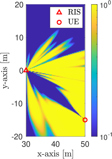
(a)

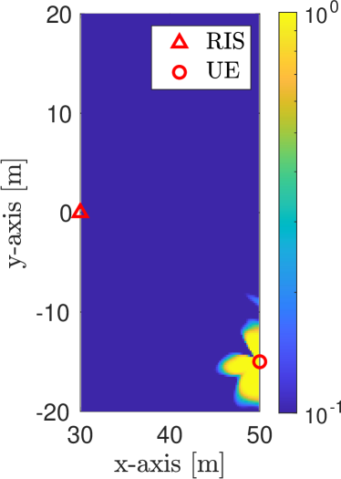
(b)

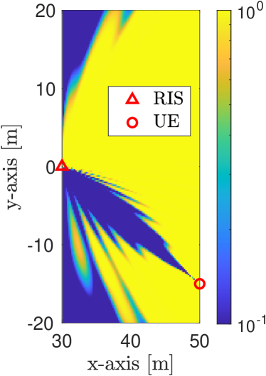
(c)

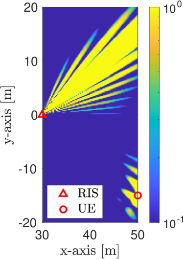
(d)

Figure 3: Detection probabilities with the respect to the SP locations ($P_{\mathrm{Tx}}=20$ dBm, $T=20$, $\mathbf{x}_{\mathrm{U}}=[50,0,0]^{\top}$, $\mathbf{x}_{\mathrm{R}}=[30,0,0]^{\top}$): (a) UE-RIS-SP-UE with $\tilde{\bm{\omega}}_{\tilde{t}}^{\mathrm{rand}}$; (b) UE-SP-RIS-UE with $\tilde{\bm{\omega}}_{\tilde{t}}^{\mathrm{rand}}$, (c) UE-RIS-SP-UE with $\tilde{\bm{\omega}}_{\tilde{t}}^{\mathrm{direct}}$; and (d) UE-SP-RIS-UE with $\tilde{\bm{\omega}}_{\tilde{t}}^{\mathrm{direct}}$. We set $\tilde{\bm{\omega}}_{\tilde{t}}^{\mathrm{direct}}=(\mathbf{a}_{\mathrm{U}}(\bm{\phi}_{0})\odot\mathbf{a}_{\mathrm{U}}(\bm{\phi}))^{*}$, where $\bm{\phi}$ is the angle at RIS to the point $[50,15,0]^{\top}$.

Figure 4: Complementary cumulative distribution function of the detection probabilities $P_{\mathrm{U}}$ for UE-RIS-SP-UE, UE-SP-RIS-UE, UE-SP-UE paths with RIS configurations that are random $\tilde{\bm{\omega}}_{\tilde{t}}^{\mathrm{rand}}$ or directional $\tilde{\bm{\omega}}_{\tilde{t}}^{\mathrm{direct}}$.

Figure 5: GOSPA distances of SP sensing, with the directional and random precoders at the UE during the $T_{1}$ transmissions.

VI-B Results and Discussions

VI-B1 Adaptive Detection Probability

Fig. 3 depicts the DPs with the different SP locations. If we use $\tilde{\mathbf{f}}_{k,\tilde{t}}=\mathbf{a}^{*}_{\mathrm{U}}(\bm{\theta}_{k,0})/\|\mathbf{a}_{\mathrm{U}}(\bm{\theta}\|$ (i.e., directional precoder to the RIS), there is a region between RIS to UE, where SPs are not detectable, as shown in Fig. 3a–Fig. 3c, where Fig. 3a applies random RIS configurations, while Fig. 3c applies directional RIS configurations (i.e., $\tilde{\bm{\omega}}_{\tilde{t}}^{\mathrm{direct}}=(\mathbf{a}_{\mathrm{U}}(\bm{\phi}_{0})\odot\mathbf{a}_{\mathrm{U}}(\bm{\phi}_{l}))^{*}$). This occurs because the combiner $\mathbf{W}_{\perp}^{\mathrm{H}}$ is applied to extract the UE-RIS-SP-UE signal and reject the UE-RIS-UE signal. In other area, the DP is high, due to the high-gain directional UE precoding, and array gain due to the $N_{\mathrm{U}}-1$-dimensional observation. On the other hand, if we use a UE beam with null to the RIS, i.e., random precoders with $\tilde{\mathbf{f}}_{k,\tilde{t}}^{\mathrm{H}}\mathbf{a}_{\mathrm{U}}(\bm{\theta}_{k,0})=0$, the resulting DP is shown in Fig. 3b–Fig. 3d. The UE-SP-RIS-UE path is illuminated with low gain random UE precoders and provides only a scalar observation after combining. When using the directional RIS phase configurations, the detectable region from RIS to the point point $[50,15,0]^{\top}$ is larger than that with random RIS configuration $\tilde{\bm{\omega}}_{\tilde{t}}^{\mathrm{rand}}$. We omit the DPs of the UE-SP-UE signals since they are approximately equal to 1. Fig. 4 shows the complementary cumulative distribution function (CCDF) of DPs for all combinations of different SPs locations and UE trajectories. We see that lower DPs are achieved in the double-bounce signals, compared to the UE-SP-UE signal, due to the severe path loss of RIS reflection. We achieved higher DPs in the UE-RIS-SP-UE, compared to the UE-SP-RIS-UE, due to $N_{\mathrm{U}}-1$ beams by the combining matrix $\mathbf{W}_{\perp}\in\mathbb{R}^{N_{\mathrm{U}}-1\times N_{\mathrm{U}}}$. Thanks to the directional RIS phase $\tilde{\bm{\omega}}_{\tilde{t}}^{\mathrm{direct}}$, we obtain higher DPs for the UE-RIS-SP-UE and UE-SP-RIS-UE signals. For a more in-depth discussion on the detection performance, we refer to Appendix B.

VI-B2 Sensing

Fig. 5 shows the sensing performance. The solid black curves with the square markers indicate the RIS-sensing performance by the PMB filter given the measurement $\mathcal{Z}_{k}^{\mathrm{D}}$ and $\mathcal{Z}_{k}^{\mathrm{O}}$; solid blue curves with triangle markers indicate the NRIS-sensing performance given the measurement $\mathcal{Z}_{k}^{\mathrm{N}}$; and solid red curves with ‘x’ markers indicate the performance of the fusion of RIS- and NRIS-sensing. The PMB posteriors for RIS- and NRIS-sensing are fused, merged into one map. With the directional precoder $\tilde{\mathbf{f}}_{k,\tilde{t}}=\mathbf{a}^{*}_{\mathrm{U}}(\bm{\theta}_{k,0})/\|\mathbf{a}_{\mathrm{U}}(\bm{\theta}\|$ during the $T_{1}$ transmissions, the SP GOSPA distances gradually decrease as the number of observable SPs via double-bounce signals increases over time steps while the SPs via the UE-SP-UE are always observable. In addition, the measurement noise covariances of the double-bounce signals are higher than the UE-SP-UE signal, due to the severe path loss. Therefore, the RIS-sensing performance is worse than the NRIS-sensing. To show the importance of the directional UE precoders, we see that with random UE precoders during the $T_{1}$ transmissions, the SPs are rarely sensed via double-bounce signals, leading to poor GOSPA.

VII Conclusions

We presented a RIS-enabled passive object sensing framework with a monostatic sensing UE and several passive objects. This problem is shown to be challenging due to the multiple observations of each objects, via both single- and double-bounce paths. Detection probabilities for different paths and signals were derived and used in the observation system and PMB filter. Using the expressions of the detection probabilities, we analyzed the impact of precoder and the RIS. Sensing methods for data association and fusion were proposed and evaluated. Obtained results demonstrate that double-bounce paths provided limited information in addition to single-bounce paths, due to severe path loss of RIS reflection.

Appendix A Channel Parameters

We define the channel parameters as follows: $\tau_{k,0}=2\lVert\mathbf{x}_{\mathrm{U},k}-\mathbf{x}_{\mathrm{R}}\rVert/c$, $\tau_{k,l}=(\lVert\mathbf{x}_{\mathrm{U},k}-\mathbf{x}_{\mathrm{R}}\rVert+\lVert\mathbf{x}^{l}-\mathbf{x}_{\mathrm{R}}\rVert+\lVert\mathbf{x}_{\mathrm{U},k}-\mathbf{x}^{l}\rVert)/c$, $\bar{\tau}_{k,l}=2\lVert\mathbf{x}_{\mathrm{U},k}-\mathbf{x}^{l}\rVert/c$, $\phi_{k,0}^{\mathrm{az}}=\mathrm{atan2}(y_{\mathrm{UR}},x_{\mathrm{UR}})$, $\phi_{k,0}^{\mathrm{el}}=\mathrm{asin}(z_{\mathrm{UR}},\lVert\mathbf{x}_{\mathrm{UR}}\rVert)$, $\phi_{k,l}^{\mathrm{az}}=\mathrm{atan2}(y_{\mathrm{SR}}^{l},x_{\mathrm{SR}}^{l})$, $\phi_{k,l}^{\mathrm{el}}=\mathrm{asin}(z_{\mathrm{SR}}^{l},\lVert\mathbf{x}_{\mathrm{SR}}^{l}\rVert)$, $\theta_{k,0}^{\mathrm{az}}=\mathrm{atan2}(y_{\mathrm{RU}},x_{\mathrm{RU}})$, $\theta_{k,0}^{\mathrm{el}}=\mathrm{asin}(z_{\mathrm{RU}},\lVert\mathbf{x}_{\mathrm{RU}}\rVert)$, $\theta_{k,l}^{\mathrm{az}}=\mathrm{atan2}(y_{\mathrm{SU}}^{l},x_{\mathrm{SU}}^{l})$, $\phi_{k,l}^{\mathrm{el}}=\mathrm{asin}(z_{\mathrm{SU}}^{l},\lVert\mathbf{x}_{\mathrm{SU}}^{l}\rVert)$, where $\mathbf{x}_{\mathrm{UR}}=\mathbf{O}_{\mathrm{R}}^{\top}(\mathbf{x}_{\mathrm{U},k}-\mathbf{x}_{\mathrm{R}})$, $\mathbf{x}_{\mathrm{SR}}^{l}=\mathbf{O}_{\mathrm{R}}^{\top}(\mathbf{x}^{l}-\mathbf{x}_{\mathrm{R}})$, $\mathbf{x}_{\mathrm{RU}}=\mathbf{O}_{\mathrm{U}}^{\top}(\mathbf{x}_{\mathrm{R}}-\mathbf{x}_{\mathrm{U},k})$, $\mathbf{x}_{\mathrm{SU}}^{l}=\mathbf{O}_{\mathrm{U}}^{\top}(\mathbf{x}^{l}-\mathbf{x}_{\mathrm{U},k})$. Here, $\mathbf{O}_{{\mathrm{D}}}^{\top}$ is the rotation matrix that rotates global to local coordinates at UE, and similarly for the $\mathbf{O}_{{\mathrm{R}}}^{\top}$ and the RIS [25].

Appendix B Link Budget Analysis

To understand the fundamental limits on the RIS signals for monostatic sensing, we investigate path losses for the different signals i)-iv), determined by the received to transmitted power ratio. To this end, we consider a scenario where the UE and SP are towards the broadside of the RIS and focus only on the power, without accounting for beamforming or combining at the UE. We define $d_{\mathrm{UR}}=\lVert\mathbf{x}_{\mathrm{U}}-\mathbf{x}_{\mathrm{R}}\rVert$, $d_{\mathrm{US}}=\lVert\mathbf{x}_{\mathrm{U}}-\mathbf{x}\rVert$, and $d_{\mathrm{RS}}=\lVert\mathbf{x}_{\mathrm{R}}-\mathbf{x}\rVert$. With transmit power $P_{\mathrm{T}}$, We will denote the received powers for the different signals i)-iv) are respectively denoted by $P_{\mathrm{R}}^{\mathrm{R}}$, $P_{\mathrm{R}}^{\mathrm{D}}$, $P_{\mathrm{R}}^{\mathrm{O}}$, and $P_{\mathrm{R}}^{\mathrm{N}}$, given by

$$P_{\mathrm{R}}^{\mathrm{R}} =\frac{P_{\mathrm{T}}G_{\mathrm{RIS}}^{\prime}\lambda^{2}A_{\mathrm{RIS}}}{(4\pi)^{2}d_{\mathrm{UR}}^{4}},$$ (18)

$$P_{\mathrm{R}}^{\mathrm{D}} =P_{\mathrm{R}}^{\mathrm{O}}=\frac{P_{\mathrm{T}}G_{\mathrm{RIS}}\lambda^{2}S_{\mathrm{RCS}}A_{\mathrm{RIS}}}{(4\pi)^{4}d_{\mathrm{US}}^{2}d_{\mathrm{UR}}^{2}d_{\mathrm{RS}}^{2}},$$ (19)

$$P_{\mathrm{R}}^{\mathrm{N}} =\frac{P_{\mathrm{T}}\lambda^{2}S_{\mathrm{RCS}}}{(4\pi)^{3}d_{\mathrm{US}}^{4}},$$ (20)

where $A_{\mathrm{RIS}}=(\lambda/4)^{2}$ is the area of a RIS element, $G_{\mathrm{RIS}}=\mathbb{E}\left\{|\mathbf{a}^{\top}(\bm{\phi}_{0})\bm{\Omega}\mathbf{a}(\bm{\phi}_{l})|^{2}\right\}$ is the RIS gain for the double-bounce paths, in which $\bm{\phi}_{l}$ is the AoA/AoD from the SP, and $G^{\prime}_{\mathrm{RIS}}=\mathbb{E}\left\{|\mathbf{a}^{\top}(\bm{\phi}_{0})\bm{\Omega}\mathbf{a}(\bm{\phi}_{0})|^{2}\right\}$ is the RIS gain for the UE-RIS-UE path. In this setup, $\bm{\phi}_{l}=\bm{\phi}_{0}$, so $G_{\mathrm{RIS}}=G^{\prime}_{\mathrm{RIS}}$. In the case of directional RIS configurations $G_{\mathrm{RIS}}=N_{\mathrm{R}}^{2}$, while for random configurations $G_{\mathrm{RIS}}=N_{\mathrm{R}}$.

We now plot the path loss $P_{\mathrm{R}}/P_{\mathrm{T}}$ for each of the paths in Fig. 6. We consider 2 scenarios: in scenario (a) the SP is between the UE and the RIS, so that $d_{\mathrm{RS}}=\rho_{\mathrm{S}}d_{\mathrm{UR}}$, for $\rho_{\mathrm{S}}\in(0,1)$; in scenario (b) the UE is between the SP and the RIS, so that $d_{\mathrm{RU}}=\rho_{\mathrm{U}}d_{\mathrm{RS}}$, for $\rho_{\mathrm{U}}\in(0,1)$. We set $d_{\mathrm{UR}}=30~{}\mathrm{m}$ for scenario (a) and $d_{\mathrm{RS}}=30~{}\mathrm{m}$ for scenario (b), while other parameters are as in Section VI. We observe that in scenario (a) (see Fig. 6a), the single bounce path UE-SP-UE is nearly always the strongest (with path loss above $-114$ dB). Under random configurations, the UE-RIS-UE path has a loss of around $-150$ dB, while the double-bounce path has a loss that varies from $-130$ dB (SP close to RIS or UE) to $-160$ dB (SP in the middle). With directional RIS profiles all RIS paths are boosted by $10\log_{10}(2,500)=34$ dB, providing a gain over the UE-SP-UE path with about $16$ dB when the SP is very close to the RIS. Moreover, in both cases of RIS configurations, the path UE-RIS-UE is generally stronger than the double-bounce paths, leading to severe interference (which was mitigated in this work by UE beamforming and combining). In scenario (b), the curves for UE-SP-UE and UE-RIS-SP-UE are the same as in scenario (a), due to the symmetry of the path loss. The difference lies in the UE-RIS-UE path, which is stronger when the UE is close to the RIS, but again nearly always dominates and thus interferes with the double-bounce paths.

(a) SP between RIS and UE

(b) UE between RIS and SP

Figure 6: Path losses where in (a) $d_{\mathrm{RS}}=\rho_{\mathrm{S}}d_{\mathrm{UR}}$ while in (b) $d_{\mathrm{RU}}=\rho_{\mathrm{U}}d_{\mathrm{RS}}$.

References

- [1] A. Liu et al., “A survey on fundamental limits of integrated sensing and communication,” IEEE Commun. Surv. Tutor., vol. 24, no. 2, pp. 994–1034, 2022.
- [2] S. P. Chepuri et al., “Integrated sensing and communications with reconfigurable intelligent surfaces,” arXiv preprint arXiv:2211.01003, 2022.
- [3] H. Kim et al., “RIS-enabled and access-point-free simultaneous radio localization and mapping,” arXiv preprint arXiv:2212.07141, 2022.
- [4] E. Björnson et al., “Reconfigurable intelligent surfaces: A signal processing perspective with wireless applications,” IEEE Signal Process. Mag., vol. 39, no. 2, pp. 135–158, Mar. 2022.
- [5] H. Zhang et al., “Toward ubiquitous sensing and localization with reconfigurable intelligent surfaces,” Proc. IEEE, vol. 110, no. 9, pp. 1401–1422, Sep. 2022.
- [6] Z. Yang et al., “MetaSLAM: Wireless simultaneous localization and mapping using reconfigurable intelligent surfaces,” IEEE Trans. Wireless Commun., 2022.
- [7] A. Aubry et al., “Reconfigurable intelligent surfaces for N-LOS radar surveillance,” IEEE Trans. Veh. Technol., vol. 70, no. 10, pp. 10 735–10 749, 2021.
- [8] S. Buzzi et al., “Radar target detection aided by reconfigurable intelligent surfaces,” IEEE Signal Process. Lett., vol. 28, pp. 1315–1319, 2021.
- [9] ——, “Foundations of MIMO radar detection aided by reconfigurable intelligent surfaces,” IEEE Trans. Signal Process., vol. 70, pp. 1749–1763, 2022.
- [10] X. Wang et al., “Joint waveform design and passive beamforming for RIS-assisted dual-functional radar-communication system,” IEEE Trans. Veh. Technol., vol. 70, no. 5, pp. 5131–5136, 2021.
- [11] R. P. Sankar et al., “Joint communication and radar sensing with reconfigurable intelligent surfaces,” in Proc. IEEE SPAWC, 2021.
- [12] G. C. Alexandropoulos et al., “Hybrid reconfigurable intelligent metasurfaces: Enabling simultaneous tunable reflections and sensing for 6G wireless communications,” arXiv preprint arXiv:2104.04690, 2021.
- [13] Á. F. García-Fernández et al., “Poisson multi-Bernoulli mixture filter: Direct derivation and implementation,” IEEE Trans. Aerosp. Electron. Syst., vol. 54, no. 4, pp. 1883–1901, Aug. 2018.
- [14] H. Kim et al., “PMBM-based SLAM filters in 5G mmWave vehicular networks,” IEEE Trans. Veh. Technol., vol. 71, no. 8, pp. 8646–8661, Aug. 2022.
- [15] G. Battistelli et al., “Consensus CPHD filter for distributed multitarget tracking,” IEEE J. Sel. Topics Signal Process., vol. 7, no. 3, pp. 508–520, Jun 2013.
- [16] R. Mahler, Statistical Multisource-Multitarget Information Fusion. Norwood, MA, USA: Artech House, 2007.
- [17] K. Keykhosravi et al., “RIS-Enabled SISO localization under user mobility and spatial-wideband effects,” IEEE J. Sel. Topics Signal Process., Aug. 2022.
- [18] ——, “RIS-enabled self-localization: Leveraging controllable reflections with zero access points,” in Proc. IEEE ICC, 2022.
- [19] S. Palmucci et al., “RIS-aided user tracking in near-field MIMO systems: Joint precoding design and RIS optimization,” arXiv preprint arXiv:2212.07333, 2022.
- [20] H. Wymeersch et al., “Adaptive detection probability for mmWave 5G SLAM,” in Proc. 6G SUMMIT, Mar. 2020.
- [21] K. Panta et al., “Novel data association schemes for the probability hypothesis density filter,” IEEE Trans. Aerosp. Electron. Syst., vol. 43, no. 2, pp. 556–570, Apr. 2007.
- [22] I. Arasaratnam et al., “Cubature Kalman filters,” IEEE Trans. Autom. Control, vol. 54, no. 6, pp. 1254–1269, Jun. 2009.
- [23] M. Fröhle et al., “Decentralized Poisson multi-Bernoulli filtering for vehicle tracking,” IEEE Access, vol. 8, pp. 126 414–126 427, Aug. 2020.
- [24] X. R. Li et al., “Survey of maneuvering target tracking. Part I. Dynamic models,” IEEE Trans. Aero. Electron. Syst., vol. 39, no. 4, pp. 1333–1364, Oct. 2003.
- [25] Z. Abu-Shaban et al., “Error bounds for uplink and downlink 3D localization in 5G millimeter wave systems,” IEEE Trans. Wireless Commun., vol. 17, no. 8, pp. 4939–4954, Aug. 2018.
- [26] W. Tang et al., “Wireless communications with reconfigurable intelligent surface: Path loss modeling and experimental measurement,” IEEE Trans. Wireless Commun., vol. 20, no. 1, pp. 421–439, Jan. 2020.
- [27] A. S. Rahmathullah et al., “Generalized optimal sub-pattern assignment metric,” in Proc. 20th Int. Conf. Inf. Fusion (FUSION), Xian, China, Jul. 2017, pp. 1–8.