botcap, captionskip=2pt, mincapwidth=2in, framebg=1 1 1, framefg=0 0 0, framerule=0pt, framesep=0pt,
Explainability of Text Processing and Retrieval Methods: A Critical Survey
Abstract.
Deep Learning and Machine Learning based models have become extremely popular in text processing and information retrieval. However, the non-linear structures present inside the networks make these models largely inscrutable. A significant body of research has focused on increasing the transparency of these models. This article provides a broad overview of research on the explainability and interpretability of natural language processing and information retrieval methods. More specifically, we survey approaches that have been applied to explain word embeddings, sequence modeling, attention modules, transformers, BERT, and document ranking. The concluding section suggests some possible directions for future research on this topic.
1. Introduction
Given the volume of information that we routinely encounter, we have become acutely dependent on technology that attempts to process the available information, classify it on the basis of diverse criteria, select useful information from this barrage, and present it in a form that is easy to consume and assimilate. It is not enough for such technology to be good at what it does: as humans, we would ideally also like to understand why our tools behave the way they do. Naturally, a substantial body of research has focused on methods for providing high-level, human-understandable interpretations or explanations of the inner workings of, as well as the results produced by, information processing tools and technologies.
Upto about 10 years ago, commonly used information processing tools generally extracted a feature vector — a list of features along with their associated numerical weights — from the form in which the information was initially provided: structured or unstructured text, images, audio, video, etc. These features typically corresponded to human-understandable properties or attributes of the original information. We confine our discussion in this article to textual information only. For text, features would include words and phrases occurring in the text, their counts, morphology, parts of speech, and various grammatical structures appearing in the text. These features were chosen on the basis of linguistic considerations; they were, in a sense, interpretable by design. A number of studies (some of which are discussed in more detail in Section 9) did focus on understanding feature weights, their behaviour, and the mathematical / statistical models underlying their computation and use, but they were not explicitly designated as explainability / intepretability studies.
Over the past few years, advances in Deep Machine Learning (ML) techniques have revolutionised the state of the art in textual information processing (and, of course, in a number of other areas). However, these improvements have come at a cost: text is no longer simply represented in terms of easily interpretable features. Instead, early in the information processing pipeline, text is converted to so-called “dense” vectors in ; the dimensions of this space are no longer easily understood, even in isolation. This representation is then processed by ML systems that have large and complex architectures, involving many parameters, often numbering in the millions. As a consequence, in recent times, the research community has devoted a good deal of attention to providing high-level, intuitive explanations of these models and methods.
Thus, this seems to be an appropriate time to present an organised summary of the major research efforts in the area of explainability in textual information processing and retrieval. Indeed, several such general surveys have already been published (Søgaard, 2021; Madsen et al., 2022; Zini and Awad, 2022; Anand et al., 2022), in addition to more specialised surveys, such as (Belinkov and Glass, 2019; Dufter et al., 2022). Our objective is to complement these existing surveys by discussing more recent work in areas already covered there, and by focussing on areas not addressed by them. Before discussing these surveys in more detail in Section 2, we first briefly describe how we collected the set of papers summarised in this survey.
1.1. Scope
Text processing and retrieval problems are studied by researchers from the Information Retrieval (IR) and Natural Language Processing (NLP) communities, as well as from the broader Machine Learning / Deep Learning (DL) communities. Thus, to ensure comprehensive coverage of explainability and interpretability studies relating to IR and NLP, we identified papers from a wide range of highly-regarded venues including SIGIR, CIKM, WSDM, WWW, the ACL family of conferences and journals, AAAI, ICML, ICLR, NeurIPS, FAccT and IPM (Information Processing & Management). From the longlisted set of papers, a subset of 41 papers was selected for discussion in this article.
While assessing and summarising research results in an empirical discipline, it is important to keep in mind what datasets were used for validation, as well as their limitations, if any. Accordingly, in addition to discussing the method(s) adopted in each study, we make it a point to include details about the datasets that were used for experimental evaluation.
Organization of the survey: The remainder of this survey is organised as follows. Section 2 lists existing surveys that cover explainability in textual IR and NLP, and describes the relation between them and the current article. Section 3 introduces the basic terminology used in the literature on explainability. Section 4 reviews some well-known approaches to explainability that are most commonly used as baselines in recent work. Sections 5 through 8 cover explainability for the various elements of deep text processing and retrieval pipelines, e.g., word embeddings, attention mechanisms, transformer architectures, and are intended as supplements to existing surveys (specifically those by Madsen et al. (2022) and Zini and Awad (2022)). Section 9 is devoted to a detailed discussion of explainable document / passage ranking, and is itself divided into subsections by topic. Within each of these sections and subsections, different studies have been discussed in chronological order. We conclude in Section 10 with a few research questions that we believe merit further investigation.
2. Related Work
In a recent monograph (Lin et al., 2021), Lin et al. provide a comprehensive survey of neural IR models, covering topics from multi-stage ranking architectures to dense retrieval techniques. The authors observe that IR models may be stratified into three fairly well-separated levels on the basis of effectiveness: transformer-based ranking strategies represent a definite advance over pre-transformer neural retrieval models, which in turn improve significantly over “traditional”111In this survey, we use this adjective to refer to all IR models (including relatively recently proposed ones) from the pre-neural era. statistical ranking models. An intuitive (but precise) grasp of what leads to these quantum jumps in effectiveness seems eminently desirable. This, along with a number of other factors, has led to much interest in the explainability of neural IR models. There has always been a substantial overlap between the IR and NLP communities. With the recent success of neural methods, the boundary between the disciplines has been blurred even further. Not surprisingly, therefore, research in explainable IR (ExIR) is significantly influenced by similar research in NLP, which in turn draws heavily from explainability studies in ML in general.
Our search for a comprehensive summary of research on this broad subject led us to two recent articles that provide an overview of attempts to explain neural models for NLP (Madsen et al., 2022; Zini and Awad, 2022). In (Madsen et al., 2022), the main emphasis is on post-hoc222In Section 3, we provide a review of this and other basic terms commonly used in the context of interpretability / explainability. methods for interpreting neural NLP methods, while Zini and Awad (2022) focus on the explainability of word embedding vectors, recurrent neural networks (RNNs) and attention mechanisms.
This being an area of active research, a non-trivial body of work exists that has not been covered by the above surveys, either because the work was published later, or because its topic was outside the specific scope of the surveys. In particular, until very recently, there were no similar overviews addressing ExIR in detail. The current study started as an attempt to address that lacuna. In the last few weeks, Anand et al. (2022) have published an article focused on this specific topic. There is, inevitably, a good deal of overlap between this manuscript and Anand et al.’s, but we also cover a fair amount of work that is not discussed by them. Specifically, given that ExIR often draws inspiration from explainability for NLP, we start by reviewing (in Sections 5 through 8) recent work on Explainable NLP that was not covered by the earlier surveys (Madsen et al., 2022; Zini and Awad, 2022). Section 9 also covers some work that is not included in (Anand et al., 2022). Further, since our survey was prepared independently, we believe that Section 9 provides a somewhat different perspective on ExIR. In the rest of this section, we briefly discuss other related surveys that are either older, or have a scope that does not substantially overlap with ours.
Onal et al. (2018) cover early work in the field of Neural IR (papers published on or before 2016). The monograph by Mitra and Craswell (2018) — an attempt to “bridge the gap [between researchers with expertise in either IR or Neural Networks], by describing the relevant IR concepts and neural methods in the current literature” — covers more recent work (including some articles published in 2018). Both surveys predate the widespread use of transformer-based architectures for IR. Further, their focus is on the retrieval methods and models themselves, rather than on work that attempts to explain or interpret them.
To the best of our knowledge, Doshi-Velez and Kim (2017) were the first to attempt to formalise various notions related to interpretability in ML. Lipton (2018) also provides an exposition of the broader aspects of interpretability in ML and Artificial Intelligence (AI), and why it is challenging, especially in the modern scenario. Søgaard (2021) examines extant taxonomies of explainability methods, and carefully constructs a framework for organising them. The next section draws from these articles to build a glossary of common terms used in this area.
Belinkov and Glass (2019) focus specifically on explainable NLP, and cover studies that seek to understand what kinds of linguistic features are encoded by neural NLP models by analysing, for example, neural network nodes, and activations across different layers of deep neural networks. As mentioned above, many of the discussed methods were based on general interpretability approaches proposed by the ML community, often within the context of the Computer Vision / Image Processing problems. Signalling the growing interest in this area of research, Danilevsky et al. (2020) also provide an early overview of explainability for NLP, describing different explanation categories and approaches, as well as several visualization techniques. Lertvittayakumjorn and Toni (2021) focus on explanation as a tool for debugging NLP models, with humans in the loop.
As Transformer and BERT-based techniques were widely adopted in the IR/NLP community, several researchers focused on various aspects of BERT, from its knowledge-representation power to fine-tuning, pre-training, and over-parametrisation issues. Rogers et al. (2020) were the first to survey research in this category, and present a summary of “what we know about how BERT works.” The surveys discussed at the beginning of this section provide a more up-to-date summary of research in this broad area.
3. Basic Terminology
This section provides a glossary of some basic terminology used in the literature on Explainability and Interpretability.
Interpretability: We adopt the following definition given by Doshi-Velez and Kim (2017): interpretability is “the ability to explain or to present in understandable terms to a human”. In this article, we use the terms explainability and interpretability interchangeably.
Inherent interpretability: Some ML models, e.g., decision trees and sparse linear models, are regarded as inherently explainable, because it is relatively simple for a human to trace their inner workings. Of course, the notion of inherent explainability is itself the subject of much debate. For example, Moshkovitz et al. (2020) argue that even apparently well-understood methods with a single parameter, viz., -means and -medians clustering techniques may be regarded as “opaque”, because these methods define cluster boundaries on the basis of linear combinations of features, rather than a single feature value. More pertinent to our context is the debate on whether the attention mechanism can be construed as providing explanations. Section 7.1 discusses this debate in more detail.
Global vs. local interpretability: Global methods explain the overall behavior or decision of a model. Global explanations should apply to all possible (or most) input-output pairs for a given model. Naturally, such explanations are difficult to provide for complex models. On the other hand, a local explanation only seeks to explain a model’s decision for a given set of input instances.
Model agnostic explanations: are explanations that treat the explained model as a black box, without assuming anything about its internal architecture or parameters.
Post-hoc explanations: primarily seek to elucidate the output, rather than explain the inner workings of models. For example, visualising word embeddings using t-SNE (Van der Maaten and Hinton, 2008) are a form of post-hoc explanation: they do not explain why certain words are mapped to certain vectors, but they help humans to understand the correspondence between proximity in the semantic and vector spaces, once the vectors are generated (i.e., after the fact). Explanations by example (of the form: “Model predicts class for input instance because is ‘similar’ to training instances which were labelled ”) also fall within this category.
Rationales: A subset of input tokens that is important for the prediction of a model is termed a rationale. For example, a part of the input text that is small yet sufficient to correctly predict the sentiment of a sentence comprises a rationale (DeYoung et al., 2020) for a sentiment classification task / model.
4. Baseline Methods
Before moving to a detailed discussion of explainability research in IR/NLP, we review some important methods that are widely used as baselines against which more recent approaches are compared.
4.1. Local interpretable model-agnostic explanations (LIME)
A very popular post-hoc approach, LIME was introduced by Ribeiro et al. (2016). Let be a complex classifier whose output we want to explain for a given task on a given dataset. For each input instance , a set of slightly perturbed instances of is generated. For example, if is a text document, may be created by deleting random words from random positions in . The idea is to then train a simple classifier that closely approximates ’s behaviour on . Since no assumptions are made about , is model-agnostic. Further, is local since it mimics for the given instances; no claim is made about how close and are in general. In (Ribeiro et al., 2016), for example, a linear SVM was used to approximate an SVM with an RBF kernel for classifying text documents. The linear SVM was then used to understand the behaviour of its more complex variant.
4.2. Feature Attribution
The objective of feature attribution is to quantify the contribution of a particular feature towards the predictions made by a model. Several techniques for computing and visualising feature attribution scores have been proposed in the literature. Among the simplest feature attribution techniques is occlusion (Zeiler and Fergus, 2014; Li et al., 2016) (sometimes referred to as the leave one out method). This estimates the importance of a group of features by setting all these features to zero, and measuring the resulting decrease in prediction accuracy. Some other well-known feature attribution approaches are gradient based techniques, integrated gradients (Sundararajan et al., 2017), saliency maps (Simonyan et al., 2014) and deeplift (Shrikumar et al., 2017). A library implementing many of these important attribution algorithms for interpreting PyTorch models is available via https://captum.ai/.
4.2.1. Integrated Gradients (Sundararajan et al., 2017)
Integrated gradients identify important features by considering a given input feature vector along with a “baseline” (, say) that represents a very simple input. For example, if the input is an image, the baseline could be a black image; similarly, when studying word embeddings, the zero vector would be a possible baseline. We generate additional instances by linearly interpolating between the input instance and the baseline . Gradient values corresponding to the change in the output prediction for small changes in the input are computed over all the generated instances. The importance of the -th feature or dimension of is measured in terms of its integrated gradient, , which is mathematically defined as
where denotes the gradient of the prediction with respect to the -th dimension of .
4.2.2. Shapley
The Shapley value (Shapley, 2016) was originally proposed in 1952 in the context of Cooperative Game Theory to quantify the contribution of a player to the outcome of a game. Suppose a team of players participates in a game and receives a payout after playing the game. The central question addressed by Shapley involves distributing the payout to individual team members in a fair way, i.e., in accordance with their respective participation or contribution.
Lundberg and Lee (2017) first proposed the use of Shapley values to explain ML models: each feature may be regarded as a player, the model itself is the game, the prediction of the model is the payout, and the Shapley value for each feature measures its contribution towards the overall prediction. The time complexity of computing Shapley values according to the original formulation is exponential, since it involves examining all possible subsets of features. Lundberg and Lee (2017) formulate approximate versions, viz., Kernel SHAP, Tree SHAP (tree based approximation of SHAP), and Deep SHAP, that may be computed in reasonable time.
4.3. Probing
Probing classifiers are being widely adopted for analyzing deep neural networks. We take a neural model that was trained for a specific target task. We train a separate, usually simpler classifier on the final (or intermediate) representation generated by , to predict some specific linguistic property for the original input. If the new classifier performs well, we hypothesise that learned the linguistic property in question.
For example, given a sentence as the original input, one could run through a pre-trained version of BERT, and use a simple, single-layer feed forward network to assign Parts of Speech (POS) tags to each of the token representations generated by BERT. If the prediction accuracy of the POS tagger is high, we may claim that BERT’s representation encodes POS information. While a number of studies Köhn (2015); Gupta et al. (2015); Hupkes et al. (2018) have used probing methods to evaluate hypotheses like “neural models learn semantics” (or syntactic structures), Belinkov (2022) highlights drawbacks of probing methods, some of which are described below.
-
•
There are no general guidelines for selecting appropriate baselines for probing experiments, and by implication, for determining whether the new classifier performs “well enough” to support a particular hypothesis.
-
•
On a related note, the effect of the datasets used for the original and probing tasks has not been studied rigorously. The size, composition, and relationship between the original and probing datasets should be carefully investigated.
-
•
Structure of the probing classifier is important, whether it is simple or complex. There are also some work which deals with parameter free probing and suggest to report the accuracy complexity trade-off.
-
•
Probing frameworks may be able to associate some linguistic property with an intermediate representation, but it does not clearly establish what role, if any, that particular property played in the prediction of the original classifier.
5. Embeddings
Word embeddings are learned vector representations of words. Simple word embeddings are not context specific. The use of word embeddings is ubiquitous in NLP and IR applications. Pre-trained word embeddings are also used in the input layer of complex architectures, such as Transformers and BERT. However, the dimension of the embedding do not admit of any straightforward interpretation. In this section, we summarise recent work that seek to address this question.
5.1. Transformation of Embedding Spaces
A general approach to interpret embeddings involves applying a transformation to every word to project them into a space with interpretable dimensions. A description of some of these techniques can be found in (Zini and Awad, 2022, Section 5.2). Below, we summarise Densifier (Rothe et al., 2016), a variant of which is discussed in (Zini and Awad, 2022), and discuss a recent study that was not covered by earlier surveys.
Let denote the embedding matrix, i.e., the stack of embedding vectors of size , where is the number of words in the vocabulary. The objective of Densifier (Rothe et al., 2016) is to look for an orthogonal matrix such that the product is “interpretable” in the sense that the values of its first dimensions have a good correlation with linguistic features. More precisely, suppose and are two words; let be a linguistic feature. Intuitively, the objective function of Densifier looks for a unit vector such that is high (resp., low) when and differ (resp., agree) with regard to . In later work, Dufter and Schütze (2019) proposed a small modification to the objective function that allows them to obtain a closed-form analytic solution for that is hyper-parameter free. The transformed embeddings work well for lexicon induction and word analogy tasks. They used a simple linear SVM and Densifier as interpretability baselines.
The work by Mathew et al. (2020) takes a set of polar opposite antonym pairs given by users which is designated to be a pair of orthogonal pairs. The idea is to select corresponding subspace from the original pre-trained embedding vectors. Suppose and are a pair of antonyms, and let , be their corresponding embeddings. The new basis will be formed by . If we stack these basis vectors in a matrix form, say , and assume that original embedding of a word is and transformed embedding in this new subspace is . The pre-trained vectors are projected to this subspace formed by these antonym pairs as, . Therefore, the representation of can be obtained as . For example, (hard, soft) and (hot, cold) is an example of two opposite antonym pairs. We can obtain the transformation of the word ‘Alaska’ to this subspace. They used Word2Vec (Mikolov et al., 2013) and Glove (Pennington et al., 2014) based word embeddings.
The proposed framework POLAR was evaluated on a wide range of datasets: News Classification, Noun Phrase Bracketing, Question Classification, Capturing Discriminative Attributes, Word Analogy, Sentiment Classification, and Word Similarity tasks. Across most of the tasks, POLAR makes the vectors interpretable while retaining performance. Interpretability was measured by comparing the top 5 dimensions of words with Word2Vec and human annotators.
5.2. Changing Objective Function of Word Embeddings
One can change the loss function / cost function of a learning algorithm to incorporate specific objectives into it. Explicitly few components are added to the cost function to guide the learning process. A similar notion has been adapted to the literature of interpreting the dense representation of word embeddings. This helps to retain the underlying semantic structure of the embeddings simultaneously aligning the embedding dimensions to predefined concepts. In an earlier work by (şenel_utlu_şahinuç_ozaktas_koç_2021), the objective function of Glove (Pennington et al., 2014) embedding vectors was modified to incorporate a concept with a vector dimension. Concept word resources are provided as an external information to the learning algorithm. The cost function gives more weights to a embedding dimension if it belongs to a particular concept group. This encourages the training process to align the vector dimensions with the semantic space represented by the concept group. The size of embedding dimension and the number of concept word group were same.
However, it does not use the negative directions of the vectors. In a later work (Şenel et al., 2022) they used the positive and negative both direction of embedding vectors by changing the loss function of Glove and Word2Vec (Mikolov et al., 2013) vectors. Both the positive and negative directions are aligned to different concepts. In the cost function two components are added, one for positive concepts and another for the negative one. If a word belongs to positive concept group, it gets a higher weight, on the other hand, if it is from the negative word group it gets a negative weight. For example, the concept of ‘good’ and ‘bad’ is considered as opposites. Empirical evaluation was conducted on Word Similarity and Word Analogy tests. The embeddings were evaluated on three classification tasks, sentiment analysis, question classification, and news classification. In general, the average of word embedding vectors of input texts were considered and SVM classifier was used for training purpose.
6. Sequence Models
In this section we discuss interpretability of sequence models. A comprehensive discussion on the interpretability of RNNs and LSTMs can be found in (Zini and Awad, 2022). In this survey, we fill in the details with some specific LSTM based explainable techniques which attempt to identify what phrase level interactions are captured by LSTMs. Further we discuss some techniques based on hierarchical explanations.
Recall that, given a sequence of data, RNNs and LSTMs process one word at a time. We adopt the notation used in (Murdoch and Szlam, 2017; Murdoch et al., 2018). Let be a sequence of words, and let denote the word embedding vector for word . Then, the th LSTM cell and hidden state vectors are updated as:
| (1) | ||||
| (2) | ||||
| (3) | ||||
| (4) | ||||
| (5) | ||||
| (6) |
We assume that the input consists of tokens, each of which is a dimensional vector. The trainable weight matrices are and , the bias vectors are , and the dimension of the cell and hidden states is . The operator denotes element-wise multiplication. The sigmoid activated gates are called forget, input and output gates respectively. Initial cell and hidden state vectors i.e. and are initialized to 0. After processing the full sequence, a probability distribution over classes is computed as,
| (7) |
Below, we discuss some techniques all of which are of post-hoc interpretable paradigm.
6.1. Predictive Power of Individual Words
One approach for explaining the prediction of a neural classifier, for a given sequence of words, involves analysing the predictive power of the constituent words; i.e., the overall prediction of the classifier may be attributed to individual words that strongly predict a particular class. For example, when classifying the overall sentiment of a piece of text the presence of “delighted” indicates a strong positive sentiment. Extracting or identifying the discriminative nature of words is used as a technique to understand the behaviour of LSTM network.
Murdoch and Szlam (2017) explain the output of an LSTM network based on the influence of some specific words. Suppose we have a sequence {,,…,} of word embedding vectors . The idea is to extract key phrases from a trained LSTM network. The notion of phrases and words are used interchangeably here. Let denote the contribution of word for the prediction class . Intuitively, may be quantified upto and subtracting the previous ()th term. Formally they defined as,
| (8) |
In Equation 8, the terms and are decisions based on sequence upto and including the and word respectively. Therefore, the difference can be thought of as the contribution of the word to the decision. Recall from Equation 7, the output of an LSTM network can be decomposed in a following way,
| (9) | ||||
| (10) |
In a similar fashion , considering the forward propagation effect of LSTM’s forget gates between words and , can be defined as,
| (11) |
Here, the terms “words” and “phrases” are used interchangeably. The phrases are scored and ranked using above and values by averaging over all the documents. The predictive score (applying and individually) for a class of a phrase is calculated as the ratio of average contribution of that phrase to the prediction of class to class across all occurrences of that phrase.
As part of experimental evaluation mainly binary classification tasks were considered. Max predictive score () across the two classes were taken and the phrases were tagged with the label of that particular class. For example, the label for a phrase is considered to be if . To approximate the output of LSTM network a simple rule based classifier is used for string based pattern matching. Specifically, it starts with a document and a list of phrases sorted by predictive score . The idea is to search for each phrase in that document and once a phrase is matched it returns the label of the phrase. The algorithm stops once a best match is found. The experiments were conducted on SST and Yelp datasets for sentiment analysis task. The authors also used Wiki Movies for question answering task. For this task, given a question and document pair, their approach is to first encode the question with a LSTM model. The final encoded representation is augmented with the word embeddings of the individual words in the document. LSTM takes this encoded representation, and softmax classifier is used to predict whether a particular entity is an answer or not. Quantitative evaluations show that their simple rule based classifier can explain the output of LSTM network with the help of key phrases. However, there are some approximation error between LSTM and the pattern matching algorithm, i.e., LSTM was able to classify the sentiment whereas pattern matching algorithm fails here. Initial findings suggest that there are some broad context involved in the paragraph which helps LSTM to classify the sentences correctly. For example, the phrase “gets the job done” in a sentence like “Still, it gets the job done – a sleepy afternoon rental” got tagged as positive sentiment, however, the overall sentiment of the sentence is negative.
Murdoch et al. (2018) proposed a contextual decomposition (CD) based method for extracting interactions of an LSTM cell. For example, a phrase “used to be my favorite” present within a sentence is a negative statement, however their prior work (Murdoch and Szlam, 2017) fails to extract key phrase “used to be” as strongly negative. To overcome this sort of problem, in (Murdoch et al., 2018), any given phrase output of an LSTM is decomposedinto two parts, one that is contributed by that particular phrase () and another involving other factors (). Each output and cell state can be decomposed as,
| (12) | |||
| (13) |
The terms , represent the similar contributions to . Note that these and values are different than the previous work (Murdoch and Szlam, 2017). The idea is to recursively compute the decomposition and group the terms deriving from the phrase and involving other factors outside the phrase. Such a decomposition helps to identify the interactions between positive and negative sentiment of words. In the above example – “used to be my favorite”, a per word wise values were obtained with the help of heatmap. It is able to correctly identify “used to be” as strongly negative and “my favorite” as a positive sentiment. Intuitively as an isolation it shows the contributions made at each words to make the decision of the sentence. Experiments were conducted on binary sentiment analysis datatsets, Yelp and SST to demonstrate the workings of decomposition mechanism. The main objective was to investigate the phrase level and word wise CD scores, whether they can interpret different compositions and sentiments in a sentence. This type of decomposition helps to identify the negation in a phrase also. These per word / phrase level sentiments capture the internal dynamics of LSTM’s prediction. They used cell decomposition (Murdoch and Szlam, 2017), integrated gradients (Sundararajan and Najmi, 2020), leave one out (Li et al., 2016) and gradient times input as baselines to show the effectiveness of CD based approach.
6.2. Hierarchical Structure
There is a body of work aiming to identify groups of features that are most useful / have the greatest predictive power and use them in hierarchical manner to show the interactions between the features. In this context, features are simply individual words. Given the nature of language, we restrict our interest to groups of adjacent words / features.
Work by Singh et al. (2019) extends contextual decomposition (CD) based method in a hierarchical manner. They generalized the approach of computing CD scores to a generic deep neural network. In the work by Murdoch et al. (2018) CD scores were computed on each layers of LSTM. Here, generalized version computes CD score on each layer of the neural network as
| (14) |
where, is the input to the network and is the number of layers in the network. On each layer , is composed of two components, measuring the importance of the feature group present in the input and captures contributions of rest of the tokens in the input. For each layer, . One can measure on each layer what would be the score of and values (from the discussion in the earlier section (Murdoch et al., 2018)). The proposed method can be generalized to spatial domain with CNN based deep networks. CD decompositions for convolution, max-pooling, dropout, ReLU were discussed separately. As our survey is focused to text domain, we omit these details for brevity. To combine the group of words agglomerative contextual decomposition (ACD) was proposed. The structure of the algorithm looks analogous to agglomerative clustering. It starts by combining the CD scores computed on each features. The algorithm merges score of adjacent features in a bottom up manner by building a priority queue and inserting the words, phrases (similarly using pixels for images) and their contribution scores into it. They used SST, MNIST, and ImageNet datasets for hierarchical interpretation purpose. For texts, it tries to point out when interaction between two phrase makes an incorrect prediction. The ACD is shown to be robust to adversarial perturbations in CNN. These perturbations were conducted on input instances by adding a small amount of noise. ACD algorithm produces a similar hierarchical explanation for perturbed instances as compared to the original one. This hypothesizes that ACD captures essential parts of the input.
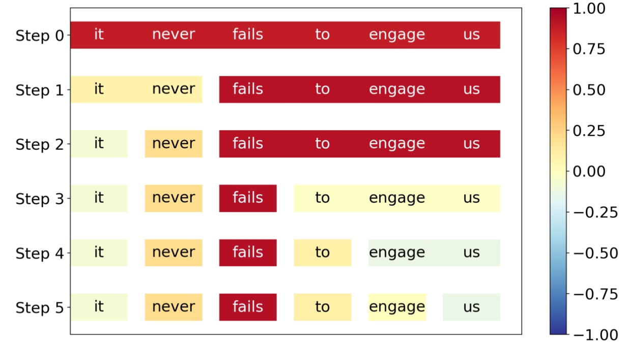
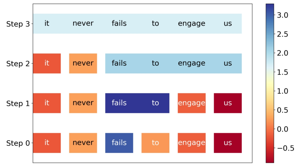
Another hierarchical explanations based model was proposed by Chen et al. (2020) with the same motivation as discussed above. Three types of neural classifiers, LSTM, CNN, and BERT were investigated on SST, IMDB datasets. The idea is at any point, the algorithm will pick a chunk of text and divide into two segments iteratively. Thus, there is two optimizations involved here, i.e., in each iteration which segment of text to pick and where to cut it. For the inner optimization i.e., to decide where to cut into two parts, they used shapley interaction index from (Lundberg et al., 2018). Subsequently for the outer optimization, they enumerate all the segments to pick the best possible text segment which has the smallest interaction index score. The contribution of a particular text segment ( are the starting and ending positions of a segment respectively) is obtained by measuring how far the prediction with respect to the prediction boundary. For text classification problem it is essentially the contribution made to a specific label . Figure 1 reproduced from (Chen et al., 2020) shows how this work differ from the earlier ACD based approach (Singh et al., 2019). In this example, hierarchical explanations provided bv (Chen et al., 2020) shows that LSTM makes an incorrect prediction as it missed the interactions between “never” and “fails”, whereas ACD is unable to capture this.
| Dataset | Descriptions | Task | Statistics |
|---|---|---|---|
| SST | Movie Reviews | Sentiment analysis | 6,920 / 872 / 1,821 |
| IMDB | Movie Reviews | Sentiment analysis | 25,000 / 4,356 |
| WikiMovies | Movie Domain | Question Answering | 100,000 |
| Yelp Review Polarity | Business Reviews | Sentiment analysis | 560,000 / 38,000 |
| M.RC | Reading Comprehension | Question Answering | 24,029 / 3,214 / 4,848 |
| SEMEVAL | Tweets | Classification | 6,000 / 2,000 / 20,630 |
| Ev.Inf | Biomedical Articles | Inference | 5,789 / 684 / 720 |
| AG | News | Classification | 102,000 / 18,000 / 7,600 |
| QQP | Quora Questions | Paraphrase | 364,000 / 391,000 |
| QNLI | Wikipedia | QA / Natural Language Inference | 105,000 / 5,400 |
| MRPC | News | Paraphrase | 3,700 / 1,700 |
| ADR Tweets | Twitter Adverse Drug Reaction | Classification | 16,385 / 4,123 |
| 20 Newsgroups | News | Classification | 1,426 / 334 |
| AG News | News | Classification | 60,000 / 3,800 |
| Diabetes (MIMIC) | Clinical Health | Classification | 7,734 / 1,614 |
| Anemia (MIMIC) | Clinical Health | Classification | 5,098 / 1,262 |
| CNN | News | Question Answering | 380,298 / 3,198 |
| bAbI (Task 1 / 2 / 3) | Supporting Facts | Question Answering | 10,000 / 1,000 |
| SNLI | Human-written Sentence Pairs | Natural Language Inference | 549,367 / 9,824 |
7. Attention
The attention mechanism, originally termed as an alignment model in the context of machine translation by Bahdanau et al. (2015), has been a key component in text processing using deep neural networks since it was proposed. The attention models used in the literature are of two types: additive attention (Bahdanau et al., 2015) and scalar dot product (Vaswani et al., 2017). We assume a generic model framework and notations (Jain and Wallace, 2019; Mohankumar et al., 2020).
Suppose, we have a sequence of tokens . The model inputs , containing one-hot vectors at each position of the words and is the vocabulary size. This sequence is passed over an embedding layer to get a dimensional representations of each tokens . Encoder module takes this representations and produces a – dimensional hidden states. Note that one can consider LSTM, RNN or any sequence modeling network as a choice for the encoder module. Formally, the encoded representation . In a similar way we can encode a query (e.g. hidden representation of a question in question answering task). A similarity function takes , and produces scalar scores. Attention scores can be computed as: = softmax(()), where . Context vectors are obtained by combining attention scores with the hidden states. There are mainly two common similarity functions i.e. the choice of , additive () = and scaled dot product () = , where , are learnable parameters.
Attention distributions can be considered as inherently explainable if there is a cause-effect relationship between higher attention and the model prediction. A higher weight implies greater impact towards the prediction of a model. In general attention based explanations are characterised as faithful and plausible (Mohankumar et al., 2020). If higher attention signifies a greater impact towards the model prediction then it is called as faithful explanation. To evaluate faithful explanation we need to understand the correlation between inputs and output. One of the popular evaluation techniques is to order the words based on the attention weights and compute the average number of tokens required to flip the decision of a prediction (Nguyen, 2018). On the other hand, the explanation is considered as plausible if their weights can be understood by human. We need humans to evaluate whether they are plausible explanation or not.
7.1. Debate on Whether Attention is Explanation or not?
Though attention was initially thought of as inherently explainable, Jain and Wallace (2019) claimed that attention weights do not provide explanation through series of experiments on a wide range of datasets, SST, IMDB, ADR Tweets, 20 Newsgroups, AG News, Diabetes, Anemia, CNN, bAbI, SNLI datasets. It uses additive and scalar dot product versions of attention. They showed that correlation between attentions and feature attribution scores (gradient based measure) are weak for BiLSTMs based neural network with the attention component. It also shows the counterfactual attention weights i.e. alternative attention distributions on a different set of tokens using attention permutation and adversarial attention distributions. With attention permutation technique, randomly attention weights were re-assigned to different tokens. The goal of the adversarial attention mechanism is to get different attention weights while having similar prediction accuracy. These attention weights also produce similar results compared to the original one. They argued that therefore one cannot reliably say attention weights are faithful explanation.
In another work, Wiegreffe and Pinter (2019), argued some assumptions made by the earlier work of Jain and Wallace (2019) which refutes that attention may not be a good predictor for explainability. Wiegreffe and Pinter have shown that if the attention weights are frozen to a uniform distribution, it performs as well as the original one for some datasets. Therefore they conclude that attention is not necessary for these tasks and can not be useful to support the claims made by earlier research. In (Jain and Wallace, 2019) they detached the attention module from the original network and used the attention score as an independent unit, however in this work they claimed that the attention module is not a standalone module; it is computed alongside with the whole network. Attention weights learned from the LSTM’s attention layer were used in a non-contextualized model. The LSTM layer was replaced with MLP having the learned attention weights perform much better than simply training a MLP. This shows that attention weights capture word-level architecture, suggesting that they are not arbitrary. An adversary network was also trained by them in the attempt to mimic the base network and make the attention distributions as divergent as possible. Specifically, the loss function was modified by minimizing the prediction score from the original model and making the attention distributions diverge from the base model. Empirical results show that it is difficult to learn a different attention distribution consistently across all training instances. Further, the performance is sometimes task dependent. All the experiments were conducted on binary classification tasks with LSTM architecture. The datasets include SST, IMDB, 20 Newsgroups, AG News, Diabetes, Anemia.
7.2. Sparse Attention
Some recent work has explored sparse attention (Martins and Astudillo, 2016; Malaviya et al., 2018) as a way to reduce computational cost. One can think that as these approaches attend to a fewer tokens, sparse attention could induce better interpretability. However, Meister et al. (2021) have shown that sparseness does not necessarily improve interpretability, suggesting that this issue needs more study. The authors use the sparsegen (Laha et al., 2018) projection function to make the attention distributions sparse. It uses parameters to control the degree of sparsity. Their main objective is to check how strongly are input tokens related to their co-indexed intermediate representations, i.e., how much input token influences on the magnitude of the intermediate representations. If they are strongly related then sparse attention can identify influential intermediate representations as well as the input tokens. Further they checked if those intermediate representations can be primarily linked to any part of the input. In order to do so, they proposed a normalized entropy of gradient based feature importance scores by considering the influence of input token to it’s intermediate representations. If this value is very low (say ) then a single part of the input uniquely influences the intermediate representation. Experiments with three classification tasks, namely, IMDB, SST, 20News (topic classification) on LSTM and Transformer based neural models suggest that the relationship between intermediate representations and input tokens is not one-to-one even when the attention is sparse. Overall, they found that adding sparsity to attention decreases plausibility. Further, compared to standard attention mechanism, sparse attention correlates less with other feature importance measures.
7.3. Changing the Loss Function
One approach to incorporate faithfulness inside a neural model is to change the objective or loss function of the model by adding a penalty term to it. This idea can also be used to change attention distributions, hidden states of sequence models.
Mohankumar et al. (2020) proposed the Orthogonal and Diversity based LSTM models. They observed that hidden states of vanilla LSTM models are very similar as they occupy a narrow cone inside a latent space. It produces similar prediction for diverse set of attention weights. This shows that the model output does not change much if we randomly permute attention weights. In orthogonal LSTM, hidden states of a LSTM model were orthogonalized using Gram–Schmidt process. For Diversity LSTM, an explicit reward factor for conicity measure was added into the loss function. Intuitively, it penalizes the hidden state vectors when they are similar i.e., when they occupy in a narrow cone. The conicity measure for a set of vectors is defined as:
High conicity measure signifies low diversity of hidden state vectors.
These two types of modified LSTM models were evaluated with twelve different datasets ranging from text classification, natural language inference, and paragraph detection to question answering. Empirical results show that conicity measure for Orthogonal and Diversity LSTM models were much less compared to the vanilla one. Rationales extracted from Diversity LSTM received more attention compared to vanilla LSTM and also length wise they are relatively short. This model is found to be more faithful to human and correlates well with the integrated gradient based model (Sundararajan et al., 2017). The attention distributions on punctuation marks are significantly reduced and gives better distribution on different parts-of-speech tags. Diversity based LSTMs give more attention to noun and adjectives compared to the vanilla one, where these parts-of-speech played an important role towards prediction of classification tasks (e.g. sentiment analysis).
In (Chrysostomou and Aletras, ), the authors modified the loss function to incorporate faithfulness inside the Transformer model. Word salience distributions were computed using TEXTRANK (Mihalcea and Tarau, ), a graph-based keyphrase extraction algorithm. It helps to learn more informative input tokens, by penalizing the model when attention distributions deviates from word salience distributions. Formally they used KL divergence between the attention distribution and salience distribution. Empirical results on several datasets, SST, AGNews, Evidence Information (EV.INF), MultiRC (M.RC), Semeval show that it provides better faithfulness compared to rationale extraction and input erasure.
8. Transformers and BERT
Recently, Transformers and BERT (Vaswani et al., 2017; Devlin et al., 2019) based deep neural models have been shown to be very effective for various IR and NLP tasks. There are a couple of papers just focusing on interpretability of BERT — BERTology (Rogers et al., 2020). Here, we provide a brief discussion on the understanding of BERT. A more rigorous and broad overview can be found in the work by Rogers et al. (2020), who categorize the research questions on explainability of BERT into three general classes:
-
•
What types of different linguistic knowledge does BERT capture?
-
•
What is BERT output sensitive to?
-
•
Some analysis and interpretation of the attention heads of BERT.
Their work (Rogers et al., 2020) covers several aspects of BERT and also discuss about some limitations of BERT succinctly. In brief it talks about what syntactic, semantic, world knowledge does BERT have. This was conducted via analysis of self-attention weights, probing classifiers with various BERT representations as input, and fill-in-the-blanks probing of masked language model. Localizing linguistic knowledge in the self-attention head, special tokens and the different layers of BERT were also covered in this work. Some optimization techniques and architecture choices of BERT and studies considering tweaking pre-training, fine-tuning were discussed here.
As expected, in general the large variant of BERT, with more layers and larger hidden states per layer, performs better than the base variant, but this phenomenon is not true always. For example, BERT-base model outperforms the larger version of it on subject-verb agreement (Goldberg, 2019) and sentence subject detection (Lin et al., 2019) tasks. Also, the limitations of BERT was also discussed i.e. what all information it does not capture. It has been shown that BERT cannot reason over the facts. Further, it struggles with numeric floating point numbers, do not create good representations of them. Also, it does perform on named entity replacements tasks.
We provide detail descriptions on some specific components and add a new angle, e.g. information flow inside BERT, which we describe in the following section.
8.1. Significance of Different Layers of BERT
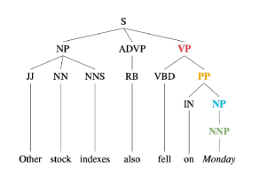
There have been a series of works discussing on what aspects do several layers of deep neural architectures encode. In general the idea is to obtain word representations trained from different layers and use them to determine what syntactic representations are captured with them by some probing task. In this thread an earlier work by (Blevins et al., 2018) demonstrated that RNN architectures encode some syntax without any explicit supervision. They probe with the word representations trained on different layers of RNN. Specifically, they used probing classifiers to predict parts-of-speech, parent, grandparent, great-grandparent in the constituent labels. Figure 2 shows an example of a constituency tree. They used English Universal Dependencies, CoNLL-2012, WMT02014 English-German, and CoNLL-2012 benchmark datasets for dependency, semantic role labeling, machine translation, and language modeling tasks for training the deep RNN models. Higher layers of RNNs encode less syntactic structure and contain representations in a more abstract sense. These observations were deduced from layer wise prediction accuracy obtained for various syntactic tasks.
In a similar spirit, the work by (Tenney et al., 2019a) proposed two types of scoring functions to evaluate the significance of different layers of BERT. First scoring function namely scalar mixing weight, is designed to evaluate the importance of individual layers. If there are layers, and the representation of layer is , then, we base the final decision on , tune on training data. The tuned was used to determine the importance of layers. Another scoring formula, namely cumulative score denotes how much accuracy measure F1 score changes for the introduction of a specific layer of BERT. Term can be used to measure the changes in F1 score observed while adding the layer. All the experimentation were evaluated on benchmark datasets English Web Treebank, SPR1, SemEval and OntoNotes 5.0 for eight different tasks — POS, constituents, dependencies, entities, semantic role labeling, coreference, semantic protocol roles, and relation classification. Similar to RNN architectures, in BERT also they observed the similar trend i.e, basic syntactic structures are captured earlier in the network, while the later layers are more suitable for semantics. Empirical results show that on average syntactic structures are more localizable but semantics are spread across different layers. However, for some challenging examples the model may not follow the above ordering. (Tenney et al., 2019a) cited the following examples to illustrate this phenomenon, S1: “he smoked toronto in the playoffs with six hits, seven walks and eight stolen bases…” S2: “china today blacked out a cnn interview that was …” In the first example (S1), the model initially thinks “Toronto” as city, therefore it tagged “Toronto” as GPE. After resolving the semantic role that “Toronto” is a thing “smoked” (ARG1), the entity of “Toronto” is modified to ORG. In this case, higher order task helps to identify / improve the lower order syntactic tasks. In the second example (S2), in the initial layers the model tags “today” as common noun, date. As this phrase is ambiguous, when it understands that “china today” is a proper noun, updates entity type of it and finally changed the semantic role of this also. In this specific example, the model does syntactic task first, then semantic task and later it does syntactic task as well as semantic task.
In (Jawahar et al., 2019) they mainly focused on identifying different types of linguistic structures captured by BERT base model. They conducted experiments to test several hypotheses and confirmed similar findings like the surface structures are encoded in the initial layers, whereas syntactic structures are captured in the middle layers, and semantic information is present in the upper layers by using various probing tasks (SentEval toolkit (Conneau and Kiela, 2018)), as discussed in Section 4.3. Specifically the experiments were conducted on ten probing tasks. The surface level features include sentence length, syntactic features include tree depth, and tense is considered as one of the semantic features (Conneau et al., 2018). It also captures dependency structures and higher layers are used for long range dependencies. A Tensor Product Decomposition Network (TPDN) (McCoy et al., 2019) was used to validate whether BERT implicitly learns to represent role-filler pairs. For example, in the task of copying a sequence of digits, one can represent a sequence as , where role is the position in a sequence and filler is the actual digits occupying the position. In this work they used position in a syntactic tree (path from root node to the word) as role and the word as the filler.
TPDN networks are used to approximate learned representations. In (McCoy et al., 2019) the authors assumed that for any specific role scheme if TPDN can be trained well to approximate the learned representation (by minimizing the mean squared error) of a neural network, the neural network is implicitly captuirng the role scheme.
8.2. Understanding Multi-headed Attention
In (Clark et al., 2019) attention maps of BERT-base (by extracting the attention distributions from BERT) were investigated. They probe each attention head for specific syntactic relations on dependency parsing datasets. It was observed that in earlier layers of BERT, there are heads that attend heavily on previous or next tokens. Attention to [SEP] is somewhat no-op for attention heads and attending this token more or less does not change BERT’s output. Broad attention (i.e., focus on many words) is perceived in the lower layer and in the [CLS] token of the last layer. Probing experiments show that although certain head focuses on some specific dependency relation (e.g. coreferent / antecedents, preposition / object, verb / direct object), it was not evident that individual heads attend to overall dependency structure.
Attention maps to some extent show coreference resolution also. They showed that attention maps have a thorough representation of English syntax which is distributed across multiple attention heads. Some attention heads behave similarly and heads within the same layer often have similar attention distribution.
The work by Pande et al. (2021) classified attention heads of BERT into different functional roles, which are:
-
•
local - tokens are attended in a small neighborhood of current token, generally next/previous tokens.
-
•
syntactic - attending tokens which are syntactically related to the current token.
-
•
delimiter - attending special tokens, i.e., [CLS] and [SEP].
-
•
block - tokens are attended within the same sentence contrary to the tokens in the sentences before or after the [SEP] token.
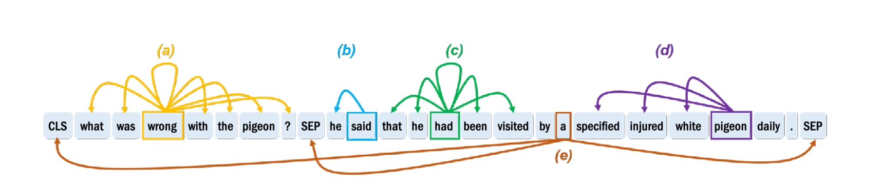
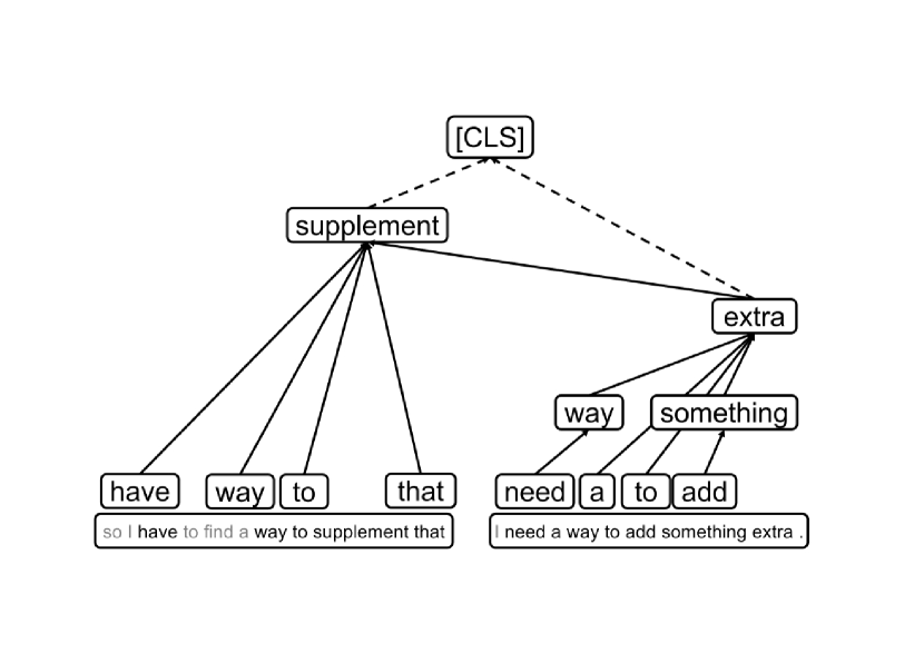
Figure 3 shows this categorization with a sample sentence. Attention sieve was defined by them as a set of tokens that will be attended to obtain the representation for a specific attention role. They proposed a sieve bias score as a ratio of average attention score given to the tokens in the sieve with the average attention given to all tokens in the input sequence. In case of syntactic attention head, the set of tokens from the input sequence that make up a sieve was identified by a dependency parser. For other heads it is quite straightforward to determine the sieve tokens. Additionally, they performed hypothesis tests to measure statistical significance on the mean of sieve bias score across all the input sequences. The null hypothesis was the mean of the sieve bias score across all the input sequences is less than or equal to some threshold. If the null hypothesis is rejected, the attention head is satisfying that specific functional role. Higher the threshold value, more stricter the classification rule for designating the particular head.
Experiments were conducted on QNLI (Wang et al., 2018) (QA Natural Language Inference), QQP (Wang et al., 2018) (paraphrase detection), MRPC (Dolan and Brockett, 2005) (paraphrase detection), and SST-2 (Socher et al., 2013) (sentiment analysis). They observed that middle layers of BERT are multi-skilled heads, later layers are specific to task. Syntactic heads are also local heads and delimiter heads overlap with other functional heads.
8.3. Power of Contextual Embedding
In (Tenney et al., 2019b), the advantage of contextualised embedding over the conventional word embeddings was discussed. An “edge probing” framework was established by them. A series of experiments on various NLP tasks such as, part-of-speech, constituent labeling, dependency, named entity labeling, semantic role labeling, coreference, semantic proto-role, relation classification was carried out by them. They used four popular contextual neural models, CoVe (McCann et al., 2017), ELMo (Peters et al., 2018), GPT (Radford and Narasimhan, 2018), and BERT to probe for the sub-sentence structure. They obtained context-independent representations from CoVe and ELMo. For CoVe it is the Glove vectors and in case of ELMo, the activations of the initial context-independent character-CNN layer was used. They observed that, contextualized embeddings capture syntax better and maintain a distant linguistic information over the non-contextualized ones, by comparing the micro-averaged F1 score for various probing tasks. Randomized version of ELMo where the weights are replaced with random orthonormal matrices was also considered. Results show that the randomized ELMo performs well on the probing suites, however with the learned representations of full ELMo almost 70% improvements can be achieved. Note that this is only an indication that the architecture of ELMo plays a significant role in the model’s performance, but does not explain what this role is.
8.4. Information Flow in BERT
Lu et al. (2021) observed that most of the information is passing through the skip connections of BERT. They showed that attention weights (Abnar and Zuidema, 2020) alone are not sufficient enough to quantify information flow. A gradient-based feature attribution (Sundararajan et al., 2017) method was discussed. Specifically, they introduced influence patterns as how gradient flows from input to output through skip connections, dense layers, etc. Gradient based influence patterns from input to output token can be constructed considering all possible paths using the chain rule. To reduce the computational overhead, they have used strategies to greedily add influential nodes from one layer to the adjacent layer. Path from input tokens to the output is considered a form of explanation. Experimental findings were conducted on subject word agreement and reflexive anaphora tasks. While previous methods only look into the aspects of attention weights, they do not discuss how information is traveling through the skip connections. In this work, they argued that BERT uses attention to contextualize information and skip connections to pass that information from one layer to another. Once contextualize step is finalized it relies more upon the skip connections. Experimental results also show that BERT is able to do negation in sentiment analysis tasks very well.
Another information interaction in the Transformer network was studied by Hao et al. through the lens of self-attention attribution (Sundararajan et al., 2017) based method. With feature attribution (integrated gradients) techniques, they identified important attention connections i.e. each pair of words in the attention heads of different layers. Intuitively, pair of words receive a high score if they contribute more to the final prediction. It was observed that a larger attention score between a pair of words may not contribute towards the final prediction.
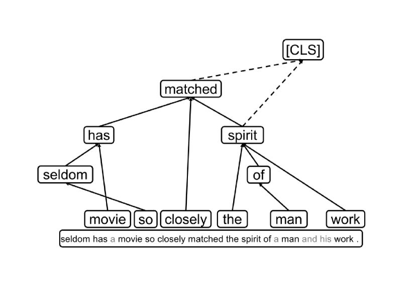
With the attribution scores of different heads, they pruned attention heads from different layers of BERT. Accuracy values do not change much if the heads with small attribution scores were pruned; however, heads with large attribution scores significantly impact the performance. In general, it was observed that two heads across each layer produce a good performance, and pruning the heads with average attention scores does not significantly affect performance. Further, important attention heads are highly correlated across different datasets. All the empirical results were conducted on MNLI, RTE, SST-2, and MRPC datasets. A heuristic algorithm was designed to demonstrate the information flow between input tokens inside the BERT layer. Figure 4 shows two instances, one from the MNLI dataset and another from the sentiment analysis dataset SST-2. For the first one, the interactions between input sentences try to explain the prediction. However, for the second example, although ‘seldom’, ‘movie’, and ‘man’ are more important words for the ‘positive’ sentiment to a human; the information flows presented by their approach do not aggregate to these tokens.
9. Document Ranking
Neural models for document ranking are generally divided into two categories: representation-based models and interaction-based models. Like traditional models, representation-based models also encode queries and documents as vectors; however, in contrast to the sparse vectors used by traditional approaches, these vectors are dense. On the other hand, interaction-based models capture complex interactions across query-term–document-term pairs. Transformer / BERT-based neural models are classified as representation-based, although there is some debate about this, which we discuss in Section 9.4. This section provides an overview of research efforts to explain the working of both categories of neural ranking methods, but first, we provide a brief review of some attempts to understand traditional IR models.
9.1. Understanding Traditional IR Models
Traditional IR systems typically represent documents using terms, i.e., single words (or word stems), and sometimes, additionally, groups of words that have special significance (these are often loosely referred to as phrases), along with their associated weights. The term weights (or feature weights) are calculated using either intuitive heuristics, or on the basis of various mathematical models. Traditional IR models may thus be regarded as explainable by design.
| Axiom Name | Axiom Nature | Axiom |
| TFC1 | Term frequency | favor a document with more occurrences of a query term |
| TFC2 | ensure that amount of increase in retrieval score of a document must decrease as more query terms are added | |
| TFC3 | favor a document matching more distinct query terms | |
| TDC | more discriminating query terms should get higher score | |
| TF-LNC | regulates the interaction between term frequency and document length | |
| LNC1 | Document Length | penalize a long document (assuming equal term frequency) |
| LNC2 | over-penalize a long document | |
| STMC1 (Fang and Zhai, 2006) | Semantic Constraints | retrieval score of a document increases as it contains terms that are more semantically related to the query terms. |
| STMC2 (Fang and Zhai, 2006) | avoid over-favoring semantically similar terms. | |
| STMC3 (Fang and Zhai, 2006) | retrieval score of a document increase as it contains more terms that are semantically related to different query terms. | |
| TSFC (Pang et al., 2017) | a document having higher exact match should get higher score if their semantic similarity score matches | |
| TP (Tao and Zhai, 2007) | Term Proximity | query terms appear in a closer proximity of a document should get higher retrieval score |
Fang et al., in (Fang et al., 2004) and a series of subsequent studies (Fang and Zhai, 2006; Fang et al., 2011), consolidated and formalised, within an axiomatic framework, the well-known constraints governing term-weighting models. This framework lays down a set of syntactic and semantic principles that can be used to reason why a particular document should be ranked above for a given query . It has been used to explain why certain retrieval models work better than other models, as well as to formulate improved versions of existing retrieval models (Clinchant and Gaussier, 2009b, a). Later efforts have focused on refining the framework by incorporating additional axioms (Tao and Zhai, 2007; Fang and Zhai, 2006), as well as expanding it to cover pseudo-relevance feedback methods (Clinchant and Gaussier, 2013). Table 2 lists some of the most popular axioms that have been mentioned in the literature. The page at https://www.eecis.udel.edu/~hfang/AX.html is an excellent resource on this topic.
While the axiomatic framework seems to be among the first approaches that is explicitly labeled with the ‘explainability’ tag, explaining or understanding the behaviour of Information Retrieval (IR) models has a long history. Singhal (1997) carefully examined traditional term-weighting formulae used in the Vector Space Model, explained why they do not work as well as more effective statistical models like BM25, proposed ways to modify the formulae in order to address these flaws, and demonstrated that the modified formulae do indeed yield significant improvements in retrieval effectiveness. In addition to retrieval from plain text, Singhal also considered noisy text collections, such as those generated by running Optical Character Recognition (OCR) systems on scanned images of documents, and explains why it is inadvisable to use cosine normalisation for such collections. Kamps et al. (2005) presented a similar study, undertaken in the context of retrieving XML elements from a collection of XML documents, that serves to explain the importance of length normalisation in XML retrieval. On a related note, Smucker and Allan (2006) compared two well-known smoothing techniques used in Language Modeling, and presented a different explanation for why Dirichlet smoothing outperforms Jelinek-Mercer smoothing, compared to the perspective provided by Zhai and Lafferty (2004).
9.2. Axiomatic Result Re-Ranking
Hagen et al. (2016) apply the axiomatic framework in a different way to improve retrieval effectiveness. Twenty three axioms (relating to term frequency, document length, lower bounds on term frequency, query aspects, semantic similarity, and term proximity) were used by them to analyse the documents in a given, initial ranked list. Each axiom induces relative orderings for document pairs; for example, axiom may be used to conclude that should be ranked higher than . These pairwise preferences were stored in matrices. An aggregation function for combining the twenty three orderings was learned using a set of training queries. Given a test query and a ranked list of initially retrieved documents, the axioms were again used to construct 23 pairwise preference matrices, which were combined using the learned aggregation function into a single preference matrix. A final ranking most consistent with this preference matrix was constructed using the Kwiksort algorithm (Ailon et al., 2008). Several baseline retrieval models333http://terrier.org/docs/v4.0/configure_retrieval.html were considered to empirically demonstrate the effectiveness of axiom based reranking strategies.
While this study does not seem to relate directly to explainability, it has practical significance for explainability in the following sense. To implement their approach, Hagen et al. formulated relaxed versions of some axioms. Axiom TFC1 (see Table 2), for example, induces an ordering on a document pair based on the term-frequencies of a query term in the two documents, provided the two documents are of equal length. This equality condition was replaced by an approximate equality constraint: axiom TFC1 was applied to a document pair if the relative difference in the lengths of the two documents was at most 10%. Similarly, for constraints related to the idf factor, idf values were rounded off to two decimal digits. A generalisation of the axioms from single term queries to multi term query was also proposed. For example, to apply TFC1 to multi term queries, they used the aggregate term frequency over all query terms. However, this ‘generalisation’ seems to directly contradict TFC3, which encapsulates the well-known principle that a match on different query terms is to be preferred to matches on a single term.
| Dataset | Collection Type | #Docs | #q | Pool Depth |
| MSMARCO passage (train) | question answering | 8,841,823 | 502,939 | Shallow |
| MSMARCO passage (dev) | 6,980 | Shallow | ||
| MSMARCO passage (test) | 6,837 | Shallow | ||
| MSMARCO document (train) | web | 3,213,835 | 367,013 | Shallow |
| MSMARCO document (dev) | 5,193 | Shallow | ||
| MSMARCO document (test) | 5,793 | Shallow | ||
| TREC 2019 DL passage | question answering | 8,841,823 | 43 | Depth |
| TREC 2019 DL document | web | 3,213,835 | 43 | Depth |
| TREC 2020 DL passage | question answering | 8,841,823 | 54 | Depth |
| TREC 2020 DL document | web | 3,213,835 | 45 | Depth |
| Robust | news | 528,155 | 249 | Depth |
| Clueweb09b | web | 50,220,423 | 200 | Depth |
Following Hagen et al. (2016), Völske et al. (2021) apply the axiomatic approach more directly, to provide post-hoc explanations of IR systems. As before, each axiom induces pairwise preferences over documents. The ranking generated by a particular retrieval model is approximated by an explanation model, which may be regarded as a weighted combination of these preferences. In the words of the authors, “(a) the explanation model’s parameters reveal the degree to which different axiomatic constraints are important to the retrieval model under consideration, and (b) the fidelity with which the initial ranking can be reconstructed can point to blind spots in the axiom set, which can help to uncover new ranking properties yet to be formalized.”
Altogether, twenty axioms were used in this study. Compared to the axioms used by Hagen et al. (2016), TFC2, LNC2, LB2, RSIM, QPHRA, ORIG, P-Rank were discarded. Instead, the authors considered two word embedding based variants of STMC1 and STMC2, corresponding to fastText word embeddings generated from either Wikipedia, or the Robust04 collection. The behaviour of three statistical models (BM25, TF-IDF, PL2) and five neural ranking models (MP-COS (Pang et al., 2016b), DRMM (Guo et al., 2016), PACRR-DRMM (McDonald et al., 2018), BERT-3S (Akkalyoncu Yilmaz et al., 2019), DAI-MAXP (Dai and Callan, 2019)) were studied using the MS MARCO and Robust04 collections. They observed that it is difficult to explain the relative ordering of two documents if they have similar retrieval scores, but a big difference in scores can be reliably explained in terms of the axioms. They also noted that explanation effectiveness was higher for the Robust04 collection, as compared to MS MARCO (in this study, explanation efficacy is measured in terms of how accurately the explanation model can replicate a retrieval model’s ranking).
9.3. Constructing Diagnostic Datasets
Following the trend of creating diagnostic datasets for NLP and Computer Vision applications, Rennings et al. (2019) used retrieval axioms to construct a similar dataset for IR from the WikiPassageQA (Cohen et al., 2018b) corpus. The idea is to investigate the extent to which various IR models satisfy axiomatic constraints. Four axioms were reformulated by relaxing the TFC1, TFC2, TDC and LNC2 axioms (ref. Table 2). The authors sampled query-document-pair triplets that satisfy the relaxed axioms from the dataset. For the relaxed version of LNC2, artificial documents had to be constructed. This diagnostic dataset was used to evaluate the axiomatic efficacy (the fraction of constraints that is satisfied by a retrieval model) of both traditional retrieval models (BM25 and LMDIR/QL), and neural models like DRMM (Guo et al., 2016), aNMM (Yang et al., 2016), Duet (Mitra et al., 2017) and MatchPyramid (Pang et al., 2016b). The authors observed that statistical models outperform the neural models in terms of satisfying the axiomatic constraints, but were significantly outperformed by DRMM and aNMM in terms of retrieval effectiveness. This suggests that the particular set of axioms considered in this study are not comprehensive enough to explain IR models.
Câmara and Hauff (2020) extended the above idea by considering additional axioms. Altogether a set of nine axioms (TFC1, TFC2, TDC, LNC1, LNC2, STMC1, STMC2, STMC3, TP) was used to evaluate the performance of DistilBERT (Sanh et al., 2019). Once again, empirical results show that DistilBERT significantly outperforms traditional query likelihood methods, but it does not perform as well in terms of axiomatic effectiveness. That this observation also applies to the semantic matching axioms, e.g., STMC1, is particularly counter-intuitive, and therefore, important. This suggests that the existing axioms, especially the semantic matching axioms, are not adequate for analysing BERT either, and need to be formulated more carefully.
On a different note, rather than applying the axiomatic framework to explain neural models, Rosset et al. (2019) have used this approach to ensure faster convergence of such models. Specifically, TFC1, TFC2, TFC3, TDC, and LNC (TF-LNC) constraints were used to create artificial, ‘perturbed’ documents. For example, given a document , a randomly sampled query term may be inserted at a random position in to create . According to TFC1, which states that we should give higher preference to a document that has more occurrences of query terms, should be more relevant compared to . These perturbed documents were added as additional training examples. Empirical results with the Conv-KNRM model (Dai et al., 2018) on the MS-MARCO (Nguyen et al., 2016) dataset show that the proposed approach makes Conv-KNRM converge faster, and also improves Mean Reciprocal Rank by 3%.
9.4. What knowledge do BERT based retrieval models possess?
This section looks at attempts to understand BERT based retrieval models, specifically monoBERT and ColBERT. Generally, these studies examine attention maps and query-document interactions, across different layers and heads, to understand what sort of knowledge BERT-based models encode internally that other statistical and previous neural ranking model do not.
Qiao et al. (2019) highlight the interaction-based, sequence-to-sequence nature of BERT using a few different versions of BERT-based rankers. A representation-based BERT model was designed by taking the individual [CLS] embeddings for both queries and documents, and computing the cosine similarity between them. Experimental evaluations were conducted on the MS MARCO (Nguyen et al., 2016) passage reranking and TREC Web Track ad hoc document ranking tasks. On both the datasets, the representation-based BERT model performed poorly, suggesting that BERT should not be used as a representation-based model. Interestingly, Qiao et al. observed that, while monoBERT outperforms the then-state-of-the-art neural IR models (K-NRM, Conv-KNRM) on MSMARCO, it fails to perform well for TREC adhoc ranking. They concluded that passage ranking for MSMARCO is more related to a question answering (QA) task, and therefore, better suited for a seq2seq model. Indeed, MSMARCO is basically a QA dataset, where precise matches are important. In contrast, Conv-KNRM was trained on traditional IR datasets, where recall is also important. It would be interesting to fine-tune BERT on such datasets, and study the comparative performance of BERT and Conv-KNRM on them.
On the other hand, their experiments showed that removing a single term from a document affects its score (and therefore rank) as calculated by the Conv-KNRM model, but monoBERT is more robust to such changes. Qiao et al. also contribute to the ongoing debate about attention discussed in Section 7.1. They observed that the [CLS] and [SEP] tokens received the most attention. Further, even though removing stopwords does not affect the effectiveness of a ranker, stopwords and non-stop words received similar attention scores.
Zhan et al. (2020) studied the monoBERT model (Nogueira and Cho, 2019) focusing on both its attention mechanisms and query-document interactions. Once again, the MS MARCO passage ranking task was used for experiments. As in (Qiao et al., 2019) (discussed above) and similar studies conducted within the NLP community (Clark et al., 2019; Rogers et al., 2020; Kovaleva et al., 2019), empirical results show that BERT puts redundant attention weights on [CLS] and [SEP] tokens. Query-document interactions were found to play a major role in document ranking. Their observations regarding the behaviour of different layers of BERT echo earlier studies: interactions are not important in the initial layers of BERT, where it appears to learns more context specific information; in the later layers, it heavily uses interactions between a query and document to predict relevance. These findings were confirmed by doing experiments on attribution (Sundararajan et al., 2017) and probing (Alain and Bengio, 2017) techniques.
Recently, ColBERT (Khattab and Zaharia, 2020) has become a very popular neural ranking model in the IR community. The scoring function of the ColBERT model is as follows:
where and denote the embeddings of the -th query term and -th document token, respectively. While the ColBERT scoring function is superficially similar early embedding-based similarity functions, it bears repeating that and are heavily contextualised representations of query / document tokens. In earlier neural IR models, like DRMM (Guo et al., 2016), term heuristics (e.g., inverse document frequency) were explicitly involved in the architecture; ColBERT eliminates the need for such measures.
Formal et al. (2021) present a “white-box analysis” of ColBERT on the passage retrieval task of TREC-DL 2019 (Craswell et al., 2020) and 2020 (Craswell et al., 2021). More specifically, for each query term , the authors analysed the distributions of exact matches and soft (non-exact) matches between and document tokens. They showed that exact matches are more important for high-IDF query terms. Very broadly, this may be regarded as an expected observation, since such terms are likely to be specific, and therefore unlikely to have high semantic overlap with other terms in the document. The authors also estimated the impact of each query term on ColBERT’s ranking using a leave-one-out study. The correlation ( (Yilmaz et al., 2008)) between the ranked lists for the full query and for is computed. If the correlation is high (close to 1, say), then is not important. Experiments show that ColBERT gives more importance to higher IDF terms, as expected.
9.5. Local Explanation Based Approaches
As discussed in Section 4, LIME and SHAP based local explanations have been very popular for classification tasks. We describe below some attempts to adapt these approaches to the document ranking task.
Verma and Ganguly (2019) consider the problem of constructing local, model-agnostic explanations for any given IR model . For a query-document pair , the model’s output may be explained by a vector of weights corresponding to different tokens, where the weight for a token indicates its contribution to . The authors estimated this explanation vector for by generating perturbed versions of , and observing how the retrieval score assigned by changes for these perturbations. The perturbations were generated by selecting subsets of words from . Three selection strategies were proposed: (i) selecting terms uniformly at random; (ii) selecting terms with probabilities proportional to their tf-idf weights; (iii) partitioning a document into fixed-size, non-overlapping chunks, and selecting some of these chunks. The authors also proposed two metrics to evaluate the generated explanations: consistency and correctness. Consistency measures how stable the explanation vector is across perturbations, while correctness quantifies whether an explanation vector assigns higher weights to “relevant” terms, i.e., terms occurring in documents that are judged relevant by assessors. Experiments on the TREC-8 adhoc collection suggest that uniform or tf-idf/biased sampling produce stronger explanations.
Singh and Anand (2019) also incorporated ideas from LIME to create EXS, a search system that attempts to explain its results. A linear SVM is chosen as the simple model that approximates an arbitrary, black-box ranker. As usual, perturbed versions of a document are constructed by deleting random words from random positions in . The authors mainly focus on three different ways to estimate the relevance of a perturbed instance of .
-
•
Top-k binary: the perturbed version is regarded as relevant if its score, as computed by the simple model (linear SVM), is more than that of the document in the original ranked list, and is regarded as non-relevant otherwise.
-
•
Rank based: This is similar to the above strategy, except that the relevance score for a relevant document decays with its rank, instead of being 1.
-
•
Score based. In this method, relevance scores are real-valued, rather than binary and are determined by the relative difference in score between the perturbed document and the top-ranked document.
By way of explanation, EXS displays which words are strong indicators of relevance for a particular query. The system was used to explain the working of neural retrieval models such as DRMM (Guo et al., 2016) and DESM (Nalisnick et al., 2016), on traditional news collections used at TREC (AP, LATIMES, Robust04 and Financial Times).
Fernando et al. (2019) explored the use of Shapley values (Shapley, 2016) for post-hoc, model-introspective explanations for IR. They used DeepSHAP (Lundberg and Lee, 2017), which internally computes Shapley values of terms present in a document (a high Shapley value indicates a bigger contribution to the prediction of relevance). In Computer Vision, a plain black image is widely used as a reference input. The authors evaluated a number of different approaches for creating a reference document appropriate for ranking. For example, reference documents were constructed by taking the average of the embeddings of either all words in the vocabulary, or a set of words randomly sampled from the collection, except for the top 1000 documents retrieved by the query. The explanation strategies were investigated on three neural ranking models, DRMM, MatchPyramid (Pang et al., 2016b) and PACRR-DRMM (McDonald et al., 2018). LIME (Ribeiro et al., 2016) based explanations were used as a baseline. Although these models use standard neural network architectures, empirical results showed that there is no single reference document that produces the best explanations across different neural ranking models. The performance of these retrieval models is also sensitive with respect to different reference inputs.
9.6. Additive Models as Explanations
Sen et al. (2020) adopted a simple approach to explain “complex” retrieval models, by projecting these models onto a 3-dimensional space, with well-understood dimensions corresponding to term frequency (tf), document frequency (df) and document length (len). For each of the complex models, a simple, linear regression model was trained to predict the score of a term in a document using tf, idf and len. For neural models, semantic overlap was introduced as a fourth dimension to capture the contribution of soft (non-exact) term matches to the overall semantic similarity between the query and a document. The regression models are intended to provide linear approximations of the non-linear expressions used by the ranking models, as shown in the example below:
with for traditional models. The parameters learned from the regression model were used to “explain” how different ranks were produced by four retrieval models: BM25, LMJM, LMDIR and DRMM.
Generalized Additive Models (GAMs (Hastie and Tibshirani, 1986)) are, as the name suggests, a generalisation of linear regression models. Given feature vectors of dimensions, a GAM learns smooth functions (instead of just coefficients), one for each feature. The outputs of these functions are simply added together to obtain the prediction for an input instance . GAMs are regarded as interpretable (Lou et al., 2012).
Zhuang et al. (2021) applied GAMs to the Learning to Ranking (LETOR) problem. The functions constituting the GAM were each approximated by a simple feed forward neural network. Thus, their algorithm, NeuralRankGAM, may also claim to be inherently interpretable. The authors adapted piece-wise regression (Muggeo, 2003) to construct simpler, distilled versions of the networks in order to make inferencing faster, as well as to make the models potentially more interpretable. Of course, it is debatable whether a “simple” model involving only a few thousand parameters is interpretable to a human. NeuralRankGAM was evaluated on three LETOR datasets: Yahoo (Chapelle and Chang, 2011), Web30K (Qin and Liu, 2013), and a private dataset sub-sampled from the Chrome Web Store logs. In terms of NDCG, it outperformed other GAMs that were used as baselines, viz., TreeGAM (Lou et al., 2012), and Tree RankGAM (Ke et al., 2017), but the model is no more interpretable than its competitors.
Lucchese et al. (2022) propose another “inherently interpretable” ranking model based on LambdaMART (Burges et al., 2011), that has a similar structure as GAMs, but uses ensembles of trees. The idea of this work is to use a modified boosting LambdaMART algorithm in three stages. In the first stage, an ensemble of trees was used, with each tree working on a single feature. The interaction between distinct pairs of features (as identified in the first stage) was modeled in the second stage. In the last stage, they restricted the LambdaMART algorithm to use only the top feature pairs obtained from the previous stages. The model was evaluated on three learning to rank datasets, Istella-S (Lucchese et al., 2016), Web30K, and Yahoo. NeuralRankGAM, discussed above, and a pointwise ranking algorithm EBM (Lou et al., 2013) were used as baselines. The proposed model resulted in further improvements in NDCG.
9.7. Evaluating Alignment Rationales as Explanations
Textual alignment involves establishing a relation or correspondence between particular portions (referred to as spans) of a query and a document. Consider the hypothetical query Where is SIGIR 2022? from (Kim et al., 2022). A neural model may plausibly retrieve the span SIGIR 2022 will be held in Madrid in response to this query. The underlined parts of the query and the document constitute an alignment rationale, in the sense that Madrid, as a location, is a response to the Where is portion of the query. More generally, an alignment rationale is a set of tokens that best explains the model’s decision. While the retrieved span remains relevant even if the alignment rationale is not marked, the latter makes the model’s output more understandable.444Naturally, for conventional IR models, alignment rationales are limited to term matches between the query and the document. Thus, explainable IR/NLP models may contain, as a component, an explanation model that provides alignment rationales.
Kim et al. (2022) propose various perturbation-based metrics to evaluate the faithfulness of specific alignment rationales, or explanation models. The general idea is to slightly perturb the instances for which an explanation model provides alignment rationales, and then measure whether the explanation model behaves in an expected manner on the modified instance. In particular, the authors considered deletions and substitutions as possible perturbations. The metrics were calculated for a BERT-based ranker (Dai and Callan, 2019), that was trained on the MSMARCO document ranking task. Empirical findings suggest that substitution based metrics are more reasonable compared to the deletion based ones for measuring faithfulness.
9.8. Probing Based Explanations
Recall from Section 4.3 the general framework for probing is utilized to probe various lexical properties on some standard datasets by taking representations from different layers of a pre-trained network . In a similar trend, researchers in the IR community started using these methodologies.
A very earlier work on this thread was done by Cohen et al. (2018a), where each layer of the neural network was probed to predict correct label of different NLP tasks. They adapted the framework from (Alain and Bengio, 2017) and applied it to train a neural model for IR/QA specific tasks. Specifically they analyzed what sort of NLP features are captured at the intermediate layers of these networks. In order to do so, they trained a multilayered LSTM network on answer passage retrieval tasks and freeze the weights to identify auxiliary tasks on POS Tagging from Penn TreeBank (Marcus et al., 1994), CoNLL-2003 NER (Tjong Kim Sang and De Meulder, 2003), Sentiment Classification with IMDB review collection (Maas et al., 2011), and Textual Entailment with Stanford’s Natural Language Inference (SNLI) corpus (Bowman et al., ). For the main IR task CQA (Surdeanu et al., 2008; Cohen et al., 2018a) and WikiQA (Yang et al., 2015) were used. They found that lower layers capture NER and POS, while the upper (second LSTM) layer is concerned with higher level abstract topical representations. A similar study was conducted by (Palangi et al., 2016). This work also pointed out that abstract representations differ across different collections. For example, in the WikiQA model performance of NER and POS task is better compared to CQA model, whereas in case of the sentiment classification and entailment task it performs poorly.
In a similar space, a series of experiments were conducted by (MacAvaney et al., 2022) to analyze neural IR models. They explained how sensitive are ranking models with respect to textual properties. In particular, three types of probing strategies, measure and match, textual manipulation, and dataset transfer were used. The probes are constructed as a form of triplets , , and . For example, to probe the behavior of succinctness, can be considered as a summarized version of . The first probing strategy Measure and match resembles to the earlier axiomatic framework proposed by (Fang et al., 2004). It is also a document pair based probing technique. The idea is to approximately match documents by fixing some parameters (named as control), say document length and varying on a specific attribute (variable), e.g. term frequency. Specifically, relevance, document length, term frequency and normalized term frequency both were used as control and variable parameters. How much ordering of words, typos, and non-relevant sentences can affect a ranking model is captured by textual manipulation probes. Synthetic documents were artificially formed to do this kind of probing. To measure the stylistic differences, i.e., fluency, succinctness, formality, paraphrases, neutrality — dataset transfer probes (DTP) were used which uses some specifically designated datasets for probing. They also explored the extent to which the model can capture a factual information. As the contextual language model is trained over a huge set of corpus (BookCorpus and Wikipedia), it can memorize facts from the corpora. These factuality probes were constructed from Natural Questions (Kwiatkowski et al., 2019) datasets. They replaced the known answer with a similar answer having the same entity as the original one.
Two types of dataset, namely TREC Deep Learning 19 passage ranking (Craswell et al., 2020) and ANTIQUE (Hashemi et al., 2020) were used by them. Finally, they carried out the experiments on a wide range of models, BM25, WMD (Kusner et al., 2015), SBERT (Reimers and Gurevych, 2019), LGBM (Ke et al., 2017), VBERT (Nogueira and Cho, 2019), T5 (Raffel et al., 2020), EPIC (MacAvaney et al., 2020), DT5Q (Cheriton, 2019), ANCE (Xiong et al., 2021), and ColBERT (Khattab and Zaharia, 2020). Empirically they observed the following,
-
•
Typographical errors artificially introduced into the text are better handled with traditional ranking models than the neural ones.
-
•
As opposed to the statistical model, contextualized neural ranking models perform negatively, often the score of documents increases when non-relevant contents are added to them.
-
•
Document scores are significantly increased for most models when the texts are paraphrased (paraphrase DTP was constructed from Microsoft Paraphrase Corpus555https://www.microsoft.com/en-us/download/details.aspx?id=52398). Except for WMD and LGBM the change in document score was not statistically significant.
-
•
Full contents are preferred by most contextualized models, while BM25 had a strong affinity towards summaries. This is a succinctness type of probing, constructed from summarization datasets.
-
•
Some neural models, ColBERT, T5, WMD prefer factual answers in the paragraph.
9.9. Query Expansion Based Approach
Query expansion based approach tries to approximate a complex retrieval algorithm with a simple one by expanding the original query with additional terms. The terms with their associated weights can be used to provide intuition to the ranking process.
The work by Singh and Anand (2020) explored a technique in this space. The idea is to learn a simple retrieval model with additional expanded query terms that can be used to approximate the original ranking. They first identified a set of terms from the initially retrieved documents. The goal is to identify a good set of terms that preserves the preference pairs in the original ranked list obtained from a neural model. To do so, after identifying the set of candidate expanded terms, they constructed a preference matrix to measure the pairwise preferences between documents using a simple retrieval model and these terms. They identified a set of terms from this matrix by using a greedy preference pair coverage algorithm to maximize the concordant pairs of documents. Rank correlation (kendall’s ) was used to evaluate the goodness of explanation ranking. RM3 (Lavrenko and Croft, 2001), EMB (Diaz et al., 2016), DESM (Nalisnick et al., 2016) were used for generating ground truth expansion terms. Three neural retrieval models, DRMM (Guo et al., 2016), P-DRMM (McDonald et al., 2018), M-Pyramid (Pang et al., 2016a) were used for explanation framework. Overall the experiments were conducted on Clueweb09b (Callan et al., 2009) dataset. On a side observation, the framework can be used to find model and temporal biases. For example, in response to query ‘fidel castro and electoral college 2008 results’, DRMM considers documents related to events in 2004 or higher. Again, for the query ‘how to find mean’, DRMM captures the intent behind the query, i.e. statistics, whereas DESM fails to capture that. This approach showed how expansion terms can be used to explain pairwise ranking of documents. The motivation is to approximate the behavior of DRMM, P-DRMM, DESM with a simple language model LMJM. However, Kendall’s of the three neural models is below when compared with the entire ranked list. In case documents were considered, P-DRMM is only able to achieve to be greater than . As the correlations are less it is arguable that it is able to explain blackbox ranker properly.
9.10. Explaining the Performance Difference between Traditional, Representation- and Interaction-based IR Models
As discussed at the beginning of Section 9, neural IR models are broadly categorised into two groups, interaction-based and representation-based models. A study by Pang et al. (2017) investigated the performance difference between traditional IR models (BM25, LMJM) and two pre-BERT neural models: ARC-I (Hu et al., 2014), a representation based model, and MatchPyramid (Pang et al., 2016b), an interaction based model. Their experiments were conducted on the Robust04 and LETOR 4.0 (Qin et al., 2010) datasets.
The authors observed that the features automatically learned by neural models are more robust compared to word-based features used by BM25 and LMJM, in the sense that their performance is less affected than that of traditional models some features are removed. Further, interaction-based ranking models appear to focus on query related words, while representation-based models seem to be more concerned with general topic related words such as those generated by a state-of-the-art LDA based model.
Given the general trend mentioned at the beginning of Section 2, it is particularly interesting that Pang et al. noted that ARC-I and MatchPyramid performed poorly on LETOR 4.0 and even more so on Robust04, as compared to BM25 and LMJM. Their failure analysis suggests that the neural retrieval models considered by them do not satisfy the TDC constraint.666The TDC constraint in the axiomatic framework states that a document having more discriminating query terms should be favoured. In addition, due to limitations on memory and time, documents were sometimes truncated at some fixed length, e.g., 500 words. This may reduce the number of query terms present in a document, resulting in a violation of the TFC1 axiom. It was also observed that semantic matching may introduce too much noise into the scoring function. A new axiomatic constraint TSFC (Table 2) was proposed by them. TSFC states that if two documents are of equal length, and have equivalent semantic term matching signals, the document having a larger exact match signal should be ranked higher. The authors also argued that the size of Robust04 is not suitable for training neural models.
9.11. “Explaining” lists of documents
The research discussed in the preceding sections focuses on explaining decisions at the individual document level. In contrast, Yu et al. (2022) consider the problem of providing an “explanation” for a ranked list of documents. Strictly speaking, their objective is not to explain why a given list of documents was retrieved, or ranked in the given order; it would be more appropriate to term their “explanations” as annotations. These annotations are intended to make it easier for a user to consume the information contained in the list of documents.
Yu et al. provide two types of annotations. Given a (relatively broad) query involving multiple aspects, the first type of annotation “explains” which aspects of the query are covered by each document in the ranked list. The second type of annotation highlights the novel aspects covered by a particular document, i.e., the aspects that are not already covered by documents ranked above it. The annotations were created by modifying the encoder and decoder components of a Transformer network. Specifically, inter-document and intra-document attention layers were added.
Experiments were conducted on a newly constructed Wikipedia corpus, and the MIMICS (Zamani et al., 2020) dataset. The title of a Wikipedia article was considered as a query. Each section of the article was treated as a unit of retrieval (i.e., as a single document). The heading of any section was treated as the ground-truth / gold-standard explanation that specifies which aspects of the query are covered by the corresponding document. As Wikipedia articles are topically organised, however, most sections cover only a single aspect of a query. Documents covering multiple, overlapping query aspects were therefore artificially created. Given a Wikipedia article, three sections were sampled from it randomly (without replacement) at a time. Two documents were created from these three sections such that the two documents had one section in common. Thus, from an article containing sections, documents were created. The second dataset (MIMICS) is a search clarification dataset with search queries from Bing query logs. For each query, the clarifying questions are considered as query-aspects.
A group of models from search result explanation tasks, TextRank (Mihalcea and Tarau, ), a topic sensitive PageRank variant of TextRank, LIME based explanations for monoBERT, KeyBERT (Grootendorst, 2020), KeyBERT with maximal marginal relevance (Carbonell and Goldstein, 1998), GenEx (Rahimi et al., 2021), HistGen (Zhang et al., 2019), NMIR (Hashemi et al., 2021) and BART (Lewis et al., 2020) were used as baselines. The quality of explanations was evaluated with BLEU and ROUGE scores. Additionally, BERTScore (Zhang et al., 2020) was computed to measure the semantic similarity between the generated explanations and ground truth explanations. A divergence based metric Div was also used. The proposed architecture outperforms the baselines in terms of the above metrics.
10. Summary and Future Research
We have discussed a wide range of research works on explainability and interpretability starting from word embedding vectors to complex neural ranking models. Now, we pose some unanswered questions and outline possible directions for future research in this domain.
-
•
Failure analysis of BERT and post-BERT based retrieval techniques: As observed by Pang et al. (2017) some popular pre-BERT neural IR models, e.g., ARC-I, MatchPyramid failed on the traditional IR datasets, such as Robust04 and LETOR4.0. Given these, one might want to see how the performance of BERT based neural IR models perform on web based collections (viz., Clueweb09b, Gov2).
-
•
Explaining the success of BERT in the IR setup is still a very difficult goal. There is a gap between traditional IR focused datasets (e.g., Robust, Clueweb09b) and the MSMARCO test collection. The size, nature and types of queries are also different across these test collections. While the traditional IR datasets having short keyword base queries, MSMARCO focused on the question answering over the web. Also, on the traditional datasets there are no triplets of the form of query, positive document and negative document. One question to address would be: is the success of BERT based ranking models mostly specific to the QA-flavored MSMARCO task? Since these Transformer based models were trained on NLP tasks. It is worth investigating whether NLP tasks and more coarse grained IR tasks are fundamentally different in nature.
-
•
While some work has been done on formulating ranking constraints for Evaluation Metric Axiomatics 777https://www.eecis.udel.edu/~hfang/AX.html. Basic questions, such as, the interpretability of Average Precision (AP) and NDCG scores have not yet been comprehensively addressed.
-
•
In the Computer Vision domain, prototype layers were introduced in (Li et al., 2018; Chen et al., 2019) inside the deep neural network architecture for prediction tasks. This makes the architecture interpretable by design. In a similar spirit, recently Das et al. (2022) proposed in the context of binary sentence classification tasks. However, there is no such work for the ranking setup and hence it is desirable to have an interpretable neural ranker.
It was observed that there are a couple of papers explaining NLP models over the past few years, however, in case of IR the count is not that much. To the best of our knowledge, ours is the first survey to discuss the explainability and interpretability of text processing and retrieval models.
References
- Abnar and Zuidema [2020] S. Abnar and W. Zuidema. Quantifying attention flow in transformers. In Proc. 58th ACL, pages 4190–4197, July 2020. URL https://aclanthology.org/2020.acl-main.385.
- Ailon et al. [2008] N. Ailon, M. Charikar, and A. Newman. Aggregating inconsistent information: Ranking and clustering. J. ACM, 55(5), nov 2008. URL https://doi.org/10.1145/1411509.1411513.
- Akkalyoncu Yilmaz et al. [2019] Z. Akkalyoncu Yilmaz, W. Yang, H. Zhang, and J. Lin. Cross-domain modeling of sentence-level evidence for document retrieval. In Proc. EMNLP-IJCNLP, pages 3490–3496, Nov. 2019. URL https://aclanthology.org/D19-1352.
- Alain and Bengio [2017] G. Alain and Y. Bengio. Understanding intermediate layers using linear classifier probes. ArXiv, abs/1610.01644, 2017.
- Anand et al. [2022] A. Anand, L. Lyu, M. Idahl, Y. Wang, J. Wallat, and Z. Zhang. Explainable information retrieval: A survey, 2022. URL https://arxiv.org/abs/2211.02405.
- Bahdanau et al. [2015] D. Bahdanau, K. Cho, and Y. Bengio. Neural machine translation by jointly learning to align and translate. In Proc. 3rd ICLR, 2015. URL http://arxiv.org/abs/1409.0473.
- Belinkov [2022] Y. Belinkov. Probing Classifiers: Promises, Shortcomings, and Advances. Computational Linguistics, pages 1–13, 03 2022. URL https://doi.org/10.1162/coli_a_00422.
- Belinkov and Glass [2019] Y. Belinkov and J. Glass. Analysis methods in neural language processing: A survey. TACL, 7:49–72, 2019. doi: 10.1162/tacl“˙a“˙00254.
- Blevins et al. [2018] T. Blevins, O. Levy, and L. Zettlemoyer. Deep RNNs encode soft hierarchical syntax. In Proc. 56th ACL, pages 14–19, July 2018. URL https://aclanthology.org/P18-2003.
- [10] S. R. Bowman, G. Angeli, C. Potts, and C. D. Manning. A large annotated corpus for learning natural language inference. In Proc. 2015 EMNLP, pages 632–642. URL https://aclanthology.org/D15-1075.
- Burges et al. [2011] C. Burges, K. Svore, P. Bennett, A. Pastusiak, and Q. Wu. Learning to rank using an ensemble of lambda-gradient models. In Proc. Learning to Rank Challenge, volume 14 of PMLR, pages 25–35, 25 Jun 2011. URL https://proceedings.mlr.press/v14/burges11a.html.
- Callan et al. [2009] J. Callan, M. Hoy, C. Yoo, and L. Zhao. Clueweb09 data set, 2009.
- Câmara and Hauff [2020] A. Câmara and C. Hauff. Diagnosing bert with retrieval heuristics. In Advances in Information Retrieval, pages 605–618. Springer, 2020.
- Carbonell and Goldstein [1998] J. Carbonell and J. Goldstein. The use of mmr, diversity-based reranking for reordering documents and producing summaries. In Proc. 21st Annual SIGIR, page 335–336, 1998. URL https://doi.org/10.1145/290941.291025.
- Chapelle and Chang [2011] O. Chapelle and Y. Chang. Yahoo! learning to rank challenge overview. In Proc. Learning to Rank Challenge, volume 14 of Proc. of Machine Learning Research, pages 1–24. PMLR, 25 Jun 2011. URL https://proceedings.mlr.press/v14/chapelle11a.html.
- Chen et al. [2019] C. Chen, O. Li, C. Tao, A. J. Barnett, J. Su, and C. Rudin. This looks like that: Deep learning for interpretable image recognition. In Proc. 33rd NeurIPS. Curran Associates Inc., 2019.
- Chen et al. [2020] H. Chen, G. Zheng, and Y. Ji. Generating hierarchical explanations on text classification via feature interaction detection. In ACL, 2020. URL https://arxiv.org/abs/2004.02015.
- Cheriton [2019] D. R. Cheriton. From doc2query to doctttttquery. 2019.
- [19] G. Chrysostomou and N. Aletras. Enjoy the salience: Towards better transformer-based faithful explanations with word salience. In Proc. EMNLP, pages 8189–8200. URL https://aclanthology.org/2021.emnlp-main.645.
- Clark et al. [2019] K. Clark, U. Khandelwal, O. Levy, and C. D. Manning. What does bert look at? an analysis of bert’s attention. In BlackBoxNLP@ACL, 2019.
- Clinchant and Gaussier [2009a] S. Clinchant and E. Gaussier. Bridging language modeling and divergence from randomness models: A log-logistic model for ir. In ICTIR, pages 54–65. Springer, 2009a.
- Clinchant and Gaussier [2009b] S. Clinchant and E. Gaussier. Retrieval constraints and word frequency distributions: A log-logistic model for ir. In Proc. 18th ACM CIKM, page 1975–1978, 2009b. URL https://doi.org/10.1145/1645953.1646280.
- Clinchant and Gaussier [2013] S. Clinchant and E. Gaussier. A theoretical analysis of pseudo-relevance feedback models. In Proc. 2013 ICTIR, pages 6–13, 2013.
- Cohen et al. [2018a] D. Cohen, B. O’Connor, and W. B. Croft. Understanding the representational power of neural retrieval models using nlp tasks. In Proc. 2018 ACM ICTIR, page 67–74. Association for Computing Machinery, 2018a. URL https://doi.org/10.1145/3234944.3234959.
- Cohen et al. [2018b] D. Cohen, L. Yang, and W. B. Croft. Wikipassageqa: A benchmark collection for research on non-factoid answer passage retrieval. In SIGIR ’18, page 1165–1168, 2018b. URL https://doi.org/10.1145/3209978.3210118.
- Conneau and Kiela [2018] A. Conneau and D. Kiela. SentEval: An evaluation toolkit for universal sentence representations. In Proc. 11th LREC, May 2018. URL https://aclanthology.org/L18-1269.
- Conneau et al. [2018] A. Conneau, G. Kruszewski, G. Lample, L. Barrault, and M. Baroni. What you can cram into a single $&!#* vector: Probing sentence embeddings for linguistic properties. In Proc. 56th ACL, pages 2126–2136, July 2018. URL https://aclanthology.org/P18-1198.
- Craswell et al. [2020] N. Craswell, B. Mitra, E. Yilmaz, D. Campos, and E. M. Voorhees. Overview of the TREC 2019 deep learning track. 2020. URL https://arxiv.org/abs/2003.07820.
- Craswell et al. [2021] N. Craswell, B. Mitra, E. Yilmaz, and D. Campos. Overview of the TREC 2020 deep learning track. 2021. URL https://arxiv.org/abs/2102.07662.
- Dai and Callan [2019] Z. Dai and J. Callan. Deeper text understanding for ir with contextual neural language modeling. In Proc. 42nd SIGIR, page 985–988, 2019. URL https://doi.org/10.1145/3331184.3331303.
- Dai et al. [2018] Z. Dai, C. Xiong, J. Callan, and Z. Liu. Convolutional neural networks for soft-matching n-grams in ad-hoc search. In Proc. 11th ACM WSDM, page 126–134, 2018. URL https://doi.org/10.1145/3159652.3159659.
- Danilevsky et al. [2020] M. Danilevsky, K. Qian, R. Aharonov, Y. Katsis, B. Kawas, and P. Sen. A survey of the state of explainable AI for natural language processing. In Proc. 1st AACL, pages 447–459, Dec. 2020. URL https://aclanthology.org/2020.aacl-main.46.
- Das et al. [2022] A. Das, C. Gupta, V. Kovatchev, M. Lease, and J. J. Li. ProtoTEx: Explaining model decisions with prototype tensors. In Proc. 60th ACL, pages 2986–2997, 2022. URL https://aclanthology.org/2022.acl-long.213.
- Devlin et al. [2019] J. Devlin, M.-W. Chang, K. Lee, and K. Toutanova. BERT: Pre-training of deep bidirectional transformers for language understanding. In Proc. 2019 NAACL-HLT, pages 4171–4186, 2019. URL https://aclanthology.org/N19-1423.
- DeYoung et al. [2020] J. DeYoung, S. Jain, N. F. Rajani, E. Lehman, C. Xiong, R. Socher, and B. C. Wallace. ERASER: A benchmark to evaluate rationalized NLP models. In Proc. 58th ACL, pages 4443–4458, July 2020. URL https://aclanthology.org/2020.acl-main.408.
- Diaz et al. [2016] F. Diaz, B. Mitra, and N. Craswell. Query expansion with locally-trained word embeddings. In Proc. 54th ACL, pages 367–377, 2016. URL https://aclanthology.org/P16-1035.
- Dolan and Brockett [2005] W. B. Dolan and C. Brockett. Automatically constructing a corpus of sentential paraphrases. In Proc. Third International Workshop on Paraphrasing (IWP2005), 2005. URL https://aclanthology.org/I05-5002.
- Doshi-Velez and Kim [2017] F. Doshi-Velez and B. Kim. Towards a rigorous science of interpretable machine learning, 2017. URL http://arxiv.org/abs/1702.08608. cite arxiv:1702.08608.
- Dufter and Schütze [2019] P. Dufter and H. Schütze. Analytical methods for interpretable ultradense word embeddings. In Proc. EMNLP-IJCNLP, pages 1185–1191, 2019. URL https://aclanthology.org/D19-1111.
- Dufter et al. [2022] P. Dufter, M. Schmitt, and H. Schütze. Position Information in Transformers: An Overview. Computational Linguistics, 48(3):733–763, 09 2022. URL https://doi.org/10.1162/coli_a_00445.
- Fang and Zhai [2006] H. Fang and C. Zhai. Semantic term matching in axiomatic approaches to information retrieval. In Proc. 29th Annual SIGIR, page 115–122, 2006. URL https://doi.org/10.1145/1148170.1148193.
- Fang et al. [2004] H. Fang, T. Tao, and C. Zhai. A formal study of information retrieval heuristics. In Proc. 27th Annual SIGIR, page 49–56, 2004. URL https://doi.org/10.1145/1008992.1009004.
- Fang et al. [2011] H. Fang, T. Tao, and C. Zhai. Diagnostic evaluation of information retrieval models. ACM Trans. Inf. Syst., 29(2), apr 2011. URL https://doi.org/10.1145/1961209.1961210.
- Fernando et al. [2019] Z. T. Fernando, J. Singh, and A. Anand. A study on the interpretability of neural retrieval models using deepshap. In Proc. 42nd SIGIR, page 1005–1008, 2019. URL https://doi.org/10.1145/3331184.3331312.
- Formal et al. [2021] T. Formal, B. Piwowarski, and S. Clinchant. A White Box Analysis of ColBERT. In 43rd ECIR, volume 12657 of Lecture Notes in Computer Science, pages 257–263. Springer, Mar. 2021. URL https://hal.sorbonne-universite.fr/hal-03364396.
- Goldberg [2019] Y. Goldberg. Assessing bert’s syntactic abilities. CoRR, abs/1901.05287, 2019. URL http://arxiv.org/abs/1901.05287.
- Grootendorst [2020] M. Grootendorst. Keybert: Minimal keyword extraction with bert., 2020. URL https://doi.org/10.5281/zenodo.4461265.
- Guo et al. [2016] J. Guo, Y. Fan, Q. Ai, and W. B. Croft. A deep relevance matching model for ad-hoc retrieval. In Proc. 25th ACM CIKM, page 55–64, 2016. URL https://doi.org/10.1145/2983323.2983769.
- Gupta et al. [2015] A. Gupta, G. Boleda, M. Baroni, and S. Padó. Distributional vectors encode referential attributes. In Proc. 2015 EMNLP, pages 12–21, 2015. URL https://aclanthology.org/D15-1002.
- Hagen et al. [2016] M. Hagen, M. Völske, S. Göring, and B. Stein. Axiomatic result re-ranking. In Proc. 25th ACM CIKM, page 721–730, 2016. URL https://doi.org/10.1145/2983323.2983704.
- Hao et al. [2021] Y. Hao, L. Dong, F. Wei, and K. Xu. Self-attention attribution: Interpreting information interactions inside transformer. In The Thirty-Fifth AAAI Conference on Artificial Intelligence. AAAI Press, 2021. URL https://arxiv.org/pdf/2004.11207.pdf.
- Hashemi et al. [2020] H. Hashemi, M. Aliannejadi, H. Zamani, and W. B. Croft. Antique: A non-factoid question answering benchmark. In Advances in Information Retrieval, pages 166–173. Springer, 2020.
- Hashemi et al. [2021] H. Hashemi, H. Zamani, and W. B. Croft. Learning multiple intent representations for search queries. In Proc. 30th ACM CIKM, page 669–679, 2021. URL https://doi.org/10.1145/3459637.3482445.
- Hastie and Tibshirani [1986] T. Hastie and R. Tibshirani. Generalized Additive Models. Statistical Science, 1(3):297 – 310, 1986. doi: 10.1214/ss/1177013604. URL https://doi.org/10.1214/ss/1177013604.
- Hu et al. [2014] B. Hu, Z. Lu, H. Li, and Q. Chen. Convolutional neural network architectures for matching natural language sentences. In Proc. 27th NIPS, page 2042–2050. MIT Press, 2014.
- Hupkes et al. [2018] D. Hupkes, S. Veldhoen, and W. Zuidema. Visualisation and ‘diagnostic classifiers’ reveal how recurrent and recursive neural networks process hierarchical structure. J. Artif. Int. Res., 61(1):907–926, jan 2018.
- Jain and Wallace [2019] S. Jain and B. C. Wallace. Attention is not Explanation. In Proc. 2019 NAACL-HLT, pages 3543–3556, 2019. URL https://aclanthology.org/N19-1357.
- Jawahar et al. [2019] G. Jawahar, B. Sagot, and D. Seddah. What does BERT learn about the structure of language? In Proc. ACL, pages 3651–3657, 2019. URL https://aclanthology.org/P19-1356.
- Kamps et al. [2005] J. Kamps, M. d. Rijke, and B. Sigurbjörnsson. The importance of length normalization for xml retrieval. Information Retrieval, 8(4):631–654, 2005.
- Ke et al. [2017] G. Ke, Q. Meng, T. Finley, T. Wang, W. Chen, W. Ma, Q. Ye, and T.-Y. Liu. Lightgbm: A highly efficient gradient boosting decision tree. In Proc. 31st NIPS, page 3149–3157. Curran Associates Inc., 2017.
- Khattab and Zaharia [2020] O. Khattab and M. Zaharia. Colbert: Efficient and effective passage search via contextualized late interaction over bert. In Proc. 43rd SIGIR, page 39–48, 2020. URL https://doi.org/10.1145/3397271.3401075.
- Kim et al. [2022] Y. Kim, R. Rahimi, and J. Allan. Alignment rationale for query-document relevance. In Proc. 45th SIGIR, page 2489–2494, 2022. URL https://doi.org/10.1145/3477495.3531883.
- Köhn [2015] A. Köhn. What’s in an embedding? analyzing word embeddings through multilingual evaluation. In Proc. 2015 EMNLP, pages 2067–2073, Sept. 2015. URL https://aclanthology.org/D15-1246.
- Kovaleva et al. [2019] O. Kovaleva, A. Romanov, A. Rogers, and A. Rumshisky. Revealing the dark secrets of BERT. In Proc. 2019 EMNLP-IJCNLP, pages 4365–4374, 2019. URL https://aclanthology.org/D19-1445.
- Kusner et al. [2015] M. J. Kusner, Y. Sun, N. I. Kolkin, and K. Q. Weinberger. From word embeddings to document distances. In Proc. 32nd ICML, page 957–966. JMLR.org, 2015.
- Kwiatkowski et al. [2019] T. Kwiatkowski, J. Palomaki, O. Redfield, M. Collins, A. Parikh, C. Alberti, D. Epstein, I. Polosukhin, J. Devlin, K. Lee, K. Toutanova, L. Jones, M. Kelcey, M.-W. Chang, A. M. Dai, J. Uszkoreit, Q. Le, and S. Petrov. Natural Questions: A Benchmark for Question Answering Research. TACL, 7:453–466, 08 2019. URL https://doi.org/10.1162/tacl_a_00276.
- Laha et al. [2018] A. Laha, S. A. Chemmengath, P. Agrawal, M. M. Khapra, K. Sankaranarayanan, and H. G. Ramaswamy. On controllable sparse alternatives to softmax. In Proc. 32nd NIPS, page 6423–6433. Curran Associates Inc., 2018.
- Lavrenko and Croft [2001] V. Lavrenko and W. B. Croft. Relevance based language models. In Proc. 24th Annual SIGIR, page 120–127, 2001. URL https://doi.org/10.1145/383952.383972.
- Lertvittayakumjorn and Toni [2021] P. Lertvittayakumjorn and F. Toni. Explanation-Based Human Debugging of NLP Models: A Survey. Transactions of the Association for Computational Linguistics, 9:1508–1528, 12 2021. URL https://doi.org/10.1162/tacl_a_00440.
- Lewis et al. [2020] M. Lewis, Y. Liu, N. Goyal, M. Ghazvininejad, A. Mohamed, O. Levy, V. Stoyanov, and L. Zettlemoyer. BART: Denoising sequence-to-sequence pre-training for natural language generation, translation, and comprehension. In Proc. 58th ACL, pages 7871–7880, 2020. URL https://aclanthology.org/2020.acl-main.703.
- Li et al. [2016] J. Li, W. Monroe, and D. Jurafsky. Understanding neural networks through representation erasure. CoRR, 2016. URL http://arxiv.org/abs/1612.08220.
- Li et al. [2018] O. Li, H. Liu, C. Chen, and C. Rudin. Deep learning for case-based reasoning through prototypes: A neural network that explains its predictions. In Proc. 31st AAAI/IAAI/EAAI. AAAI Press, 2018.
- Lin et al. [2021] J. Lin, R. Nogueira, and A. Yates. Pretrained Transformers for Text Ranking: BERT and Beyond. Synthesis Lectures on Human Language Technologies. Morgan & Claypool Publishers, 2021. URL https://doi.org/10.2200/S01123ED1V01Y202108HLT053.
- Lin et al. [2019] Y. Lin, Y. C. Tan, and R. Frank. Open sesame: Getting inside BERT’s linguistic knowledge. In Proc. 2019 ACL Workshop BlackboxNLP, pages 241–253, 2019. URL https://aclanthology.org/W19-4825.
- Lipton [2018] Z. C. Lipton. The mythos of model interpretability: In machine learning, the concept of interpretability is both important and slippery. Queue, 16(3):31–57, jun 2018. URL https://doi.org/10.1145/3236386.3241340.
- Lou et al. [2012] Y. Lou, R. Caruana, and J. Gehrke. Intelligible models for classification and regression. In Proc. 18th ACM KDD, page 150–158, 2012. URL https://doi.org/10.1145/2339530.2339556.
- Lou et al. [2013] Y. Lou, R. Caruana, J. Gehrke, and G. Hooker. Accurate intelligible models with pairwise interactions. In Proc. 19th ACM KDD, page 623–631, 2013. URL https://doi.org/10.1145/2487575.2487579.
- Lu et al. [2021] K. Lu, Z. Wang, P. Mardziel, and A. Datta. Influence patterns for explaining information flow in BERT. In NeurIPS, 2021. URL https://openreview.net/forum?id=FYDE3I9fev0.
- Lucchese et al. [2016] C. Lucchese, F. M. Nardini, S. Orlando, R. Perego, F. Silvestri, and S. Trani. Post-learning optimization of tree ensembles for efficient ranking. In Proc. 39th SIGIR, page 949–952, 2016. URL https://doi.org/10.1145/2911451.2914763.
- Lucchese et al. [2022] C. Lucchese, F. M. Nardini, S. Orlando, R. Perego, and A. Veneri. Ilmart: Interpretable ranking with constrained lambdamart. In Proc. 45th SIGIR, page 2255–2259, 2022. URL https://doi.org/10.1145/3477495.3531840.
- Lundberg and Lee [2017] S. M. Lundberg and S.-I. Lee. A unified approach to interpreting model predictions. In Proc. 31st NIPS, page 4768–4777. Curran Associates Inc., 2017.
- Lundberg et al. [2018] S. M. Lundberg, G. G. Erion, and S.-I. Lee. Consistent individualized feature attribution for tree ensembles. ArXiv, abs/1802.03888, 2018.
- Maas et al. [2011] A. L. Maas, R. E. Daly, P. T. Pham, D. Huang, A. Y. Ng, and C. Potts. Learning word vectors for sentiment analysis. In Proc. 49th ACL: Human Language Technologies, pages 142–150, June 2011. URL https://aclanthology.org/P11-1015.
- MacAvaney et al. [2020] S. MacAvaney, F. M. Nardini, R. Perego, N. Tonellotto, N. Goharian, and O. Frieder. Expansion via prediction of importance with contextualization. In Proc. 43rd SIGIR, page 1573–1576, 2020. URL https://doi.org/10.1145/3397271.3401262.
- MacAvaney et al. [2022] S. MacAvaney, S. Feldman, N. Goharian, D. Downey, and A. Cohan. ABNIRML: Analyzing the Behavior of Neural IR Models. TACL, 10:224–239, 03 2022. URL https://doi.org/10.1162/tacl_a_00457.
- Madsen et al. [2022] A. Madsen, S. Reddy, and S. Chandar. Post-hoc interpretability for neural nlp: A survey. ACM Comput. Surv., jun 2022. ISSN 0360-0300. doi: 10.1145/3546577. URL https://doi.org/10.1145/3546577. Just Accepted.
- Malaviya et al. [2018] C. Malaviya, P. Ferreira, and A. F. T. Martins. Sparse and constrained attention for neural machine translation. In Proc. 56th ACL, pages 370–376, July 2018. URL https://aclanthology.org/P18-2059.
- Marcus et al. [1994] M. Marcus, G. Kim, M. A. Marcinkiewicz, R. MacIntyre, A. Bies, M. Ferguson, K. Katz, and B. Schasberger. The penn treebank: Annotating predicate argument structure. In Proc. Workshop on Human Language Technology, page 114–119. Association for Computational Linguistics, 1994. URL https://doi.org/10.3115/1075812.1075835.
- Martins and Astudillo [2016] A. Martins and R. Astudillo. From softmax to sparsemax: A sparse model of attention and multi-label classification. In Proc. of The 33rd ICML, volume 48, pages 1614–1623. PMLR, 2016. URL https://proceedings.mlr.press/v48/martins16.html.
- Mathew et al. [2020] B. Mathew, S. Sikdar, F. Lemmerich, and M. Strohmaier. The POLAR Framework: Polar Opposites Enable Interpretability of Pre-Trained Word Embeddings, page 1548–1558. Association for Computing Machinery, 2020. URL https://doi.org/10.1145/3366423.3380227.
- McCann et al. [2017] B. McCann, J. Bradbury, C. Xiong, and R. Socher. Learned in translation: Contextualized word vectors. In Proc. 31st NIPS, page 6297–6308. Curran Associates Inc., 2017.
- McCoy et al. [2019] R. T. McCoy, T. Linzen, E. Dunbar, and P. Smolensky. Rnns implicitly implement tensor-product representations. In Proc. 7th ICLR, New Orleans, LA, USA, May 6-9, 2019. OpenReview.net, 2019. URL https://openreview.net/forum?id=BJx0sjC5FX.
- McDonald et al. [2018] R. McDonald, G. Brokos, and I. Androutsopoulos. Deep relevance ranking using enhanced document-query interactions. In Proc. 2018 EMNLP, pages 1849–1860, Oct.-Nov. 2018. doi: 10.18653/v1/D18-1211. URL https://aclanthology.org/D18-1211.
- Meister et al. [2021] C. Meister, S. Lazov, I. Augenstein, and R. Cotterell. Is sparse attention more interpretable? In Proc. 59th ACL-IJCNLP, pages 122–129, 2021. URL https://aclanthology.org/2021.acl-short.17.
- [95] R. Mihalcea and P. Tarau. TextRank: Bringing order into text. In Proc. 2004 EMNLP, pages 404–411. URL https://aclanthology.org/W04-3252.
- Mikolov et al. [2013] T. Mikolov, I. Sutskever, K. Chen, G. Corrado, and J. Dean. Distributed representations of words and phrases and their compositionality. In Proc. 26th International Conference on Neural Information Processing Systems - Volume 2, NIPS’13, page 3111–3119. Curran Associates Inc., 2013.
- Mitra and Craswell [2018] B. Mitra and N. Craswell. An introduction to neural information retrieval. Foundations and Trends® in Information Retrieval, 13(1):1–126, 2018. ISSN 1554-0669. doi: 10.1561/1500000061. URL http://dx.doi.org/10.1561/1500000061.
- Mitra et al. [2017] B. Mitra, F. Diaz, and N. Craswell. Learning to match using local and distributed representations of text for web search. In Proc. 26th WWW, page 1291–1299. International World Wide Web Conferences Steering Committee, 2017. URL https://doi.org/10.1145/3038912.3052579.
- Mohankumar et al. [2020] A. K. Mohankumar, P. Nema, S. Narasimhan, M. M. Khapra, B. V. Srinivasan, and B. Ravindran. Towards transparent and explainable attention models. In Proc. 58th ACL, pages 4206–4216, July 2020. URL https://aclanthology.org/2020.acl-main.387.
- Moshkovitz et al. [2020] M. Moshkovitz, S. Dasgupta, C. Rashtchian, and N. Frost. Explainable k-means and k-medians clustering. In Proc. 37th ICML, volume 119 of Proc. of Machine Learning Research, pages 7055–7065. PMLR, 13–18 Jul 2020. URL https://proceedings.mlr.press/v119/moshkovitz20a.html.
- Muggeo [2003] V. M. R. Muggeo. Estimating regression models with unknown break-points. Statistics in Medicine, 22(19):3055–3071, 2003. URL https://onlinelibrary.wiley.com/doi/abs/10.1002/sim.1545.
- Murdoch and Szlam [2017] W. J. Murdoch and A. Szlam. Automatic rule extraction from long short term memory networks. In Proc. 5th ICLR 2017, Conference Track Proceedings. OpenReview.net, 2017. URL https://openreview.net/forum?id=SJvYgH9xe.
- Murdoch et al. [2018] W. J. Murdoch, P. J. Liu, and B. Yu. Beyond word importance: Contextual decomposition to extract interactions from LSTMs. In International Conference on Learning Representations, 2018. URL https://openreview.net/forum?id=rkRwGg-0Z.
- Nalisnick et al. [2016] E. Nalisnick, B. Mitra, N. Craswell, and R. Caruana. Improving document ranking with dual word embeddings. In Proc. 25th WWW, page 83–84. International World Wide Web Conferences Steering Committee, 2016. URL https://doi.org/10.1145/2872518.2889361.
- Nguyen [2018] D. Nguyen. Comparing automatic and human evaluation of local explanations for text classification. In Proc. NAACL-HLT, pages 1069–1078, June 2018. URL https://aclanthology.org/N18-1097.
- Nguyen et al. [2016] T. Nguyen, M. Rosenberg, X. Song, J. Gao, S. Tiwary, R. Majumder, and L. Deng. MS MARCO: A human generated machine reading comprehension dataset. CoRR, abs/1611.09268, 2016. URL http://arxiv.org/abs/1611.09268.
- Nogueira and Cho [2019] R. Nogueira and K. Cho. Passage re-ranking with BERT. CoRR, abs/1901.04085, 2019. URL http://arxiv.org/abs/1901.04085.
- Onal et al. [2018] K. D. Onal, Y. Zhang, I. S. Altingovde, M. M. Rahman, P. Karagoz, A. Braylan, B. Dang, H.-L. Chang, H. Kim, Q. Mcnamara, A. Angert, E. Banner, V. Khetan, T. Mcdonnell, A. T. Nguyen, D. Xu, B. C. Wallace, M. Rijke, and M. Lease. Neural information retrieval: At the end of the early years. Inf. Retr., 21(2–3):111–182, jun 2018. URL https://doi.org/10.1007/s10791-017-9321-y.
- Palangi et al. [2016] H. Palangi, L. Deng, Y. Shen, J. Gao, X. He, J. Chen, X. Song, and R. Ward. Deep sentence embedding using long short-term memory networks: Analysis and application to information retrieval. IEEE/ACM Trans. Audio, Speech and Lang. Proc., 24(4):694–707, apr 2016. URL https://doi.org/10.1109/TASLP.2016.2520371.
- Pande et al. [2021] M. Pande, A. Budhraja, P. Nema, P. Kumar, and M. M. Khapra. The heads hypothesis: A unifying statistical approach towards understanding multi-headed attention in BERT. In Proc. 35th AAAI/IAAI/EAAI, 2021, pages 13613–13621. AAAI Press, 2021. URL https://ojs.aaai.org/index.php/AAAI/article/view/17605.
- Pang et al. [2016a] L. Pang, Y. Lan, J. Guo, J. Xu, and X. Cheng. A study of matchpyramid models on ad-hoc retrieval. ArXiv, abs/1606.04648, 2016a.
- Pang et al. [2016b] L. Pang, Y. Lan, J. Guo, J. Xu, S. Wan, and X. Cheng. Text matching as image recognition. In Proc. Thirtieth AAAI Conference on Artificial Intelligence, AAAI’16, page 2793–2799. AAAI Press, 2016b.
- Pang et al. [2017] L. Pang, Y. Lan, J. Guo, J. Xu, and X. Cheng. A deep investigation of deep ir models. ArXiv, abs/1707.07700, 2017.
- Pennington et al. [2014] J. Pennington, R. Socher, and C. Manning. GloVe: Global vectors for word representation. In Proc. 2014 EMNLP (EMNLP), pages 1532–1543, 2014. URL https://aclanthology.org/D14-1162.
- Peters et al. [2018] M. E. Peters, M. Neumann, M. Iyyer, M. Gardner, C. Clark, K. Lee, and L. Zettlemoyer. Deep contextualized word representations. In Proc. NAACL-HLT, pages 2227–2237, June 2018. URL https://aclanthology.org/N18-1202.
- Qiao et al. [2019] Y. Qiao, C. Xiong, Z. Liu, and Z. Liu. Understanding the behaviors of bert in ranking. ArXiv, abs/1904.07531, 2019.
- Qin and Liu [2013] T. Qin and T.-Y. Liu. Introducing letor 4.0 datasets. ArXiv, abs/1306.2597, 2013.
- Qin et al. [2010] T. Qin, T.-Y. Liu, J. Xu, and H. Li. Letor: A benchmark collection for research on learning to rank for information retrieval. Inf. Retr., 13(4):346–374, aug 2010. ISSN 1386-4564. URL https://doi.org/10.1007/s10791-009-9123-y.
- Radford and Narasimhan [2018] A. Radford and K. Narasimhan. Improving language understanding by generative pre-training. 2018.
- Raffel et al. [2020] C. Raffel, N. Shazeer, A. Roberts, K. Lee, S. Narang, M. Matena, Y. Zhou, W. Li, and P. J. Liu. Exploring the limits of transfer learning with a unified text-to-text transformer. Journal of Machine Learning Research, 21(140):1–67, 2020. URL http://jmlr.org/papers/v21/20-074.html.
- Rahimi et al. [2021] R. Rahimi, Y. Kim, H. Zamani, and J. Allan. Explaining documents’ relevance to search queries. CoRR, abs/2111.01314, 2021. URL https://arxiv.org/abs/2111.01314.
- Reimers and Gurevych [2019] N. Reimers and I. Gurevych. Sentence-BERT: Sentence embeddings using Siamese BERT-networks. In Proc. 2019 EMNLP-IJCNLP, pages 3982–3992, 2019. URL https://aclanthology.org/D19-1410.
- Rennings et al. [2019] D. Rennings, F. Moraes, and C. Hauff. An axiomatic approach to diagnosing neural ir models. In Advances in Information Retrieval, pages 489–503. Springer, 2019.
- Ribeiro et al. [2016] M. T. Ribeiro, S. Singh, and C. Guestrin. ”why should i trust you?”: Explaining the predictions of any classifier. In Proc. 22nd ACM SIGKDD, KDD ’16, page 1135–1144. Association for Computing Machinery, 2016. URL https://doi.org/10.1145/2939672.2939778.
- Rogers et al. [2020] A. Rogers, O. Kovaleva, and A. Rumshisky. A primer in BERTology: What we know about how BERT works. TACL, 8:842–866, 2020. URL https://aclanthology.org/2020.tacl-1.54.
- Rosset et al. [2019] C. Rosset, B. Mitra, C. Xiong, N. Craswell, X. Song, and S. Tiwary. An axiomatic approach to regularizing neural ranking models. In Proc. 42nd SIGIR, page 981–984, 2019. URL https://doi.org/10.1145/3331184.3331296.
- Rothe et al. [2016] S. Rothe, S. Ebert, and H. Schütze. Ultradense word embeddings by orthogonal transformation. In Proc. NAACL-HLT, pages 767–777, June 2016. URL https://aclanthology.org/N16-1091.
- Sanh et al. [2019] V. Sanh, L. Debut, J. Chaumond, and T. Wolf. Distilbert, a distilled version of bert: smaller, faster, cheaper and lighter. ArXiv, abs/1910.01108, 2019.
- Sen et al. [2020] P. Sen, D. Ganguly, M. Verma, and G. J. Jones. The curious case of ir explainability: Explaining document scores within and across ranking models. In Proc. 43rd SIGIR, page 2069–2072, 2020. URL https://doi.org/10.1145/3397271.3401286.
- Shapley [2016] L. S. Shapley. 17. A Value for n-Person Games, pages 307–318. Princeton University Press, 2016. URL https://doi.org/10.1515/9781400881970-018.
- Shrikumar et al. [2017] A. Shrikumar, P. Greenside, and A. Kundaje. Learning important features through propagating activation differences. In Proc. 34th ICML - Volume 70, ICML’17, page 3145–3153. JMLR.org, 2017.
- Simonyan et al. [2014] K. Simonyan, A. Vedaldi, and A. Zisserman. Deep inside convolutional networks: Visualising image classification models and saliency maps. In Proc. 2nd ICLR, Workshop Track Proceedings, 2014. URL http://arxiv.org/abs/1312.6034.
- Singh et al. [2019] C. Singh, W. J. Murdoch, and B. Yu. Hierarchical interpretations for neural network predictions. In International Conference on Learning Representations, 2019. URL https://openreview.net/forum?id=SkEqro0ctQ.
- Singh and Anand [2019] J. Singh and A. Anand. Exs: Explainable search using local model agnostic interpretability. In Proc. 12th WSDM, page 770–773, 2019. URL https://doi.org/10.1145/3289600.3290620.
- Singh and Anand [2020] J. Singh and A. Anand. Model agnostic interpretability of rankers via intent modelling. In Proc. 2020 FAT*, page 618–628, 2020. URL https://doi.org/10.1145/3351095.3375234.
- Singhal [1997] A. Singhal. Term Weighting Revisited. PhD thesis, Cornell University, 1997.
- Smucker and Allan [2006] M. D. Smucker and J. Allan. An investigation of dirichlet prior smoothing’s performance advantage. Technical Report IR-548, CIIR, U. Mass., Amherst, 2006.
- Socher et al. [2013] R. Socher, A. Perelygin, J. Wu, J. Chuang, C. D. Manning, A. Ng, and C. Potts. Recursive deep models for semantic compositionality over a sentiment treebank. In Proc. 2013 EMNLP, pages 1631–1642, Oct. 2013. URL https://aclanthology.org/D13-1170.
- Søgaard [2021] A. Søgaard. Explainable natural language processing. Synthesis Lectures on Human Language Technologies, 14(3):1–123, 2021.
- Sundararajan and Najmi [2020] M. Sundararajan and A. Najmi. The many shapley values for model explanation. In Proc. 37th ICML, volume 119 of Proc. of Machine Learning Research, pages 9269–9278. PMLR, 13–18 Jul 2020. URL https://proceedings.mlr.press/v119/sundararajan20b.html.
- Sundararajan et al. [2017] M. Sundararajan, A. Taly, and Q. Yan. Axiomatic attribution for deep networks. In Proc. 34th ICML - Volume 70, page 3319–3328. JMLR.org, 2017.
- Surdeanu et al. [2008] M. Surdeanu, M. Ciaramita, and H. Zaragoza. Learning to rank answers on large online QA collections. In Proc. of ACL-08: HLT, pages 719–727, June 2008. URL https://aclanthology.org/P08-1082.
- Tao and Zhai [2007] T. Tao and C. Zhai. An exploration of proximity measures in information retrieval. In Proc. 30th Annual SIGIR, page 295–302, 2007. URL https://doi.org/10.1145/1277741.1277794.
- Tenney et al. [2019a] I. Tenney, D. Das, and E. Pavlick. BERT rediscovers the classical NLP pipeline. In Proc. ACL, pages 4593–4601, 2019a. URL https://aclanthology.org/P19-1452.
- Tenney et al. [2019b] I. Tenney, P. Xia, B. Chen, A. Wang, A. Poliak, R. T. McCoy, N. Kim, B. V. Durme, S. R. Bowman, D. Das, and E. Pavlick. What do you learn from context? probing for sentence structure in contextualized word representations. In ICLR, 2019b. URL https://openreview.net/forum?id=SJzSgnRcKX.
- Tjong Kim Sang and De Meulder [2003] E. F. Tjong Kim Sang and F. De Meulder. Introduction to the CoNLL-2003 shared task: Language-independent named entity recognition. In Proc. Seventh Conference on Natural Language Learning at HLT-NAACL 2003, pages 142–147, 2003. URL https://aclanthology.org/W03-0419.
- Van der Maaten and Hinton [2008] L. Van der Maaten and G. Hinton. Visualizing data using t-sne. Journal of machine learning research, 9(11), 2008.
- Vaswani et al. [2017] A. Vaswani, N. Shazeer, N. Parmar, J. Uszkoreit, L. Jones, A. N. Gomez, L. u. Kaiser, and I. Polosukhin. Attention is all you need. In NeurIPS, volume 30. Curran Associates, Inc., 2017. URL https://proceedings.neurips.cc/paper/2017/file/3f5ee243547dee91fbd053c1c4a845aa-Paper.pdf.
- Verma and Ganguly [2019] M. Verma and D. Ganguly. Lirme: Locally interpretable ranking model explanation. In Proc. 42nd SIGIR, page 1281–1284. Association for Computing Machinery, 2019. URL https://doi.org/10.1145/3331184.3331377.
- Völske et al. [2021] M. Völske, A. Bondarenko, M. Fröbe, B. Stein, J. Singh, M. Hagen, and A. Anand. Towards axiomatic explanations for neural ranking models. In Proc. ICTIR, pages 13–22, 2021.
- Wang et al. [2018] A. Wang, A. Singh, J. Michael, F. Hill, O. Levy, and S. Bowman. GLUE: A multi-task benchmark and analysis platform for natural language understanding. In Proc. 2018 EMNLP Workshop BlackboxNLP, pages 353–355, 2018. URL https://aclanthology.org/W18-5446.
- Wiegreffe and Pinter [2019] S. Wiegreffe and Y. Pinter. Attention is not not explanation. In Proc. 2019 EMNLP and the 9th International Joint Conference on Natural Language Processing (EMNLP-IJCNLP), pages 11–20, Nov. 2019. URL https://aclanthology.org/D19-1002.
- Xiong et al. [2021] L. Xiong, C. Xiong, Y. Li, K.-F. Tang, J. Liu, P. N. Bennett, J. Ahmed, and A. Overwijk. Approximate nearest neighbor negative contrastive learning for dense text retrieval. In International Conference on Learning Representations, 2021. URL https://openreview.net/forum?id=zeFrfgyZln.
- Yang et al. [2016] L. Yang, Q. Ai, J. Guo, and W. B. Croft. Anmm: Ranking short answer texts with attention-based neural matching model. In Proc. 25th CIKM, page 287–296, 2016. URL https://doi.org/10.1145/2983323.2983818.
- Yang et al. [2015] Y. Yang, W.-t. Yih, and C. Meek. WikiQA: A challenge dataset for open-domain question answering. In Proc. 2015 EMNLP, pages 2013–2018, Sept. 2015. URL https://aclanthology.org/D15-1237.
- Yilmaz et al. [2008] E. Yilmaz, J. A. Aslam, and S. Robertson. A new rank correlation coefficient for information retrieval. In Proc. 31st Annual SIGIR, page 587–594, 2008. URL https://doi.org/10.1145/1390334.1390435.
- Yu et al. [2022] P. Yu, R. Rahimi, and J. Allan. Towards explainable search results: A listwise explanation generator. In Proc. 45th SIGIR, page 669–680, 2022. URL https://doi.org/10.1145/3477495.3532067.
- Zamani et al. [2020] H. Zamani, G. Lueck, E. Chen, R. Quispe, F. Luu, and N. Craswell. Mimics: A large-scale data collection for search clarification. In Proc. 29th ACM CIKM, 2020.
- Zeiler and Fergus [2014] M. D. Zeiler and R. Fergus. Visualizing and understanding convolutional networks. In ECCV, pages 818–833. Springer, 2014.
- Zhai and Lafferty [2004] C. Zhai and J. Lafferty. A study of smoothing methods for language models applied to information retrieval. ACM TOIS, 22(2):179–214, 2004.
- Zhan et al. [2020] J. Zhan, J. Mao, Y. Liu, M. Zhang, and S. Ma. An analysis of bert in document ranking. In Proc. 43rd ACM SIGIR, page 1941–1944, 2020. URL https://doi.org/10.1145/3397271.3401325.
- Zhang et al. [2019] R. Zhang, J. Guo, Y. Fan, Y. Lan, and X. Cheng. Outline generation: Understanding the inherent content structure of documents. In Proc. 42nd SIGIR, page 745–754, 2019. URL https://doi.org/10.1145/3331184.3331208.
- Zhang et al. [2020] T. Zhang, V. Kishore, F. Wu, K. Q. Weinberger, and Y. Artzi. Bertscore: Evaluating text generation with bert. In International Conference on Learning Representations, 2020. URL https://openreview.net/forum?id=SkeHuCVFDr.
- Zhuang et al. [2021] H. Zhuang, X. Wang, M. Bendersky, A. Grushetsky, Y. Wu, P. Mitrichev, E. Sterling, N. Bell, W. Ravina, and H. Qian. Interpretable ranking with generalized additive models. In Proc. 14th ACM WSDM, page 499–507, 2021. URL https://doi.org/10.1145/3437963.3441796.
- Zini and Awad [2022] J. E. Zini and M. Awad. On the explainability of natural language processing deep models. ACM Comput. Surv., 55(5), dec 2022. ISSN 0360-0300. URL https://doi.org/10.1145/3529755.
- Şenel et al. [2022] L. K. Şenel, F. Şahinuç, V. Yücesoy, H. Schütze, T. Çukur, and A. Koç. Learning interpretable word embeddings via bidirectional alignment of dimensions with semantic concepts. Information Processing & Management, 59(3):102925, 2022. URL https://www.sciencedirect.com/science/article/pii/S0306457322000498.