Data structures for Approximate Discrete Fréchet distance

Abstract

The Fréchet distance is one of the most studied distance measures between curves $P$ and $Q$. The data structure variant of the problem is a longstanding open problem: Efficiently preprocess $P$, so that for any $Q$ given at query time, one can efficiently approximate their Fréchet distance. There exist conditional lower bounds that prohibit $(1+\varepsilon)$-approximate Fréchet distance computations in subquadratic time, even when preprocessing $P$ using any polynomial amount of time and space. As a consequence, the problem has been studied under various restrictions: restricting $Q$ to be a (horizontal) segment, or requiring $P$ and $Q$ to be so-called realistic input curves. In this paper, we consider two types of realistic curves: $c$-packed and $\kappa$-straight curves for parameters $c$ and $\kappa$ which are curves that are respectively not too dense, or reasonably straight.

We study Fréchet distance computation in any metric space $\mathcal{X}$ between a realistic input curve $P$ and any query curve $Q$. We give a data structure for $(1+\varepsilon)$-approximate discrete Fréchet distance in any metric space $\mathcal{X}$ between a realistic input curve $P$ and any query curve $Q$. After preprocessing the input curve $P$ (with $|P|=n$ vertices) in $O(n\log n)$ time, we may answer queries specifying a query curve $Q$ and an $\varepsilon$, and output a value $d(P,Q)$ which is at most a $(1+\varepsilon)$-factor away from the true Fréchet distance between $Q$ and $P$. Our query time is asymptotically linear in $|Q|=m$, $\frac{1}{\varepsilon}$, $\log n$, and the realism parameter $c$ or $\kappa$. Our data structure allows us to append or reduce $P$. We use randomized update algorithms that take $O(\log^{2}n)$ time per operation, with high probability. Our data structure is the first to: adapt to the approximation parameter $\varepsilon$ at query time, handle query curves with arbitrarily many vertices, work for any ambient space of the curves, or be dynamic.

The method presented in this paper simplifies and generalizes previous contributions to the static problem variant. Particularly, we show how to go from approximately deciding the Fréchet distance, to computing an approximate value without the typically-used Well Separated Pair Decomposition of $(P,Q)$, which has $O(2^{d}n+dn\log n)$ construction time in $\mathbb{R}^{d}$, or parametric search, which, when applied to sublinear decision algorithms, commonly squares the decision time. We obtain subquadratic total running time in any metric space, including walks on planar graphs, geodesic distance spaces, and even $\mathbb{R}^{d}$ for $d<n$. Our algorithm takes into account that one may not have oracle-access to exact distances in $\mathcal{X}$, assuming oracle-access to approximate distances for some parameterized query cost. We obtain efficient queries and static algorithms for Fréchet distance computation in high-dimensional spaces and other metric spaces, e.g. when $\mathcal{X}$ is a graph under the shortest path metric, or the geodesic distance in a polygon.

1 Introduction

The Fréchet distance ${D_{\mathcal{F}}}(P,Q)$ is a popular metric for measuring the similarity between (polygonal) curves $P$ and $Q$ that reside in some metric space $\mathcal{X}$. We assume that $P$ has $n$ vertices and $Q$ has $m$ vertices. Traditionally, $\mathcal{X}$ is $\mathbb{R}^{2}$ under the $L_{2}$ metric, and $n>m$. The Fréchet distance is often intuitively defined through the following metaphor: suppose that we have two curves that are traversed by a person and their dog. Over all possible traversals by both the person and the dog, consider the length of their connecting leash (measured by the metric over $\mathcal{X}$). What is the minimum length of this connecting leash? The Fréchet distance has many applications; in particular in the analysis and visualization of movement data [11, 14, 37, 48]. It is a versatile distance measure that can be used for a variety of objects, such as handwriting [42], coastlines [39], outlines of geometric shapes in geographic information systems [20], trajectories of moving objects, such as vehicles, animals or sports players [41, 43, 6, 14], air traffic [5] and also protein structures [36]. The two most-studied variants are the continuous and discrete Fréchet distance (based on whether the entities traverse a polygonal curve in a continuous manner or vertex-by-vertex).

Fréchet distance computation and lower bounds.

Alt and Godau [2] compute the continuous Fréchet distance in $\mathbb{R}^{2}$ under the $L_{2}$ metric in $O(mn\log(n+m))$ time. This was later improved by Buchin et al. [12] to $O(nm(\log\log nm)^{2})$ time. Eiter and Manila [26] showed how to compute the discrete Fréchet distance in $\mathbb{R}^{2}$ in $O(nm)$ time, which was later improved by Agarwal et al. [1] to $O(nm(\log\log nm)/\log nm)$ time. Typically, $O(nm)$ (or ‘quadratic’) time is considered costly. However, Bringmann [7] showed that, conditioned on SETH, one cannot compute even a $(1+\varepsilon)$-approximation of ${D_{\mathcal{F}}}(P,Q)$ between curves in $\mathbb{R}^{2}$ under the $L_{1},L_{2},L_{\infty}$ metric faster than $\Omega((nm)^{1-\delta})$ time for any $\delta>0$. This lower bound was extended by Bringmann and Mulzer [10] to intersecting curves in $\mathbb{R}^{1}$. Buchin, Ophelders and Speckmann [13] show this lower bound for pairwise disjoint planar curves in $\mathbb{R}^{2}$ and intersecting curves in $\mathbb{R}^{1}$. Driemel, van der Hoog and Rotenberg [25] extended the lower bound to paths $P$ and $Q$ in a weighted planar graph under the shortest path metric.

Avoiding lower bounds.

The lower bounds can be circumvented when allowing relatively large approximation factors. Bringmann and Mulzer [10] approximate the discrete Fréchet distance in $\mathbb{R}^{d}$ for constant $d$. They present an $\alpha$-approximation algorithm for the discrete Fréchet distance, that runs in time $O(n\log n+n^{2}/\alpha)$, for any $\alpha$ in $[1,n]$. This was improved by Chan and Rahmati [16] to $O(n\log n+n^{2}/\alpha^{2})$ for any $\alpha$ in $[1,\frac{n}{\log n}]$. Recently at SODA 2023, van der Horst, van Kreveld, Ophelders, and Speckmann [45] show how to compute a $\alpha$-approximation in the same setting in $O((n+nm/\alpha)\log^{3}n)$ time for the continuous variant.

Previous works have circumvented lower bounds by assuming that both curves come from some well-behaved class (each class has its own parameter). A curve $P$ is:

• $\kappa$-straight (by Alt, Knauer and Wenk [3]) if for every $i,j$ the length of the subcurve from $p_{i}$ to $p_{j}$ is $\ell(P[i,j])\leq\kappa\cdot d(p_{i},p_{j})$,

• $c$-packed (by Driemel, Har-Peled and Wenk [22]) if for every ball $B$ in $\mathcal{X}$ with radius $r$: the length $\ell(P\cap B)\leq c\cdot r$ ($P\cap B$ denotes all (continuous) curve segments of $P$ in $B$),

• $\phi$-low-dense [22] if for every ball $B$ in $\mathcal{X}$ with radius $r$, there exist at most $\phi$ subcurves $P[i,j]\subseteq P\cap B$ such that $P[i,j]\geq r$.

Any $c$-straight curve is also $O(c)$-packed. Parametrized by $\varepsilon$, $\phi\in O(1)$, $c$ and $\kappa=O(c)$, Driemel, Har-peled and Wenk [22] compute a $(1+\varepsilon)$-approximation of the continuous Fréchet distance between a pair of $\kappa$-straight or $c$-packed curves in $\mathbb{R}^{d}$ under the $L_{1},L_{2},L_{\infty}$ metric for constant $d$ in $O(\frac{cn}{\varepsilon}+cn\log n)$ time. Their result for $c$-packed and $c$-straight curves was improved by Bringmann and Künnemann [9] to $O(\frac{cn}{\sqrt{\varepsilon}}\log\varepsilon^{-1}+cn\log n)$. Driemel, van der Hoog and Rotenberg [25] study the problem where $\mathcal{X}$ is a weighted graph $G=(V,E)$ and the distance metric is the shortest path metric. If $P$ is a $c$-straight path and $Q$ is any walk in $\mathcal{X}$, they compute a $(1+\varepsilon)$-approximation of ${D_{\mathcal{F}}}(P,Q)$ in $O(\frac{|V|}{\varepsilon}\log|V|+|E|\log|E|+\frac{cm}{\varepsilon^{2}}\cdot\log|V|)$ time. Note that the complexity of $G$ may easily exceed $n$ and $m$. Realistic input assumptions have been applied to other geometric problems, e.g. for robotic navigation in $\phi$-low-dense environments [46], and map matching of $\phi$-low-dense graphs [17] or $c$-packed graphs [32].

Deciding, computing, and subcurves.

We make a distinction between three problem variants: for deciding the Fréchet distance, we are given a value $\rho$ and two curves $P$ and $Q$ and we ask whether ${D_{\mathcal{F}}}(P,Q)\leq\rho$. This decision variant is often solved through navigating an $n$ by $m$ ‘free space diagram’. To convert the decision variant into computing the Fréchet value (the ‘value variant’), two techniques are commonly used. The first technique is binary search for values of $\rho$, chosen from a well-separated pair decomposition (WSPD) between $P$ and $Q$. However, computing a WSPD in $\mathbb{R}^{d}$ under the $L_{1},L_{2},L_{\infty}$ metric takes $O(2^{d}(n+m)+d(n+m)\log(n+m))$ time [35, Ch. 4] (hence, most results assume constant dimension). It is unknown how to compute a WSPD in ambient spaces other than $\mathbb{R}^{d}$. E.g., for geodesic or the shortest path metrics this approach does not apply. The second technique is parametric search [40]. For decision variants that have a sublinear running or query time of $T$, the running time of parametric search is commonly $O(T^{2})$ [47, 33].

The final variant that we consider are subcurve variants. For both the decision or value variant, subcurve computations restrict $P$ to a subcurve from a point $s$ to a point $t$. The goal is to report the Fréchet distance ${D_{\mathcal{F}}}(P[s,t],Q)$ for the subcurve of $P$ from $s$ to $t$. Typically, this is obtained by storing $P$ in a balanced tree, with a data structure on each node. The output can subsequently be found with a factor $O(\log n)$ more time.

Data structures for Fréchet distance.

A big open question is whether we can store $P$ in a data structure, for efficient (approximate) Fréchet distance queries for any query $Q$. This topic received considerable attention throughout the years [24, 33, 28, 19, 21, 15, 32]. A closely related field is nearest neighbor data structures under the Fréchet distance metric [23, 18, 4, 29]. Recently at SODA 2023, Gudmundsson, Seybold and Wong [32] answer this question negatively for arbitrary curves in $\mathbb{R}^{2}$: showing that even with polynomial preprocessing space and time, we cannot preprocess a curve $P$ to decide the Fréchet distance between $P$ and a query curve $Q$ in $\Omega((nm)^{1-\delta})$ time for any $\delta>0$.

Surprisingly, even in very restricted settings efficient results are difficult to obtain. De Berg et al. [19] present an $O(n^{2})$ size data structure that restricts the orientation of the query segment to be horizontal. Queries are supported in $O(\log^{2}n)$ time, and even subcurve queries are allowed (in that case, using $O(n^{2}\log^{2}n)$ space). Recently at ESA 2022, Buchin et al. [15] improve these result to using only $O(n\log^{2}n)$ space, where queries take $O(\log n)$ time. For arbitrary query segments, they present an $O(n^{4+\delta})$ size data structure that supports (subcurve) queries to arbitrary segments in $O(\log^{4}n)$ time.

Gudmundsson et al. [33] extend de Berg et al.’s [19] data structure. First to subcurve queries with arbitrary start and end points, then to queries where the horizontal query segment is translated in order to minimize its Fréchet distance. By applying parametric search, they obtain a $O(n^{2}\log^{2}n)$ size data structure that performs the generalized subcurve queries in $O(\log^{8}n)$ query time. With another application of parametric search, the data structure performs the translation-invariant Fréchet query in $O(\log^{16}n)$ query time.

Driemel and Har-peled [21] create a data structure to store any curve in $\mathbb{R}^{d}$ for constant $d$. They preprocess $P$ in $O(n\log^{3}n)$ time and $O(n\log n)$ space. For any query $(Q,\varepsilon,i,j)$ they can create a $(3+\varepsilon)$-approximation of ${D_{\mathcal{F}}}(P[i,j],Q)$ in $O(m^{2}\log n\log(m\log n))$ time.

There exist some data structures for specifically the discrete Fréchet distance. Driemel, Psarros and Schmidt [24] fix $\varepsilon$ and an upper bound on $m$ beforehand (and assume $m<<n$). They store any curve $P$ in $\mathbb{R}^{d}$ for constant $d$ using $O((m\log\frac{1}{\varepsilon}\varepsilon^{-d})^{m})$ space and preprocessing, to answer $(1+\varepsilon)$-approximate Fréchet distance queries in $O(m^{2}+\log\frac{1}{\varepsilon})$ time. Filtser [30] gives the corresponding data structure for the discrete Fréchet distance. Recently, at SODA 2022, Filtser and Filtser [28] study the same setting: storing $P$ in $O(\left(O(\frac{1}{\varepsilon})\right)^{dm}\log\frac{1}{\varepsilon})$ space, to answer $(1+\varepsilon)$-approximate Fréchet distance queries in $\tilde{O}(m\cdot d)$ time.

Contribution.

For any $c$-packed curve $P=(p_{1},\ldots,p_{n})$ in some metric space $\mathcal{X}$, both specified at construction time, we construct a data structure for $(1+\varepsilon)$-approximate discrete Fréchet distance between (subcurves of) $P$ and other curves in $\mathcal{X}$. We facilitate different queries, each specifying an integer $m$, an arbitrary curve $Q$ with $m$ vertices, and a desired $\varepsilon$-value. Decision queries furthermore specify some $\rho\geq 0$ and output one of two (not mutually exclusive) conclusions: ${D_{\mathcal{F}}}(P,Q)>\rho$ or ${D_{\mathcal{F}}}(P,Q)\leq(1+\varepsilon)\rho$.

We revisit and simplify the argument by Driemel, Har-Peled and Wenk [22] for the static problem. We show that it suffices that $P$ is $c$-packed, i.e. no realistic input assumption is required on $Q$. Additionally, our argument assumes access only to a $(1+\alpha)$-approximate distance oracle with $T_{\alpha}$ query time. Thus, we generalize the previous argument to any metric space with approximate distance oracles with non-constant query time. Examples include $\mathcal{X}=\mathbb{R}^{d}$ subject to the $L_{2}$ metric under floating point arithmetic, and $\mathcal{X}$ as a weighted graph under the shortest path metric. Previous works compute a $(1+\varepsilon)$-approximation using a Well-Separated Pair Decomposition (WSPD) between $P$ and $Q$. Crucially, we show that it suffices to map only $P$ to a curve $P^{\prime}\subset\mathbb{R}^{1}$ and compute only a WSPD of $P^{\prime}\times P^{\prime}$ in $O(n\log n)$ time. This technique may be of independent interest, as it allows for Fréchet distance computations using a decision algorithm that are independent of the ambient space. E.g., this approach already improves computation times for Fréchet distance in $\mathbb{R}^{d\gg 0}$ [22, 9].

Formally we show (Theorem 2.3) how to store a $c$-packed or $c$-straight curve $P$ with $n$ vertices in any ambient space $\mathcal{X}$. Our solution uses $O(n)$ space and $O(n\log n)$ preprocessing time. For any query curve $Q$, any $0<\varepsilon<1$, and any subcurve $P^{*}$ of $P$, we can compute a $(1+\varepsilon)$-approximation of ${D_{\mathcal{F}}}(P^{*},Q)$ using $O(\frac{c\cdot m}{\varepsilon}(T+\log\frac{c\cdot m}{\varepsilon}+\log^{2}n)$ time. Here, $T$ is the time required to do a distance query in the ambient space (e.g., $O(\log n)$ for geodesic distances). All times are deterministic and worst-case. In addition, we support appending or reducing $P$ in $O(\log^{2}n)$ time with high probability, where the probability comes from shifting $\mathbb{R}^{1}$ in a small random direction per update. Over all Fréchet distance data structures, over all problem variants and simplifications, we are the first to give a data structure for $(1+\varepsilon)$-approximate discrete Fréchet distance queries that achieves any of the following:

• allow the query $Q$ may have arbitrarily many vertices,

• allow the approximation parameter $\varepsilon$ to be given at query time,

• work (even using linear space) for any ambient space,

• statically approximate Fréchet under the geodesic distance in a simple polygon,

• allow for any sublinear-time update on $P$ (in our case: append and reduce),

• answer $O(1)$ approximate Fréchet distance queries in $o(m^{2})$ time and polynomial space.

In addition, our solution improves various recent results [9, 25, 28, 32] (for an extensive overview, we refer to Corollaries 2.2, 2.4, and B.3). One strength of our technique is that it is remarkably simple. Our community increasingly values the simplicity of a result. Our result does not rely upon complicated techniques such parametric search [33, 32], higher-dimensional envelopes [15], or advanced path-simplification structures [21, 24, 28]. This makes our techniques are not only generally applicable, but also implementable (e.g., the authors of [15] mention that their result is un-implementable). In the appendix we demonstrate that our algorithmic skeleton is broadly applicable. In Appendix A, we apply our framework to approximate the Hausdorff distance ${D_{\mathcal{H}}}(P,Q)$ (which, surprisingly, is more difficult to do). In Appendix B, we apply our WSPD-technique to the map matching problem, improving the query time of the recent SODA paper by Gudmundsson, Seybold and Wong [32] from $O(m\log m\cdot(\log^{4}n+c^{4}\varepsilon^{-8}\log^{2}n))$ to $O(m(\log n+\log\varepsilon^{-1})\cdot(\log^{2}n+c^{2}\varepsilon^{-4}\log n))$.

2 Notation, preliminaries, new definitions and proof sketch

Notation.

We consider some metric space $\mathcal{X}$ (e.g., $\mathcal{X}\leftarrow\mathbb{R}^{2}$, or $\mathcal{X}$ is some weighted graph). For any two elements $a,b\in\mathcal{X}$ we denote by $d(a,b)$ their distance in $\mathcal{X}$. A curve $P$ in $\mathcal{X}$ is any ordered sequence of points in $\mathcal{X}$ (Figure 1). We refer to such points as vertices. For any curve $P$ with $n$ vertices, for any integers $i,j\in[n]$ with $i<j$ we denote by $P[i,j]$ the subcurve from $p_{i}$ to $p_{j}$. We denote by $|P[i,j]|=(j-i+1)$ the size of the subcurve (the number of vertices in the subcurve) and by $\ell(P[i,j]):=\sum_{k=i}^{j-1}d(p_{k},p_{k+1})$ its length. We assume that we receive as preprocessing input a curve $P$ as an ordered list of points, together with the edge lengths.

Distance and distance oracles.

Throughout this paper, we assume that for any $\alpha>0$ we have access to some $(1+\alpha)$-approximate distance oracle. This is a data structure $\mathcal{D}_{\mathcal{X}}^{\alpha}$ that for any two $a,b\in\mathcal{X}$ can report a value $d^{\circ}(a,b)\in\left[(1-\alpha)d(a,b),(1+\alpha)d(a,b)\right]$ in $O(T_{\alpha})$ time. To distinguish between inaccuracy as a result of our algorithm and as a result of our oracle, we refer to $d^{\circ}(a,b)$ as the perceived value (as opposed to an approximate value).

Oracles 1.

We present some examples of distance oracles:

• For $\mathcal{X}\subseteq\mathbb{R}^{d}$ under the $L_{1},L_{2},L_{\infty}$ metric in real-RAM we can compute the exact $d(a,b)$ in $O(d)$ time. Thus, for any $\alpha$, we have an oracle $\mathcal{D}_{\mathcal{X}}^{\alpha}$ with $T_{\alpha}=O(d)$ query time.

• For $\mathcal{X}\subseteq\mathbb{R}^{d}$ under the $L_{2}$ metric executed in word-RAM, we can compute $d(a,b)$ in $O(d^{2})$ expected time. Thus, we have an oracle $\mathcal{D}_{\mathcal{X}}^{\alpha}$ with $O(d^{2})$ expected query time.

• For any $\mathcal{X}\subseteq\mathbb{R}^{d}$ under the $L_{2}$ metric in word-RAM, we can $(1+\alpha)$-approximate the distance between two points in $T_{\alpha}=O(d\log\alpha^{-1})$ worst case time using Taylor expansions.

• For $\mathcal{X}$ a planar weighted graph, Long and Pettie [38] show how to store $\mathcal{X}$ with $N$ vertices using $O\left(N^{1+o(1)}\right)$ space, to answer exact distance queries in $O\left((\log(N))^{2+o(1)}\right)$ time.

• For $\mathcal{X}$ as an arbitrary weighted graph, Thorup [44] shows that it is possible to compute $(1+\alpha)$-approximate distance oracle in $O(N/\alpha\log N)$ time and space, and with a query-time of $O(1/\alpha)$. Note that $\alpha$ must be known at the time of the construction.

• For $\mathcal{X}$ a simple polygon with $N$ vertices, Guibas and Hershberger [34] show how store $\mathcal{X}$ in $O(N\log N)$ time in linear space, to answer exact distance queries (using geodesic distance) in $O(\left(\log N\right)$ time.

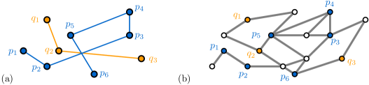
Figure 1: (a) $\mathcal{X}$ may be Euclidean space. (b) $\mathcal{X}$ may be a weighted graph under the shortest path metric. Observe that in full generality when $\mathcal{X}$ is a graph, any sequence of vertices may be a curve.

Discrete similarity measures between curves.

The Hausdorff distance can be defined between any two sets $P$ and $Q$. The discrete directed Hausdorff distance from $P$ to $Q$ is:

$${D_{\mathcal{H}}}(P\!\to\!Q):=\max_{p_{i}\in P}\min_{q_{j}\in Q}d(p_{i},q_{j}).$$

The discrete Hausdorff distance ${D_{\mathcal{H}}}(P,Q)$ is the maximum of ${D_{\mathcal{H}}}(P\!\to\!Q)$ and ${D_{\mathcal{H}}}(Q\!\to\!P)$. To define the discrete Fréchet distance we first define discrete walks: given two curves $P$ and $Q$ in $\mathcal{X}$, we denote by $[n]\times[m]$ the $n$ by $m$ integer lattice. We say that an ordered sequence $F$ of points in $[n]\times[m]$ is a discrete walk if for every consecutive pair $(i,j),(k,l)\in F$, we have $k\in\{i-1,i,i+1\}$ and $l\in\{j-1,j,j+1\}$. It is furthermore $xy$-monotone when we restrict to $k\in\{i,i+1\}$ and $l\in\{j,j+1\}$. Let $F$ be a discrete walk from $(1,1)$ to $(n,m)$. The cost of $F$ is the maximum over $(i,j)\in F$ of $d(p_{i},q_{j})$. The discrete Fréchet distance is the minimum over all $xy$-monotone walks $F$ from $(1,1)$ to $(n,m)$ of its associated cost:

$${D_{\mathcal{F}}}(P,Q):=\min_{F}\textnormal{cost}(F)=\min_{F}\max_{(i,j)\in F}d(p_{i},q_{j}).$$

The discrete weak Fréchet distance ${D^{w}_{\mathcal{F}}}$ is defined analogously, not requiring $F$ to be $xy$-monotone. Apart from lower bounds, all mentioned results for Fréchet distance will apply to the weak variant. In this paper we, given a $(1+\alpha)$-approximate distance oracle, also define what we call the perceived similarity between curves: ${D_{\mathcal{H}}}^{\circ}$, ${D_{\mathcal{F}}}^{\circ}$ and ${D^{w}_{\mathcal{F}}}^{\circ}$. These similarity measures are defined analogously, where $d(p_{i},q_{j})$ is replaced by $d^{\circ}(p_{i},q_{j})$ in their definition.

Free space matrix (FSM).

The FSM for a fixed $\rho^{*}\geq 0$ is a $|P|\times|Q|$, $(0,1)$-matrix where the cell $(i,j)$ is zero if and only if the distance between the $i$’th point in $P$ and the $j$’th point in $Q$ is at most $\rho^{*}$. Per definition, ${D_{\mathcal{F}}}(P,Q)\leq\rho^{*}$ if and only if there exists a ($xy$-monotone) discrete walk $F$ from $(1,1)$ to $(n,m)$ where for all $(i,j)\in F$: the cell $(i,j)$ is zero.

Problem statement.

Our data structure input is a curve $P=(p_{1},p_{2},\ldots,p_{n})$. For a given similarity measure ${D_{\star}}$, we make a distinction between three types of (approximate) queries: decision queries receive as input a curve $Q=(q_{1},q_{2},\ldots,q_{m})$ in $\mathcal{X}$ and a real value $\rho$. We want to output a Boolean indicating whether ${D_{\star}}(P,Q)\leq\rho$. Value queries receive as input a curve $Q$ and want to output a value $c$ with $c={D_{\star}}(P,Q)$. Subcurve queries compute the similarity measure to a subcurve $P[i,j]$. The number of vertices $m$ of $Q$ is part of the query input and may vary. Formally, given a similarity measure ${D_{\star}}$, we preprocess $P$ subject to:

• A-decision$(Q,\varepsilon,\rho)$: for $\rho\geq 0$ and $0<\varepsilon<1$ outputs a Boolean concluding either ${D_{\star}}(P,Q)>\rho$, or ${D_{\star}}(P,Q)\leq(1+\varepsilon)\rho$ (these two options are not mutually exclusive).

• A-value$(Q,\varepsilon)$: for $0<\varepsilon<1$ outputs a value in $[(1-\varepsilon){D_{\star}}(P,Q),(1+\varepsilon){D_{\star}}(P,Q)]$.

• Subcurve($Q,\rho,\varepsilon,i,j$): considers a subcurve $P[i,j]$. We define two queries equivalent to the two above for similarity between the subcurve $P[i,j]$ and a query $Q$.

We want a solution that is efficient in time and space, where time and space is measured in units of $\varepsilon,n,m,\rho$ and the distance oracle query time $T_{\alpha}$.

Curve simplification.

To efficiently compute the approximate Fréchet distance between two curves, Driemel, Har-peled and Wenk [22] introduce the concept of $\mu$-simplified curves. For a parameter $\mu\in\mathbb{R}$ one can construct a curve $P^{\mu}$ as follows. Start with the initial vertex $p_{1}$, and set this as the current vertex $p_{i}$. Next, scan the polygonal curve to find the first vertex $p_{j}$ such that $d(p_{i},p_{j})>\mu$. Add $p_{j}$ to $P^{\mu}$, and set $p_{j}$ as the current vertex. Continue this process until we reach the end of the curve. Finally, add the last vertex $p_{n}$ to $P^{\mu}$. Driemel, Har-peled and Wenk [22] observe any $\mu$-simplified curve $P^{\mu}$ can be computed in linear time and ${D_{\mathcal{F}}}(P^{\mu},P)<\varepsilon$. This leads to the following approximate decision algorithm:

1. Given $P,\varepsilon,Q$ and $\rho$, construct $P^{\frac{\varepsilon\rho}{4}}$ and $Q^{\frac{\varepsilon\rho}{4}}$ in $O(n+m)$ time.

2. Denote by $Z$ the number of zeroes in the FSM between $P^{\frac{\varepsilon\rho}{4}}$ and $P^{\frac{\varepsilon\rho}{4}}$ for $\rho^{*}=(1+\varepsilon/2)\rho$.

3. Using DFS over the FSM, and $O(Z)$ distance computations, test if ${D_{\mathcal{F}}}(P^{\frac{\varepsilon\rho}{4}},Q^{\frac{\varepsilon\rho}{4}})\leq\rho^{*}$.

   • They prove that: if yes then ${D_{\mathcal{F}}}(P,Q)\leq(1+\varepsilon)\rho$. If no then ${D_{\mathcal{F}}}(P,Q)>\rho$.

   • They upper bound $Z$ by $O(\frac{c(n+m)}{\varepsilon})$.

In this paper, we show that it suffices to assume that only $P$ is $c$-packed and upper bound $Z$ by $O(\frac{cm}{\varepsilon})$ instead. We extend the analysis to work with approximate distance oracles, and show a data structure to execute step 3 in time independent of $|P|=n$.

Redefining $\mu$-simplifications.

To facilitate efficient computations, we redefine what a $\mu$-simplification is. We show that our new definition is equivalent, in the sense that it implies the same theoretical guarantees. Formally, we say that henceforth the $\mu$-simplification is obtained by starting with $p_{1}$, and recursively adding the first $p_{j}$ such that the length of the subtrajectory $\ell(P[i,j])>\mu$. This way, our definitions (and computations) of $\mu$-simplifications are independent of the ambient space and only depend on the edge lengths of $P$.

From decision variant to computing Fréchet distance.

Suppose that we are given an algorithm to compute A-decision$(Q,\varepsilon,\rho)$ in $O(T)$ time. Then this may be used to answer A-value$(Q,\varepsilon)$ in $O(T^{2})$ time through parametric search [33, 32], which is not so attractive. Driemel, Har-peled and Wenk [22] have a static algorithm for A-decision$(Q,\varepsilon,\rho)$ that takes $O(\frac{c(n+m)}{\varepsilon})$ distance computations. They perform an approximate binary search for the appropriate $\rho$ over events where either the simplification of the input curves change, or when the reachability in the free space matrix changes. For the continuous Fréchet distance, we have vertex-vertex events and vertex-edge events. We will focus on the vertex-vertex events as these are the only relevant events to the discrete Fréchet distance.

For vertex-vertex events, they begin by constructing a well-separated pair decomposition (WSPD) on $(P,Q)$. This takes $O(2^{d}n+dn\log n)$ time (assuming $n\geq m$) and partitions $(P,Q)$ into $O(2^{d}n)$ pairs $(P_{i},Q_{i})$. For each pair $P_{i}\subseteq P,Q_{i}\subset Q$ there exists a value $c_{i}$ with $c_{i}<d(p,q)<2\cdot c_{i}$ for all $(p,q)\in P_{i}\times Q_{i}$. This provides a set of $O(2^{d}n)$ candidate choices for $\rho$. Naïvely, binary searching over these values takes $O(T\cdot\log(2^{d}n))$ time. Some further observations reduce their running time to $O(d\cdot n\cdot\left(\frac{c}{\varepsilon}+2^{d}+c\log n)\right))$ total time (assuming distance computation takes $O(d)$ time and $n\geq m$). Bringmann and Künnemann go from the decision variant to computations using [22]. Hence, their running time implicitly becomes $O(2^{d}n+d\cdot\frac{cn}{\sqrt{\varepsilon}}+d\cdot cn\log(2^{d}n))$. Using a WSPD has three downsides:

1. It is only known how to compute a WSPD for doubling metrics [49].

2. For non-constant dimensions $d$, computing a WSPD dominates the running time.

3. Computing a WSPD between $P$ and $Q$ takes $\Omega(|P|)$ time: which is undesirable for queries.

Due to downside 1, Driemel, van der Hoog and Rotenberg [22] approximate the discrete Fréchet distance in a graph through binary search over the sorted edges of $G$. This, at query time, takes time proportional to the size of $G$, whose size may exceed $n$ and $m$. We show that, through clever analysis, it suffices to map $P$ to points $P^{\prime}\subset\mathbb{R}^{1}$ (where points $p_{i}$ get mapped to the length $\ell(P[1,i])$). We then compute a WSPD of $P^{\prime}\times P^{\prime}$ in $O(n\log n)$ time, regardless of the ambient space $\mathcal{X}$. This not only allows us to approximate ${D_{\mathcal{F}}}(P,Q)$ independent of $n$, and the complexity of $\mathcal{X}$. It also allows us to approximate ${D_{\mathcal{F}}}(P,Q)$ in spaces for which no WSPD-analogue yet exists (e.g., polygonal domains under the geodesic distance).

Results.

In Section 3, we study computing the discrete Fréchet distance in a data structure setting. Just as for previous works, our results also apply to the weak Fréchet distance.

Theorem 2.1.

Let $\mathcal{X}$ be a metric space and $\mathcal{D}_{\mathcal{X}}^{\alpha}$ be a $(1+\alpha)$-approximate distance oracle with $O(T_{\alpha})$ query time. Let $P=(p_{1},\ldots,p_{n})$ be any $c$-packed curve in $\mathcal{X}$. We can store $P$ using $O(n)$ space and preprocessing, such that for any curve $Q=(q_{1},\ldots,q_{m})$ in $\mathcal{X}$ and any $\rho>0$ and $0<\varepsilon<1$, we can answer A-decision$(Q,\varepsilon,\rho)$ for the discrete Fréchet distance in:

$$O\left(\frac{c\cdot m}{\varepsilon}\cdot\left(T_{\varepsilon/6}+\log n\right)\right)\textnormal{ time.}$$

Corollary 2.2.

Using Oracles 1, it follows for a $c$-packed $P$ and the Fréchet distance that:

• For $\mathcal{X}=\mathbb{R}^{d}$ under $L_{1},L_{2},L_{\infty}$ metric in the real-RAM model, we can store $P$ using $O(n)$ space and preprocessing, to answer A-decision$(Q,\varepsilon,\rho)$ in $O\left(\frac{cm}{\varepsilon}\cdot\left(d+\log n\right)\right)$ time.

  • Improving the static $O(d\cdot\frac{cn}{\sqrt{\varepsilon}}+d\cdot cn\log n)$ algorithm by Bringmann and Künnemann [8, IJCGA’17]: making it faster when $n>m$ and making it a data structure.

• For $\mathcal{X}=\mathbb{R}^{d}$ under $L_{2}$ in word-RAM, we can store $P$ using $O(n)$ space and preprocessing, to answer A-decision$(Q,\varepsilon,\rho)$ in $O\left(\frac{cm}{\varepsilon}\cdot\left(d\log\varepsilon^{-1}+\log n\right)\right)$ worst case time.

  • Improving the static expected $O(d^{2}\cdot\frac{cn}{\sqrt{\varepsilon}}+d^{2}\cdot cn\log n)$ algorithm by Bringmann and Künnemann [8, IJCGA’17]: saving a factor $d$ and obtaining deterministic guarantees.

• For $\mathcal{X}$ a planar graph under the shortest path metric, we can store $P$ using $O(N^{1+o(1)})$ space and preprocessing, to answer A-decision$(Q,\varepsilon,\rho)$ in $O\left(\frac{cm}{\varepsilon}\cdot\log^{2+o(1)}N\right)$ time.

  • Generalizing the static $O\left(N^{1+o(1)}+\frac{c\cdot m}{\varepsilon}\log^{2+o(1)}N\right)$ algorithm by Driemel, van der Hoog and Rotenberg [25, SoCG’22] to a data structure.

• For $\mathcal{X}$ a graph under the shortest path metric, we can fix $\varepsilon$ and store $P$ using $O(\frac{N}{\varepsilon}\log N)$ space and preprocessing, to answer A-decision$(Q,\varepsilon,\rho)$ in $O\left(\frac{cm}{\varepsilon}\cdot(\varepsilon^{-1}+\log n)\right)$ time.

  • Generalizing the static $O\left(N^{1+o(1)}+\frac{c\cdot m}{\varepsilon}\log^{2+o(1)}N\right)$ algorithm by Driemel, van der Hoog and Rotenberg [25, SoCG’22] to a data structure.

We also use Theorem 2.1 to answer value queries. To this end, we develop a new technique that circumvents computing a WSPD between $P$ and $Q$ in $\mathcal{X}$ as we obtain the following:

Theorem 2.3.

Let $\mathcal{X}$ be a metric space and $\mathcal{D}_{\mathcal{X}}^{\alpha}$ be a $(1+\alpha)$-approximate distance with $O(T_{\alpha})$ query time. Let $P=(p_{1},\ldots,p_{n})$ be any $c$-packed curve in $\mathcal{X}$. We can store $P$ using $O(n)$ space and $O(n\log n)$ preprocessing time, such that for any curve $Q=(q_{1},\ldots,q_{m})$ in $\mathcal{X}$ and any $0<\varepsilon<1$, we can answer A-Value$(Q,\varepsilon)$ for the discrete Fréchet distance in:

$$O\left(\frac{c\cdot m}{\varepsilon}\cdot\log n\cdot\left(T_{\varepsilon/6}+\log\frac{c\cdot m}{\varepsilon}+\log n\right)\right)\textnormal{ time}.$$

Corollary 2.4.

Using Oracles 1. We have for $c$-packed $P$ and the discrete Fréchet distance:

• For $\mathcal{X}=\mathbb{R}^{d}$ in the real-RAM model, we can store $P$ using $O(n)$ space and $O(n\log n)$ preprocessing, to answer A-value$(Q,\varepsilon)$ in $O\left(\frac{cm}{\varepsilon}\log n(d+\log\frac{c\cdot m}{\varepsilon}+\log n\right)$ time.

  • Improving the static $O(2^{d}n+d\cdot\frac{cn}{\sqrt{\varepsilon}}+d^{2}\cdot cn\log n)$ algorithm Bringmann and Künnemann [8, IJCGA’17]: removing the exponential dependency on the dimension $d$.

  • Improving the dynamic $O(\left(O(\frac{1}{\varepsilon})\right)^{dm}\log\frac{1}{\varepsilon})$ space solution with $\tilde{O}(m\cdot d)$ query time by Filtser and Filtser [28, SODA’21]: allowing $Q$ to have arbitrary length, and using linear as opposed to exponential space and preprocessing time. This applies only when $P$ is $c$-packed, but is an improvement even for non-constant $c$.

• For $\mathcal{X}=\mathbb{R}^{d}$ under the $L_{2}$ metric in word-RAM, we can store $P$ using $O(n)$ space and preprocessing, to answer A-value$(Q,\varepsilon)$ in $O\left(\frac{cm}{\varepsilon}\log n(d\log n+\log\frac{c\cdot m}{\varepsilon}\right)$ time.

  • Improving upon the static expected $O(2^{d}n+d^{2}\cdot\frac{cn}{\sqrt{\varepsilon}}+d^{3}\cdot cn\log n)$ algorithm by Bringmann and Künnemann [8, IJCGA’17]: saving a factor $d2^{d}$ with deterministic guarantees.

• For $\mathcal{X}$ a planar graph under the SP metric, we can store $P$ using $O(N^{1+o(1)})$ space and preprocessing, to answer A-value$(Q,\varepsilon)$ in $O\left(\frac{c\cdot m}{\varepsilon}\log n\cdot(\log^{2+o(1)}N+\log\frac{c\cdot m}{\varepsilon})\right)$ time.

  • Improving the static $O\left(N^{1+o(1)}+|E|\log|E|+\frac{c\cdot m}{\varepsilon}\log^{2+o(1)}N\log|E|\right)$ algorithm by Driemel, van der Hoog and Rotenberg [25, SoCG’22]: making it a data structure and avoiding running time in $|E|$ given a distance oracle.

• For $\mathcal{X}$ a graph under the SP metric, we can fix $\varepsilon$ and store $P$ using $O(\frac{N}{\varepsilon}\log N)$ space and preprocessing, to answer A-value$(Q,\varepsilon)$ in $O\left(\frac{cm}{\varepsilon}\cdot\log n\cdot(\varepsilon^{-1}+\log\frac{c\cdot m}{\varepsilon}+\log n)\right)$ time.

  • Same improvement as above, except that this result is not adaptive to $\varepsilon$.

• For $\mathcal{X}$ a simple polygon under geodesics, we can store $P$ using $O(N\log N+n)$ space and preprocessing, to answer A-value$(Q,\varepsilon)$ in $O\left(\frac{cm}{\varepsilon}\cdot\log n\cdot(\log N+\log\frac{c\cdot m}{\varepsilon}+\log n)\right)$ time.

  • No realism-parameter algorithm was known in this setting, due to lack of WSPD.

We briefly note that all our results are also immediately applicable to subcurve queries:

Corollary 2.5.

All results obtained in Section 3 can answer the subcurve variants of the A-decision and A-value queries for any $i,j\in[n]$ at no additional cost.

Our data structure can be constructed, stored and queried with deterministic worst-case guarantees. We can update our data structure through a randomized algorithm:

Theorem 2.6.

We support updates to $P$, appending to or reducing the start or end of $P$, in $O(\log^{2}n)$ time (with high probability per update).

The appendix is dedicated to applying our techniques beyond the discrete Fréchet distance. In Appendix A we show that we can approximate the Hausdorff distance also. In Appendix B we show that your WSPD technique can be used to improve the query time from [32, SODA’23] from $O(m\log m\cdot(\log^{4}n+c^{4}\varepsilon^{-8}\log^{2}n))$ to $O(m(\log n+\log\varepsilon^{-1})\cdot(\log^{2}n+c^{2}\varepsilon^{-4}\log n))$.

3 Approximate Discrete Fréchet distance

In this section we simultaneously approximate the discrete weak Fréchet distance and the discrete Fréchet distance. For ease of exposition, we focus on the Fréchet distance, and indicate where algorithms are different for the weak Fréchet distance. We denote by $\mathcal{D}_{\mathcal{X}}^{\alpha}$ a $(1+\alpha)$-approximate distance oracle over our metric space $\mathcal{X}$. We receive as input some curve $P=(p_{1},\ldots,p_{n})$ in $\mathcal{X}$ which is $c$-packed in $\mathcal{X}$ for some $c\geq 1$. The goal is to preprocess $P$ to:

• answer A-decision$(Q,\varepsilon,\rho)$ for any curve $Q=(q_{1},\ldots,q_{m})$, $\rho>0$ and $0<\varepsilon<1$,

• answer A-value$(Q,\varepsilon)$ for any curve $Q=(q_{1},\ldots,q_{m})$ and $0<\varepsilon<1$.

We obtain this result in four steps. In Section 3.1 we define a $(0,1)$-matrix $M^{A\times Q}_{\rho^{*}}$ for any two curves $A$ and $Q$ and any $\rho^{*}>0$. We show that if $A$ is the $\mu$-simplified curve $P^{\mu}$ for some convenient $\mu$, then the number of zeroes in $M^{P^{\mu}\times Q}_{\rho^{*}}$ is bounded. In Section 3.2, we show that we can answer A-decision$(Q,\varepsilon,\rho)$ through inspecting all the zeroes the matrix $M^{P^{\mu}\times Q}_{\rho^{*}}$ for some convenient choice of $\mu$ and $\rho^{*}$. In Section 3.3, we show a data structure that stores $P$ to answer A-decision$(Q,\varepsilon,\rho)$. We show how to cleverly navigate $M^{P^{\mu}\times Q}_{\rho^{*}}$ for conveniently chosen $\mu$ and $\rho^{*}$. The key insight in this new technique, is that we may steadily increase $\rho^{*}$ whilst navigating the matrix. Finally, we extend this solution to answer A-value$(Q,\varepsilon)$.

3.1 Perceived free space matrix and free space complexity

We define the perceived free space matrix to help answer A-decision queries. Given two curves $(A,Q)$ and some $\rho$, we construct an $|A|\times|Q|$ matrix which we call the perceived free space matrix $M^{A\times Q}_{\rho}$. The $i$’th column corresponds to the $i$’th element $A[i]$ in $A$. We assign to each matrix cell $M^{P\times Q}_{\rho}[i,j]$ the integer $0$ if $d^{\circ}(A[i],q_{j})\leq\rho$ and integer $1$ otherwise.

For all $0<\varepsilon<1$, $\rho^{*}\geq 0$, and curves $A$ and $Q$, the discrete Fréchet distance between $A$ and $Q$ is at most $\rho^{*}$ if and only if there exists an ($xy$-monotone) discrete walk $F$ from $(1,1)$ to $(|A|,|Q|)$ where $\forall(i,j)\in F$, $M^{A\times Q}_{\rho^{*}}[i,j]=0$.

Computing ${D_{\mathcal{F}}}^{\circ}(P^{\mu},Q)$.

Previous results for approximating the Fréchet distance upper bound for any choice of $\rho$, the number of zeroes in the FSM between $P^{\varepsilon\rho}$ and $Q^{\varepsilon\rho}$. We show something stronger: we consider the perceived FSM instead, and introduce a new parameter $k\geq 1$ (which we leverage to be enable approximate distance oracles). For any value $\rho$ and some simplification value $\mu\geq\frac{\varepsilon\rho}{k}$, we subsequently upper bound the number of zeroes in the perceived FSM $M^{P^{\mu}\times Q}_{\rho^{*}}$ for the conveniently chosen $\rho^{*}=(1+\frac{\varepsilon}{2})\rho$:

Lemma 3.1.

Let $P=(p_{1},\ldots,p_{n})$ be a $c$-packed curve in $\mathcal{X}$. For any $\rho>0$ and $0<\varepsilon<1$, denote $\rho^{*}=(1+\frac{\varepsilon}{2})\rho$. For any $k\geq 1$, denote by $P^{\mu}$ its $\mu$-simplified curve for $\mu\geq\frac{\varepsilon\rho}{k}$. For any curve $Q=(q_{1},\ldots,q_{m})\subset\mathcal{X}$ the matrix $M^{P^{\mu}\times Q}_{\rho^{*}}$ contains at most $8\cdot\frac{c\cdot k}{\varepsilon}$ zeroes per row.

Proof 3.2.

The proof is by contradiction. Suppose that the $j$’th row of $M^{P^{\mu}\times Q}_{\rho^{*}}$ contains strictly more than $8\cdot\frac{c\cdot k}{\varepsilon}$ zeroes. Let $P_{0}\subset P^{\mu}$ be the vertices corresponding to these zeroes. Consider the ball $B_{1}$ centered at $q_{j}$ with radius $|B_{1}|=(1+\alpha)\rho^{*}$ and the ball $B_{2}$ with radius $2|B_{1}|$ (Figure 2). Each $p_{i}\in P_{0}$ must be contained in $B_{1}$ (indeed, the distance from $p_{i}$ to $q_{j}$ along $P$ is at most $(1+\alpha)\rho^{*}$ and thus: $d(p_{i},q_{j})\leq(1+\alpha)\rho^{*})$. For each $p_{i}\in P_{0}$ denote by $S_{i}$ the segment of $P$ starting at $p_{i}$ of length $\mu$. Observe that since $\varepsilon<1$: $S_{i}\subset B_{2}$. Per definition of simplification, each $S_{i}$ are each non-coinciding subcurves. This lower bounds $\ell(P\cap B_{2})$:

$$\ell(P\cap B_{2})\geq\sum_{p\in P_{0}}\ell(S_{i})=\sum_{p\in P_{0}}\mu>2(1+\alpha)(1+\frac{\varepsilon}{2})\cdot\frac{c\cdot k}{\varepsilon}\cdot\mu\geq 2(1+\alpha)\cdot c\cdot\rho^{*}\geq c\cdot|B_{2}|.$$

This contradicts the assumption that $P$ was $c$-packed.

Corollary 3.3.

Let $P=(p_{1},\ldots,p_{n})$ be a $c$-packed curve in $\mathcal{X}$. For any $\rho>0$ and $0<\varepsilon<1$, denote $\rho^{*}=(1+\frac{\varepsilon}{2})\rho$. For any $k\geq 1$, denote by $P^{\mu}$ its $\mu$-simplified curve for $\mu\geq\frac{\varepsilon\rho}{k}$. For any curve $Q=(q_{1},\ldots,q_{m})\subset\mathcal{X}$ the matrix $M^{P^{\mu}\times Q}_{\rho^{*}}$ contains at most $8\cdot\frac{c\cdot k}{\varepsilon}\cdot m$ zeroes.

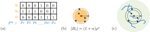
Figure 2: (a) For some value of $\mu$, the $\mu$-simplified curve is $(p_{1},p_{5},p_{6},\ldots,p_{27},p_{n})$. We show the matrix $M^{P^{\mu}\times Q}_{\rho^{*}}$. (b) For the point $q_{3}$, we claim that there are more than $Z=8\frac{ck}{\varepsilon}$ zeroes in its corresponding row. Thus, the ball $B_{1}$ with radius $(1+\alpha)\rho^{*}$ contains more than $Z$ points. (c) For each of these points, there is a unique segment along $P$ contained in the ball $B_{2}$.

3.2 Perceived distance implies distance

We show that we can use ${D_{\mathcal{F}}}^{\circ}(P^{\mu},Q)$ for some $\mu$-simplification to answer A-decision$(Q,\rho,\varepsilon)$:

Lemma 3.4.

For any $\rho>0$ and $0<\varepsilon<1$, choose $\rho^{*}=(1+\frac{1}{2}\varepsilon)\rho$ and $\mu\leq\frac{1}{6}\varepsilon\rho$. Let $\mathcal{X}$ be a metric space and $\mathcal{D}_{\mathcal{X}}^{\varepsilon/6}$ be a $(1+\frac{1}{6}\varepsilon)$-approximate distance oracle. For a $c$-packed curve $P=(p_{1},\ldots,p_{n})$ in $\mathcal{X}$ and any curve $Q=(q_{1},\ldots,q_{m})$ in $\mathcal{X}$:

• If ${D_{\mathcal{F}}}^{\circ}(P^{\mu},Q)\leq\rho^{*}$ then ${D_{\mathcal{F}}}(P,Q)\leq(1+\varepsilon)\rho$.

• If ${D_{\mathcal{F}}}^{\circ}(P^{\mu},Q)>\rho^{*}$ then ${D_{\mathcal{F}}}(P,Q)>\rho$.

Proof 3.5.

Per definition of $\mathcal{D}_{\mathcal{X}}^{\varepsilon/6}$: $\forall(p,q)\in P\times Q$, $d^{\circ}(p,q)\in[(1-\frac{1}{6}\varepsilon)d(p,q),(1+\frac{1}{6}\varepsilon)d(p,q)]$.

It follows from $0<\varepsilon<1$ that:

$$\forall(p,q)\in P\times Q:\quad d(p,q)\leq\left(1+\frac{1.1}{6}\varepsilon\right)d^{\circ}(p,q)\quad\wedge\quad d^{\circ}(p,q)\leq\left(1+\frac{1}{6}\varepsilon\right)d(p,q).$$

Suppose that ${D_{\mathcal{F}}}^{\circ}(P^{\mu},Q)\leq\rho^{*}$. There exists a (monotone) discrete walk $F$ through $P^{\mu}\times Q$ such that for each $(i,j)\in F$: $d^{\circ}(P^{\mu}[i],q_{j})\leq\rho^{*}=(1+\frac{1}{2}\varepsilon)\rho$. It follows that:

$$d(P^{\mu}[i],q_{j})\leq\left(1+\frac{1.1}{6}\varepsilon\right)d^{\circ}(P^{\mu}[i],q_{j})\leq\left(1+\frac{1.1}{6}\varepsilon\right)\left(1+\frac{1}{2}\varepsilon\right)\rho\leq\left(1+\frac{5}{6}\varepsilon\right)\rho.$$

We will prove that this implies ${D_{\mathcal{F}}}(P,Q)\leq(1+\varepsilon)\rho$. We use $F$ to construct a discrete walk $F^{\prime}$ through $P\times Q$. For each consecutive pair $(a,b),(c,d)\in F$ note that since $F$ is a discrete walk, $P^{\mu}[a]$ and $P^{\mu}[c]$ are either the same vertex or incident vertices on $P^{\mu}$. Denote by $P_{ac}$ the vertices of $P$ in between $P^{\mu}[a]$ and $P^{\mu}[c]$. It follows that:

$$\forall p^{\prime}\in P_{ac}:\quad d(p^{\prime},q_{b})\leq d\left(P^{\mu}[a],q_{b}\right)+\mu\leq(1+\frac{5}{6}\varepsilon)\rho+\frac{1}{6}\varepsilon\rho=(1+\varepsilon)\rho.$$

Now consider the following sequence of pairs of points:

$L_{ac}=(P^{\mu}[a],q_{b})\cup\{(p^{\prime},q_{b})\mid p^{\prime}\in P_{ac}\}\cup(P^{\mu}[c],q_{d}).$ We add the lattice points corresponding to $L_{ac}$ to $F^{\prime}$. It follows that we create a discrete walk $F^{\prime}$ in the lattice $|P|\times|Q|$ where for each $(i,j)\in F^{\prime}$: $d(p_{i},q_{j})\leq(1+\varepsilon)\rho$. Thus, ${D_{\mathcal{F}}}(P,Q)\leq(1+\varepsilon)\rho$.

Suppose otherwise that ${D_{\mathcal{F}}}(P,Q)\leq\rho$. We will prove that ${D_{\mathcal{F}}}^{\circ}(P^{\mu},Q)\leq\rho^{*}$. Indeed, consider a discrete walk $F^{\prime}$ in the lattice $|P|\times|Q|$ where for each $(i,j)\in F^{\prime}$: $d(p_{i},q_{j})\leq\rho$. We construct a discrete walk $F$ in $|P^{\mu}|\times|Q|$. Consider each $(i,j)\in F^{\prime}$, If $p_{i}=P^{\mu}[a]$ for some integer $a$, we add $(a,j)$ to $F$. Otherwise, denote by $P^{\mu}[a]$ the last vertex on $P^{\mu}$ that precedes $p_{i}$: we add $(a,j)$ to $F$. Note that per definition of $\mu$-simplification, $d(P^{\mu}[a],q_{j})\leq d(p_{i},q_{j})+\mu\leq(1+\frac{1}{6}\varepsilon)\rho$. It follows from the definition of our approximate distance oracle that $d^{\circ}(P^{\mu}[a],q_{j})\leq(1+\frac{1}{6}\varepsilon)(1+\frac{1}{6}\varepsilon)\rho<(1+\frac{1}{2}\varepsilon)\rho=\rho^{*}$. Thus, we may conclude that ${D_{\mathcal{F}}}^{\circ}(P^{\mu},Q)\leq\rho^{*}$.

3.3 Answering A-decision$(Q,\varepsilon,\rho)$

We showed in Sections 3.1 and 3.2 that for any $c$-packed curve $P$, $\rho>0$ and $0<\varepsilon<1$ we can choose suitable values $\frac{\varepsilon\rho}{k}\leq\mu\leq\frac{\varepsilon\rho}{6}$. This upper bounds the number of zeroes in $M^{P^{\mu}\times Q}_{\rho^{*}}$. Moreover, for $\rho^{*}=(1+\frac{1}{\varepsilon})\rho$ we know that computing ${D_{\mathcal{F}}}^{\circ}(P^{\mu},Q)$ implies an answer to A-decision$(Q,\varepsilon,\rho)$. We now construct a data structure over $P$ such that for any value $\mu$, we can efficiently obtain $P^{\mu}$ and answer A-decision$(Q,\varepsilon,\rho)$. Note that we assume that the preprocessing input specifies the distance between consecutive points on $P$. This assumption may be lifted by incorporating the distance oracle query time into the preprocessing time.

Recall that we redefined the term $\mu$-simplification. This new definition allows for an efficient data structure, whose query time is independent of the ambient space $\mathcal{X}$:

Lemma 3.6.

Let $P=(p_{1},\ldots,p_{n})$ be a curve in $\mathcal{X}$. We can store $P$ using $O(n)$ space and preprocessing time, such that for any value $\mu\geq 0$ and any integer $N$ we can report the first $N$ vertices on the $\mu$-simplification $P^{\mu}$ in $O(N\log n)$ time.

Proof 3.7.

For each $1<i\leq n$ we create a half-open interval $(\ell(P[1,i-1]),\ell(P[1,i])]$ in $\mathbb{R}^{1}$. Each point in $P$ receives a pointer to its unique interval. This results in an ordered set of $O(n)$ disjoint intervals on which we build a balanced binary tree in $O(n)$ time.

For any given value $\mu$, we can now obtain the first $N$ vertices of $P^{\mu}$ as follows: First, we add $p_{1}$. Then, we inductively add subsequent vertices. Suppose that we just added $p_{i}$ to our output. We choose the value $a=\ell(P[1,i])+\mu$. we binary search in $O(\log n)$ time for the point $p_{j}$ where the interval $(\ell(P[1,j-1]),\ell(P[1,j])]$ contains $a$. Per definition of the intervals: the length $\ell(P[i,j])\geq\mu$. Moreover, for all $x\in(i,j)$ the length $\ell(P[i,x])<x$. Thus, $p_{j}$ is the successor of $p_{i}$ and we recurse if necessary.

Note that Lemma 3.6 can for any $\mu$ also report the $\mu$-simplification of $P[i,j]$ for any $(i,j)$ at query time. Therefore, Theorem 2.1 also immediately works for the subcurves query variants. We show that we can use our $\mu$-simplification to answer the decision variant:

See 2.1

Proof 3.8.

We store $P$ in the data structure of Lemma 3.6 using $O(n)$ space and preprocessing time. Given a query A-decision$(Q,\varepsilon,\rho)$ we choose $\alpha=\frac{1}{6}\varepsilon$, $\rho^{*}=(1+\frac{1}{2}\varepsilon)$ and $\mu=\frac{\varepsilon\rho}{6}$. We test if ${D_{\mathcal{F}}}^{\circ}(P^{\mu},Q)\leq\rho^{*}$. By Lemma 3.4, if ${D_{\mathcal{F}}}^{\circ}(P^{\mu},Q)\leq\rho^{*}$ then ${D_{\mathcal{F}}}(P,Q)\leq(1+\varepsilon)\rho$ and otherwise ${D_{\mathcal{F}}}(P,Q)>\rho$. We consider the matrix $M^{P^{\mu}\times Q}_{\rho^{*}}$.

By Observation 3.1, ${D_{\mathcal{F}}}^{\circ}(P^{\mu},Q)\leq\rho^{*}$ if and only if there exists a discrete walk $F$ from $(1,1)$ to $(|P^{\mu}|,|Q|)$ where for each $(i,j)\in F$: $M^{P^{\mu}\times Q}_{\rho^{*}}[i,j]=0$. We will traverse this matrix in a depth-first manner as follows: starting from the cell $(1,1)$, we test if $M^{P^{\mu}\times Q}_{\rho^{*}}[1,1]=0$. If so, we push $(1,1)$ onto a stack. Each time we pop a tuple $(i,j)$ from the stack, we inspect their $O(1)$ neighbors $\{(i+1,j),(i,j+1),(i+1,j+1)\}$ (we inspect twice as many neighbors for the weak Fréchet distance). If $M^{P^{\mu}\times Q}_{\rho^{*}}[i^{\prime},j^{\prime}]=0$, we push $(i^{\prime},j^{\prime})$ onto our stack. It takes $O(\log n)$ time to obtain the $i+1$’th vertex of $P^{\mu}$, and $O(T_{\varepsilon/6})$ to determine the value of e.g., $M^{P^{\mu}\times Q}_{\rho^{*}}[i+1,j]$. Thus each time we pop the stack, we spend $O(T_{\varepsilon/6})+\log n)$ time.

By Corollary 3.3 (noting $\varepsilon<1$ and setting $k=6$), we push at most $O(\frac{cm}{\varepsilon})$ tuples onto our stack. Therefore, we spend $O(\frac{cm}{\varepsilon}(T_{\varepsilon/6}+\log n))$ total time. By Observation 3.1, ${D_{\mathcal{F}}}^{\circ}(P^{\mu},Q)\leq\rho^{*}$ if and only if we push $(|P^{\mu}|,|Q|)$ onto our stack. We test this in $O(1)$ additional time per operation. Thus, the theorem follows.

3.4 Answering A-value$(Q,\varepsilon)$

Finally, we show how to answer the A-value$(Q,\varepsilon,\rho)$ query. Recall that previous methods to approximate the value ${D_{\mathcal{F}}}(P,Q)$ rely upon inefficient data structures: when $\mathcal{X}=\mathbb{R}^{d}$ a $d$-dimensional WSPD of $P\times Q$, and when $\mathcal{X}$ is a graph the sorted set of edges $E$. We circumvent this, by leveraging the variable $k\geq 1$ introduced in the definition of $\mu\geq\frac{\varepsilon\rho}{k}$:

See 2.3

Proof 3.9.

We preprocess $P$ using Lemma 3.6 in $O(n)$ space and time. We map $P$ onto $\mathbb{R}^{1}$ as follows: each vertex $p_{i}$ gets mapped to the value $\lambda_{i}=\ell(P[1,i])$. Denote by $\Lambda=\{\lambda_{i}\}$. As a second data structure, we compute a 1-dimensional WSPD on $\Lambda$ and itself in $O(n\log n)$ time using $O(n)$ space [35]. We obtain a partition of $P\times P$ into $O(n)$ sets $(P_{s},P_{s}^{\prime})$ where for each $s$, there exists a $c_{s}\in\mathbb{R}$ such that for all $p_{i}\in P_{s}$ and $p_{j}\in P_{s}^{\prime}$: $\ell(P[i,j])\in[c_{s},2\cdot c_{s}]$. We denote by $I_{s}=[c_{s},2\cdot c_{s}]$ the corresponding interval and obtain a sorted set of intervals $\mathcal{I}$.

Given a query $(Q,\varepsilon)$, we set $\alpha\leftarrow\varepsilon/6$ and obtain $\mathcal{D}_{\mathcal{X}}^{\alpha}$. We (implicitly) rescale each interval $I_{i}\in\mathcal{I}$ by a factor $\frac{6}{\varepsilon}$, creating for $I_{s}$ the interval $I_{s}^{\varepsilon}=[\frac{6\cdot c_{s}}{\varepsilon},\frac{12\cdot c_{s}}{\varepsilon}]$. This creates a sorted set $\mathcal{I}^{\varepsilon}$ of pairwise disjoint intervals. Intuitively, these are the intervals over $\mathbb{R}^{1}$ where for $\rho\in I_{s}^{\varepsilon}$, the $\mu$-simplification $P^{\mu}$ for $\mu=\frac{\varepsilon\rho}{6}$ may change.

We binary search over $\mathcal{I}^{\varepsilon}$. For each boundary point $\lambda$ of an interval $I_{s}^{\varepsilon}$ we query A-decision$(Q,\varepsilon,\lambda)$: discarding half of the remaining intervals in $\mathcal{I}^{\varepsilon}$. It follows that in $O(\frac{c\cdot m}{\varepsilon}\cdot\log n\cdot(T_{\varepsilon/6}+\log n))$ time, we obtain one of two things:

1. an interval $I_{s}^{\varepsilon}$ where $\exists\rho^{*}\in I_{s}^{\varepsilon}$ that is a $(1+\varepsilon)$-approximation of ${D_{\mathcal{F}}}(P,Q)$, or

2. a maximal interval $I^{*}$ disjoint of the intervals in $\mathcal{I}^{\varepsilon}$ where $\exists\rho^{*}\in I^{*}$ that is a $(1+\varepsilon)$-approximation of ${D_{\mathcal{F}}}(P,Q)$.

Denote by $\lambda$ the left boundary of $I_{s}^{\varepsilon}$ or $I^{*}$: it lower bounds ${D_{\mathcal{F}}}(P,Q)$. Note that if $I^{*}$ precedes all of $\mathcal{I}^{\varepsilon}$, $\lambda=0$. We now compute a $(1+\varepsilon)$-approximation of ${D_{\mathcal{F}}}(P,Q)$ as follows:

FindApproximation$(\lambda)$:

1. Compute $C=\frac{d^{\circ}(p_{1},q_{1})}{(1+\frac{1}{2}\varepsilon)}$.

2. Initialize $\rho^{*}\leftarrow(1+\frac{1}{2}\varepsilon)\cdot\max\{C,\lambda\}$ and set a constant $\mu\leftarrow\frac{\varepsilon}{6}\cdot\lambda$.

3. Push the lattice point $(1,1)$ onto a stack.

4. Whilst the stack is not empty do:

   • Pop a point $(i,j)$ and consider the $O(1)$ neighbors $(p_{a},q_{b})$ of $(p_{i},q_{j})$ in $M^{P^{\mu}\times Q}_{\rho^{*}}$:

     • If $d^{\circ}(p_{a},q_{b})\leq\rho^{*}$, push $(a,b)$ onto the stack.

     • Else, store $d^{\circ}(p_{a},q_{b})$ in a min-heap.

   • If we push $(p_{n},q_{m})$ onto the stack do:

     • Output $\nu=\frac{\rho^{*}}{(1+\frac{1}{2}\varepsilon)}$.

5. If the stack is empty, we extract the minimal $d^{\circ}(p_{a},p_{b})$ from the min-heap.

   • Update $\rho^{*}\leftarrow(1+\frac{1}{2}\varepsilon)\cdot d^{\circ}(p_{a},q_{b})$, push $(a,b)$ onto the stack and go to line 4.

Correctness.

Suppose that our algorithm pushes $(p_{n},q_{m})$ onto the stack and let at this time of the algorithm, $\rho^{*}=(1+\frac{1}{2}\varepsilon)\nu$. Per definition of the algorithm, $\nu\geq\lambda$ is the minimal value for which the matrix $M^{P^{\mu}\times Q}_{\rho^{*}}$ contains a walk $F$ from $(1,1)$ to $(n,m)$ where for each $(i,j)\in F$: $M^{P^{\mu}\times Q}_{\rho^{*}}[i,j]=0$. Indeed, each time we increment $\rho^{*}$ by the minimal value required to extend any walk in $M^{P^{\mu}\times Q}_{\rho^{*}}$. Moreover, we fixed $\mu\leftarrow\frac{\varepsilon}{6}\lambda$ and thus $\mu\leq\frac{\varepsilon}{6}\nu$. Thus we may apply Lemma 3.4 to defer that $\nu$ is the minimal value for which ${D_{\mathcal{F}}}(P,Q)\leq(1+\varepsilon)\nu$.

Running time.

We established that the binary search over $\mathcal{I}^{\varepsilon}$ took $O(\frac{c\cdot m}{\varepsilon}\cdot\log n\cdot(T_{\varepsilon/6}+\log n))$ time. We upper bound the running time of our final routine. For each pair $(p_{i},q_{j})$ that we push onto the stack we spend at most $O(T_{\varepsilon/6}+\log\frac{c\cdot m}{\varepsilon}+\log n)$ time as we:

• Obtain the $O(1)$ neighbors of $(p_{i},q_{j})$ through our data structure in $O(\log n)$ time,

• Perform $O(1)$ distance oracle queries in $O(T_{\varepsilon/6})$ time, and

• Possibly insert $O(1)$ neighbors into a min-heap. The min-heap has size at most $K$: the number of elements we push onto the stack. Thus, this takes $O(\log K)$ insertion time.

What remains is to upper bound the number of items we push onto the stack. Note that we only push an element onto the stack, if for the current value $\rho^{*}$ the matrix $M^{P^{\mu}\times Q}_{\rho^{*}}$ contains a zero in the corresponding cell. We now refer to our earlier case distinction.

Case (a): Since $\varepsilon<1$ we know that $\rho^{*}\in[\lambda,4\cdot\lambda]$. We set $\mu=\frac{\varepsilon}{6}\lambda$. So $\mu\geq\frac{1}{k}\varepsilon\rho^{*}$ for $k=24$. Thus, we may immediately apply Corollary 3.3 to conclude that we push at most $O(\frac{c\cdot m}{\varepsilon})$ elements onto the stack.

Case (b): Denote by $\gamma=\frac{\varepsilon}{6}\nu$. Per definition of our re-scaled intervals, the half-open interval $(\mu,\gamma]$ does not intersect with any interval in the non-scaled set $\mathcal{I}$. It follows that $P^{\mu}=P^{\gamma}$ and that for two consecutive vertices $p_{i},p_{l}\in P^{\mu}$: $\ell(P[i,l])>\gamma$. From here, we essentially redo Lemma 3.1 for this highly specialized setting. The proof is by contradiction, where we assume that for $\rho^{*}=(1+\frac{\varepsilon}{2})\nu$ there are more than $8\cdot 6\cdot\frac{c}{\varepsilon}$ in the $j$’th row of $M^{P^{\mu}\times Q}_{\rho^{*}}$. Denote by $P_{0}\subset P^{\mu}$ the vertices corresponding to these zeroes. We construct a ball $B_{1}$ centered at $q_{j}$ with radius $2\rho^{*}$ and a ball $B_{2}$ with radius $2|B_{1}|$. We construct a subcurve $S_{i}$ of $P$ starting at $p_{i}\in P_{0}$ of length $\gamma$. The critical observation is, that our above analysis implies that all the subcurves $S_{i}$ do not coincide (since each of them start with a vertex in $P^{\mu}$). Since $\varepsilon<1$, each segment $S_{i}$ is contained in $B_{2}$. However, this implies that $B_{2}$ is not $c$-packed since: $\ell(P\cap B_{2})\geq\sum_{i}\ell(S_{i})=\sum_{i}\gamma>8\cdot 6\frac{c}{\varepsilon}\gamma\geq 4\cdot c\cdot\rho^{*}\geq 2\cdot c\cdot|B_{2}|$. Thus, we always push at most $O(\frac{c\cdot m}{\varepsilon})$ elements onto our stack and this implies our running time.

4 Dynamic updates and subcurve queries

Finally, we expand our techniques to include updates. Note that our data structure can be constructed, stored and queried with deterministic worst-case time and space. We augment this structure, to allow for updates where we may append a new vertex to $P$ (appending it to either the start or end of $P$), or reduce $P$ by one vertex (removing either the start or end vertex). We assume that after each update, the curve remains $c$-packed (i.e., we are given some value $c$ beforehand which may over-estimate the $c$-packedness of the curve, but never underestimate it). Alternatively, the query may include the updated value for $c$, in which case our approach is adaptive to $c$. For simplicity, we assume that the update supplies us with the exact distance between the vertices affected by the update. In full generality, our algorithm may query the (approximate) distance oracles for these distance values and work with perceived lengths. Our data structure requires three components: a $\mu$-simplification data structure, a WSPD, and an estimate $c^{\prime}$ of the $c$-packedness. By assumption, we have access to the latter. We update the former two:

The $\mu$-simplification data structure.

Our $\mu$-simplification data structure stores for every $i$, the half-open interval $(\ell(P[1,i-1]),\ell(P[1,i])]$ in a balanced binary tree. The key observation here is that our algorithm does not require us to store each interval explicitly. Instead, it suffices to compute the width of each interval in the leaves of the tree. In each interior node $\nu$ of the tree, we store the sum of the width of all the leaves in the subtree rooted at $\nu$.

Lemma 4.1 (Analogue to Lemma 3.6).

We can update our $\mu$-simplification data structure in $O(\log n)$ worst case time after any insertion and deletion in $P$. Afterwards, we can report the first $N$ vertices on the $\mu$-simplification $P^{\mu}$ in $O(N\log n)$ time.

Proof 4.2.

After an update, we identify the leaves affected by this update in $O(\log n)$ time. We compute the new leaves of our tree in $O(1)$ time. Having inserted them, we rebalance the tree. For any given value $\mu$, we now obtain the first $N$ vertices of $P^{\mu}$ as follows: first, we add the vertex $p_{1}$. Now we apply induction, where we assume that we have just inserted $p_{i}$, and have a pointer to the leaf corresponding to $p_{i}$. From the leaf of $p_{i}$, we walk upwards until we are about to reach a node $\nu$ where the value stored at $\nu$ exceeds $\mu$. From there, we walk downwards in symmetric fashion and identify the vertex $p_{j}$ succeeding $p_{i}$.

The WSPD.

Fischer and Har-Peled [31] study the following problem: given a point set $M$ in $\mathbb{R}^{d}$ and a constant $\varepsilon$, maintain an WSPD of $M\times M$. For ease of exposition, we cite their more general result for our case where we have a point set in $\mathbb{R}^{1}$:

Lemma 4.3 (Theorem 12+13 in [31]).

Let $L$ be a list of Well-separated pairs of $M\times M$ for an $n$-point set $M$ in $\mathbb{R}^{1}$. With high probability, in time $O(\log^{2}n)$, one can modify $L$ to yield $\hat{L}$: the list of well-separated pairs of $M\times M$ after an insertion or deletion in $M$.

Recall that we have a $WSPD$ of $P^{\prime}\times P^{\prime}$: where $P^{\prime}$ is every point $p_{i}\in P$ mapped to $\ell(P[1,i])$. Thus, inserting a point into $P$, may change $O(n)$ points in $P^{\prime}$. However, note that pairwise distances of $P^{\prime}$ are preserved under translation of $P^{\prime}$. We maintain a WSPD of $M\times M$ where $M$ originally is $P^{\prime}$. Suppose that we receive a new point $p_{0}$ at the head of $P$, which is at distance $e$ from $p_{1}$. We insert into $M$ a new value, which is the value corresponding to $p_{1}$, minus $e$, and update the $WSPD$ in $O(\log^{2}n)$ time with high probability. Reducing $P$ or appending/reducing $P$ at its tail can be accomplished in the same way. It follows we maintain a WSPD of $M$ which is a translated version of $P^{\prime}$. Thus, Lemma 4.1 and 4.3 imply Theorem 2.6.

Appendix A Hausdorff

This section is dedicated to showing that our approach also works to compute a $(1+\varepsilon)$-approximation of the Hausdorff distance ${D_{\mathcal{H}}}(P,Q)$. Perhaps surprisingly, computing the Hausdorff distance is somewhat more complicated than computing the Fréchet distance. The intuition behind this, is as follows. Because $P$ is $c$-packed, we can upper bound for any decision variable $\rho$ the number of zeroes in the free-space matrix. For the discrete Fréchet distance, we are interested in a connected walk through the matrix that only consists of zeroes, hence we can find such a walk using depth-first search. For the decision variant of the Hausdorff distance, we require instead that the free space matrix contains a zero in every row and in every column. Since this does not have the same structure as a connected path, we require more work and more time to verify this. To this end, we assume that in the preprocessing phase we may compute a Voronoi diagram in $O(f(n))$ time, and that the Voronoi diagram has $O(g(n))$ query time. In $\mathbb{R}^{d}$ under the $L_{1},L_{2},L_{\infty}$ metric, a Voronoi diagram on $n$ points can be computed in $f(n)=O(n\log n+n^{\lfloor d/2\rfloor})$ time: it subsequently has $g(n)=O(\log n)$ query time. In a graph under the shortest path metric a Voronoi diagram on $n$ points can be computed in $O(|G|\log|G|)$ time and it has $O(1)$ query time [25].

Before we go into the details, we make one brief remark: for ease of exposition, throughout this section, we assume that our distance oracle $\mathcal{D}_{\mathcal{X}}^{\alpha}$ is an exact distance oracle. The reasoning behind this is that we want to simplify our analysis to focus on illustrating the difference between computing the Hausdorff and Fréchet distance. Approximate distance oracles may be assumed by introducing $\rho^{*}=(1+\frac{\varepsilon}{2})\rho$ and $\mu=\frac{\varepsilon\rho}{6}$ in the exact way as in Section 3. Again our approach immediately also works for subcurve query variants.

Hausdorff matrix.

For values $\rho^{*}\geq 0$ and some $0<\varepsilon<1$ we choose $\mu=\varepsilon\rho^{*}$. We define $H^{P^{\mu}\times Q}_{\rho}$ as a $(0,1)$-matrix of dimensions $|P^{\mu}|$ by $|Q|$ where rows correspond to the ordered vertices in $Q$ and columns to the ordered vertices in $P^{\mu}$. Let $p_{i}\in P$ and $p_{s}$ be its predecessor in $P^{\mu}$. For any $q_{j}\in Q$, we set the cell corresponding to $(p_{i},q_{j})$ to zero if there exists a $p^{\prime}\in P[i,s]$ such that $d(p^{\prime},q_{j})\leq\rho^{*}$. Otherwise, we set the cell to one. This defines $H^{P^{\mu}\times Q}_{\rho^{*}}$.

Lemma A.1.

Let $\mathcal{X}$ be any metric space and $P=(p_{1},\ldots,p_{n})$ and $Q=(q_{1},\ldots,q_{m})$ be curves in $\mathcal{X}$. For any $\rho^{*}\geq 0$, any $0<\varepsilon<1$ and $\mu\leq\varepsilon\rho^{*}$ : If there exists a zero in each row and each column of $H^{P^{\mu}\times Q}_{\rho^{*}}$ then ${D_{\mathcal{H}}}(P,Q)\leq(1+\varepsilon)\rho^{*}$. Otherwise, $H^{P^{\mu}\times Q}_{\rho^{*}}$ ${D_{\mathcal{H}}}(P,Q)>\rho^{*}$.

Proof A.2.

Suppose that there exists a zero in each row and each column of $H^{P^{\mu}\times Q}_{\rho^{*}}$. Consider a column in $H^{P^{\mu}\times Q}_{\rho^{*}}$ corresponding to a vertex $p_{s}\in P^{\mu}$ and let its $j$’th row contain a zero. Then for $p_{s}$ and all $p^{\prime}$ in between $p_{s}$ and its successor: $d(p^{\prime},q_{j})\leq\rho^{*}+\mu\leq(1+\varepsilon)\rho^{*}$. Thus ${D_{\mathcal{H}}}(P\rightarrow Q)\leq(1+\varepsilon)\rho^{*}$. Similarly, consider the $j$’th row in $H^{P^{\mu}\times Q}_{\rho^{*}}$ and let it contain a zero in its column corresponding to $p_{j}$. Then $d(p_{i},q_{j})\leq(1+\varepsilon)\rho^{*}$ and thus ${D_{\mathcal{F}}}(Q\rightarrow P)\leq\rho^{*}$.

From this point on, we observe that the proof of Lemma 3.1 immediately applies to the matrix $H^{P^{\mu}\times Q}_{\rho^{*}}$ (indeed, for any zero in the $j$’th row we still obtain a point in the ball $B_{1}$ – where the point may be some $p^{\prime}$ succeeding $p_{i}$. The segment $S_{i}$ subsequently must be entirely contained in $B_{2}$ and so the proof follows). Thus, we conclude:

Corollary A.3.

Let $P=(p_{1},\ldots,p_{n})$ be a $c$-packed curve in $\mathcal{X}$. For any $\rho^{*}>0$ and any $k>1$, denote by $P^{\mu}$ its $\mu$-simplified curve for $\mu\geq\frac{\varepsilon\rho^{*}}{k}$. For any curve $Q=(q_{1},\ldots,q_{m})\subset\mathcal{X}$ the matrix $H^{P^{\mu}\times Q}_{\rho^{*}}$ contains at most $8\cdot\frac{c\cdot k}{\varepsilon}\cdot m$ zeroes.

A.1 Answering A-decision$(Q,\varepsilon,\rho^{*})$.

Theorem A.4.

Let $\mathcal{X}$ be a metric space and $P=(p_{1},\ldots,p_{n})$ be any $c$-packed curve in $\mathcal{X}$. Suppose that we can construct a Voronoi diagram on $P$ in $O(f(n))$ time using $O(s(n))$ space and that it has $O(g(n))$ query time. We can store $P$ using $O((n+s(n))\log n)$ space and $O((n+f(n))\log n)$ preprocessing time, such that for any curve $Q=(q_{1},\ldots,q_{m})$ in $\mathcal{X}$, any $\rho^{*}\geq 0$ and $0<\varepsilon<1$, we can answer A-Decision$(Q,\varepsilon,\rho)$ for the Hausdorff distance in:

$$O\left(\frac{c\cdot m}{\varepsilon}\cdot\log n\cdot g(n)\right)\textnormal{ time}.$$

Proof A.5.

At preprocessing, we construct the data structure of Lemma 3.6. In addition, we create a balanced binary decomposition of $P$ where we recursively split $P$ into two curves $P_{1}$ and $P_{2}$ with a roughly equal number of vertices. For each node in the balanced binary decomposition, we create a Voronoi diagram on the corresponding (sub)curve. This takes $O((n+f(n))\log n)$ total time and $O((n+s(n))\log n)$ total space.

At query time, we receive $Q$ and a value $\rho^{*}\geq 0$. We set $\mu=\varepsilon\rho^{*}$ and in $O(\frac{c\cdot m}{\varepsilon}\log n)$ time we compute the first $8\frac{c\cdot m}{\varepsilon}$ vertices of $P^{\mu}$.

If we discover that $P^{\mu}$ has more than $8\frac{c\cdot m}{\varepsilon}$ elements, we report that ${D_{\mathcal{H}}}(P,Q)>\rho$. Indeed: if ${D_{\mathcal{H}}}(P,Q)\leq\rho$ then each column in $H^{P^{\mu}\times Q}_{\rho^{*}}$ must contain a zero. Since there are at most $m$ rows, then by the pigeonhole principle ${D_{\mathcal{H}}}(P,Q)\leq\rho$ only if $P^{\mu}$ contains at most $8\frac{c\cdot m}{\varepsilon}$ vertices. We store $P^{\mu}$ in a balanced binary tree $T$ (ordered along $P^{\mu}$) in $O(|P^{\mu}|)=O(\frac{c\cdot m}{\varepsilon})$ time. We now iterate over each of the vertices in $Q$ and do the following subroutine:

Subroutine$(q_{j}\in Q,T)$:

We execute each subroutine one by one, passing $T$ along. We maintain a stack of pairs of indices.

If after all subroutines $T$ is not empty, we output ${D_{\mathcal{H}}}(P,Q)>\rho$.

Otherwise, we output ${D_{\mathcal{H}}}(P,Q)\leq(1+\varepsilon)\rho$.

1. Push the pair $(1,n)$ onto a stack.

2. Whilst the stack is not empty, do:

   • Set $(i,j)\leftarrow\textsc{pop}$ and obtain $P[i,j]$ as $O(\log n)$ roots in our hierarchical decomposition.

   • For each of the roots, query their Voronoi diagram with $q_{j}$ in $O(\log n\cdot V_{\varepsilon/6})$ total time.

   • Let $p^{\prime}\in P[i,j]$ be the vertex realising the minimal distance to $q_{j}$.

     • If $d(p^{\prime},q)>\rho$: continue the loop with the next stack item.

   • Otherwise, find its predecessor $p_{s}$ in $P^{\mu}$ in $O(\log n)$ time.

   • Set the cell corresponding to $(p_{s},q_{j})$ in $H^{P^{\mu}\times Q}_{\rho^{*}}$ to zero.

   • Remove $p_{s}$ from $T$ in $O(\log\frac{c\cdot m}{\varepsilon})=O(\log n)$ time.

   • Let $p_{l}$ be the successor of $p_{s}$ in $P^{\mu}$.

   • Push $(i,s)$ and $(l,j)$ onto the stack.

3. If only $(1,n)$ was ever pushed onto the stack, terminate and output ${D_{\mathcal{H}}}(P,Q)>\rho$

   (no further subroutines are required).

Runtime.

Each time we push two items onto the stack, the subroutine has found in the $j$’th row of $H^{P^{\mu}\times Q}_{\rho^{*}}$ a new cell that has a zero. Thus, the subroutine can push at most $O(\frac{c}{\varepsilon})$ items on the stack. Per item on the stack, we take $O(\log n\cdot g(n))$ time. Thus, our algorithm takes $O(\frac{c\cdot m}{\varepsilon}\cdot\log n\cdot g(n))$ total time.

Correctness.

Finally, we show that our algorithm always outputs a correct conclusion through a case distinction on when we output an answer.

Let us output our answer after line 3 of the subroutine. Then we have found a vertex $q_{j}\in Q$ whose row in $H^{P^{\mu}\times Q}_{\rho^{*}}$ contains no zeroes and by Lemma A.1: ${D_{\mathcal{H}}}(P,Q)>\rho$.

Let us output an answer because $T$ contains some vertex $p_{s}\in P^{\mu}$ after all the subroutines. Then we have found a vertex $p_{s}\in P^{\mu}$ whose column in $H^{P^{\mu}\times Q}_{\rho^{*}}$ contains no zeroes and by Lemma A.1: ${D_{\mathcal{H}}}(P,Q)>\rho$. Indeed: suppose for the sake of contradiction that the corresponding column contains a zero in row $j$. Let $p_{l}$ be the successor of $p_{s}$ on $P^{\mu}$. Because there is a zero in $H^{P^{\mu}\times Q}_{\rho^{*}}[s,j]$ it must be that there exists a vertex $p_{i}\in P[s,l-1]$ with $d(p^{\prime},q_{j})\leq\rho$. During Subroutine$(q_{j}\in Q,T)$, we always have at least one interval $(a,b)$ on the stack where $i\in[a,b]$. Each time such $(a,b)$ gets found, we find a zero in the $j$’th row and push a pair $(c,d)$ on the stack with $i\in[c,d]$. Thus, we eventually must find $p_{i}$. However, when we find $p_{i}$ we remove $p_{s}$ from $T$ which is a contradiction.

Finally, if none of the above two conditions hold it must be that every row and every column in $H^{P^{\mu}\times Q}_{\rho^{*}}$ contains a zero and by Lemma A.1: ${D_{\mathcal{H}}}(P,Q)\leq(1+\varepsilon)\rho$.

A.2 Answering A-value$(Q,\varepsilon)$

Theorem A.6.

Let $\mathcal{X}$ be a metric space and $P=(p_{1},\ldots,p_{n})$ be any $c$-packed curve in $\mathcal{X}$. Suppose that we can construct a Voronoi diagram on $P$ in $O(f(n))$ time using $O(s(n))$ space and that it has $O(g(n))$ query time. We can store $P$ using $O((n+s(n))\log n)$ space and $O((n+f(n))\log n)$ preprocessing time, such that for any curve $Q=(q_{1},\ldots,q_{m})$ in $\mathcal{X}$, and $0<\varepsilon<1$, we can answer the subcurve query A-Value$(Q,\varepsilon)$ for the Hausdorff distance in:

$$O\left(\frac{c\cdot m}{\varepsilon}\cdot g(n)\cdot\log^{2}n\right)\textnormal{ time}.$$

Proof A.7.

This proof is simpler than in Section 3, since we have access to a Voronoi diagram. During preprocessing, we construct the data structures used in Theorem A.4. Secondly, we note that constructing a WSPD on $P$ with itself is dominated by Voronoi diagram construction time. Thus, we compute a WSPD on $P$ with itself in $O(f(n))$ time. This WSPD is stored as a set of sorted intervals $\mathcal{I}=\{I_{s}=[c_{s},2\cdot c_{s}]\}$. We create the set $\mathcal{H}=\{H_{s}=[\frac{1}{2}c_{s},4\cdot c_{s}]\}$. Note that $\mathcal{H}$ is a set of intervals which may overlap. We keep $\mathcal{H}$ sorted by $c_{s}$.

Given a query $(Q,\varepsilon)$ we first do the following: we compute the Hausdorff distance from $Q$ to $P$ in $O(m\cdot g(n))$ time (by querying for every point in $Q$, the Voronoi diagram in $P$). Let this Hausdorff distance be $\lambda$, we create an interval $H^{*}=[\lambda,2\lambda]$.

We now claim, that $\rho={D_{\mathcal{H}}}(P,Q)$ is contained in either an interval in $\mathcal{H}$ or in $H^{*}$. Indeed, consider for each $q\in Q$ a disk with radius $\rho$ centered at $q_{j}$. Each of these disks must contain at least one point of $P$. Moreover, there must exist at least one $q_{j}\in Q$ which has a point $p_{i}$ on its border (else, the Hausdorff distance is smaller than $\rho$). Consider the disk $D_{j}$ centered at $q_{j}$ with radius $\frac{1}{2}\rho$. There exist two cases:

1. $D_{j}$ contains a point $p_{l}\in P$. Then $\rho\in[\frac{1}{2}\cdot d(p_{l},p_{i}),4\cdot d(p_{l},p_{i})]$ and so $\rho$ is in $\mathcal{H}$.

2. $D_{j}$ contains no points in $P$. Then ${D_{\mathcal{H}}}(Q\to P)$ is at least $\frac{1}{2}\rho$ (and at most $\rho$) so $\rho\in H^{*}$.

Having observed this, we simply do a binary search over $\mathcal{H}$ (and check $H^{*}$ separately). For each interval $H_{s}=[\frac{1}{2}c_{s},4\cdot c_{s}]$, we query: A-Decision$(Q,\varepsilon,4\cdot c_{s})$. We choose $\rho^{*}=4\cdot c_{s}$ and $\mu=\varepsilon\frac{1}{2}c_{s}$. By Corollary A.3, the matrix $H_{\rho^{*}}^{P^{\mu}\times Q}$ contains $O(\frac{c\cdot m}{\varepsilon})$ zeroes, which we identify with the algorithm from Theorem A.4 in $O(\frac{c\cdot m}{\varepsilon}\cdot g(n)\cdot\log^{2}n)$ time. If $s$ is the smallest integer $s$ for which the matrix $H_{\rho^{*}}^{P^{\mu}\times Q}$ contains a zero in every row and every column, then we obtain a $(1+\varepsilon)$-approximation of the Hausdorff distance. We obtain $s$ by inspecting all zeroes in the matrix $H_{\rho^{*}}^{P^{\mu}\times Q}$, and computing the minimal required pointwise distance.

Appendix B Map matching

The technique in Section 3.4 avoids the use of parametric search when minimising the Fréchet distance. We apply this technique to map matching under the discrete Fréchet distance and the discrete Hausdorff distance.

In the map matching problem, the input is a Euclidean graph (a graph $P$ with $n$ vertices embedded in $\mathbb{R}^{2}$). The goal is to preprocess $P$, so that any query curve $Q$ in $\mathbb{R}^{2}$ can be ‘mapped’ onto $P$. That is, we want to find a path $\pi$ in the graph $P$, such that the distance ${D_{\star}}(\pi,Q)$ (our similarity measure, derived from the underlying $L_{2}$ metric in $\mathbb{R}^{2}$) is minimized.

Under the continuous Fréchet distance, it was previously was shown that one can preprocess a $c$-packed graph in quadratic time and nearly-linear space for efficient approximate map matching queries [32]. The query time is $O(m\log m\cdot(\log^{4}n+c^{4}\varepsilon^{-8}\log^{2}n))$, where $n$ and $m$ are the number of edges in the graph and query curve, respectively.

We show that, using our techniques, under the discrete Fréchet distance and discrete Hausdorff distance, the query time improves to $O(m(\log n+\log\varepsilon^{-1})\cdot(\log^{2}n+c^{2}\varepsilon^{-4}\log^{1}n))$, where $n$ and $m$ are the number of edges in the graph and query curve, respectively. In particular, we reduce the polynomial dependence on $c$, $\log n$ and $\log m$ in the query time. We obtain this, by replacing the parametric search in [32] by our WSPD-technique. Since $P$ is a graph and not a single curve, we do something slightly different as we compute a two-dimensional WSPD on $P$ with itself (in the exact same manner as in Appendix A).

Theorem B.1.

Let $\mathcal{X}=\mathbb{R}^{2}$ and $P$ be a $c$-packed graph in $\mathcal{X}$. We can store $P$ using $O(n\log^{2}n+c\varepsilon^{-4}n\log n\cdot\log\varepsilon^{-1})$ space and $O(c^{2}\varepsilon^{-4}n^{2}\log^{2}n\cdot\log\varepsilon^{-1})$ preprocessing time, such that for any curve $Q$ in $\mathcal{X}$, we can return, in $O(m(\log n+\log\varepsilon^{-1})\cdot(\log^{2}n+c^{2}\varepsilon^{-4}\log^{1}n))$ time a $(1+\varepsilon)$-approximation of $\min_{\pi\in P}{D_{\mathcal{F}}}(\pi,Q)$ (or $\min_{\pi\in P}{D_{\mathcal{H}}}(\pi,Q)$).

Proof B.2 (Proof (Sketch)).

We explain how to modify the proofs by Gudmundsson et al. [32] to use our techniques instead. We build the data structure in the same way as in Gudmundsson et al. [32]. We modify Lemma 13 of [32] so that, instead of computing the the continuous Fréchet distance in $O(n\log n)$ time using a free space diagram, we compute the discrete Fréchet distance in $O(n)$ time. Specifically, in Lemma 13, the authors show how to compute a map matching between $P$ and $\overline{ab}$ between any two vertices $a,b\in P$. We note that the dynamic program to achieve this has linear running time instead of the traditional quadratic running time, since one of the two curves has only two vertices.

Therefore, Theorem 3 of [32] implies that one can construct a data structure using $O(n\log^{2}n+c\varepsilon^{-4}n\log n\cdot\log\varepsilon^{-1})$ space and $O(c^{2}\varepsilon^{-4}n^{2}\log^{2}n\cdot\log\varepsilon^{-1})$ preprocessing time, to answer the decision variant of the query problem in $O(m(\log^{2}n+c^{2}\varepsilon^{-4}\log n))$ time. This holds for both the discrete Fréchet distance and the discrete Hausdorff distance.

What remains, is to apply the decision variant to efficiently obtain a $(1+\varepsilon)$-approximation. Previously in [32], parametric search was applied, which introduces a factor of $O(\log m)$ and squares the polynomial dependencies on $\log n$, $c$ and $\varepsilon^{-1}$. We avoid parametric search.

In preprocessing time, we precompute a Voronoi diagram on $P$ in $O(n\log n)$ time, and a 2-dimensional WSPD on $P$ and $P$ in $O(n\log n)$ time [35]. The WSPD partitions $P\times P$ into $O(n)$ sets $(P_{s},P_{s}^{\prime})$ where for each $s$ there exists a distance $c_{s}$ such that for all pairs of points $(p_{i},p_{j})$ contained in $(P_{s},P_{s}^{\prime})$, we have $c_{s}\leq d(p_{i},p_{j})\leq 2c_{s}$. We sort the values $c_{s}$ and define $H_{s}$ to be the interval $[\frac{1}{2}\cdot c_{s},4\cdot c_{s}]$. This gives a sorted set $\mathcal{H}$.

Given a query $(Q,\varepsilon)$ we first do the following: we compute the Hausdorff distance from $Q$ to $P$ in $O(m\cdot\log n)$ time (by querying for every point in $Q$, the Voronoi diagram in $P$ and taking the maximum). Let this Hausdorff distance be $\lambda$, we create an interval $H^{*}=[\lambda,2\lambda]$.

Let $\rho$ be the map matching distance between $Q$ and $P$. We claim that $\rho$ contained in either an interval in $\mathcal{H}$ or in $H^{*}$. Indeed, consider for each $q\in Q$ a disk with radius $\rho$ centered at $q_{j}$. Each of these disks must contain at least one point of $P$ (else, we cannot map $q_{j}$ to $P$ with distance at most $\rho$). Moreover, there must exist at least one $q_{j}\in Q$ which has a point $p_{i}$ on its border (else, we may decrease $\rho$ and still maintain a discrete map matching to $P$). Consider the disk $D_{j}$ centered at $q_{j}$ with radius $\frac{1}{2}\rho$. There exist two cases:

1. $D_{j}$ contains a point $p_{l}\in P$. Then $\rho\in[\frac{1}{2}\cdot d(p_{l},p_{i}),4\cdot d(p_{l},p_{i})]$ and so $\rho$ is in $\mathcal{H}$.

2. $D_{j}$ contains no points in $P$. Then ${D_{\mathcal{H}}}(Q\to P)$ is at least $\frac{1}{2}\rho$. Observe that ${D_{\mathcal{H}}}(Q\to P)$ is upper bounded by $\rho$, and so $\rho\in H^{*}$.

We now use decision variant to binary search over $\mathcal{H}$ to find an interval containing $\rho$ (we check $H^{*}$ separately). It follows that we obtain an interval $[\alpha,\beta]$ with $\rho\in[\alpha,\beta]$ and $\frac{\beta}{\alpha}\in O(1)$. We use the standard approach to refine the interval into a $(1+\varepsilon)$-approximation using $O(\log\varepsilon^{-1})$ decision queries. This completes the description of the query procedure.

Finally, we perform an analysis of the preprocessing time and space, and the query time. The preprocessing is dominated by the construction of Theorem 3 of [32], which requires $O(n\log^{2}n+c\varepsilon^{-4}\log(1/\varepsilon)n\log n)$ space and $O(c^{2}\varepsilon^{-4}\log(1/\varepsilon)n^{2}\log^{2}n)$ preprocessing time. The query procedure consists of a binary search, which requires $O(\log n)$ applications of the query decider to identify the interval $I_{s}$ or $I_{j}$. We require a further $O(\log\varepsilon^{-1})$ applications of the query decider to refine the $O(1)$-approximation to a $(1+\varepsilon)$-approximation. Since the decider takes $O(m(\log^{2}n+c^{2}\varepsilon^{-4}\log n))$ time per application, the overall query procedure can be answered in $O(m\cdot(\log n+\log\varepsilon^{-1})(\log^{2}n+c^{2}\varepsilon^{-4}\log n))$ time.

Corollary B.3.

For the discrete Fréchet distance, we improve the query time from [32, SODA’23] from $O(m\log m\cdot(\log^{4}n+c^{4}\varepsilon^{-8}\log^{2}n))$ to $O(m(\log n+\log\varepsilon^{-1})\cdot(\log^{2}n+c^{2}\varepsilon^{-4}\log n))$.

References

- [1] Pankaj K Agarwal, Rinat Ben Avraham, Haim Kaplan, and Micha Sharir. Computing the discrete fréchet distance in subquadratic time. SIAM Journal on Computing, 43(2):429–449, 2014.
- [2] Helmut Alt and Michael Godau. Computing the Fréchet distance between two polygonal curves. International Journal of Computational Geometry & Applications, 5(01n02):75–91, 1995.
- [3] Helmut Alt, Christian Knauer, and Carola Wenk. Comparison of distance measures for planar curves. Algorithmica, 38(1):45–58, 2004.
- [4] Boris Aronov, Omrit Filtser, Michael Horton, Matthew J. Katz, and Khadijeh Sheikhan. Efficient nearest-neighbor query and clustering of planar curves. In Zachary Friggstad, Jörg-Rüdiger Sack, and Mohammad R Salavatipour, editors, Algorithms and Data Structures, pages 28–42, Cham, 2019. Springer International Publishing.
- [5] Alessandro Bombelli, Lluis Soler, Eric Trumbauer, and Kenneth D Mease. Strategic air traffic planning with Fréchet distance aggregation and rerouting. Journal of Guidance, Control, and Dynamics, 40(5):1117–1129, 2017.
- [6] Sotiris Brakatsoulas, Dieter Pfoser, Randall Salas, and Carola Wenk. On map-matching vehicle tracking data. In Proceedings of the 31st international conference on Very large data bases, pages 853–864, 2005.
- [7] Karl Bringmann. Why walking the dog takes time: Fréchet distance has no strongly subquadratic algorithms unless SETH fails. In 2014 IEEE 55th Annual Symposium on Foundations of Computer Science, pages 661–670. IEEE, 2014.
- [8] Karl Bringmann and Marvin Künnemann. Improved approximation for Fréchet distance on c-packed curves matching conditional lower bounds. International Journal of Computational Geometry & Applications, 27(01n02):85–119, 2017.
- [9] Karl Bringmann and Marvin Künnemann. Improved approximation for Fréchet distance on c-packed curves matching conditional lower bounds. In International Symposium on Algorithms and Computation (ISAAC), 2015.
- [10] Karl Bringmann and Wolfgang Mulzer. Approximability of the discrete Fréchet distance. Journal of Computational Geometry, 7(2):46–76, 2016.
- [11] Kevin Buchin, Maike Buchin, David Duran, Brittany Terese Fasy, Roel Jacobs, Vera Sacristan, Rodrigo I Silveira, Frank Staals, and Carola Wenk. Clustering trajectories for map construction. In Proceedings of the 25th ACM SIGSPATIAL International Conference on Advances in Geographic Information Systems, pages 1–10, 2017.
- [12] Kevin Buchin, Maike Buchin, Wouter Meulemans, and Wolfgang Mulzer. Four soviets walk the dog: Improved bounds for computing the Fréchet distance. Discrete & Computational Geometry, 58(1):180–216, 2017.
- [13] Kevin Buchin, Tim Ophelders, and Bettina Speckmann. Seth says: Weak Fréchet distance is faster, but only if it is continuous and in one dimension. In Proceedings of the Thirtieth Annual ACM-SIAM Symposium on Discrete Algorithms, pages 2887–2901. SIAM, 2019.
- [14] Maike Buchin, Bernhard Kilgus, and Andrea Kölzsch. Group diagrams for representing trajectories. International Journal of Geographical Information Science, 34(12):2401–2433, 2020.
- [15] Maike Buchin, Ivor van der Hoog, Tim Ophelders, Lena Schlipf, Rodrigo I Silveira, and Frank Staals. Efficient Fréchet distance queries for segments. European Symposium on Algorithms, 2022.
- [16] Timothy M Chan and Zahed Rahmati. An improved approximation algorithm for the discrete Fréchet distance. Information Processing Letters, 138:72–74, 2018.
- [17] Daniel Chen, Anne Driemel, Leonidas J. Guibas, Andy Nguyen, and Carola Wenk. Approximate map matching with respect to the fréchet distance. In Matthias Müller-Hannemann and Renato Fonseca F. Werneck, editors, Proceedings of the Thirteenth Workshop on Algorithm Engineering and Experiments, ALENEX 2011, Holiday Inn San Francisco Golden Gateway, San Francisco, California, USA, January 22, 2011, pages 75–83. SIAM, 2011. doi:10.1137/1.9781611972917.8.
- [18] Mark De Berg, Atlas F Cook IV, and Joachim Gudmundsson. Fast fréchet queries. Computational Geometry, 46(6):747–755, 2013.
- [19] Mark de Berg, Ali D Mehrabi, and Tim Ophelders. Data structures for Fréchet queries in trajectory data. In 29th Canadian Conference on Computational Geometry (CCCG’17), pages 214–219, 2017.
- [20] Thomas Devogele. A new merging process for data integration based on the discrete Fréchet distance. In Advances in spatial data handling, pages 167–181. Springer, 2002.
- [21] Anne Driemel and Sariel Har-Peled. Jaywalking your dog: computing the Fréchet distance with shortcuts. SIAM Journal on Computing, 42(5):1830–1866, 2013.
- [22] Anne Driemel, Sariel Har-Peled, and Carola Wenk. Approximating the Fréchet distance for realistic curves in near linear time. Discret. Comput. Geom., 48(1):94–127, 2012. doi:10.1007/s00454-012-9402-z.
- [23] Anne Driemel and Ioannis Psarros. -ANN for time series under the Fréchet distance. Workshop on Algorithms and Data structures (WADS), 2021.
- [24] Anne Driemel, Ioannis Psarros, and Melanie Schmidt. Sublinear data structures for short fréchet queries. CoRR, abs/1907.04420, 2019. URL: http://arxiv.org/abs/1907.04420, arXiv:1907.04420.
- [25] Anne Driemel, Ivor van der Hoog, and Eva Rotenberg. On the Fréchet distance in graphs. In International Symposium on Computational Geometry (SoCG 2022). Schloss Dagstuhl-Leibniz-Zentrum für Informatik, 2022.
- [26] Thomas Eiter and Heikki Mannila. Computing discrete Fréchet distance. Technical Report CD-TR 94/64, Christian Doppler Laboratory for Expert Systems, TU Vienna, Austria, 1994.
- [27] Jeff Erickson, Ivor Van Der Hoog, and Tillmann Miltzow. Smoothing the gap between np and er. In 2020 IEEE 61st Annual Symposium on Foundations of Computer Science (FOCS), pages 1022–1033. IEEE, 2020.
- [28] Arnold Filtser and Omrit Filtser. Static and streaming data structures for fréchet distance queries. In Dániel Marx, editor, Symposium on Discrete Algorithms (SODA) 2021, pages 1150–1170. SIAM, 2021. doi:10.1137/1.9781611976465.71.
- [29] Arnold Filtser, Omrit Filtser, and Matthew J. Katz. Approximate nearest neighbor for curves – simple, efficient, and deterministic. In 47th International Colloquium on Automata, Languages, and Programming (ICALP 2020), volume 168 of Leibniz International Proceedings in Informatics (LIPIcs), pages 48:1–48:19, 2020. URL: https://drops.dagstuhl.de/opus/volltexte/2020/12455, doi:10.4230/LIPIcs.ICALP.2020.48.
- [30] Omrit Filtser. Universal approximate simplification under the discrete fréchet distance. Inf. Process. Lett., 132:22–27, 2018. doi:10.1016/j.ipl.2017.10.002.
- [31] John Fischer and Sariel Har-Peled. Dynamic well-separated pair decomposition made easy. In 17th Canadian Conference on Computational Geometry, CCCG 2005, 2005.
- [32] Joachim Gudmundsson, Martin P. Seybold, and Sampson Wong. Map matching queries on realistic input graphs under the fréchet distance. Symposium on Discrete Algorithms (SODA), 2023.
- [33] Joachim Gudmundsson, André van Renssen, Zeinab Saeidi, and Sampson Wong. Fréchet distance queries in trajectory data. In The Third Iranian Conference on Computational Geometry (ICCG 2020), pages 29–32, 2020.
- [34] Leonidas J Guibas and John Hershberger. Optimal shortest path queries in a simple polygon. In Symposium on Computational geometry (SoCG), 1987.
- [35] Sariel Har-Peled. Geometric approximation algorithms. Number 173. American Mathematical Soc., 2011.
- [36] Minghui Jiang, Ying Xu, and Binhai Zhu. Protein structure–structure alignment with discrete Fréchet distance. Journal of bioinformatics and computational biology, 6(01):51–64, 2008.
- [37] Maximilian Konzack, Thomas McKetterick, Tim Ophelders, Maike Buchin, Luca Giuggioli, Jed Long, Trisalyn Nelson, Michel A Westenberg, and Kevin Buchin. Visual analytics of delays and interaction in movement data. International Journal of Geographical Information Science, 31(2):320–345, 2017.
- [38] Yaowei Long and Seth Pettie. Planar distance oracles with better time-space tradeoffs. In Dániel Marx, editor, Proceedings of the 2021 ACM-SIAM Symposium on Discrete Algorithms, SODA 2021, Virtual Conference, January 10 - 13, 2021, pages 2517–2537. SIAM, 2021. doi:10.1137/1.9781611976465.149.
- [39] Ariane Mascret, Thomas Devogele, Iwan Le Berre, and Alain Hénaff. Coastline matching process based on the discrete Fréchet distance. In Progress in Spatial Data Handling, pages 383–400. Springer, 2006.
- [40] Nimrod Megiddo. Applying parallel computation algorithms in the design of serial algorithms. J. ACM, 30(4):852–865, 1983.
- [41] Roniel S. De Sousa, Azzedine Boukerche, and Antonio A. F. Loureiro. Vehicle trajectory similarity: Models, methods, and applications. ACM Comput. Surv., 53(5), September 2020. doi:10.1145/3406096.
- [42] E Sriraghavendra, K Karthik, and Chiranjib Bhattacharyya. Fréchet distance based approach for searching online handwritten documents. In Ninth International Conference on Document Analysis and Recognition (ICDAR 2007), volume 1, pages 461–465. IEEE, 2007.
- [43] Han Su, Shuncheng Liu, Bolong Zheng, Xiaofang Zhou, and Kai Zheng. A survey of trajectory distance measures and performance evaluation. The VLDB Journal, 29(1):3–32, 2020.
- [44] Mikkel Thorup. Compact oracles for reachability and approximate distances in planar digraphs. Journal of the ACM (JACM), 51(6):993–1024, 2004.
- [45] Thijs van der Horst, Marc van Kreveld, Tim Ophelders, and Bettina Speckmann. A subquadratic -approximation for the continuous fréchet distance. Symposium on Discrete Algorithms (SODA), 2023.
- [46] A. Frank van der Stappen. Motion planning amidst fat obstacles. University Utrecht, 1994.
- [47] Rene Van Oostrum and Remco Veltkamp. Parametric search made practical. In Symposium on Computational Geometry (C), pages 1–9, 2002.
- [48] Dong Xie, Feifei Li, and Jeff M Phillips. Distributed trajectory similarity search. Proceedings of the VLDB Endowment, 10(11):1478–1489, 2017.
- [49] Daming Xu. Well-separated pair decompositions for doubling metric spaces. PhD thesis, Carleton University, 2005.