Abstract

We consider the Kakinuma model for the motion of interfacial gravity waves. The Kakinuma model is a system of Euler–Lagrange equations for an approximate Lagrangian, which is obtained by approximating the velocity potentials in the Lagrangian of the full model. Structures of the Kakinuma model and the well-posedness of its initial value problem were analyzed in the companion paper [3]. In this present paper, we show that the Kakinuma model is a higher order shallow water approximation to the full model for interfacial gravity waves with an error of order $O(\delta_{1}^{4N+2}+\delta_{2}^{4N+2})$ in the sense of consistency, where $\delta_{1}$ and $\delta_{2}$ are shallowness parameters, which are the ratios of the mean thicknesses of the upper and the lower layers to the typical horizontal wavelength, respectively, and $N$ is, roughly speaking, the size of the Kakinuma model and can be taken an arbitrarily large number. Moreover, under a hypothesis of the existence of the solution to the full model with a uniform bound, a rigorous justification of the Kakinuma model is proved by giving an error estimate between the solution to the Kakinuma model and that of the full model. An error estimate between the Hamiltonian of the Kakinuma model and that of the full model is also provided.

1 Introduction

We will consider the motion of the interfacial gravity waves at the interface between two layers of immiscible waters in $(n+1)$-dimensional Euclidean space. Let $t$ be the time, $\bm{x}=(x_{1},\ldots,x_{n})$ the horizontal spatial coordinates, and $z$ the vertical spatial coordinate. We assume that the layers are infinite in the horizontal directions, bounded from above by a flat rigid-lid, and from below by a time-independent variable topography. The interface, the rigid-lid, and the bottom are represented as $z=\zeta(\bm{x},t)$, $z=h_{1}$, and $z=-h_{2}+b(\bm{x})$, respectively, where $\zeta=\zeta(\bm{x},t)$ is the elevation of the interface, $h_{1}$ and $h_{2}$ are mean thicknesses of the upper and lower layers, and $b=b(\bm{x})$ represents the bottom topography. See Figure 1.1.

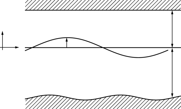
Figure 1.1: Internal gravity waves

We assume that the waters in the upper and the lower layers are both incompressible and inviscid fluids with constant densities $\rho_{1}$ and $\rho_{2}$, respectively, and that the flows are both irrotational. Then, the motion of the waters is described by the velocity potentials $\Phi_{1}(\bm{x},z,t)$ and $\Phi_{2}(\bm{x},z,t)$ and the pressures $P_{1}(\bm{x},z,t)$ and $P_{2}(\bm{x},z,t)$ in the upper and the lower layers. We recall the governing equations, referred as the full model for interfacial gravity waves, in Section 2 below. Generalizing the work of J. C. Luke [15], these equations can be obtained as the Euler–Lagrange equations associated with the Lagrangian density $\mathscr{L}(\Phi_{1},\Phi_{2},\zeta)$ given by the vertical integral of the pressure in both water regions. Building on this variational structure, T. Kakinuma [9, 10, 11] proposed and studied numerically the model obtained as the Euler–Lagrange equations for an approximated Lagrangian density, $\mathscr{L}(\Phi_{1}^{\mathrm{app}},\Phi_{2}^{\mathrm{app}},\zeta)$, where

(1.1) $$\Phi_{\ell}^{\mathrm{app}}(\bm{x},z,t)=\sum_{i=0}^{N_{\ell}}Z_{\ell,i}(z;\tilde{h}_{\ell}(\bm{x}))\phi_{\ell,i}(\bm{x},t)$$

for $\ell=1,2$, and $\{Z_{1,i}\}$ and $\{Z_{2,i}\}$ are appropriate function systems in the vertical coordinate $z$ and may depend on $\tilde{h}_{1}(\bm{x})$ and $\tilde{h}_{2}(\bm{x})$, respectively, which are thickness of the upper and the lower layers in the rest state, whereas $\bm{\phi}_{\ell}=(\phi_{\ell,0},\phi_{\ell,1},\ldots,\phi_{\ell,N_{\ell}})^{\mathrm{T}}$, $\ell=1,2$, are unknown variables. This yields a coupled system of equations for $\bm{\phi}_{1}$, $\bm{\phi}_{2}$, and $\zeta$, depending on the function systems $\{Z_{1,i}\}$ and $\{Z_{2,i}\}$, which we named Kakinuma model. Note that in our setting of the problem we have $\tilde{h}_{1}(\bm{x})=h_{1}$ and $\tilde{h}_{2}(\bm{x})=h_{2}-b(\bm{x})$.

The Kakinuma model is an extension to interfacial gravity waves of the so-called Isobe–Kakinuma model for surface gravity waves, that is, water waves, in which Luke’s Lagrangian density $\mathscr{L}_{\mathrm{Luke}}(\Phi,\zeta)$, where $\zeta$ is the surface elevation and $\Phi$ is the velocity potential of the water, is approximated by a density $\mathscr{L}^{\mathrm{app}}(\bm{\phi},\zeta)=\mathscr{L}_{\mathrm{Luke}}(\Phi^{\mathrm{app}},\zeta)$, where

(1.2) $$\Phi^{\mathrm{app}}(\bm{x},z,t)=\sum_{i=0}^{N}Z_{i}(z;b(\bm{x}))\phi_{i}(\bm{x},t).$$

The Isobe–Kakinuma model was first proposed by M. Isobe [7, 8] and then applied by T. Kakinuma to simulate numerically the water waves. Recently, this model was analyzed from a mathematical point of view when the function system $\{Z_{i}\}$ is a set of polynomials in $z$: $Z_{i}(z;b(\bm{x}))=(z+h-b(\bm{x}))^{p_{i}}$ with integers $p_{i}$ satisfying $0=p_{0}<p_{1}<\cdots<p_{N}$. The initial value problem was analyzed by Y. Murakami and T. Iguchi [16] in a special case and by R. Nemoto and T. Iguchi [17] in the general case. The hypersurface $t=0$ in the space-time $\mathbf{R}^{n}\times\mathbf{R}$ is characteristic for the Isobe–Kakinuma model, so that one needs to impose some compatibility conditions on the initial data for the existence of the solution. Under these compatibility conditions, the non-cavitation condition, and a Rayleigh–Taylor type condition $-\partial_{z}P^{\mathrm{app}}\geq c_{0}>0$ on the water surface, where $P^{\mathrm{app}}$ is an approximate pressure in the Isobe–Kakinuma model calculated from Bernoulli’s equation, they showed the well-posedness of the initial value problem in Sobolev spaces locally in time. Moreover, T. Iguchi [5, 6] showed that under the choice of the function system

(1.3) $$Z_{i}(z;b(\bm{x}))=\begin{cases}(z+h)^{2i}&\mbox{in the case of the flat bottom},\\ (z+h-b(\bm{x}))^{i}&\mbox{in the case of a variable bottom},\end{cases}$$

the Isobe–Kakinuma model is a higher order shallow water approximation for the water wave problem in the strongly nonlinear regime. Furthermore, V. Duchêne and T. Iguchi [2] showed that the Isobe–Kakinuma model also enjoys a Hamiltonian structure analogous to the one exhibited by V. E. Zakharov [19] on the full water wave problem and that the Hamiltonian of the Isobe–Kakinuma model is a higher order shallow water approximation to the one of the full water wave problem.

Our aim in the present paper and the companion paper [3] is to extend these results on surface gravity waves to the framework of interfacial gravity waves. In [3], we analyzed the Cauchy problem for Kakinuma model when the approximated velocity potentials are defined by

(1.4) $$\begin{cases}\displaystyle\Phi_{1}^{\mathrm{app}}(\bm{x},z,t):=\sum_{i=0}^{N}(-z+h_{1})^{2i}\phi_{1,i}(\bm{x},t),\\[10.76385pt] \displaystyle\Phi_{2}^{\mathrm{app}}(\bm{x},z,t):=\sum_{i=0}^{N^{*}}(z+h_{2}-b(\bm{x}))^{p_{i}}\phi_{2,i}(\bm{x},t),\end{cases}$$

where $N,N^{*}$, and $p_{0},p_{1},\ldots,p_{N^{*}}$ are nonnegative integers satisfying ${0=p_{0}<p_{1}<\cdots<p_{N^{*}}}$. We found that contrary to the full model for interfacial gravity waves, the Kakinuma model has a stability regime which can be expressed as

(1.5) $$-\partial_{z}(P_{2}^{\mathrm{app}}-P_{1}^{\mathrm{app}})-\frac{\rho_{1}\rho_{2}}{\rho_{1}H_{2}\alpha_{2}+\rho_{2}H_{1}\alpha_{1}}|\nabla\Phi_{2}^{\mathrm{app}}-\nabla\Phi_{1}^{\mathrm{app}}|^{2}\geq c_{0}>0$$

on the interface, where $P_{1}^{\mathrm{app}}$ and $P_{2}^{\mathrm{app}}$ are approximate pressures of the waters in the upper and the lower layers, $\alpha_{1}$ and $\alpha_{2}$ are positive constants depending only on $N$ and on $p_{0},p_{1},\ldots,p_{N^{*}}$, respectively. This is a generalization of the aforementioned Rayleigh–Taylor type condition for the Isobe–Kakinuma model. Moreover, when the motion of the waters together with the motion of the interface is in the rest state, the above stability condition is reduced to the well-known stable stratification condition

(1.6) $$(\rho_{2}-\rho_{1})g>0.$$

In [3], we showed that under the stability condition (1.5), the non-cavitation assumptions, and intrinsic compatibility conditions on the initial data, the initial value problem for the Kakinuma model is well-posed in Sobolev spaces locally in time. It is worth noticing that the constants $\alpha_{1}$ and $\alpha_{2}$ converge to $0$ as $N$ and $N^{*}$ go to infinity so that the stability condition becomes more and more stringent as $N$ and $N^{*}$ grow. However, this is consistent with the fact that the initial value problem for the full model for interfacial gravity waves is ill-posed in Sobolev spaces; see T. Iguchi, N. Tanaka, and A. Tani [18], V. Kamotski and G. Lebeau [12] and D. Lannes [13]. We also showed in [3] that the Kakinuma model enjoys a Hamiltonian structure analogous to the one exhibited by T. B. Benjamin and T. J. Bridges [1] on the full model for interfacial gravity waves. In the present paper we will complete the analysis by showing that the Kakinuma model obtained through the approximated potentials (1.4) with

1. $N^{*}=N$ and $p_{i}=2i$ $(i=0,1,\ldots,N)$ in the case of the flat bottom $b(\bm{x})\equiv 0$,

2. $N^{*}=2N$ and $p_{i}=i$ $(i=0,1,\ldots,2N)$ in the case with general bottom topographies,

provides a higher order shallow water approximation to the full model for interfacial gravity waves in the strongly nonlinear regime. More precisely, we will show that, after suitable rescaling, the dimensionless Kakinuma model is consistent with the full model for interfacial gravity waves with an error of order $O(\delta_{1}^{4N+2}+\delta_{2}^{4N+2})$, where $\delta_{1}$ and $\delta_{2}$ are shallowness parameters related to the upper and the lower layers, respectively, that is, $\delta_{\ell}=\frac{h_{\ell}}{\lambda}$ $(\ell=1,2)$ with the typical horizontal wavelength $\lambda$. A full justification of the Kakinuma model as shallow water approximations is not straightforward, because one cannot expect to construct a solution to the initial value problem for the full model with a uniform bound for general initial data in Sobolev spaces due to the ill-posedness of the problem. Nevertheless, if we assume the existence of a solution to the full model with a uniform bound and the stability condition (1.5) for the initial data, then we can show the existence of a corresponding solution to the Kakinuma model with appropriate initial data and the error estimate

$$|\zeta^{\mbox{\rm\tiny K}}(\bm{x},t)-\zeta^{\mbox{\rm\tiny IW}}(\bm{x},t)|\lesssim\delta_{1}^{4N+2}+\delta_{2}^{4N+2}$$

on some time interval independent of $\delta_{1}$ and $\delta_{2}$, where $\zeta^{\mbox{\rm\tiny K}}$ and $\zeta^{\mbox{\rm\tiny IW}}$ are solutions to the dimensionless Kakinuma model and to the full model, respectively. Moreover, under an appropriate assumption on the canonical variables $(\zeta,\phi)$, we show the error estimate

$$|\mathscr{H}^{\mbox{\rm\tiny K}}(\zeta,\phi)-\mathscr{H}^{\mbox{\rm\tiny IW}}(\zeta,\phi)|\lesssim\delta_{1}^{4N+2}+\delta_{2}^{4N+2},$$

where $\mathscr{H}^{\mbox{\rm\tiny K}}$ and $\mathscr{H}^{\mbox{\rm\tiny IW}}$ are Hamiltonians of the Kakinuma model and of the full model, respectively. Our error bounds in this paper are uniform with respect to the positive densities $\rho_{1}$ and $\rho_{2}$ satisfying the stable stratification condition $(\rho_{2}-\rho_{1})g>0$ and positive mean thicknesses of the upper layer $h_{1}$ and of the lower layer $h_{2}$ in the following two regimes: (i) $\rho_{1}\simeq\rho_{2}$; (ii) $\rho_{1}\ll\rho_{2}$ and $h_{2}\lesssim h_{1}$. In other words, in addition to assuming the stable stratification condition, the regime (iii) $\rho_{1}\ll\rho_{2}$ and $h_{1}\ll h_{2}$ will be excluded in this paper.

The contents of this paper are as follows. In Section 2 we first recall the basic equations governing the interfacial gravity waves and write down the Kakinuma model that we are going to analyze in this paper, and then rewrite them in a nondimensional form by introducing several nondimensional parameters. Hamiltonians of the full model and of the Kakinuma model in the nondimensional variables are also provided. In Section 3 we first introduce some differential operators, which enable us to write the Kakinuma model in a simple form, and then we present our main results in this paper: Theorem 3.1 ensures the existence of the solution to the initial value problem for the Kakinuma model on a time interval independent of parameters, especially, $\delta_{1}$ and $\delta_{2}$, under the stability condition, the non-cavitation assumptions, and intrinsic compatibility conditions on the initial data, together with a uniform bound of the solution; Remark 3.2 and Proposition 3.3 explain how to prepare the initial data for the Kakinuma model, which have to satisfy the compatibility conditions; Theorems 3.4 and 3.5 ensure the consistency of the Kakinuma model to the full model; More precisely, Theorem 3.4 states that the solutions to the Kakinuma model satisfy approximately the full model with an error of order $O(\delta_{1}^{4N+2}+\delta_{2}^{4N+2})$; Conversely, Theorem 3.5 states that the solutions to the full model satisfy approximately the Kakinuma model with an error of the same order; Theorem 3.8 gives conditionally a rigorous justification of the Kakinuma model, that is, assuming the existence of a solution to the full model with a uniform bound we derive an error estimate between a corresponding solution to the Kakinuma model and that of the full model; Finally, Theorem 3.9 gives an error estimate between the Hamiltonian of the Kakinuma model and that of the full model. In Section 4 we first remind results in the framework of surface waves related to the consistency of the Isobe–Kakinuma model, and then prove Theorems 3.4 and 3.5 by a simple scaling argument. In Section 5 we first derive an elliptic estimate related to the compatibility conditions, and then give uniform a priori bounds on regular solutions to the Kakinuma model, especially, a priori bounds of time derivatives. In Section 6 we provide uniform energy estimates for the solution to the Kakinuma model and prove Theorem 3.1. In Section 7 we first give a supplementary estimate on an approximation of the Dirichlet-to-Neumann map, and then revisit the consistency of the Kakinuma model. We prove Proposition 7.6, which is another version of the consistency given in Theorem 3.5, where we adopt a different construction of an approximate solution to the Kakinuma model from the solution to the full model. Then, by making use of the well-posedness of the initial value problem for the Kakinuma model we prove Theorem 3.8 a conditional rigorous justification of the Kakinuma model. Finally, in Section 8 we prove Theorem 3.9 on the approximation of the Hamiltonian.

Notation.  We denote by $W^{m,p}$ the $L^{p}$ Sobolev space of order $m$ on $\mathbf{R}^{n}$ and $H^{m}=W^{m,2}$. We put $\mathring{H}^{m}=\{\phi\,;\,\nabla\phi\in H^{m-1}\}$. The norm of a Banach space $B$ is denoted by $\|\cdot\|_{B}$. The $L^{2}$-inner product is denoted by $(\cdot,\cdot)_{L^{2}}$. We put $\partial_{t}=\frac{\partial}{\partial t}$, $\partial_{j}=\partial_{x_{j}}=\frac{\partial}{\partial x_{j}}$, and $\partial_{z}=\frac{\partial}{\partial z}$. $[P,Q]=PQ-QP$ denotes the commutator and $[P;u,v]=P(uv)-(Pu)v-u(Pv)$ denotes the symmetric commutator. For a matrix $A$ we denote by $A^{\mathrm{T}}$ the transpose of $A$. $O$ denotes a zero matrix. For a vector $\mbox{\boldmath$\phi$}=(\phi_{0},\phi_{1},\ldots,\phi_{N})^{\mathrm{T}}$ we denote the last $N$ components by $\mbox{\boldmath$\phi$}^{\prime}=(\phi_{1},\ldots,\phi_{N})^{\mathrm{T}}$. We use the notational convention $\frac{0}{0}=0$. $f\lesssim g$ means that there exists a non-essential positive constant $C$ such that $f\leq Cg$ holds. $f\simeq g$ means that $f\lesssim g$ and $g\lesssim f$ hold.

Acknowledgement
T. I. was partially supported by JSPS KAKENHI Grant Number JP17K18742 and JP22H01133. V. D. thanks the Centre Henri Lebesgue ANR-11-LABX-0020-01 for creating an attractive mathematical environment.

2 The basic equations and the Kakinuma model

2.1 Equations with physical variables

We first recall the equations governing potential flows for two layers of immiscible, incompressible, homogeneous, and inviscid fluids, and then write down the Kakinuma model at stake in this work. In the following, we denote the upper layer, the lower layer, the interface, the rigid-lid, and the bottom at time t by $\Omega_{1}(t)$, $\Omega_{2}(t)$, $\Gamma(t)$, $\Sigma_{1}$, and $\Sigma_{2}$, respectively. The velocity potentials $\Phi_{1}(\bm{x},z,t)$ and $\Phi_{2}(\bm{x},z,t)$ in the upper and lower layers, respectively, satisfy Laplace’s equations

(2.1) $$\Delta\Phi_{1}+\partial_{z}^{2}\Phi_{1}=0\quad\mbox{in}\quad\Omega_{1}(t),$$

(2.2) $$\Delta\Phi_{2}+\partial_{z}^{2}\Phi_{2}=0\quad\mbox{in}\quad\Omega_{2}(t),$$

where $\Delta=\partial_{1}^{2}+\cdots+\partial_{n}^{2}$ is the Laplacian with respect to the horizontal space variables $\bm{x}=(x_{1},\ldots,x_{n})$. Bernoulli’s laws of each layers have the form

(2.3) $$\rho_{1}\left(\partial_{t}\Phi_{1}+\frac{1}{2}(|\nabla\Phi_{1}|^{2}+(\partial_{z}\Phi_{1})^{2})+gz\right)+P_{1}=0\quad\mbox{in}\quad\Omega_{1}(t),$$

(2.4) $$\rho_{2}\left(\partial_{t}\Phi_{2}+\frac{1}{2}(|\nabla\Phi_{2}|^{2}+(\partial_{z}\Phi_{2})^{2})+gz\right)+P_{2}=0\quad\mbox{in}\quad\Omega_{2}(t),$$

where $\nabla=(\partial_{1},\ldots,\partial_{n})$, the positive constant $g$ is the acceleration due to gravity, and $P_{1}(\bm{x},z,t)$ and $P_{2}(\bm{x},z,t)$ are pressures in the upper and lower layers, respectively. The dynamical boundary condition on the interface is given by

(2.5) $$P_{1}=P_{2}\quad\mbox{on}\quad\Gamma(t).$$

The kinematic boundary conditions on the interface, the rigid-lid, and the bottom are given by

(2.6) $$\partial_{t}\zeta+\nabla\Phi_{1}\cdot\nabla\zeta-\partial_{z}\Phi_{1}=0\quad\mbox{on}\quad\Gamma(t),$$

(2.7) $$\partial_{t}\zeta+\nabla\Phi_{2}\cdot\nabla\zeta-\partial_{z}\Phi_{2}=0\quad\mbox{on}\quad\Gamma(t),$$

(2.8) $$\partial_{z}\Phi_{1}=0\makebox[78.79143pt]{}\quad\mbox{on}\quad\Sigma_{1},$$

(2.9) $$\nabla\Phi_{2}\cdot\nabla b-\partial_{z}\Phi_{2}=0\makebox[27.12492pt]{}\quad\mbox{on}\quad\Sigma_{2}.$$

These are the basic equations for interfacial gravity waves. It follows from Bernoulli’s laws (2.3)–(2.4) and the dynamical boundary condition (2.5) that

(2.10) $$\rho_{1}\left(\partial_{t}\Phi_{1}+\frac{1}{2}(|\nabla\Phi_{1}|^{2}+(\partial_{z}\Phi_{1})^{2})\right)$$

$$-\rho_{2}\left(\partial_{t}\Phi_{2}+\frac{1}{2}(|\nabla\Phi_{2}|^{2}+(\partial_{z}\Phi_{2})^{2})\right)=(\rho_{2}-\rho_{1})g\zeta\quad\mbox{on}\quad\Gamma(t).$$

We will always assume the stable stratification condition $(\rho_{2}-\rho_{1})g>0$. As in the case of the surface water waves, the basic equations have a variational structure and the corresponding Luke’s Lagrangian is given, up to terms which do not contribute to the variation of the Lagrangian, by the vertical integral of the pressure in the water regions. After using Bernoulli’s laws (2.3)–(2.4) we can find the Lagrangian density

(2.11) $$\mathscr{L}(\Phi_{1},\Phi_{2},\zeta) =-\rho_{1}\int_{\zeta}^{h_{1}}\left(\partial_{t}\Phi_{1}+\frac{1}{2}(|\nabla\Phi_{1}|^{2}+(\partial_{z}\Phi_{1})^{2})\right){\rm d}z$$

$$\quad\;-\rho_{2}\int_{-h_{2}+b}^{\zeta}\left(\partial_{t}\Phi_{2}+\frac{1}{2}(|\nabla\Phi_{2}|^{2}+(\partial_{z}\Phi_{2})^{2})\right){\rm d}z-\frac{1}{2}(\rho_{2}-\rho_{1})g\zeta^{2}.$$

In fact, one checks readily that (2.1)–(2.2) and (2.6)–(2.10) are Euler–Lagrange equations associated with the action function

$$\mathscr{J}(\Phi_{1},\Phi_{2},\zeta):=\int_{t_{0}}^{t_{1}}\!\!\!\int_{\mathbf{R}^{n}}\mathscr{L}(\Phi_{1},\Phi_{2},\zeta)\,\mathrm{d}\bm{x}\,\mathrm{d}t.$$

We proceed to the Kakinuma model. Let $N$ and $N^{*}$ be nonnegative integers. In view of the analysis for the Isobe–Kakinuma model for surface water waves, we approximate the velocity potentials $\Phi_{1}$ and $\Phi_{2}$ in the Lagrangian by

(2.12) $$\begin{cases}\displaystyle\Phi_{1}^{\mathrm{app}}(\bm{x},z,t)=\sum_{i=0}^{N}(-z+h_{1})^{2i}\phi_{1,i}(\bm{x},t),\\[10.76385pt] \displaystyle\Phi_{2}^{\mathrm{app}}(\bm{x},z,t)=\sum_{i=0}^{N^{*}}(z+h_{2}-b(\bm{x}))^{p_{i}}\phi_{2,i}(\bm{x},t),\end{cases}$$

where $p_{0},p_{1},\ldots,p_{N^{*}}$ are nonnegative integers satisfying $0=p_{0}<p_{1}<\cdots<p_{N^{*}}$. Plugging (2.12) into the Lagrangian density (2.11), we obtain an approximate Lagrangian density

$$\mathscr{L}^{\mathrm{app}}(\bm{\phi}_{1},\bm{\phi}_{2},\zeta):=\mathscr{L}(\Phi_{1}^{\mathrm{app}},\Phi_{2}^{\mathrm{app}},\zeta),$$

where $\bm{\phi}_{1}:=(\phi_{1,0},\phi_{1,1},\ldots,\phi_{1,N})^{\mathrm{T}}$ and $\bm{\phi}_{2}:=(\phi_{2,0},\phi_{2,1},\ldots,\phi_{2,N^{*}})^{\mathrm{T}}$. The corresponding Euler–Lagrange equation is the Kakinuma model, which has the form

(2.13) $$\begin{cases}\displaystyle H_{1}^{2i}\partial_{t}\zeta-\sum_{j=0}^{N}\biggl{\{}\nabla\cdot\biggr{(}\frac{1}{2(i+j)+1}H_{1}^{2(i+j)+1}\nabla\phi_{1,j}\biggr{)}-\frac{4ij}{2(i+j)-1}H_{1}^{2(i+j)-1}\phi_{1,j}\biggr{\}}=0\\ \makebox[270.00041pt]{}\mbox{for}\quad i=0,1,\ldots,N,\\ \displaystyle H_{2}^{p_{i}}\partial_{t}\zeta+\sum_{j=0}^{N^{*}}\biggl{\{}\nabla\cdot\biggl{(}\frac{1}{p_{i}+p_{j}+1}H_{2}^{p_{i}+p_{j}+1}\nabla\phi_{2,j}-\frac{p_{j}}{p_{i}+p_{j}}H_{2}^{p_{i}+p_{j}}\phi_{2,j}\nabla b\biggr{)}\\ \displaystyle\phantom{H_{2}^{p_{i}}\partial_{t}\zeta+\sum_{j=0}^{N}}+\frac{p_{i}}{p_{i}+p_{j}}H_{2}^{p_{i}+p_{j}}\nabla b\cdot\nabla\phi_{2,j}-\frac{p_{i}p_{j}}{p_{i}+p_{j}-1}H_{2}^{p_{i}+p_{j}-1}(1+|\nabla b|^{2})\phi_{2,j}\biggr{\}}=0\\ \makebox[270.00041pt]{}\mbox{for}\quad i=0,1,\ldots,N^{*},\\ \displaystyle\rho_{1}\biggl{\{}\sum_{j=0}^{N}H_{1}^{2j}\partial_{t}\phi_{1,j}+g\zeta+\frac{1}{2}\biggl{(}\biggl{|}\sum_{j=0}^{N}H_{1}^{2j}\nabla\phi_{1,j}\biggr{|}^{2}+\biggl{(}\sum_{j=0}^{N}2jH_{1}^{2j-1}\phi_{1,j}\biggr{)}^{2}\biggr{)}\biggr{\}}\\ \displaystyle\quad-\rho_{2}\biggl{\{}\sum_{j=0}^{N^{*}}H_{2}^{p_{j}}\partial_{t}\phi_{2,j}+g\zeta\\ \displaystyle\qquad\quad+\frac{1}{2}\biggl{(}\biggl{|}\sum_{j=0}^{N^{*}}(H_{2}^{p_{j}}\nabla\phi_{2,j}-p_{j}H_{2}^{p_{j}-1}\phi_{2,j}\nabla b)\biggr{|}^{2}+\biggl{(}\sum_{j=0}^{N^{*}}p_{j}H_{2}^{p_{j}-1}\phi_{2,j}\biggr{)}^{2}\biggr{)}\biggr{\}}=0,\end{cases}$$

where $H_{1}$ and $H_{2}$ are thicknesses of the upper and the lower layers, that is,

$$H_{1}(t,\bm{x}):=h_{1}-\zeta(\bm{x},t),\qquad H_{2}(\bm{x},t):=h_{2}+\zeta(\bm{x},t)-b(\bm{x}).$$

Here and in what follows we use the notational convention $0/0=0$.

2.2 The dimensionless equations

In order to rigorously validate the Kakinuma model (2.13) as a higher order shallow water approximation of the full model for interfacial gravity waves (2.1)–(2.9), we first introduce nondimensional parameters and then non-dimensionalize the equations, through a convenient rescaling of variables. Let $\lambda$ be a typical horizontal wavelength. Following D. Lannes [13], we introduce a nondimensional parameter $\delta$ by

$$\delta:=\frac{h}{\lambda}\qquad\mbox{with}\quad h:=\frac{h_{1}h_{2}}{\underline{\rho}_{1}h_{2}+\underline{\rho}_{2}h_{1}},$$

where $\underline{\rho}_{1}$ and $\underline{\rho}_{2}$ are relative densities. We also need to use relative thicknesses $\underline{h}_{1}$ and $\underline{h}_{2}$ of the layers. These nondimensional parameters are defined by

$$\underline{\rho}_{\ell}:=\frac{\rho_{\ell}}{\rho_{1}+\rho_{2}},\qquad\underline{h}_{\ell}:=\frac{h_{\ell}}{h}\qquad(\ell=1,2),$$

which satisfy the relations

(2.14) $$\underline{\rho}_{1}+\underline{\rho}_{2}=1,\qquad\frac{\underline{\rho}_{1}}{\underline{h}_{1}}+\frac{\underline{\rho}_{2}}{\underline{h}_{2}}=1.$$

Note also that $\min\{h_{1},h_{2}\}\leq h\leq\max\{h_{1},h_{2}\}$. It follows from the second relation in (2.14) that

(2.15) $$1<\min\biggl{\{}\frac{\underline{h}_{1}}{\underline{\rho}_{1}},\frac{\underline{h}_{2}}{\underline{\rho}_{2}}\biggr{\}}\leq 2.$$

Here, we note that the standard shallowness parameters $\delta_{1}:=\frac{h_{1}}{\lambda}$ and $\delta_{2}:=\frac{h_{2}}{\lambda}$ relative to the upper and the lower layers, respectively, are related to the above parameters by $\delta_{\ell}=\underline{h}_{\ell}\delta$ for $\ell=1,2$. In many results of this paper, we restrict our consideration to the parameter regime

(2.16) $$\underline{h}_{1}^{-1},\underline{h}_{2}^{-1}\lesssim 1.$$

To understand this restriction, it is convenient to use nondimensional parameters $\gamma:=\frac{\rho_{1}}{\rho_{2}}$ and $\theta:=\frac{h_{1}}{h_{2}}$. In terms of these parameters, $\underline{h}_{\ell}^{-1}$ $(\ell=1,2)$ can be represented as

$$\underline{h}_{1}^{-1}=\frac{\gamma+1}{\gamma+\theta},\qquad\underline{h}_{2}^{-1}=\frac{\gamma^{-1}+1}{\gamma^{-1}+\theta^{-1}}.$$

Therefore, the only cases that (2.16) excludes are the case $\gamma,\theta\ll 1$ and the case $\gamma,\theta\gg 1$. Since we shall also assume the stable stratification condition $(\rho_{2}-\rho_{1})g>0$, we can describe the two regimes considered in this paper as

1. $\gamma\simeq 1$, i.e., $\rho_{1}\simeq\rho_{2}$,

2. $\gamma\ll 1$ and $\theta\gtrsim 1$, i.e., $\rho_{1}\ll\rho_{2}$ and $h_{2}\lesssim h_{1}$.

Introducing $c_{\mbox{\rm\tiny SW}}:=\sqrt{(\underline{\rho}_{2}-\underline{\rho}_{1})gh}$ the speed of infinitely long and small interfacial gravity waves, we rescale the independent and the dependent variables by

$$\bm{x}=\lambda\tilde{\bm{x}},\quad z=h\tilde{z},\quad t=\frac{\lambda}{c_{\mbox{\rm\tiny SW}}}\tilde{t},\quad\zeta=h\tilde{\zeta},\quad b=h\tilde{b},\quad\Phi_{\ell}=\lambda c_{\mbox{\rm\tiny SW}}\tilde{\Phi}_{\ell}\quad(\ell=1,2).$$

Plugging these into the full model (2.1)–(2.2) and (2.6)–(2.10) and dropping the tilde sign in the notation we obtain

$$\begin{cases}\Delta\Phi_{1}+\delta^{-2}\partial_{z}^{2}\Phi_{1}=0&\mbox{in}\quad\Omega_{1}(t),\\ \Delta\Phi_{2}+\delta^{-2}\partial_{z}^{2}\Phi_{2}=0&\mbox{in}\quad\Omega_{2}(t),\\ \partial_{t}\zeta+\nabla\Phi_{1}\cdot\nabla\zeta-\delta^{-2}\partial_{z}\Phi_{1}=0&\mbox{on}\quad\Gamma(t),\\ \partial_{t}\zeta+\nabla\Phi_{2}\cdot\nabla\zeta-\delta^{-2}\partial_{z}\Phi_{2}=0&\mbox{on}\quad\Gamma(t),\\ \partial_{z}\Phi_{1}=0&\mbox{on}\quad\Sigma_{1},\\ \nabla\Phi_{2}\cdot\nabla b-\delta^{-2}\partial_{z}\Phi_{2}=0&\mbox{on}\quad\Sigma_{2},\\ \underline{\rho}_{1}\Bigl{(}\partial_{t}\Phi_{1}+\frac{1}{2}|\nabla\Phi_{1}|^{2}+\frac{1}{2}\delta^{-2}(\partial_{z}\Phi_{1})^{2}\Bigr{)}\\ \quad-\underline{\rho}_{2}\Bigl{(}\partial_{t}\Phi_{2}+\frac{1}{2}|\nabla\Phi_{2}|^{2}+\frac{1}{2}\delta^{-2}(\partial_{z}\Phi_{2})^{2}\Bigr{)}-\zeta=0&\mbox{on}\quad\Gamma(t),\end{cases}$$

where in this scaling the upper layer $\Omega_{1}(t)$, the lower layer $\Omega_{2}(t)$, the interface $\Gamma(t)$, the rigid-lid $\Sigma_{1}$, and the bottom $\Sigma_{2}$ are written as

$$\Omega_{1}(t)=\{X=(\bm{x},z)\in\mathbf{R}^{n+1}\,;\,\zeta(\bm{x},t)<z<\underline{h}_{1}\},$$

$$\Omega_{2}(t)=\{X=(\bm{x},z)\in\mathbf{R}^{n+1}\,;\,-\underline{h}_{2}+b(\bm{x})<z<\zeta(\bm{x},t)\},$$

$$\Gamma(t)=\{X=(\bm{x},z)\in\mathbf{R}^{n+1}\,;\,z=\zeta(\bm{x},t)\},$$

$$\Sigma_{1}=\{X=(\bm{x},z)\in\mathbf{R}^{n+1}\,;\,z=\underline{h}_{1}\},$$

$$\Sigma_{2}=\{X=(\bm{x},z)\in\mathbf{R}^{n+1}\,;\,z=-\underline{h}_{2}+b(\bm{x})\}.$$

Denoting

$$\phi_{\ell}(\bm{x},t):=\Phi_{\ell}(\bm{x},\zeta(\bm{x},t),t)\qquad(\ell=1,2)$$

and using the chain rule, the above system can be written in a more compact and closed form as

(2.17) $$\begin{cases}\partial_{t}\zeta+\Lambda_{1}(\zeta,\delta,\underline{h}_{1})\phi_{1}=0,\\ \partial_{t}\zeta-\Lambda_{2}(\zeta,b,\delta,\underline{h}_{2})\phi_{2}=0,\\ \displaystyle\underline{\rho}_{1}\biggl{(}\partial_{t}\phi_{1}+\frac{1}{2}|\nabla\phi_{1}|^{2}-\frac{1}{2}\delta^{2}\frac{(\Lambda_{1}(\zeta,\delta,\underline{h}_{1})\phi_{1}-\nabla\zeta\cdot\nabla\phi_{1})^{2}}{1+\delta^{2}|\nabla\zeta|^{2}}\biggr{)}\\ \displaystyle\quad-\underline{\rho}_{2}\biggl{(}\partial_{t}\phi_{2}+\frac{1}{2}|\nabla\phi_{2}|^{2}-\frac{1}{2}\delta^{2}\frac{(\Lambda_{2}(\zeta,b,\delta,\underline{h}_{2})\phi_{2}+\nabla\zeta\cdot\nabla\phi_{2})^{2}}{1+\delta^{2}|\nabla\zeta|^{2}}\biggr{)}-\zeta=0,\end{cases}$$

where $\Lambda_{1}(\zeta,\delta,\underline{h}_{1})$ and $\Lambda_{2}(\zeta,b,\delta,\underline{h}_{2})$ are the Dirichlet-to-Neumann maps for Laplace’s equations. More precisely, these are defined by

$$\Lambda_{1}(\zeta,\delta,\underline{h}_{1})\phi_{1}:=\bigl{(}-\delta^{-2}\partial_{z}\Phi_{1}+\nabla\Phi_{1}\cdot\nabla\zeta\bigr{)}\bigr{|}_{z=\zeta(\bm{x},t)},$$

$$\Lambda_{2}(\zeta,b,\delta,\underline{h}_{2})\phi_{2}:=\bigl{(}\delta^{-2}\partial_{z}\Phi_{2}-\nabla\Phi_{2}\cdot\nabla\zeta\bigr{)}\bigr{|}_{z=\zeta(\bm{x},t)},$$

where $\Phi_{1}$ and $\Phi_{2}$ are unique solutions to the boundary value problems

$$\begin{cases}\Delta\Phi_{1}+\delta^{-2}\partial_{z}^{2}\Phi_{1}=0&\mbox{in}\quad\Omega_{1}(t),\\ \Phi_{1}=\phi_{1}&\mbox{on}\quad\Gamma(t),\\ \partial_{z}\Phi_{1}=0&\mbox{on}\quad\Sigma_{1},\end{cases}\text{ and }\quad\begin{cases}\Delta\Phi_{2}+\delta^{-2}\partial_{z}^{2}\Phi_{2}=0&\mbox{in}\quad\Omega_{2}(t),\\ \Phi_{2}=\phi_{2}&\mbox{on}\quad\Gamma(t),\\ \nabla\Phi_{2}\cdot\nabla b-\delta^{-2}\partial_{z}\Phi_{2}=0&\mbox{on}\quad\Sigma_{2}.\end{cases}$$

As for the Kakinuma model, we introduce additionally the rescaled variables

$$\phi_{1,i}:=\frac{\lambda c_{\mbox{\rm\tiny SW}}}{h_{1}^{2i}}\tilde{\phi}_{1,i},\qquad\phi_{2,i}:=\frac{\lambda c_{\mbox{\rm\tiny SW}}}{h_{2}^{p_{i}}}\tilde{\phi}_{2,i}.$$

Plugging these and the previous scaling into the Kakinuma model (2.13) and dropping the tilde sign in the notation we obtain the Kakinuma model in the nondimensional form, which is written as

(2.18) $$\begin{cases}\displaystyle H_{1}^{2i}\partial_{t}\zeta-\underline{h}_{1}\sum_{j=0}^{N}\biggl{\{}\nabla\cdot\biggr{(}\frac{1}{2(i+j)+1}H_{1}^{2(i+j)+1}\nabla\phi_{1,j}\biggr{)}-\frac{4ij}{2(i+j)-1}H_{1}^{2(i+j)-1}(\underline{h}_{1}\delta)^{-2}\phi_{1,j}\biggr{\}}=0\\ \makebox[290.00044pt]{}\mbox{for}\quad i=0,1,\ldots,N,\\ \displaystyle H_{2}^{p_{i}}\partial_{t}\zeta+\underline{h}_{2}\sum_{j=0}^{N^{*}}\biggl{\{}\nabla\cdot\biggl{(}\frac{1}{p_{i}+p_{j}+1}H_{2}^{p_{i}+p_{j}+1}\nabla\phi_{2,j}-\frac{p_{j}}{p_{i}+p_{j}}H_{2}^{p_{i}+p_{j}}\phi_{2,j}\underline{h}_{2}^{-1}\nabla b\biggr{)}\\ \displaystyle\qquad+\frac{p_{i}}{p_{i}+p_{j}}H_{2}^{p_{i}+p_{j}}\underline{h}_{2}^{-1}\nabla b\cdot\nabla\phi_{2,j}-\frac{p_{i}p_{j}}{p_{i}+p_{j}-1}H_{2}^{p_{i}+p_{j}-1}((\underline{h}_{2}\delta)^{-2}+\underline{h}_{2}^{-2}|\nabla b|^{2})\phi_{2,j}\biggr{\}}=0\\ \makebox[290.00044pt]{}\mbox{for}\quad i=0,1,\ldots,N^{*},\\ \displaystyle\underline{\rho}_{1}\biggl{\{}\sum_{j=0}^{N}H_{1}^{2j}\partial_{t}\phi_{1,j}+\frac{1}{2}\biggl{(}\biggl{|}\sum_{j=0}^{N}H_{1}^{2j}\nabla\phi_{1,j}\biggr{|}^{2}+(\underline{h}_{1}\delta)^{-2}\biggl{(}\sum_{j=0}^{N}2jH_{1}^{2j-1}\phi_{1,j}\biggr{)}^{2}\biggr{)}\biggr{\}}\\ \displaystyle\qquad-\underline{\rho}_{2}\biggl{\{}\sum_{j=0}^{N^{*}}H_{2}^{2j}\partial_{t}\phi_{2,j}+\frac{1}{2}\biggl{(}\biggl{|}\sum_{j=0}^{N^{*}}(H_{2}^{p_{j}}\nabla\phi_{2,j}-p_{j}H_{2}^{p_{j}-1}\phi_{2,j}\underline{h}_{2}^{-1}\nabla b)\biggr{|}^{2}\\ \displaystyle\makebox[170.00026pt]{}+(\underline{h}_{2}\delta)^{-2}\biggl{(}\sum_{j=0}^{N^{*}}p_{j}H_{2}^{p_{j}-1}\phi_{2,j}\biggr{)}^{2}\biggr{)}\biggr{\}}-\zeta=0,\end{cases}$$

where

(2.19) $$H_{1}(\bm{x},t):=1-\underline{h}_{1}^{-1}\zeta(\bm{x},t),\qquad H_{2}(\bm{x},t):=1+\underline{h}_{2}^{-1}\zeta(\bm{x},t)-\underline{h}_{2}^{-1}b(\bm{x}).$$

We impose the initial conditions to the Kakinuma model of the form

(2.20) $$(\zeta,\bm{\phi}_{1},\bm{\phi}_{2})=(\zeta_{(0)},\bm{\phi}_{1(0)},\bm{\phi}_{2(0)})\makebox[30.00005pt]{at}t=0.$$

2.3 Hamiltonian structures

It is well-known that the full model for interfacial gravity waves has a conserved energy

$$\mathscr{E} :=\sum_{\ell=1,2}\iint_{\Omega_{\ell}(t)}\frac{1}{2}\underline{\rho}_{\ell}\bigl{(}|\nabla\Phi_{\ell}(\bm{x},z,t)|^{2}+\delta^{-2}(\partial_{z}\Phi_{\ell}(\bm{x},z,t))^{2}\bigr{)}\mathrm{d}\bm{x}\mathrm{d}z+\int_{\mathbf{R}^{n}}\frac{1}{2}\zeta(\bm{x},t)^{2}\mathrm{d}\bm{x}$$

$$=\sum_{\ell=1,2}\frac{1}{2}\underline{\rho}_{\ell}(\Lambda_{\ell}(\zeta)\phi_{\ell}(t),\phi_{\ell}(t))_{L^{2}}+\frac{1}{2}\|\zeta(t)\|_{L^{2}}^{2},$$

which is the total energy, that is, the sum of the kinetic energies of the waters in the upper and the lower layers and the potential energy due to the gravity. Here and in what follows, we denote simply $\Lambda_{1}(\zeta)=\Lambda_{1}(\zeta,\delta,\underline{h}_{1})$ and $\Lambda_{2}(\zeta)=\Lambda_{2}(\zeta,b,\delta,\underline{h}_{2})$. Moreover, T. B. Benjamin and T. J. Bridges [1] found that the full model can be written in Hamilton’s canonical form

$$\partial_{t}\zeta=\frac{\delta\mathscr{H}^{\mbox{\rm\tiny IW}}}{\delta\phi},\qquad\partial_{t}\phi=-\frac{\delta\mathscr{H}^{\mbox{\rm\tiny IW}}}{\delta\zeta},$$

where the canonical variable $\phi$ is defined by

(2.21) $$\phi=\underline{\rho}_{2}\phi_{2}-\underline{\rho}_{1}\phi_{1}$$

and the Hamiltonian $\mathscr{H}^{\mbox{\rm\tiny IW}}$ is the total energy $\mathscr{E}$ written in terms of the canonical variables $(\zeta,\phi)$. It follows from the kinematic boundary conditions on the interface that $\Lambda_{1}(\zeta)\phi_{1}+\Lambda_{2}(\zeta)\phi_{2}=0$, so that $\phi_{1}$ and $\phi_{2}$ can be written in terms of the canonical variables $(\zeta,\phi)$ as

$$\begin{cases}\phi_{1}=-(\underline{\rho}_{1}\Lambda_{2}(\zeta)+\underline{\rho}_{2}\Lambda_{1}(\zeta))^{-1}\Lambda_{2}(\zeta)\phi,\\ \phi_{2}=(\underline{\rho}_{1}\Lambda_{2}(\zeta)+\underline{\rho}_{2}\Lambda_{1}(\zeta))^{-1}\Lambda_{1}(\zeta)\phi.\end{cases}$$

Therefore, the Hamiltonian $\mathscr{H}^{\mbox{\rm\tiny IW}}(\zeta,\phi)$ of the full model for interfacial gravity waves is given explicitly by

$$\mathscr{H}^{\mbox{\rm\tiny IW}}(\zeta,\phi)=\frac{1}{2}((\underline{\rho}_{1}\Lambda_{2}(\zeta)+\underline{\rho}_{2}\Lambda_{1}(\zeta))^{-1}\Lambda_{1}(\zeta)\phi,\Lambda_{2}(\zeta)\phi)_{L^{2}}+\frac{1}{2}\|\zeta\|_{L^{2}}^{2}.$$

As was shown in the companion paper [3], the Kakinuma model (2.18) also enjoys a Hamiltonian structure analogous to that of the full model for interfacial gravity waves. The canonical variables are the elevation of the interface $\zeta$ and $\phi$ defined by

(2.22) $$\phi(\bm{x},t) :=\underline{\rho}_{2}\Phi_{2}^{\mathrm{app}}(\bm{x},\zeta(\bm{x},t),t)-\underline{\rho}_{1}\Phi_{1}^{\mathrm{app}}(\bm{x},\zeta(\bm{x},t),t)$$

$$=\underline{\rho}_{2}\sum_{i=0}^{N^{*}}H_{2}(\bm{x},t)^{p_{i}}\phi_{2,i}(\bm{x},t)-\underline{\rho}_{1}\sum_{i=0}^{N}H_{1}(\bm{x},t)^{2i}\phi_{1,i}(\bm{x},t),$$

where $\Phi_{\ell}^{\mathrm{app}}$ $(\ell=1,2)$ are nondimensional versions of the approximate velocity potentials, which are defined by

(2.23) $$\begin{cases}\displaystyle\Phi_{1}^{\mathrm{app}}(\bm{x},z,t):=\sum_{i=0}^{N}(1-\underline{h}_{1}^{-1}z)^{2i}\phi_{1,i}(\bm{x},t),\\[10.76385pt] \displaystyle\Phi_{2}^{\mathrm{app}}(\bm{x},z,t):=\sum_{i=0}^{N^{*}}(1+\underline{h}_{2}^{-1}(z-b(\bm{x})))^{p_{i}}\phi_{2,i}(\bm{x},t),\end{cases}$$

and $H_{\ell}$ $(\ell=1,2)$ are thicknesses of the upper and lower layers defined by (2.19). We note that if the canonical variables $(\zeta,\phi)$ are given, then the Kakinuma model (2.18) determines $\bm{\phi}_{1}=(\phi_{1,0},\phi_{1,1},\ldots,\phi_{1,N})^{\mathrm{T}}$ and $\bm{\phi}_{2}=(\phi_{2,0},\phi_{2,1},\ldots,\phi_{2,N^{*}})^{\mathrm{T}}$, which are unique up to an additive constant of the form $(\mathcal{C}\underline{\rho}_{1},\mathcal{C}\underline{\rho}_{2})$ to $(\phi_{1,0},\phi_{2,0})$. For details, we refer to [3, Subsection 8.1] and Lemma 5.1 in Section 5. Then, the Hamiltonian $\mathscr{H}^{\mbox{\rm\tiny K}}(\zeta,\phi)$ of the Kakinuma model is given by

$$\mathscr{H}^{\mbox{\rm\tiny K}}(\zeta,\phi) :=\sum_{\ell=1,2}\iint_{\Omega_{\ell}}\frac{1}{2}\underline{\rho}_{\ell}\bigl{(}|\nabla\Phi_{\ell}^{\mathrm{app}}(\bm{x},z,t)|^{2}+\delta^{-2}(\partial_{z}\Phi_{\ell}^{\mathrm{app}}(\bm{x},z,t))^{2}\bigr{)}\mathrm{d}\bm{x}\mathrm{d}z+\int_{\mathbf{R}^{n}}\frac{1}{2}\zeta(\bm{x},t)^{2}\mathrm{d}\bm{x}.$$

3 Statements of the main results

Before stating the main results in this paper, let us introduce some notations which allow in particular to rewrite (2.18) in a compact form. We introduce second order differential operators $L_{1,ij}=L_{1,ij}(H_{1},\delta,\underline{h}_{1})$ $(i,j=0,1,\ldots,N)$ and $L_{2,ij}=L_{2,ij}(H_{2},b,\delta,\underline{h}_{2})$ $(i,j=0,1,\ldots,N^{*})$ by

(3.1) $$L_{1,ij}\varphi_{1,j} :=-\nabla\cdot\biggl{(}\frac{1}{2(i+j)+1}H_{1}^{2(i+j)+1}\nabla\varphi_{1,j}\biggr{)}+\frac{4ij}{2(i+j)-1}H_{1}^{2(i+j)-1}(\underline{h}_{1}\delta)^{-2}\varphi_{1,j},$$

(3.2) $$L_{2,ij}\varphi_{2,j} :=-\nabla\cdot\biggl{(}\frac{1}{p_{i}+p_{j}+1}H_{2}^{p_{i}+p_{j}+1}\nabla\varphi_{2,j}-\frac{p_{j}}{p_{i}+p_{j}}H_{2}^{p_{i}+p_{j}}\varphi_{2,j}\underline{h}_{2}^{-1}\nabla b\biggr{)}$$

$$\quad\,-\frac{p_{i}}{p_{i}+p_{j}}H_{2}^{p_{i}+p_{j}}\underline{h}_{2}^{-1}\nabla b\cdot\nabla\varphi_{2,j}$$

$$\quad\,+\frac{p_{i}p_{j}}{p_{i}+p_{j}-1}H_{2}^{p_{i}+p_{j}-1}((\underline{h}_{2}\delta)^{-2}+\underline{h}_{2}^{-2}|\nabla b|^{2})\varphi_{2,j}.$$

Notice that we have $(L_{\ell,ij})^{*}=L_{\ell,ji}$ for $\ell=1,2$, where $(L_{\ell,ij})^{*}$ is the adjoint operator of $L_{\ell,ij}$ in $L^{2}(\mathbf{R}^{n})$. We put ${\bm{\phi}}_{1}:=(\phi_{1,0},\phi_{1,1},\ldots,\phi_{1,N})^{\mathrm{T}}$, ${\bm{\phi}}_{2}:=(\phi_{2,0},\phi_{2,1},\ldots,\phi_{2,N^{*}})^{\mathrm{T}}$, and

(3.3) $$\begin{cases}{\bm{l}}_{1}(H_{1}):=(1,H_{1}^{2},H_{1}^{4},\ldots,H_{1}^{2N})^{\mathrm{T}},\\ {\bm{l}}_{1}^{\prime}(H_{1}):=(0,2H_{1},\ldots,2NH_{1}^{2N-1})^{\mathrm{T}},\\ {\bm{l}}_{1}^{\prime\prime}(H_{1}):=(0,2,\ldots,2N(2N-1)H_{1}^{2N-2})^{\mathrm{T}},\\ {\bm{l}}_{2}(H_{2}):=(1,H_{2}^{p_{1}},H_{2}^{p_{2}},\ldots,H_{2}^{p_{N^{*}}})^{\mathrm{T}},\\ {\bm{l}}_{2}^{\prime}(H_{2}):=(0,p_{1}H_{2}^{p_{1}-1},\ldots,p_{N^{*}}H_{2}^{p_{N^{*}}})^{\mathrm{T}},\\ {\bm{l}}_{2}^{\prime\prime}(H_{2}):=(0,p_{1}(p_{1}-1)H_{2}^{p_{1}-2},\ldots,p_{N^{*}}(p_{N^{*}}-1)H_{2}^{p_{N^{*}}})^{\mathrm{T}},\end{cases}$$

and define ${\bm{u}}_{\ell}$ and $w_{\ell}$ for $\ell=1,2$, which represent approximately the horizontal and the vertical components of the velocity field on the interface from the water region $\Omega_{\ell}(t)$, by

(3.4) $$\left\{\begin{array}[]{ll}\displaystyle{\bm{u}}_{1}:=({\bm{l}}_{1}(H_{1})\otimes\nabla)^{\mathrm{T}}{\bm{\phi}}_{1},&\displaystyle w_{1}:=-{\bm{l}}_{1}^{\prime}(H_{1})\cdot{\bm{\phi}}_{1},\\ \displaystyle{\bm{u}}_{2}:=({\bm{l}}_{2}(H_{2})\otimes\nabla)^{\mathrm{T}}{\bm{\phi}}_{2}-({\bm{l}}_{2}^{\prime}(H_{2})\cdot{\bm{\phi}}_{2})\underline{h}_{2}^{-1}\nabla b,&\displaystyle w_{2}:={\bm{l}}_{2}^{\prime}(H_{2})\cdot{\bm{\phi}}_{2}.\end{array}\right.$$

Then, denoting $L_{1}:=(L_{1,ij})_{0\leq i,j\leq N}$ and $L_{2}:=(L_{2,ij})_{0\leq i,j\leq N^{*}}$ we can write the Kakinuma model (2.18) more compactly as

(3.5) $$\begin{cases}\displaystyle{\bm{l}}_{1}(H_{1})\partial_{t}\zeta+\underline{h}_{1}L_{1}(H_{1},\delta,\underline{h}_{1}){\bm{\phi}}_{1}={\bm{0}},\\ \displaystyle{\bm{l}}_{2}(H_{2})\partial_{t}\zeta-\underline{h}_{2}L_{2}(H_{2},b,\delta,\underline{h}_{2}){\bm{\phi}}_{2}={\bm{0}},\\ \underline{\rho}_{1}\bigl{\{}{\bm{l}}_{1}(H_{1})\cdot\partial_{t}{\bm{\phi}}_{1}+\frac{1}{2}\bigl{(}|{\bm{u}}_{1}|^{2}+(\underline{h}_{1}\delta)^{-2}w_{1}^{2}\bigr{)}\bigr{\}}\\ \quad-\underline{\rho}_{2}\bigl{\{}{\bm{l}}_{2}(H_{2})\cdot\partial_{t}{\bm{\phi}}_{2}+\frac{1}{2}\bigl{(}|{\bm{u}}_{2}|^{2}+(\underline{h}_{2}\delta)^{-2}w_{2}^{2}\bigr{)}\bigr{\}}-\zeta=0.\end{cases}$$

By eliminating $\partial_{t}\zeta$ from the Kakinuma model, we obtain $N+N^{*}+1$ scalar relations which are necessary conditions for the existence of the solution to the Kakinuma model, as stated below. Introducing linear operators $\mathcal{L}_{1,i}:=\mathcal{L}_{1,i}(H_{1},\delta,\underline{h}_{1})$ $(i=0,\ldots,N)$ acting on ${\bm{\varphi}}_{1}=(\varphi_{1,0},\ldots,\varphi_{1,N})^{\mathrm{T}}$ and $\mathcal{L}_{2,i}:=\mathcal{L}_{2,i}(H_{2},b,\delta,\underline{h}_{2})$ $(i=0,\ldots,N^{*})$ acting on ${\bm{\varphi}}_{2}=(\varphi_{2,0},\ldots,\varphi_{2,N^{*}})^{\mathrm{T}}$ by

(3.6) $$\begin{cases}\displaystyle\mathcal{L}_{1,0}{\bm{\varphi}}_{1}:=\sum_{j=0}^{N}L_{1,0j}\varphi_{1,j},\\ \displaystyle\mathcal{L}_{1,i}{\bm{\varphi}}_{1}:=\sum_{j=0}^{N}(L_{1,ij}\varphi_{1,j}-H_{1}^{2i}L_{1,0j}\varphi_{1,j})\quad\mbox{for}\quad i=1,2,\ldots,N,\\ \displaystyle\mathcal{L}_{2,0}{\bm{\varphi}}_{2}:=\sum_{j=0}^{N^{*}}L_{2,0j}\varphi_{2,j},\\ \displaystyle\mathcal{L}_{2,i}{\bm{\varphi}}_{2}:=\sum_{j=0}^{N^{*}}(L_{2,ij}\varphi_{2,j}-H_{2}^{p_{i}}L_{2,0j}\varphi_{2,j})\quad\mbox{for}\quad i=1,2,\ldots,N^{*},\end{cases}$$

the necessary conditions can be written simply as

(3.7) $$\begin{cases}\mathcal{L}_{1,i}(H_{1},\delta,\underline{h}_{1}){\bm{\phi}}_{1}=0\quad\mbox{for}\quad i=1,2,\ldots,N,\\ \mathcal{L}_{2,i}(H_{2},b,\delta,\underline{h}_{2}){\bm{\phi}}_{2}=0\quad\mbox{for}\quad i=1,2,\ldots,N^{*},\\ \underline{h}_{1}\mathcal{L}_{1,0}(H_{1},\delta,\underline{h}_{1}){\bm{\phi}}_{1}+\underline{h}_{2}\mathcal{L}_{2,0}(H_{2},b,\delta,\underline{h}_{2}){\bm{\phi}}_{2}=0.\end{cases}$$

Hereafter, these necessary conditions will be referred to as the compatibility conditions. Notice that under these compatibility conditions we have for $\ell=1,2$

(3.8) $$L_{\ell}\bm{\phi}_{\ell}=\bm{l}_{\ell}\mathcal{L}_{\ell,0}\bm{\phi}_{\ell},$$

where $\bm{l}_{\ell}=\bm{l}_{\ell}(H_{\ell})$ and similar simplifications of notations will be used in the following without any comments. In connection with the stability condition (1.5), we introduce a function

(3.9) $$a:=1 +\underline{\rho}_{1}\underline{h}_{1}^{-1}\{\bm{l}_{1}^{\prime}(H_{1})\cdot(\partial_{t}+\bm{u}_{1}\cdot\nabla)\bm{\phi}_{1}-(\underline{h}_{1}\delta)^{-2}w_{1}\bm{l}_{1}^{\prime\prime}(H_{1})\cdot\bm{\phi}_{1}\}$$

$$+\underline{\rho}_{2}\underline{h}_{2}^{-1}\{\bm{l}_{2}^{\prime}(H_{2})\cdot(\partial_{t}+\bm{u}_{2}\cdot\nabla)\bm{\phi}_{2}+\bigl{(}(\underline{h}_{2}\delta)^{-2}w_{2}-\underline{h}_{2}^{-1}\nabla b\cdot\bm{u}_{2}\bigr{)}\bm{l}_{2}^{\prime\prime}(H_{2})\cdot\bm{\phi}_{2}\},$$

which corresponds to $-(\partial_{z}(P_{2}^{\mathrm{app}}-P_{1}^{\mathrm{app}}))|_{\Gamma(t)}$ in the stability condition.

Our first main result in this paper is the existence of the solution to the initial value problem (2.18)–(2.20) for the Kakinuma model on a time interval independent of parameters, especially, the shallowness parameters $\delta_{1}=\underline{h}_{1}\delta$ and $\delta_{2}=\underline{h}_{2}\delta$ together with a uniform bound of the solution. For simplicity, we denote $H_{\ell(0)}:=H_{\ell}|_{t=0}$, $\bm{u}_{\ell(0)}:=\bm{u}_{\ell}|_{t=0}$ for $\ell=1,2$, and $a_{(0)}:=a|_{t=0}$, which can be written in terms of the initial data according to the initial condition (2.20). Although the function $a$ includes the terms $(\partial_{t}\bm{\phi}_{\ell}^{\prime})|_{t=0}$ for $\ell=1,2$, where $\bm{\phi}_{1}^{\prime}=(\phi_{1,1},\ldots,\phi_{1,N})^{\mathrm{T}}$ and $\bm{\phi}_{2}^{\prime}=(\phi_{2,1},\ldots,\phi_{2,N^{*}})^{\mathrm{T}}$, and the hypersurface $t=0$ is characteristic for the Kakinuma model, we can uniquely determine them in terms of the initial data. For details, we refer to Remark 5.3.

Theorem 3.1.

Let $c_{0},M_{0},\underline{h}_{\mathrm{min}}$ be positive constants and $m$ an integer such that ${m>\frac{n}{2}+1}$. There exist a time $T>0$ and a constant $M>0$ such that for any positive parameters $\underline{\rho}_{1},\underline{\rho}_{2},\underline{h}_{1},\underline{h}_{2},\delta$ satisfying the natural restrictions (2.14), $\underline{h}_{1}\delta,\underline{h}_{2}\delta\leq 1$, as well as the condition ${\underline{h}_{\mathrm{min}}\leq\underline{h}_{1},\underline{h}_{2}}$, if the initial data $(\zeta_{(0)},\bm{\phi}_{1(0)},\bm{\phi}_{2(0)})$ and the bottom topography $b$ satisfy

(3.10) $$\begin{cases}\displaystyle\|\zeta_{(0)}\|_{H^{m}}^{2}+\sum_{\ell=1,2}\underline{\rho}_{\ell}\underline{h}_{\ell}\bigl{(}\|\nabla\bm{\phi}_{\ell(0)}\|_{H^{m}}^{2}+(\underline{h}_{\ell}\delta)^{-2}\|\bm{\phi}_{\ell(0)}^{\prime}\|_{H^{m}}^{2}\bigr{)}\leq M_{0},\\ \underline{h}_{2}^{-1}\bigl{(}\|b\|_{W^{m+1,\infty}}+(\underline{h}_{2}\delta)\|b\|_{W^{m+2,\infty}}\bigr{)}\leq M_{0},\end{cases}$$

the non-cavitation assumption

(3.11) $$H_{1(0)}(\bm{x})\geq c_{0},\quad H_{2(0)}(\bm{x})\geq c_{0}\quad\mbox{for}\quad\bm{x}\in\mathbf{R}^{n},$$

the stability condition

(3.12) $$a_{(0)}(\bm{x})-\frac{\underline{\rho}_{1}\underline{\rho}_{2}}{\underline{\rho}_{1}\underline{h}_{2}H_{2(0)}(\bm{x})\alpha_{2}+\underline{\rho}_{2}\underline{h}_{1}H_{1(0)}(\bm{x})\alpha_{1}}|{\bm{u}}_{1(0)}(\bm{x})-{\bm{u}}_{2(0)}(\bm{x})|^{2}\geq c_{0}\quad\mbox{for}\quad\bm{x}\in\mathbf{R}^{n},$$

with positive constants $\alpha_{1}$ and $\alpha_{2}$ defined by (6.9), and the compatibility conditions

(3.13) $$\begin{cases}\mathcal{L}_{1,i}(H_{1(0)},\delta,\underline{h}_{1}){\bm{\phi}}_{1(0)}=0\quad\mbox{for}\quad i=1,2,\ldots,N,\\ \mathcal{L}_{2,i}(H_{2(0)},b,\delta,\underline{h}_{2}){\bm{\phi}}_{2(0)}=0\quad\mbox{for}\quad i=1,2,\ldots,N^{*},\\ \underline{h}_{1}\mathcal{L}_{1,0}(H_{1(0)},\delta,\underline{h}_{1}){\bm{\phi}}_{1(0)}+\underline{h}_{2}\mathcal{L}_{2,0}(H_{2(0)},b,\delta,\underline{h}_{2}){\bm{\phi}}_{2(0)}=0,\end{cases}$$

then the initial value problem (2.18)–(2.20) has a unique solution $(\zeta,\bm{\phi}_{1},\bm{\phi}_{2})$ on the time interval $[0,T]$ satisfying

$$\begin{cases}\zeta,\nabla\phi_{1,0},\nabla\phi_{2,0}\in C([0,T];H^{m})\cap C^{1}([0,T];H^{m-1}),\\ {\bm{\phi}}_{1}^{\prime},{\bm{\phi}}_{2}^{\prime}\in C([0,T];H^{m+1})\cap C^{1}([0,T];H^{m}),\end{cases}$$

where we recall the notation ${\bm{\phi}}_{1}^{\prime}=(\phi_{1,1},\phi_{1,2},\ldots,\phi_{1,N})^{\mathrm{T}}$ and ${\bm{\phi}}_{2}^{\prime}=(\phi_{2,1},\phi_{2,2},\ldots,\phi_{2,N^{*}})^{\mathrm{T}}$. Moreover, the solution satisfies the uniform bound

(3.14) $$\|\zeta(t)\|_{H^{m}}^{2}+\sum_{\ell=1,2}\underline{\rho}_{\ell}\underline{h}_{\ell}\bigl{(}\|\nabla\bm{\phi}_{\ell}(t)\|_{H^{m}}^{2}+(\underline{h}_{\ell}\delta)^{-2}\|\bm{\phi}_{\ell}^{\prime}(t)\|_{H^{m}}^{2}\bigr{)}\leq M$$

for $t\in[0,T]$ together with

(3.15) $$\begin{cases}\displaystyle a(\bm{x},t)-\frac{\underline{\rho}_{1}\underline{\rho}_{2}}{\underline{\rho}_{1}\underline{h}_{2}H_{2}(\bm{x},t)\alpha_{2}+\underline{\rho}_{2}\underline{h}_{1}H_{1}(\bm{x},t)\alpha_{1}}|{\bm{u}}_{1}(\bm{x},t)-{\bm{u}}_{2}(\bm{x},t)|^{2}\geq c_{0}/2,\\ \displaystyle H_{1}(\bm{x},t)\geq c_{0}/2,\quad H_{2}(\bm{x},t)\geq c_{0}/2\qquad\mbox{for}\quad\bm{x}\in\mathbf{R}^{n},t\in[0,T].\end{cases}$$

Remark 3.2.

It is easy to check that the non-cavitation assumption (3.11) and the stability condition (3.12) are automatically satisfied for small initial data $(\zeta_{(0)},\bm{\phi}_{1(0)},\bm{\phi}_{2(0)})$ and small bottom topography $b$, whereas an arrangement of nontrivial initial data satisfying the compatibility conditions (3.13) together with the uniform bound (3.10) is a non-trivial issue. To this end, we use the canonical variable $\phi$ defined by (2.22), which can be written as

(3.16) $$\phi=\underline{\rho}_{2}\bm{l}_{2}(H_{2})\cdot\bm{\phi}_{2}-\underline{\rho}_{1}\bm{l}_{1}(H_{1})\cdot\bm{\phi}_{1}.$$

Given the initial data $(\zeta_{(0)},\phi_{(0)})$ for the canonical variables $(\zeta,\phi)$ of the Kakinuma model and the bottom topography $b$, the necessary conditions (3.7) and the above relation (3.16) determine the initial data $(\bm{\phi}_{1(0)},\bm{\phi}_{2(0)})$ for the Kakinuma model satisfying the compatibility conditions (3.13) and the uniform bound (3.10), which is unique up to an additive constant of the form $(\mathcal{C}\underline{\rho}_{2},\mathcal{C}\underline{\rho}_{1})$ to $(\phi_{1,0(0)},\phi_{2,0(0)})$. In fact, we have the following proposition, which is a simple corollary of Lemma 5.1 given in Section 5.

Proposition 3.3.

Let $c_{0},M_{0}$ be positive constants and $m$ an integer such that $m>\frac{n}{2}+1$. There exists a positive constant $C$ such that for any positive parameters $\underline{\rho}_{1},\underline{\rho}_{2},\underline{h}_{1},\underline{h}_{2},\delta$ satisfying the natural restrictions (2.14) and $\underline{h}_{1}\delta,\underline{h}_{2}\delta\leq 1$, if the initial data $(\zeta_{(0)},\phi_{(0)})\in H^{m}\times\mathring{H}^{m}$ of the canonical variables, the bottom topography $b\in W^{m,\infty}$, and initial depths $H_{1(0)}:=1-\underline{h}_{1}^{-1}\zeta_{(0)}$ and $H_{2(0)}:=1+\underline{h}_{2}^{-1}\zeta_{(0)}-\underline{h}_{2}^{-1}b$ satisfy

$$\begin{cases}\underline{h}_{1}^{-1}\|\zeta_{(0)}\|_{H^{m}}+\underline{h}_{2}^{-1}\|\zeta_{(0)}\|_{H^{m}}+\underline{h}_{2}^{-1}\|b\|_{W^{m,\infty}}\leq M_{0},\\ H_{1(0)}(\bm{x})\geq c_{0},\quad H_{2(0)}(\bm{x})\geq c_{0}\quad\mbox{for}\quad\bm{x}\in\mathbf{R}^{n},\end{cases}$$

then there exist initial data $(\bm{\phi}_{1(0)},\bm{\phi}_{2(0)})$ satisfying the compatibility conditions (3.13) as well as $\phi_{(0)}=\underline{\rho}_{2}\bm{l}_{2}(H_{2(0)})\cdot\bm{\phi}_{2(0)}-\underline{\rho}_{1}\bm{l}_{1}(H_{1(0)})\cdot\bm{\phi}_{1(0)}$. Moreover, we have

$$\sum_{\ell=1,2}\underline{\rho}_{\ell}\underline{h}_{\ell}\bigl{(}\|\nabla\bm{\phi}_{\ell(0)}\|_{H^{m-1}}^{2}+(\underline{h}_{\ell}\delta)^{-2}\|\bm{\phi}_{\ell(0)}^{\prime}\|_{H^{m-1}}^{2}\bigr{)}\leq C\|\nabla\phi_{(0)}\|_{H^{m-1}}^{2}.$$

The next theorem shows that the Kakinuma model (2.18)–(2.19) is consistent with the full model for interfacial gravity waves (2.17) at order $O((\underline{h}_{1}\delta)^{4N+2}+(\underline{h}_{2}\delta)^{4N+2})$ under the special choice of the indices $p_{0},p_{1},\ldots,p_{N^{*}}$ as

1. $N^{*}=N$ and $p_{i}=2i$ $(i=0,1,\ldots,N)$ in the case of the flat bottom $b(\bm{x})\equiv 0$,

2. $N^{*}=2N$ and $p_{i}=i$ $(i=0,1,\ldots,2N)$ in the case with general bottom topographies.

Theorem 3.4.

Let $c,M$ be positive constants and $m$ an integer such that $m\geq 4(N+1)$ and $m>\frac{n}{2}+1$. We assume (H1) or (H2). There exists a positive constant $C$ such that for any positive parameters $\underline{\rho}_{1},\underline{\rho}_{2},\underline{h}_{1},\underline{h}_{2},\delta$ satisfying $\underline{h}_{1}\delta,\underline{h}_{2}\delta\leq 1$ and for any solution $(\zeta,\bm{\phi}_{1},\bm{\phi}_{2})$ to the Kakinuma model (2.18)–(2.19) on a time interval $[0,T]$ with a bottom topography $b\in W^{m+1,\infty}$ satisfying

(3.17) $$\begin{cases}\underline{h}_{1}^{-1}\|\zeta(t)\|_{H^{m}}+\underline{h}_{2}^{-1}\|\zeta(t)\|_{H^{m}}+\underline{h}_{2}^{-1}\|b\|_{W^{m+1,\infty}}\leq M,\\ H_{1}(\bm{x},t)\geq c,\quad H_{2}(\bm{x},t)\geq c\quad\mbox{for}\quad\bm{x}\in\mathbf{R}^{n},t\in[0,T],\end{cases}$$

if we define $\phi_{\ell}:=\bm{l}_{\ell}(H_{\ell})\cdot\bm{\phi}_{\ell}$ for $\ell=1,2$, then $(\zeta,\phi_{1},\phi_{2})$ satisfy approximately the full model for interfacial gravity waves as

$$\begin{cases}\partial_{t}\zeta+\Lambda_{1}(\zeta,\delta,\underline{h}_{1})\phi_{1}=\mathfrak{r}_{1},\\ \partial_{t}\zeta-\Lambda_{2}(\zeta,b,\delta,\underline{h}_{2})\phi_{2}=\mathfrak{r}_{2},\\ \displaystyle\underline{\rho}_{1}\biggl{(}\partial_{t}\phi_{1}+\frac{1}{2}|\nabla\phi_{1}|^{2}-\frac{1}{2}\delta^{2}\frac{(\Lambda_{1}(\zeta,\delta,\underline{h}_{1})\phi_{1}-\nabla\zeta\cdot\nabla\phi_{1})^{2}}{1+\delta^{2}|\nabla\zeta|^{2}}\biggr{)}\\ \displaystyle\quad-\underline{\rho}_{2}\biggl{(}\partial_{t}\phi_{2}+\frac{1}{2}|\nabla\phi_{2}|^{2}-\frac{1}{2}\delta^{2}\frac{(\Lambda_{2}(\zeta,b,\delta,\underline{h}_{2})\phi_{2}+\nabla\zeta\cdot\nabla\phi_{2})^{2}}{1+\delta^{2}|\nabla\zeta|^{2}}\biggr{)}-\zeta=\mathfrak{r}_{0}.\end{cases}$$

Here, the errors $(\mathfrak{r}_{1},\mathfrak{r}_{2},\mathfrak{r}_{0})$ satisfy

$$\begin{cases}\|\mathfrak{r}_{\ell}(t)\|_{H^{m-4(N+1)}}\leq C\underline{h}_{\ell}(\underline{h}_{\ell}\delta)^{4N+2}\|\nabla\phi_{\ell}(t)\|_{H^{m-1}}\quad(\ell=1,2),\\ \displaystyle\|\mathfrak{r}_{0}(t)\|_{H^{m-4(N+1)}}\leq C\sum_{\ell=1,2}\underline{\rho}_{\ell}(\underline{h}_{\ell}\delta)^{4N+2}\|\nabla\phi_{\ell}(t)\|_{H^{m-1}}^{2}\end{cases}$$

for $t\in[0,T]$.

Particularly, we see that under the special choice of indices (H1) or (H2) the solutions to the Kakinuma model constructed in Theorem 3.1 satisfy approximately the full model for interfacial gravity waves with the choice $\phi_{\ell}=\bm{l}_{\ell}(H_{\ell})\cdot\bm{\phi}_{\ell}$ $(\ell=1,2)$ and that the error is of order $O((\underline{h}_{1}\delta)^{4N+2}+(\underline{h}_{2}\delta)^{4N+2})$.

Conversely, the next theorem shows that the full model for interfacial gravity waves is consistent with the Kakinuma model at order $O((\underline{h}_{1}\delta)^{4N+2}+(\underline{h}_{2}\delta)^{4N+2})$ under the special choice of indices (H1) or (H2).

Theorem 3.5.

Let $c,M$ be positive constants and $m$ an integer such that $m\geq 4(N+1)$ and $m>\frac{n}{2}+1$. We assume (H1) or (H2). There exists a positive constant $C$ such that for any positive parameters $\underline{\rho}_{1},\underline{\rho}_{2},\underline{h}_{1},\underline{h}_{2},\delta$ satisfying $\underline{h}_{1}\delta,\underline{h}_{2}\delta\leq 1$ and for any solution $(\zeta,\phi_{1},\phi_{2})$ to the full model for interfacial gravity waves (2.17) on a time interval $[0,T]$ with a bottom topography $b\in W^{m+1,\infty}$ satisfying (3.17), if we define $H_{1}$ and $H_{2}$ as in (2.19) and $\bm{\phi}_{1}$ and $\bm{\phi}_{2}$ as the unique solutions to the problems

(3.18) $$\begin{cases}\bm{l}_{1}(H_{1})\cdot\bm{\phi}_{1}=\phi_{1},\quad\mathcal{L}_{1,i}(H_{1},\delta,\underline{h}_{1})\bm{\phi}_{1}=0\quad\mbox{for}\quad i=1,2,\ldots,N,\\ \bm{l}_{2}(H_{2})\cdot\bm{\phi}_{2}=\phi_{2},\quad\mathcal{L}_{2,i}(H_{2},b,\delta,\underline{h}_{2})\bm{\phi}_{2}=0\quad\mbox{for}\quad i=1,2,\ldots,N^{*},\end{cases}$$

then $(\zeta,\bm{\phi}_{1},\bm{\phi}_{2})$ satisfy approximately the Kakinuma model as

$$\begin{cases}\displaystyle{\bm{l}}_{1}(H_{1})\underline{h}_{1}^{-1}\partial_{t}\zeta+L_{1}(H_{1},\delta,\underline{h}_{1}){\bm{\phi}}_{1}=\tilde{\bm{\mathfrak{r}}}_{1},\\ \displaystyle{\bm{l}}_{2}(H_{2})\underline{h}_{2}^{-1}\partial_{t}\zeta-L_{2}(H_{2},b,\delta,\underline{h}_{2}){\bm{\phi}}_{2}=\tilde{\bm{\mathfrak{r}}}_{2},\\ \underline{\rho}_{1}\bigl{\{}{\bm{l}}_{1}(H_{1})\cdot\partial_{t}{\bm{\phi}}_{1}+\frac{1}{2}\bigl{(}|{\bm{u}}_{1}|^{2}+(\underline{h}_{1}\delta)^{-2}w_{1}^{2}\bigr{)}\bigr{\}}\\ \quad-\underline{\rho}_{2}\bigl{\{}{\bm{l}}_{2}(H_{2})\cdot\partial_{t}{\bm{\phi}}_{2}+\frac{1}{2}\bigl{(}|{\bm{u}}_{2}|^{2}+(\underline{h}_{2}\delta)^{-2}w_{2}^{2}\bigr{)}\bigr{\}}-\zeta=\tilde{\mathfrak{r}}_{0}.\end{cases}$$

Here, the errors $(\tilde{\bm{\mathfrak{r}}}_{1},\tilde{\bm{\mathfrak{r}}}_{2},\tilde{\mathfrak{r}}_{0})$ satisfy

(3.19) $$\begin{cases}\|\tilde{\bm{\mathfrak{r}}}_{\ell}(t)\|_{H^{m-4(N+1)}}\leq C(\underline{h}_{\ell}\delta)^{4N+2}\|\nabla\phi_{\ell}(t)\|_{H^{m-1}}\quad(\ell=1,2),\\ \displaystyle\|\tilde{\mathfrak{r}}_{0}(t)\|_{H^{m-4(N+1)}}\leq C\sum_{\ell=1,2}\underline{\rho}_{\ell}(\underline{h}_{\ell}\delta)^{4N+2}\|\nabla\phi_{\ell}(t)\|_{H^{m-1}}^{2}\end{cases}$$

for $t\in[0,T]$.

Remark 3.6.

The unique existence of the solutions $\bm{\phi}_{1}$ and $\bm{\phi}_{2}$ to the problems (3.18) is guaranteed by Lemma 4.4 below under an additional assumption $\phi_{1}(\cdot,t),\phi_{2}(\cdot,t)\in\mathring{H}^{m}$. Lemma 4.4 is essentially a simple corollary of [6, Lemma 3.4].

Remark 3.7.

In order to define the approximate solution $(\bm{\phi}_{1},\bm{\phi}_{2})$ to the Kakinuma model from the solution $(\zeta,\phi_{1},\phi_{2})$ to the full model, we can use, in place of (3.18), the following system of equations

(3.20) $$\begin{cases}\mathcal{L}_{1,i}(H_{1},\delta,\underline{h}_{1})\bm{\phi}_{1}=0\quad\mbox{for}\quad i=1,2,\ldots,N,\\ \mathcal{L}_{2,i}(H_{1},b,\delta,\underline{h}_{2})\bm{\phi}_{2}=0\quad\mbox{for}\quad i=1,2,\ldots,N^{*},\\ \underline{h}_{1}\mathcal{L}_{1,0}(H_{1},\delta,\underline{h}_{1}){\bm{\phi}}_{1}+\underline{h}_{2}\mathcal{L}_{2,0}(H_{2},b,\delta,\underline{h}_{2}){\bm{\phi}}_{2}=0,\\ \underline{\rho}_{2}\bm{l}_{2}(H_{2})\cdot\bm{\phi}_{2}-\underline{\rho}_{1}\bm{l}_{1}(H_{1})\cdot\bm{\phi}_{1}=\phi,\end{cases}$$

where $\phi=\underline{\rho}_{2}\phi_{2}-\underline{\rho}_{1}\phi_{1}$ is the canonical variable for the full model for interfacial gravity waves. The above system is nothing but the compatibility conditions (3.7) together with the definition (3.16) of the canonical variable for the Kakinuma model. The existence of the approximate solution $(\bm{\phi}_{1},\bm{\phi}_{2})$ is guaranteed by Lemma 5.1 given in Section 5. Then, we have similar error estimates to (3.19). For details, we refer to Proposition 7.6.

The above Theorems 3.4 and 3.5 concern essentially the approximation of the equations. To give a rigorous justification of the Kakinuma model as a higher order shallow water approximation, one needs to give an error estimate between solutions to the Kakinuma model and that to the full model. However, we cannot expect to construct general solutions to the initial value problem for the full model for interfacial gravity waves because the initial value problem is ill-posed. Nevertheless, if we assume the existence of a solution to the full model with a uniform bound with respect to the shallowness parameters $\delta_{1}=\underline{h}_{1}\delta$ and $\delta_{2}=\underline{h}_{2}\delta$, then we can give an error estimate with respect to a solution to the Kakinuma model by making use of the well-posedness of the initial value problem for the Kakinuma model as we can see in the following theorem.

Theorem 3.8.

Let $c,M,\underline{h}_{\mathrm{min}}$ be positive constants and $m$ an integer such that ${m>\frac{n}{2}+4(N+1)}$. We assume (H1) or (H2). Then, there exist a time $T>0$ and a constant $C>0$ such that the following holds true. Let $\underline{\rho}_{1},\underline{\rho}_{2},\underline{h}_{1},\underline{h}_{2},\delta$ be positive parameters satisfying the natural restrictions (2.14), $\underline{h}_{1}\delta,\underline{h}_{2}\delta\leq 1$, and the condition ${\underline{h}_{\mathrm{min}}\leq\underline{h}_{1},\underline{h}_{2}}$, and let $b\in W^{m+2,\infty}$ such that $\underline{h}_{2}^{-1}\|b\|_{W^{m+2,\infty}}\leq M$. Suppose that the full model for interfacial gravity waves (2.17) possesses a solution $(\zeta^{\mbox{\tiny\rm IW}},\phi_{1}^{\mbox{\tiny\rm IW}},\phi_{2}^{\mbox{\tiny\rm IW}})\in C([0,T^{\mbox{\tiny\rm IW}}];H^{m+1}\times\mathring{H}^{m+1}\times\mathring{H}^{m+1})$ satisfying a uniform bound

$$\begin{cases}\displaystyle\|\zeta^{\mbox{\tiny\rm IW}}(t)\|_{H^{m+1}}^{2}+\sum_{\ell=1,2}\underline{\rho}_{\ell}\underline{h}_{\ell}\|\nabla\phi_{\ell}^{\mbox{\tiny\rm IW}}(t)\|_{H^{m}}^{2}\leq M,\\ H_{1}^{\mbox{\tiny\rm IW}}(\bm{x},t)\geq c,\quad H_{2}^{\mbox{\tiny\rm IW}}(\bm{x},t)\geq c\quad\mbox{for}\quad\bm{x}\in\mathbf{R}^{n},t\in[0,T^{\mbox{\tiny\rm IW}}],\end{cases}$$

where we denote $H_{1}^{\mbox{\tiny\rm IW}}:=1-\underline{h}_{1}^{-1}\zeta^{\mbox{\tiny\rm IW}}$ and $H_{2}^{\mbox{\tiny\rm IW}}:=1+\underline{h}_{2}^{-1}\zeta^{\mbox{\tiny\rm IW}}-\underline{h}_{2}^{-1}b$. Let $\zeta_{(0)}:=\zeta^{\mbox{\tiny\rm IW}}|_{t=0}$ and $\phi_{(0)}:=(\underline{\rho}_{2}\phi_{2}^{\mbox{\tiny\rm IW}}-\underline{\rho}_{1}\phi_{1}^{\mbox{\tiny\rm IW}})|_{t=0}$ be the initial data for the canonical variables, and let $(\bm{\phi}_{1(0)},\bm{\phi}_{2(0)})$ be the initial data to the Kakinuma model constructed from $(\zeta_{(0)},\phi_{(0)})$ by Proposition 3.3. Assume moreover that the initial data $(\zeta_{(0)},\bm{\phi}_{1(0)},\bm{\phi}_{2(0)})$ satisfy the stability condition (3.12), let $(\zeta^{\mbox{\tiny\rm K}},\bm{\phi}_{1}^{\mbox{\tiny\rm K}},\bm{\phi}_{2}^{\mbox{\tiny\rm K}})$ be the solution to the initial value problem for the Kakinuma model (2.18)–(2.20) on the time interval $[0,T]$ whose unique existence is guaranteed by Theorem 3.1, and put $\phi_{\ell}^{\mbox{\tiny\rm K}}=\bm{l}_{\ell}(H_{\ell})\cdot\bm{\phi}_{\ell}^{\mbox{\tiny\rm K}}$ for $\ell=1,2$. Then, we have the error bound

$$\|\zeta^{\mbox{\tiny\rm K}}(t)-\zeta^{\mbox{\tiny\rm IW}}(t)\|_{H^{m-4(N+1)}}+\sum_{\ell=1,2}\sqrt{\underline{\rho}_{\ell}\underline{h}_{\ell}}\|\nabla\phi_{\ell}^{\mbox{\tiny\rm K}}(t)-\nabla\phi_{\ell}^{\mbox{\tiny\rm IW}}(t)\|_{H^{m-(4N+5)}}$$

$$\leq C((\underline{h}_{1}\delta)^{4N+2}+(\underline{h}_{2}\delta)^{4N+2})$$

for $0\leq t\leq\min\{T,T^{\mbox{\tiny\rm IW}}\}$.

The next theorem is the final main result in this paper and states the consistency of the Hamiltonian $\mathscr{H}^{\mbox{\rm\tiny K}}(\zeta,\phi)$ of the Kakinuma model with respect to the Hamiltonian $\mathscr{H}^{\mbox{\rm\tiny IW}}(\zeta,\phi)$ of the full model for interfacial gravity waves exhibited by T. B. Benjamin and T. J. Bridges [1].

Theorem 3.9.

Let $c,M,\underline{h}_{\mathrm{min}}$ be positive constants and $m$ an integer such that $m>\frac{n}{2}+1$ and $m\geq 4(N+1)$. We assume (H1) or (H2). There exists a positive constant $C$ such that for any positive parameters $\underline{\rho}_{1},\underline{\rho}_{2},\underline{h}_{1},\underline{h}_{2},\delta$ satisfying the natural restrictions (2.14), $\underline{h}_{1}\delta,\underline{h}_{2}\delta\leq 1$, and the condition ${\underline{h}_{\mathrm{min}}\leq\underline{h}_{1},\underline{h}_{2}}$, and for any $(\zeta,\phi)\in H^{m}\times\mathring{H}^{4(N+1)}$ and $b\in W^{m+1,\infty}$ satisfying

$$\begin{cases}\underline{h}_{1}^{-1}\|\zeta\|_{H^{m}}+\underline{h}_{2}^{-1}\|\zeta\|_{H^{m}}+\underline{h}_{2}^{-1}\|b\|_{W^{m+1,\infty}}\leq M,\\ H_{1}(\bm{x})\geq c,\quad H_{2}(\bm{x})\geq c\quad\mbox{for}\quad\bm{x}\in\mathbf{R}^{n},\end{cases}$$

with $H_{1}$ and $H_{2}$ defined by (2.19), we have

$$|\mathscr{H}^{\mbox{\rm\tiny K}}(\zeta,\phi)-\mathscr{H}^{\mbox{\rm\tiny IW}}(\zeta,\phi)|\leq C\|\nabla\phi\|_{H^{4N+3}}\|\nabla\phi\|_{L^{2}}((\underline{h}_{1}\delta)^{4N+2}+(\underline{h}_{2}\delta)^{4N+2}).$$

4 Consistency of the Kakinuma model; proof of Theorems 3.4 and 3.5

In this section we show that under the special choice of the indices $p_{0},p_{1},\ldots,p_{N^{*}}$ as

1. $N^{*}=N$ and $p_{i}=2i$ $(i=0,1,\ldots,N)$ in the case of the flat bottom $b(\bm{x})\equiv 0$,

2. $N^{*}=2N$ and $p_{i}=i$ $(i=0,1,\ldots,2N)$ in the case with general bottom topographies,

the Kakinuma model (2.18)–(2.19) is a higher order model to the full model for interfacial gravity waves (2.17) in the limit ${\delta_{1}=\underline{h}_{1}\delta\to 0}$, ${\delta_{2}=\underline{h}_{2}\delta\to 0}$, in the sense of consistency. Specifically, we prove Theorems 3.4 and 3.5. Our proof relies essentially on results obtained in the framework of surface waves in [6], which are recalled in Subsection 4.1. The extension to the framework of interfacial waves and the completion of the proof are provided in Subsection 4.2.

4.1 Results in the framework of surface waves

In this subsection, we consider the case of surface waves where the water surface and the bottom of the water are represented as $z=\zeta(\bm{x})$ and $z=-1+b(\bm{x})$, respectively. Here, the time $t$ is fixed arbitrarily, so that we omit the dependence of $t$ in notations. Let $H(\bm{x})=1+\zeta(\bm{x})-b(\bm{x})$ be the water depth. For a nonnegative integer $N$, let $N^{*}$ and $p_{0},p_{1},\ldots,p_{N^{*}}$ be nonnegative integers satisfying the condition (H1) or (H2). Put

(4.1) $${\bm{l}}(H):=(1,H^{p_{1}},\dots,H^{p_{N^{*}}})^{\mathrm{T}}$$

and define $L_{ij}=L_{ij}(H,b,\delta)$ $(i,j=0,1,\ldots,N^{*})$ by

(4.2) $$L_{ij}\varphi_{j}:= -\nabla\cdot\biggl{(}\frac{1}{p_{i}+p_{j}+1}H^{p_{i}+p_{j}+1}\nabla\varphi_{j}-\frac{p_{j}}{p_{i}+p_{j}}H^{p_{i}+p_{j}}\varphi_{j}\nabla b\biggr{)}$$

$$-\frac{p_{i}}{p_{i}+p_{j}}H^{p_{i}+p_{j}}\nabla b\cdot\nabla\varphi_{j}+\frac{p_{i}p_{j}}{p_{i}+p_{j}-1}H^{p_{i}+p_{j}-1}(\delta^{-2}+|\nabla b|^{2})\varphi_{j}.$$

Introduce linear operators $\mathcal{L}_{i}=\mathcal{L}_{i}(H,b,\delta)$ $(i=0,1,\ldots,N^{*})$ acting on ${\bm{\varphi}}=(\varphi_{0},\ldots,\varphi_{N^{*}})^{\mathrm{T}}$ by

(4.3) $$\begin{cases}\displaystyle\mathcal{L}_{0}{\bm{\varphi}}:=\sum_{j=0}^{N^{*}}L_{0j}\varphi_{j},\\ \displaystyle\mathcal{L}_{i}{\bm{\varphi}}:=\sum_{j=0}^{N^{*}}(L_{ij}\varphi_{j}-H^{p_{i}}L_{0j}\varphi_{j})\quad\mbox{for}\quad i=1,2,\ldots,N^{*}.\end{cases}$$

The following Lemma has been proved in [6, Lemmas 3.2 and 3.4].

Lemma 4.1.

Let $c,M$ be positive constants and $m$ an integer such that $m>\frac{n}{2}+1$. There exists a positive constant $C$ such that if $\zeta\in H^{m}$, $b\in W^{m,\infty}$, and $H=1+\zeta-b$ satisfy

(4.4) $$\begin{cases}\|\zeta\|_{H^{m}}+\|b\|_{W^{m,\infty}}\leq M,\\ H(\bm{x})\geq c\quad\mbox{for}\quad\bm{x}\in\mathbf{R}^{n},\end{cases}$$

then for any $k=\pm 0,\dots,\pm(m-1)$, any $\delta\in(0,1]$, and any $\phi\in\mathring{H}^{k+1}$ there exists a unique solution $\bm{\phi}=(\phi_{0},\phi_{1},\ldots,\phi_{N^{*}})=(\phi_{0},\bm{\phi}^{\prime})\in\mathring{H}^{k+1}\times(H^{k+1})^{N^{*}}$ to the problem

(4.5) $$\begin{cases}\mathcal{L}_{i}(H,b,\delta){\bm{\phi}}=0\quad\mbox{for}\quad i=1,2,\ldots,N^{*},\\ {\bm{l}}(H)\cdot{\bm{\phi}}=\phi.\end{cases}$$

Moreover, the solution satisfies $\|\nabla\bm{\phi}\|_{H^{k}}+\delta^{-1}\|\bm{\phi}^{\prime}\|_{H^{k}}\leq C\|\nabla\phi\|_{H^{k}}$.

As a corollary of this lemma, under the assumptions of Lemma 4.1

$$\Lambda^{(N)}(\zeta,b,\delta)\colon\phi\mapsto\mathcal{L}_{0}(H,b,\delta)\bm{\phi},$$

where $\bm{\phi}$ is the unique solution to (4.5), is defined as a bounded linear operator from $\mathring{H}^{k+1}$ to $H^{k-1}$ for any $k=\pm 0,\dots,\pm(m-1)$. A key result is that the operator $\Lambda^{(N)}(\zeta,b,\delta)$ provide good approximations in the shallow water regime $\delta\ll 1$ to the corresponding Dirichlet-to-Neumann map $\Lambda(\zeta,b,\delta)$, which is defined by

(4.6) $$\Lambda(\zeta,b,\delta)\phi:=\big{(}\delta^{-2}\partial_{z}\Phi-\nabla\zeta\cdot\nabla\Phi\big{)}\big{|}_{z=\zeta},$$

where $\Phi$ is the unique solution to the boundary value problem

(4.7) $$\begin{cases}\Delta\Phi+\delta^{-2}\partial_{z}^{2}\Phi=0&\mbox{in}\quad-1+b(\bm{x})<z<\zeta(\bm{x}),\\ \Phi=\phi&\mbox{on}\quad z=\zeta(\bm{x}),\\ \nabla b\cdot\nabla\Phi-\delta^{-2}\partial_{z}\Phi=0&\mbox{on}\quad z=-1+b(\bm{x}).\end{cases}$$

More precisely, we have the following Lemma.

Lemma 4.2.

Let $c,M$ be positive constants and $m,j$ integers such that $m>\frac{n}{2}+1$, $m\geq 2(j+1)$, and $1\leq j\leq 2N+1$. We assume (H1) or (H2). There exists a positive constant $C$ such that if $\zeta\in H^{m}$, $b\in W^{m+1,\infty}$, and $H=1+\zeta-b$ satisfy

(4.8) $$\begin{cases}\|\zeta\|_{H^{m}}+\|b\|_{W^{m+1,\infty}}\leq M,\\ H(\bm{x})\geq c\quad\mbox{for}\quad\bm{x}\in\mathbf{R}^{n},\end{cases}$$

then for any $\phi\in\mathring{H}^{k+2(j+1)}$ with $0\leq k\leq m-2(j+1)$ and any $\delta\in(0,1]$ we have

$$\|\Lambda^{(N)}(\zeta,b,\delta)\phi-\Lambda(\zeta,b,\delta)\phi\|_{H^{k}}\leq C\delta^{2j}\|\nabla\phi\|_{H^{k+2j+1}}.$$

Proof.

We observe that the bound on $\mathfrak{r}_{1}:=\Lambda^{(N)}(\zeta,b,\delta)\phi-\Lambda(\zeta,b,\delta)\phi$ in the case $j=2N+1$ and $k=m-4(N+1)$ is given in [6, Theorem 2.2] and proved in [6, Sections 8.1 and 8.2]. The proof is also valid in the case $1\leq j\leq 2N+1$ and $0\leq k\leq m-2(j+1)$. ∎

The above estimate allows us to obtain the desired consistency result on the equations describing the conservation of mass. We need a similar estimate for the contributions of Bernoulli’s equation. To this end, we denote

(4.9) $$B(\phi;\zeta,b,\delta):=\frac{1}{2}|\nabla\phi|^{2}-\frac{1}{2}\delta^{2}\frac{(\Lambda(\zeta,b,\delta)\phi+\nabla\zeta\cdot\nabla\phi)^{2}}{1+\delta^{2}|\nabla\zeta|^{2}}$$

and

(4.10) $$B^{(N)}(\phi;\zeta,b,\delta):=\frac{1}{2}\bigl{(}|{\bm{u}}|^{2}+\delta^{-2}w^{2}\bigr{)}-w\Lambda^{(N)}(\zeta,b,\delta)\phi$$

with

$$\begin{cases}\displaystyle\bm{u}:=({\bm{l}}(H)\otimes\nabla)^{\mathrm{T}}{\bm{\phi}}-({\bm{l}}^{\prime}(H)\cdot{\bm{\phi}})\nabla b,\\ \displaystyle w:={\bm{l}}^{\prime}(H)\cdot{\bm{\phi}},\end{cases}$$

where ${\bm{l}}^{\prime}(H):=(0,p_{1}H^{p_{1}-1},\ldots,p_{N^{*}}H^{p_{N^{*}}-1})^{\mathrm{T}}$ and ${\bm{\phi}}:=(\phi_{0},\phi_{1},\ldots,\phi_{N^{*}})^{\mathrm{T}}$ is the solution to (4.5), whose unique existence is guaranteed by Lemma 4.1. Then, the following lemma shows that $B^{(N)}(\phi;\zeta,b,\delta)$ is a higher order approximation to $B(\phi;\zeta,b,\delta)$ in the shallow water regime $\delta\ll 1$.

Lemma 4.3.

Let $c,M$ be positive constants and $m$ an integer such that $m\geq 4(N+1)$ and $m>\frac{n}{2}+1$. We assume (H1) or (H2). There exists a positive constant $C$ such that if $\zeta\in H^{m}$, $b\in W^{m+1,\infty}$, and $H=1+\zeta-b$ satisfy (4.8), then for any $\phi\in\mathring{H}^{m}$ and any $\delta\in(0,1]$ we have

$$\|B^{(N)}(\phi;\zeta,b,\delta)-B(\phi;\zeta,b,\delta)\|_{H^{m-4(N+1)}}\leq C\delta^{4N+2}\|\nabla\phi\|_{H^{m-1}}^{2}.$$

Proof.

Notice first that differentiating $\phi=\bm{l}(H)\cdot\bm{\phi}$ we have $\nabla\phi={\bm{u}}+w\nabla\zeta$, so that

$$B^{(N)}(\phi;\zeta,b,\delta)= \frac{1}{2}\bigl{(}|\nabla\phi|^{2}+\delta^{-2}w^{2}(1+\delta^{2}|\nabla\zeta|^{2})\bigr{)}-w\bigl{(}\nabla\zeta\cdot\nabla\phi+\Lambda^{(N)}(\zeta,b,\delta)\phi\bigr{)}$$

$$= \frac{1}{2}\bigl{(}|\nabla\phi|^{2}+\delta^{-2}w^{2}(1+\delta^{2}|\nabla\zeta|^{2})\bigr{)}-w\bigl{(}\Lambda(\zeta,b,\delta)\phi+\nabla\zeta\cdot\nabla\phi\bigr{)}$$

$$+w\bigl{(}\Lambda(\zeta,b,\delta)\phi-\Lambda^{(N)}(\zeta,b,\delta)\phi\bigr{)}.$$

If we introduce a residual $\mathfrak{r}$ by

$$\mathfrak{r}=(\delta^{-2}\partial_{z}\Phi^{\mathrm{app}}-\nabla\zeta\cdot\nabla\Phi^{\mathrm{app}})|_{z=\zeta}-(\delta^{-2}\partial_{z}\Phi-\nabla\zeta\cdot\nabla\Phi)|_{z=\zeta},$$

where $\Phi$ is the solution to the boundary value problem (4.7) and $\Phi^{\mathrm{app}}$ is an approximate velocity potential defined by

$$\Phi^{\mathrm{app}}(\bm{x},z)=\sum_{i=0}^{N^{*}}(z+1-b(\bm{x}))^{p_{i}}\phi_{i}(\bm{x}),$$

then we have $\mathfrak{r}=\delta^{-2}w-\nabla\zeta\cdot\bm{u}-\Lambda(\zeta,b,\delta)\phi=\delta^{-2}w(1+\delta^{2}|\nabla\zeta|^{2})-\nabla\zeta\cdot\nabla\phi-\Lambda(\zeta,b,\delta)\phi$. Therefore, we obtain

$$B^{(N)}(\phi;\zeta,b,\delta)-B(\phi;\zeta,b,\delta)=\frac{1}{2}\delta^{2}\frac{\mathfrak{r}^{2}}{1+\delta^{2}|\nabla\zeta|^{2}}+w\bigl{(}\Lambda(\zeta,b,\delta)\phi-\Lambda^{(N)}(\zeta,b,\delta)\phi\bigr{)}.$$

The desired estimate for the second term readily follows from Lemma 4.1 and Lemma 4.2. As for the first term, in view of $m>\frac{n}{2}$ we can use a calculus inequality $\|\mathfrak{r}^{2}\|_{H^{k}}\lesssim\|\mathfrak{r}\|_{H^{(m+k)/2}}^{2}$ for $k\in\{0,1,\dots,m\}$. Particularly, we have $\|\mathfrak{r}^{2}\|_{H^{m-4(N+1)}}\lesssim\|\mathfrak{r}\|_{H^{m-2(N+1)}}^{2}$. The last term can be evaluated by estimates in [6, Sections 8.1 and 8.2]. ∎

4.2 Results in the framework of interfacial waves

In this section, we prove Theorems 3.4 and 3.5. To this end, we first rewrite the Kakinuma model (2.18) using a formulation which allows a direct comparison with the full model for interfacial gravity waves (2.17), thanks to the following Lemma.

Lemma 4.4.

Let $c,M$ be positive constants and $m$ an integer such that $m>\frac{n}{2}+1$. There exists a positive constant $C$ such that for any positive parameters $\underline{h}_{1},\underline{h}_{2},\delta$ satisfying $\underline{h}_{1}\delta,\underline{h}_{2}\delta\leq 1$, if $\zeta\in H^{m}$, $b\in W^{m,\infty}$, $H_{1}=1-\underline{h}_{1}^{-1}\zeta$, and $H_{2}=1+\underline{h}_{2}^{-1}\zeta-\underline{h}_{2}^{-1}b$ satisfy

(4.11) $$\begin{cases}\underline{h}_{1}^{-1}\|\zeta\|_{H^{m}}+\underline{h}_{2}^{-1}\|\zeta\|_{H^{m}}+\underline{h}_{2}^{-1}\|b\|_{W^{m,\infty}}\leq M,\\ H_{1}(\bm{x})\geq c,\quad H_{2}(\bm{x})\geq c\quad\mbox{for}\quad\bm{x}\in\mathbf{R}^{n},\end{cases}$$

then for any $k=0,\pm 1,\ldots,\pm(m-1)$ and any $\phi_{1},\phi_{2}\in\mathring{H}^{k+1}$ there exists a unique solution $\bm{\phi}_{1}=(\phi_{1,0},\bm{\phi}_{1}^{\prime})\in\mathring{H}^{k+1}\times(H^{k+1})^{N}$, $\bm{\phi}_{2}=(\phi_{2,0},\bm{\phi}_{2}^{\prime})\in\mathring{H}^{k+1}\times(H^{k+1})^{N^{*}}$ to the problem

(4.12) $$\begin{cases}\bm{l}_{1}(H_{1})\cdot\bm{\phi}_{1}=\phi_{1},\quad\mathcal{L}_{1,i}(H_{1},\delta,\underline{h}_{1})\bm{\phi}_{1}=0\quad\mbox{for}\quad i=1,2,\ldots,N,\\ \bm{l}_{2}(H_{2})\cdot\bm{\phi}_{2}=\phi_{2},\quad\mathcal{L}_{2,i}(H_{2},b,\delta,\underline{h}_{2})\bm{\phi}_{2}=0\quad\mbox{for}\quad i=1,2,\ldots,N^{*}.\end{cases}$$

Moreover, the solution satisfies $\|\nabla\bm{\phi}_{\ell}\|_{H^{k}}+(\underline{h}_{\ell}\delta)^{-1}\|\bm{\phi}_{\ell}^{\prime}\|_{H^{k}}\leq C\|\nabla\phi_{\ell}\|_{H^{k}}$ for $\ell=1,2$.

Proof.

Notice that we have identities

$$L_{1,ij}(H_{1},\delta,\underline{h}_{1})=L_{ij}(H_{1},0,\underline{h}_{1}\delta),\quad L_{2,ij}(H_{2},b,\delta,\underline{h}_{2})=L_{ij}(H_{2},\underline{h}_{2}^{-1}b,\underline{h}_{2}\delta)$$

with suitable choices of indices $\{p_{i}\}$. Hence, Lemma 4.1 gives the desired result. ∎

As a corollary of this lemma, under the assumptions of Lemma 4.4

$$\Lambda_{1}^{(N)}(\zeta,\delta,\underline{h}_{1})\colon\phi_{1}\mapsto\mathcal{L}_{1,0}(H_{1},\underline{h}_{1},\delta)\bm{\phi}_{1},$$

$$\Lambda_{2}^{(N)}(\zeta,b,\delta,\underline{h}_{2})\colon\phi_{2}\mapsto\mathcal{L}_{2,0}(H_{2},b,\underline{h}_{2},\delta)\bm{\phi}_{2},$$

where $(\bm{\phi}_{1},\bm{\phi}_{2})$ is the unique solution to (4.12), are defined as bounded linear operators from $\mathring{H}^{k+1}$ to $H^{k-1}$ for any $k=\pm 0,\dots,\pm(m-1)$. Using these definitions and noting the relations (3.8) and $\bm{l}_{\ell}(H_{\ell})\cdot\partial_{t}\bm{\phi}_{\ell}=\partial_{t}(\bm{l}_{\ell}(H_{\ell})\cdot\bm{\phi}_{\ell})-w_{\ell}\underline{h}_{\ell}^{-1}\partial_{t}\zeta$, we can transform the Kakinuma model (2.18)–(2.19) equivalently as

(4.13) $$\begin{cases}\partial_{t}\zeta+\underline{h}_{1}\Lambda_{1}^{(N)}(\zeta,\delta,\underline{h}_{1})\phi_{1}=0,\\ \partial_{t}\zeta-\underline{h}_{2}\Lambda_{1}^{(N)}(\zeta,b,\delta,\underline{h}_{2})\phi_{2}=0,\\ \underline{\rho}_{1}\bigl{\{}\partial_{t}\phi_{1}+\frac{1}{2}\bigl{(}|{\bm{u}}_{1}|^{2}+(\underline{h}_{1}\delta)^{-2}w_{1}^{2}\bigr{)}+w_{1}\Lambda_{1}^{(N)}(\zeta,\delta,\underline{h}_{1})\phi_{1}\bigr{\}}\\ \quad-\underline{\rho}_{2}\bigl{\{}\partial_{t}\phi_{2}+\frac{1}{2}\bigl{(}|{\bm{u}}_{2}|^{2}+(\underline{h}_{2}\delta)^{-2}w_{2}^{2}\bigr{)}-w_{2}\Lambda_{2}^{(N)}(\zeta,b,\delta,\underline{h}_{2})\phi_{2}\bigr{\}}-\zeta=0,\end{cases}$$

where we recall that ${\bm{u}}_{1}$, ${\bm{u}}_{2}$, $w_{1}$, and $w_{2}$ are uniquely determined from $\phi_{1}$ and $\phi_{2}$ by (3.4), wherein ${\bm{\phi}}_{1}$ and ${\bm{\phi}}_{2}$ are defined as the solutions to (4.12).

We further introduce notations, which are contributions of Bernoulli’s equation and interfacial versions of $B$ and $B^{(N)}$ defined by (4.9) and (4.10). We denote

$$\begin{cases}\displaystyle B_{1}(\phi_{1};\zeta,\delta,\underline{h}_{1}):=\frac{1}{2}|\nabla\phi_{1}|^{2}-\frac{1}{2}\delta^{2}\frac{(\Lambda_{1}(\zeta,\delta,\underline{h}_{1})\phi_{1}-\nabla\zeta\cdot\nabla\phi_{1})^{2}}{1+\delta^{2}|\nabla\zeta|^{2}},\\ \displaystyle B_{2}(\phi_{2};\zeta,b,\delta,\underline{h}_{2}):=\frac{1}{2}|\nabla\phi_{2}|^{2}-\frac{1}{2}\delta^{2}\frac{(\Lambda_{2}(\zeta,b,\delta,\underline{h}_{2})\phi_{2}+\nabla\zeta\cdot\nabla\phi_{2})^{2}}{1+\delta^{2}|\nabla\zeta|^{2}},\end{cases}$$

and

$$\begin{cases}\displaystyle B_{1}^{(N)}(\phi_{1};\zeta,\delta,\underline{h}_{1}):=\frac{1}{2}\bigl{(}|\bm{u}_{1}|^{2}+(\underline{h}_{1}\delta)^{-2}w_{1}^{2}\bigr{)}+w_{1}\Lambda_{1}^{(N)}(\zeta,\delta,\underline{h}_{1})\phi_{1},\\ \displaystyle B_{2}^{(N)}(\phi_{2};\zeta,b,\delta,\underline{h}_{2}):=\frac{1}{2}\bigl{(}|\bm{u}_{2}|^{2}+(\underline{h}_{2}\delta)^{-2}w_{2}^{2}\bigr{)}-w_{2}\Lambda_{2}^{(N)}(\zeta,b,\delta,\underline{h}_{2})\phi_{2}.\end{cases}$$

Then, the full model for interfacial gravity waves (2.17) and the Kakinuma model (4.13) can be written simply as

$$\begin{cases}\partial_{t}\zeta+\Lambda_{1}(\zeta,\delta,\underline{h}_{1})\phi_{1}=0,\\ \partial_{t}\zeta-\Lambda_{2}(\zeta,b,\delta,\underline{h}_{2})\phi_{2}=0,\\ \displaystyle\underline{\rho}_{1}\bigl{(}\partial_{t}\phi_{1}+B_{1}(\phi_{1};\zeta,\delta,\underline{h}_{1})\bigr{)}-\underline{\rho}_{2}\bigl{(}\partial_{t}\phi_{2}+B_{2}(\phi_{2};\zeta,b,\delta,\underline{h}_{2})\bigr{)}-\zeta=0,\end{cases}$$

and

$$\begin{cases}\partial_{t}\zeta+\underline{h}_{1}\Lambda_{1}^{(N)}(\zeta,\delta,\underline{h}_{1})\phi_{1}=0,\\ \partial_{t}\zeta-\underline{h}_{2}\Lambda_{1}^{(N)}(\zeta,b,\delta,\underline{h}_{2})\phi_{2}=0,\\ \underline{\rho}_{1}\bigl{(}\partial_{t}\phi_{1}+B_{1}^{(N)}(\phi_{1};\zeta,\delta,\underline{h}_{1})\bigr{)}-\underline{\rho}_{2}\bigl{(}\partial_{t}\phi_{2}+B_{2}^{(N)}(\phi_{2};\zeta,b,\delta,\underline{h}_{2})\bigr{)}-\zeta=0,\end{cases}$$

respectively. The following lemmas show that $\underline{h}_{1}\Lambda_{1}^{(N)}$, $\underline{h}_{2}\Lambda_{2}^{(N)}$, $B_{1}^{(N)}$, and $B_{2}^{(N)}$ are higher order approximations in the shallow water regime $\delta_{1}=\underline{h}_{1}\delta\ll 1$ and $\delta_{2}=\underline{h}_{2}\delta\ll 1$ to $\Lambda_{1}$, $\Lambda_{2}$, $B_{1}$, and $B_{2}$, respectively.

Lemma 4.5.

Let $c,M$ be positive constants and $m,j$ integers such that $m>\frac{n}{2}+1$, $m\geq 2(j+1)$, and $1\leq j\leq 2N+1$. We assume (H1) or (H2). There exists a positive constant $C$ such that for any positive parameters $\underline{h}_{1},\underline{h}_{2},\delta$ satisfying $\underline{h}_{1}\delta,\underline{h}_{2}\delta\leq 1$, if $\zeta\in H^{m}$, $b\in W^{m+1,\infty}$, $H_{1}=1-\underline{h}_{1}^{-1}\zeta$, and $H_{2}=1+\underline{h}_{2}^{-1}\zeta-\underline{h}_{2}^{-1}b$ satisfy

(4.14) $$\begin{cases}\underline{h}_{1}^{-1}\|\zeta\|_{H^{m}}+\underline{h}_{2}^{-1}\|\zeta\|_{H^{m}}+\underline{h}_{2}^{-1}\|b\|_{W^{m+1,\infty}}\leq M,\\ H_{1}(\bm{x})\geq c,\quad H_{2}(\bm{x})\geq c\quad\mbox{for}\quad\bm{x}\in\mathbf{R}^{n},\end{cases}$$

then for any $\phi_{1},\phi_{2}\in\mathring{H}^{k+2(j+1)}$ with $0\leq k\leq m-2(j+1)$ we have

$$\begin{cases}\|\underline{h}_{1}\Lambda_{1}^{(N)}(\zeta,\delta,\underline{h}_{1})\phi_{1}-\Lambda_{1}(\zeta,\delta,\underline{h}_{1})\phi_{1}\|_{H^{k}}\leq C\underline{h}_{1}(\underline{h}_{1}\delta)^{2j}\|\nabla\phi_{1}\|_{H^{k+2j+1}},\\ \|\underline{h}_{2}\Lambda_{2}^{(N)}(\zeta,b,\delta,\underline{h}_{2})\phi_{2}-\Lambda_{2}(\zeta,b,\delta,\underline{h}_{2})\phi_{2}\|_{H^{k}}\leq C\underline{h}_{2}(\underline{h}_{2}\delta)^{2j}\|\nabla\phi_{2}\|_{H^{k+2j+1}}.\end{cases}$$

Proof.

By simple scaling arguments, we have

(4.15) $$\begin{cases}\Lambda_{1}(\zeta,\delta,\underline{h}_{1})=\underline{h}_{1}\Lambda(-\underline{h}_{1}^{-1}\zeta,0,\underline{h}_{1}\delta),\\ \Lambda_{2}(\zeta,b,\delta,\underline{h}_{2})=\underline{h}_{2}\Lambda(\underline{h}_{2}^{-1}\zeta,\underline{h}_{2}^{-1}b,\underline{h}_{2}\delta),\\ \Lambda_{1}^{(N)}(\zeta,\delta,\underline{h}_{1})=\Lambda^{(N)}(-\underline{h}_{1}^{-1}\zeta,0,\underline{h}_{1}\delta),\\ \Lambda_{2}^{(N)}(\zeta,b,\delta,\underline{h}_{2})=\Lambda^{(N)}(\underline{h}_{2}^{-1}\zeta,\underline{h}_{2}^{-1}b,\underline{h}_{2}\delta).\end{cases}$$

Therefore, the results follow from Lemma 4.2. ∎

Lemma 4.6.

Let $c,M$ be positive constants and $m$ an integer such that $m\geq 4(N+1)$ and $m>\frac{n}{2}+1$. We assume (H1) or (H2). There exists a positive constant $C$ such that for any positive parameters $\underline{h}_{1},\underline{h}_{2},\delta$ satisfying $\underline{h}_{1}\delta,\underline{h}_{2}\delta\leq 1$, if $\zeta\in H^{m}$, $b\in W^{m+1,\infty}$, $H_{1}=1-\underline{h}_{1}^{-1}\zeta$, and $H_{2}=1+\underline{h}_{2}^{-1}\zeta-\underline{h}_{2}^{-1}b$ satisfy (4.14), then for any $\phi_{1},\phi_{2}\in\mathring{H}^{m}$ we have

$$\begin{cases}\|B_{1}^{(N)}(\phi_{1};\zeta,\delta,\underline{h}_{1})-B_{1}(\phi_{1};\zeta,\delta,\underline{h}_{1})\|_{H^{m-4(N+1)}}\leq C\|\nabla\phi_{1}\|_{H^{m-1}}^{2}(\underline{h}_{1}\delta)^{4N+2},\\ \|B_{2}^{(N)}(\phi_{2};\zeta,b,\delta,\underline{h}_{2})-B_{2}(\phi_{2};\zeta,b,\delta,\underline{h}_{2})\|_{H^{m-4(N+1)}}\leq C\|\nabla\phi_{2}\|_{H^{m-1}}^{2}(\underline{h}_{2}\delta)^{4N+2}.\end{cases}$$

Proof.

By simple scaling arguments, we have

$$\begin{cases}B_{1}(\phi_{1};\zeta,\delta,\underline{h}_{1})=B(\phi_{1};-\underline{h}_{1}^{-1}\zeta,0,\underline{h}_{1}\delta),\\ B_{2}(\phi_{2};\zeta,b,\delta,\underline{h}_{1})=B(\phi_{2};\underline{h}_{2}^{-1}\zeta,\underline{h}_{2}^{-1}b,\underline{h}_{2}\delta),\\ B_{1}^{(N)}(\phi_{1};\zeta,\delta,\underline{h}_{1})=B^{(N)}(\phi_{1};-\underline{h}_{1}^{-1}\zeta,0,\underline{h}_{1}\delta),\\ B_{2}^{(N)}(\phi_{2};\zeta,b,\delta,\underline{h}_{1})=B^{(N)}(\phi_{2};\underline{h}_{2}^{-1}\zeta,\underline{h}_{2}^{-1}b,\underline{h}_{2}\delta).\end{cases}$$

Therefore, the results follow from Lemma 4.3. ∎

We can now prove Theorems 3.4 and 3.5. In view of (3.8) the errors $(\mathfrak{r}_{1},\mathfrak{r}_{2},\mathfrak{r}_{0})$ and $(\tilde{\bm{\mathfrak{r}}}_{1},\tilde{\bm{\mathfrak{r}}}_{2},\tilde{\mathfrak{r}}_{0})$ can be written explicitly as

$$\begin{cases}\mathfrak{r}_{1}=\Lambda_{1}(\zeta,\delta,\underline{h}_{1})\phi_{1}-\underline{h}_{1}\Lambda_{1}^{(N)}(\zeta,\delta,\underline{h}_{1})\phi_{1},\\ \mathfrak{r}_{2}=\underline{h}_{2}\Lambda_{2}^{(N)}(\zeta,b,\delta,\underline{h}_{2})\phi_{2}-\Lambda_{2}(\zeta,b,\delta,\underline{h}_{2})\phi_{2},\\ \mathfrak{r}_{0}=\frac{1}{2}\underline{\rho}_{1}\bigl{(}B_{1}(\phi_{1};\zeta,\delta,\underline{h}_{1})-B_{1}^{(N)}(\phi_{1};\zeta,\delta,\underline{h}_{1})\bigr{)}\\ \qquad-\frac{1}{2}\underline{\rho}_{2}\bigl{(}B_{2}(\phi_{2};\zeta,b,\delta,\underline{h}_{2})-B_{2}^{(N)}(\phi_{2};\zeta,b,\delta,\underline{h}_{2})\bigr{)},\\ \tilde{\bm{\mathfrak{r}}}_{1}=-\underline{h}_{1}^{-1}\bm{l}_{1}(H_{1})\mathfrak{r}_{1},\quad\tilde{\bm{\mathfrak{r}}}_{2}=-\underline{h}_{2}^{-1}\bm{l}_{2}(H_{2})\mathfrak{r}_{2},\quad\tilde{\mathfrak{r}}_{0}=-\mathfrak{r}_{0}.\end{cases}$$

Therefore, the theorems are simple corollaries of the above Lemmas 4.5 and 4.6.

5 Elliptic estimates and time derivatives

In this section we derive useful uniform a priori bounds on regular solutions to the Kakinuma model (2.18)–(2.19). Firstly, due to the fact that the hypersurface $t=0$ in the space-time $\mathbf{R}^{n}\times\mathbf{R}$ is characteristic for the Kakinuma model, we need the following key elliptic estimate in order to be able to estimate time derivatives of the solution. Let us recall that the operators $\mathcal{L}_{1,i}$ for $i=0,1,\ldots,N$ and $\mathcal{L}_{2,i}$ for $i=0,1,\ldots,N^{*}$ are defined by (3.6), and the vectors $\bm{l}_{1}(H_{1})$ and $\bm{l}_{2}(H_{2})$ are defined by  (3.3). We recall the convention that for a vector $\mbox{\boldmath$\phi$}=(\phi_{0},\phi_{1},\ldots,\phi_{N})^{\mathrm{T}}$ we denote the last $N$ components by $\mbox{\boldmath$\phi$}^{\prime}=(\phi_{1},\ldots,\phi_{N})^{\mathrm{T}}$.

Lemma 5.1.

Let $c,M$ be positive constants and $m$ an integer such that $m>\frac{n}{2}+1$. There exists a positive constant $C$ such that for any positive parameters $\underline{\rho}_{1},\underline{\rho}_{2},\underline{h}_{1},\underline{h}_{2},\delta$ satisfying $\underline{h}_{1}\delta,\underline{h}_{2}\delta\leq 1$, if $\zeta\in H^{m}$, $b\in W^{m,\infty}$, $H_{1}=1-\underline{h}_{1}^{-1}\zeta$, and $H_{2}=1+\underline{h}_{2}^{-1}\zeta-\underline{h}_{2}^{-1}b$ satisfy (4.11), then for any $\bm{f}_{1}^{\prime}=(f_{1,1},\ldots,f_{1,N})^{\mathrm{T}}\in(H^{k})^{N}$, $\bm{f}_{2}^{\prime}=(f_{2,1},\ldots,$ $f_{2,N^{*}})^{\mathrm{T}}\in(H^{k})^{N^{*}}$, $\bm{f}_{3}\in(H^{k})^{n}$, and $f_{4}\in\mathring{H}^{k+1}$ with $k\in\{0,1,\ldots,m-1\}$, there exists a solution $(\bm{\varphi}_{1},\bm{\varphi}_{2})$ to

(5.1) $$\begin{cases}\mathcal{L}_{1,i}(H_{1},\delta,\underline{h}_{1}){\bm{\varphi}}_{1}=f_{1,i}\quad\mbox{for}\quad i=1,2,\ldots,N,\\ \mathcal{L}_{2,i}(H_{2},b,\delta,\underline{h}_{2}){\bm{\varphi}}_{2}=f_{2,i}\quad\mbox{for}\quad i=1,2,\ldots,N^{*},\\ \underline{h}_{1}\mathcal{L}_{1,0}(H_{1}\delta,\underline{h}_{1}){\bm{\varphi}}_{1}+\underline{h}_{2}\mathcal{L}_{2,0}(H_{2},b,\delta,\underline{h}_{2}){\bm{\varphi}}_{2}=\nabla\cdot\bm{f}_{3},\\ -\underline{\rho}_{1}{\bm{l}}_{1}(H_{1})\cdot{\bm{\varphi}}_{1}+\underline{\rho}_{2}{\bm{l}}_{2}(H_{2})\cdot{\bm{\varphi}}_{2}=f_{4},\end{cases}$$

satisfying

$$\sum_{\ell=1,2}\underline{\rho}_{\ell}\underline{h}_{\ell}\bigl{(}\|\nabla\bm{\varphi}_{\ell}\|_{H^{k}}^{2}+(\underline{h}_{\ell}\delta)^{-2}\|\bm{\varphi}_{\ell}^{\prime}\|_{H^{k}}^{2}\bigr{)}$$

$$\leq C\biggl{(}\sum_{\ell=1,2}\underline{\rho}_{\ell}\underline{h}_{\ell}\min\bigl{\{}\|\bm{f}_{\ell}^{\prime}\|_{H^{k-1}}^{2},(\underline{h}_{\ell}\delta)^{2}\|\bm{f}_{\ell}^{\prime}\|_{H^{k}}^{2}\bigr{\}}$$

$$\qquad+\min\biggl{\{}\frac{\underline{\rho}_{1}}{\underline{h}_{1}},\frac{\underline{\rho}_{2}}{\underline{h}_{2}}\biggr{\}}\|\bm{f}_{3}\|_{H^{k}}^{2}+\min\biggl{\{}\frac{\underline{h}_{1}}{\underline{\rho}_{1}},\frac{\underline{h}_{2}}{\underline{\rho}_{2}}\biggr{\}}\|\nabla f_{4}\|_{H^{k}}^{2}\biggr{)}.$$

Moreover, the solution is unique up to an additive constant of the form $(\mathcal{C}\underline{\rho}_{2},\mathcal{C}\underline{\rho}_{1})$ to $(\varphi_{1,0},\varphi_{2,0})$.

Proof.

The existence and uniqueness up to an additive constant of the solution has been given in the companion paper [3, Lemma 6.4]. We focus here on the derivation of uniform estimates. By direct rescaling within the proof of [3, Lemma 6.1], we infer that

$$(L_{\ell}\bm{\varphi}_{\ell},\bm{\varphi}_{\ell})_{L^{2}}\simeq\|\nabla\bm{\varphi}_{\ell}\|_{L^{2}}^{2}+(\underline{h}_{\ell}\delta)^{-2}\|\bm{\varphi}_{\ell}^{\prime}\|_{L^{2}}^{2}$$

for $\ell=1,2$. We note the identities

$$\begin{cases}L_{1}\bm{\varphi}_{1}=\bm{l}_{1}\mathcal{L}_{1,0}\bm{\varphi}_{1}+(0,\mathcal{L}_{1,1}\bm{\varphi}_{1},\ldots,\mathcal{L}_{1,N}\bm{\varphi}_{1})^{\mathrm{T}},\\ L_{2}\bm{\varphi}_{2}=\bm{l}_{2}\mathcal{L}_{2,0}\bm{\varphi}_{2}+(0,\mathcal{L}_{2,1}\bm{\varphi}_{2},\ldots,\mathcal{L}_{2,N^{*}}\bm{\varphi}_{2})^{\mathrm{T}},\end{cases}$$

so that for the solution $(\bm{\varphi}_{1},\bm{\varphi}_{2})$ to (5.1) we have

(5.2) $$\sum_{\ell=1,2}\underline{\rho}_{\ell}\underline{h}_{\ell}(L_{\ell}\bm{\varphi}_{\ell},\bm{\varphi}_{\ell})_{L^{2}} =\sum_{\ell=1,2}\underline{\rho}_{\ell}\underline{h}_{\ell}(\mathcal{L}_{\ell,0}\bm{\varphi}_{\ell},\bm{l}_{\ell}\cdot\bm{\varphi}_{\ell})_{L^{2}}+\sum_{\ell=1,2}\underline{\rho}_{\ell}\underline{h}_{\ell}(\bm{f}_{\ell}^{\prime},\bm{\varphi}_{\ell}^{\prime})_{L^{2}}$$

$$=:I_{1}+I_{2}.$$

Therefore, it is sufficient to evaluate $I_{1}$ and $I_{2}$. As for the term $I_{2}$ we have

$$|(\bm{f}_{\ell}^{\prime},\bm{\varphi}_{\ell}^{\prime})_{L^{2}}| \leq\min\{\|\bm{f}_{\ell}^{\prime}\|_{H^{-1}}\|\bm{\varphi}_{\ell}^{\prime}\|_{H^{1}},\|\bm{f}_{\ell}^{\prime}\|_{L^{2}}\|\bm{\varphi}_{\ell}^{\prime}\|_{L^{2}}\}$$

$$\leq\min\{\|\bm{f}_{\ell}^{\prime}\|_{H^{-1}},(\underline{h}_{\ell}\delta)\|\bm{f}_{\ell}^{\prime}\|_{L^{2}}\}(\|\nabla\bm{\varphi}_{\ell}\|_{L^{2}}+(\underline{h}_{\ell}\delta)^{-1}\|\bm{\varphi}_{\ell}^{\prime}\|_{L^{2}}).$$

As for the term $I_{1}$, we note the trivial identities

$$\sum_{\ell=1,2}\underline{\rho}_{\ell}\underline{h}_{\ell}(\mathcal{L}_{\ell,0}\bm{\varphi}_{\ell},\bm{l}_{\ell}\cdot\bm{\varphi}_{\ell})_{L^{2}}$$

$$=\begin{cases}(\underline{h}_{1}\mathcal{L}_{1,0}\bm{\varphi}_{1}+\underline{h}_{2}\mathcal{L}_{2,0}\bm{\varphi}_{2},\underline{\rho}_{1}\bm{l}_{1}\cdot\bm{\varphi}_{1})_{L^{2}}+(\underline{h}_{2}\mathcal{L}_{2,0}\bm{\varphi}_{2},\underline{\rho}_{2}\bm{l}_{2}\cdot\bm{\varphi}_{2}-\underline{\rho}_{1}\bm{l}_{1}\cdot\bm{\varphi}_{1})_{L^{2}},\\ (\underline{h}_{1}\mathcal{L}_{1,0}\bm{\varphi}_{1}+\underline{h}_{2}\mathcal{L}_{2,0}\bm{\varphi}_{2},\underline{\rho}_{2}\bm{l}_{2}\cdot\bm{\varphi}_{2})_{L^{2}}+(\underline{h}_{1}\mathcal{L}_{1,0}\bm{\varphi}_{1},\underline{\rho}_{1}\bm{l}_{1}\cdot\bm{\varphi}_{1}-\underline{\rho}_{2}\bm{l}_{2}\cdot\bm{\varphi}_{2})_{L^{2}}.\end{cases}$$

Therefore, the term $I_{1}$ in (5.2) can be expressed in two ways as

$$I_{1}=\begin{cases}\underline{\rho}_{1}(\nabla\cdot\bm{f}_{3},\bm{l}_{1}\cdot\bm{\varphi}_{1})_{L^{2}}+\underline{h}_{2}(\mathcal{L}_{2,0}\bm{\varphi}_{2},f_{4})_{L^{2}},\\ \underline{\rho}_{2}(\nabla\cdot\bm{f}_{3},\bm{l}_{2}\cdot\bm{\varphi}_{2})_{L^{2}}-\underline{h}_{1}(\mathcal{L}_{1,0}\bm{\varphi}_{1},f_{4})_{L^{2}}.\end{cases}$$

By the linearity of (5.1) it is sufficient to evaluate it in the case $f_{4}=0$ and in the case $\bm{f}_{3}=\bm{0}$, separately. In the case $f_{4}=0$, we evaluate it as

$$|I_{1}| \leq\min\{\underline{\rho}_{1}\|\bm{f}_{3}\|_{L^{2}}\|\nabla(\bm{l}_{1}\cdot\bm{\varphi}_{1})\|_{L^{2}},\underline{\rho}_{2}\|\bm{f}_{3}\|_{L^{2}}\|\nabla(\bm{l}_{2}\cdot\bm{\varphi}_{2})\|_{L^{2}}\}$$

$$=\min\biggl{\{}\sqrt{\frac{\underline{\rho}_{1}}{\underline{h}_{1}}}\|\bm{f}_{3}\|_{L^{2}}\sqrt{\underline{\rho}_{1}\underline{h}_{1}}\|\nabla(\bm{l}_{1}\cdot\bm{\varphi}_{1})\|_{L^{2}},\sqrt{\frac{\underline{\rho}_{2}}{\underline{h}_{2}}}\|\bm{f}_{3}\|_{L^{2}}\sqrt{\underline{\rho}_{2}\underline{h}_{2}}\|\nabla(\bm{l}_{2}\cdot\bm{\varphi}_{2})\|_{L^{2}}\biggr{\}}$$

$$\lesssim\min\biggl{\{}\sqrt{\frac{\underline{\rho}_{1}}{\underline{h}_{1}}},\sqrt{\frac{\underline{\rho}_{2}}{\underline{h}_{2}}}\biggr{\}}\|\bm{f}_{3}\|_{L^{2}}\sum_{\ell=1,2}\sqrt{\underline{\rho}_{\ell}\underline{h}_{\ell}}(\|\nabla\bm{\varphi}_{\ell}\|_{L^{2}}+\|\bm{\varphi}_{\ell}^{\prime}\|_{L^{2}}).$$

In the case $\bm{f}_{3}=\bm{0}$ we evaluate it as

$$|I_{1}| \lesssim\min\{\underline{h}_{1}\|\nabla\bm{\varphi}_{1}\|_{L^{2}}\|\nabla f_{4}\|_{L^{2}},\underline{h}_{2}(\|\nabla\bm{\varphi}_{2}\|_{L^{2}}+\|\bm{\varphi}_{2}^{\prime}\|_{L^{2}})\|\nabla f_{4}\|_{L^{2}}\}$$

$$=\min\biggl{\{}\sqrt{\frac{\underline{h}_{1}}{\underline{\rho}_{1}}}\|\nabla f_{4}\|_{L^{2}}\sqrt{\underline{\rho}_{1}\underline{h}_{1}}\|\nabla\bm{\varphi}_{1}\|_{L^{2}},\sqrt{\frac{\underline{h}_{2}}{\underline{\rho}_{2}}}\|\nabla f_{4}\|_{L^{2}}\sqrt{\underline{\rho}_{2}\underline{h}_{2}}(\|\nabla\bm{\varphi}_{1}\|_{L^{2}}+\|\bm{\varphi}_{2}^{\prime}\|_{L^{2}})\biggr{\}}$$

$$\leq\min\biggl{\{}\sqrt{\frac{\underline{h}_{1}}{\underline{\rho}_{1}}},\sqrt{\frac{\underline{h}_{2}}{\underline{\rho}_{2}}}\biggr{\}}\|\nabla f_{4}\|_{L^{2}}\sum_{\ell=1,2}\sqrt{\underline{\rho}_{\ell}\underline{h}_{\ell}}(\|\nabla\bm{\varphi}_{\ell}\|_{L^{2}}+\|\bm{\varphi}_{\ell}^{\prime}\|_{L^{2}}).$$

From the above estimates we deduce immediately the desired inequality for $k=0$.

In order to obtain the desired inequality on derivatives, we let $k\in\{1,2,\ldots,m-1\}$ and $\beta$ be a multi-index such that $1\leq|\beta|\leq k$. Applying the differential operator $\partial^{\beta}$ to (5.1), we have

$$\begin{cases}\mathcal{L}_{1,i}\partial^{\beta}{\bm{\varphi}}_{1}=\partial^{\beta}f_{1,i}+f_{1,i,\beta}\quad\mbox{for}\quad i=1,2,\ldots,N,\\ \mathcal{L}_{2,i}\partial^{\beta}{\bm{\varphi}}_{2}=\partial^{\beta}f_{2,i}+f_{2,i,\beta}\quad\mbox{for}\quad i=1,2,\ldots,N^{*},\\ \underline{h}_{1}\mathcal{L}_{1,0}\partial^{\beta}{\bm{\varphi}}_{1}+\underline{h}_{2}\mathcal{L}_{2,0}\partial^{\beta}{\bm{\varphi}}_{2}=\nabla\cdot(\partial^{\beta}\bm{f}_{3}+\underline{h}_{1}\bm{f}_{3,1,\beta}+\underline{h}_{2}\bm{f}_{3,2,\beta}),\\ -\underline{\rho}_{1}{\bm{l}}_{1}\cdot\partial^{\beta}{\bm{\varphi}}_{1}+\underline{\rho}_{2}{\bm{l}}_{2}\cdot\partial^{\beta}{\bm{\varphi}}_{2}=\partial^{\beta}f_{4}+\underline{\rho}_{1}f_{4,1,\beta}+\underline{\rho}_{2}f_{4,2,\beta},\end{cases}$$

where

$$\begin{cases}f_{1,i,\beta}:=-[\partial^{\beta},\mathcal{L}_{1,i}(H_{1},\delta,\underline{h}_{1})]{\bm{\varphi}}_{1}\quad\mbox{for}\quad i=1,2,\ldots,N,\\ f_{2,i,\beta}:=-[\partial^{\beta},\mathcal{L}_{2,i}(H_{2},b,\delta,\underline{h}_{2})]{\bm{\varphi}}_{2}\quad\mbox{for}\quad i=1,2,\ldots,N^{*},\\ \nabla\cdot\bm{f}_{3,1,\beta}:=-[\partial^{\beta},\mathcal{L}_{1,0}(H_{1},\delta,\underline{h}_{1})]{\bm{\varphi}}_{1},\\ \nabla\cdot\bm{f}_{3,2,\beta}:=-[\partial^{\beta},\mathcal{L}_{2,0}(H_{2},b,\delta,\underline{h}_{2})]{\bm{\varphi}}_{2},\\ f_{4,1,\beta}:=[\partial^{\beta},{\bm{l}}_{1}(H_{1})]\cdot{\bm{\varphi}}_{1},\\ f_{4,2,\beta}:=-[\partial^{\beta},{\bm{l}}_{2}(H_{2})]\cdot{\bm{\varphi}}_{2}.\end{cases}$$

We put $\bm{f}_{1,\beta}=(0,f_{1,1,\beta},\ldots,f_{1,N,\beta})$ and $\bm{f}_{2,\beta}=(0,f_{2,1,\beta},\ldots,f_{2,N^{*},\beta})$. Then, with a suitable decomposition $\bm{f}_{\ell,\beta}=\bm{f}_{\ell,\beta}^{\mathrm{high}}+\bm{f}_{\ell,\beta}^{\mathrm{low}}$ for $\ell=1,2$, we see that

$$\|\bm{f}_{\ell,\beta}^{\mathrm{high}}\|_{H^{-1}}+(\underline{h}_{\ell}\delta)\|\bm{f}_{\ell,\beta}^{\mathrm{low}}\|_{L^{2}}+\|\bm{f}_{3,\ell,\beta}\|_{L^{2}}+\|\nabla f_{4,\ell}\|_{L^{2}}\lesssim\|\nabla\bm{\varphi}_{\ell}\|_{H^{k-1}}+(\underline{h}_{\ell}\delta)^{-1}\|\bm{\varphi}_{\ell}^{\prime}\|_{H^{k-1}}$$

for $\ell=1,2$. Therefore, in view of the linearity of (5.1) the desired inequality for $k\geq 1$ follows by induction on $k$. ∎

From the above elliptic estimates we deduce the following bounds on time derivatives of regular solutions to the Kakinuma model (2.18)–(2.19). We introduce a mathematical energy $E_{m}(t)$ for a solution $(\zeta,\bm{\phi}_{1},\bm{\phi}_{2})$ to the Kakinuma model by

(5.3) $$E_{m}(t):=\|\zeta(t)\|_{H^{m}}^{2}+\sum_{\ell=1,2}\underline{\rho}_{\ell}\underline{h}_{\ell}(\|\nabla\bm{\phi}_{\ell}(t)\|_{H^{m}}^{2}+(\underline{h}_{\ell}\delta)^{-2}\|\bm{\phi}_{\ell}^{\prime}(t)\|_{H^{m}}^{2}),$$

where $\bm{\phi}_{1}^{\prime}=(\phi_{1,1},\ldots,\phi_{1,N})^{\mathrm{T}}$ and $\bm{\phi}_{2}^{\prime}=(\phi_{2,1},\ldots,\phi_{2,N^{*}})^{\mathrm{T}}$.

Lemma 5.2.

Let $c,M_{1},\underline{h}_{\mathrm{min}}$ be positive constants and $m$ an integer such that $m>\frac{n}{2}+1$. There exists a positive constant $C_{1}$ such that for any positive parameters $\underline{\rho}_{1},\underline{\rho}_{2},\underline{h}_{1},\underline{h}_{2},\delta$ satisfying the natural restrictions (2.14), $\underline{h}_{1}\delta,\underline{h}_{2}\delta\leq 1$, and the condition $\underline{h}_{\mathrm{min}}\leq\underline{h}_{1},\underline{h}_{2}$, if a regular solution $(\zeta,\bm{\phi}_{1},\bm{\phi}_{2})$ to the Kakinuma model (2.18)–(2.19) with bottom topography $b\in W^{m+1,\infty}$ satisfy

$$\begin{cases}E_{m}(t)+\underline{h}_{2}^{-1}\|b\|_{W^{m+1,\infty}}\leq M_{1},\\ H_{1}(\bm{x},t)\geq c,\quad H_{2}(\bm{x},t)\geq c\quad\mbox{for}\quad\bm{x}\in\mathbf{R}^{n},0\leq t\leq T,\end{cases}$$

then we have

(5.4) $$\|\partial_{t}\zeta(t)\|_{H^{m-1}}^{2}+\sum_{\ell=1,2}\underline{\rho}_{\ell}\underline{h}_{\ell}(\|\nabla\partial_{t}\bm{\phi}_{\ell}(t)\|_{H^{m-1}}^{2}+(\underline{h}_{\ell}\delta)^{-2}\|\partial_{t}\bm{\phi}_{\ell}^{\prime}(t)\|_{H^{m-1}}^{2})$$

$$+\|\partial_{t}^{2}\zeta(t)\|_{H^{m-2}}^{2}+\sum_{\ell=1,2}\underline{\rho}_{\ell}\underline{h}_{\ell}(\|\nabla\partial_{t}^{2}\bm{\phi}_{\ell}(t)\|_{H^{m-2}}^{2}+(\underline{h}_{\ell}\delta)^{-2}\|\partial_{t}^{2}\bm{\phi}_{\ell}^{\prime}(t)\|_{H^{m-2}}^{2})\leq C_{1}E_{m}(t)$$

for $0\leq t\leq T$.

Proof.

First, we remind that the Kakinuma model (2.18) can be written compactly as (3.5). It follows from the first component of the first two equations in (3.5) that $\partial_{t}\zeta$ can be written in two way as $\partial_{t}\zeta=-\underline{h}_{1}\mathcal{L}_{1,0}\bm{\phi}_{1}=\underline{h}_{2}\mathcal{L}_{2,0}\bm{\phi}_{2}$, so that

$$\|\partial_{t}\zeta\|_{H^{m-1}}^{2} =\min\{\underline{h}_{1}^{2}\|\mathcal{L}_{1,0}\bm{\phi}_{1}\|_{H^{m-1}}^{2},\underline{h}_{2}^{2}\|\mathcal{L}_{2,0}\bm{\phi}_{2}\|_{H^{m-1}}^{2}\}$$

$$\lesssim\min\{\underline{h}_{1}^{2}\|\nabla\bm{\phi}_{1}\|_{H^{m}}^{2},\underline{h}_{2}^{2}(\|\nabla\bm{\phi}_{2}\|_{H^{m}}^{2}+\|\bm{\phi}_{2}^{\prime}\|_{H^{m}}^{2})\}$$

$$\leq\min\biggl{\{}\frac{\underline{h}_{1}}{\underline{\rho}_{1}},\frac{\underline{h}_{2}}{\underline{\rho}_{2}}\biggr{\}}E_{m}\leq 2E_{m},$$

where we used (2.15).

As for the estimate of $(\partial_{t}\bm{\phi}_{1},\partial_{t}\bm{\phi}_{2})$, we differentiate the compatibility conditions (3.7) with respect to time and use the last equation in (3.5). Then, we have

(5.5) $$\begin{cases}\mathcal{L}_{1,i}\partial_{t}\bm{\phi}_{1}=f_{1,i}\quad\mbox{for}\quad i=1,2,\ldots,N,\\ \mathcal{L}_{2,i}\partial_{t}\bm{\phi}_{2}=f_{2,i}\quad\mbox{for}\quad i=1,2,\ldots,N^{*},\\ \underline{h}_{1}\mathcal{L}_{1,0}\partial_{t}\bm{\phi}_{1}+\underline{h}_{2}\mathcal{L}_{2,0}\partial_{t}\bm{\phi}_{2}=\nabla\cdot\bm{f}_{3},\\ -\underline{\rho}_{1}\bm{l}_{1}\cdot\partial_{t}\bm{\phi}_{1}+\underline{\rho}_{2}\bm{l}_{2}\cdot\partial_{t}\bm{\phi}_{2}=f_{4},\end{cases}$$

where

(5.6) $$\begin{cases}f_{1,i}:=-[\partial_{t},\mathcal{L}_{1,i}(H_{1},\delta,\underline{h}_{1})]\bm{\phi}_{1}\quad\mbox{for}\quad i=1,2,\ldots,N,\\ f_{2,i}:=-[\partial_{t},\mathcal{L}_{2,i}(H_{2},b,\delta,\underline{h}_{2})]\bm{\phi}_{2}\quad\mbox{for}\quad i=1,2,\ldots,N^{*},\\ \bm{f}_{3}:=(\bm{u}_{2}-\bm{u}_{1})\partial_{t}\zeta,\\ f_{4}:=\frac{1}{2}\underline{\rho}_{1}\bigl{(}|{\bm{u}}_{1}|^{2}+(\underline{h}_{1}\delta)^{-2}w_{1}^{2}\bigr{)}-\frac{1}{2}\underline{\rho}_{2}\bigl{(}|{\bm{u}}_{2}|^{2}+(\underline{h}_{2}\delta)^{-2}w_{2}^{2}\bigr{)}-\zeta.\end{cases}$$

Therefore, by Lemma 5.1 we have

(5.7) $$\sum_{\ell=1,2}\underline{\rho}_{\ell}\underline{h}_{\ell}(\|\nabla\partial_{t}\bm{\phi}_{\ell}\|_{H^{m-1}}^{2}+(\underline{h}_{\ell}\delta)^{-2}\|\partial_{t}\bm{\phi}_{\ell}^{\prime}\|_{H^{m-1}}^{2})$$

$$\lesssim\sum_{\ell=1,2}\underline{\rho}_{\ell}\underline{h}_{\ell}(\underline{h}_{\ell}\delta)^{2}\|\bm{f}_{\ell}^{\prime}\|_{H^{m-1}}^{2}+\min\biggl{\{}\frac{\underline{\rho}_{1}}{\underline{h}_{1}},\frac{\underline{\rho}_{2}}{\underline{h}_{2}}\biggr{\}}\|\bm{f}_{3}\|_{H^{m-1}}^{2}+\|f_{4}\|_{H^{m}}^{2},$$

where $\bm{f}_{1}^{\prime}=(f_{1,1},\ldots,f_{1,N})^{\mathrm{T}}$, $\bm{f}_{2}^{\prime}=(f_{2,1},\ldots,f_{2,N^{*}})^{\mathrm{T}}$, and we used (2.15). We proceed to evaluate the right-hand side. By writing down the operators $\mathcal{L}_{\ell,i}$ explicitly, we see that the operators do not include any derivatives of $H_{\ell}$. Therefore, we can write $f_{\ell,i}$ as

$$f_{1,i}=\biggl{(}\biggl{(}\frac{\partial}{\partial H_{1}}\mathcal{L}_{1,i}\biggr{)}\bm{\phi}_{1}\biggr{)}\underline{h}_{1}^{-1}\partial_{t}\zeta,\quad f_{2,i}=-\biggl{(}\biggl{(}\frac{\partial}{\partial H_{2}}\mathcal{L}_{2,i}\biggr{)}\bm{\phi}_{2}\biggr{)}\underline{h}_{2}^{-1}\partial_{t}\zeta.$$

We note also that the differential operators $\frac{\partial}{\partial H_{\ell}}\mathcal{L}_{\ell,i}$ have a similar structure as $\mathcal{L}_{\ell,i}$. Therefore,

$$\underline{\rho}_{\ell}\underline{h}_{\ell}(\underline{h}_{\ell}\delta)^{2}\|\bm{f}_{\ell}^{\prime}\|_{H^{m-1}}^{2} \lesssim\underline{\rho}_{\ell}\underline{h}_{\ell}(\underline{h}_{\ell}\delta)^{2}(\|\nabla\bm{\phi}_{\ell}\|_{H^{m}}^{2}+(\underline{h}_{\ell}\delta)^{-4}\|\bm{\phi}_{\ell}^{\prime}\|_{H^{m-1}}^{2})\|\underline{h}_{\ell}^{-1}\partial_{t}\zeta\|_{H^{m-1}}^{2}$$

$$\lesssim E_{m}^{2}\quad\mbox{for}\quad\ell=1,2,$$

where, here and henceforth, we utilize fully our restriction $\underline{h}_{1}^{-1},\underline{h}_{2}^{-1}\lesssim 1$. In view of the definition (3.4) of $\bm{u}_{1},\bm{u}_{2},w_{1}$, and $w_{2}$, we see easily that

(5.8) $$\sum_{\ell=1,2}\underline{\rho}_{\ell}\underline{h}_{\ell}(\|\bm{u}_{\ell}\|_{H^{m}}^{2}+(\underline{h}_{\ell}\delta)^{-2}\|w_{\ell}\|_{H^{m}}^{2})\lesssim E_{m}.$$

We evaluate the term on $\bm{f}_{3}$ as

$$\min\biggl{\{}\frac{\underline{\rho}_{1}}{\underline{h}_{1}},\frac{\underline{\rho}_{2}}{\underline{h}_{2}}\biggr{\}}\|\bm{f}_{3}\|_{H^{m-1}}^{2} \lesssim\sum_{\ell=1,2}\frac{\underline{\rho}_{\ell}}{\underline{h}_{\ell}}\|\bm{u}_{\ell}\partial_{t}\zeta\|_{H^{m-1}}^{2}$$

$$\lesssim\sum_{\ell=1,2}\underline{\rho}_{\ell}\underline{h}_{\ell}\|\bm{u}_{\ell}\|_{H^{m-1}}^{2}\|\underline{h}_{\ell}^{-1}\partial_{t}\zeta\|_{H^{m-1}}^{2}$$

$$\lesssim E_{m}^{2}.$$

Similarly, we have

$$\|f_{4}\|_{H^{m}}^{2} \lesssim\sum_{\ell=1,2}\underline{\rho}_{\ell}^{2}(\|{\bm{u}}_{\ell}\|_{H^{m}}^{2}+(\underline{h}_{1}\delta)^{-2}\|w_{\ell}\|_{H^{m}}^{2})^{2}+\|\zeta\|_{H^{m}}^{2}$$

$$\lesssim\sum_{\ell=1,2}\underline{h}_{\ell}^{-2}\{\underline{\rho}_{\ell}\underline{h}_{\ell}(\|{\bm{u}}_{\ell}\|_{H^{m}}^{2}+(\underline{h}_{1}\delta)^{-2}\|w_{\ell}\|_{H^{m}}^{2})\}^{2}+\|\zeta\|_{H^{m}}^{2}$$

$$\lesssim E_{m}^{2}+E_{m}.$$

Plugging in (5.7) the above estimates, we obtain the desired estimate for $(\partial_{t}\bm{\phi}_{1},\partial_{t}\bm{\phi}_{2})$.

Finally, the estimate of $\partial_{t}^{2}\zeta$ can be obtained by differentiating $\partial_{t}\zeta=-\underline{h}_{1}\mathcal{L}_{1,0}\bm{\phi}_{1}=\underline{h}_{2}\mathcal{L}_{2,0}\bm{\phi}_{2}$ with respect to time. Then, the estimate of $(\partial_{t}^{2}\bm{\phi}_{1},\partial_{t}^{2}\bm{\phi}_{2})$ can be obtained by differentiating (5.5) with respect to time once more and applying Lemma 5.1. ∎

Remark 5.3.

In view of the above arguments, we see easily that for the Kakinuma model (2.18)–(2.19), $(\partial_{t}\bm{\phi}_{1},\partial_{t}\bm{\phi}_{2})|_{t=0}$ can be determined from the initial data $(\zeta_{(0)},\bm{\phi}_{1(0)},\bm{\phi}_{2(0)})$ and the bottom topography $b$, although the hypersurface $t=0$ is characteristic for the model. They are unique up to an additive constant of the form $(\mathcal{C}\underline{\rho}_{2},\mathcal{C}\underline{\rho}_{1})$ to $(\partial_{t}\phi_{1,0},\partial_{t}\phi_{2,0})|_{t=0}$. Particularly, $(\partial_{t}\bm{\phi}_{1}^{\prime},\partial_{t}\bm{\phi}_{2}^{\prime})|_{t=0}$ and hence $a|_{t=0}$ with the function $a$ given in (3.9) can be uniquely determined from the data.

6 Uniform energy estimates; proof of Theorem 3.1

In this section we provide uniform energy estimates for solutions to the Kakinuma model. Consequently, we prove Theorem 3.1. We remind that the Kakinuma model (2.18)–(2.19) can be written compactly as

(6.1) $$\begin{cases}\displaystyle{\bm{l}}_{1}(H_{1})\partial_{t}\zeta+\underline{h}_{1}L_{1}(H_{1},\delta,\underline{h}_{1}){\bm{\phi}}_{1}={\bm{0}},\\ \displaystyle{\bm{l}}_{2}(H_{2})\partial_{t}\zeta-\underline{h}_{2}L_{2}(H_{2},b,\delta,\underline{h}_{2}){\bm{\phi}}_{2}={\bm{0}},\\ \underline{\rho}_{1}\bigl{\{}{\bm{l}}_{1}(H_{1})\cdot\partial_{t}{\bm{\phi}}_{1}+\frac{1}{2}\bigl{(}|{\bm{u}}_{1}|^{2}+(\underline{h}_{1}\delta)^{-2}w_{1}^{2}\bigr{)}\bigr{\}}\\ \quad-\underline{\rho}_{2}\bigl{\{}{\bm{l}}_{2}(H_{2})\cdot\partial_{t}{\bm{\phi}}_{2}+\frac{1}{2}\bigl{(}|{\bm{u}}_{2}|^{2}+(\underline{h}_{2}\delta)^{-2}w_{2}^{2}\bigr{)}\bigr{\}}-\zeta=0,\end{cases}$$

where we recall that $H_{1}:=1-\underline{h}_{1}^{-1}\zeta$, $H_{2}:=1+\underline{h}_{2}^{-1}\zeta-\underline{h}_{2}^{-1}b$, ${\bm{\phi}}_{1}:=(\phi_{1,0},\phi_{1,1},\ldots,\phi_{1,N})^{\mathrm{T}}$, ${\bm{\phi}}_{2}:=(\phi_{2,0},\phi_{2,1},\ldots,\phi_{2,N^{*}})^{\mathrm{T}}$, and ${\bm{l}}_{1}$, ${\bm{l}}_{2}$, $L_{1}$, $L_{2}$, ${\bm{u}}_{1}$, ${\bm{u}}_{2}$, $w_{1}$, $w_{2}$ are defined in Section 3.

6.1 Analysis of linearized equations

Before deriving linearized equations to the Kakinuma model (6.1), we introduce some more notations. For $\ell=1,2$, the coefficient matrices of the principal part and the singular part with respect to the small parameter $\delta_{\ell}=\underline{h}_{\ell}\delta$ of the operator $L_{\ell}$ are denoted by $A_{\ell}(H_{\ell})$ and $C_{\ell}(H_{\ell})$, respectively, that is,

(6.2) $$\begin{cases}\displaystyle A_{1}(H_{1}):=\left(\frac{1}{2(i+j)+1}H_{1}^{2(i+j)+1}\right)_{0\leq i,j\leq N},\\ \displaystyle A_{2}(H_{2}):=\left(\frac{1}{p_{i}+p_{j}+1}H_{2}^{p_{i}+p_{j}+1}\right)_{0\leq i,j\leq N^{*}},\end{cases}$$

and

(6.3) $$\begin{cases}\displaystyle C_{1}(H_{1}):=\left(\frac{4ij}{2(i+j)-1}H_{1}^{2(i+j)-1}\right)_{0\leq i,j\leq N},\\ \displaystyle C_{2}(H_{2}):=\left(\frac{p_{i}p_{j}}{p_{i}+p_{j}-1}H_{2}^{p_{i}+p_{j}-1}\right)_{0\leq i.j\leq N^{*}}.\end{cases}$$

We put also

(6.4) $$\begin{cases}\displaystyle B_{2}(H_{2}):=\left(\frac{p_{j}}{p_{i}+p_{j}}H_{2}^{p_{i}+p_{j}}\right)_{0\leq i,j\leq N^{*}},\\ \tilde{B}_{2}(H_{2}):=B_{2}(H_{2})-B_{2}(H_{2})^{\mathrm{T}},\\ \tilde{C}_{2}(H_{2},\underline{h}_{2}^{-1}b):=|\underline{h}_{2}^{-1}\nabla b|^{2}C_{2}(H_{2})+\underline{h}_{2}^{-1}(\Delta b)B_{2}(H_{2}).\end{cases}$$

Then, the operators $L_{1}$ and $L_{2}$ can also be written as

(6.5) $$\begin{cases}L_{1}\bm{\phi}_{1}=-A_{1}\Delta\bm{\phi}_{1}-\bm{l}_{1}(\bm{u}_{1}\cdot\nabla H_{1})+(\underline{h}_{1}\delta)^{-2}C_{1}\bm{\phi}_{1},\\ L_{2}\bm{\phi}_{2}=-A_{2}\Delta\bm{\phi}_{2}-\bm{l}_{2}(\bm{u}_{2}\cdot\nabla H_{2})+(\underline{h}_{2}\delta)^{-2}C_{2}\bm{\phi}_{2}+\tilde{B}_{2}(\underline{h}_{2}^{-1}\nabla b\cdot\nabla)\bm{\phi}_{2}+\tilde{C}_{2}\bm{\phi}_{2}.\end{cases}$$

For $\ell=1,2$, we decompose the operator $L_{\ell}$ as $L_{\ell}=L_{\ell}^{\mathrm{pr}}+L_{\ell}^{\mathrm{low}}$, where

(6.6) $$L_{\ell}^{\mathrm{pr}}(H_{\ell})\bm{\varphi}_{\ell}:=-\sum_{l=1}^{n}\partial_{l}(A_{\ell}(H_{\ell})\partial_{l}\bm{\varphi}_{\ell})+(\underline{h}_{\ell}\delta)^{-2}C_{\ell}(H_{\ell})\bm{\varphi}_{\ell}.$$

We now linearize the Kakinuma model (6.1) around an arbitrary flow $(\zeta,\bm{\phi}_{1},\bm{\phi}_{2})$ and denote the variation by $(\dot{\zeta},\dot{\bm{\phi}}_{1},\dot{\bm{\phi}}_{2})$. After neglecting lower order terms, the linearized equations have the form

(6.7) $$\begin{cases}\displaystyle{\bm{l}}_{1}(H_{1})(\partial_{t}+\bm{u}_{1}\cdot\nabla)\dot{\zeta}+\underline{h}_{1}L_{1}^{\mathrm{pr}}(H_{1},\delta,\underline{h}_{1})\dot{\bm{\phi}}_{1}=\dot{{\bm{f}}}_{1},\\ \displaystyle{\bm{l}}_{2}(H_{2})(\partial_{t}+\bm{u}_{2}\cdot\nabla)\dot{\zeta}-\underline{h}_{2}L_{2}^{\mathrm{pr}}(H_{2},\delta,\underline{h}_{2})\dot{\bm{\phi}}_{2}=\dot{{\bm{f}}}_{2},\\ \underline{\rho}_{1}{\bm{l}}_{1}(H_{1})\cdot(\partial_{t}+\bm{u}_{1}\cdot\nabla)\dot{\bm{\phi}}_{1}-\underline{\rho}_{2}{\bm{l}}_{2}(H_{2})\cdot(\partial_{t}+\bm{u}_{1}\cdot\nabla)\dot{\bm{\phi}}_{2}-a\dot{\zeta}=\dot{f}_{0},\end{cases}$$

where the function $a$ is defined by (3.9). In order to derive a good symmetric structure of the equations, following the companion paper [3] we introduce

(6.8) $$\theta_{1}:=\frac{\underline{\rho}_{2}\underline{h}_{1}H_{1}\alpha_{1}}{\underline{\rho}_{1}\underline{h}_{2}H_{2}\alpha_{2}+\underline{\rho}_{2}\underline{h}_{1}H_{1}\alpha_{1}},\qquad\theta_{2}:=\frac{\underline{\rho}_{1}\underline{h}_{2}H_{2}\alpha_{2}}{\underline{\rho}_{1}\underline{h}_{2}H_{2}\alpha_{2}+\underline{\rho}_{2}\underline{h}_{1}H_{1}\alpha_{1}},$$

where

(6.9) $$\alpha_{\ell}:=\frac{\det A_{\ell,0}}{\det\tilde{A}_{\ell,0}},\qquad\tilde{A}_{\ell,0}:=\begin{pmatrix}0&\bm{1}^{\mathrm{T}}\\ -\bm{1}&A_{\ell,0}\end{pmatrix},\qquad A_{\ell,0}:=A_{\ell}(1)$$

for $\ell=1,2$ and $\bm{1}:=(1,\ldots,1)^{\mathrm{T}}$. Then, we have $\theta_{1}+\theta_{2}=1$. We remind that $\alpha_{1}$ and $\alpha_{2}$ are positive constants depending only on $N$ and $N^{*}$, respectively, and go to $0$ as $N,N^{*}\to\infty$. We also introduce

$$\bm{u}:=\theta_{2}\bm{u}_{1}+\theta_{1}\bm{u}_{2},\qquad\bm{v}:=\bm{u}_{2}-\bm{u}_{1}.$$

Then, we have $\bm{u}_{1}=\bm{u}-\theta_{1}\bm{v}$ and $\bm{u}_{2}=\bm{u}+\theta_{2}\bm{v}$. Plugging these into the linearized equations (6.7), we can write them in a matrix form as

(6.10) $$\mathscr{A}_{1}(\partial_{t}+\bm{u}\cdot\nabla)\dot{\bm{U}}+\mathscr{A}_{0}^{\mathrm{mod}}\dot{\bm{U}}=\dot{\bm{F}},$$

where

$$\dot{\bm{U}}:=\begin{pmatrix}\dot{\zeta}\\ \dot{\bm{\phi}}_{1}\\ \dot{\bm{\phi}}_{2}\end{pmatrix},\qquad\dot{\bm{F}}:=\begin{pmatrix}\dot{f}_{0}\\ \underline{\rho}_{1}(\dot{\bm{f}}_{1}-(\nabla\cdot(\theta_{1}\bm{l}_{1}\otimes\bm{v}))\dot{\zeta}\\ \underline{\rho}_{2}(\dot{\bm{f}}_{2}-(\nabla\cdot(\theta_{2}\bm{l}_{2}\otimes\bm{v}))\dot{\zeta}\end{pmatrix},$$

and

$$\mathscr{A}_{1}:=\begin{pmatrix}0&-\underline{\rho}_{1}\bm{l}_{1}^{\mathrm{T}}&\underline{\rho}_{2}\bm{l}_{2}^{\mathrm{T}}\\ \underline{\rho}_{1}\bm{l}_{1}&O&O\\ -\underline{\rho}_{2}\bm{l}_{2}&O&O\end{pmatrix},$$

$$\mathscr{A}_{0}^{\mathrm{mod}}:=\begin{pmatrix}a&\underline{\rho}_{1}\theta_{1}\bm{l}_{1}^{\mathrm{T}}(\bm{v}\cdot\nabla)&\underline{\rho}_{2}\theta_{2}\bm{l}_{2}^{\mathrm{T}}(\bm{v}\cdot\nabla)\\ (\bm{v}\cdot\nabla)^{*}(\underline{\rho}_{1}\theta_{1}\bm{l}_{1}\,\cdot\,)&\underline{\rho}_{1}\underline{h}_{1}L_{1}^{\mathrm{pr}}&O\\ (\bm{v}\cdot\nabla)^{*}(\underline{\rho}_{2}\theta_{1}\bm{l}_{2}\,\cdot\,)&O&\underline{\rho}_{2}\underline{h}_{2}L_{2}^{\mathrm{pr}}\end{pmatrix}.$$

Here, $(\bm{v}\cdot\nabla)^{*}$ denotes the adjoint operator of $\bm{v}\cdot\nabla$ in $L^{2}$, that is, $(\bm{v}\cdot\nabla)^{*}f=-\nabla\cdot(f\bm{v})$. We note that $\mathscr{A}_{1}$ is a skew-symmetric matrix and $\mathscr{A}_{0}^{\mathrm{mod}}$ is symmetric in $L^{2}$. Therefore, the corresponding energy function is given by $(\mathscr{A}_{0}^{\mathrm{mod}}\dot{\bm{U}},\dot{\bm{U}})_{L^{2}}$. We put

(6.11) $$\mathscr{E}(\dot{\bm{U}}):=\|\dot{\zeta}\|_{L^{2}}^{2}+\sum_{\ell=1,2}\underline{\rho}_{\ell}\underline{h}_{\ell}(\|\nabla\dot{\bm{\phi}}_{\ell}\|_{L^{2}}^{2}+(\underline{h}_{\ell}\delta)^{-2}\|\dot{\bm{\phi}}_{\ell}^{\prime}\|_{L^{2}}^{2}).$$

The following lemma shows that $(\mathscr{A}_{0}^{\mathrm{mod}}\dot{U},\dot{U})_{L^{2}}\simeq\mathscr{E}(\dot{\bm{U}})$ under the non-cavitation assumption and the stability condition.

Lemma 6.1.

Let $c,M,\underline{h}_{\mathrm{min}}$ be positive constants. There exists a positive constant $C$ such that for any positive parameters $\underline{\rho}_{1},\underline{\rho}_{2},\underline{h}_{1},\underline{h}_{2},\delta$ satisfying the condition $\underline{h}_{\mathrm{min}}\leq\underline{h}_{1},\underline{h}_{2}$, if $H_{1},H_{2},\bm{u}_{1},\bm{u}_{2}$, and the function $a$ satisfy

(6.12) $$\begin{cases}\displaystyle\sum_{\ell=1,2}\bigl{(}\|H_{\ell}\|_{L^{\infty}}+\sqrt{\underline{\rho}_{\ell}\underline{h}_{\ell}}\|\bm{u}_{\ell}\|_{L^{\infty}}\bigr{)}+\|a\|_{L^{\infty}}\leq M,\\ \displaystyle a(\bm{x})-\frac{\underline{\rho}_{1}\underline{\rho}_{2}}{\underline{\rho}_{1}\underline{h}_{2}H_{2}(\bm{x})\alpha_{2}+\underline{\rho}_{2}\underline{h}_{1}H_{1}(\bm{x})\alpha_{1}}|\bm{u}_{2}(\bm{x})-\bm{u}_{1}(\bm{x})|^{2}\geq c,\\ H_{1}(\bm{x})\geq c,\quad H_{2}(\bm{x})\geq c\quad\mbox{for}\quad\bm{x}\in\mathbf{R}^{n},\end{cases}$$

then for any $\dot{\bm{U}}=(\dot{\zeta},\dot{\bm{\phi}}_{1},\dot{\bm{\phi}}_{2})^{\mathrm{T}}\in L^{2}\times(\mathring{H}^{1}\times(H^{1})^{N})\times(\mathring{H}^{1}\times(H^{1})^{N^{*}})$ we have

$$C^{-1}\mathscr{E}(\dot{\bm{U}})\leq(\mathscr{A}_{0}^{\mathrm{mod}}\dot{\bm{U}},\dot{\bm{U}})_{L^{2}}\leq C\mathscr{E}(\dot{\bm{U}}).$$

Proof.

This lemma can be shown along with the proof of [3, Lemma 7.4]. For the sake of completeness, we sketch the proof. We first note that

$$(\mathscr{A}_{0}^{\mathrm{mod}}\dot{\bm{U}},\dot{\bm{U}})_{L^{2}} =(a\dot{\zeta},\dot{\zeta})_{L^{2}}+\sum_{\ell=1,2}\{\underline{\rho}_{\ell}\underline{h}_{\ell}(L_{\ell}^{\mathrm{pr}}\dot{\bm{\phi}}_{\ell},\dot{\bm{\phi}}_{\ell})_{L^{2}}+2\underline{\rho}_{\ell}(\theta_{\ell}\bm{l}_{\ell}\cdot(\bm{v}\cdot\nabla)\dot{\bm{\phi}}_{\ell},\dot{\zeta})_{L^{2}}\}$$

$$=(a\dot{\zeta},\dot{\zeta})_{L^{2}}+\sum_{\ell=1,2}\biggl{\{}\underline{\rho}_{\ell}\underline{h}_{\ell}\biggl{(}\sum_{l=1}^{n}(A_{\ell}\partial_{l}\dot{\bm{\phi}}_{\ell},\partial_{l}\dot{\bm{\phi}}_{\ell})_{L^{2}}+(\underline{h}_{\ell}\delta)^{-2}(C_{\ell}\dot{\bm{\phi}}_{\ell},\dot{\bm{\phi}}_{\ell})_{L^{2}}\biggr{)}$$

$$\makebox[90.00014pt]{}+2\underline{\rho}_{\ell}(\theta_{\ell}\bm{v}\cdot(\bm{l}_{\ell}\otimes\nabla)^{\mathrm{T}}\dot{\bm{\phi}}_{\ell},\dot{\zeta})_{L^{2}}\biggr{\}},$$

where we used the identity $\bm{a}\cdot(\bm{v}\cdot\nabla)\bm{\varphi}=\bm{v}\cdot(\bm{a}\otimes\nabla)^{\mathrm{T}}\bm{\varphi}$. On the other hand, we can put

$$\begin{pmatrix}q_{\ell}(H_{\ell})&\bm{q}_{\ell}(H_{\ell})^{\mathrm{T}}\\ -\bm{q}_{\ell}(H_{\ell})&Q_{\ell}(H_{\ell})\end{pmatrix}:=\begin{pmatrix}0&\bm{l}_{\ell}(H_{\ell})^{\mathrm{T}}\\ -\bm{l}_{\ell}(H_{\ell})&A_{\ell}(H_{\ell})\end{pmatrix}^{-1}$$

for $\ell=1,2$. Then, we see that $q_{\ell}(H_{\ell})=H_{\ell}\alpha_{\ell}$ and that $Q_{\ell}(H_{\ell})$ is nonnegative. Moreover, the identity

(6.13) $$A_{\ell}(H_{\ell})\bm{\varphi}_{\ell}\cdot\bm{\varphi}_{\ell}=q_{\ell}(H_{\ell})(\bm{l}_{\ell}(H_{\ell})\cdot\bm{\varphi}_{\ell})^{2}+Q_{\ell}(H_{\ell})A_{\ell}(H_{\ell})\bm{\varphi}_{\ell}\cdot A_{\ell}(H_{\ell})\bm{\varphi}_{\ell}$$

holds for any $\bm{\varphi}_{\ell}$. Therefore,

$$\sum_{l=1}^{n}(A_{\ell}\partial_{l}\dot{\bm{\phi}}_{\ell},\partial_{l}\dot{\bm{\phi}}_{\ell})_{L^{2}} =\sum_{l=1}^{n}\{(q_{\ell}\bm{l}_{\ell}\cdot\partial_{l}\dot{\bm{\phi}}_{\ell},\bm{l}_{\ell}\cdot\partial_{l}\dot{\bm{\phi}}_{\ell})_{L^{2}}+(Q_{\ell}A_{\ell}\partial_{l}\dot{\bm{\phi}}_{\ell},A_{\ell}\partial_{l}\dot{\bm{\phi}}_{\ell})_{L^{2}}\}$$

$$=(H_{\ell}\alpha_{\ell}(\bm{l}_{\ell}\otimes\nabla)^{\mathrm{T}}\dot{\bm{\phi}}_{\ell},(\bm{l}_{\ell}\otimes\nabla)^{\mathrm{T}}\dot{\bm{\phi}}_{\ell})_{L^{2}}+\sum_{l=1}^{n}(Q_{\ell}A_{\ell}\partial_{l}\dot{\bm{\phi}}_{\ell},A_{\ell}\partial_{l}\dot{\bm{\phi}}_{\ell})_{L^{2}},$$

so that

$$(\mathscr{A}_{0}^{\mathrm{mod}}\dot{\bm{U}},\dot{\bm{U}})_{L^{2}} =(a\dot{\zeta},\dot{\zeta})_{L^{2}}+\sum_{\ell=1,2}\{\underline{\rho}_{\ell}\underline{h}_{\ell}(H_{\ell}\alpha_{\ell}(\bm{l}_{\ell}\otimes\nabla)^{\mathrm{T}}\dot{\bm{\phi}}_{\ell},(\bm{l}_{\ell}\otimes\nabla)^{\mathrm{T}}\dot{\bm{\phi}}_{\ell})_{L^{2}}$$

$$\makebox[80.00012pt]{}+2\underline{\rho}_{\ell}(\theta_{\ell}\bm{v}\cdot(\bm{l}_{\ell}\otimes\nabla)^{\mathrm{T}}\dot{\bm{\phi}}_{\ell},\dot{\zeta})_{L^{2}}\}$$

$$\quad\;+\sum_{\ell=1,2}\underline{\rho}_{\ell}\underline{h}_{\ell}\biggl{\{}\sum_{l=1}^{n}(Q_{\ell}A_{\ell}\partial_{l}\dot{\bm{\phi}}_{\ell},A_{\ell}\partial_{l}\dot{\bm{\phi}}_{\ell})_{L^{2}}+(\underline{h}_{\ell}\delta)^{-2}(C_{\ell}\dot{\bm{\phi}}_{\ell},\dot{\bm{\phi}}_{\ell})_{L^{2}}\biggr{\}}$$

$$=:I_{1}+I_{2}.$$

We proceed to evaluate $I_{1}$.

$$I_{1} \geq\int_{\mathbf{R}^{n}}\biggl{\{}a\dot{\zeta}^{2}+\sum_{\ell=1,2}\bigl{(}\underline{\rho}_{\ell}\underline{h}_{\ell}H_{\ell}\alpha_{\ell}|(\bm{l}_{\ell}\otimes\nabla)^{\mathrm{T}}\dot{\bm{\phi}}_{\ell}|^{2}-2\underline{\rho}_{\ell}\theta_{\ell}|\bm{v}||(\bm{l}_{\ell}\otimes\nabla)^{\mathrm{T}}\dot{\bm{\phi}}_{\ell}||\dot{\zeta}|\bigr{)}\biggr{\}}\mathrm{d}\bm{x}$$

$$=\int_{\mathbf{R}^{n}}\mathfrak{A}_{0}\begin{pmatrix}\dot{\zeta}\\ \sqrt{\underline{\rho}_{1}\underline{h}_{1}}|(\bm{l}_{1}\otimes\nabla)^{\mathrm{T}}\dot{\bm{\phi}}_{1}|\\ \sqrt{\underline{\rho}_{2}\underline{h}_{2}}|(\bm{l}_{2}\otimes\nabla)^{\mathrm{T}}\dot{\bm{\phi}}_{2}|\end{pmatrix}\cdot\begin{pmatrix}\dot{\zeta}\\ \sqrt{\underline{\rho}_{1}\underline{h}_{1}}|(\bm{l}_{1}\otimes\nabla)^{\mathrm{T}}\dot{\bm{\phi}}_{1}|\\ \sqrt{\underline{\rho}_{2}\underline{h}_{2}}|(\bm{l}_{2}\otimes\nabla)^{\mathrm{T}}\dot{\bm{\phi}}_{2}|\end{pmatrix}\mathrm{d}\bm{x},$$

where the matrix $\mathfrak{A}_{0}$ is given by

$$\mathfrak{A}_{0}=\begin{pmatrix}a&-\sqrt{\underline{\rho}_{1}/\underline{h}_{1}}\theta_{1}|\bm{v}|&-\sqrt{\underline{\rho}_{2}/\underline{h}_{2}}\theta_{2}|\bm{v}|\\ -\sqrt{\underline{\rho}_{1}/\underline{h}_{1}}\theta_{1}|\bm{v}|&H_{1}\alpha_{1}&0\\ -\sqrt{\underline{\rho}_{2}/\underline{h}_{2}}\theta_{2}|\bm{v}|&0&H_{2}\alpha_{2}\end{pmatrix}.$$

Here, we see that

$$\det\mathfrak{A}_{0}=H_{1}H_{2}\alpha_{1}\alpha_{2}\biggl{(}a-\frac{\underline{\rho}_{1}\underline{\rho}_{2}}{\underline{\rho}_{1}\underline{h}_{2}H_{2}\alpha_{2}+\underline{\rho}_{2}\underline{h}_{1}H_{1}\alpha_{1}}|\bm{v}|^{2}\biggr{)}\geq c^{3}\alpha_{1}\alpha_{2}>0,$$

so that $\mathfrak{A}_{0}$ is positive definite by Sylvester’s criterion. Moreover, $\operatorname{tr}\mathfrak{A}_{0}\leq\max\{1,\alpha_{1},\alpha_{2}\}\,M\lesssim 1$ and the minimal eigenvalue of the matrix $\mathfrak{A}_{0}$ is bounded from below by $4\det\mathfrak{A}_{0}/(\operatorname{tr}\mathfrak{A}_{0})^{2}\gtrsim 1$. Therefore, we obtain

$$I_{1}\gtrsim\int_{\mathbf{R}^{n}}\biggl{(}\dot{\zeta}^{2}+\sum_{\ell=1,2}\underline{\rho}_{\ell}\underline{h}_{\ell}H_{\ell}\alpha_{\ell}|(\bm{l}_{\ell}\otimes\nabla)^{\mathrm{T}}\dot{\bm{\phi}}_{\ell}|^{2}\biggr{)}\mathrm{d}\bm{x}.$$

As for $I_{2}$, it is easy to see that $(C_{\ell}\dot{\bm{\phi}}_{\ell},\dot{\bm{\phi}}_{\ell})_{L^{2}}\simeq\|\dot{\bm{\phi}}_{\ell}^{\prime}\|_{L^{2}}^{2}$ for $\ell=1,2$. Summarizing the above estimates and using the decomposition (6.13) again, we obtain $(\mathscr{A}_{0}^{\mathrm{mod}}\dot{\bm{U}},\dot{\bm{U}})_{L^{2}}\gtrsim\mathscr{E}(\dot{\bm{U}})$.

In order to obtain the estimate of $(\mathscr{A}_{0}^{\mathrm{mod}}\dot{\bm{U}},\dot{\bm{U}})_{L^{2}}$ from above, it is sufficient to show that each element of the matrix $\mathfrak{A}_{0}$ is uniformly bounded. Since $\theta_{1}+\theta_{2}=1$, we have

$$\begin{cases}\sqrt{\underline{\rho}_{1}/\underline{h}_{1}}\theta_{1}|\bm{v}|\leq\underline{h}_{1}^{-1}\sqrt{\underline{\rho}_{1}\underline{h}_{1}}|\bm{u}_{1}|+\sqrt{\underline{\rho}_{1}/\underline{h}_{1}}\theta_{1}|\bm{u}_{2}|,\\ \sqrt{\underline{\rho}_{2}/\underline{h}_{2}}\theta_{2}|\bm{v}|\leq\sqrt{\underline{\rho}_{2}/\underline{h}_{2}}\theta_{2}|\bm{u}_{1}|+\underline{h}_{2}^{-1}\sqrt{\underline{\rho}_{2}\underline{h}_{2}}|\bm{u}_{2}|.\end{cases}$$

Here, we see that

$$\sqrt{\underline{\rho}_{1}/\underline{h}_{1}}\theta_{1}|\bm{u}_{2}| =\frac{1}{\underline{h}_{2}}\sqrt{\frac{H_{1}\alpha_{1}}{H_{2}\alpha_{2}}}\frac{\sqrt{(\underline{\rho}_{1}\underline{h}_{2}H_{2}\alpha_{2})(\underline{\rho}_{2}\underline{h}_{1}H_{1}\alpha_{1})}}{\underline{\rho}_{1}\underline{h}_{2}H_{2}\alpha_{2}+\underline{\rho}_{2}\underline{h}_{1}H_{1}\alpha_{1}}\sqrt{\underline{\rho}_{2}\underline{h}_{2}}|\bm{u}_{2}|$$

$$\leq\frac{1}{2\underline{h}_{2}}\sqrt{\frac{H_{1}\alpha_{1}}{H_{2}\alpha_{2}}}\sqrt{\underline{\rho}_{2}\underline{h}_{2}}|\bm{u}_{2}|$$

$$\leq\frac{1}{2\underline{h}_{\mathrm{min}}\sqrt{\frac{M\alpha_{1}}{c\alpha_{2}}}M}\lesssim 1.$$

Similarly, we have $\sqrt{\underline{\rho}_{2}/\underline{h}_{2}}\theta_{2}|\bm{u}_{1}|\lesssim 1$. Therefore, we obtain $(\mathscr{A}_{0}^{\mathrm{mod}}\dot{\bm{U}},\dot{\bm{U}})_{L^{2}}\lesssim\mathscr{E}(\dot{\bm{U}})$. ∎

In the following Lemma we provide uniform energy estimates for regular solutions to the linearized Kakinuma model (6.7).

Lemma 6.2.

Let $c,M,M_{1},\underline{h}_{\mathrm{min}}$ be positive constants. There exist positive constants $C=C(c,M,\underline{h}_{\mathrm{min}})$ and $C_{1}=C_{1}(c,M,M_{1},\underline{h}_{\mathrm{min}})$ such that for any positive parameters $\underline{\rho}_{1},\underline{\rho}_{2},\underline{h}_{1},\underline{h}_{2},\delta$ satisfying the natural restrictions (2.14) and the condition ${\underline{h}_{\mathrm{min}}\leq\underline{h}_{1},\underline{h}_{2}}$, if $H_{1},H_{2},\bm{u}_{1},\bm{u}_{2}$, and the function $a$ satisfy (6.12) and

$$\sum_{\ell=1,2}\bigl{(}\|\partial_{t}H_{\ell}\|_{L^{\infty}}+\|\nabla H_{\ell}\|_{L^{\infty}}+\underline{\rho}_{\ell}\underline{h}_{\ell}(\|\partial_{t}\bm{u}_{\ell}\|_{L^{\infty}}^{2}+\|\nabla\bm{u}_{\ell}\|_{L^{\infty}}^{2})\bigr{)}+\|\partial_{t}a\|_{L^{\infty}}+\|\nabla a\|_{L^{\infty}}\leq M_{1},\\$$

then for any regular solution $\dot{\bm{U}}=(\dot{\zeta},\dot{\bm{\phi}}_{1},\dot{\bm{\phi}}_{2})^{\mathrm{T}}$ to the linearized Kakinuma model (6.7) we have

$$\mathscr{E}(\dot{\bm{U}}(t))\leq C\mathrm{e}^{C_{1}t}\mathscr{E}(\dot{\bm{U}}(0))+C_{1}\int_{0}^{t}\mathrm{e}^{C_{1}(t-\tau)}\biggl{\{}\|\dot{f}_{0}(\tau)\|_{H^{1}}(\|\partial_{t}\dot{\zeta}(\tau)\|_{H^{-1}}+\|\dot{\zeta}(\tau)\|_{L^{2}})\\ +\sum_{\ell=1,2}\underline{\rho}_{\ell}(\|\dot{\bm{f}}_{\ell}(\tau)\|_{L^{2}}+\|\dot{\zeta}(\tau)\|_{L^{2}})\|(\partial_{t}\dot{\bm{\phi}}_{\ell}(\tau),\nabla\dot{\bm{\phi}}_{\ell}(\tau))\|_{L^{2}}\biggr{\}}\mathrm{d}\tau.$$

Proof.

We deduce from (6.10) that

$$\frac{\mathrm{d}}{\mathrm{d}t}(\mathscr{A}_{0}^{\mathrm{mod}}\dot{\bm{U}},\dot{\bm{U}})_{L^{2}}$$

$$=([\partial_{t},\mathscr{A}_{0}^{\mathrm{mod}}]\dot{\bm{U}},\dot{\bm{U}})_{L^{2}}+2(\mathscr{A}_{0}^{\mathrm{mod}}\partial_{t}\dot{\bm{U}},\dot{\bm{U}})_{L^{2}}$$

$$=([\partial_{t},\mathscr{A}_{0}^{\mathrm{mod}}]\dot{\bm{U}},\dot{\bm{U}})_{L^{2}}+2((\partial_{t}+\bm{u}\cdot\nabla)\dot{\bm{U}},\mathscr{A}_{0}^{\mathrm{mod}}\dot{\bm{U}})_{L^{2}}-2((\bm{u}\cdot\nabla)\dot{\bm{U}},\mathscr{A}_{0}^{\mathrm{mod}}\dot{\bm{U}})_{L^{2}}$$

$$=([\partial_{t},\mathscr{A}_{0}^{\mathrm{mod}}]\dot{\bm{U}},\dot{\bm{U}})_{L^{2}}-2((\bm{u}\cdot\nabla)\dot{\bm{U}},\mathscr{A}_{0}^{\mathrm{mod}}\dot{\bm{U}})_{L^{2}}+2((\partial_{t}+\bm{u}\cdot\nabla)\dot{\bm{U}},\dot{\bm{F}})_{L^{2}}$$

$$=:I_{1}+I_{2}+I_{3},$$

where we used the fact that $\mathscr{A}_{0}^{\mathrm{mod}}$ is a symmetric operator in $L^{2}$ and that $\mathscr{A}_{1}$ is a skew-symmetric matrix. As for $I_{1}$, we have

$$I_{1}=((\partial_{t}a)\dot{\zeta},\dot{\zeta})_{L^{2}}+\sum_{\ell=1,2}\biggl{\{}\underline{\rho}_{\ell}\underline{h}_{\ell}\biggl{(}\sum_{l=1}^{n}((\partial_{t}A_{\ell})\partial_{l}\dot{\bm{\phi}}_{\ell},\partial_{l}\dot{\bm{\phi}}_{\ell})_{L^{2}}+(\underline{h}_{\ell}\delta)^{-2}((\partial_{t}C_{\ell})\dot{\bm{\phi}}_{\ell},\dot{\bm{\phi}}_{\ell})_{L^{2}}\biggr{)}$$

$$+2\underline{\rho}_{\ell}([\partial_{t},\theta_{\ell}\bm{l}_{\ell}^{\mathrm{T}}(\bm{v}\cdot\nabla)]\dot{\bm{\phi}}_{\ell},\dot{\zeta})_{L^{2}}\biggr{\}}.$$

Here, as in the proof of Lemma 6.1 we have $\sqrt{\underline{\rho}_{\ell}/\underline{h}_{\ell}}\theta_{\ell}(|\bm{v}|+|\partial_{t}\bm{v}|)\lesssim 1$ for $\ell=1,2$. In view of the relations $\partial_{t}\theta_{1}=-\partial_{t}\theta_{2}=\theta_{1}\theta_{2}(H_{1}^{-1}\partial_{t}H_{1}-H_{2}^{-1}\partial_{t}H_{2})$, we have $|\partial_{t}\theta_{\ell}|\lesssim\theta_{1}\theta_{2}$ for $\ell=1,2$. Therefore, we obtain $|I_{1}|\lesssim\mathscr{E}(\dot{\bm{U}})$. As for $I_{2}$, by integration by parts we have

$$I_{2} =((\nabla\cdot(a\bm{u}))\dot{\zeta},\dot{\zeta})_{L^{2}}$$

$$\quad\;-\sum_{\ell=1,2}\underline{\rho}_{\ell}\underline{h}_{\ell}\biggl{\{}\sum_{l=1}^{n}\bigl{\{}2(A_{\ell}\partial_{l}\dot{\bm{\phi}}_{\ell},((\partial_{l}\bm{u})\cdot\nabla)\dot{\bm{\phi}}_{\ell})_{L^{2}}+(((\bm{u}\cdot\nabla)^{*}A_{\ell})\partial_{l}\dot{\bm{\phi}}_{\ell},\partial_{\ell}\dot{\bm{\phi}}_{\ell})_{L^{2}}\bigr{\}}$$

$$\makebox[70.0001pt]{}+(\underline{h}_{\ell}\delta)^{-2}(((\bm{u}\cdot\nabla)^{*}C_{\ell})\dot{\bm{\phi}}_{\ell},\dot{\bm{\phi}}_{\ell})_{L^{2}}\biggr{\}}$$

$$\quad\;+2\sum_{\ell=1,2}\underline{\rho}_{\ell}\bigl{\{}((\nabla\cdot\bm{u})\dot{\zeta},\theta_{\ell}\bm{l}_{\ell}^{\mathrm{T}}(\bm{v}\cdot\nabla)\dot{\bm{\phi}}_{\ell})_{L^{2}}+(\dot{\zeta},[\bm{u}\cdot\nabla,\theta_{\ell}\bm{l}_{\ell}^{\mathrm{T}}(\bm{v}\cdot\nabla)]\dot{\bm{\phi}}_{\ell})_{L^{2}}.$$

By using (2.14), we see that

$$\theta_{1}\simeq\frac{\underline{\rho}_{2}\underline{h}_{1}}{\underline{\rho}_{1}\underline{h}_{2}+\underline{\rho}_{2}\underline{h}_{1}}=\frac{\underline{\rho}_{2}}{\underline{h}_{2}},\qquad\theta_{2}\simeq\frac{\underline{\rho}_{1}\underline{h}_{2}}{\underline{\rho}_{1}\underline{h}_{2}+\underline{\rho}_{2}\underline{h}_{1}}=\frac{\underline{\rho}_{1}}{\underline{h}_{1}}.$$

Therefore, we have $|\bm{u}|\leq\theta_{2}|\bm{u}_{1}|+\theta_{1}|\bm{u}_{2}|\lesssim 1$. In view of $|\nabla\theta_{\ell}|\lesssim\theta_{1}\theta_{2}$ for $\ell=1,2$, we have also $|\nabla\bm{u}|\lesssim 1$ and $\sqrt{\rho_{\ell}/\underline{h}_{\ell}}\theta_{l}|\nabla\bm{v}|\lesssim 1$ for $\ell=1,2$. Hence, we obtain $|I_{2}|\lesssim\mathscr{E}(\dot{\bm{U}})$. Finally, as for $I_{3}$, we have

$$I_{3} =2(\partial_{t}\dot{\zeta},\dot{f}_{0})_{L^{2}}-2(\dot{\zeta},\nabla\cdot(\bm{u}\dot{f}_{0}))_{L^{2}}$$

$$\quad\;+2\sum_{\ell=1,2}\underline{\rho}_{\ell}((\partial_{t}+\bm{u}\cdot\nabla)\dot{\bm{\phi}}_{\ell},\dot{\bm{f}}_{\ell}-(\nabla\cdot(\theta_{\ell}\bm{l}_{\ell}\otimes\bm{v}))\dot{\zeta})_{L^{2}}$$

$$\lesssim\|\dot{f}_{0}\|_{H^{1}}(\|\partial_{t}\dot{\zeta}\|_{H^{-1}}+\|\dot{\zeta}\|_{L^{2}})+\sum_{\ell=1,2}\underline{\rho}_{\ell}(\|\dot{\bm{f}}_{\ell}\|_{L^{2}}+\|\dot{\zeta}\|_{L^{2}})\|(\partial_{t}\dot{\bm{\phi}}_{\ell},\nabla\dot{\bm{\phi}}_{\ell})\|_{L^{2}}.$$

Summarizing the above estimates we obtain

$$\frac{\mathrm{d}}{\mathrm{d}t}(\mathscr{A}_{0}^{\mathrm{mod}}\dot{\bm{U}},\dot{\bm{U}})_{L^{2}} \lesssim\mathscr{E}(\dot{\bm{U}})+\|\dot{f}_{0}\|_{H^{1}}(\|\partial_{t}\dot{\zeta}\|_{H^{-1}}+\|\dot{\zeta}\|_{L^{2}})$$

$$\quad\;+\sum_{\ell=1,2}\underline{\rho}_{\ell}(\|\dot{\bm{f}}_{\ell}\|_{L^{2}}+\|\dot{\zeta}\|_{L^{2}})\|(\partial_{t}\dot{\bm{\phi}}_{\ell},\nabla\dot{\bm{\phi}}_{\ell})\|_{L^{2}}.$$

This together with Lemma 6.1 and Gronwall’s inequality gives the desired estimate. ∎

6.2 Energy estimates

In this subsection, we will complete the proof of Theorem 3.1. The existence and the uniqueness of the solution to the initial value problem for the Kakinuma model (6.1) has already been established in the companion paper [3], so that it is sufficient to derive the uniform bound (3.14) of the solution for some time interval $[0,T]$ independent of parameters. The following lemma can be shown in the same way as the proof of [6, Lemma 4.2].

Lemma 6.3.

Let $c,M$ be positive constants and $m$ an integer such that $m>\frac{n}{2}+1$. There exists a positive constant $C$ such that for any positive parameters $\underline{h}_{1},\underline{h}_{2},\delta$ satisfying $\underline{h}_{1}\delta,\underline{h}_{2}\delta\leq 1$, if $\zeta\in H^{m-1}$, $b\in W^{m,\infty}$, $H_{1}=1-\underline{h}_{1}^{-1}\zeta$, and $H_{2}=1+\underline{h}_{2}^{-1}\zeta-\underline{h}_{2}^{-1}b$ satisfy

$$\begin{cases}\underline{h}_{1}^{-1}\|\zeta\|_{H^{m-1}}+\underline{h}_{2}^{-1}\|\zeta\|_{H^{m-1}}+\underline{h}_{2}^{-1}\|b\|_{W^{m,\infty}}\leq M,\\ H_{1}(\bm{x})\geq c,\quad H_{2}(\bm{x})\geq c\quad\mbox{for}\quad\bm{x}\in\mathbf{R}^{n},\end{cases}$$

and if $\bm{\varphi}_{1}$ and $\bm{\varphi}_{2}$ satisfy

$$\begin{cases}\mathcal{L}_{1,i}(H_{1},\delta,\underline{h}_{1})\bm{\varphi}_{1}=f_{1,i}\quad\mbox{for}\quad i=1,2,\ldots,N,\\ \mathcal{L}_{2,i}(H_{2},b,\delta,\underline{h}_{2})\bm{\varphi}_{2}=f_{2,i}\quad\mbox{for}\quad i=1,2,\ldots,N^{*},\end{cases}$$

then for any $k=0,\pm 1,\ldots,\pm(m-1)$ we have

$$(\underline{h}_{\ell}\delta)^{-2}\|\bm{\varphi}_{\ell}^{\prime}\|_{H^{k}}\leq C(\|\nabla\bm{\varphi}_{\ell}\|_{H^{k+1}}+\|\bm{\varphi}_{\ell}^{\prime}\|_{H^{k+1}}+\|\bm{f}_{\ell}^{\prime}\|_{H^{k}})\qquad(\ell=1,2).$$

The next lemma gives an energy estimate of the solution to the Kakinuma model (6.1) under appropriate assumptions on the solution. We remind that the mathematical energy function $E_{m}(t)$ is defined by (5.3).

Lemma 6.4.

Let $c,M,M_{1},\underline{h}_{\mathrm{min}}$ be positive constants. There exist two positive constants $C=C(c,M,\underline{h}_{\mathrm{min}})$ and $C_{1}=C_{1}(c,M,M_{1},\underline{h}_{\mathrm{min}})$ such that for any positive parameters $\underline{\rho}_{1},\underline{\rho}_{2},\underline{h}_{1},\underline{h}_{2},\delta$ satisfying the natural restrictions (2.14), $\underline{h}_{1}\delta,\underline{h}_{2}\delta\leq 1$, and the condition ${\underline{h}_{\mathrm{min}}\leq\underline{h}_{1},\underline{h}_{2}}$, if a regular solution $(\zeta,\bm{\phi}_{1},\bm{\phi}_{2})$ to the Kakinuma model (6.1) with a bottom topography $b$ satisfies (6.12), $\underline{h}_{2}^{-1}\bigl{(}\|b\|_{W^{m+1,\infty}}+(\underline{h}_{2}\delta)\|b\|_{W^{m+2,\infty}}\bigr{)}\leq M_{1}$, and $E_{m}(t)\leq M_{1}$ for some time interval $[0,T]$, then we have $E_{m}(t)\leq C\mathrm{e}^{C_{1}t}E_{m}(0)$ for $0\leq t\leq T$.

Proof.

Let $\beta$ be a multi-index such that $1\leq|\beta|\leq m$. Applying $\partial^{\beta}$ to the Kakinuma model (6.1), after a tedious but straightforward calculation, we obtain

(6.14) $$\begin{cases}\displaystyle{\bm{l}}_{1}(H_{1})(\partial_{t}+\bm{u}_{1}\cdot\nabla)\partial^{\beta}\zeta+\underline{h}_{1}L_{1}^{\mathrm{pr}}(H_{1},\delta,\underline{h}_{1})\partial^{\beta}\bm{\phi}_{1}=\bm{f}_{1,\beta},\\ \displaystyle{\bm{l}}_{2}(H_{2})(\partial_{t}+\bm{u}_{2}\cdot\nabla)\partial^{\beta}\zeta-\underline{h}_{2}L_{2}^{\mathrm{pr}}(H_{2},\delta,\underline{h}_{2})\partial^{\beta}\bm{\phi}_{2}=\bm{f}_{2,\beta},\\ \underline{\rho}_{1}{\bm{l}}_{1}(H_{1})\cdot(\partial_{t}+\bm{u}_{1}\cdot\nabla)\partial^{\beta}\bm{\phi}_{1}-\underline{\rho}_{2}{\bm{l}}_{2}(H_{2})\cdot(\partial_{t}+\bm{u}_{2}\cdot\nabla)\partial^{\beta}\bm{\phi}_{2}-a\partial^{\beta}\zeta=f_{0,\beta},\end{cases}$$

where $L_{1}^{\mathrm{pr}}$ and $L_{2}^{\mathrm{pr}}$ are defined by (6.6), the function $a$ by (3.9), and

(6.15) $$\bm{f}_{1,\beta} :=-[\partial^{\beta},\bm{l}_{1}(H_{1})]\partial_{t}\zeta+\underline{h}_{1}\bigl{\{}[\partial^{\beta},A_{1}(H_{1})]\Delta\bm{\phi}_{1}-(\bm{l}_{1}(H_{1})\otimes\bm{l}_{1}(H_{1}))(\nabla H_{1}\cdot\nabla)\partial^{\beta}\bm{\phi}_{1}$$

$$\qquad+[\partial^{\beta},\bm{l}_{1}(H_{1})\otimes\bm{u}_{1}]\nabla H_{1}-(\underline{h}_{1}\delta)^{-2}[\partial^{\beta},C_{1}(H_{1})]\bm{\phi}_{1}\bigr{\}},$$

(6.16) $$\bm{f}_{2,\beta} :=-[\partial^{\beta},\bm{l}_{2}(H_{2})]\partial_{t}\zeta-\underline{h}_{2}\bigl{\{}[\partial^{\beta},A_{2}(H_{2})]\Delta\bm{\phi}_{2}-(\bm{l}_{2}(H_{2})\otimes\bm{l}_{2}(H_{2}))(\nabla H_{2}\cdot\nabla)\partial^{\beta}\bm{\phi}_{2}$$

$$\qquad+[\partial^{\beta},\bm{l}_{2}(H_{2})\otimes\bm{u}_{2}]\nabla H_{2}-(\underline{h}_{2}\delta)^{-2}[\partial^{\beta},C_{2}(H_{2})]\bm{\phi}_{2}$$

$$\qquad-\bm{l}_{2}(H_{2})(\bm{u}_{2}\cdot\partial^{\beta}(\underline{h}_{2}^{-1}\nabla b))-\partial^{\beta}\bigl{(}\tilde{B}_{2}(H_{2})(\underline{h}_{2}^{-1}\nabla b\cdot\nabla)\bm{\phi}_{2}+\tilde{C}_{2}(H_{2},\underline{h}_{2}^{-1}b)\bm{\phi}_{2}\bigr{)}\bigr{\}},$$

(6.17) $$f_{0,\beta} :=-\underline{\rho}_{1}\bigl{\{}\bigl{(}[\partial^{\beta},\bm{l}_{1}(H_{1})]-\bm{l}_{1}^{\prime}(H_{1})(\partial^{\beta}H_{1})\bigr{)}^{\mathrm{T}}\partial_{t}\bm{\phi}_{1}$$

$$\qquad+\tfrac{1}{2}[\partial^{\beta};\bm{u}_{1},\bm{u}_{1}]+\tfrac{1}{2}(\underline{h}_{1}\delta)^{-2}[\partial^{\beta};w_{1},w_{1}]$$

$$\qquad+\bm{u}_{1}\cdot\bigl{(}\bigl{(}[\partial^{\beta},\bm{l}_{1}(H_{1})]-\bm{l}_{1}^{\prime}(H_{1})(\partial^{\beta}H_{1})\bigr{)}\otimes\nabla\bigr{)}^{\mathrm{T}}\bm{\phi}_{1}$$

$$\qquad-(\underline{h}_{1}\delta)^{-2}w_{1}\bigl{(}\bigl{(}[\partial^{\beta},\bm{l}_{1}^{\prime}(H_{1})]-\bm{l}_{1}^{\prime\prime}(H_{1})(\partial^{\beta}H_{1})\bigr{)}^{\mathrm{T}}\bm{\phi}_{1}+\bm{l}_{1}^{\prime}(H_{1})\cdot\partial^{\beta}\bm{\phi}_{1}\bigr{)}\bigr{\}}$$

$$\quad\;+\underline{\rho}_{2}\bigl{\{}\bigl{(}[\partial^{\beta},\bm{l}_{2}(H_{2})]-\bm{l}_{2}^{\prime}(H_{2})(\partial^{\beta}H_{2})-\bm{l}_{2}^{\prime}(H_{2})(\partial^{\beta}(\underline{h}_{2}^{-1}b))\bigr{)}^{\mathrm{T}}\partial_{t}\bm{\phi}_{2}$$

$$\qquad+\tfrac{1}{2}[\partial^{\beta};\bm{u}_{2},\bm{u}_{2}]+\tfrac{1}{2}(\underline{h}_{2}\delta)^{-2}[\partial^{\beta};w_{2},w_{2}]$$

$$\qquad+\bm{u}_{2}\cdot\bigl{(}\bigl{(}[\partial^{\beta},\bm{l}_{2}(H_{2})]-\bm{l}_{2}^{\prime}(H_{2})(\partial^{\beta}H_{2})-\bm{l}_{2}^{\prime}(H_{2})(\partial^{\beta}(\underline{h}_{2}^{-1}b))\bigr{)}\otimes\nabla\bigr{)}^{\mathrm{T}}\bm{\phi}_{2}$$

$$\qquad-\bm{u}_{2}\cdot[\partial^{\beta},\underline{h}_{2}^{-1}\nabla b\otimes\bm{\phi}_{2}]\bm{l}_{2}^{\prime}(H_{2})$$

$$\qquad-(\bm{u}_{2}\cdot\underline{h}_{2}^{-1}\nabla b)\bm{\phi}_{2}\cdot\bigl{(}\partial^{\beta}\bm{l}_{2}^{\prime}(H_{2})-\bm{l}_{2}^{\prime\prime}(H_{2})(\partial^{\beta}H_{2})-\bm{l}_{2}^{\prime\prime}(H_{2})(\partial^{\beta}(\underline{h}_{2}^{-1}b))\bigr{)}$$

$$\qquad+(\underline{h}_{2}\delta)^{-2}w_{2}\bigl{(}\bigl{(}[\partial^{\beta},\bm{l}_{2}^{\prime}(H_{2})]-\bm{l}_{2}^{\prime\prime}(H_{2})(\partial^{\beta}H_{2})-\bm{l}_{2}^{\prime\prime}(H_{2})(\partial^{\beta}(\underline{h}_{2}^{-1}b))\bigr{)}^{\mathrm{T}}\bm{\phi}_{2}$$

$$\qquad\qquad+\bm{l}_{2}^{\prime}(H_{2})\cdot\partial^{\beta}\bm{\phi}_{2}\bigr{)}\bigr{\}}.$$

Here, $[\partial^{\beta};u,v]=\partial^{\beta}(uv)-(\partial^{\beta}u)v-u(\partial^{\beta}v)$ is the symmetric commutator. For vector valued functions, it is defined by $[\partial^{\beta};\bm{u},\bm{v}]=\partial^{\beta}(\bm{u}\cdot\bm{v})-(\partial^{\beta}\bm{u})\cdot\bm{v}-\bm{u}\cdot(\partial^{\beta}\bm{v})$.

On the other hand, by Lemma 5.2 we have the estimate (5.4) for time derivatives of the solution. Particularly, we have

(6.18) $$\sum_{\ell=1,2}\underline{\rho}_{\ell}\underline{h}_{\ell}\bigl{(}\|\partial_{t}\bm{u}_{\ell}\|_{H^{m-1}}^{2}+(\underline{h}_{\ell}\delta)^{-2}\|\partial_{t}w_{\ell}\|_{H^{m-1}}^{2}+\|\partial_{t}\bm{\phi}_{\ell}^{\prime}\|_{H^{m}}^{2}+\|\partial_{t}^{2}\bm{\phi}_{\ell}^{\prime}\|_{H^{m-1}}^{2}\bigr{)}\lesssim E_{m}.$$

Note that we have also the estimate (5.8) for the velocities $(\bm{u}_{\ell},w_{\ell})$ $(\ell=1,2)$. Moreover, it follows from Lemma 6.3 that $\underline{\rho}_{\ell}\underline{h}_{\ell}(\underline{h}_{\ell}\delta)^{-4}\|\bm{\phi}_{\ell}^{\prime}\|_{H^{m-1}}^{2}\lesssim E_{m}$ for $\ell=1,2$. In view of the definition (3.9) of the function $a$, it is not difficult to check the estimate $\|a-1\|_{H^{m}}^{2}+\|\partial_{t}a\|_{H^{m-1}}^{2}\lesssim E_{m}$. Therefore, by the Sobolev imbedding theorem we see that all the assumptions in Lemma 6.2 are satisfied, so that for the solution $\bm{U}=(\zeta,\bm{\phi}_{1},\bm{\phi}_{2})^{\mathrm{T}}$ we have

$$\mathscr{E}(\partial^{\beta}{\bm{U}}(t))\leq C\mathrm{e}^{C_{1}t}\mathscr{E}(\partial^{\beta}{\bm{U}}(0))+C_{1}\int_{0}^{t}\mathrm{e}^{C_{1}(t-\tau)}\mathscr{F}_{\beta}(\tau)\mathrm{d}\tau,$$

where

$$\mathscr{F}_{\beta} =\|f_{0,\beta}\|_{H^{1}}(\|\partial_{t}\partial^{\beta}\zeta\|_{H^{-1}}+\|\partial^{\beta}\zeta\|_{L^{2}})$$

$$\quad\;+\sum_{\ell=1,2}\underline{\rho}_{\ell}(\|\bm{f}_{\ell,\beta}\|_{L^{2}}+\|\partial^{\beta}\zeta\|_{L^{2}})\|(\partial_{t}\partial^{\beta}\bm{\phi}_{\ell},\nabla\partial^{\beta}\bm{\phi}_{\ell})\|_{L^{2}}.$$

In view of the estimates (5.4), (5.8), and (6.18) together with

$$\|([\partial^{\beta},\bm{l}_{\ell}(H_{\ell})]-\bm{l}_{\ell}^{\prime}(H_{1})(\partial^{\beta}H_{\ell}))^{\mathrm{T}}\bm{\varphi}_{\ell}\|_{H^{1}}\lesssim\|\bm{\varphi}_{\ell}^{\prime}\|_{H^{m}}$$

for $\ell=1,2$, we obtain $\mathscr{F}_{\beta}\lesssim E_{m}$. We note that the multi-index $\beta$ is assumed to satisfy ${1\leq|\beta|\leq m}$. As for the case $\beta=0$, in view of $\frac{\mathrm{d}}{\mathrm{d}t}\mathscr{E}(\bm{U}(t))\lesssim E_{m}(t)$ we infer the inequality $\mathscr{E}({\bm{U}}(t))\leq\mathscr{E}({\bm{U}}(0))+C_{1}\int_{0}^{t}E_{m}(\tau)\mathrm{d}\tau$. Summarizing the above estimates we obtain

$$E_{m}(t)\leq C\mathrm{e}^{C_{1}t}E_{m}(0)+C_{1}\int_{0}^{t}\mathrm{e}^{C_{1}(t-\tau)}E_{m}(\tau)\mathrm{d}\tau$$

with constants $C=C(c,M,\underline{h}_{\mathrm{min}})$ and $C_{1}=C_{1}(c,M,M_{1},\underline{h}_{\mathrm{min}})$. Therefore, Gronwall’s inequality gives the desired estimate. ∎

Now, we are ready to prove Theorem 3.1. Suppose that the initial data $(\zeta_{(0)},\bm{\phi}_{1(0)},\bm{\phi}_{2(0)})$ and the bottom topography $b$ satisfy (3.10)–(3.13). Let $C_{0}$ be a positive constant such that

$$\sum_{\ell=1,2}(\|H_{\ell(0)}\|_{L^{\infty}}+\underline{\rho}_{\ell}\underline{h}_{\ell}\|\bm{u}_{\ell(0)}\|_{L^{\infty}}^{2})+\|a_{(0)}\|_{L^{\infty}}\leq C_{0}.$$

Such a constant $C_{0}$ exists as a constant depending on $c_{0},M_{0},\underline{h}_{\mathrm{min}}$, and $m$. We will show that the solution $(\zeta,\bm{\phi}_{1},\bm{\phi}_{2})$ satisfies (3.14), (3.15), and

(6.19) $$\sum_{\ell=1,2}(\|H_{\ell}(t)\|_{L^{\infty}}+\underline{\rho}_{\ell}\underline{h}_{\ell}\|\bm{u}_{\ell}(t)\|_{L^{\infty}}^{2})+\|a(t)\|_{L^{\infty}}\leq 2C_{0}$$

for $0\leq t\leq T$ with a constant $M$ and a time $T$ which will be determined below. We note that (3.14) is equivalent to $E_{m}(t)\leq M$. To this end, we assume that the solution satisfies (3.14), (3.15), and (6.19) for $0\leq t\leq T$. In the following, the constant depending on $c_{0},C_{0},\underline{h}_{\mathrm{min}},m$ but not on $M$ is denoted by $C$ and the constant depending also on $M$ by $C_{1}$. These constants may change from line to line. Then, it follows from Lemma 6.4 that $E_{m}(t)\leq C\mbox{e}^{C_{1}t}M_{0}$ for $0\leq t\leq T$. Therefore, if we chose $M=2CM_{0}$ and if $T$ is so small that $T\leq C_{1}^{-1}\log 2$, then (3.14) holds in fact for $0\leq t\leq T$. It remains to show (3.15) and (6.19). As before, we can check

$$\begin{cases}\sum_{\ell=1,2}\bigl{(}\|\partial_{t}H_{\ell}(t)\|_{L^{\infty}}+\sqrt{\underline{\rho}_{\ell}\underline{h}_{\ell}}\|\partial_{t}\bm{u}_{\ell}(t)\|_{L^{\infty}}\bigr{)}+\|\partial_{t}a(t)\|_{L^{\infty}}\leq C_{1},\\ \displaystyle\|\partial_{t}\biggl{(}a(t)-\frac{\underline{\rho}_{1}\underline{\rho}_{2}}{\underline{\rho}_{1}H_{2}(t)\alpha_{2}+\underline{\rho}_{2}H_{1}(t)\alpha_{1}}|{\bm{u}}_{1}(t)-{\bm{u}}_{2}(t)|^{2}\biggr{)}\|_{L^{\infty}}\leq C_{1}.\end{cases}$$

Therefore, if $T$ is so small that $T\leq(2C_{1})^{-1}c_{0}$ and $T\leq((2C_{0}^{1/2}+1)C_{1})^{-1}C_{0}$, then the lower bound (3.15) and the upper bound (6.19) hold in fact for $0\leq t\leq T$. This completes the proof of Theorem 3.1.

7 Approximation of solutions; proof of Theorem 3.8

In this section we prove Theorem 3.8, which gives a rigorous justification of the Kakinuma model as a higher order shallow water approximation of the full model for interfacial gravity waves under the hypothesis of the existence of the solution to the full model with uniform bounds.

7.1 Supplementary estimate for the Dirichlet-to-Neumann map

In this subsection, we give a supplementary estimate to Lemma 4.2 for the Dirichlet-to-Neumann map $\Lambda(\zeta,b,\delta)$ defined by (4.6) appearing in the framework of surface waves. We recall the map $\Lambda^{(N)}(\zeta,b,\delta)\colon\phi\mapsto\mathcal{L}_{0}(H,b,\delta)\bm{\phi}$, where $\mathcal{L}_{0}(H,b,\delta)$ is defined by (4.3) and $\bm{\phi}$ is the unique solution to (4.5). In this section we omit the dependence of $t$ in notations.

Lemma 7.1.

Let $c,M$ be positive constants and $m,j$ integers such that $m>\frac{n}{2}+1$, $m\geq 2(j+1)$, and $1\leq j\leq 2N+1$. We assume (H1) or (H2). There exists a positive constant $C$ such that if $\zeta\in H^{m}$, $b\in W^{m+1,\infty}$, and $H=1+\zeta-b$ satisfy (4.8), then for any $\phi\in\mathring{H}^{k+2(j+1)}$ with $0\leq k\leq m-2(j+1)$ and any $\delta\in(0,1]$ we have

$$\|(-\Delta)^{-\frac{1}{2}}(\Lambda^{(N)}(\zeta,b,\delta)\phi-\Lambda(\zeta,b,\delta)\phi)\|_{H^{k}}\leq C\delta^{2j}\|\nabla\phi\|_{H^{k+2j+1}}.$$

Proof.

This lemma can be proved in a similar way to the proof of Lemma 4.2 with a slight modification. For the completeness, we sketch the proof. By the duality $(H^{k})^{*}=H^{-k}$ and the symmetry of the operator $(-\Delta)^{-\frac{1}{2}}$, it is sufficient to show the estimate

$$|((\Lambda-\Lambda^{(N)})\phi,\psi)_{L^{2}}|\lesssim\delta^{2j}\|\nabla\phi\|_{H^{k+2j+1}}\|\nabla\psi\|_{H^{-k}}$$

for any $\phi\in\mathring{H}^{k+2(j+1)}$ and any $\psi\in H^{1-k}$. We decompose it as

$$((\Lambda-\Lambda^{(N)})\phi,\psi)_{L^{2}} =((\Lambda-\Lambda^{(2N+2)})\phi,\psi)_{L^{2}}+((\Lambda^{(2N+2)}-\Lambda^{(N)})\phi,\psi)_{L^{2}}$$

$$=:I_{1}+I_{2}$$

and evaluate the two components of the right-hand side separately.

We remind the definitions (4.1) of the $(N^{*}+1)$ vector-valued function $\bm{l}(H)$ and (4.3) of the operator $\mathcal{L}_{i}(H,b,\delta)$, which acts on $(N^{*}+1)$ vector-valued functions. These depend on $N$, so that we denote them by $\bm{l}^{(N)}(H)$ and $\mathcal{L}_{i}^{(N)}(H,b,\delta)$, respectively, in the following argument. Let $\Phi$ be the solution to the boundary value problem (4.7) and let $\bm{\phi}=(\phi_{0},\phi_{1},\ldots,\phi_{N^{*}})$, $\tilde{\bm{\phi}}=(\tilde{\phi}_{0},\tilde{\phi}_{1},\ldots,\tilde{\phi}_{2N^{*}+2})$, and $\bm{\psi}=(\psi_{0},\psi_{1},\ldots,\psi_{2N^{*}+2})$ be the solutions to the problems

$$\begin{cases}\mathcal{L}_{i}^{(N)}(H,b,\delta)\bm{\phi}=0\quad\mbox{for}\quad i=1,2,\ldots,N^{*},\\ {\bm{l}}^{(N)}(H)\cdot\bm{\phi}=\phi,\end{cases}$$

$$\begin{cases}\mathcal{L}_{i}^{(2N+2)}(H,b,\delta)\tilde{\bm{\phi}}=0\quad\mbox{for}\quad i=1,2,\ldots,2N^{*}+2,\\ {\bm{l}}^{(2N+2)}(H)\cdot\tilde{\bm{\phi}}=\phi,\end{cases}$$

and

$$\begin{cases}\mathcal{L}_{i}^{(2N+2)}(H,b,\delta){\bm{\psi}}=0\quad\mbox{for}\quad i=1,2,\ldots,2N^{*}+2,\\ {\bm{l}}^{(2N+2)}(H)\cdot{\bm{\psi}}=\psi,\end{cases}$$

respectively. Put

(7.1) $$\begin{cases}\displaystyle\tilde{\Phi}^{\mathrm{app}}(\bm{x},z):=\sum_{i=0}^{2N^{*}+2}(z+1-b(x))^{p_{i}}\tilde{\phi}_{i}(\bm{x}),\\ \displaystyle\Psi(\bm{x},z):=\sum_{i=0}^{2N^{*}+2}(z+1-b(x))^{p_{i}}\psi_{i}(\bm{x}),\end{cases}$$

and $\Phi^{\mathrm{res}}:=\Phi-\tilde{\Phi}^{\mathrm{app}}$. We note that $\tilde{\Phi}^{\mathrm{app}}$ is a higher order approximation of the velocity potential $\Phi$ and that it satisfies the boundary value problem (4.7) approximately in the sense that

$$\begin{cases}\Delta\tilde{\Phi}^{\mathrm{app}}+\delta^{-2}\partial_{z}^{2}\tilde{\Phi}^{\mathrm{app}}=R&\mbox{in}\quad-1+b(\bm{x})<z<\zeta(\bm{x}),\\ \tilde{\Phi}^{\mathrm{app}}=\phi&\mbox{on}\quad z=\zeta(\bm{x}),\\ \nabla b\cdot\nabla\tilde{\Phi}^{\mathrm{app}}-\delta^{-2}\partial_{z}\tilde{\Phi}^{\mathrm{app}}=r_{B}&\mbox{on}\quad z=-1+b(\bm{x}),\end{cases}$$

where the residual $R$ can be written in the form

$$R(\bm{x},z)=\sum_{i=0}^{2N^{*}+2}(z+1-b(\bm{x}))^{p_{i}}r_{i}(\bm{x}).$$

Estimates for the residuals $(r_{0},r_{1},\ldots,r_{2N^{*}+2})$ and $r_{B}$ were given in [6, Lemmas 6.4 and 6.9]. In fact, we have $\|(r_{0},r_{1},\ldots,r_{2N^{*}+2})\|_{H^{k}}+\|r_{B}\|_{H^{k}}\lesssim\delta^{2j}\|\nabla\phi\|_{H^{k+2j+1}}$ for $-m\leq k\leq m-2(j+1)$ and $0\leq j\leq 2N+1$.

Now, with a slight modification from the strategy in [6], we use the identity

$$I_{1}=\int_{\Omega}I_{\delta}\nabla_{X}\Phi^{\mathrm{res}}\cdot I_{\delta}\nabla_{X}\Psi\mathrm{d}X,$$

where we denote $\Omega:=\{X=(\bm{x},z)\,;\,-1+b(\bm{x})<z<\zeta(\bm{x})\}$, $I_{\delta}:=\operatorname{diag}(1,\ldots,1,\delta^{-1})$, and $\nabla_{X}:=(\nabla,\partial_{z})=(\partial_{1},\ldots,\partial_{n},\partial_{z})$. Indeed, we have on one hand

$$(\Lambda\phi,\psi)_{L^{2}}=\int_{\Omega}I_{\delta}\nabla_{X}\Phi\cdot I_{\delta}\nabla_{X}\Psi\mathrm{d}X$$

as a consequence of (4.7), $\Psi(\bm{x},\zeta(\bm{x}))=\psi(\bm{x})$, and Green’s identity, and on the other hand

$$(\Lambda^{(2N+2)}\phi,\psi)_{L^{2}} =(\mathcal{L}_{0}^{(2N+2)}\tilde{\bm{\phi}},{\bm{l}}^{(2N+2)}\cdot{\bm{\psi}})_{L^{2}}=\sum_{i=0}^{2N^{*}+2}(H^{p_{i}}\mathcal{L}_{0}^{(2N+2)}\tilde{\bm{\phi}},\psi_{i})_{L^{2}}$$

$$=\sum_{i,j=0}^{2N^{*}+2}(L_{ij}\tilde{\phi}_{j},\psi_{i})_{L^{2}}=\int_{\Omega}I_{\delta}\nabla_{X}\tilde{\Phi}^{\mathrm{app}}\cdot I_{\delta}\nabla_{X}\Psi\mathrm{d}X,$$

where the last identity follows from the expressions (4.2) and (7.1).

To evaluate $I_{1}$, it is convenient to transform the water region $\Omega$ into a simple flat domain $\Omega_{0}=\mathbf{R}^{n}\times(-1,0)$ by using a diffeomorphism which simply stretches the vertical direction $\Theta(\bm{x},z)=(\bm{x},\theta(\bm{x},z))\colon\Omega_{0}\to\Omega$, where $\theta(\bm{x},z)=\zeta(\bm{x})(z+1)+(1-b(\bm{x}))z$. Put $\tilde{\Phi}^{\mathrm{res}}=\Phi^{\mathrm{res}}\circ\Theta$ and $\tilde{\Psi}=\Psi\circ\Theta$. Then, the above integral is transformed into

$$I_{1}=\int_{\Omega_{0}}\mathcal{P}I_{\delta}\nabla_{X}\tilde{\Phi}^{\mathrm{res}}\cdot I_{\delta}\nabla_{X}\tilde{\Psi}\mathrm{d}X,$$

where

$$\mathcal{P}=\det\biggl{(}\frac{\partial\Theta}{\partial X}\biggr{)}I_{\delta}^{-1}\biggl{(}\frac{\partial\Theta}{\partial X}\biggr{)}^{-1}I_{\delta}^{2}\biggl{(}\biggl{(}\frac{\partial\Theta}{\partial X}\biggr{)}^{-1}\biggr{)}^{\mathrm{T}}I_{\delta}^{-1}.$$

Therefore, under the restriction $|k|\leq m-1$ and using the hypothesis (4.8), we have

$$|I_{1}|\lesssim\|J^{k}I_{\delta}\nabla_{X}\tilde{\Phi}^{\mathrm{res}}\|_{L^{2}(\Omega_{0})}\|J^{-k}I_{\delta}\nabla_{X}\tilde{\Psi}\|_{L^{2}(\Omega_{0})},$$

where $J=(1-\Delta)^{\frac{1}{2}}$. Moreover, $\tilde{\Phi}^{\mathrm{res}}$ satisfies the boundary value problem

$$\begin{cases}\nabla_{X}\cdot I_{\delta}\mathcal{P}I_{\delta}\nabla_{X}\tilde{\Phi}^{\mathrm{res}}=-\tilde{R}&\mbox{in}\quad\Omega_{0},\\ \tilde{\Phi}^{\mathrm{res}}=0&\mbox{on}\quad z=0,\\ \bm{e}_{z}\cdot I_{\delta}\mathcal{P}I_{\delta}\nabla_{X}\tilde{\Phi}^{\mathrm{res}}=-r_{B}&\mbox{on}\quad z=-1,\end{cases}$$

where $\tilde{R}=R\circ\Theta=\sum_{i=0}^{2N^{*}+2}(z+1)^{p_{i}}H^{p_{i}}r_{j}$ and $\bm{e}_{z}=(0,\ldots,0,1)^{\mathrm{T}}$. By applying the standard theory of elliptic partial differential equations to the above problem, for $0\leq k\leq m-1$ we have

$$\|J^{k}I_{\delta}\nabla_{X}\tilde{\Phi}^{\mathrm{res}}\|_{L^{2}(\Omega_{0})} \lesssim\delta(\|J^{k}\tilde{R}\|_{L^{2}(\Omega_{0})}+\|r_{B}\|_{H^{k}})$$

$$\lesssim\delta(\|(r_{0},r_{1},\ldots,r_{2N^{*}+2})\|_{H^{k}}+\|r_{B}\|_{H^{k}}).$$

Moreover, in view of $\tilde{\Psi}=\sum_{i=0}^{2N^{*}+2}(z+1)^{p_{i}}H^{p_{i}}\psi_{j}$ and by Lemma 4.1, we have

$$\|J^{-k}I_{\delta}\nabla_{X}\tilde{\Psi}\|_{L^{2}(\Omega_{0})} \lesssim\|\nabla\bm{\psi}\|_{H^{-k}}+\delta^{-1}\|\bm{\psi}^{\prime}\|_{H^{-k}}$$

$$\lesssim\|\nabla\psi\|_{H^{-k}}$$

for $|k|\leq m-1$. Summarizing the above estimates we have $|I_{1}|\lesssim\delta^{2j+1}\|\nabla\phi\|_{H^{k+2j+1}}\|\nabla\psi\|_{H^{-k}}$ for $0\leq k\leq m-2(j+1)$ and $0\leq j\leq 2N+1$.

As for the term $I_{2}$, the evaluation is exactly the same as in [6]. In fact, the identities

$$I_{2} =\sum_{i,j=0}^{2N^{*}+2}(L_{ij}\tilde{\phi}_{j},\psi_{i})_{L^{2}}-\sum_{j=0}^{N^{*}}(L_{0j}\phi_{j},\psi)_{L^{2}}$$

$$=\sum_{j=0}^{N^{*}}\sum_{i=N^{*}+1}^{2N^{*}+2}((L_{ij}-H^{p_{i}}L_{0j})\varphi_{j},\psi_{i})_{L^{2}}-\sum_{i,j=N^{*}+1}^{2N^{*}+2}((L_{ij}-H^{p_{i}}L_{0j})\tilde{\phi}_{j},\psi_{i})_{L^{2}}$$

were shown in [6, Equation (7.7)], where $\bm{\varphi}:=(\varphi_{0},\varphi_{1},\ldots,\varphi_{N^{*}})$ was defined by $\varphi_{i}:=\phi_{i}-\tilde{\phi}_{i}$ for $i=0,1,\ldots,N^{*}$. Now, we decompose $j=j_{1}+j_{2}$ such that $1\leq j_{1}\leq N+1$ and $0\leq j_{2}\leq N$. Then, by [6, Lemmas 5.2, 5.4, 6.2 and 6.7] we see that

$$|I_{2}| \lesssim\{\|\bm{\varphi}\|_{H^{k+2j_{1}+1}}+\|(\tilde{\phi}_{N^{*}+1},\ldots,\tilde{\phi}_{2N^{*}+2})\|_{H^{k+2j_{1}+1}}$$

$$\quad\;+\delta^{-2}(\|\bm{\varphi}\|_{H^{k+2j_{1}-1}}+\|(\tilde{\phi}_{N^{*}+1},\ldots,\tilde{\phi}_{2N^{*}+2})\|_{H^{k+2j_{1}-1}})\}\|(\psi_{N^{*}+1},\ldots,\psi_{2N^{*}+2})\|_{H^{-(k+2j_{1}-1)}}$$

$$\lesssim\delta^{2(j_{1}+j_{2})}\|\nabla\phi\|_{H^{k+2(j_{1}+j_{2})}}\|\nabla\psi\|_{H^{-k}}$$

if $\max\{|k|,|k+2j_{1}-2|,|k+2j_{1}+1|,|k+2(j_{1}+j_{2})|\}\leq m-1$ and $\max\{|k|,|k+1|,|k+2j_{1}-1|\}\leq m$. These conditions are satisfied under the restriction $-m+1\leq k\leq m-2(j+1)$.

To summarize, we obtain as desired $|((\Lambda-\Lambda^{(N)})\phi,\psi)_{L^{2}}|\lesssim\delta^{2j}\|\nabla\phi\|_{H^{k+2j+1}}\|\nabla\psi\|_{H^{-k}}$ for $0\leq k\leq m-2(j+1)$ and $1\leq j\leq 2N+1$. The proof is complete. ∎

This lemma and the scaling relations (4.15) imply immediately the following lemma.

Lemma 7.2.

Let $c,M$ be positive constants and $m,j$ integers such that $m>\frac{n}{2}+1$, $m\geq 2(j+1)$, and $1\leq j\leq 2N+1$. We assume (H1) or (H2). There exists a positive constant $C$ such that for any positive parameters $\underline{h}_{1},\underline{h}_{2},\delta$ satisfying $\underline{h}_{1}\delta,\underline{h}_{2}\delta\leq 1$, if $\zeta\in H^{m}$, $b\in W^{m+1,\infty}$, $H_{1}=1-\underline{h}_{1}^{-1}\zeta$, and $H_{2}=1+\underline{h}_{2}^{-1}\zeta-\underline{h}_{2}^{-1}b$ satisfy (4.14), then for any $\phi_{1},\phi_{2}\in\mathring{H}^{k+2(j+1)}$ with $0\leq k\leq m-2(j+1)$ we have

$$\begin{cases}\|(-\Delta)^{-\frac{1}{2}}(\underline{h}_{1}\Lambda_{1}^{(N)}(\zeta,\delta,\underline{h}_{1})\phi_{1}-\Lambda_{1}(\zeta,\delta,\underline{h}_{1})\phi_{1})\|_{H^{k}}\leq C\underline{h}_{1}(\underline{h}_{1}\delta)^{2j}\|\nabla\phi_{1}\|_{H^{k+2j+1}},\\ \|(-\Delta)^{-\frac{1}{2}}(\underline{h}_{2}\Lambda_{2}^{(N)}(\zeta,b,\delta,\underline{h}_{2})\phi_{2}-\Lambda_{2}(\zeta,b,\delta,\underline{h}_{2})\phi_{2})\|_{H^{k}}\leq C\underline{h}_{2}(\underline{h}_{2}\delta)^{2j}\|\nabla\phi_{2}\|_{H^{k+2j+1}}.\end{cases}$$

We remind also the estimate for the Dirichlet-to-Neumann map $\Lambda(\zeta,b,\delta)$ itself. The following lemma is now standard. For sharper estimates, we refer to T. Iguchi [4] and D. Lannes [14].

Lemma 7.3.

Let $c,M$ be positive constants $m$ an integer such that $m>\frac{n}{2}+2$. There exists a positive constant $C$ such that if $\zeta\in H^{m}$, $b\in W^{m,\infty}$, and $H=1+\zeta-b$ satisfy (4.4), then for any $\phi\in\mathring{H}^{k+1}$ with $|k|\leq m-1$ and any $\delta\in(0,1]$ we have $\|\Lambda(\zeta,b,\delta)\phi\|_{H^{k-1}}\leq C\|\nabla\phi\|_{H^{k}}$.

This lemma and the scaling relations (4.15) imply immediately the following lemma.

Lemma 7.4.

Let $c,M$ be positive constants and $m$ an integer such that $m>\frac{n}{2}+2$. There exists a positive constant $C$ such that for any positive parameters $\underline{h}_{1},\underline{h}_{2},\delta$ satisfying $\underline{h}_{1}\delta,\underline{h}_{2}\delta\leq 1$, if $\zeta\in H^{m}$, $b\in W^{m,\infty}$, $H_{1}=1-\underline{h}_{1}^{-1}\zeta$, and $H_{2}=1+\underline{h}_{2}^{-1}\zeta-\underline{h}_{2}^{-1}b$ satisfy (4.11), then for any $\phi_{1},\phi_{2}\in\mathring{H}^{k+1}$ with $|k|\leq m-1$ we have

$$\begin{cases}\|\Lambda_{1}(\zeta,\delta,\underline{h}_{1})\phi_{1}\|_{H^{k-1}}\leq C\underline{h}_{1}\|\nabla\phi_{1}\|_{H^{k}},\\ \|\Lambda_{2}(\zeta,b,\delta,\underline{h}_{2})\phi_{2}\|_{H^{k-1}}\leq C\underline{h}_{2}\|\nabla\phi_{2}\|_{H^{k}}.\end{cases}$$

7.2 Consistency of the Kakinuma model revisited

As we mentioned in Remark 3.7, the approximate solution to the Kakinuma model made from the solution $(\zeta,\phi_{1},\phi_{2})$ to the full model can be constructed as a solution to (3.20), that is,

(7.2) $$\begin{cases}\mathcal{L}_{1,i}(H_{1},\delta,\underline{h}_{1})\tilde{\bm{\phi}}_{1}=0\quad\mbox{for}\quad i=1,2,\ldots,N,\\ \mathcal{L}_{2,i}(H_{2},b,\delta,\underline{h}_{2})\tilde{\bm{\phi}}_{2}=0\quad\mbox{for}\quad i=1,2,\ldots,N^{*},\\ \underline{h}_{1}\mathcal{L}_{1,0}(H_{1},\delta,\underline{h}_{1})\tilde{\bm{\phi}}_{1}+\underline{h}_{2}\mathcal{L}_{2,0}(H_{2},b,\delta,\underline{h}_{2})\tilde{\bm{\phi}}_{2}=0,\\ \underline{\rho}_{2}\bm{l}_{2}(H_{2})\cdot\tilde{\bm{\phi}}_{2}-\underline{\rho}_{1}\bm{l}_{1}(H_{1})\cdot\tilde{\bm{\phi}}_{1}=\underline{\rho}_{2}\phi_{2}-\underline{\rho}_{2}\phi_{1},\end{cases}$$

in place of (3.18), that is,

(7.3) $$\begin{cases}\bm{l}_{1}(H_{1})\cdot\bm{\phi}_{1}=\phi_{1},\quad\mathcal{L}_{1,i}(H_{1},\delta,\underline{h}_{1})\bm{\phi}_{1}=0\quad\mbox{for}\quad i=1,2,\ldots,N,\\ \bm{l}_{2}(H_{2})\cdot\bm{\phi}_{2}=\phi_{2},\quad\mathcal{L}_{2,i}(H_{2},b,\delta,\underline{h}_{2})\bm{\phi}_{2}=0\quad\mbox{for}\quad i=1,2,\ldots,N^{*}.\end{cases}$$

To show this fact, we need to guarantee that the difference between these two solutions is of order $O((\underline{h}_{1}\delta)^{4N+2}+(\underline{h}_{2}\delta)^{4N+2})$. The following lemma gives such an estimate.

Lemma 7.5.

Let $c,M$ be positive constants and $m$ an integer such that $m>\frac{n}{2}+1$ and ${m\geq 4(N+1)}$. We assume (H1) or (H2). There exists a positive constant $C$ such that for any positive parameters $\underline{\rho}_{1},\underline{\rho}_{2},\underline{h}_{1},\underline{h}_{2},\delta$ satisfying $\underline{h}_{1}\delta,\underline{h}_{2}\delta\leq 1$, if $\zeta\in H^{m}$, $b\in W^{m+1,\infty}$, $H_{1}=1-\underline{h}_{1}^{-1}\zeta$, and $H_{2}=1+\underline{h}_{2}^{-1}\zeta-\underline{h}_{2}^{-1}b$ satisfy (4.14), then for any $\phi_{1},\phi_{2}\in\mathring{H}^{k+4(N+1)}$ with $0\leq k\leq m-4(N+1)$ satisfying the compatibility condition $\Lambda_{1}(\zeta,\delta,\underline{h}_{1})\phi_{1}+\Lambda_{2}(\zeta,b,\delta,\underline{h}_{2})\phi_{2}=0$ the solution $(\bm{\phi}_{1},\bm{\phi}_{2})$ to (7.3) and the solution $(\tilde{\bm{\phi}}_{1},\tilde{\bm{\phi}}_{2})$ to (7.2) satisfy

$$\sum_{\ell=1,2}\underline{\rho}_{\ell}\underline{h}_{\ell}(\|\nabla(\tilde{\bm{\phi}}_{\ell}-\bm{\phi}_{\ell})\|_{H^{k}}^{2}+(\underline{h}_{\ell}\delta)^{-2}\|\tilde{\bm{\phi}}_{\ell}^{\prime}-\bm{\phi}_{\ell}^{\prime}\|_{H^{k}}^{2}+(\underline{h}_{\ell}\delta)^{-4}\|\tilde{\bm{\phi}}_{\ell}^{\prime}-\bm{\phi}_{\ell}^{\prime}\|_{H^{k-1}}^{2})$$

$$\leq C\sum_{\ell=1,2}\underline{\rho}_{\ell}\underline{h}_{\ell}(\underline{h}_{\ell}\delta)^{2(4N+2)}\|\nabla\phi_{\ell}\|_{H^{k+4N+3}}^{2}.$$

Proof.

For simplicity, we write $\mathcal{L}_{1,i}=\mathcal{L}_{1,i}(H_{1},\delta,\underline{h}_{1})$, $\bm{l}_{1}=\bm{l}_{1}(H_{1})$, and so on. We recall that $\Lambda_{1}^{(N)}\colon\phi_{1}\mapsto\mathcal{L}_{1,0}\bm{\phi}_{1}$ and $\Lambda_{2}^{(N)}\colon\phi_{2}\mapsto\mathcal{L}_{2,0}\bm{\phi}_{2}$. Notice that $\tilde{\bm{\phi}}_{\ell}-\bm{\phi}_{\ell}$ for $\ell=1,2$ satisfy

$$\begin{cases}\mathcal{L}_{1,i}(\tilde{\bm{\phi}}_{1}-\bm{\phi}_{1})=0\quad\mbox{for}\quad i=1,2,\ldots,N,\\ \mathcal{L}_{2,i}(\tilde{\bm{\phi}}_{2}-\bm{\phi}_{2})=0\quad\mbox{for}\quad i=1,2,\ldots,N^{*},\\ \underline{h}_{1}\mathcal{L}_{1,0}(\tilde{\bm{\phi}}_{1}-\bm{\phi}_{1})+\underline{h}_{2}\mathcal{L}_{2,0}(\tilde{\bm{\phi}}_{2}-\bm{\phi}_{2})=(\Lambda_{1}-\underline{h}_{1}\Lambda_{1}^{(N)})\phi_{1}+(\Lambda_{2}-\underline{h}_{2}\Lambda_{2}^{(N)})\phi_{2},\\ \underline{\rho}_{2}\bm{l}_{2}\cdot(\tilde{\bm{\phi}}_{2}-\bm{\phi}_{2})-\underline{\rho}_{1}\bm{l}_{1}\cdot(\tilde{\bm{\phi}}_{1}-\bm{\phi}_{1})=0.\end{cases}$$

Since the right-hand side of the third equation can be written as $\nabla\cdot\bm{f}_{3}$ with

$$\bm{f}_{3}=-\nabla(-\Delta)^{-1}\bigl{(}(\Lambda_{1}-\underline{h}_{1}\Lambda_{1}^{(N)})\phi_{1}-(\Lambda_{2}-\underline{h}_{2}\Lambda_{2}^{(N)})\phi_{2}\bigr{)},$$

by Lemmas 5.1 and 7.2 we obtain

$$\sum_{\ell=1,2}\underline{\rho}_{\ell}\underline{h}_{\ell}(\|\nabla(\tilde{\bm{\phi}}_{\ell}-\bm{\phi}_{\ell})\|_{H^{k}}^{2}+(\underline{h}_{\ell}\delta)^{-2}\|\tilde{\bm{\phi}}_{\ell}^{\prime}-\bm{\phi}_{\ell}^{\prime}\|_{H^{k}}^{2})$$

$$\makebox[100.00015pt]{}\lesssim\min\biggl{\{}\frac{\underline{\rho}_{1}}{\underline{h}_{1}},\frac{\underline{\rho}_{2}}{\underline{h}_{2}}\biggr{\}}\|\bm{f}_{3}\|_{H^{k}}^{2}$$

$$\makebox[100.00015pt]{}\lesssim\sum_{l=1,2}\frac{\underline{\rho}_{\ell}}{\underline{h}_{\ell}}\|(-\Delta)^{-\frac{1}{2}}(\Lambda_{\ell}-\underline{h}_{\ell}\Lambda_{\ell}^{(N)})\phi_{\ell}\|_{H^{k}}^{2}$$

$$\makebox[100.00015pt]{}\lesssim\sum_{l=1,2}\underline{\rho}_{\ell}\underline{h}_{\ell}(\underline{h}_{\ell}\delta)^{2(4N+2)}\|\nabla\phi_{\ell}\|_{H^{k+4N+3}}^{2}.$$

Moreover, it follows from Lemma 6.3 that

$$(\underline{h}_{\ell}\delta)^{-2}\|\tilde{\bm{\phi}}_{\ell}^{\prime}-\bm{\phi}_{\ell}^{\prime}\|_{H^{k-1}}\lesssim\|\nabla(\tilde{\bm{\phi}}_{\ell}-\bm{\phi}_{\ell})\|_{H^{k}}+(\underline{h}_{\ell}\delta)^{-1}\|\tilde{\bm{\phi}}_{\ell}^{\prime}-\bm{\phi}_{\ell}^{\prime}\|_{H^{k}}$$

for $\ell=1,2$. This completes the proof. ∎

The following proposition gives another version of Theorem 3.5 for the consistency of the Kakinuma model.

Proposition 7.6.

Let $c,M$ be positive constants and $m$ an integer such that $m\geq 4N+4$ and $m>\frac{n}{2}+2$. We assume (H1) or (H2). There exists a positive constant $C$ such that for any positive parameters $\underline{\rho}_{1},\underline{\rho}_{2},\underline{h}_{1},\underline{h}_{2},\delta$ satisfying $\underline{h}_{1}\delta,\underline{h}_{2}\delta\leq 1$, and for any solution $(\zeta,\phi_{1},\phi_{2})$ to the full model for interfacial gravity waves (2.17) on a time interval $[0,T]$ satisfying (3.17), if we define $H_{1}$ and $H_{2}$ as in (2.19) and $(\tilde{\bm{\phi}}_{1},\tilde{\bm{\phi}}_{2})$ as a solution to (7.2), then $(\zeta,\tilde{\bm{\phi}}_{1},\tilde{\bm{\phi}}_{2})$ satisfy approximately the Kakinuma model as

(7.4) $$\begin{cases}\displaystyle{\bm{l}}_{1}(H_{1})\underline{h}_{1}^{-1}\partial_{t}\zeta+L_{1}(H_{1},\delta,\underline{h}_{1})\tilde{\bm{\phi}}_{1}=\bm{\mathfrak{r}}_{1},\\ \displaystyle{\bm{l}}_{2}(H_{2})\underline{h}_{2}^{-1}\partial_{t}\zeta-L_{2}(H_{2},b,\delta,\underline{h}_{2})\tilde{\bm{\phi}}_{2}=\bm{\mathfrak{r}}_{2},\\ \underline{\rho}_{1}\bigl{\{}{\bm{l}}_{1}(H_{1})\cdot\partial_{t}\tilde{\bm{\phi}}_{1}+\frac{1}{2}\bigl{(}|\tilde{\bm{u}}_{1}|^{2}+(\underline{h}_{1}\delta)^{-2}\tilde{w}_{1}^{2}\bigr{)}\bigr{\}}\\ \quad-\underline{\rho}_{2}\bigl{\{}{\bm{l}}_{2}(H_{2})\cdot\partial_{t}\tilde{\bm{\phi}}_{2}+\frac{1}{2}\bigl{(}|\tilde{\bm{u}}_{2}|^{2}+(\underline{h}_{2}\delta)^{-2}\tilde{w}_{2}^{2}\bigr{)}\bigr{\}}-\zeta=\mathfrak{r}_{0},\end{cases}$$

where $\tilde{\bm{u}}_{1},\tilde{\bm{u}}_{2},\tilde{w}_{1},\tilde{w}_{2}$ are defined by (3.4) with $(\bm{\phi}_{1},\bm{\phi}_{2})$ replaced by $(\tilde{\bm{\phi}}_{1},\tilde{\bm{\phi}}_{2})$, and the errors $(\bm{\mathfrak{r}}_{1},\bm{\mathfrak{r}}_{2},\mathfrak{r}_{0})$ satisfy

(7.5) $$\begin{cases}\displaystyle\sum_{\ell=1,2}\underline{\rho}_{\ell}\underline{h}_{\ell}\|\bm{\mathfrak{r}}_{\ell}(t)\|_{H^{m-(4N+5)}}^{2}\leq C\sum_{\ell=1,2}\underline{\rho}_{\ell}\underline{h}_{\ell}(\underline{h}_{\ell}\delta)^{2(4N+2)}\|\nabla\phi_{\ell}(t)\|_{H^{m-1}}^{2},\\ \displaystyle\|\mathfrak{r}_{0}(t)\|_{H^{m-4(N+1)}}\leq C\bigl{(}(\underline{h}_{1}\delta)^{4N+2}+(\underline{h}_{2}\delta)^{4N+2}\bigr{)}(\underline{h}_{1}^{-1}+\underline{h}_{2}^{-1})\sum_{\ell=1,2}\underline{\rho}_{\ell}\underline{h}_{\ell}\|\nabla\phi_{\ell}(t)\|_{H^{m-1}}^{2},\end{cases}$$

for $t\in[0,T]$.

Proof.

Let $\bm{\phi}_{1}$ and $\bm{\phi}_{2}$ be the unique solutions to (7.3), and $(\tilde{\bm{\mathfrak{r}}}_{1},\tilde{\bm{\mathfrak{r}}}_{2},\tilde{\mathfrak{r}}_{0})$ the errors in Theorem 3.5. Then, the errors $(\bm{\mathfrak{r}}_{1},\bm{\mathfrak{r}}_{2},\mathfrak{r}_{0})$ in the proposition can be written as

$$\begin{cases}\bm{\mathfrak{r}}_{1}=\tilde{\bm{\mathfrak{r}}}_{1}-L_{1}(H_{1},\delta,\underline{h}_{1})(\tilde{\bm{\phi}}_{1}-\bm{\phi}_{1}),\\ \bm{\mathfrak{r}}_{2}=\tilde{\bm{\mathfrak{r}}}_{2}+L_{2}(H_{2},b,\delta,\underline{h}_{2})(\tilde{\bm{\phi}}_{2}-\bm{\phi}_{2}),\\ \mathfrak{r}_{0}=\tilde{\mathfrak{r}}_{0}+\underline{\rho}_{1}\{\underline{h}_{1}^{-1}(\partial_{t}\zeta)(\tilde{w}_{1}-w_{1})-\frac{1}{2}\bigl{(}(\tilde{\bm{u}}_{1}+\bm{u}_{1})\cdot(\tilde{\bm{u}}_{1}-\bm{u}_{1})+(\underline{h}_{1}\delta)^{-2}(\tilde{w}_{1}+w_{1})(\tilde{w}_{1}-w_{1})\bigr{)}\}\\ \qquad-\underline{\rho}_{2}\{\underline{h}_{2}^{-1}(\partial_{t}\zeta)(\tilde{w}_{2}-w_{2})-\frac{1}{2}\bigl{(}(\tilde{\bm{u}}_{2}+\bm{u}_{2})\cdot(\tilde{\bm{u}}_{2}-\bm{u}_{2})+(\underline{h}_{2}\delta)^{-2}(\tilde{w}_{2}+w_{2})(\tilde{w}_{2}-w_{2})\bigr{)}\}.\end{cases}$$

Therefore, we have

$$\|\bm{\mathfrak{r}}_{\ell}-\tilde{\bm{\mathfrak{r}}}_{\ell}\|_{H^{k}}\lesssim\|\nabla(\tilde{\bm{\phi}}_{\ell}-\bm{\phi}_{\ell})\|_{H^{k+1}}+\|\tilde{\bm{\phi}}_{\ell}^{\prime}-\bm{\phi}_{\ell}^{\prime}\|_{H^{k+1}}+(\underline{h}_{\ell}\delta)^{-2}\|\tilde{\bm{\phi}}_{\ell}^{\prime}-\bm{\phi}_{\ell}^{\prime}\|_{H^{k}}$$

for $-m\leq k\leq m-1$ and $\ell=1,2$. Applying this estimate with $k=m-(4N+5)$ and the estimate in Lemma 7.5 with $k=m-4(N+1)$ and using the result in Theorem 3.5, we obtain the first estimate in (7.5). Since $m-2>\frac{n}{2}$, we have

$$\|\mathfrak{r}_{0}-\tilde{\mathfrak{r}}_{0}\|_{H^{k}} \lesssim\sum_{\ell=1,2}\underline{\rho}_{\ell}\{(\|\tilde{\bm{u}}_{\ell}\|_{H^{m-2}}+\|\bm{u}_{\ell}\|_{H^{m-2}})\|\tilde{\bm{u}}_{\ell}-\bm{u}_{\ell}\|_{H^{k}}$$

$$\quad\;+\bigl{(}\underline{h}_{\ell}^{-1}\|\partial_{t}\zeta\|_{H^{m-2}}+(\underline{h}_{\ell}\delta)^{-2}(\|\tilde{w}_{\ell}\|_{H^{m-2}}+\|w_{\ell}\|_{H^{m-2}})\bigr{)}\|\tilde{w}_{\ell}-w_{\ell}\|_{H^{k}}\}$$

for $|k|\leq m-2$. Here, it follows from Lemmas 4.4, 5.1, and 7.5 that

$$\sum_{\ell=1,2}\underline{\rho}_{\ell}\underline{h}_{\ell}(\|\bm{u}_{\ell}\|_{H^{m-1}}^{2}+(\underline{h}_{\ell}\delta)^{-2}\|w_{\ell}\|_{H^{m-1}}^{2}) \lesssim\sum_{\ell=1,2}\underline{\rho}_{\ell}\underline{h}_{\ell}(\|\nabla\bm{\phi}_{\ell}\|_{H^{m-1}}^{2}+(\underline{h}_{\ell}\delta)^{-2}\|\bm{\phi}_{\ell}^{\prime}\|_{H^{m-1}}^{2})$$

$$\lesssim\sum_{\ell=1,2}\underline{\rho}_{\ell}\underline{h}_{\ell}\|\nabla\phi_{\ell}\|_{H^{m-1}}^{2},$$

$$\sum_{\ell=1,2}\underline{\rho}_{\ell}\underline{h}_{\ell}(\|\tilde{\bm{u}}_{\ell}\|_{H^{m-1}}^{2}+(\underline{h}_{\ell}\delta)^{-2}\|\tilde{w}_{\ell}\|_{H^{m-1}}^{2}) \lesssim\sum_{\ell=1,2}\underline{\rho}_{\ell}\underline{h}_{\ell}(\|\nabla\tilde{\bm{\phi}}_{\ell}\|_{H^{m-1}}^{2}+(\underline{h}_{\ell}\delta)^{-2}\|\tilde{\bm{\phi}}_{\ell}^{\prime}\|_{H^{m-1}}^{2})$$

$$\lesssim\min\biggl{\{}\frac{\underline{h}_{1}}{\underline{\rho}_{1}},\frac{\underline{h}_{2}}{\underline{\rho}_{2}}\biggr{\}}\|\nabla(\underline{\rho}_{2}\phi_{2}-\underline{\rho}_{1}\phi_{1})\|_{H^{m-1}}^{2}$$

$$\lesssim\sum_{\ell=1,2}\underline{\rho}_{\ell}\underline{h}_{\ell}\|\nabla\phi_{\ell}\|_{H^{m-1}}^{2},$$

and

$$\sum_{\ell=1,2}\underline{\rho}_{\ell}\underline{h}_{\ell}(\|\tilde{\bm{u}}_{\ell}-\bm{u}_{\ell}\|_{H^{k}}^{2}+(\underline{h}_{\ell}\delta)^{-2}\|\tilde{w}_{\ell}-w_{\ell}\|_{H^{k}}^{2})$$

$$\makebox[50.00008pt]{}\lesssim\sum_{\ell=1,2}\underline{\rho}_{\ell}\underline{h}_{\ell}(\|\nabla(\tilde{\bm{\phi}}_{\ell}-\bm{\phi}_{\ell})\|_{H^{k}}^{2}+(\underline{h}_{\ell}\delta)^{-2}\|\tilde{\bm{\phi}}_{\ell}^{\prime}-\bm{\phi}_{\ell}^{\prime}\|_{H^{k}}^{2})$$

$$\makebox[50.00008pt]{}\lesssim\sum_{\ell=1,2}\underline{\rho}_{\ell}\underline{h}_{\ell}(\underline{h}_{\ell}\delta)^{2(4N+2)}\|\nabla\phi_{\ell}\|_{H^{k+4N+3}}^{2}$$

for $0\leq k\leq m-4(N+1)$. Moreover, it follows from Lemma 7.4 that $\|\partial_{t}\zeta\|_{H^{m-2}}=\|\Lambda_{\ell}\phi_{\ell}\|_{H^{m-2}}\lesssim\underline{h}_{\ell}\|\nabla\phi_{\ell}\|_{H^{m-1}}$ for $\ell=1,2$. Summarizing the above estimates and using the result in Theorem 3.5, we easily obtain the second estimate in (7.5). The proof is complete. ∎

7.3 Completion of the proof of Theorem 3.8

Now we are ready to prove Theorem 3.8. Let $(\zeta^{\mbox{\rm\tiny IW}},\phi_{1}^{\mbox{\rm\tiny IW}},\phi_{2}^{\mbox{\rm\tiny IW}})$ be the solution to the full model for interfacial gravity waves (2.17) with uniform bound stated in the theorem, and define ${\phi^{\mbox{\rm\tiny IW}}:=\underline{\rho}_{2}\phi_{2}^{\mbox{\rm\tiny IW}}-\underline{\rho}_{1}\phi_{1}^{\mbox{\rm\tiny IW}}}$, which is a canonical variable of the full model. We first ensure a uniform bound on the time derivative of the canonical variables $(\zeta^{\mbox{\rm\tiny IW}},\phi^{\mbox{\rm\tiny IW}})$. It follows from the first and the second equations in (2.17) that $\partial_{t}\zeta^{\mbox{\rm\tiny IW}}=-\Lambda_{1}^{\mbox{\rm\tiny IW}}\phi_{1}^{\mbox{\rm\tiny IW}}=\Lambda_{2}^{\mbox{\rm\tiny IW}}\phi_{2}^{\mbox{\rm\tiny IW}}$, where $\Lambda_{1}^{\mbox{\rm\tiny IW}}=\Lambda_{1}(\zeta^{\mbox{\rm\tiny IW}},\delta,\underline{h}_{1})$ and $\Lambda_{2}^{\mbox{\rm\tiny IW}}=\Lambda_{2}(\zeta^{\mbox{\rm\tiny IW}},b,\delta,\underline{h}_{2})$. Similar notations will be used in the following without any comment. Therefore, by Lemma 7.4 we have

$$\|\partial_{t}\zeta^{\mbox{\rm\tiny IW}}\|_{H^{m-1}}^{2} =\min\{\|\Lambda_{1}^{\mbox{\rm\tiny IW}}\phi_{1}^{\mbox{\rm\tiny IW}}\|_{H^{m-1}}^{2},\|\Lambda_{2}^{\mbox{\rm\tiny IW}}\phi_{2}^{\mbox{\rm\tiny IW}}\|_{H^{m-1}}^{2}\}$$

$$\lesssim\min\{\underline{h}_{1}^{2}\|\nabla\phi_{1}^{\mbox{\rm\tiny IW}}\|_{H^{m}}^{2},\underline{h}_{2}^{2}\|\nabla\phi_{2}^{\mbox{\rm\tiny IW}}\|_{H^{m}}^{2}\}$$

$$\lesssim\min\biggl{\{}\frac{\underline{h}_{1}}{\underline{\rho}_{1}},\frac{\underline{h}_{2}}{\underline{\rho}_{2}}\biggr{\}}\sum_{\ell=1,2}\underline{\rho}_{\ell}\underline{h}_{\ell}\|\nabla\phi_{\ell}^{\mbox{\rm\tiny IW}}\|_{H^{m}}^{2}$$

$$\leq 2\sum_{\ell=1,2}\underline{\rho}_{\ell}\underline{h}_{\ell}\|\nabla\phi_{\ell}^{\mbox{\rm\tiny IW}}\|_{H^{m}}^{2},$$

where we used (2.15). It follows from the third equation in (2.17) that

$$\partial_{t}\phi^{\mbox{\rm\tiny IW}} =\underline{\rho}_{2}\partial_{t}\phi_{2}^{\mbox{\rm\tiny IW}}-\underline{\rho}_{1}\partial_{t}\phi_{1}^{\mbox{\rm\tiny IW}}$$

$$=\frac{1}{2}\underline{\rho}_{1}\biggl{(}|\nabla\phi_{1}^{\mbox{\rm\tiny IW}}|^{2}-\delta^{2}\frac{(\Lambda_{1}^{\mbox{\rm\tiny IW}}\phi_{1}^{\mbox{\rm\tiny IW}}-\nabla\zeta^{\mbox{\rm\tiny IW}}\cdot\nabla\phi_{1}^{\mbox{\rm\tiny IW}})^{2}}{1+\delta^{2}|\nabla\zeta^{\mbox{\rm\tiny IW}}|^{2}}\biggr{)}$$

$$\quad\;-\frac{1}{2}\underline{\rho}_{2}\biggl{(}|\nabla\phi_{2}^{\mbox{\rm\tiny IW}}|^{2}-\delta^{2}\frac{(\Lambda_{2}^{\mbox{\rm\tiny IW}}\phi_{2}^{\mbox{\rm\tiny IW}}+\nabla\zeta^{\mbox{\rm\tiny IW}}\cdot\nabla\phi_{2}^{\mbox{\rm\tiny IW}})^{2}}{1+\delta^{2}|\nabla\zeta^{\mbox{\rm\tiny IW}}|^{2}}\biggr{)}-\zeta^{\mbox{\rm\tiny IW}}.$$

Here, we note that in view of the conditions $\underline{h}_{1}\delta,\underline{h}_{2}\delta\leq 1$ and $\underline{h}_{1}^{-1},\underline{h}_{2}^{-1}\lesssim 1$ we have $\delta\lesssim 1$. Therefore, by Lemma 7.4 we have

$$\|\partial_{t}\phi^{\mbox{\rm\tiny IW}}\|_{H^{m-1}} \lesssim\|\zeta^{\mbox{\rm\tiny IW}}\|_{H^{m-1}}+\sum_{\ell=1,2}\underline{\rho}_{\ell}\{\|\nabla\phi_{\ell}^{\mbox{\rm\tiny IW}}\|_{H^{m-1}}^{2}+\delta^{2}(\underline{h}_{\ell}^{2}\|\nabla\phi_{\ell}^{\mbox{\rm\tiny IW}}\|_{H^{m}}^{2}+\|\nabla\phi_{\ell}^{\mbox{\rm\tiny IW}}\|_{H^{m-1}}^{2})\}$$

$$\lesssim\|\zeta^{\mbox{\rm\tiny IW}}\|_{H^{m-1}}+\sum_{\ell=1,2}\underline{\rho}_{\ell}\underline{h}_{\ell}\|\nabla\phi_{\ell}^{\mbox{\rm\tiny IW}}\|_{H^{m}}^{2}.$$

Hence, we obtain $\|\partial_{t}\zeta^{\mbox{\rm\tiny IW}}\|_{H^{m-1}}+\|\partial_{t}\phi^{\mbox{\rm\tiny IW}}\|_{H^{m-1}}\lesssim 1$.

Let $(\tilde{\bm{\phi}}_{1}^{\mbox{\rm\tiny IW}},\tilde{\bm{\phi}}_{2}^{\mbox{\rm\tiny IW}})$ be the solution to (7.2) with $(\zeta,\phi)=(\zeta^{\mbox{\rm\tiny IW}},\phi^{\mbox{\rm\tiny IW}})$. Then, Proposition 7.6 states that $(\zeta^{\mbox{\rm\tiny IW}},\tilde{\bm{\phi}}_{1}^{\mbox{\rm\tiny IW}},\tilde{\bm{\phi}}_{2}^{\mbox{\rm\tiny IW}})$ satisfy approximately the Kakinuma model as (7.4) and the errors $(\bm{\mathfrak{r}}_{1},\bm{\mathfrak{r}}_{2},\mathfrak{r}_{0})$ satisfy (7.5). Moreover, it follows from Lemma 5.1 that

$$\sum_{\ell=1,2}\underline{\rho}_{\ell}\underline{h}_{\ell}(\|\nabla\tilde{\bm{\phi}}_{\ell}^{\mbox{\rm\tiny IW}}\|_{H^{m}}^{2}+(\underline{h}_{\ell}\delta)^{-2}\|\tilde{\bm{\phi}}_{\ell}^{\mbox{\rm\tiny IW}\,\prime}\|_{H^{m}}^{2}) \lesssim\min\biggl{\{}\frac{\underline{h}_{1}}{\underline{\rho}_{1}},\frac{\underline{h}_{2}}{\underline{\rho}_{2}}\biggr{\}}\|\nabla\phi^{\mbox{\rm\tiny IW}}\|_{H^{m}}^{2}$$

$$\lesssim\sum_{\ell=1,2}\underline{\rho}_{\ell}\underline{h}_{\ell}\|\nabla\phi_{\ell}^{\mbox{\rm\tiny IW}}\|_{H^{m}}^{2}\lesssim 1,$$

which yields

$$\sum_{\ell=1,2}\underline{\rho}_{\ell}\underline{h}_{\ell}(\|\tilde{\bm{u}}_{\ell}^{\mbox{\rm\tiny IW}}\|_{H^{m}}^{2}+(\underline{h}_{\ell}\delta)^{-2}\|\tilde{w}_{\ell}^{\mbox{\rm\tiny IW}}\|_{H^{m}}^{2}+(\underline{h}_{\ell}\delta)^{-4}\|\tilde{\bm{\phi}}_{\ell}^{\mbox{\rm\tiny IW}\,\prime}\|_{H^{m-1}}^{2})\lesssim 1,$$

where $\tilde{\bm{u}}_{1}^{\mbox{\rm\tiny IW}},\tilde{\bm{u}}_{2}^{\mbox{\rm\tiny IW}},\tilde{w}_{1}^{\mbox{\rm\tiny IW}},\tilde{w}_{2}^{\mbox{\rm\tiny IW}}$ are defined by (3.4) with $(\bm{\phi}_{1},\bm{\phi}_{2})$ replaced by $(\tilde{\bm{\phi}}_{1}^{\mbox{\rm\tiny IW}},\tilde{\bm{\phi}}_{2}^{\mbox{\rm\tiny IW}})$, and we used Lemma 6.3. We proceed to evaluate $(\partial_{t}\tilde{\bm{\phi}}_{1}^{\mbox{\rm\tiny IW}},\partial_{t}\tilde{\bm{\phi}}_{2}^{\mbox{\rm\tiny IW}})$. To this end, we derive equations for these time derivatives by differentiating (7.2) with respect to $t$. The procedure is almost the same as in the proof of Lemma 5.2. The only difference is the last equation in (5.5), especially, the expression of $f_{4}$. In this case, $f_{4}$ has the form

$$f_{4}=\partial_{t}\phi^{\mbox{\rm\tiny IW}}+\underline{\rho}_{1}\tilde{w}_{1}^{\mbox{\rm\tiny IW}}\underline{h}_{1}^{-1}\partial_{t}\zeta^{\mbox{\rm\tiny IW}}-\underline{\rho}_{2}\tilde{w}_{2}^{\mbox{\rm\tiny IW}}\underline{h}_{2}^{-1}\partial_{t}\zeta^{\mbox{\rm\tiny IW}},$$

so that $\|f_{4}\|_{H^{m-1}}\lesssim 1$. Therefore, we obtain

$$\sum_{\ell=1,2}\underline{\rho}_{\ell}\underline{h}_{\ell}(\|\nabla\partial_{t}\tilde{\bm{\phi}}_{\ell}^{\mbox{\rm\tiny IW}}\|_{H^{m-2}}^{2}+(\underline{h}_{\ell}\delta)^{-2}\|\partial_{t}\tilde{\bm{\phi}}_{\ell}^{\mbox{\rm\tiny IW}\,\prime}\|_{H^{m-2}}^{2})\lesssim 1.$$

Let $(\zeta^{\mbox{\rm\tiny K}},\bm{\phi}_{1}^{\mbox{\rm\tiny K}},\bm{\phi}_{2}^{\mbox{\rm\tiny K}})$ be the solution to the initial value problem for the Kakinuma model stated in the theorem, whose unique existence is guaranteed by Theorem 3.1 and Proposition 3.3. Note also that the solution satisfies the uniform bound (3.14) together with the stability and non-cavitation conditions (3.15). It follows from Lemma 6.3 that $\underline{\rho}_{\ell}\underline{h}_{\ell}(\underline{h}_{\ell}\delta)^{-4}\|\bm{\phi}_{\ell}^{\mbox{\rm\tiny K}\,\prime}\|_{H^{m-1}}^{2}\lesssim 1$ for $\ell=1,2$. Moreover, the time derivatives $(\partial_{t}\zeta^{\mbox{\rm\tiny K}},\partial_{t}\bm{\phi}_{1}^{\mbox{\rm\tiny K}},\partial_{t}\bm{\phi}_{2}^{\mbox{\rm\tiny K}})$ satisfy (5.4) and $(\bm{u}_{\ell}^{\mbox{\rm\tiny K}},w_{\ell}^{\mbox{\rm\tiny K}})$ $(\ell=1,2)$, which are defined by (3.4) with $(\bm{\phi}_{1},\bm{\phi}_{2})$ replaced by $({\bm{\phi}}_{1}^{\mbox{\rm\tiny K}},{\bm{\phi}}_{2}^{\mbox{\rm\tiny K}})$, satisfy (5.8). Putting

$$\zeta^{\mathrm{res}}:=\zeta^{\mbox{\rm\tiny K}}-\zeta^{\mbox{\rm\tiny IW}},\qquad\bm{\phi}_{\ell}^{\mathrm{res}}:=\bm{\phi}_{\ell}^{\mbox{\rm\tiny K}}-\tilde{\bm{\phi}}_{\ell}^{\mbox{\rm\tiny IW}}\quad(\ell=1,2),$$

we will show that $(\zeta^{\mathrm{res}},\bm{\phi}_{1}^{\mathrm{res}},\bm{\phi}_{2}^{\mathrm{res}})$ can be estimated by the errors $(\bm{\mathfrak{r}}_{1},\bm{\mathfrak{r}}_{2},\mathfrak{r}_{0})$. To this end, we are going to evaluate

$$E_{k}^{\mathrm{res}}(t):=\|\zeta^{\mathrm{res}}(t)\|_{H^{k}}^{2}+\sum_{\ell=1,2}\underline{\rho}_{\ell}\underline{h}_{\ell}(\|\nabla\bm{\phi}_{\ell}^{\mathrm{res}}(t)\|_{H^{k}}^{2}+(\underline{h}_{\ell}\delta)^{-2}\|\bm{\phi}_{\ell}^{\mathrm{res}\,\prime}(t)\|_{H^{k}}^{2})$$

for an appropriate integer $k$ by making use of energy estimates similar to the ones obtained in Sections 5 and 6 for the proof of the well-posedness of the initial value problem for the Kakinuma model. Here, we note that $E_{k}^{\mathrm{res}}(0)=0$.

As in the case of the energy estimate for the Kakinuma model, we first need to evaluate times derivatives $(\partial_{t}\zeta^{\mathrm{res}},\partial_{t}\bm{\phi}_{1}^{\mathrm{res}},\partial_{t}\bm{\phi}_{2}^{\mathrm{res}})$ in terms of $E_{k}^{\mathrm{res}}$. By taking difference between the first components of the first two equations in (3.5) and (7.4), $\partial_{t}\zeta^{\mathrm{res}}$ can be written in two way as

$$\partial_{t}\zeta^{\mathrm{res}} =-\underline{h}_{1}\{\mathcal{L}_{1,0}^{\mbox{\rm\tiny K}}\bm{\phi}_{1}^{\mathrm{res}}+(\mathcal{L}_{1,0}^{\mbox{\rm\tiny K}}-\mathcal{L}_{1,0}^{\mbox{\rm\tiny IW}})\tilde{\bm{\phi}}_{1}^{\mbox{\rm\tiny IW}}+\mathfrak{r}_{1,0}\}$$

$$=\underline{h}_{2}\{\mathcal{L}_{2,0}^{\mbox{\rm\tiny K}}\bm{\phi}_{2}^{\mathrm{res}}+(\mathcal{L}_{2,0}^{\mbox{\rm\tiny K}}-\mathcal{L}_{2,0}^{\mbox{\rm\tiny IW}})\tilde{\bm{\phi}}_{2}^{\mbox{\rm\tiny IW}}+\mathfrak{r}_{2,0}\},$$

where $\mathcal{L}_{1,0}^{\mbox{\rm\tiny K}}=\mathcal{L}_{1,0}(H_{1}^{\mbox{\rm\tiny K}},\delta,\underline{h}_{1})$, $H_{1}^{\mbox{\rm\tiny K}}=1-\underline{h}_{1}^{-1}\zeta^{\mbox{\rm\tiny K}}$, and similar simplifications are used, and $\mathfrak{r}_{\ell,0}$ is the $0$th component of the error $\bm{\mathfrak{r}}_{\ell}$ for $\ell=1,2$. Therefore, we have

$$\|\partial_{t}\zeta^{\mathrm{res}}\|_{H^{k-1}} \lesssim\underline{h}_{\ell}\{\|\nabla\bm{\phi}_{\ell}^{\mathrm{res}}\|_{H^{k}}+\|\bm{\phi}_{\ell}^{\mathrm{res\,\prime}}\|_{H^{k}}$$

$$\quad+\|\zeta^{\mathrm{res}}\|_{H^{k}}(\|\nabla\tilde{\bm{\phi}}_{\ell}^{\mbox{\rm\tiny IW}}\|_{H^{m}}+\|\tilde{\bm{\phi}}_{\ell}^{\mathrm{\mbox{\rm\tiny IW}\,\prime}}\|_{H^{m}})+\|\mathfrak{r}_{\ell,0}\|_{H^{k-1}}\}$$

for $\ell=1,2$ and $|k|\leq m$. Hence, by the technique used in the proof of Lemma 5.2 we obtain

$$\|\partial_{t}\zeta^{\mathrm{res}}\|_{H^{k-1}}^{2} \lesssim\sum_{\ell=1,2}\underline{\rho}_{\ell}\underline{h}_{\ell}\{\|\nabla\bm{\phi}_{\ell}^{\mathrm{res}}\|_{H^{k}}^{2}+\|\bm{\phi}_{\ell}^{\mathrm{res\,\prime}}\|_{H^{k}}^{2}$$

$$\qquad+\|\zeta^{\mathrm{res}}\|_{H^{k}}^{2}(\|\nabla\tilde{\bm{\phi}}_{\ell}^{\mbox{\rm\tiny IW}}\|_{H^{m}}^{2}+\|\tilde{\bm{\phi}}_{\ell}^{\mathrm{\mbox{\rm\tiny IW}\,\prime}}\|_{H^{m}}^{2})+\|\mathfrak{r}_{\ell,0}\|_{H^{k-1}}^{2}\}$$

$$\lesssim E_{k}^{\mathrm{res}}+\sum_{\ell=1,2}\underline{\rho}_{\ell}\underline{h}_{\ell}\|\bm{\mathfrak{r}}_{\ell}\|_{H^{k-1}}^{2}$$

for $|k|\leq m$. We proceed to evaluate $(\partial_{t}\bm{\phi}_{1}^{\mathrm{res}},\partial_{t}\bm{\phi}_{2}^{\mathrm{res}})$. We recall that $(\partial_{t}\bm{\phi}_{1}^{\mbox{\rm\tiny K}},\partial_{t}\bm{\phi}_{2}^{\mbox{\rm\tiny K}})$ satisfy (5.5) with $(\zeta,\bm{\phi}_{1},\bm{\phi}_{2})=(\zeta^{\mbox{\rm\tiny K}},\bm{\phi}_{1}^{\mbox{\rm\tiny K}},\bm{\phi}_{2}^{\mbox{\rm\tiny K}})$ and note that, differentiating the first three equations of (7.2) with respect to $t$ and using the last equation in (7.4), $(\partial_{t}\tilde{\bm{\phi}}_{1}^{\mbox{\rm\tiny IW}},\partial_{t}\tilde{\bm{\phi}}_{2}^{\mbox{\rm\tiny IW}})$ also satisfy (5.5) with $(\zeta,\bm{\phi}_{1},\bm{\phi}_{2})=(\zeta^{\mbox{\rm\tiny IW}},\tilde{\bm{\phi}}_{1}^{\mbox{\rm\tiny IW}},\tilde{\bm{\phi}}_{2}^{\mbox{\rm\tiny IW}})$ and $f_{4}$ added with the error term $-\mathfrak{r}_{0}$. By taking the difference between these equations, we have therefore

$$\begin{cases}\mathcal{L}_{1,i}^{\mbox{\rm\tiny IW}}\partial_{t}\bm{\phi}_{1}^{\mathrm{res}}=f_{1,i}^{\mathrm{res}}\quad\mbox{for}\quad i=1,2,\ldots,N,\\ \mathcal{L}_{2,i}^{\mbox{\rm\tiny IW}}\partial_{t}\bm{\phi}_{2}^{\mathrm{res}}=f_{2,i}^{\mathrm{res}}\quad\mbox{for}\quad i=1,2,\ldots,N^{*},\\ \underline{h}_{1}\mathcal{L}_{1,0}^{\mbox{\rm\tiny IW}}\partial_{t}\bm{\phi}_{1}^{\mathrm{res}}+\underline{h}_{2}\mathcal{L}_{2,0}^{\mbox{\rm\tiny IW}}\partial_{t}\bm{\phi}_{2}^{\mathrm{res}}=\nabla\cdot\bm{f}_{3}^{\mathrm{res}},\\ -\underline{\rho}_{1}\bm{l}_{1}^{\mbox{\rm\tiny IW}}\cdot\partial_{t}\bm{\phi}_{1}^{\mathrm{res}}+\underline{\rho}_{2}\bm{l}_{2}^{\mbox{\rm\tiny IW}}\cdot\partial_{t}\bm{\phi}_{2}^{\mathrm{res}}=f_{4}^{\mathrm{res}},\end{cases}$$

where

$$\begin{cases}f_{1,i}^{\mathrm{res}}=f_{1,i}^{\mbox{\rm\tiny K}}-\tilde{f}_{1,i}^{\mbox{\rm\tiny IW}}+(\mathcal{L}_{1,i}^{\mbox{\rm\tiny IW}}-\mathcal{L}_{1,i}^{\mbox{\rm\tiny K}})\partial_{t}\bm{\phi}_{1}^{\mbox{\rm\tiny K}}\quad\mbox{for}\quad i=1,2,\ldots,N,\\ f_{2,i}^{\mathrm{res}}=f_{2,i}^{\mbox{\rm\tiny K}}-\tilde{f}_{2,i}^{\mbox{\rm\tiny IW}}+(\mathcal{L}_{2,i}^{\mbox{\rm\tiny IW}}-\mathcal{L}_{2,i}^{\mbox{\rm\tiny K}})\partial_{t}\bm{\phi}_{2}^{\mbox{\rm\tiny K}}\quad\mbox{for}\quad i=1,2,\ldots,N^{*},\\ \bm{f}_{3}^{\mathrm{res}}=\bm{f}_{3}^{\mbox{\rm\tiny K}}-\tilde{\bm{f}}_{3}^{\mbox{\rm\tiny IW}}+\underline{h}_{1}((\bm{a}_{1,0}^{\mbox{\rm\tiny K}}-\bm{a}_{1,0}^{\mbox{\rm\tiny IW}})\otimes\nabla)^{\mathrm{T}}\partial_{t}\bm{\phi}_{1}^{\mbox{\rm\tiny K}}\\ \qquad\quad{}+\underline{h}_{2}\{((\bm{a}_{2,0}^{\mbox{\rm\tiny K}}-\bm{a}_{2,0}^{\mbox{\rm\tiny IW}})\otimes\nabla)^{\mathrm{T}}\partial_{t}\bm{\phi}_{2}^{\mbox{\rm\tiny K}}-((\bm{b}_{2,0}^{\mbox{\rm\tiny K}}-\bm{b}_{2,0}^{\mbox{\rm\tiny IW}})\cdot\partial_{t}\bm{\phi}_{2}^{\mbox{\rm\tiny K}})\underline{h}_{2}^{-1}\nabla b\},\\ f_{4}^{\mathrm{res}}=f_{4}^{\mbox{\rm\tiny K}}-\tilde{f}_{4}^{\mbox{\rm\tiny IW}}+\mathfrak{r}_{0}-\underline{\rho}_{1}(\bm{l}_{1}^{\mbox{\rm\tiny IW}}-\bm{l}_{1}^{\mbox{\rm\tiny K}})\cdot\partial_{t}\bm{\phi}_{1}^{\mbox{\rm\tiny K}}+\underline{\rho}_{2}(\bm{l}_{2}^{\mbox{\rm\tiny IW}}-\bm{l}_{2}^{\mbox{\rm\tiny K}})\cdot\partial_{t}\bm{\phi}_{2}^{\mbox{\rm\tiny K}}.\end{cases}$$

Here, $f_{1,i}^{\mbox{\rm\tiny K}}$, $f_{2,i}^{\mbox{\rm\tiny K}}$, $\bm{f}_{3}^{\mbox{\rm\tiny K}}$, $f_{4}^{\mbox{\rm\tiny K}}$ (respectively $\tilde{f}_{1,i}^{\mbox{\rm\tiny IW}}$, $\tilde{f}_{2,i}^{\mbox{\rm\tiny IW}}$, $\tilde{\bm{f}}_{3}^{\mbox{\rm\tiny IW}}$, $\tilde{f}_{4}^{\mbox{\rm\tiny IW}}$) are those in (5.6) with $(\zeta,\bm{\phi}_{1},\bm{\phi}_{2})=(\zeta^{\mbox{\rm\tiny K}},\bm{\phi}_{1}^{\mbox{\rm\tiny K}},\bm{\phi}_{2}^{\mbox{\rm\tiny K}})$ (respectively $(\zeta,\bm{\phi}_{1},\bm{\phi}_{2})=(\zeta^{\mbox{\rm\tiny IW}},\tilde{\bm{\phi}}_{1}^{\mbox{\rm\tiny IW}},\tilde{\bm{\phi}}_{2}^{\mbox{\rm\tiny IW}})$), $\bm{a}_{\ell,0}^{\mbox{\rm\tiny K}}=\bm{a}_{\ell,0}(H_{\ell}^{\mbox{\rm\tiny K}})$ and $\bm{b}_{2,0}^{\mbox{\rm\tiny K}}=\bm{b}_{2,0}(H_{2}^{\mbox{\rm\tiny K}})$, where $\bm{a}_{\ell,0}(H_{\ell})$ and $\bm{b}_{2,0}(H_{2})$ are the $0$th columns of the matrixes $A_{\ell}(H_{\ell})$ and $B_{2}(H_{2})$ defined by (6.2) and (6.4), respectively, and so on. Note the relations $\mathcal{L}_{1,0}\bm{\phi}_{1}=-\nabla\cdot((\bm{a}_{1,0}\otimes\nabla)^{\mathrm{T}}\bm{\phi}_{1})$ and $\mathcal{L}_{2,0}\bm{\phi}_{2}=-\nabla\cdot((\bm{a}_{2,0}\otimes\nabla)^{\mathrm{T}}\bm{\phi}_{2}-(\bm{b}_{2,0}\cdot\bm{\phi}_{2})\underline{h}_{2}^{-1}\nabla b)$. Therefore, by Lemma 5.1 we have, for $1\leq k\leq m+1$,

$$\sum_{\ell=1,2}\underline{\rho}_{\ell}\underline{h}_{\ell}\bigl{(}\|\nabla\partial_{t}\bm{\phi}_{\ell}^{\mathrm{res}}\|_{H^{k-1}}^{2}+(\underline{h}_{\ell}\delta)^{-2}\|\partial_{t}\bm{\phi}_{\ell}^{\mathrm{res}\,\prime}\|_{H^{k-1}}^{2}\bigr{)}$$

$$\lesssim\sum_{\ell=1,2}\underline{\rho}_{\ell}\underline{h}_{\ell}(\underline{h}_{\ell}\delta)^{2}\|\bm{f}_{\ell}^{\mathrm{res}\,\prime}\|_{H^{k-1}}^{2}+\min\biggl{\{}\frac{\underline{\rho}_{1}}{\underline{h}_{1}},\frac{\underline{\rho}_{2}}{\underline{h}_{2}}\biggr{\}}\|\bm{f}_{3}^{\mathrm{res}}\|_{H^{k-1}}^{2}+\min\biggl{\{}\frac{\underline{h}_{1}}{\underline{\rho}_{1}},\frac{\underline{h}_{2}}{\underline{\rho}_{2}}\biggr{\}}\|f_{4}^{\mathrm{res}}\|_{H^{k}}^{2}.$$

We will evaluate each term in the right-hand side. For $1\leq k\leq m-1$, we see that

$$\|\bm{f}_{\ell}^{\mathrm{res}\,\prime}\|_{H^{k-1}} \lesssim\underline{h}_{\ell}^{-1}\|\zeta^{\mathrm{res}}\|_{H^{k}}(\|\nabla\bm{\phi}_{\ell}^{\mbox{\rm\tiny K}}\|_{H^{m}}+(\underline{h}_{\ell}\delta)^{-2}\|\bm{\phi}_{\ell}^{\mbox{\rm\tiny K}\,\prime}\|_{H^{m}})\underline{h}_{\ell}^{-1}\|\partial_{t}\zeta^{\mbox{\rm\tiny K}}\|_{H^{m-1}}$$

$$\quad\;+(\|\nabla\bm{\phi}_{\ell}^{\mathrm{res}}\|_{H^{k}}+(\underline{h}_{\ell}\delta)^{-2}\|\bm{\phi}_{\ell}^{\mathrm{res}\,\prime}\|_{H^{k}})\underline{h}_{\ell}^{-1}\|\partial_{t}\zeta^{\mbox{\rm\tiny K}}\|_{H^{m-1}}$$

$$\quad\;+(\|\nabla\tilde{\bm{\phi}}_{\ell}^{\mbox{\rm\tiny IW}}\|_{H^{m}}+(\underline{h}_{\ell}\delta)^{-2}\|\tilde{\bm{\phi}}_{\ell}^{\mbox{\rm\tiny IW}\,\prime}\|_{H^{m}})\underline{h}_{\ell}^{-1}\|\partial_{t}\zeta^{\mathrm{res}}\|_{H^{k-1}}$$

$$\quad\;+\underline{h}_{\ell}^{-1}\|\zeta^{\mathrm{res}}\|_{H^{k}}(\|\nabla\partial_{t}{\bm{\phi}}_{\ell}^{\mbox{\rm\tiny K}}\|_{H^{m-1}}+(\underline{h}_{\ell}\delta)^{-2}\|\partial_{t}{\bm{\phi}}_{\ell}^{\mbox{\rm\tiny K}\,\prime}\|_{H^{m-1}})$$

for $\ell=1,2$,

$$\|\bm{f}_{3}^{\mathrm{res}}\|_{H^{k-1}} \lesssim\sum_{\ell=1,2}\{\|\bm{u}_{\ell}^{\mbox{\rm\tiny K}}-\tilde{\bm{u}}_{\ell}^{\mbox{\rm\tiny IW}}\|_{H^{k}}\|\partial_{t}\zeta^{\mbox{\rm\tiny K}}\|_{H^{m-1}}+\|\tilde{\bm{u}}_{\ell}^{\mbox{\rm\tiny IW}}\|_{H^{m}}\|\partial_{t}\zeta^{\mathrm{res}}\|_{H^{k-1}}$$

$$\qquad+\|\zeta^{\mathrm{res}}\|_{H^{k}}(\|\nabla\partial_{t}\bm{\phi}_{\ell}^{\mbox{\rm\tiny K}}\|_{H^{m-1}}+\|\partial_{t}\bm{\phi}_{\ell}^{\mbox{\rm\tiny K}\,\prime}\|_{H^{m-1}})\},$$

and

$$\|f_{4}^{\mathrm{res}}\|_{H^{k}} \lesssim\sum_{\ell=1,2}\underline{\rho}_{\ell}\big{\{}(\|\bm{u}_{\ell}^{\mbox{\rm\tiny K}}\|_{H^{m}}+\|\tilde{\bm{u}}_{\ell}^{\mbox{\rm\tiny IW}}\|_{H^{m}})\|\bm{u}_{\ell}^{\mbox{\rm\tiny K}}-\tilde{\bm{u}}_{\ell}^{\mbox{\rm\tiny IW}}\|_{H^{k}}$$

$$\qquad+(\underline{h}_{\ell}\delta)^{-2}(\|w_{\ell}^{\mbox{\rm\tiny K}}\|_{H^{m}}+\|\tilde{w}_{\ell}^{\mbox{\rm\tiny IW}}\|_{H^{m}})\|w_{\ell}^{\mbox{\rm\tiny K}}-\tilde{w}_{\ell}^{\mbox{\rm\tiny IW}}\|_{H^{k}}$$

$$\qquad+\underline{h}_{\ell}^{-1}\|\zeta^{\mathrm{res}}\|_{H^{k}}\|\partial_{t}\bm{\phi}_{\ell}^{\mbox{\rm\tiny K}\,\prime}\|_{H^{m-1}}\big{\}}+\|\zeta^{\mathrm{res}}\|_{H^{k}}+\|\mathfrak{r}_{0}\|_{H^{k}}.$$

Moreover, for any $0\leq k\leq m$ we have also

(7.6) $$\sum_{\ell=1,2}\underline{\rho}_{\ell}\underline{h}_{\ell}\bigl{(}\|\bm{u}_{\ell}^{\mbox{\rm\tiny K}}-\tilde{\bm{u}}_{\ell}^{\mbox{\rm\tiny IW}}\|_{H^{k}}^{2}+(\underline{h}_{\ell}\delta)^{-2}\|w_{\ell}^{\mbox{\rm\tiny K}}-\tilde{w}_{\ell}^{\mbox{\rm\tiny IW}}\|_{H^{k}}^{2})\lesssim E_{k}^{\mathrm{res}}.$$

Summarizing the above estimates and using $\underline{h}_{1}^{-1},\underline{h}_{2}^{-1}\lesssim 1$ we obtain, for $1\leq k\leq m-1$,

(7.7) $$\|\partial_{t}\zeta^{\mathrm{res}}\|_{H^{k-1}}^{2}+\sum_{\ell=1,2}\underline{\rho}_{\ell}\underline{h}_{\ell}\bigl{(}\|\nabla\partial_{t}\bm{\phi}_{\ell}^{\mathrm{res}}\|_{H^{k-1}}^{2}+(\underline{h}_{\ell}\delta)^{-2}\|\partial_{t}\bm{\phi}_{\ell}^{\mathrm{res}\,\prime}\|_{H^{k-1}}^{2}\bigr{)}$$

$$\lesssim E_{k}^{\mathrm{res}}+\sum_{\ell=1,2}\underline{\rho}_{\ell}\underline{h}_{\ell}\|\bm{\mathfrak{r}}_{\ell}\|_{H^{k-1}}^{2}+\|\mathfrak{r}_{0}\|_{H^{k}}^{2}.$$

We need also to evaluate $\underline{\rho}_{\ell}\underline{h}_{\ell}(\underline{h}_{\ell}\delta)^{-4}\|\bm{\phi}_{\ell}^{\mathrm{res}\,\prime}\|_{H^{k-1}}^{2}$ for $\ell=1,2$ in terms of $E_{k}^{\mathrm{res}}$. In view of

$$\begin{cases}\mathcal{L}_{1,i}^{\mbox{\rm\tiny IW}}\bm{\phi}_{1}^{\mathrm{res}}=\mathcal{L}_{1,i}^{\mbox{\rm\tiny IW}}\bm{\phi}_{1}^{\mbox{\rm\tiny K}}=(\mathcal{L}_{1,i}^{\mbox{\rm\tiny IW}}-\mathcal{L}_{1,i}^{\mbox{\rm\tiny K}})\bm{\phi}_{1}^{\mbox{\rm\tiny K}}=:h_{1,i}^{\mathrm{res}}\quad\mbox{for}\quad i=1,2,\ldots,N,\\ \mathcal{L}_{2,i}^{\mbox{\rm\tiny IW}}\bm{\phi}_{2}^{\mathrm{res}}=\mathcal{L}_{2,i}^{\mbox{\rm\tiny IW}}\bm{\phi}_{2}^{\mbox{\rm\tiny K}}=(\mathcal{L}_{2,i}^{\mbox{\rm\tiny IW}}-\mathcal{L}_{2,i}^{\mbox{\rm\tiny K}})\bm{\phi}_{2}^{\mbox{\rm\tiny K}}=:h_{2,i}^{\mathrm{res}}\quad\mbox{for}\quad i=1,2,\ldots,N^{*},\end{cases}$$

Lemma 6.3 yields $(\underline{h}_{\ell}\delta)^{-2}\|\bm{\phi}_{\ell}^{\mathrm{res}\,\prime}\|_{H^{k-1}}\lesssim\|\nabla\bm{\phi}_{\ell}^{\mathrm{res}}\|_{H^{k}}+\|\bm{\phi}_{\ell}^{\mathrm{res}\,\prime}\|_{H^{k}}+\|\bm{h}_{\ell}^{\mathrm{res}\,\prime}\|_{H^{k-1}}$ and we have $\|\bm{h}_{\ell}^{\mathrm{res}\,\prime}\|_{H^{k-1}}\lesssim(\|\nabla\bm{\phi}_{\ell}^{\mbox{\rm\tiny K}}\|_{H^{m}}+\|\bm{\phi}_{\ell}^{\mbox{\rm\tiny K}\,\prime}\|_{H^{m}}+(\underline{h}_{\ell}\delta)^{-2}\|\bm{\phi}_{\ell}^{\mbox{\rm\tiny K}\,\prime}\|_{H^{m-1}})\|\zeta^{\mathrm{res}}\|_{H^{k}}$ for $1\leq k\leq m$. Therefore, for $1\leq k\leq m$ we obtain

(7.8) $$\sum_{\ell=1,2}\underline{\rho}_{\ell}\underline{h}_{\ell}(\underline{h}_{\ell}\delta)^{-4}\|\bm{\phi}_{\ell}^{\mathrm{res}\,\prime}\|_{H^{k-1}}^{2}\lesssim E_{k}^{\mathrm{res}}.$$

Now, by deriving equations for spatial derivatives of $(\zeta^{\mathrm{res}},\bm{\phi}_{1}^{\mathrm{res}},\bm{\phi}_{2}^{\mathrm{res}})$ and applying the energy estimate obtained in Subsection 6.1 we will evaluate $E_{k}^{\mathrm{res}}$. Let $\beta$ be a multi-index such that $1\leq|\beta|\leq k$. Applying $\partial^{\beta}$ to the Kakinuma model (3.5) for $(\zeta^{\mbox{\rm\tiny K}},\bm{\phi}_{1}^{\mbox{\rm\tiny K}},\bm{\phi}_{2}^{\mbox{\rm\tiny K}})$ and to (7.4) for $(\zeta^{\mbox{\rm\tiny IW}},\tilde{\bm{\phi}}_{1}^{\mbox{\rm\tiny IW}},\tilde{\bm{\phi}}_{2}^{\mbox{\rm\tiny IW}})$ and taking the difference between the resulting equations, we obtain

$$\begin{cases}\displaystyle{\bm{l}}_{1}^{\mbox{\rm\tiny K}}(\partial_{t}+\bm{u}_{1}^{\mbox{\rm\tiny K}}\cdot\nabla)\partial^{\beta}\zeta^{\mathrm{res}}+\underline{h}_{1}L_{1}^{\mbox{\rm\tiny K},\mathrm{pr}}\partial^{\beta}\bm{\phi}_{1}^{\mathrm{res}}=\bm{f}_{1,\beta}^{\mathrm{res}},\\ \displaystyle{\bm{l}}_{2}^{\mbox{\rm\tiny K}}(\partial_{t}+\bm{u}_{2}^{\mbox{\rm\tiny K}}\cdot\nabla)\partial^{\beta}\zeta^{\mathrm{res}}-\underline{h}_{2}L_{2}^{\mbox{\rm\tiny K},\mathrm{pr}}\partial^{\beta}\bm{\phi}_{2}^{\mathrm{res}}=\bm{f}_{2,\beta}^{\mathrm{res}},\\ \underline{\rho}_{1}{\bm{l}}_{1}^{\mbox{\rm\tiny K}}\cdot(\partial_{t}+\bm{u}_{1}^{\mbox{\rm\tiny K}}\cdot\nabla)\partial^{\beta}\bm{\phi}_{1}^{\mathrm{res}}-\underline{\rho}_{2}{\bm{l}}_{2}^{\mbox{\rm\tiny K}}\cdot(\partial_{t}+\bm{u}_{1}^{\mbox{\rm\tiny K}}\cdot\nabla)\partial^{\beta}\bm{\phi}_{2}^{\mathrm{res}}-a^{\mbox{\rm\tiny K}}\partial^{\beta}\zeta^{\mathrm{res}}=f_{0,\beta}^{\mathrm{res}},\end{cases}$$

where

$$\begin{cases}\bm{f}_{1,\beta}^{\mathrm{res}}:=\bm{f}_{1,\beta}^{\mbox{\rm\tiny K}}-\tilde{\bm{f}}_{1,\beta}^{\mbox{\rm\tiny IW}}-\underline{h}_{1}\partial^{\beta}\bm{\mathfrak{r}}_{1}+\underline{h}_{1}(L_{1}^{\mbox{\rm\tiny IW},\mathrm{pr}}-L_{1}^{\mbox{\rm\tiny K},\mathrm{pr}})\partial^{\beta}\tilde{\bm{\phi}}_{1}^{\mbox{\rm\tiny IW}}\\ \qquad\quad{}+\bigl{(}\bm{l}_{1}^{\mbox{\rm\tiny IW}}(\partial_{t}+\tilde{\bm{u}}_{1}^{\mbox{\rm\tiny IW}}\cdot\nabla)-\bm{l}_{1}^{\mbox{\rm\tiny K}}(\partial_{t}+\bm{u}_{1}^{\mbox{\rm\tiny K}}\cdot\nabla)\bigr{)}\partial^{\beta}\zeta^{\mbox{\rm\tiny IW}},\\ \bm{f}_{2,\beta}^{\mathrm{res}}:=\bm{f}_{2,\beta}^{\mbox{\rm\tiny K}}-\tilde{\bm{f}}_{2,\beta}^{\mbox{\rm\tiny IW}}-\underline{h}_{2}\partial^{\beta}\bm{\mathfrak{r}}_{2}-\underline{h}_{2}(L_{2}^{\mbox{\rm\tiny IW},\mathrm{pr}}-L_{2}^{\mbox{\rm\tiny K},\mathrm{pr}})\partial^{\beta}\tilde{\bm{\phi}}_{2}^{\mbox{\rm\tiny IW}}\\ \qquad\quad{}+\bigl{(}\bm{l}_{2}^{\mbox{\rm\tiny IW}}(\partial_{t}+\tilde{\bm{u}}_{2}^{\mbox{\rm\tiny IW}}\cdot\nabla)-\bm{l}_{2}^{\mbox{\rm\tiny K}}(\partial_{t}+\bm{u}_{2}^{\mbox{\rm\tiny K}}\cdot\nabla)\bigr{)}\partial^{\beta}\zeta^{\mbox{\rm\tiny IW}},\\ f_{0,\beta}^{\mathrm{res}}:=f_{0,\beta}^{\mbox{\rm\tiny K}}-\tilde{f}_{0,\beta}^{\mbox{\rm\tiny IW}}-\partial^{\beta}\mathfrak{r}_{0}-(\tilde{a}^{\mbox{\rm\tiny IW}}-a^{\mbox{\rm\tiny K}})\partial^{\beta}\zeta^{\mbox{\rm\tiny IW}}\\ \qquad\quad{}+\underline{\rho}_{1}\bigl{(}{\bm{l}}_{1}^{\mbox{\rm\tiny IW}}(\partial_{t}+\tilde{\bm{u}}_{1}^{\mbox{\rm\tiny IW}}\cdot\nabla)-{\bm{l}}_{1}^{\mbox{\rm\tiny K}}(\partial_{t}+\bm{u}_{1}^{\mbox{\rm\tiny K}}\cdot\nabla)\bigr{)}\cdot\partial^{\beta}\tilde{\bm{\phi}}_{1}^{\mbox{\rm\tiny IW}}\\ \qquad\quad{}-\underline{\rho}_{2}\bigl{(}{\bm{l}}_{2}^{\mbox{\rm\tiny IW}}(\partial_{t}+\tilde{\bm{u}}_{2}^{\mbox{\rm\tiny IW}}\cdot\nabla)-{\bm{l}}_{2}^{\mbox{\rm\tiny K}}(\partial_{t}+\bm{u}_{2}^{\mbox{\rm\tiny K}}\cdot\nabla)\bigr{)}\cdot\partial^{\beta}\tilde{\bm{\phi}}_{2}^{\mbox{\rm\tiny IW}}.\end{cases}$$

Here, $\bm{f}_{1,\beta}^{\mbox{\rm\tiny K}}$, $\bm{f}_{2,\beta}^{\mbox{\rm\tiny K}}$, and $f_{0,\beta}^{\mbox{\rm\tiny K}}$ are those in (6.15)–(6.17) with $(\zeta,\bm{\phi}_{1},\bm{\phi}_{2})=(\zeta^{\mbox{\rm\tiny K}},\bm{\phi}_{1}^{\mbox{\rm\tiny K}},\bm{\phi}_{2}^{\mbox{\rm\tiny K}})$, and so on. As we saw, all the assumptions in Lemma 6.2 are satisfied, so that we have

$$\mathscr{E}(\partial^{\beta}\bm{U}^{\mathrm{res}}(t))\lesssim\int_{0}^{t}\mathscr{F}_{\beta}^{\mathrm{res}}(\tau)\mathrm{d}\tau,$$

where $\bm{U}^{\mathrm{res}}:=(\zeta^{\mathrm{res}},\bm{\phi}_{1}^{\mathrm{res}},\bm{\phi}_{2}^{\mathrm{res}})^{\mathrm{T}}$, $\mathscr{E}$ is defined in (6.11), and

$$\mathscr{F}_{\beta}^{\mathrm{res}} =\|f_{0,\beta}^{\mathrm{res}}\|_{H^{1}}(\|\partial_{t}\zeta^{\mathrm{res}}\|_{H^{k-1}}+\|\zeta^{\mathrm{res}}\|_{H^{k}})$$

$$\quad\;+\sum_{\ell=1,2}\underline{\rho}_{\ell}(\|\bm{f}_{\ell,\beta}^{\mathrm{res}}\|_{L^{2}}+\|\zeta^{\mathrm{res}}\|_{H^{k}})(\|\nabla\partial_{t}\bm{\phi}_{\ell}^{\mathrm{res}}\|_{H^{k-1}}+\|\nabla\bm{\phi}_{\ell}^{\mathrm{res}}\|_{H^{k}}).$$

In view of $\|(\zeta^{\mbox{\rm\tiny IW}},\zeta^{\mbox{\rm\tiny K}})\|_{H^{m}}\lesssim 1$, straightforward calculations yield

$$\|\bm{f}_{\ell,\beta}^{\mathrm{res}}\|_{L^{2}} \lesssim(\|\partial_{t}\zeta^{\mbox{\rm\tiny IW}}\|_{H^{m-1}}+\|\tilde{\bm{u}}_{\ell}^{\mbox{\rm\tiny IW}}\|_{H^{m}})\|\zeta^{\mathrm{res}}\|_{H^{k}}$$

$$\quad\;+\underline{h}_{\ell}(\|\nabla\tilde{\bm{\phi}}_{\ell}^{\mbox{\rm\tiny IW}}\|_{H^{m}}+\|\tilde{\bm{\phi}}_{\ell}^{\mbox{\rm\tiny IW}\,\prime}\|_{H^{m}}+(\underline{h}_{\ell}\delta)^{-2}\|\tilde{\bm{\phi}}_{\ell}^{\mbox{\rm\tiny IW}\,\prime}\|_{H^{m-1}})\|\zeta^{\mathrm{res}}\|_{H^{k}}$$

$$\quad\;+\underline{h}_{\ell}(\|\nabla\tilde{\bm{\phi}}_{\ell}^{\mathrm{res}}\|_{H^{k}}+\|\tilde{\bm{\phi}}_{\ell}^{\mathrm{res}\,\prime}\|_{H^{k}}+(\underline{h}_{\ell}\delta)^{-2}\|\tilde{\bm{\phi}}_{\ell}^{\mathrm{res}\,\prime}\|_{H^{k-1}})$$

$$\quad\;+\|\partial_{t}\zeta^{\mathrm{res}}\|_{H^{k-1}}+\|\tilde{\bm{u}}_{\ell}^{\mbox{\rm\tiny IW}}-\bm{u}_{\ell}^{\mbox{\rm\tiny K}}\|_{H^{k}}+\underline{h}_{\ell}\|\bm{\mathfrak{r}}_{\ell}\|_{H^{k}}$$

for $\ell=1,2$ and $\frac{n}{2}<k\leq m-1$. As for $f_{0,\beta}^{\mathrm{res}}$, we note the relation

$$\bigl{\{}\bigl{(}[\partial^{\beta},\bm{l}_{2}^{\mbox{\rm\tiny K}}]-\bm{l}_{2}^{\prime}(H_{2}^{\mbox{\rm\tiny K}})(\underline{h}_{2}^{-1}\partial^{\beta}\zeta^{\mbox{\rm\tiny K}})\bigr{)}-\bigl{(}[\partial^{\beta},\bm{l}_{2}^{\mbox{\rm\tiny IW}}]-\bm{l}_{2}^{\prime}(H_{2}^{\mbox{\rm\tiny IW}})(\underline{h}_{2}^{-1}\partial^{\beta}\zeta^{\mbox{\rm\tiny IW}})\bigr{)}\bigr{\}}^{\mathrm{T}}\partial_{t}\tilde{\bm{\phi}}_{2}^{\mbox{\rm\tiny IW}}$$

$$\makebox[10.00002pt]{}=\int_{0}^{1}\bigl{\{}[\partial^{\beta},\bm{l}_{2}^{\prime}(sH^{\mbox{\rm\tiny IW}}+(1-s)H^{\mbox{\rm\tiny K}})]$$

$$\makebox[45.00006pt]{}-\bm{l}_{2}^{\prime\prime}(sH^{\mbox{\rm\tiny IW}}+(1-s)H^{\mbox{\rm\tiny K}})\underline{h}_{2}^{-1}\partial^{\beta}(s\zeta^{\mbox{\rm\tiny IW}}+(1-s)\zeta^{\mbox{\rm\tiny K}})\bigr{\}}^{\mathrm{T}}(\underline{h}_{2}^{-1}\zeta^{\mathrm{res}})\partial_{t}\tilde{\bm{\phi}}_{2}^{\mbox{\rm\tiny IW}}$$

$$\makebox[10.00002pt]{}\phantom{=\int_{0}^{1}}+\bm{l}_{2}^{\prime}(sH^{\mbox{\rm\tiny IW}}+(1-s)H^{\mbox{\rm\tiny K}})\bigl{\{}[\partial^{\beta},\underline{h}_{2}^{-1}\zeta^{\mathrm{res}}]-(\partial^{\beta}(\underline{h}_{2}^{-1}\zeta^{\mathrm{res}}))\bigr{\}}^{\mathrm{T}}\partial_{t}\tilde{\bm{\phi}}_{2}^{\mbox{\rm\tiny IW}}\mathrm{d}s.$$

Therefore, straightforward calculations yield

$$\|f_{0,\beta}^{\mathrm{res}}\|_{H^{1}} \lesssim\sum_{l=1,2}\underline{\rho}_{\ell}\bigl{\{}(\|\nabla\partial_{t}\tilde{\bm{\phi}}_{\ell}^{\mbox{\rm\tiny IW}}\|_{H^{m-2}}+\|\partial_{t}\tilde{\bm{\phi}}_{\ell}^{\mbox{\rm\tiny IW}\,\prime}\|_{H^{m-2}})\|\zeta^{\mathrm{res}}\|_{H^{k}}$$

$$\quad\;+(\|\tilde{\bm{u}}_{\ell}^{\mbox{\rm\tiny IW}}\|_{H^{m}}+\|\bm{u}_{\ell}^{\mbox{\rm\tiny K}}\|_{H^{m}})(\|\nabla\tilde{\bm{\phi}}_{\ell}^{\mbox{\rm\tiny IW}}\|_{H^{m}}+\|\tilde{\bm{\phi}}_{\ell}^{\mbox{\rm\tiny IW}\,\prime}\|_{H^{m}})\|\zeta^{\mathrm{res}}\|_{H^{k}}$$

$$\quad\;+(\underline{h}_{\ell}\delta)^{-2}\|w_{\ell}^{\mbox{\rm\tiny K}}\|_{H^{m}}\|\tilde{\bm{\phi}}_{\ell}^{\mbox{\rm\tiny IW}\,\prime}\|_{H^{m}}\|\zeta^{\mathrm{res}}\|_{H^{k}}+\|\nabla\partial_{t}\tilde{\bm{\phi}}_{\ell}^{\mathrm{res}}\|_{H^{k-1}}+\|\partial_{t}\tilde{\bm{\phi}}_{\ell}^{\mathrm{res}\,\prime}\|_{H^{k-1}}$$

$$\quad\;+\|\bm{u}_{\ell}^{\mbox{\rm\tiny K}}\|_{H^{m}}(\|\nabla\tilde{\bm{\phi}}_{\ell}^{\mathrm{res}}\|_{H^{k}}+\|\tilde{\bm{\phi}}_{\ell}^{\mathrm{res}\,\prime}\|_{H^{k}})+(\underline{h}_{\ell}\delta)^{-2}\|w_{\ell}^{\mbox{\rm\tiny K}}\|_{H^{m}}\|\tilde{\bm{\phi}}_{\ell}^{\mathrm{res}\,\prime}\|_{H^{k}}$$

$$\quad\;+(\|\bm{u}_{\ell}^{\mbox{\rm\tiny K}}\|_{H^{m}}+\|\tilde{\bm{u}}_{\ell}^{\mbox{\rm\tiny IW}}\|_{H^{m}}+\|\nabla\tilde{\bm{\phi}}_{\ell}^{\mbox{\rm\tiny IW}}\|_{H^{m}}+\|\tilde{\bm{\phi}}_{\ell}^{\mbox{\rm\tiny IW}\,\prime}\|_{H^{m}})\|\tilde{\bm{u}}_{\ell}^{\mbox{\rm\tiny IW}}-\bm{u}_{\ell}^{\mbox{\rm\tiny K}}\|_{H^{k}}$$

$$\quad\;+(\underline{h}_{\ell}\delta)^{-2}(\|w_{\ell}^{\mbox{\rm\tiny K}}\|_{H^{m}}+\|\tilde{w}_{\ell}^{\mbox{\rm\tiny IW}}\|_{H^{m}}+\|\tilde{\bm{\phi}}_{\ell}^{\mbox{\rm\tiny IW}\,\prime}\|_{H^{m}})\|\tilde{w}_{\ell}^{\mbox{\rm\tiny IW}}-w_{\ell}^{\mbox{\rm\tiny K}}\|_{H^{k}}\bigr{\}}+\|\mathfrak{r}_{0}\|_{H^{k+1}}$$

for $\frac{n}{2}<k\leq m-2$. In view of the above estimates and (7.6)–(7.8) we obtain $\mathscr{F}_{\beta}^{\mathrm{res}}\lesssim E_{k}^{\mathrm{res}}+\mathfrak{R}_{k}$ with $\mathfrak{R}_{k}:=\|\mathfrak{r}_{0}\|_{H^{k+1}}^{2}+\sum_{l=1,2}\underline{\rho}_{\ell}\underline{h}_{\ell}\|\bm{\mathfrak{r}}_{\ell}\|_{H^{k}}^{2}$. We note that the multi-index $\beta$ is assumed to satisfy $1\leq|\beta|\leq k$. As for the case $\beta=0$, we have $\frac{\mathrm{d}}{\mathrm{d}t}E_{0}^{\mathrm{res}}(t)\lesssim E_{k}^{\mathrm{res}}(t)$, hence ${E_{0}^{\mathrm{res}}(t)\lesssim\int_{0}^{t}E_{k}^{\mathrm{res}}(\tau)\mathrm{d}\tau}$. Summarizing the above estimates we obtain $E_{k}^{\mathrm{res}}(t)\lesssim\int_{0}^{t}(E_{k}^{\mathrm{res}}(\tau)+\mathfrak{R}_{k}(\tau))\mathrm{d}\tau$ for $\frac{n}{2}<k\leq m-2$. Putting ${k=m-4(N+1)}$ and applying Gronwall’s inequality and (7.5) in Proposition 7.6 we obtain $E_{m-4(N+1)}^{\mathrm{res}}(t)\lesssim(\underline{h}_{1}\delta)^{4N+2}+(\underline{h}_{2}\delta)^{4N+2}$ for $0\leq t\leq\min\{T,T^{\mbox{\tiny\rm IW}}\}$.

It remains to evaluate $\phi_{\ell}^{\mbox{\rm\tiny IW}}-\phi_{\ell}^{\mbox{\rm\tiny K}}$ for $\ell=1,2$. Let $(\bm{\phi}_{1}^{\mbox{\rm\tiny IW}},\bm{\phi}_{2}^{\mbox{\rm\tiny IW}})$ be the solution to (3.18) with $(\zeta,\phi_{1},\phi_{2})=(\zeta^{\mbox{\rm\tiny IW}},\phi_{1}^{\mbox{\rm\tiny IW}},\phi_{2}^{\mbox{\rm\tiny IW}})$. Then, we have $\phi_{\ell}^{\mbox{\rm\tiny K}}-\phi_{\ell}^{\mbox{\rm\tiny IW}}=\bm{l}_{\ell}^{\mbox{\rm\tiny K}}\cdot\bm{\phi}_{\ell}^{\mathrm{res}}+(\bm{l}_{\ell}^{\mbox{\rm\tiny K}}-\bm{l}_{\ell}^{\mbox{\rm\tiny IW}})\cdot\tilde{\bm{\phi}}_{\ell}^{\mbox{\rm\tiny IW}}+\bm{l}_{\ell}^{\mbox{\rm\tiny IW}}\cdot(\tilde{\bm{\phi}}_{\ell}^{\mbox{\rm\tiny IW}}-\bm{\phi}_{\ell}^{\mbox{\rm\tiny IW}}),$ so that for any $0\leq k\leq m-1$

$$\|\nabla\phi_{\ell}^{\mbox{\rm\tiny K}}-\nabla\phi_{\ell}^{\mbox{\rm\tiny IW}}\|_{H^{k}} \lesssim\|\nabla\bm{\phi}_{\ell}^{\mathrm{res}}\|_{H^{k}}+\|\bm{\phi}_{\ell}^{\mathrm{res}\,\prime}\|_{H^{k}}+\underline{h}_{\ell}^{-1}\|\zeta^{\mathrm{res}}\|_{H^{k+1}}\|\tilde{\bm{\phi}}_{\ell}^{\mbox{\rm\tiny IW}\,\prime}\|_{H^{m}}$$

$$\quad\;+\|\nabla(\tilde{\bm{\phi}}_{\ell}^{\mbox{\rm\tiny IW}}-\bm{\phi}_{\ell}^{\mbox{\rm\tiny IW}})\|_{H^{k}}+\|\tilde{\bm{\phi}}_{\ell}^{\mbox{\rm\tiny IW}\,\prime}-\bm{\phi}_{\ell}^{\mbox{\rm\tiny IW}\,\prime}\|_{H^{k}}.$$

Therefore, the previous result together with Lemma 7.5 implies

$$\sum_{\ell=1,2}\underline{\rho}_{\ell}\underline{h}_{\ell}\|\nabla\phi_{\ell}^{\mbox{\rm\tiny K}}-\nabla\phi_{\ell}^{\mbox{\rm\tiny IW}}\|_{H^{m-(4N+5)}}^{2}\lesssim(\underline{h}_{1}\delta)^{4N+2}+(\underline{h}_{2}\delta)^{4N+2}.$$

This completes the proof of Theorem 3.8.

8 Approximation of Hamiltonians; proof of Theorem 3.9

As was shown in the companion paper [3, Theorem 8.4], the Kakinuma model (2.18) enjoys a Hamiltonian structure analogous to the one exhibited on the full model for interfacial gravity waves by T. B. Benjamin and T. J. Bridges in [1]. In this section, we will prove Theorem 3.9, which states that the Hamiltonian $\mathscr{H}^{\mbox{\rm\tiny K}}(\zeta,\phi)$ of the Kakinuma model approximates the Hamiltonian $\mathscr{H}^{\mbox{\rm\tiny IW}}(\zeta,\phi)$ of the full model with an error of order $O((\underline{h}_{1}\delta)^{4N+2}+(\underline{h}_{2}\delta)^{4N+2})$.

8.1 Preliminary elliptic estimates

We consider the following transmission problem

(8.1) $$\begin{cases}\nabla_{X}\cdot I_{\delta}^{2}\nabla_{X}\Phi_{\ell}=0&\mbox{in}\quad\Omega_{\ell}\qquad(\ell=1,2),\\ \bm{n}\cdot I_{\delta}^{2}\nabla_{X}\Phi_{\ell}=0&\mbox{on}\quad\Sigma_{\ell}\qquad(\ell=1,2),\\ \bm{n}\cdot I_{\delta}^{2}\nabla_{X}\Phi_{2}-\bm{n}\cdot I_{\delta}^{2}\nabla_{X}\Phi_{1}=r_{S}&\mbox{on}\quad\Gamma,\\ \underline{\rho}_{2}\Phi_{2}-\underline{\rho_{1}}\Phi_{1}=\phi&\mbox{on}\quad\Gamma,\end{cases}$$

where the rigid-lid $\Sigma_{1}$ of the upper layer $\Omega_{1}$, the bottom $\Sigma_{2}$ of the lower layer $\Omega_{2}$, and the interface $\Gamma$ are defined by $z=\underline{h}_{1}$, $z=-\underline{h}_{2}+b(\bm{x})$, and $z=\zeta(\bm{x})$, respectively, $I_{\delta}:=\operatorname{diag}(1,\ldots,1,\delta^{-1})$, $\nabla_{X}:=(\nabla,\partial_{z})^{\mathrm{T}}=(\partial_{1},\ldots,\partial_{n},\partial_{z})$, and $\bm{n}$ is an upward normal vector, specifically, $\bm{n}=\bm{e}_{z}$ on $\Sigma_{1}$, $\bm{n}=(-\nabla b,1)^{\mathrm{T}}$ on $\Sigma_{2}$, and $\bm{n}=(-\zeta,1)^{\mathrm{T}}$ on $\Gamma$.

Lemma 8.1.

Let $c,M$ be positive constants. There exists a positive constant $C$ such that for any positive parameters $\underline{\rho}_{1},\underline{\rho}_{2},\underline{h}_{1},\underline{h}_{2},\delta$ satisfying $\underline{h}_{1}\delta,\underline{h}_{2}\delta\leq 1$, if $\zeta,b\in W^{1,\infty}$, $H_{1}=1-\underline{h}_{1}^{-1}\zeta$, and $H_{2}=1+\underline{h}_{2}^{-1}\zeta-\underline{h}_{2}^{-1}b$ satisfy

$$\begin{cases}\underline{h}_{1}^{-1}\|\zeta\|_{W^{1,\infty}}+\underline{h}_{2}^{-1}\|\zeta\|_{W^{1,\infty}}+\underline{h}_{2}^{-1}\|b\|_{W^{1,\infty}}\leq M,\\ H_{1}(\bm{x})\geq c,\quad H_{2}(\bm{x})\geq c\quad\mbox{for}\quad\bm{x}\in\mathbf{R}^{n},\end{cases}$$

then for any $(r_{S},\phi)$ satisfying $\nabla\phi\in H^{-\frac{1}{2}}$ and $(-\Delta)^{-\frac{1}{2}}r_{S}\in H^{\frac{1}{2}}$ there exists a solution $(\Phi_{1},\Phi_{2})$ to the transmission problem (8.1). The solution is unique up to an additive constant of the form $(\underline{\rho}_{2}\mathcal{C},\underline{\rho}_{1}\mathcal{C})$ and satisfies

(8.2) $$\sum_{\ell=1,2}\underline{\rho}_{\ell}\|I_{\delta}\nabla_{X}\Phi_{\ell}\|_{L^{2}(\Omega_{\ell})}^{2}$$

$$\leq C\bigl{(}\|((\underline{\rho}_{1}\Lambda_{2,0}+\underline{\rho}_{2}\Lambda_{1,0})^{-1}\Lambda_{1,0}\Lambda_{2,0})^{\frac{1}{2}}\phi\|_{L^{2}}^{2}+\underline{\rho}_{1}\underline{\rho}_{2}\|(\underline{\rho}_{1}\Lambda_{2,0}+\underline{\rho}_{2}\Lambda_{1,0})^{-\frac{1}{2}}r_{S}\|_{L^{2}}^{2}\bigr{)},$$

where $\Lambda_{1,0}=\Lambda_{1}(0,\delta,\underline{h}_{1})$ and $\Lambda_{2,0}=\Lambda_{2}(0,0,\delta,\underline{h}_{2})$ are Dirichlet-to-Neumann maps in the case $\zeta(\bm{x})\equiv b(\bm{x})\equiv 0$. Particularly, if we further impose $\phi\in\mathring{H}^{1}$, $(-\Delta)^{-\frac{1}{2}}r_{S}\in H^{1}$, the natural restrictions (2.14), and $\underline{h}_{\mathrm{min}}\leq\underline{h}_{1},\underline{h}_{2}$ with a positive constant $\underline{h}_{\mathrm{min}}$, then we have

(8.3) $$\sum_{\ell=1,2}\underline{\rho}_{\ell}\|I_{\delta}\nabla_{X}\Phi_{\ell}\|_{L^{2}(\Omega_{\ell})}^{2}\leq C\|\nabla\phi\|_{L^{2}}^{2}+C\min_{\ell=1,2}\left\{\frac{\underline{\rho}_{\ell}}{\underline{h}_{\ell}}\|((-\Delta)^{-\frac{1}{2}}+\underline{h}_{\ell}\delta)r_{S}\|_{L^{2}}^{2}\right\},$$

where the constant $C$ depends also on $\underline{h}_{\mathrm{min}}$.

Proof.

The existence and the uniqueness of the solution is standard, so that we focus on deriving the uniform estimate of the solution. To this end, it is convenient to transform the water regions $\Omega_{1}$ and $\Omega_{2}$ into simple domains $\Omega_{1,0}=\mathbf{R}^{n}\times(0,\underline{h}_{1})$ and $\Omega_{2,0}=\mathbf{R}^{n}\times(-\underline{h}_{2},0)$ by using diffeomorphisms $\Theta_{\ell}(\bm{x},z)=(\bm{x},\theta_{\ell}(\bm{x},z))\colon\Omega_{\ell,0}\to\Omega_{\ell}$ $(\ell=1,2)$, respectively, where $\theta_{1}(\bm{x},z)=(1-\underline{h}_{1}^{-1}\zeta(\bm{x}))z+\zeta(\bm{x})$ and $\theta_{2}(\bm{x},z)=(1+\underline{h}_{2}^{-1}(\zeta(\bm{x})-b(\bm{x})))z+\zeta(\bm{x})$. Put $\tilde{\Phi}_{\ell}=\Phi_{\ell}\circ\Theta_{\ell}$ $(\ell=1,2)$. Then, the transmission problem (8.1) is transformed into

$$\begin{cases}\nabla_{X}\cdot I_{\delta}\mathcal{P}_{\ell}I_{\delta}\nabla_{X}\tilde{\Phi}_{\ell}=0&\mbox{in}\quad\Omega_{\ell,0}\qquad(\ell=1,2),\\ \bm{e}_{z}\cdot I_{\delta}\mathcal{P}_{\ell}I_{\delta}\nabla_{X}\tilde{\Phi}_{\ell}=0&\mbox{on}\quad\Sigma_{\ell,0}\qquad(\ell=1,2),\\ \bm{e}_{z}\cdot I_{\delta}\mathcal{P}_{2}I_{\delta}\nabla_{X}\tilde{\Phi}_{2}-\bm{e}_{z}\cdot I_{\delta}\mathcal{P}_{1}I_{\delta}\nabla_{X}\tilde{\Phi}_{1}=r_{S}&\mbox{on}\quad\Gamma_{0},\\ \underline{\rho}_{2}\tilde{\Phi}_{2}-\underline{\rho_{1}}\tilde{\Phi}_{1}=\phi&\mbox{on}\quad\Gamma_{0},\end{cases}$$

where $\Sigma_{1,0}$, $\Sigma_{2,0}$, and $\Gamma_{0}$ are represented as $z=\underline{h}_{1}$, $z=-\underline{h}_{2}$, and $z=0$, respectively, and

$$\mathcal{P}_{\ell}:=\det\biggl{(}\frac{\partial\Theta_{\ell}}{\partial X}\biggr{)}I_{\delta}^{-1}\biggl{(}\frac{\partial\Theta_{\ell}}{\partial X}\biggr{)}^{-1}I_{\delta}^{2}\biggl{(}\biggl{(}\frac{\partial\Theta_{\ell}}{\partial X}\biggr{)}^{-1}\biggr{)}^{\mathrm{T}}I_{\delta}^{-1}\qquad(\ell=1,2).$$

We note that $\|I_{\delta}\nabla_{X}\Phi_{\ell}\|_{L^{2}(\Omega_{\ell})}\simeq\|I_{\delta}\nabla_{X}\tilde{\Phi}_{\ell}\|_{L^{2}(\Omega_{\ell,0})}$ $(\ell=1,2)$. Let $(\Psi_{1},\Psi_{2})$ be a solution to the transmission problem

$$\begin{cases}\nabla_{X}\cdot I_{\delta}^{2}\nabla_{X}\Psi_{\ell}=0&\mbox{in}\quad\Omega_{\ell,0}\qquad(\ell=1,2),\\ \bm{e}_{z}\cdot I_{\delta}^{2}\nabla_{X}\Psi_{\ell}=0&\mbox{on}\quad\Sigma_{\ell,0}\qquad(\ell=1,2),\\ \bm{e}_{z}\cdot I_{\delta}^{2}\nabla_{X}\Psi_{2}-\bm{e}_{z}\cdot I_{\delta}^{2}\nabla_{X}\Psi_{1}=r_{S}&\mbox{on}\quad\Gamma_{0},\\ \underline{\rho}_{2}\Psi_{2}-\underline{\rho_{1}}\Psi_{1}=\phi&\mbox{on}\quad\Gamma_{0},\end{cases}$$

and put $\Phi_{\ell}^{\mathrm{res}}=\tilde{\Phi}_{\ell}-\Psi_{\ell}$ $(\ell=1,2)$. Then, we can decompose

$$|I_{\delta}\nabla_{X}\Phi_{\ell}^{\mathrm{res}}|^{2}-I_{\delta}\nabla_{X}\Phi_{\ell}^{\mathrm{res}}\cdot(I-\mathcal{P}_{\ell})I_{\delta}\nabla_{X}\tilde{\Phi}_{\ell}=\nabla_{X}\Phi_{\ell}^{\mathrm{res}}\cdot\{(I_{\delta}\mathcal{P}_{\ell}I_{\delta}\nabla_{X}\tilde{\Phi}_{\ell}-I_{\delta}^{2}\nabla_{X}\Psi_{\ell})\}$$

for $\ell=1,2$ and $\underline{\rho}_{1}\Phi_{1}^{\mathrm{res}}=\underline{\rho}_{2}\Phi_{2}^{\mathrm{res}}$ on $z=0$. Therefore, denoting the unit outward normal vector to $\partial\Omega_{\ell,0}$ by $N_{\ell}$ $(\ell=1,2)$ we have

$$\sum_{\ell=1,2}\underline{\rho}_{\ell}\int_{\Omega_{\ell,0}}\bigl{(}|I_{\delta}\nabla_{X}\Phi_{\ell}^{\mathrm{res}}|^{2}-I_{\delta}\nabla_{X}\Phi_{\ell}^{\mathrm{res}}\cdot(I-\mathcal{P}_{\ell})I_{\delta}\nabla_{X}\tilde{\Phi}_{\ell}\bigr{)}\mathrm{d}X$$

$$\quad=\sum_{\ell=1,2}\int_{\partial\Omega_{\ell,0}}\underline{\rho}_{\ell}\Phi_{\ell}^{\mathrm{res}}(N_{\ell}\cdot I_{\delta}\mathcal{P}_{\ell}I_{\delta}\nabla_{X}\tilde{\Phi}_{\ell}-N_{\ell}\cdot I_{\delta}^{2}\nabla_{X}\Psi_{\ell})\mathrm{d}S$$

$$\quad=\sum_{\ell=1,2}\int_{\mathbf{R}^{n}}\underline{\rho}_{1}\bigl{[}\Phi_{1}^{\mathrm{res}}\{(\bm{e}_{z}\cdot I_{\delta}\mathcal{P}_{2}I_{\delta}\nabla_{X}\tilde{\Phi}_{2}-\bm{e}_{z}\cdot I_{\delta}^{2}\nabla_{X}\Psi_{2})$$

$$\makebox[70.0001pt]{}-(\bm{e}_{z}\cdot I_{\delta}\mathcal{P}_{1}I_{\delta}\nabla_{X}\tilde{\Phi}_{1}-\bm{e}_{z}\cdot I_{\delta}^{2}\nabla_{X}\Psi_{1})\}\bigr{]}\bigr{|}_{z=0}\mathrm{d}\bm{x}$$

$$\quad=0,$$

so that we obtain

$$\sum_{\ell=1,2}\underline{\rho}_{\ell}\int_{\Omega_{\ell,0}}|I_{\delta}\nabla_{X}\Phi_{\ell}^{\mathrm{res}}|^{2}\mathrm{d}X=\sum_{\ell=1,2}\underline{\rho}_{\ell}\int_{\Omega_{\ell,0}}I_{\delta}\nabla_{X}\Phi_{\ell}^{\mathrm{res}}\cdot(I-\mathcal{P}_{\ell})I_{\delta}\nabla_{X}\tilde{\Phi}_{\ell}\mathrm{d}X.$$

Similarly, in view of the decomposition

$$I_{\delta}\nabla_{X}\Phi_{\ell}^{\mathrm{res}}\cdot\mathcal{P}_{\ell}I_{\delta}\nabla_{X}\Phi_{\ell}^{\mathrm{res}}-I_{\delta}\nabla_{X}\Phi_{\ell}^{\mathrm{res}}\cdot(I-\mathcal{P}_{\ell})I_{\delta}\nabla_{X}\Psi_{\ell}$$

$$=\nabla_{X}\Phi_{\ell}^{\mathrm{res}}\cdot\{(I_{\delta}\mathcal{P}_{\ell}I_{\delta}\nabla_{X}\tilde{\Phi}_{\ell}-I_{\delta}^{2}\nabla_{X}\Psi_{\ell})\}$$

for $\ell=1,2$, we obtain

$$\sum_{\ell=1,2}\underline{\rho}_{\ell}\int_{\Omega_{\ell,0}}I_{\delta}\nabla_{X}\Phi_{\ell}^{\mathrm{res}}\cdot\mathcal{P}_{\ell}I_{\delta}\nabla_{X}\Phi_{\ell}^{\mathrm{res}}=\sum_{\ell=1,2}\underline{\rho}_{\ell}\int_{\Omega_{\ell,0}}I_{\delta}\nabla_{X}\Phi_{\ell}^{\mathrm{res}}\cdot(I-\mathcal{P}_{\ell})I_{\delta}\nabla_{X}\Psi_{\ell}\mathrm{d}X.$$

It follows from these two identities that

$$\sum_{\ell=1,2}\underline{\rho}_{\ell}\|I_{\delta}\nabla_{X}\Phi_{\ell}^{\mathrm{res}}\|_{L^{2}(\Omega_{\ell,0})}^{2}\lesssim\min\biggl{\{}\sum_{\ell=1,2}\underline{\rho}_{\ell}\|I_{\delta}\nabla_{X}\tilde{\Phi}_{\ell}\|_{L^{2}(\Omega_{\ell,0})}^{2},\sum_{\ell=1,2}\underline{\rho}_{\ell}\|I_{\delta}\nabla_{X}\Psi_{\ell}\|_{L^{2}(\Omega_{\ell,0})}^{2}\biggr{\}},$$

which yields the equivalence

$$\sum_{\ell=1,2}\underline{\rho}_{\ell}\|I_{\delta}\nabla_{X}\tilde{\Phi}_{\ell}\|_{L^{2}(\Omega_{\ell,0})}^{2}\simeq\sum_{\ell=1,2}\underline{\rho}_{\ell}\|I_{\delta}\nabla_{X}\Psi_{\ell}\|_{L^{2}(\Omega_{\ell,0})}^{2}.$$

Therefore, it is sufficient to evaluate the right-hand side of the above equation. In other words, the evaluation is reduced to the simple case $\zeta(\bm{x})\equiv b(\bm{x})\equiv 0$.

Putting $\psi_{\ell}=\Psi_{\ell}|_{z=0}$ $(\ell=1,2)$, we see that

$$\sum_{\ell=1,2}\underline{\rho}_{\ell}\|I_{\delta}\nabla_{X}\Psi_{\ell}\|_{L^{2}(\Omega_{\ell,0})}^{2}=\sum_{\ell=1,2}\underline{\rho}_{\ell}(\Lambda_{\ell,0}\psi_{\ell},\psi_{\ell})_{L^{2}}$$

and that

$$\begin{cases}\Lambda_{1,0}\psi_{1}+\Lambda_{2,0}\psi_{2}=r_{S},\\ \underline{\rho}_{2}\psi_{2}-\underline{\rho}_{1}\psi_{1}=\phi.\end{cases}$$

Particularly, we have

$$\begin{pmatrix}\psi_{1}\\ \psi_{2}\end{pmatrix}=(\underline{\rho}_{1}\Lambda_{2,0}+\underline{\rho}_{2}\Lambda_{1,0})^{-1}\begin{pmatrix}-\Lambda_{2,0}\phi+\underline{\rho}_{2}r_{S}\\ \Lambda_{1,0}\phi+\underline{\rho}_{1}r_{S}\end{pmatrix}.$$

Therefore,

$$\sum_{\ell=1,2}\underline{\rho}_{\ell}\|I_{\delta}\nabla_{X}\Psi_{\ell}\|_{L^{2}(\Omega_{\ell,0})}^{2}=\begin{cases}\|((\underline{\rho}_{1}\Lambda_{2,0}+\underline{\rho}_{2}\Lambda_{1,0})^{-1}\Lambda_{1,0}\Lambda_{2,0})^{\frac{1}{2}}\phi\|_{L^{2}}^{2}&\mbox{if }r_{S}=0,\\ \underline{\rho}_{1}\underline{\rho}_{2}\|(\underline{\rho}_{1}\Lambda_{2,0}+\underline{\rho}_{2}\Lambda_{1,0})^{-\frac{1}{2}}r_{S}\|_{L^{2}}^{2}&\mbox{if }\phi=0.\\ \end{cases}$$

Hence, by the linearity of the problem we obtain (8.2).

Finally, in order to show (8.3) it is sufficient to evaluate the symbols of the Fourier multipliers $(\underline{\rho}_{1}\Lambda_{2,0}+\underline{\rho}_{2}\Lambda_{1,0})^{-1}\Lambda_{1,0}\Lambda_{2,0}$ and $\underline{\rho}_{1}\underline{\rho}_{2}(\underline{\rho}_{1}\Lambda_{2,0}+\underline{\rho}_{2}\Lambda_{1,0})^{-1}$. We remind that the symbol of the Dirichlet-to-Neumann map $\Lambda_{\ell,0}$ is given by $\sigma(\Lambda_{\ell,0})=\delta^{-1}|\bm{\xi}|\tanh(\underline{h}_{\ell}\delta|\bm{\xi}|)$ for $\ell=1,2$. In view of $0\leq\tanh\xi\leq\xi$ for $\xi\geq 0$, we have

$$\sigma((\underline{\rho}_{1}\Lambda_{2,0}+\underline{\rho}_{2}\Lambda_{1,0})^{-1}\Lambda_{1,0}\Lambda_{2,0}) \leq\min\biggl{\{}\frac{\sigma({\Lambda}_{1,0})}{\underline{\rho}_{1}},\frac{\sigma({\Lambda}_{2,0})}{\underline{\rho}_{2}}\biggr{\}}$$

$$\leq\min\biggl{\{}\frac{\underline{h}_{1}}{\underline{\rho}_{1}},\frac{\underline{h}_{2}}{\underline{\rho}_{2}}\biggr{\}}|\bm{\xi}|^{2}$$

$$\leq 2|\bm{\xi}|^{2},$$

where we used (2.15). In view of $\tanh\xi\simeq(1+\xi)^{-1}\xi$ for $\xi\geq 0$ and the relation (2.14), we have

$$\sigma(\underline{\rho}_{1}\underline{\rho}_{2}(\underline{\rho}_{1}\Lambda_{2,0}+\underline{\rho}_{2}\Lambda_{1,0})^{-1}) \simeq\frac{\underline{\rho}_{1}\underline{\rho}_{2}}{\underline{h}_{1}\underline{h}_{2}}\frac{(1+\underline{h}_{1}\delta|\bm{\xi}|)(1+\underline{h}_{2}\delta|\bm{\xi}|)}{(1+\delta|\bm{\xi}|)|\bm{\xi}|^{2}}$$

$$\lesssim\min\biggl{\{}\frac{\underline{\rho}_{1}}{\underline{h}_{1}}\underline{\rho}_{2}\frac{1+\underline{h}_{1}\delta|\bm{\xi}|}{|\bm{\xi}|^{2}},\frac{\underline{\rho}_{2}}{\underline{h}_{2}}\underline{\rho}_{1}\frac{1+\underline{h}_{2}\delta|\bm{\xi}|}{|\bm{\xi}|^{2}}\biggr{\}}$$

$$\lesssim\min\biggl{\{}\frac{\underline{\rho}_{1}}{\underline{h}_{1}}(|\bm{\xi}|^{-1}+\underline{h}_{1}\delta)^{2},\frac{\underline{\rho}_{2}}{\underline{h}_{2}}(|\bm{\xi}|^{-1}+\underline{h}_{2}\delta)^{2}\biggr{\}},$$

where we used $1\lesssim\underline{h}_{1},\underline{h}_{2}$. These estimates imply (8.3). The proof is complete. ∎

8.2 Completion of the proof of Theorem 3.9

Now we are ready to prove Theorem 3.9. We remind the definitions (3.3) of $\bm{l}_{1}(H_{1})$, $\bm{l}_{2}(H_{2})$ and (3.6) of the operators $\mathcal{L}_{1,i}(H_{1},\delta,\underline{h}_{1})$ and $\mathcal{L}_{2,i}(H_{2},b,\delta,\underline{h}_{2})$. These depend on $N$, so that we denote them by $\bm{l}_{1}^{(N)}(H_{1})$, $\bm{l}_{2}^{(N)}(H_{2})$ and $\mathcal{L}_{1,i}^{(N)}(H_{1},\delta,\underline{h}_{1})$ and $\mathcal{L}_{2,i}^{(N)}(H_{2},b,\delta,\underline{h}_{2})$, respectively, in the following argument. For given $(\zeta,\phi)$, let $\Phi$ be the solution to the transmission problem (8.1) with $r_{S}=0$ and let $(\bm{\phi}_{1},\bm{\phi}_{2})$ and $(\tilde{\bm{\phi}}_{1},\tilde{\bm{\phi}}_{2})$ be the solutions to the problems

$$\begin{cases}\mathcal{L}_{1,i}^{(N)}(H_{1},\delta,\underline{h}_{1})\bm{\phi}_{1}=0\quad\mbox{for}\quad i=1,2,\ldots,N,\\ \mathcal{L}_{2,i}^{(N)}(H_{2},b,\delta,\underline{h}_{2})\bm{\phi}_{2}=0\quad\mbox{for}\quad i=1,2,\ldots,N^{*},\\ \underline{h}_{1}\mathcal{L}_{1,0}^{(N)}(H_{1},\delta,\underline{h}_{1})\bm{\phi}_{1}+\underline{h}_{2}\mathcal{L}_{2,0}^{(N)}(H_{2},b,\delta,\underline{h}_{2})\bm{\phi}_{2}=0,\\ \underline{\rho}_{2}\bm{l}_{2}^{(N)}(H_{2})\cdot\bm{\phi}_{2}-\underline{\rho}_{1}\bm{l}_{1}^{(N)}(H_{1})\cdot\bm{\phi}_{1}=\phi\end{cases}$$

and

$$\begin{cases}\mathcal{L}_{1,i}^{(2N+2)}(H_{1},\delta,\underline{h}_{1})\tilde{\bm{\phi}}_{1}=0\quad\mbox{for}\quad i=1,2,\ldots,2N+2,\\ \mathcal{L}_{2,i}^{(2N+2)}(H_{2},b,\delta,\underline{h}_{2})\tilde{\bm{\phi}}_{2}=0\quad\mbox{for}\quad i=1,2,\ldots,2N^{*}+2,\\ \underline{h}_{1}\mathcal{L}_{1,0}^{(2N+2)}(H_{1},\delta,\underline{h}_{1})\tilde{\bm{\phi}}_{1}+\underline{h}_{2}\mathcal{L}_{2,0}^{(2N+2)}(H_{2},b,\delta,\underline{h}_{2})\tilde{\bm{\phi}}_{2}=0,\\ \underline{\rho}_{2}\bm{l}_{2}^{(2N+2)}(H_{2})\cdot\tilde{\bm{\phi}}_{2}-\underline{\rho}_{1}\bm{l}_{1}^{(2N+2)}(H_{1})\cdot\tilde{\bm{\phi}}_{1}=\phi,\end{cases}$$

respectively, and define $(\Phi_{1}^{\mathrm{app}},\Phi_{2}^{\mathrm{app}})$ and $(\tilde{\Phi}_{1}^{\mathrm{app}},\tilde{\Phi}_{2}^{\mathrm{app}})$ by (2.23) and

$$\begin{cases}\displaystyle\tilde{\Phi}_{1}^{\mathrm{app}}(\bm{x},z)=\sum_{i=0}^{2N+2}(1-\underline{h}_{1}^{-1}z)^{2i}\tilde{\phi}_{1,i}(\bm{x}),\\[10.76385pt] \displaystyle\tilde{\Phi}_{2}^{\mathrm{app}}(\bm{x},z)=\sum_{i=0}^{2N^{*}+2}(1+\underline{h}_{2}^{-1}(z-b(\bm{x})))^{p_{i}}\tilde{\phi}_{2,i}(\bm{x}),\end{cases}$$

respectively. Then, by the definitions of the Hamiltonian functionals $\mathscr{H}^{\mbox{\rm\tiny IW}}(\zeta,\phi)$ and $\mathscr{H}^{\mbox{\rm\tiny K}}(\zeta,\phi)$ given in Section 2.3, we have

$$2(\mathscr{H}^{\mbox{\rm\tiny IW}}(\zeta,\phi)-\mathscr{H}^{\mbox{\rm\tiny K}}(\zeta,\phi)) =\sum_{\ell=1,2}\underline{\rho}_{\ell}\int_{\Omega_{\ell}}(|I_{\delta}\nabla_{X}\Phi_{\ell}|^{2}-|I_{\delta}\nabla_{X}\Phi_{\ell}^{\mathrm{app}}|^{2})\mathrm{d}X$$

$$=\sum_{\ell=1,2}\underline{\rho}_{\ell}\int_{\Omega_{\ell}}(|I_{\delta}\nabla_{X}\Phi_{\ell}|^{2}-|I_{\delta}\nabla_{X}\tilde{\Phi}_{\ell}^{\mathrm{app}}|^{2})\mathrm{d}X$$

$$\quad\;+\sum_{\ell=1,2}\underline{\rho}_{\ell}\int_{\Omega_{\ell}}(|I_{\delta}\nabla_{X}\tilde{\Phi}_{\ell}^{\mathrm{app}}|^{2}-|I_{\delta}\nabla_{X}\Phi_{\ell}^{\mathrm{app}}|^{2})\mathrm{d}X$$

$$=:I_{1}+I_{2}.$$

We will evaluate $I_{1}$ and $I_{2}$, separately.

In order to evaluate $I_{1}$, we put $\Phi_{\ell}^{\mathrm{res}}=\Phi_{\ell}-\tilde{\Phi}_{\ell}^{\mathrm{app}}$ $(\ell=1,2)$, so that

$$|I_{1}| =\biggl{|}\sum_{\ell=1,2}\underline{\rho}_{\ell}\int_{\Omega_{\ell}}I_{\delta}\nabla_{X}\Phi_{\ell}^{\mathrm{res}}\cdot I_{\delta}\nabla_{X}(\Phi_{\ell}+\tilde{\Phi}_{\ell}^{\mathrm{app}})\mathrm{d}X\biggr{|}$$

$$\leq\sum_{\ell=1,2}\underline{\rho}_{\ell}\|I_{\delta}\nabla_{X}\Phi_{\ell}^{\mathrm{res}}\|_{L^{2}(\Omega_{\ell})}(\|I_{\delta}\nabla_{X}\Phi_{\ell}\|_{L^{2}(\Omega_{\ell})}+\|I_{\delta}\nabla_{X}\tilde{\Phi}_{\ell}^{\mathrm{app}}\|_{L^{2}(\Omega_{\ell})}).$$

It follows from Lemma 8.1 that $\sum_{\ell=1,2}\underline{\rho}_{\ell}\|I_{\delta}\nabla_{X}\Phi_{\ell}\|_{L^{2}(\Omega_{\ell})}^{2}\lesssim\|\nabla\phi\|_{L^{2}}^{2}$. We see also that

$$\sum_{\ell=1,2}\underline{\rho}_{\ell}\|I_{\delta}\nabla_{X}\tilde{\Phi}_{\ell}^{\mathrm{app}}\|_{L^{2}(\Omega_{\ell})}^{2} =\sum_{\ell=1,2}\underline{\rho}_{\ell}\underline{h}_{\ell}(L_{\ell}^{(2N+2)}\tilde{\bm{\phi}}_{\ell},\tilde{\bm{\phi}}_{\ell})_{L^{2}}$$

$$\lesssim\sum_{\ell=1,2}\underline{\rho}_{\ell}\underline{h}_{\ell}(\|\nabla\tilde{\bm{\phi}}_{\ell}\|_{L^{2}}^{2}+(\underline{h}_{\ell}\delta)^{-2}\|\tilde{\bm{\phi}}^{\prime}\|_{L^{2}}^{2})$$

$$\lesssim\|\nabla\phi\|_{L^{2}}^{2},$$

where we used Lemma 5.1 and (2.15). In order to evaluate $\|I_{\delta}\nabla_{X}\Phi_{\ell}^{\mathrm{res}}\|_{L^{2}(\Omega_{\ell})}$, we first notice that $(\Phi_{1}^{\mathrm{res}},\Phi_{2}^{\mathrm{res}})$ satisfy

$$\begin{cases}\nabla_{X}\cdot I_{\delta}^{2}\nabla_{X}\Phi_{\ell}^{\mathrm{res}}=R_{\ell}&\mbox{in}\quad\Omega_{\ell}\qquad(\ell=1,2),\\ \bm{n}\cdot I_{\delta}^{2}\nabla_{X}\Phi_{1}^{\mathrm{res}}=0&\mbox{on}\quad\Sigma_{1},\\ \bm{n}\cdot I_{\delta}^{2}\nabla_{X}\Phi_{2}^{\mathrm{res}}=\underline{h}_{2}r_{B}&\mbox{on}\quad\Sigma_{2},\\ \underline{\rho}_{2}\Phi_{2}^{\mathrm{res}}-\underline{\rho}_{1}\Phi_{1}^{\mathrm{res}}=0&\mbox{on}\quad\Gamma,\\ \Lambda_{1}[\Phi_{1}^{\mathrm{res}}|_{z=\zeta}]+\Lambda_{2}[\Phi_{2}^{\mathrm{res}}|_{z=\zeta}]=r_{S},\end{cases}$$

where

$$\begin{cases}R_{\ell}=-\nabla_{X}\cdot I_{\delta}^{2}\nabla_{X}\tilde{\Phi}_{\ell}^{\mathrm{app}}\qquad(\ell=1,2),\\ r_{B}=-\underline{h}_{2}^{-1}(-\nabla b,1)^{\mathrm{T}}\cdot I_{\delta}^{2}(\nabla_{X}\tilde{\Phi}_{\ell}^{\mathrm{app}})|_{z=-\underline{h}_{2}+b},\\ \displaystyle r_{S}=\sum_{\ell=1,2}(\underline{h}_{\ell}\Lambda_{\ell}^{(2N+2)}-\Lambda_{\ell})[\tilde{\Phi}_{\ell}^{\mathrm{app}}|_{z=\zeta}].\\ \end{cases}$$

Here, we note that $R_{\ell}$ $(\ell=1,2)$ can be written the form

$$\begin{cases}\displaystyle R_{1}(\bm{x},z)=\sum_{i=0}^{2N+2}(1-\underline{h}_{1}^{-1}z)^{2i}r_{1,i}(\bm{x}),\\[10.76385pt] \displaystyle R_{2}(\bm{x},z)=\sum_{i=0}^{2N^{*}+2}(1+\underline{h}_{2}^{-1}(z-b(\bm{x})))^{p_{i}}r_{2,i}(\bm{x}).\end{cases}$$

Estimates for the residuals $(r_{1,0},r_{1,1},\ldots,r_{1,2N+2})$, $(r_{2,0},r_{2,0},\ldots,r_{2,2N^{*}+2})$, and $r_{B}$ were given in [6, Lemmas 6.4 and 6.9] and their proofs. In fact, we have

$$\|(r_{1,0},r_{1,1},\ldots,r_{1,2N+2})\|_{L^{2}} \lesssim\|\tilde{\phi}_{1,2N+2}\|_{H^{2}}$$

$$\lesssim(\underline{h}_{1}\delta)^{4N+2}\|\nabla\tilde{\bm{\phi}}_{1}\|_{H^{4N+3}}$$

and

$$\|(r_{2,0},r_{2,1},\ldots,r_{2,2N^{*}+2})\|_{L^{2}}+\|r_{B}\|_{L^{2}} \lesssim\|(\tilde{\phi}_{2,2N^{*}+1},\tilde{\phi}_{2,2N^{*}+2})\|_{H^{2}}$$

$$\lesssim(\underline{h}_{2}\delta)^{4N+2}(\|\nabla\tilde{\bm{\phi}}_{2}\|_{H^{4N+3}}+\|\tilde{\bm{\phi}}_{2}^{\prime}\|_{H^{4N+3}}).$$

We decompose $\Phi_{\ell}^{\mathrm{res}}=\Phi_{\ell}^{\mathrm{res,1}}+\Phi_{\ell}^{\mathrm{res,2}}$, where $(\Phi_{1}^{\mathrm{res,1}},\Phi_{2}^{\mathrm{res,1}})$ is a unique solution to the problem

$$\begin{cases}\nabla_{X}\cdot I_{\delta}^{2}\nabla_{X}\Phi_{\ell}^{\mathrm{res,1}}=R_{\ell}&\mbox{in}\quad\Omega_{\ell}\qquad(\ell=1,2),\\ \bm{n}\cdot I_{\delta}^{2}\nabla_{X}\Phi_{1}^{\mathrm{res,1}}=0&\mbox{on}\quad\Sigma_{1},\\ \bm{n}\cdot I_{\delta}^{2}\nabla_{X}\Phi_{2}^{\mathrm{res,1}}=\underline{h}_{2}r_{B}&\mbox{on}\quad\Sigma_{2},\\ \Phi_{\ell}^{\mathrm{res,1}}=0&\mbox{on}\quad\Gamma\qquad(\ell=1,2),\end{cases}$$

so that $(\Phi_{1}^{\mathrm{res,2}},\Phi_{2}^{\mathrm{res,2}})$ satisfy

(8.4) $$\begin{cases}\nabla_{X}\cdot I_{\delta}^{2}\nabla_{X}\Phi_{\ell}^{\mathrm{res,2}}=0&\mbox{in}\quad\Omega_{\ell}\qquad(\ell=1,2),\\ \bm{n}\cdot I_{\delta}^{2}\nabla_{X}\Phi_{\ell}^{\mathrm{res,2}}=0&\mbox{on}\quad\Sigma_{\ell}\qquad(\ell=1,2),\\ \bm{n}\cdot I_{\delta}^{2}\nabla_{X}\Phi_{2}^{\mathrm{res,2}}-\bm{n}\cdot I_{\delta}^{2}\nabla_{X}\Phi_{1}^{\mathrm{res,2}}=r_{S}&\mbox{on}\quad\Gamma,\\ \underline{\rho}_{2}\Phi_{2}^{\mathrm{res,2}}-\underline{\rho}_{1}\Phi_{1}^{\mathrm{res,2}}=0&\mbox{on}\quad\Gamma,\end{cases}$$

where we used the relations $\Lambda_{1}[\Phi_{1}^{\mathrm{res,2}}|_{z=\zeta}]=-\bm{n}\cdot I_{\delta}^{2}\nabla_{X}\Phi_{1}^{\mathrm{res,2}}$ and $\Lambda_{2}[\Phi_{2}^{\mathrm{res,2}}|_{z=\zeta}]=\bm{n}\cdot I_{\delta}^{2}\nabla_{X}\Phi_{2}^{\mathrm{res,2}}$ on $\Gamma$. It is easy to see that

$$\|I_{\delta}\nabla_{X}\Phi_{1}^{\mathrm{res,1}}\|_{L^{2}(\Omega_{1})}^{2} \lesssim(\underline{h}_{1}\delta)^{2}\|R_{1}\|_{L^{2}(\Omega_{1})}^{2}$$

$$\lesssim\underline{h}_{1}(\underline{h}_{1}\delta)^{2}\|(r_{1,0},r_{1,1},\ldots,r_{1,2N+2})\|_{L^{2}}$$

$$\lesssim\underline{h}_{1}(\underline{h}_{1}\delta)^{2(4N+3)}\|\nabla\tilde{\bm{\phi}}_{1}\|_{H^{4N+3}}^{2}$$

and that

$$\|I_{\delta}\nabla_{X}\Phi_{2}^{\mathrm{res,1}}\|_{L^{2}(\Omega_{2})}^{2} \lesssim\underline{h}_{2}(\underline{h}_{2}\delta)^{2}(\underline{h}_{2}^{-1}\|R_{2}\|_{L^{2}(\Omega_{2})}^{2}+\|r_{B}\|_{L^{2}}^{2})$$

$$\lesssim\underline{h}_{2}(\underline{h}_{2}\delta)^{2}(\|(r_{2,0},r_{2,1},\ldots,r_{2,2N^{*}+2})\|_{L^{2}}+\|r_{B}\|_{L^{2}}^{2})$$

$$\lesssim\underline{h}_{2}(\underline{h}_{2}\delta)^{2(4N+3)}(\|\nabla\tilde{\bm{\phi}}_{2}\|_{H^{4N+3}}+\|\tilde{\bm{\phi}}_{2}^{\prime}\|_{H^{4N+3}}).$$

Therefore, by Lemma 5.1 together with (2.15) we have

$$\sum_{\ell=1,2}\underline{\rho}_{\ell}\|I_{\delta}\nabla_{X}\Phi_{\ell}^{\mathrm{res,1}}\|_{L^{2}(\Omega_{\ell})}^{2}\lesssim((\underline{h}_{1}\delta)^{4N+3}+(\underline{h}_{2}\delta)^{4N+3})^{2}\|\nabla\phi\|_{H^{4N+3}}^{2}.$$

On the other hand, it follows from Lemmas 8.1, 4.5, 7.2, and 5.1 that

$$\sum_{\ell=1,2}\underline{\rho}_{\ell}\|I_{\delta}\nabla_{X}\Phi_{\ell}^{\mathrm{res,2}}\|_{L^{2}(\Omega_{\ell})}^{2} \lesssim\min_{\ell=1,2}\frac{\underline{\rho}_{\ell}}{\underline{h}_{\ell}}\|((-\Delta)^{-\frac{1}{2}}+\underline{h}_{\ell}\delta)r_{S}\|_{L^{2}}^{2}$$

$$\lesssim\sum_{\ell=1,2}\frac{\underline{\rho}_{\ell}}{\underline{h}_{\ell}}\|((-\Delta)^{-\frac{1}{2}}+\underline{h}_{\ell}\delta)(\underline{h}_{\ell}\Lambda_{\ell}^{(2N+2)}-\Lambda_{\ell})[\tilde{\Phi}_{\ell}^{\mathrm{app}}|_{z=\zeta}]\|_{L^{2}}^{2}$$

$$\lesssim\sum_{\ell=1,2}\underline{\rho}_{\ell}\underline{h}_{\ell}(\underline{h}_{\ell}\delta)^{2(4N+2)}\|\nabla(\tilde{\Phi}_{\ell}^{\mathrm{app}}|_{z=\zeta})\|_{H^{4N+3}}^{2}$$

$$\lesssim\sum_{\ell=1,2}\underline{\rho}_{\ell}\underline{h}_{\ell}(\underline{h}_{\ell}\delta)^{2(4N+2)}(\|\nabla\tilde{\bm{\phi}}_{\ell}\|_{H^{4N+3}}^{2}+\|\tilde{\bm{\phi}}_{\ell}^{\prime}\|_{H^{4N+3}}^{2})$$

$$\lesssim((\underline{h}_{1}\delta)^{4N+2}+(\underline{h}_{2}\delta)^{4N+2})^{2}\|\nabla\phi\|_{H^{4N+3}}^{2}.$$

Summarizing the above estimates, we obtain $|I_{1}|\lesssim((\underline{h}_{1}\delta)^{4N+2}+(\underline{h}_{2}\delta)^{4N+2})\|\nabla\phi\|_{H^{4N+3}}\|\nabla\phi\|_{L^{2}}$.

We proceed to evaluate $I_{2}$, which can be written as

$$I_{2} =\sum_{\ell=1,2}\underline{\rho}_{\ell}\underline{h}_{\ell}(L_{\ell}^{(2N+2)}\tilde{\bm{\phi}}_{\ell},\tilde{\bm{\phi}}_{\ell})_{L^{2}}-\sum_{\ell=1,2}\underline{\rho}_{\ell}\underline{h}_{\ell}(L_{\ell}^{(N)}\bm{\phi}_{\ell},\bm{\phi}_{\ell})_{L^{2}}$$

$$=:I_{2,1}+I_{2,2}.$$

In view of (3.8), we see that

$$I_{2,1} =\underline{\rho}_{1}\underline{h}_{1}(\mathcal{L}_{1,0}^{(2N+2)}\tilde{\bm{\phi}}_{1},\bm{l}_{1}^{(2N+2)}\cdot\tilde{\bm{\phi}}_{1})_{L^{2}}+\underline{\rho}_{2}\underline{h}_{2}(\mathcal{L}_{2,0}^{(2N+2)}\tilde{\bm{\phi}}_{2},\bm{l}_{2}^{(2N+2)}\cdot\tilde{\bm{\phi}}_{2})_{L^{2}}$$

$$=(\underline{h}_{2}\mathcal{L}_{2,0}^{(2N+2)}\tilde{\bm{\phi}}_{2},\underline{\rho}_{2}\bm{l}_{2}^{(2N+2)}\cdot\tilde{\bm{\phi}}_{2}-\underline{\rho}_{1}\bm{l}_{1}^{(2N+2)}\cdot\tilde{\bm{\phi}}_{1})_{L^{2}}$$

$$=(\underline{h}_{2}\mathcal{L}_{2,0}^{(2N+2)}\tilde{\bm{\phi}}_{2},\phi)_{L^{2}}$$

$$=(\underline{h}_{2}\mathcal{L}_{2,0}^{(2N+2)}\tilde{\bm{\phi}}_{2},\underline{\rho}_{2}\bm{l}_{2}^{(N)}\cdot\bm{\phi}_{2}-\underline{\rho}_{1}\bm{l}_{1}^{(N)}\cdot\bm{\phi}_{1})_{L^{2}}$$

$$=\underline{\rho}_{1}\underline{h}_{1}(\mathcal{L}_{1,0}^{(2N+2)}\tilde{\bm{\phi}}_{1},\bm{l}_{1}^{(N)}\cdot\bm{\phi}_{1})_{L^{2}}+\underline{\rho}_{2}\underline{h}_{2}(\mathcal{L}_{2,0}^{(2N+2)}\tilde{\bm{\phi}}_{2},\bm{l}_{2}^{(N)}\cdot\bm{\phi}_{2})_{L^{2}}$$

$$=\underline{\rho}_{1}\underline{h}_{1}\sum_{i=0}^{N}\sum_{j=0}^{2N+2}(L_{1,ij}\tilde{\phi}_{1,j},\phi_{1,i})_{L^{2}}+\underline{\rho}_{2}\underline{h}_{2}\sum_{i=0}^{N^{*}}\sum_{j=0}^{2N^{*}+2}(L_{2,ij}\tilde{\phi}_{2,j},\phi_{2,i})_{L^{2}}$$

$$=\underline{\rho}_{1}\underline{h}_{1}\sum_{i=0}^{N}\sum_{j=0}^{2N+2}(L_{1,ji}\phi_{1,i},\tilde{\phi}_{1,j})_{L^{2}}+\underline{\rho}_{2}\underline{h}_{2}\sum_{i=0}^{N^{*}}\sum_{j=0}^{2N^{*}+2}(L_{2,ji}\phi_{2,i},\tilde{\phi}_{2,j})_{L^{2}},$$

where we used $L_{\ell,ij}^{*}=L_{\ell,ji}$. Similarly, we see also that

$$I_{2,2} =\underline{\rho}_{1}\underline{h}_{1}(\mathcal{L}_{1,0}^{(N)}\bm{\phi}_{1},\bm{l}_{1}^{(N)}\cdot\bm{\phi}_{1})_{L^{2}}+\underline{\rho}_{2}\underline{h}_{2}(\mathcal{L}_{2,0}^{(N)}\bm{\phi}_{2},\bm{l}_{2}^{(N)}\cdot\bm{\phi}_{2})_{L^{2}}$$

$$=(\underline{h}_{2}\mathcal{L}_{2,0}^{(N)}\bm{\phi}_{2},\underline{\rho}_{2}\bm{l}_{2}^{(N)}\cdot\bm{\phi}_{2}-\underline{\rho}_{1}\bm{l}_{1}^{(N)}\cdot\bm{\phi}_{1})_{L^{2}}$$

$$=(\underline{h}_{2}\mathcal{L}_{2,0}^{(N)}\bm{\phi}_{2},\phi)_{L^{2}}$$

$$=(\underline{h}_{2}\mathcal{L}_{2,0}^{(N)}\bm{\phi}_{2},\underline{\rho}_{2}\bm{l}_{2}^{(2N+2)}\cdot\tilde{\bm{\phi}}_{2}-\underline{\rho}_{1}\bm{l}_{1}^{(2N+2)}\cdot\tilde{\bm{\phi}}_{1})_{L^{2}}$$

$$=\underline{\rho}_{1}\underline{h}_{1}(\mathcal{L}_{1,0}^{(N)}\bm{\phi}_{1},\bm{l}_{1}^{(2N+2)}\cdot\tilde{\bm{\phi}}_{1})_{L^{2}}+\underline{\rho}_{2}\underline{h}_{2}(\mathcal{L}_{2,0}^{(N)}\bm{\phi}_{2},\bm{l}_{2}^{(2N+2)}\cdot\tilde{\bm{\phi}}_{2})_{L^{2}}$$

$$=\underline{\rho}_{1}\underline{h}_{1}\sum_{j=0}^{2N+2}(H_{1}^{2j}\mathcal{L}_{1,0}^{(N)}\bm{\phi}_{1},\tilde{\phi}_{1,j})_{L^{2}}+\underline{\rho}_{2}\underline{h}_{2}\sum_{j=0}^{2N^{*}+2}(H_{2}^{p_{j}}\mathcal{L}_{2,0}^{(N)}\bm{\phi}_{2},\tilde{\phi}_{2,j})_{L^{2}}.$$

Here, it follows from (3.8) that $H_{1}^{2j}\mathcal{L}_{1,0}^{(N)}\bm{\phi}_{1}=\sum_{i=0}^{N}L_{1,ji}\phi_{1,i}$ and $H_{2}^{p_{j}}\mathcal{L}_{2,0}^{(N)}\bm{\phi}_{1}=\sum_{i=0}^{N^{*}}L_{2,ji}\phi_{2,i}$ hold only for $j=0,1,\ldots,N$ and for $j=0,1,\ldots,N^{*}$, respectively. Therefore, we have

$$I_{2,2} =\underline{\rho}_{1}\underline{h}_{1}\sum_{i=0}^{N}\sum_{j=0}^{N}(L_{1,ji}\phi_{1,i},\tilde{\phi}_{1,j})_{L^{2}}+\underline{\rho}_{2}\underline{h}_{2}\sum_{i=0}^{N^{*}}\sum_{j=0}^{N^{*}}(L_{2,ji}\phi_{2,i},\tilde{\phi}_{2,j})_{L^{2}}$$

$$\quad\;+\underline{\rho}_{1}\underline{h}_{1}\sum_{i=0}^{N}\sum_{j=N+1}^{2N+2}(H_{1}^{2j}L_{1,0i}\phi_{1,i},\tilde{\phi}_{1,j})_{L^{2}}+\underline{\rho}_{2}\underline{h}_{2}\sum_{i=0}^{N^{*}}\sum_{j=N^{*}+1}^{2N^{*}+2}(H_{2}^{p_{j}}L_{2,0i}\phi_{2,i},\tilde{\phi}_{2,j})_{L^{2}},$$

so that

$$I_{2} =\underline{\rho}_{1}\underline{h}_{1}\sum_{i=0}^{N}\sum_{j=N+1}^{2N+2}((L_{1,ji}-H_{1}^{2j}L_{1,0i})\phi_{1,i},\tilde{\phi}_{1,j})_{L^{2}}$$

$$\quad\;+\underline{\rho}_{2}\underline{h}_{2}\sum_{i=0}^{N^{*}}\sum_{j=N^{*}+1}^{2N^{*}+2}((L_{2,ji}-H_{2}^{p_{j}}L_{2,0i})\phi_{2,i},\tilde{\phi}_{2,j})_{L^{2}}$$

$$=\underline{\rho}_{1}\underline{h}_{1}\sum_{i=0}^{N}\sum_{j=N+1}^{2N+2}((L_{1,ji}-H_{1}^{2j}L_{1,0i})(\phi_{1,i}-\tilde{\phi}_{1,i}),\tilde{\phi}_{1,j})_{L^{2}}$$

$$\quad\;+\underline{\rho}_{2}\underline{h}_{2}\sum_{i=0}^{N^{*}}\sum_{j=N^{*}+1}^{2N^{*}+2}((L_{2,ji}-H_{2}^{p_{j}}L_{2,0i})(\phi_{2,i}-\tilde{\phi}_{2,i}),\tilde{\phi}_{2,j})_{L^{2}}$$

$$\quad\;-\underline{\rho}_{1}\underline{h}_{1}\sum_{i=N+1}^{2N+2}\sum_{j=N+1}^{2N+2}((L_{1,ji}-H_{1}^{2j}L_{1,0i})\tilde{\phi}_{1,i},\tilde{\phi}_{1,j})_{L^{2}}$$

$$\quad\;-\underline{\rho}_{2}\underline{h}_{2}\sum_{i=N^{*}+1}^{2N^{*}+2}\sum_{j=N^{*}+1}^{2N^{*}+2}((L_{2,ji}-H_{2}^{p_{j}}L_{2,0i})\tilde{\phi}_{2,i},\tilde{\phi}_{2,j})_{L^{2}}.$$

Hence, denoting by $\bm{\varphi}_{1}=(\varphi_{1,0},\varphi_{1,1},\ldots,\varphi_{1,N})^{\mathrm{T}}$ and $\bm{\varphi}_{2}=(\varphi_{2,0},\varphi_{2,1},\ldots,\varphi_{2,N^{*}})^{\mathrm{T}}$ with $\varphi_{\ell,i}=\phi_{\ell,i}-\tilde{\phi}_{\ell,i}$ we obtain

$$|I_{2}| \lesssim\sum_{\ell=1,2}\underline{\rho}_{\ell}\underline{h}_{\ell}(\|\nabla\bm{\varphi}_{\ell}\|_{L^{2}}^{2}+(\underline{h}_{\ell}\delta)^{-2}\|\bm{\varphi}_{\ell}^{\prime}\|_{L^{2}}^{2})$$

$$\quad\;+\underline{\rho}_{1}\underline{h}_{1}\|(\tilde{\phi}_{1,N+1},\tilde{\phi}_{1,N+2},\ldots,\tilde{\phi}_{1,2N+2})\|_{H^{1}}^{2}$$

$$\quad\;+\underline{\rho}_{2}\underline{h}_{2}\|(\tilde{\phi}_{2,N^{*}+1},\tilde{\phi}_{2,N^{*}+2},\ldots,\tilde{\phi}_{2,2N^{*}+2})\|_{H^{1}}^{2}$$

$$\quad\;+\underline{\rho}_{1}\underline{h}_{1}(\underline{h}_{1}\delta)^{-2}\|(\tilde{\phi}_{1,N+1},\tilde{\phi}_{1,N+2},\ldots,\tilde{\phi}_{1,2N+2})\|_{L^{2}}^{2}$$

$$\quad\;+\underline{\rho}_{2}\underline{h}_{2}(\underline{h}_{2}\delta)^{-2}\|(\tilde{\phi}_{2,N^{*}+1},\tilde{\phi}_{2,N^{*}+2},\ldots,\tilde{\phi}_{2,2N^{*}+2})\|_{L^{2}}^{2}.$$

Here, we note that $(\bm{\varphi}_{1},\bm{\varphi}_{2})$ satisfy

$$\begin{cases}\mathcal{L}_{1,i}^{(N)}\bm{\varphi}_{1}=r_{1,i}\quad\mbox{for}\quad i=0,1,\ldots,N,\\ \mathcal{L}_{2,i}^{(N)}\bm{\varphi}_{2}=r_{2,i}\quad\mbox{for}\quad i=0,1,\ldots,N^{*},\\ \underline{h}_{1}\mathcal{L}_{1,0}^{(N)}\bm{\varphi}_{1}+\underline{h}_{2}\mathcal{L}_{2,0}^{(N)}\bm{\varphi}_{2}=\nabla\cdot(\underline{h}_{1}\bm{r}_{3,1}+\underline{h}_{2}\bm{r}_{3,2}),\\ \underline{\rho}_{2}\bm{l}_{2}^{(N)}\cdot\bm{\varphi}_{2}-\underline{\rho}_{1}\bm{l}_{1}^{(N)}\cdot\bm{\varphi}_{1}=\underline{\rho}_{1}r_{4,1}+\underline{\rho}_{2}r_{4,2},\end{cases}$$

where

$$\begin{cases}r_{1,i}=-\sum_{j=N+1}^{2N+2}(L_{1,ij}-H^{2i}L_{1,0j})\tilde{\phi}_{1,j}\quad\mbox{for}\quad i=0,1,\ldots,N,\\ r_{2,i}=-\sum_{j=N^{*}+1}^{2N^{*}+2}(L_{2,ij}-H^{p_{i}}L_{2,0j})\tilde{\phi}_{2,j}\quad\mbox{for}\quad i=0,1,\ldots,N^{*},\\ \nabla\cdot\bm{r}_{3,1}=\sum_{j=N+1}^{2N+2}L_{1,0j}\tilde{\phi}_{1,j},\quad\nabla\cdot\bm{r}_{3,2}=\sum_{j=N^{*}+1}^{2N^{*}+2}L_{2,0j}\tilde{\phi}_{2,j},\\ r_{4,1}=\sum_{j=N+1}^{2N+2}H_{1}^{2j}\tilde{\phi}_{1,j},\quad r_{4,2}=-\sum_{j=N^{*}+1}^{2N^{*}+2}H_{2}^{p_{j}}\tilde{\phi}_{2,j}.\end{cases}$$

We put $\bm{r}_{1}^{\prime}=(0,r_{1,1},\ldots,r_{1,N})^{\mathrm{T}}$ and $\bm{r}_{2}^{\prime}=(0,r_{2,1},\ldots,r_{2,N})^{\mathrm{T}}$. Then, with a suitable decomposition $\bm{r}_{\ell}=\bm{r}_{\ell}^{\mathrm{high}}+(\underline{h}_{\ell}\delta)^{-2}\bm{r}_{\ell}^{\mathrm{low}}$ for $\ell=1,2$, and using the linearity of (5.1), we see by Lemma 5.1 that

$$\sum_{\ell=1,2}\underline{\rho}_{\ell}\underline{h}_{\ell}(\|\nabla\bm{\varphi}_{\ell}\|_{L^{2}}^{2}+(\underline{h}_{\ell}\delta)^{-2}\|\bm{\varphi}_{\ell}^{\prime}\|_{L^{2}}^{2})$$

$$\lesssim\sum_{\ell=1,2}\underline{\rho}_{\ell}\underline{h}_{\ell}(\|\bm{r}_{\ell}^{\mathrm{high}}\|_{H^{-1}}^{2}+(\underline{h}_{\ell}\delta)^{-2}\|\bm{r}_{\ell}^{\mathrm{low}}\|_{L^{2}}^{2}+\|\bm{r}_{3,\ell}\|_{L^{2}}^{2}+\|r_{4,\ell}\|_{H^{1}}^{2})$$

$$\lesssim\underline{\rho}_{1}\underline{h}_{1}\|(\tilde{\phi}_{1,N+1},\tilde{\phi}_{1,N+2},\ldots,\tilde{\phi}_{1,2N+2})\|_{H^{1}}^{2}$$

$$\quad\;+\underline{\rho}_{2}\underline{h}_{2}\|(\tilde{\phi}_{2,N^{*}+1},\tilde{\phi}_{2,N^{*}+2},\ldots,\tilde{\phi}_{2,2N^{*}+2})\|_{H^{1}}^{2}$$

$$\quad\;+\underline{\rho}_{1}\underline{h}_{1}(\underline{h}_{1}\delta)^{-2}\|(\tilde{\phi}_{1,N+1},\tilde{\phi}_{1,N+2},\ldots,\tilde{\phi}_{1,2N+2})\|_{L^{2}}^{2}$$

$$\quad\;+\underline{\rho}_{2}\underline{h}_{2}(\underline{h}_{2}\delta)^{-2}\|(\tilde{\phi}_{2,N^{*}+1},\tilde{\phi}_{2,N^{*}+2},\ldots,\tilde{\phi}_{2,2N^{*}+2})\|_{L^{2}}^{2}.$$

Moreover, it follows from [6, Lemmas 5.2 and 5.4] that

$$\|(\tilde{\phi}_{1,N+1},\tilde{\phi}_{1,N+2},\ldots,\tilde{\phi}_{1,2N+2})\|_{H^{k}}\lesssim(\underline{h}_{1}\delta)^{2N+2-k}\|\nabla\tilde{\bm{\phi}}_{1}\|_{H^{2N+1}}$$

$$\|(\tilde{\phi}_{2,N^{*}+1},\tilde{\phi}_{2,N^{*}+2},\ldots,\tilde{\phi}_{2,2N^{*}+2})\|_{H^{k}}\lesssim(\underline{h}_{2}\delta)^{2N+2-k}(\|\nabla\tilde{\bm{\phi}}_{2}\|_{H^{2N+1}}+\|\tilde{\bm{\phi}}_{2}^{\prime}\|_{H^{2N+1}}),$$

for $k=0,2$, and hence also for $k=1$ by interpolation, so that

$$|I_{2}| \lesssim\sum_{\ell=1,2}\underline{\rho}_{\ell}\underline{h}_{\ell}(\underline{h}_{\ell}\delta)^{4N+2}(\|\nabla\tilde{\bm{\phi}}_{\ell}\|_{H^{2N+1}}^{2}+\|\tilde{\bm{\phi}}_{\ell}^{\prime}\|_{H^{2N+1}}^{2})$$

$$\lesssim((\underline{h}_{1}\delta)^{4N+2}+(\underline{h}_{2}\delta)^{4N+2})\|\nabla\phi\|_{H^{2N+1}}^{2}$$

$$\lesssim((\underline{h}_{1}\delta)^{4N+2}+(\underline{h}_{2}\delta)^{4N+2})\|\nabla\phi\|_{H^{4N+2}}\|\nabla\phi\|_{L^{2}},$$

where we used Lemma 5.1 with (2.15), and interpolation. This completes the proof of Theorem 3.9.

Vincent Duchêne

Institut de Recherche Mathématique de Rennes

Univ Rennes, CNRS, IRMAR – UMR 6625

F-35000 Rennes, France

E-mail: vincent.duchene@univ-rennes1.fr

Tatsuo Iguchi

Department of Mathematics

Faculty of Science and Technology, Keio University

3-14-1 Hiyoshi, Kohoku-ku, Yokohama, 223-8522, Japan

E-mail: iguchi@math.keio.ac.jp

References

- [1] T. B. Benjamin and T. J. Bridges, Reappraisal of the Kelvin–Helmholtz problem. Part 1. Hamiltonian structure, J. Fluid Mech., 333 (1997), 301–325.
- [2] V. Duchêne and T. Iguchi, A Hamiltonian structure of the Isobe–Kakinuma model for water waves, Water Waves, 3 (2021), 193–211.
- [3] V. Duchêne and T. Iguchi, A mathematical analysis of the Kakinuma model for interfacial gravity waves. Part I: Structures and well-posedness, arXiv:2103.12392, to appear in Ann. Inst. H. Poincaré Anal. Non Linéaire.
- [4] T. Iguchi, A shallow water approximation for water waves, J. Math. Kyoto Univ., 49 (2009), 13–55.
- [5] T. Iguchi, Isobe–Kakinuma model for water waves as a higher order shallow water approximation, J. Differential Equations, 265 (2018), 935–962.
- [6] T. Iguchi, A mathematical justification of the Isobe–Kakinuma model for water waves with and without bottom topography, J. Math. Fluid Mech., 20 (2018), 1985–2018.
- [7] M. Isobe, A proposal on a nonlinear gentle slope wave equation, Proceedings of Coastal Engineering, Japan Society of Civil Engineers, 41 (1994), 1–5 [Japanese].
- [8] M. Isobe, Time-dependent mild-slope equations for random waves, Proceedings of 24th International Conference on Coastal Engineering, ASCE, 285–299, 1994.
- [9] T. Kakinuma, [title in Japanese], Proceedings of Coastal Engineering, Japan Society of Civil Engineers, 47 (2000), 1–5 [Japanese].
- [10] T. Kakinuma, A set of fully nonlinear equations for surface and internal gravity waves, Coastal Engineering V: Computer Modelling of Seas and Coastal Regions, 225–234, WIT Press, 2001.
- [11] T. Kakinuma, A nonlinear numerical model for surface and internal waves shoaling on a permeable beach, Coastal engineering VI: Computer Modelling and Experimental Measurements of Seas and Coastal Regions, 227–236, WIT Press, 2003.
- [12] V. Kamotski and G. Lebeau, On 2D Rayleigh–Taylor instabilities, Asymptotic Analysis, 42 (2005), 1–27.
- [13] D. Lannes, A stability criterion for two-fluid interfaces and applications, Arch. Ration. Mech. Anal., 208 (2013), 481–567.
- [14] D. Lannes, The water waves problem: mathematical analysis and asymptotics, Math. Surveys Monogr., 188, American Mathematical Society, Providence, RI, 2013.
- [15] J. C. Luke, A variational principle for a fluid with a free surface, J. Fluid Mech., 27 (1967), 395–397.
- [16] Y. Murakami and T. Iguchi, Solvability of the initial value problem to a model system for water waves, Kodai Math. J., 38 (2015), 470–491.
- [17] R. Nemoto and T. Iguchi, Solvability of the initial value problem to the Isobe–Kakinuma model for water waves, J. Math. Fluid Mech., 20 (2018), 631–653.
- [18] T. Iguchi, N. Tanaka and A. Tani, On the two-phase free boundary problem for two-dimensional water waves, Math. Ann., 309 (1997), 199–223.
- [19] V. E. Zakharov, Stability of periodic waves of finite amplitude on the surface of a deep fluid, J. Appl. Mech. Tech. Phys., 9 (1968), 190–194.