Interaction quenches in Bose gases studied with a time-dependent hypernetted-chain Euler-Lagrange method

Abstract

We present a new variational method to study the dynamics of a closed bosonic many-body system, the time-dependent hypernetted-chain Euler-Lagrange method, tHNC. Based on the Jastrow ansatz, it accounts for quantum fluctuations in a non-perturbative way. tHNC scales well with the number of dimensions, as demonstrated by our results on one, two, and three dimensions. We apply the tHNC method to interaction quenches, i.e. sudden changes of the interaction strength, in homogeneous Bose gases. When the quench is strong enough that the final state has roton excitations (as found and predicted for dipolar and Rydberg-dressed Bose-Einstein condensates, respectively), the pair distribution function exhibits stable oscillations. For validation, we compare tHNC results with time-dependent variational Monte Carlo results in one and two dimensions.

I Introduction

The dynamics of many-body systems far from equilibrium, and the role of interactions is an interesting and intensely studied topic. Many phenomena not known from linear response dynamics have been predicted and/or observed: many-body localization, where interactions may prevent self-equilibration if a system with disorder starts far from equilibrium Schreiber et al. (2015); dynamical phase transitions Heyl et al. (2013) characterized by a non-analytical time evolution after a quench near a quantum phase transition point Jurcevic et al. (2017); Zhang et al. (2017); orthogonality catastrophe of polarons after an interaction quench Mistakidis et al. (2019); non-thermal fixed points predicted in relaxation dynamics Karl and Gasenzer (2017).

Many-body dynamics far from equilibrium have been studied by a variety of methods, some of which are best suited for lattice systems, like time-evolving block decimation Vidal (2004), non-equilibrium dynamical mean-field theory Aoki et al. (2014), and the time-dependent density matrix renormalization group method White (1992); Feiguin and White (2005); Schollwöck (2005). Some of them work best in one dimension, like methods based on continuous matrix product states Verstraete and Cirac (2010), while others scale well to two and three dimensions, such as multiconfigurational time-dependent Hartree approaches Lode et al. (2020).

The hypernetted-chain Euler-Lagrange (HNC-EL) method has been formulated for finding optimized ground states Krotscheck (1986, 2002); Polls and Mazzanti (2002) and the dynamics in the linear response regime, the latter also termed correlated basis function method Campbell et al. (2015). In this work, we derive an efficient time-dependent variational method for continuous Bose systems in any dimension by generalizing the HNC-EL method to a fully time-dependent method. This time-dependent hypernetted-chain Euler-Lagrange (tHNC) method is based on a Jastrow ansatz for the wave function like the ground state HNC-EL method, and akin to the time-dependent variational Monte Carlo (tVMC) methodCarleo et al. (2012, 2014, 2017). The tHNC method, however, can be orders of magnitude more efficient computationally because it does not require Monte Carlo sampling.

The study of Bose-Einstein condensates (BEC) of atoms with large $s$-wave scattering length $a$ is hampered by losses due to 3-body collisions, as $\rho a^{3}$ becomes large, where $\rho$ is the number density. This limitation to small $a$ is being circumvented by changing $a$ rapidly instead of adiabatically. After a quench of $a$ to a large value via a Feshbach resonance, i.e. an abrupt change of the interaction strength, the BEC can evolve until 3-body losses deplete it.

In this work, we study the dynamics of a homogeneous Bose gas after a sudden interaction quench. We are interested in the short period of time after the quench where 3-body losses are not dominant yet, therefore we can neglect these losses and have a closed quantum system. Our primary interest is the time evolution of the pair distribution function $g({\bf r},t)$ after the interaction quench, in particular after a quench to a strongly correlated system exhibiting roton excitations, which have zero group velocity. We compare tHNC results in one and two dimensions with tVMC results to assess the validity of the approximations of tHNC.

II Time-dependent Hypernetted-Chain Euler-Lagrange

We consider a Bose gas of particles with mass $m$ in $d$ dimensions, interacting via a pair potential $v$. In equilibrium, such a system is described by a time-independent Hamiltonian

$$H_{0}=-\frac{\hbar^{2}}{2m}\sum_{j=1}^{N}\Delta_{j}+\frac{1}{2}\sum_{k\neq l}^{N}v({\bf r}_{k}-{\bf r}_{l}),$$ (1)

with the pair interaction potential $v$. We do not include an external potential because we only consider homogeneous systems, which for quantum gases is approximately realized by box traps Navon et al. (2021). For Bose symmetry, the ground state wave function $\Phi_{0}({\bf r}_{1},\dots,{\bf r}_{N})$ can be readily calculated using, for example, exact quantum Monte Carlo simulations. Variational approximations to $\Phi_{0}$ can be obtained with less computational effort, such as variational Monte Carlo, including recent advances using artificial neural networksDawid et al. (2022).

A well-established and straightforward variational treatment that includes correlations, i.e. “quantum fluctuations”, in a non-perturbative way, are based on the Jastrow-Feenberg ansatz and its generalizations. The many-body Bose ground state $\Phi_{0}$ can be expressed in terms of 2-body, 3-body etc. correlations,

$$\Phi_{0}({\bf r}_{1},\dots,{\bf r}_{N})= {1\over\sqrt{\mathcal{N}}}\,\exp\Big{[}{1\over 2}\sum_{k<l}u_{2}^{(0)}({\bf r}_{k}-{\bf r}_{l})$$

$$+ {1\over 3!}\sum_{k<l<m}u_{3}^{(0)}({\bf r}_{k},{\bf r}_{l},{\bf r}_{m})+\dots\Big{]},$$

where $\mathcal{N}$ denotes the normalization integral $\langle\Phi|\Phi\rangle$. The real-valued correlation functions $u_{n}^{(0)}$ are obtained from the Ritz variational principle, which requires that the energy expectation value $E=\langle\Phi_{0}|H|\Phi_{0}\rangle/\langle\Phi_{0}|\Phi_{0}\rangle$ is minimized. The series of correlations has to be truncated for practical calculations. The Euler-Lagrange equations resulting from functional optimization, ${\delta E\over\delta u_{n}^{(0)}}=0$, involve high-dimensional integrals, which can be evaluated approximately using diagrammatic methods Hansen and McDonald (1976). These equations are the hypernetted-chain Euler-Lagrange (HNC-EL) equations (the notation becomes clear below). If 2-body and 3-body correlations are considered, the ground state energy and structural properties of strongly correlated systems, such as liquid ⁴He, are very close to exact Monte Carlo results.Krotscheck (1986) For a less strongly correlated system, 2-body correlations are sufficient.

Excitations of the many-particle system described by $H$ can be obtained from linear response theory, by allowing for small time-dependent fluctuations of the correlations, $u_{n}({\bf r}_{k},{\bf r}_{l},\dots,t)=u_{n}^{(0)}({\bf r}_{k},{\bf r}_{l},\dots)+\delta u_{n}({\bf r}_{k},{\bf r}_{l},\dots,t)$, and expanding the Euler-Lagrange equations up to linear order in $\delta u_{n}$, see Ref. Saarela, 2002 for details. Typically, excitations are generated by probing the system with a weak external time-dependent 1-body potential, $\sum_{j}v_{\rm ext}({\bf r}_{j},t)$ (such as a laser, neutrons etc.). Then 1-body “correlations” $\delta u_{1}({\bf r}_{j},t)$ need to be included as well. Excellent agreement with experiments can be achieved, for example, for the dispersion relations of collective excitations in ⁴He if fluctuations of three-body correlations are taken into accountCampbell et al. (2015).

An interesting question is what happens if the external perturbation is not weak, such that $\delta u_{n}({\bf r}_{k},{\bf r}_{l},\dots,t)$ cannot be assumed to be a small fluctuation around the ground state $u_{n}^{(0)}({\bf r}_{k},{\bf r}_{l},\dots)$ anymore. There are many examples of nonlinear response, such as nonadiabatic alignment of moleculesStapelfeldt and Seideman (2003); Chatterley et al. (2020), dynamic material designFechner et al. (2018); Tulzer et al. (2020), or rapid parametric changes in ultracold gases such as interaction quenches Fletcher et al. (2017); Villa et al. (2021), the latter being the focus of the present work. The nonlinear response of the system could be captured by expanding the Euler-Lagrange equations to higher orders in $\delta u_{n}$. Instead of following this path, we want to formulate the Euler-Lagrange equations for general time-dependent, complex correlations $u_{n}({\bf r}_{k},{\bf r}_{l},\dots,t)$, in order to find the time-dependent many-body wave function $\Phi({\bf r}_{1},\dots,{\bf r}_{N},t)$ as an approximate solution of the time-dependent Schrödinger equation $H(t)\Phi=i\hbar\dot{\Phi}$. In the case that the perturbation is a change of interaction, the only difference between $H(t)$ and $H_{0}$ in eq. (1) is the time-dependence of the interaction,

$$H(t)=-\frac{\hbar^{2}}{2m}\sum_{j=1}^{N}\Delta_{j}+{1\over 2}\sum_{k\neq l}^{N}v({\bf r}_{k}-{\bf r}_{l},t).$$ (2)

No assumption about the magnitude of variations of $v$ in time will be made. Since we focus here on time-dependent interactions instead of time-dependent external perturbation potentials, we restrict ourselves to homogeneous systems. The interaction is translationally invariant, therefore the system remains homogeneous despite the variation of $v$. Regarding experimental realizations, Feshbach resonances are one of the means to vary the effective interaction over many orders of magnitude in experiments with ultracold quantum gases.

As long as the system is not too strongly correlated, 2-body correlations are usually sufficiently accurate. Therefore, we restrict ourselves to 2-body correlations $u_{2}({\bf r}_{k}-{\bf r}_{l},t)$ to discuss the dynamics resulting from a quench of $v({\bf r}_{k}-{\bf r}_{l},t)$. It turns out to be convenient to split $u_{2}$ into its real and imaginary part, $u_{2}(r)\equiv u(r)+2i\varphi(r)$, where $r=|{\bf r}_{k}-{\bf r}_{l}|$ is the distance between particle $k$ and $l$. The time-dependent generalization of the Bose Jastrow-Feenberg ansatz is

$$\Phi({\bf r}_{1},\dots,{\bf r}_{N},t)={1\over\sqrt{\mathcal{N}(t)}}\,\exp\Big{[} {1\over 2}\sum_{k<l}u(|{\bf r}_{k}-{\bf r}_{l}|,t)$$ (3)

$$+ \,i\sum_{k<l}\varphi(|{\bf r}_{k}-{\bf r}_{l}|,t)\Big{]}.$$

Since $u$ and $\varphi$ depend on time, all quantities introduced below depend on time as well.

The Euler-Lagrange equations of motion for $u$ and $\varphi$ are obtained from the generalization of the Ritz variational principle to the time-dependent Schrödinger equation, the minimization of the action integral, ${\mathcal{S}=\int_{t_{0}}^{t}\!dt^{\prime}\mathcal{L}(t^{\prime})}$ with the Lagrangian

$$\mathcal{L}(t)=\langle\Phi(t)|H(t)-i\hbar\frac{\partial}{\partial t}|\Phi(t)\rangle.$$ (4)

The second expression in $\mathcal{S}$ involving the time derivative can be simplified by the invariance of $\mathcal{S}$ with respect to adding total time derivatives to $\mathcal{L}$. Terms involving the kinetic energy operator can be simplified with the Jackson-Feenberg identity for a real-valued $F$

$$F\Delta F =\frac{1}{2}\big{(}\Delta F^{2}+F^{2}\Delta\big{)}+\frac{1}{2}F^{2}[\nabla,[\nabla,\ln F]]$$

$$-\frac{1}{4}[\nabla,[\nabla,F^{2}]],$$

where $F=e^{{1\over 2}\sum_{k<l}u(|{\bf r}_{k}-{\bf r}_{l}|)}$ in our case. $\mathcal{L}$ can be brought into a convenient form,

$$\mathcal{L} =\mathcal{L}_{g}+\mathcal{L}_{3}$$ (5)

$$+{\hbar\over 2}\int\!\!d^{d}r\,\dot{\varphi}(r,t)\,g(r,t)+{\hbar^{2}\over 2m}\rho\!\int\!\!d^{d}r\,{\bf v}({\bf r},t)^{2}g(r,t),$$

with

$$\mathcal{L}_{g} ={\rho\over 2}\int\!\!d^{d}r\Big{[}v(r,t)-{\hbar^{2}\over 4m}\Delta u(r,t)\Big{]}g(r,t),$$

$$\mathcal{L}_{3} ={\hbar^{2}\over 2m}\rho^{2}\!\int\!\!d^{d}rd^{d}r^{\prime}\,{\bf v}({\bf r},t)\cdot{\bf v}({\bf r}^{\prime},t)\,g_{3}(r,r^{\prime},|{\bf r}-{\bf r}^{\prime}|,t).$$

We abbreviated the gradient of the phase as ${{\bf v}({\bf r},t)\equiv\nabla\varphi(r,t)}$. $g(r,t)$ and $g_{3}(r,r^{\prime},|{\bf r}-{\bf r}^{\prime}|,t)$ are the pair and 3-body distribution functions, expressed as function of distance vectors (${\bf r}={\bf r}_{1}-{\bf r}_{2}$ and ${\bf r}^{\prime}={\bf r}_{1}-{\bf r}_{3}$ are distances between the particles at ${\bf r}_{1}$, ${\bf r}_{2}$, and ${\bf r}_{3}$). $g$ and $g_{3}$ are obtained from the corresponding pair and 3-body densities via

$$\rho_{2}(r,t) =\rho^{2}g(r,t),$$

$$\rho_{3}(r,r^{\prime},|{\bf r}-{\bf r}^{\prime}|,t) =\rho^{3}g_{3}(r,r^{\prime},|{\bf r}-{\bf r}^{\prime}|,t),$$

where the $n$-body density $\rho_{n}$ is defined as

$$\rho_{n}({\bf r}_{1},\dots,{\bf r}_{n},t)=\frac{N!}{(N-n)!}\int\!dr_{n+1}\dots dr_{N}|\Phi(t)|^{2}.$$

For a homogeneous system, $\rho_{1}\equiv\rho$ is the (constant) number density.

We vary $\mathcal{S}$ by functional derivation, for which we need the relation between $u$ on the one hand and $g$ and $g_{3}$ on the other hand. Since $g$ (and $g_{3}$) does not depend on $\varphi$, $g$ and $u$ are related via the hypernetted-chain equationHansen and McDonald (1976) just as in ground state HNC-EL calculations,

$$g(r,t)=e^{u(r,t)+N(r,t)+E(r,t)},$$ (6)

where $N(r,t)$ are the so-called nodal diagrams and $E(r,t)$ the elementary diagrams. The former can in turn be expressed in terms of $g$ via the Ornstein-Zernicke relation, while the latter have to be approximated by truncating the infinite series of elementary diagrams. Details on these diagrammatic summations can be found in Ref. Hansen and McDonald, 1976; Krotscheck, 1986. Note that the contribution $\mathcal{L}_{g}$, which does not depend on $\varphi$, is just the expression for the energy expectation value also used in the ground state optimization of the HNC-EL method.

Unlike the ground state energy expectation value for the Jastrow-Feenberg ansatz with pair correlations, the Lagrangian $\mathcal{L}$ for the time-dependent problem contains the 3-body distribution $g_{3}$. $g_{3}$ is a functional of $u$ and hence of $g$, but cannot be given in a closed form. Two approximations of $g_{3}$ are commonFeenberg (1969): the convolution approximation which reproduces the correct long-range behavior of $g_{3}$, and the Kirkwood superposition approximation

$$g_{3}(r,r^{\prime},|{\bf r}-{\bf r}^{\prime}|,t)\approx g(r,t)\,g(r^{\prime},t)\,g(|{\bf r}-{\bf r}^{\prime}|,t),$$ (7)

which reproduces the correct short-range behavior. Both approximations can be systematically improved. Since we are interested here in impulsive changes of the short-range repulsion of the interaction, we choose the latter approximation.

The time-evolution of the time-dependent Jastrow-Feenberg ansatz $\Phi(t)$, eq.(3), is determined by solving the time-dependent hypernetted-chain Euler-Lagrange (tHNC) equations

$${\delta\mathcal{S}\over\delta g(r,t)} =0,$$ (8)

$${\delta\mathcal{S}\over\delta\varphi(r,t)} =0.$$ (9)

The tHNC equations are nonlinear partial differential equations. They could be cast into a form which resembles the Navier-Stokes equations, similar to the Madelung formulation of the one-body Schrödinger equation, but we opt instead for a formulation in terms of a suitably defined “wave function” that is numerically more convenient.

For numerical solution of eqns.(8) and (9), we define an effective “pair wave function”

$$\psi(r,t)\equiv\sqrt{g(r,t)}e^{i\varphi(r,t)}.$$

Within the Kirkwood superposition approximation we can then cast the two real-valued eqns.(8) and (9) into a single complex nonlinear Schrödinger-like equation for $\psi(r,t)$. The derivation can be found in the appendix. The final form of the tHNC equation is

$$i\hbar{\partial\over\partial t}\psi(r,t)= -e^{-i\gamma(r,t)}{\hbar^{2}\over m}\nabla^{2}e^{i\gamma(r,t)}\psi(r,t)$$

$$+[v(r,t)+w_{I}(r,t)]\,\psi(r,t)$$

$$+\Big{[}\beta(r,t)-{\hbar^{2}\over m}|\nabla\gamma(r,t)|^{2}\Big{]}\psi(r,t).$$ (10)

$w_{I}$ is a functional of $g(r)$ only, and it is the same induced interaction that appears also in ground state HNC-EL calculations, see e.g. Ref. Polls and Mazzanti, 2002. $w_{I}$ can be interpreted as a phonon-mediated interaction in addition to the bare interaction $v$. An additional potential term appears if the elementary diagrams $E$ mentioned above are taken into account; since $E$ depends only on $g$, the same approximations for $E$ as in the ground state HNC-EL method could be applied. For simplicity we neglect $E$ in this work. $\beta$ and $\gamma$ are functionals of both $g(r)$ and $\varphi$,

$$\beta(r,t) ={\hbar^{2}\over m}\rho\!\int\!d^{d}r^{\prime}\ {\bf f}({\bf r}^{\prime},t)\cdot{\bf f}({\bf r}^{\prime}-{\bf r},t),$$ (11)

$$\nabla\gamma(r,t) =\rho\!\int\!d^{d}r^{\prime}\ {\bf f}({\bf r}^{\prime},t)\,[g({\bf r}^{\prime}-{\bf r},t)-1],$$ (12)

with ${\bf f}({\bf r},t)\equiv g(r,t)\,{\bf v}({\bf r},t)$. Note that $\gamma$ in eq.(10) is to be calculated from its gradient.

The formulation (10) is chosen because it can be solved with standard techniques such as operator splitting methodsChin (2005). In the zero-density limit $\rho\to 0$, all many-body effects vanish: $\gamma\to 0$, $w_{I}\to 0$, $\beta\to 0$, hence eq. (10) becomes the bare two-body scattering equation for a two-body wave function $\psi$ with reduced mass ${m\over 2}$ at vanishing energy. We remind that, in this paper, we have an isotropic, homogeneous interaction $v(|{\bf r}_{1}-{\bf r}_{2}|,t)$ and we assume that the system remains isotropic and homogeneous for all times, i.e. it never spontaneously breaks translation symmetry. Lifting the restriction of homogeneity and isotropy is formally straightforward, but solving the resulting tHNC equations would be computationally much more demanding.

III Results

We present results for a homogeneous $d$-dimensional gas of bosons, where $d=1$, $2$, and $3$. The interactions $v(r,t)$ are either simple models for a repulsive interaction or interactions between Rydberg-dressed atoms Pohl et al. (2010). In all cases, $v(r,t)$ is characterized by two parameters: an interaction range $R$ and an interaction strength $U$, see below. The system is in the ground state $\Psi_{0}$ for times $t<0$, with interaction parameters $R_{0}$ and $U_{0}$. At $t=0$, we switch either the width parameter $R$ to a new value, $R(t)=R_{0}+(R_{1}-R_{0})\Theta(t)$, or make a similar switch of $U$. For $t>0$, the previous ground state $\Psi_{0}$ evolves according to the new Hamiltonian $H$ characterized by the new interaction. At $t=0$ the energy changes abruptly, but for $t>0$ the evolution is unitary and thus energy is conserved, because $H$ is time-independent after the quench. Since there is no external potential and the interaction is translationally invariant, the system is homogeneous before the quench; precluding symmetry breaking, the system stays homogeneous after the quench.

In section III.1 we present tHNC results of the pair distribution function $g(r,t)$ after a quench in a Rydberg-dressed Bose gas in three dimensions, where we show that roton excitations play an important role for the time-evolution of the pair distribution function. Rydberg-dressed Bose gases have been studied theoretically quite extensivelyCinti et al. (2010); Henkel et al. (2010); Seydi et al. (2020), including mean field studies of the dynamics after interaction quenches McCormack et al. (2020), and calculations of the roton excitation spectrum Henkel et al. (2010); Seydi et al. (2020). The influence of roton excitations on the dynamics after interaction quenches have been studied for dipolar gases Natu et al. (2014), again in mean field approximation. In section III.2 we assess the approximations of the tHNC method by comparing with tVMC results in one and two dimensions.

III.1 Quench dynamics in 3D

Rydberg-dressing of atoms leads to the following pair interaction

$$v(r,t) ={U(t)\over 1+(r/R(t))^{6}}$$ (13)

where the strength $U(t)$ and the range $R(t)$ may depend on time. When two particles are closer than ${\approx R}$, they are only weakly repelled because $v$ becomes flat for small $r$; for $r\gtrsim R$, they feel a van der Waals repulsion. We follow Ref. Seydi et al., 2020 and measure wave numbers in units of $k_{0}=(6\pi^{2}\rho)^{1/3}$ in 3D, corresponding to a length unit $r_{0}=1/k_{0}$. Energy is measured in units of $E_{0}={\hbar^{2}k_{0}^{2}\over 2m}$, and time in units $t_{0}={\hbar\over E_{0}}$.

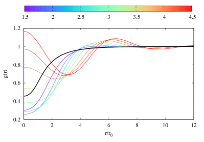
Figure 1: Pair distribution function $g(r)$ for the ground state of a three-dimensional Rydberg-dressed Bose gas for fixed interaction strength $U/E_{0}=2$ and for interaction ranges $R/r_{0}=1.5;2.0;2.5;3.0;3.5;4.0;4.3;4.5$, indicated by color. The thick black line shows $g(r)$ for $R/r_{0}=1$, the initial value before the quench.

We study quenches from weak to strong interactions. We keep $U$ fixed at $U_{0}=2E_{0}$, but switch $R(t)$ at $t=0$, from $R/r_{0}=1$ to $R/r_{0}=1.5;2.0;2.5;3.0;3.5;4.0;4.3;4.5$. Fig.1 shows the corresponding ground state pair density distributions $g(r)$. The oscillations in $g(r)$ become more pronounced as $R$ grows, and the range of correlations increases. Typically for the interaction (13), particles tend to cluster for larger $R$, eventually leading to a cluster solidCinti et al. (2010). This tendency to cluster is seen in the growth of $g(r)$ for small distance $r$ as we increase $R$.

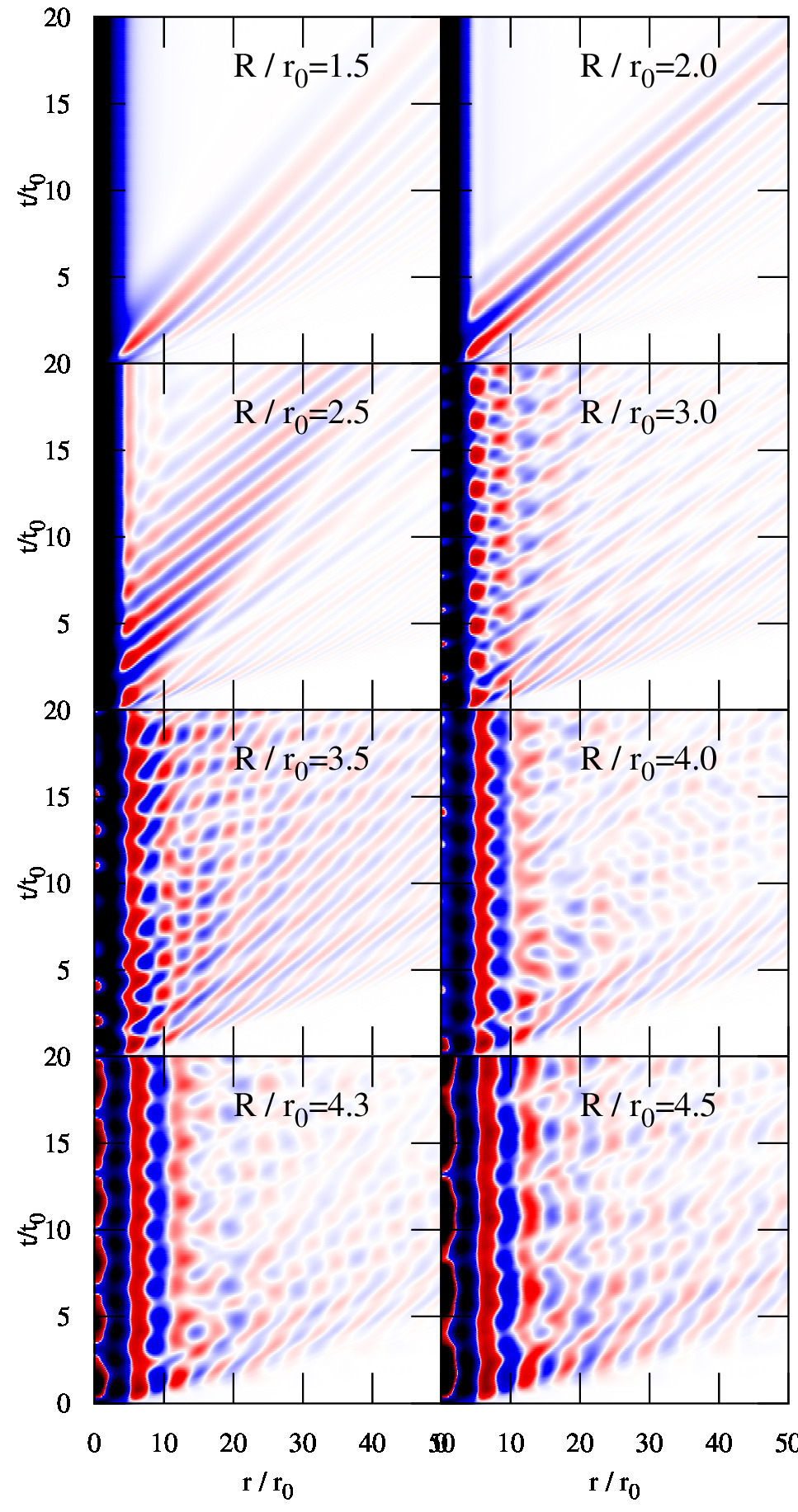
Figure 2: Pair distribution function $g(r,t)$ of a 3D Rydberg-dressed Bose gas after a quench from $R=1$ to $R=1.5;2.0;2.5;3.0;3.5;4.0;4.3;4.5$, with fixed $U=2$.

The time evolution of $g(r,t)$ after a quench from ${R/r_{0}=1}$ to the target values is shown in Fig. 2 as color maps, where the horizontal axis is the distance $r$ and the vertical axis is the time $t$. For small target values $R_{1}=1.5r_{0}$ and $2r_{0}$, the information about the quench of the pair interaction is spreading to larger distances $r$ as time evolves. We note that there is no “light cone” boundary. The light cone bound by Lieb and RobinsonLieb and Robinson (1972) applies only to discrete Hamiltonians, and was found for the Bose Hubbard model in Ref. Carleo et al., 2014 with tVMC. An effective light cone can appear if the group velocity $v_{g}$ of the elementary excitations has an upper bound $c$. Then a quench can excite two waves in opposite directions (conserving total momentum zero); the information about the quench would travel with $2c$, hence the response of $g(r,t)$ is expected to move with $2c$ to larger $r$. In lattice Hamiltonians there is a finite interval of quasi-momenta and thus $v_{g}$ must have a maximum, usually the sound velocity, with which information can spread. Here we have a continuous Hamiltonian, therefore there is no restriction on $v_{g}$. Indeed closer inspection reveals oscillation of $g(r,t)$ with very large wave numbers that travel very fast.

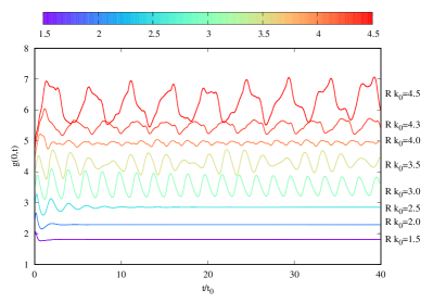
Figure 3: The pair distribution at $r=0$, $g(0,t)$, after a quench from $R_{0}/r_{0}=1$ to $R_{1}/r_{0}=1.5;2.0;2.5;3.0;3.5;4.0;4.3;4.5$, with fixed $U=2$. The curves are shifted with respect to each other for better visibility.

For small $R_{1}$, $g(r,t)$ quickly converges to an equilibrium distribution in an $r$-interval that grows with time, as the perturbation travels away to large $r$. The equilibrium is not the ground state $g(r)$ at the same $R_{1}$, which can be understood because the quench injects energy into the system. For example for the quench from $R_{0}=1r_{0}$ to $R_{1}=2r_{0}$, the energy jumps from $E=0.073E_{0}$ (the ground state energy before the quench) to $E=0.739E_{0}$ and then of course stays constant during the unitary time evolution; the ground state energy for $R_{1}=2r_{0}$, however, is $E_{g}=0.643E_{0}$. The question of thermalization will be investigated elsewhere.

When we quench the interaction to larger $R_{1}$, there is a qualitative change in $g(r,t)$: we observe long-lived oscillations for $R_{1}\geq 3r_{0}$ that do not decay within the time window shown in Fig.2. This can be seen for example for small $r$. In Fig. 3 we show $g(r,t)$ for $r=0$ for all target values $R_{1}$. The pair distribution function at $r=0$ is one way of obtaining the contact parameter Tan (2008); Werner and Castin (2012) which can be measured Wild et al. (2012). For $R_{1}\leq 2.5r_{0}$, $g(0,t)$ converges to a constant value, which lies slightly above the ground state $g(0)$.

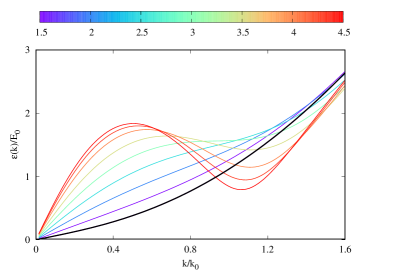
Figure 4: Bijl-Feynman spectrum $\varepsilon_{F}(k)$ of the ground state after a quench from $R=1$ to $R=1.5;2.0;2.5;3.0;3.5;4.0;4.3;4.5$, with fixed $U=2$. The thick black curve is $\varepsilon_{F}(k)$ before the quench, i.e. for $R=1$.

For $R_{1}\geq 3r_{0}$, $g(0,t)$ appears to keep oscillating indefinitely. Apart from $R_{1}=3r_{0}$, the oscillations clearly contain more than one frequency. The origin of this long-lived oscillation for small $r$ becomes apparent, when we invoke the picture of a quench generating two opposite excitations. In Fig. 4 we show the excitation spectrum $\varepsilon_{F}(k)$ for the initial $R_{0}$ before the quench (thick line) and the target values $R_{1}$ (colored lines), using the Bijl-Feynman approximationBijl (1940); Feynman and Cohen (1956), $\varepsilon_{F}(k)={\hbar^{2}k^{2}\over 2m\,S(k)}$. The Bijl-Feynman spectrum is calculated with the ground state static structure factor $S(k)$ obtained from a ground state HNC-EL/0 calculation with the respective value $R_{1}$. For small $R_{1}$, $\varepsilon_{F}(k)$ increases monotonously with wave number $k$. For $R_{1}=3r_{0}$, $\varepsilon_{F}(k)$ has a plateau with essentially zero slope around $k/k_{0}=1$, and for larger $R_{1}$, $\varepsilon_{F}(k)$ exhibits a maximum, called maxon, with energy $\hbar\omega_{m}$ and minimum, called roton, at energy $\hbar\omega_{r}$. A vanishing group velocity $v_{g}(k)={d\varepsilon_{F}(k)\over dk}$ implies a diverging density of state, leading to a high probability to excite excitatons with $v_{g}\approx 0$. Furthermore, the excitation pairs of opposite momenta produced by the quench do not propagate for $v_{g}=0$. For $R_{1}>3r_{0}$, roton pairs as well as maxon pairs with opposite momenta are generated. Since they do not propagate, the temporal oscillations for small distance $r$ become long-lived for $R_{1}\geq 3r_{0}$.

For $R_{1}=3r_{0}$, $g(0,t)$ oscillates with a single frequency because maxon and roton coincide at the inflection point of $\varepsilon_{F}(k)$. The frequency is twice the corresponding excitation energy (because the quench produces a pair of excitations). For $R_{1}>3r_{0}$, $g(0,t)$ oscillates with two frequencies, given by twice the roton and twice the maxon frequency. In order to confirm this quantitatively, we show the power spectra $P(\omega)$ of $g(0,t)$ in Fig. 5, as functions of $\omega/2$. Each $P(\omega)$ is shifted in proportion to $R_{1}$ for better visibility. For $R_{1}<3r_{0}$, the power spectra are broad. At $R_{1}=3r_{0}$ a single peak appears, corresponding to the single frequency oscillations seen in Fig.3. For $R_{1}>3r_{0}$, $P(\omega)$ has two peaks of varying relative spectral weight: at twice the roton frequency $2\omega_{r}$ and at twice the maxon frequency $2\omega_{m}$ (the combination $\omega_{r}+\omega_{m}$ would have finite momentum and cannot be excited in this simple picture by a translationally invariant perturbation such as an interaction quench). The small ringing oscillations are artifacts from the Fourier transformation of a finite time window $[0,40t_{0}]$.

However, $\omega_{r}$ and $\omega_{m}$, which are indicated by stars in Fig.5 for the respective $R_{1}$, do not match perfectly with the peaks of $P(\omega)$. The picture of an interaction quench exciting two elementary excitations with opposite momenta is only approximately valid. A quench from $R_{0}/r_{0}=1$ to e.g. $R_{1}/r_{0}=4.5$ is a highly nonlinear process which tends to shift the lower-frequency below $2\omega_{r}$ and the higher-frequency peak above $2\omega_{m}$. The effect of nonlinearity is demonstrated in the inset, where the power spectrum $P(\omega)$ for the quench $r_{0}\to 4.5r_{0}$ shown in the main figure (red) is compared with $P(\omega)$ for a much weaker quench $4r_{0}\to 4.5r_{0}$ (black). In the latter case, the power spectrum has a peak much closer to $2\omega_{r}$; the excitation of two maxons is suppressed.

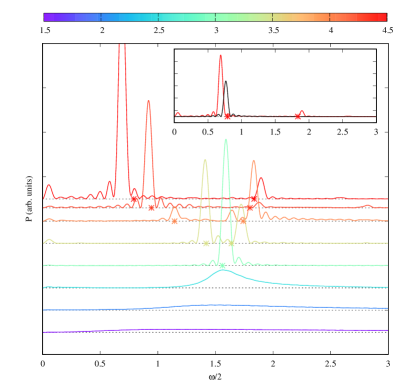
Figure 5: Power spectrum $P(\omega)$ of $g(0,t)$ shown in Fig. 3, after a quench from $R=1$ to $R=1.5;2.0;2.5;3.0;3.5;4.0;4.3;4.5$, with fixed $U=2$. The curves are shifted with respect to each other for better visibility. The stars on the base line indicate the energies of the roton and the maxon after the quench, if present. The inset compares $P(\omega)$ after a quench to $R_{1}=4.5$ starting from $R=1$ (red) with a quench starting from $R=4$ (black).

III.2 Comparison with tVMC

We compare tHNC results for the quench dynamics with corresponding results obtained with time-dependent variational Monte Carlo (tVMC) simulations Carleo et al. (2012). Details about our implementation of tVMC can be found in the appendix and in Ref.Gartner et al., 2022. We use the same Jastrow ansatz (3) as in the tHNC method. However, tVMC does not require an approximation for $g_{3}$ nor does tVMC need to use approximations for the elementary diagrams, because all integrations over the $N$-body configuration space are performed by brute force Monte Carlo sampling. The price is, of course, a much higher computational cost. Therefore we have restricted the comparisons with tVMC to one and two dimensions.

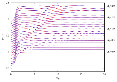
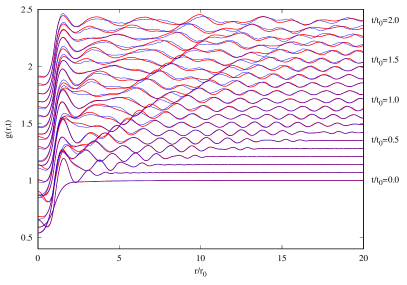
Figure 6: Comparison of the pair distribution function $g(r,t)$ for a Bose gas in 1D between tHNC (red) and tVMC (blue). The interaction is the square well potential (14), quenched from initial strength $U=2E_{0}$ to a strength $U=4E_{0}$ (left panel) and $U=8E_{0}$ (right panel), respectively. For better visibility $g(r,t)$ is shifted in proportion to time, indicated on the right margin.

III.2.1 Comparison in 1D

For the 1D comparison we use a square well potential

$$v(r,t) =U(t)\Theta[R(t)-r]$$ (14)

characterized by strength $U(t)$ and range $R(t)$. The length and energy units are $r_{0}=\rho^{-1}$ and $E_{0}={\hbar^{2}\over 2mr_{0}^{2}}$. In the tVMC simulations we use $N=100$ particles, corresponding to a simulation box size $L=100r_{0}$. We can thus calculate $g(r,t)$ up to a maximal distance $r=50r_{0}$; when fluctuations reach this maximal distance, spurious reflections appear due to the periodic boundary conditions. We restrict our comparisons of $g(r,t)$ with tHNC to times $t$ before these reflections become noticeable. We approximate the Jastrow pair-correlation $u(r)$ with $P=400$ splines, corresponding to $P$ complex variational parameters $\alpha_{i}(t)$, as explained in the appendix. The time propagation is performed with a time step of $\Delta t=2\cdot 10^{-4}\,t_{0}$, and ${N_{\text{MC}}=1250}$ uncorrelated samples are used for calculating the expectation values required for time propagation. The results are converged with respect to the spatial and temporal numerical resolution because we see no changes upon increasing $P$ or decreasing $\Delta t$.

In Fig. 6 we compare $g(r,t)$ after a quench. The interaction range is fixed at $R/r_{0}=1$ and the interaction strength jumps from $U=2E_{0}$ to a target value $U=4E_{0}$ (top panel) and to $U=8E_{0}$ (bottom panel). We show $g(r,t)$ at times $t/t_{0}=0.0;0.1;0.2;\dots;2.0$. For the weaker first quench, the agreement between tHNC (red) and tVMC (blue) is excellent, because the target interaction is weak enough that neglecting elementary diagrams and the Kirkwood superposition approximation (7) for the three body distribution $g_{3}$ are still good approximations. For the stronger quench to a target value $U=8E_{0}$ the tHNC and tVMC results for $g(r,t)$ do not match perfectly anymore. For strong interaction, the effect of elementary diagrams or the three body distribution or both becomes more important. But overall, the agreement is still remarkably good; for example, both frequency and phase shift of the oscillations in $g(r,t)$ are the same. We conclude that tHNC works quite well compared to tVMC in 1D, despite the approximations that we use in our simple implementation of tHNC. Of course, for strong interactions, even tVMC with pair correlations is not sufficient for quantitative predictions of the dynamics in 1D and a better variational ansatz than (3) should be used.

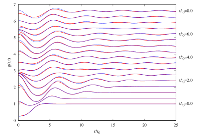
Figure 7: Comparison of the pair distribution function $g(r,t)$ for a Bose gas in 2D between tHNC (red) and tVMC (blue). The interaction is the Rydberg potential (13), quenched from initial range $R=2r_{0}$ to $R=4r_{0}$. For better visibility $g(r,t)$ is shifted in proportion to time, indicated on the right margin.

III.2.2 Comparison in 2D

For the 2D comparison we use the Rydberg-dressed interaction (13) from the 3D studies in the previous section III.1. We use the 2D version of the units introduced above for 3D, see also Seydi et al. (2020): wave numbers are in units of $k_{0}=(4\pi\rho)^{1/2}$, and again length in units of $r_{0}=1/k_{0}$, energy in units of $E_{0}={\hbar^{2}k_{0}^{2}\over 2m}$, and time in units of $t_{0}={\hbar\over E_{0}}$. In the tVMC simulations we use $N=900$ particles, corresponding to a simulation box size $L=106.347r_{0}$. ${P=300}$ variational parameters, a time step of ${\Delta t=2\cdot 10^{-4}\,t_{0}}$ and ${N_{\text{MC}}=1250}$ samples are used. Again, we compare only up to times before effects of the periodic boundaries contaminate the dynamics of $g(r,t)$.

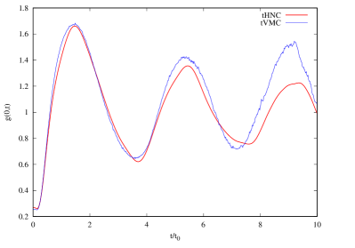
Figure 8: For the quench in Fig. 7, we compare the roton-induced oscillation of $g(r,t)$ for $r=0$ between tHNC (red) and tVMC (blue).

Following the quench procedure in our 3D tHNC calculations above, we keep $U$ fixed at $U_{0}=2E_{0}$, and switch $R(t)$ from $R/r_{0}=2$, where excitations from the ground state are monotonous, to $R/r_{0}=4$, where the excitation spectrum exhibits rotons. Fig. 7 compares the tHNC result (red) and tVMC result (blue) for $g(r,t)$ after the quench. As in 1D, we find good agreement between tHNC and tVMC before spurious oscillations due to the period boundary conditions in tVMC appear for later times (not shown). As expected from our 3D calculations, the creation of pairs of rotons leads to persistent oscillations in $g(r,t)$ for small $r$. The amplitude, however, becomes smaller in the tHNC results, as can be seen in Fig.8, which compares $g(r,t)$ for $r=0$. Again, the differences between tHNC and tVMC are due to the approximations made in our present implementation of tHNC. When $g(0,t)$ becomes large, particles tend to cluster together, and we expect that particularly the Kirkwood superposition form (7) for $g_{3}$ is a poor approximation.

IV Discussion

We present a new method for studying quantum many-body dynamics far from equilibrium, the time-dependent generalization of the hypernetted-chain Euler-Lagrange method, tHNC, which is non-perturbative and goes beyond the mean field paradigm. We demonstrate this variational method in a study of the interaction quench dynamics of a homogeneous Rydberg-dressed Bose gas. A sudden strong change of the effective Rydberg interaction leads to a strong response of the pair distribution function $g(r,t)$, which is the quantity we are interested in in this work. In an interaction quench, the Hamiltonian becomes time-dependent but is still translationally invariant. The systems stay homogeneous and only pair quantities like $g(r,t)$ carry the dynamics (we assume there is no spontaneous breaking of translation invariance).

We derived the Euler-Lagrange equations of motion for $g(r,t)$ for the simplest case, where elementary diagrams in the HNC relations are omitted, and only pair correlations $u_{2}$ are taken into account in the variational ansatz for the many-body wave function (Jastrow-Feenberg ansatz). This simple version is long known in various formulations for ground state calculations Campbell (1978); Lantto and Siemens (1977) and is sufficient for not too strongly correlated Bose systems (but not sufficient for quantitative predictions of energy and structure of e.g. liquid ⁴He).

The dynamics of the pair distribution $g(r,t)$ of a Rydberg-dressed 3D gas is similar to results of previous tVMC studies of bosons on a deep 2D lattice, described by the Bose-Hubbard model Carleo et al. (2014), and bosons in 1D Carleo et al. (2017). After a weak quench a “wave” travels to larger distances. Unlike for the dynamics on a lattice, we observe no light-cone restriction for the speed of propagation since our group velocity is not bounded from above. Ripples of very high wave number indeed move very fast towards larger distances. We stress that these waves are not density fluctuations (which would break translation symmetry) but fluctuations of the pair density.

There is a qualitative change in the behavior of $g(r,t)$ for a strong quench. If the interaction after the quench is strong enough that a linear response calculation predicts a roton excitation, i.e. a non-monotonous dispersion relation, $g(r,t)$ exhibits long-lasting oscillations for small $r$ that do not decay within our calculation time windows. This can be readily understood as the creation of a pair of rotons with opposite momentum (total momentum is conserved by an interaction quench). The group velocity of rotons vanishes, therefore the oscillations of $g(r,t)$ due to rotons do not propagate to larger $r$; furthermore the density of states for rotons diverges, therefore exciting roton pairs is very efficient. The argument is equally valid for the maxon, i.e. the local maximum of the dispersion relation. Finally, since the quench creates a pair of rotons or maxons (a roton-maxon pair would violate momentum conservation), the oscillations have twice the roton or maxon frequencies. Indeed for these strong quenches the power spectra have peaks at almost these frequencies, and not much strength at other frequencies. The peaks are slightly off from twice the roton or maxon frequency due to nonlinear effects, which we confirmed by smaller, hence more linear-response-like, jumps in the interaction quench.

Apart from the Jastrow-Feenberg ansatz with pair correlations, the tHNC equations contain two approximations, the already mentioned omission of elementary diagrams, and an approximation for the three-body distribution function $g_{3}({\bf r}_{1},{\bf r}_{2},{\bf r}_{3})$, where we chose the straightforward Kirkwood superposition approximation. In order to assess these two approximations, we performed tVMC simulations of interaction quenches. We restricted ourselves to one and two dimensions due to the high computational cost of tVMC. Overall we see good agreement between tHNC and tVMC. In 1D we compared for two different quenches, finding excellent agreement for the weaker quench. As the interaction strength after the quench increases the agreement worsens somewhat, but all the main features such as the roton-induced oscillations in the 2D comparison are captured already by tHNC. For very strong interaction, we would need to (i) incorporate elementary diagrams – this can be done approximately in the same way as in ground state HNC-EL calculations; (ii) improve upon the Kirkwood superposition approximation (e.g. use the systematic Abe expansionFeenberg (1969)) or use other approximations like the convolution approximation Hansen and McDonald (1976). However, note that for strong interactions triplet correlations $u_{3}$ should be included in the variational ansatz, both for tHNC and tVMC.

Like the ground state HNC-EL method, tHNC can be generalized to inhomogeneous and/or anisotropic systems. The latter is important for dipolar Bose gases, while most quantum gas experiments are in harmonic or optical traps rather than in box traps, and thus require an inhomogeneous description; even in case of an interaction quench of a homogeneous Bose gas, the quench may trigger spontaneous breaking of translational invariance. The diagrammatic summations used in the ground state HNC-EL method have been generalized to off-diagonal properties like the 1-body density matrix to study off-diagonal long-range order, i.e. the Bose-Einstein condensed fraction Manousakis et al. (1985). We will generalize this to the time-dependent case. Further down the road, we plan to include three body correlations $u_{3}$ at least approximately, known to improve ground states of highly correlated systemsKrotscheck (1986). This opens a new scattering channel, where an interaction quench can generate excitation triplets, not just pairs, with total momentum zero. In case of quenches to rotons, the oscillation pattern of $g(r,t)$ will be more complex because its power spectrum can contain frequencies corresponding to the energies of three rotons. We are also generalizing tHNC to anisotropic interaction in order to study the non-equilibrium dynamics of dipolar quantum gases. Studying the long-time dynamics after a nonlinear perturbation, such as a strong interaction quench, requires numerical stability for very long times, which is challenging for nonlinear problems like solving the tHNC equations or the equations of motion of tVMC. A small time step is required to achieve long-time stability for both tHNC and tVMC. However, tHNC is computationally very cheap and calculations of the long-time dynamics are feasible. In order to delay artifacts from reflections at domain boundaries, either the spatial domain must be chosen very large, or absorbing boundary conditions are implemented.

Appendix A Derivation of the tHNC equation

We derive the tHNC equation of motion (10) using the time-dependent variational principle $\delta\mathcal{S}=0$, where $\mathcal{S}$ is the action. All quantities depend on time $t$, but for brevity we omit the $t$ argument in what follows.

The action is given by eqns. (4) and (5) as

$$\mathcal{S}=\mathcal{S}_{g}+\mathcal{S}_{2}+\mathcal{S}_{3}$$

with

$$\mathcal{S}_{g} ={\rho\over 2}\int\limits_{t_{0}}^{t}\!dt^{\prime}\!\!\int\!\!d^{d}r\Big{[}v(r)-{\hbar^{2}\over 4m}\Delta u(r)\Big{]}g(r),$$

$$\mathcal{S}_{2} ={\hbar\over 2}\int\limits_{t_{0}}^{t}\!dt^{\prime}\!\!\int\!\!d^{d}r\,\dot{\varphi}(r)\,g(r)+{\hbar^{2}\over 2m}\rho\!\int\limits_{t_{0}}^{t}\!dt^{\prime}\!\!\int\!\!d^{d}r\,{\bf v}({\bf r})^{2}g(r),$$

$$\mathcal{S}_{3} ={\hbar^{2}\over 2m}\rho^{2}\!\int\limits_{t_{0}}^{t}\!dt^{\prime}\!\!\int\!\!d^{d}rd^{d}r^{\prime}\,{\bf v}({\bf r})\cdot{\bf v}({\bf r}^{\prime})\,g_{3}(r,r^{\prime},|{\bf r}-{\bf r}^{\prime}|),$$

where ${{\bf v}({\bf r})\equiv\nabla\varphi(r)}$.

The Euler-Lagrange equations (8) and (9) require the functional differentiation of $\mathcal{S}_{g}$, $\mathcal{S}_{2}$, and $\mathcal{S}_{3}$ with respect to $g(r)$ and $\varphi(r)$. Apart from time integration, $\mathcal{S}_{g}$ is the same expression as the energy expectation value of the ground state HNC-EL method. It does not depend on $\varphi(r)$ and the differentiation with respect to $g(r)$, using the HNC relation (6), can be found in reviews on HNC-EL, e.g. Ref. Polls and Mazzanti, 2002. The derivates of $\mathcal{S}_{2}$ are

$${\delta\mathcal{S}_{2}\over\delta g(r)} ={\hbar\over 2}\dot{\varphi}(r)+{\hbar^{2}\over 2m}{\bf v}({\bf r})^{2},$$

$${\delta\mathcal{S}_{2}\over\delta\varphi(r)} =-{\hbar\over 2}\dot{g}(r)-{\hbar^{2}\over 2m}\nabla\left[g(r)\cdot{\bf v}({\bf r})\right].$$

In $\mathcal{S}_{3}$ we employ the Kirkwood superposition approximation (7)

$$\mathcal{S}_{3} ={\hbar^{2}\over 2m}\rho^{2}\!\int\limits_{t_{0}}^{t}\!dt^{\prime}\!\!\int\!\!d^{d}rd^{d}r^{\prime}\,{\bf f}({\bf r})\cdot{\bf f}({\bf r}^{\prime})\,g(|{\bf r}-{\bf r}^{\prime}|)$$

with ${\bf f}({\bf r})\equiv g(r)\,{\bf v}({\bf r})$. The derivatives are

$${\delta\mathcal{S}_{3}\over\delta g(r)} ={\hbar^{2}\over m}{\bf v}({\bf r})\cdot\nabla\gamma(r)+{1\over 2}\beta(r),$$

$${\delta\mathcal{S}_{3}\over\delta\varphi(r)} =-{\hbar^{2}\over m}\nabla\left[g(r)\cdot\nabla\gamma(r)\right].$$

where $\beta(r)$ and $\nabla\gamma(r)$ are defined in eqns.(11) and (12), respectively.

Putting everything together, equation (8) becomes, after multiplying by 2,

$$0 =-{1\over\sqrt{g(r)}}{\hbar^{2}\over m}\nabla^{2}\sqrt{g(r)}+v(r)+w_{I}(r)$$

$$+\hbar\dot{\varphi}(r)+{\hbar^{2}\over m}[\nabla\varphi(r)]^{2}$$

$$+2{\hbar^{2}\over m}\nabla\varphi(r)\cdot\nabla\gamma(r)+\beta(r).$$ (15)

If we keep only the first line of the equation, we recover the ground state HNC-EL equation (where $\varphi=0$, of course). The induced potential $w_{I}(r)$ describing phonon-mediated interactions can be found in Ref. Polls and Mazzanti, 2002. Equation (9) becomes

$$0 =-{1\over 2}\hbar\dot{g}(r)-{\hbar^{2}\over m}\nabla\left[g(r)\cdot\nabla(\varphi(r)+\gamma(r)\right].$$ (16)

When we multiply eq.(15) with $\sqrt{g(r)}$ and eq.(16) with ${i/\sqrt{g(r)}}$, add the two equations, and multiply the resulting equation with $e^{i\varphi(r)}$, we obtain the final form (10) of the tHNC equation for the effective pair wave function $\psi(r)=\sqrt{g(r)}e^{i\varphi(r)}$ that we use for the numerical solution.

Appendix B tVMC method

In tVMCCarleo et al. (2012, 2014, 2017), we use the same Jastrow-Feenberg ansatz (3) as in tHNC, and describe the time dependence via a set of $P$ complex variational parameters ${\alpha(t)=\{\alpha_{1}(t),\alpha_{2}(t),\ldots,\alpha_{P}(t)\}}$, which are coupled to local operators ${\mathcal{O}_{m}({\bf r}_{1},\ldots,{\bf r}_{N})}$. In our implementation (more details can be found in Gartner et al. (2022)), these local operators are represented by third order B-splines $B_{m}(r)$ centered on a uniform grid in the interval $[0,L/2]$, and are given by ${\mathcal{O}_{m}({\bf r}_{1},\ldots,{\bf r}_{N})=\sum_{k<l}B_{m}(r_{kl})}$. The real and imaginary part of the pair correlation function $u_{2}(r)$ can then be written as

$$u(r) =\sum_{m}^{P}B_{m}(r)\alpha_{m}^{R}(t) \varphi(r) =\sum_{m}^{P}B_{m}(r)\alpha_{m}^{I}(t),$$

where $\alpha_{m}^{R}$ and $\alpha_{m}^{I}$ are the real and imaginary part of $\alpha_{m}$. The time evolution of the variational wavefunction is obtained by solving the coupled system of equations (see Carleo et al. (2012))

$$i\sum_{n}S_{mn}\dot{\alpha}_{n}=\langle\mathcal{E}\mathcal{O}_{m}\rangle-\langle\mathcal{E}\rangle\langle\mathcal{O}_{m}\rangle,$$

with the correlation matrix ${S_{mn}=\langle\mathcal{O}_{m}\mathcal{O}_{n}\rangle-\langle\mathcal{O}_{m}\rangle\langle\mathcal{O}_{n}\rangle}$ and the local energy ${\mathcal{E}=\frac{H|\Phi\rangle}{|\Phi\rangle}}$. The expectation values $\langle\ldots\rangle$ are estimated using Monte Carlo integration by sampling from the trial wavefunction ${\Phi({\bf r}_{1},\ldots,{\bf r}_{N},t)=\exp\left(\sum_{k<l}u_{2}(r_{kl},t)\right)}$. Because of the translational invariance of the studied system we do not need to take into account a one-body part $u_{1}(r,t)$ in the wavefunction, unlike in Ref. Gartner et al. (2022) where the dynamics of a Bose gas in a 1D optical lattice has been simulated.

References

- Schreiber et al. (2015) M. Schreiber, S. S. Hodgman, P. Bordia, H. P. Lüschen, M. H. Fischer, R. Vosk, E. Altman, U. Schneider, and I. Bloch, Science 349, 842 (2015), publisher: American Association for the Advancement of Science.
- Heyl et al. (2013) M. Heyl, A. Polkovnikov, and S. Kehrein, Phys. Rev. Lett. 110, 135704 (2013), publisher: American Physical Society.
- Jurcevic et al. (2017) P. Jurcevic, H. Shen, P. Hauke, C. Maier, T. Brydges, C. Hempel, B. Lanyon, M. Heyl, R. Blatt, and C. Roos, Phys. Rev. Lett. 119, 080501 (2017), publisher: American Physical Society.
- Zhang et al. (2017) J. Zhang, G. Pagano, P. W. Hess, A. Kyprianidis, P. Becker, H. Kaplan, A. V. Gorshkov, Z.-X. Gong, and C. Monroe, Nature 551, 601 (2017), number: 7682 Publisher: Nature Publishing Group.
- Mistakidis et al. (2019) S. Mistakidis, G. Katsimiga, G. Koutentakis, T. Busch, and P. Schmelcher, Phys. Rev. Lett. 122, 183001 (2019), publisher: American Physical Society.
- Karl and Gasenzer (2017) M. Karl and T. Gasenzer, New J. Phys. 19, 093014 (2017), publisher: IOP Publishing.
- Vidal (2004) G. Vidal, Physical Review Letters 93, 040502 (2004).
- Aoki et al. (2014) H. Aoki, N. Tsuji, M. Eckstein, M. Kollar, T. Oka, and P. Werner, Reviews of Modern Physics 86, 779 (2014).
- White (1992) S. R. White, Physical Review Letters 69, 2863 (1992).
- Feiguin and White (2005) A. E. Feiguin and S. R. White, Physical Review B 72, 020404 (2005).
- Schollwöck (2005) U. Schollwöck, Reviews of Modern Physics 77, 259 (2005).
- Verstraete and Cirac (2010) F. Verstraete and J. I. Cirac, Physical Review Letters 104, 190405 (2010).
- Lode et al. (2020) A. U. J. Lode, C. Lévêque, L. B. Madsen, A. I. Streltsov, and O. E. Alon, Reviews of Modern Physics 92, 011001 (2020).
- Krotscheck (1986) E. Krotscheck, Phys. Rev. B 33, 3158 (1986).
- Krotscheck (2002) E. Krotscheck, in Introduction to Modern Methods of Quantum Many–Body Theory and their Applications, Advances in Quantum Many–Body Theory, Vol. 7, edited by A. Fabrocini, S. Fantoni, and E. Krotscheck (World Scientific, Singapore, 2002) pp. 267–330.
- Polls and Mazzanti (2002) A. Polls and F. Mazzanti, in Introduction to Modern Methods of Quantum Many-Body Theory and Their Applications, Series on Advances in Quantum Many Body Theory Vol.7, edited by A. Fabrocini, S. Fantoni, and E. Krotscheck (World Scientific, 2002) p. 49.
- Campbell et al. (2015) C. E. Campbell, E. Krotscheck, and T. Lichtenegger, Physical Review B 91, 184510 (2015).
- Carleo et al. (2012) G. Carleo, F. Becca, M. Schiró, and M. Fabrizio, Scientific Reports 2, 243 (2012).
- Carleo et al. (2014) G. Carleo, F. Becca, L. Sanchez-Palencia, S. Sorella, and M. Fabrizio, Physical Review A 89, 031602 (2014).
- Carleo et al. (2017) G. Carleo, L. Cevolani, L. Sanchez-Palencia, and M. Holzmann, Physical Review X 7, 031026 (2017).
- Navon et al. (2021) N. Navon, R. P. Smith, and Z. Hadzibabic, Nat. Phys. 17, 1334 (2021), number: 12 Publisher: Nature Publishing Group.
- Dawid et al. (2022) A. Dawid, J. Arnold, B. Requena, A. Gresch, M. Płodzień, K. Donatella, K. Nicoli, P. Stornati, R. Koch, M. Büttner, R. Okuła, G. Muñoz-Gil, R. A. Vargas-Hernández, A. Cervera-Lierta, J. Carrasquilla, V. Dunjko, M. Gabrié, P. Huembeli, E. van Nieuwenburg, F. Vicentini, L. Wang, S. J. Wetzel, G. Carleo, E. Greplová, R. Krems, F. Marquardt, M. Tomza, M. Lewenstein, and A. Dauphin, “Modern applications of machine learning in quantum sciences,” (2022).
- Hansen and McDonald (1976) J. P. Hansen and I. R. McDonald, Theory of Simple Liquids (Academic Press, New York, 1976).
- Saarela (2002) M. Saarela, in Introduction to Modern Methods of Quantum Many-Body Theory and Their Applications, Series on Advances in Quantum Many Body Theory Vol.7, edited by A. Fabrocini, S. Fantoni, and E. Krotscheck (World Scientific, 2002) p. 205.
- Stapelfeldt and Seideman (2003) H. Stapelfeldt and T. Seideman, Rev. Mod. Phys. 75, 543 (2003).
- Chatterley et al. (2020) A. S. Chatterley, L. Christiansen, C. A. Schouder, A. V. Jørgensen, B. Shepperson, I. N. Cherepanov, G. Bighin, R. E. Zillich, M. Lemeshko, and H. Stapelfeldt, Phys. Rev. Lett. 125, 013001 (2020), publisher: American Physical Society.
- Fechner et al. (2018) M. Fechner, A. Sukhov, L. Chotorlishvili, C. Kenel, J. Berakdar, and N. A. Spaldin, Phys. Rev. Mater. 2, 064401 (2018).
- Tulzer et al. (2020) G. Tulzer, M. Hoffmann, and R. E. Zillich, Phys. Rev. B 102, 125131 (2020), publisher: American Physical Society.
- Fletcher et al. (2017) R. J. Fletcher, R. Lopes, J. Man, N. Navon, R. P. Smith, M. W. Zwierlein, and Z. Hadzibabic, Science 355, 377 (2017), publisher: American Association for the Advancement of Science.
- Villa et al. (2021) L. Villa, S. J. Thomson, and L. Sanchez-Palencia, Phys. Rev. A 104, L021301 (2021), publisher: American Physical Society.
- Feenberg (1969) E. Feenberg, Theory of Quantum Fluids (Academic Press, 1969).
- Chin (2005) S. A. Chin, Phys. Rev. E 71, 016703 (2005).
- Pohl et al. (2010) T. Pohl, E. Demler, and M. D. Lukin, Phys. Rev. Lett. 104, 043002 (2010), publisher: American Physical Society.
- Cinti et al. (2010) F. Cinti, P. Jain, M. Boninsegni, A. Micheli, P. Zoller, and G. Pupillo, Phys. Rev. Lett. 105, 135301 (2010), publisher: American Physical Society.
- Henkel et al. (2010) N. Henkel, R. Nath, and T. Pohl, Phys. Rev. Lett. 104, 195302 (2010), publisher: American Physical Society.
- Seydi et al. (2020) I. Seydi, S. H. Abedinpour, R. E. Zillich, R. Asgari, and B. Tanatar, Phys. Rev. A 101, 013628 (2020), publisher: American Physical Society.
- McCormack et al. (2020) G. McCormack, R. Nath, and W. Li, Phys. Rev. A 102, 023319 (2020), publisher: American Physical Society.
- Natu et al. (2014) S. S. Natu, L. Campanello, and S. Das Sarma, Phys. Rev. A 90, 043617 (2014), publisher: American Physical Society.
- Lieb and Robinson (1972) E. H. Lieb and D. W. Robinson, Commun.Math. Phys. 28, 251 (1972).
- Tan (2008) S. Tan, Annals of Physics 323, 2952 (2008).
- Werner and Castin (2012) F. Werner and Y. Castin, Phys. Rev. A 86, 053633 (2012), publisher: American Physical Society.
- Wild et al. (2012) R. J. Wild, P. Makotyn, J. M. Pino, E. A. Cornell, and D. S. Jin, Phys. Rev. Lett. 108, 145305 (2012), publisher: American Physical Society.
- Bijl (1940) A. Bijl, Physica 7, 869 (1940).
- Feynman and Cohen (1956) R. P. Feynman and M. Cohen, Physical Review 102, 1189 (1956).
- Gartner et al. (2022) M. Gartner, F. Mazzanti, and R. E. Zillich, SciPost Phys. 13, 025 (2022).
- Campbell (1978) C. E. Campbell, in Progress in Liquid Physics, edited by C. A. Croxton (John Wiley & Sons, Ltd., 1978) Chap. 6, pp. 213–308.
- Lantto and Siemens (1977) L. J. Lantto and P. J. Siemens, Phys. Lett. B 68, 308 (1977).
- Manousakis et al. (1985) E. Manousakis, V. R. Pandharipande, and Q. N. Usmani, Phys. Rev. B 31, 7022 (1985), publisher: American Physical Society.