Simplification of Forest Classifiers and Regressors by Sharing Branching Conditions

Abstract

We study the problem of sharing as many branching conditions of a given forest classifier or regressor as possible while keeping classification performance. As a constraint for preventing from accuracy degradation, we first consider the one that the decision paths of all the given feature vectors must not change. For a branching condition that a value of a certain feature is at most a given threshold, the set of values satisfying such constraint can be represented as an interval. Thus, the problem is reduced to the problem of finding the minimum set intersecting all the constraint-satisfying intervals for each set of branching conditions on the same feature. We propose an algorithm for the original problem using an algorithm solving this problem efficiently. The constraint is relaxed later to promote further sharing of branching conditions by allowing decision path change of a certain ratio of the given feature vectors or allowing a certain number of non-intersected constraint-satisfying intervals. We also extended our algorithm for both the relaxations. The effectiveness of our method is demonstrated through comprehensive experiments using 21 datasets (13 classification and 8 regression datasets in UCI machine learning repository) and 4 classifiers/regressors (random forest, extremely randomized trees, AdaBoost and gradient boosting).

Keywords: simplification, tree ensemble, optimization, braching condition sharing, forest classifiers and regressors

1 Introduction

Edge computing is a key for realization of real time and low loading intelligent data processing. Highly accurate compact classifiers or regressors are necessary for edge computing devices. To produce compact models, researches by various approaches have been done (Murshed et al., 2021) including directly learning compact models (Gupta et al., 2017; Kumar et al., 2017) and post processing like quantization and compression.

Ensemble classifiers and regressors are very popular predictors due to their good accuracy and robustness. The most frequently used ensembles are tree ensembles that include random forests (Breiman, 2001), extremely randomized trees (Geurts et al., 2006), AdaBoost (Freund and Schapire, 1997) gradient boosted regression trees (Friedman, 2000), and XGBoost (Chen and Guestrin, 2016).

In this paper, we study simplification of tree ensembles for post-processing compression. As such simplification method, pruning (Kulkarni and Sinha, 2012) has been studied for more than three decades. Most existing pruning techniques reduce the number of branching nodes or trees. We, however, consider post-compression methods that simplify a given tree ensemble by sharing branching conditions without changing the structure of the tree ensemble. Branching condition sharing is corresponding to comparator sharing which contributes to compact hardware implementation of tree ensemble predictors (JINGUJI et al., 2018; Ikeda et al., 2020). Though comparator sharing by threshold clustering has been already studied by JINGUJI et al. (2018) before our research, we pursue a more sophisticated method than simply integrating similar threshold values.

Firstly, we formalize our simplification problem as the problem of minimizing the number of distinct branching conditions in a tree ensemble by condition sharing under the constraint that any decision path of the given feature vectors must not be changed. We consider the case that all the features are numerical and every branching condition is the condition that the value of a certain feature is at most a certain threshold $\theta$. Then, the range of $\theta$ that satisfies the above constraint becomes some interval $[\ell,u)$, and the problem can be reduced to each feature’s problem of obtaining a minimum set that intersects all the range intervals of its thresholds. We propose Algorithm Min_IntSet for this reduced problem and prove its correctness. We also develop Algorithm Min_DBN for our original problem using Min_IntSet to solve the reduced problem for each feature.

To promote further sharing of branching conditions, in addition to simplely using of bootstrap training samples per tree, we propose two extended problems by relaxation of the restriction. One is relaxation by allowing the existence of feature vectors whose decision paths change. We introduce a parameter $\sigma$ called “path changeable rate” and allow $100\sigma$% feature vectors passing through each node to change. The other is relaxation by allowing the existence of non-intersecting intervals in the reduced problem. We introduce a parameter $c$, the number of allowable exceptions, and allow at most $c$ intervals that are not intersected by the solution set in the reduced problem. For both extended problems, we provide solution algorithms and their time and space complexities.

The effectiveness of our algorithm Min_DBN and its extensions were demonstrated using 13 classification and 8 regression datasets in the UCI machine learning repository (Dua and Karra Taniskidou, 2017), and four major tree ensembles, random forest (RF), extremely randomized trees (ERT), AdaBoost (ABoost) and gradient boosting (GBoost), whose implementations are provided by scikit-learn python library (Pedregosa et al., 2011). For each dataset, we conducted a 5-fold cross validation, and four folds were used to generate the tree ensemble classifiers and regressors, to which our simplification algorithms were applied. The remaining one fold was used to check accuracy degradation. Medians of the reduced size ratios among all the 21 datasets are 18.1%, 2.1%, 45.9%, and 85.9% for RF, ERT, ABoost, and GBoost, respectively, while all the accuracy degradations are within 1% except one dataset for ERT. Among our two extensions, the method allowing exceptional intervals performs better than the method allowing exceptional feature vectors in terms of size ratio and accuracy degradation, though the computational cost of the former method is heavier than that of the latter method. As for the comparison with the k-means clustering-based method, the method allowing exceptional intervals found more accurate pareto optimal predictors in our experiment using systematically selected parameters.

1.1 Related Work

Pruning of tree classifiers and regressors is a very popular technique as a countermeasure of overfitting to training data (Esposito et al., 1997). Pruning is a kind of simplification of tree classifiers and regressors which reduces the number of nodes by replacing subtrees with leaves. Various pruning methods have been developed around 30 years ago (Quinlan, 1987; Niblett and Bratko, 1987; Breiman et al., 1984; Cestnik and Bratko, 1991; Mingers, 1989; Bohanec and Bratko, 1994). In the pruning of tree ensembles, in addition to directly applying pruning methods for a tree to each component tree (Windeatt and Ardeshir, 2001), node reduction considering prediction and accuracy of the whole ensemble classifier was developed; node importance-based pruning (Jiang et al., ) and the pruning using 0-1 integer programming treating both error and computational cost (Nan et al., 2016). The reduction of component trees was also realized by maximizing the diversity of component trees (Zhang et al., 2006) or minimizing the sum of voting integer weights for component trees without changing predictions of given feature vectors (Maekawa et al., 2020). The minimum single trees that are equivalent to given tree ensembles were reported to become smaller than the original tree ensembles without accuracy degradation by applying pruning that is based on given feature vectors to the equivalent single trees (Vidal and Schiffer, 2020).

Any simplification method for tree ensembles simplifies the input space partition of a given tree ensemble. As a direct simplification of the partition, reduction of the partitioned regions was done by the Bayesian model selection approach (Hara and Hayashi, 2018). Branching condition sharing is one of the indirect simplifications of input space partition. Threshold clustering (JINGUJI et al., 2018) is a simple way to do the task. We propose a more sophisticated way that is suitable to find decision boundaries without accuracy degradation.

2 Problem Setting

Let $X$ be $d$-dimensional real feature space $\mathbb{R}^{d}$ and let $Y$ be a categorical space $C=\{1,2,\dots,\ell\}$ or a real-valued space $\mathbb{R}$. A decision tree is a rooted tree in which a branching condition is attached to each internal node and a value in $Y$ is assigned to each leaf node. A decision tree represents a function from $X$ to $Y$ whose value $y\in Y$ for $\mathbf{x}\in X$ is the value assigned to the leaf node that can be reached by staring from the root node and choosing the left or right child node at each internal node depending on the branching condition attached to the node. Here, we assume that each internal node has just two child nodes and the attached branching condition is in the form of $x_{i}\leq\theta$, where $x_{i}$ is the $i$th dimensional value of vector $\mathbf{x}\in X=\mathbb{R}^{d}$. For a given feature vector $\mathbf{x}$, the left child node is chosen at each internal node if its branching condition $x_{i}\leq\theta$ is satisfied in the function-value assignment process using a decision tree. Otherwise, the right child node is chosen. The $\mathbf{x}$’s path in a decision tree $T$ is the path from the root node to the reached leaf node in the function-value assignment process. We let a pair $(i,\theta)$ of a feature id $i$ and a threshold $\theta$ denote the branching condition $x_{i}\leq\theta$. A majority voting classifier of decision trees for a categorical space $Y$ is called a decision forest classifier, and an average regressor of decision trees for a real-valued space $Y$ is called a decision forest regressor.

We consider the following problem of minimizing the number of distinct branching conditions (NDC).

Problem 1 (NDC minimization problem)

For a given tree ensemble $\{T_{1},...T_{m}\}$, a given set of feature vectors $\{\mathbf{x}_{1},...,\mathbf{x}_{n}\}$, minimize the number of distinct branching conditions $(i,\theta)$ by changing the values of some $\theta$ without changing feature vectors’ paths passing through each internal node of each decision tree $T_{j}$ $(j=1,\dots,m)$.

Figure 1: The number of distinct branching conditions $(1,4),(1,5),(2,4),(2,5)$ in decision forest $\{T_{1},T_{2}\}$ can be reduced to $(1,5),(2,4)$ by changing conditions $(1,4)$ and $(2,5)$ in $T_{1}$ to $(1,5)$ and $(2,4)$, respectively, without changing the path of any feature vector in $\{(1,1),(2,7),(7,2),(8,8)\}$.

Example 1

Consider Problem 1 for a decision forest $\{T_{1},T_{2}\}$ in Figure 1 and a feature vector set $\{(1,1),(2,7),(7,2),(8,8)\}$. The Distinct branching conditions $(i,\theta)$ in decision forest $\{T_{1},T_{2}\}$ are the following four:

$$(i,\theta)=(1,4),(1,5),(2,4),(2,5).$$

The branching conditions $(1,4)$ and $(2,5)$ in $T_{1}$ can be changed to $(1,5)$ and $(2,4)$, respectively, without changing the path of any feature vector in the given set $\{(1,1),(2,7),(7,2),(8,8)\}$. The decision tree $T^{\prime}_{1}$ in Figure 1 is the one that is made from $T_{1}$ by this branching-condition change. Decision forest $\{T^{\prime}_{1},T_{2}\}$ has two distinct conditions $(1,5)$ and $(2,4)$, and the forest is a solution to Problem 1.

Remark 1

Decision forest $\{T_{1},T_{2}\}$ in Figure 1 can be outputted by a decision forest learner with training samples $((x_{1},x_{2}),y)=((1,1),1),((2,7),0),((7,2),0),((8,8),1)$. Assume that two sets of bootstrap samples are $D_{1}=\{((1,1),1),((7,2),0),((8,8),1)\}$ and $D_{2}=\{((1,1),1),$ $((2,7),0),((8,8),1)\}$, and all the features are sampled for both the sets. In the implementation that the middle points of adjacent feature values are used as threshold candidates for branching conditions, CART algorithm can output $T_{1}$ for $D_{1}$ and $T_{2}$ for $D_{2}$. Decision tree $T^{\prime}_{1}$ in Figure 1 has the same Gini Impurity as $T_{1}$ at each corresponding branching node for the set of samples $D_{1}$.

3 Problem of Minimum Set Intersecting All the Given Intervals

At each branching node with condition $(i,\theta)$, the range in which $\theta$ can take a value without changing given feature vectors’ paths passing through the node, becomes interval $[\ell,u)$. Thus, the problem of minimizing the number of distinct branching conditions in a decision forest can be solved by finding clusters of conditions $(i,\theta)$ whose changeable intervals have a common value for each feature $i$. Thus, solving Problem 1 can be reduced to solving the following problem for each feature $i$.

Problem 2 (Minimum intersecting set problem)

For a given set of intervals $\{[\ell_{1},u_{1}),$ $\dots,[\ell_{p},u_{p})\}$, find a minimum set that intersects all the intervals $[\ell_{j},u_{j})$ ($j=1,\dots,p$).

Algorithm 1 Min_IntSet

0:  $\{[\ell_{i},u_{i})|i\in I\}$ : Non-empty set of intervals

0:   $\{s_{1},...,s_{k}\}$ : Minimum set satisfying $\{s_{1},\dots,s_{k}\}\cap[\ell_{i},u_{i})\neq\emptyset$ $(i\in I)$ $\{I_{1},..I_{k}\}$ : $I_{j}=\{i\in I|s_{j}\in[\ell_{i},u_{i})\}\ (j=1,...,k)$

1:  $[\ell_{i_{1}},u_{i_{1}}),...,[\ell_{i_{p}},u_{i_{p}})\leftarrow$ list sorted by the values of $\ell_{i}$ in ascending order.

2:  $k\leftarrow 1,t_{1}\leftarrow u_{i_{1}},b_{1}\leftarrow 1$

3:  for $j=2$ to $p$ do

4:     if $\ell_{i_{j}}\geq t_{k}$ then

5:        $s_{k}\leftarrow{\frac{\ell_{i_{j-1}}+t_{k}}{2}}$

6:        $I_{k}\leftarrow\{i_{b_{k}},...,i_{j-1}\}$

7:        $k\leftarrow k+1,t_{k}\leftarrow u_{i_{j}},b_{k}\leftarrow j$

8:     else if  $u_{i_{j}}<t_{k}$ then

9:        $t_{k}\leftarrow u_{i_{j}}$

10:     end if

11:  end for

12:  $s_{k}\leftarrow{\frac{\ell_{i_{p}}+t_{k}}{2}},I_{k}\leftarrow\{i_{b_{k}},...,i_{p}\}$

13:  return  $\{s_{1},...,s_{k}\},\{I_{1},..,I_{k}\}$

We propose Min_IntSet (Algorithm 1) as an algorithm for Problem 2. The algorithm is very simple. First, it sorts the given set of intervals $\{[\ell_{1},u_{1}),\dots,[\ell_{p},u_{p})\}$ by lower bound $\ell_{i}$ in ascending order (Line 1). For the obtained sorted list $([\ell_{i_{1}},u_{i_{1}}),\dots,[\ell_{i_{p}},u_{i_{p}}))$, starting from $k=1$ and $b_{1}=1$, the algorithm finds the $k$th point $s_{k}$ by calculating the maximal prefix $([\ell_{i_{b_{k}}},u_{i_{b_{k}}}),\dots,[\ell_{i_{j-1}},u_{i_{j-1}}))$ of the list $([\ell_{i_{b_{k}}},u_{i_{b_{k}}}),\dots,[\ell_{i_{p}},u_{i_{p}}))$ that contains non-empty intersection

$$\bigcap_{h=b_{k}}^{j-1}[\ell_{i_{h}},u_{i_{h}})=[\ell_{i_{j-1}},\min_{h=b_{k},\dots,j-1}u_{i_{h}}),$$

and $t_{k}$ is updated such that $t_{k}=\min_{h=b_{k},\dots,j-1}u_{i_{h}}$ holds (Line 9). The algorithm can know the maximality of the prefix $([\ell_{i_{b_{k}}},u_{i_{b_{k}}}),\dots,[\ell_{i_{j-1}},u_{i_{j-1}}))$ by checking the condition $\ell_{i_{j}}\geq t_{k}$ which means that the intersection $[\ell_{i_{j}},t_{k})$ is empty (Line 4). After finding the maximal prefix with non-empty intersection $[\ell_{i_{j-1}},t_{k})$, the middle point of the interval is set to $s_{k}$ (Line 5), and repeat the same procedure for the updated $k$ and $b_{k}$ (Line 8).

The following theorem holds for Algorithm Min_IntSet.

Theorem 2

For a given set of intervals $\{[\ell_{1},u_{1}),...,[\ell_{p},u_{p})\}$, the set $\{s_{1},...,s_{k}\}$ outputted by Algorithm Min_IntSet is a minimum set that intersects all the intervals $[\ell_{j},u_{j})$.

Proof  We prove the theorem by mathematical induction in the number of intervals $p$. For $p=1$, for-sentence between Line 3 and 11 is not executed. At Line 12, $s_{1}$ is set as

$$s_{1}=\frac{\ell_{i_{1}}+u_{i_{1}}}{2}$$

because $t_{1}=u_{i_{1}}$, and at Line 13 Min_IntSet outputs $\{s_{1}\}$, which is trivially a minimum set that intersects all the interval in the given set $\{[\ell_{1},u_{1})\}$.

Consider the case with $p=k+1$. When if-sentence at Line 4 never holds, $\ell_{i_{j}}\leq\ell_{i_{p}}<t_{1}$ holds for all $j=1,\dots,p$ and Line 8-9 ensures $t_{1}\leq u_{i_{j}}$ for all $j=1,\dots,p$. Thus, $[\ell_{i_{p}},t_{1})$ is contained all the intervals and the set that is composed of its middle point $s_{1}$ only is trivially a minimum set that intersects all the intervals in the given set $\{[\ell_{1},u_{1}),\dots,[\ell_{p},u_{p})\}$.

When if-sentence at Line 4 holds at least once, $s_{1}$ is set as

$$s_{1}=\frac{\ell_{i_{j-1}}+t_{1}}{2},$$

and the rest for-loop is executed for $j$ from $j+1$ to $n$ given $k=2$, $t_{2}=u_{i_{j}}$, and $b_{2}=j$. It is easy to check that $s_{2},\dots,s_{k}$ calculated in the rest part are the same as those outputted by

$$\text{Min\_IntSet}(\{[\ell_{i_{j}},u_{i_{j}}),...,[\ell_{i_{p}},u_{i_{p}})\}).$$

The condition of if-sentence at Line 4 ensures that the intersection $[\ell_{i_{j-1}},t_{1})$ of $[\ell_{i_{1}},u_{i_{1}}),\dots,$ $[\ell_{i_{j-1}},u_{i_{j-1}})$ does not intersect the rest intervals $[\ell_{i_{j}},u_{i_{j}}),\dots,[\ell_{i_{p}},u_{i_{p}})$. Thus, any minimum set that intersects all the intervals must contain at least one value that is at most $t_{1}$, and any value $s_{1}$ in $[\ell_{i_{j-1}},t_{1})$ can minimize the set of the rest intervals that does not contain $s_{1}$. Since $s_{1}$ is set to the middle point of $[\ell_{i_{j-1}},t_{1})$ in Min_IntSet, the rest set of intervals is minimized. The set of the rest points $s_{2},\dots,s_{k}$ calculated by Min_IntSet is the same as the set outputted by $Min\_IntSet(\{[\ell_{i_{j}},u_{i_{j}}),...,[\ell_{i_{p}},u_{i_{p}})\})$, so the minimum set intersecting all the intervals in $\{[\ell_{i_{j}},u_{i_{j}}),...,[\ell_{i_{p}},u_{i_{p}})\}$ can be obtained using inductive assumption. Thus, Min_IntSet outputs a minimum set that intersects all the given intervals in the case with $p=k+1$.  

The time complexity of Algorithm Min_IntSet is $O(p\log p)$ for the number of intervals $p$ due to the bottleneck of sorting. Its space complexity is trivially $O(p)$.

4 Algorithm for Minimizing the Number of Distinct Branching Conditions

Algorithm 2 Min_DBN

0:   $\{\mathbf{x}_{1},...,\mathbf{x}_{n}\}$ : Set of feature vectors $\{T_{1},...,T_{m}\}$ : decision forest $\sigma$ : path-changeable rate ($0\leq\sigma<1$)

1:  $L_{i}\leftarrow\emptyset$ for $i=1,\dots,d$

2:  for $j=1$ to $m$ do

3:     for  each branching node $N_{j,h}$ in $T_{j}$ do

4:        $(i,\theta)\leftarrow$ branching condition attached to $N_{j,h}$

5:        $[\ell_{j,h},u_{j,h})\leftarrow$ the range of values that $\theta$ can take without changing the paths of $\mathbf{x}_{1},..,\mathbf{x}_{n}$ passing through $N_{j,h}$ in $T_{j}$

6:        $L_{i}\leftarrow L_{i}\cup\{[\ell_{j,h},u_{j,h})\}$

7:     end for

8:  end for

9:  for $i=1$ to $d$ do

10:     $\{s_{1},..,s_{k}\},\{I_{1},...,I_{k}\}\leftarrow\text{Min\_IntSet}(L_{i})$

11:     for $g=1$ to $k$ do

12:        for  each $(j,h)\in I_{g}$ do

13:           Replace the branching condition $(i,\theta)$ attached to node $N_{j,h}$ with $(i,s_{g})$.

14:        end for

15:     end for

16:  end for

Min_DBN (Algorithm 2) is an algorithm for the problem of minimizing the number of distinct branching conditions in a decision forest. The algorithm uses Algorithm Min_IntSet for each feature $i=1,\dots,d$ to find a minimum set of branching thresholds that can share the same value without changing the paths of given feature vectors passing through each node of each tree in a given decision forest.

For the branching condition $(i,\theta)$ attached to each branching node $N_{j,h}$ of decision tree $T_{j}$ in a given decision forest $\{T_{1},\dots,T_{m}\}$, Algorithm Min_DBN calculates the range of values $[\ell_{j,h},u_{j,h})$ that $\theta$ can take without changing the paths of given feature vectors $\mathbf{x}_{1},\dots,\mathbf{x}_{n}$ passing through $N_{j,h}$ in $T_{j}$ (Line 2-8), and adds the range (interval) to $L_{i}$, which is initially set to $\emptyset$ (Line 1). Then, by running Min_IntSet for each $L_{i}$ ($i=1,\dots,d$), Min_DBN obtains its output $\{s_{1},...,s_{k}\}$ (Line 10), and the branching condition $(i,\theta)$ of node $N_{j,h}$ with $s_{g}\in[\ell_{j,h},u_{j,h})$ is replaced with $(i,s_{g})$ (Line 11-15).

Let us analyze the time and space complexities of Min_DBN. Let $N$ denote the number of branching nodes in a given decision forest. For each branching node $N_{j,h}$, Min_DBN needs $O(n)$ time for calculating $\ell_{j,h}$ and $u_{j,h}$. Min_IntSet($L_{i}$) for all $i=1,\dots,d$ totally consumes at most $O(N\log N)$ time. Considering that $O(d)$ time is needed additionally, time complexity of Min_DBN is $O(N(n+\log N)+d)$. The space complexity of Min_DBN is $O(dn+N)$ because space linear in the sizes of given feature vectors and decision forest is enough to run Min_DBN.

5 Further Sharing of Branching Conditions

There is a possibility that our proposed algorithm cannot reduce the number of distinct branching conditions enough for some target applications. As modifications for such cases, we propose the following two methods.

5.1 Using the Bootstrap Training Samples per Tree

For any given feature vector, the decision path in any component tree must not be changed in Problem 1. This constraint becomes weak if given feature vectors are reduced, which may make the smaller NDC for the problem possible. Each tree in a random forest and an extremely randomized tree is learned using a different bootstrap sample, thus training data for each component tree is different. Considering that branching conditions in each tree are decided depending on the given bootstrap sample, it is natural to use the bootstrap training sample for each tree as given feature vectors in our NDC minimization problem. Therefore, the following problem modification is expected to be effective for promoting branching condition sharing by giving the bootstrap training samples per tree.

Problem 3 (NDC minimization problem with feature vectors per tree)

For a given tree ensemble $\{T_{1},...T_{m}\}$, given family of feature vector sets $\{\mathbf{x}^{1}_{1},...,\mathbf{x}^{1}_{n_{1}}\},\dots,\{\mathbf{x}^{m}_{1},...,\mathbf{x}^{m}_{n_{m}}\}$, minimize the number of distinct branching conditions $(i,\theta)$ by changing the values of some $\theta$ without changing feature vector $\mathbf{x}^{j}_{k}$’s paths passing through each internal node of each decision tree $T_{j}$ for $k=1,\dots,n_{j}$ and $j=1,\dots,m$.

5.2 Allowing Changed Decision Path

In Problem 1, branching condition sharing must be done without changing any given feature vector’s path. By loosening this condition and allowing small ratio path changes of feature vectors, each interval in which the threshold can take values is widened, as a result, further reduction of the number of distinct branching conditions can be realized. Problem 1 is extended to the following problem.

Problem 4 (Path-changeable-rate version of NDC minimization problem)

For a given decision forest $\{T_{1},...T_{m}\}$, a given set of feature vectors $\{\mathbf{x}_{1},...,\mathbf{x}_{n}\}$ and a given path-changeable rate $0\leq\sigma<1$, minimize the number of distinct branching conditions $(i,\theta)$ by changing the values of some $\theta$ without changing more than $100\sigma$% of feature vectors’ paths passing through each node of each decision tree $T_{j}$ $(j=1,\dots,m)$.

This extension can be easily incorporated into Algorithm Min_DBN by changing Line 5 as

5’:

$[\ell_{j,h},u_{j,h})\leftarrow$ the range of values that $\theta$ can take without changing more than $100\sigma$% of paths of $\mathbf{x}_{1},..,\mathbf{x}_{n}$ passing through $N_{j,h}$ in $T_{j}$

Note that, for node $N_{j,h}$ with branching condition $(i,\theta)$ in decision tree $T_{j}$, the interval $[\ell_{j,h},u_{j,h})$ in which threshold $\theta$ can take a value without changing more than $100\sigma$% of paths of feature vectors $\mathbf{x}_{1},\dots,\mathbf{x}_{n}$ passing through $N_{j,h}$ in $T_{j}$, is expressed as

$$\ell_{j,h} = \inf_{\ell}\{\ell\mid|\{\mathbf{x}_{f}\in X_{j,h}\mid\ell<x_{f,i}\leq\theta\}|\leq\sigma|X_{j,h}|\}\text{ and }$$

$$u_{j,h} = \sup_{u}\{u\mid|\{\mathbf{x}_{f}\in X_{j,h}\mid\theta<x_{f,i}\leq u\}|\leq\sigma|X_{j,h}|\},$$

where

$$X_{j,h}=\{\mathbf{x}_{f}|\text{The path of }\mathbf{x}_{f}\text{ in }T_{j}\text{ passes through node }N_{j,h}\},$$

and $|S|$ for set $S$ denotes the number of elements in $S$.

For each branching node $N_{j,h}$, the extended Min_DBN needs $O(|X_{j,h}|(\log(\sigma|X_{j,h}|+1)+1))\leq O(n(\log(\sigma n+1)+1))$ time for calculating $\ell_{j,h}$ and $u_{j,h}$ using size-$(\sigma|X_{j,h}|+1)$ heap. Thus, time complexity of the extended version is $O(N(n(\log(\sigma n+1)+1)+\log N)+d)$. Space complexity of the extended Min_DBN is $O(dn+N)$, which is the same as that of the original Min_DBN.

5.3 Allowing Non-Intersecting Intervals

In Problem 2, the solution set must intersect all the given intervals. By allowing that the set does not intersect some of them, smaller-sized sets can be the solution sets. We extend Problem 2 to the following problem.

Problem 5 (Exception-allowable minimum intersecting set problem)

For a given set of intervals $\{[\ell_{1},u_{1}),\dots,[\ell_{p},u_{p})\}$ and a given non-negative integer $c$, find a minimum set that intersects all the intervals $[\ell_{j},u_{j})$ ($j=1,\dots,p$) except at most $c$ intervals.

Assume that $\ell_{1}\leq\ell_{2}\leq\cdots\leq\ell_{p}$. Let $D(i,j)$ ($i=1,\dots,p+1$, $j=0,\dots,c$) denote the size $k$ of the minimum set of real numbers $\{s_{1},\dots,s_{k}\}$ that intersects all the intervals $[\ell_{h},u_{h})$ for $h=i,\dots,p$ except at most $j$ intervals. Let $\alpha_{i}(h)$ ($i=1,\dots,p$, $h=0,\dots,p-i$) denote the index $m$ for which $u_{m}$ is the $(h+1)$th smallest value among $u_{i},\dots,u_{p}$ and let $\beta(j)$ ($j=1,\dots,p$) denote the minimum index $m$ with $\ell_{m}\geq u_{j}$ if such $m$ exists and $p+1$ otherwise. We also define a subsequence $h_{1},\dots,h_{d_{i,j}}$ of $0,\dots,j$ which is composed of the elements $h\in\{0,\dots,j\}$ with $h=0$ or $\beta(\alpha_{i}(h-1))<\beta(\alpha_{i}(h))$, where $d_{i,j}$ is the number of such elements. Note that $h_{1}=0$ always holds.

Algorithm 3 Min_IntSet_wExc

0:   $c$ : number of allowable exceptions $[\ell_{1},u_{1}),\dots,[\ell_{p},u_{p})$ : $p(>c)$ intervals with $\ell_{i}\leq\ell_{i+1}$ ($i=1,\dots,p-1$)

0:   $\{s_{1},...,s_{k}\}$ : Minimum set satisfying $\{s_{1},\dots,s_{k}\}\cap[\ell_{i},u_{i})\neq\emptyset$ $(i\in\{1,\dots,p\}\setminus E)$ with $|E|\leq c$ $\{I_{1},..I_{k}\}$ : $I_{j}=\{i\in I|j=\arg\min_{j^{\prime}}d(s_{j^{\prime}},[\ell_{i},u_{i}))\}\ (j=1,...,k)$, where $d(q,S)=\inf_{x\in S}|q-x|$

1:  $i_{1},\dots,i_{p}\leftarrow$ index list sorted by $u_{i}$ so as to satisfy $u_{i_{1}}\leq u_{i_{2}}\leq\dots\leq u_{i_{p}}$

2:  $k\leftarrow 1$

3:  for $j=1$ to $p$ do

4:     while $u_{i_{j}}<\ell_{k}$ do $k\leftarrow k+1$ {$k=\min\{k^{\prime}\mid u_{i_{j}}\geq\ell_{k^{\prime}}\}$}

5:     $\beta(i_{j})\leftarrow k$

6:  end for

7:  $\alpha(0)\leftarrow p+1$, $u_{p+1}\leftarrow\infty$, $d\leftarrow 0$ {$u_{p+1}$: dummy}

8:  Min_IntSet_Rec(i) for $i=p+1,\dots,1$

9:  $j\leftarrow c$

10:  while $j>0$ and $D(1,j)=D(1,j-1)$ do $j\leftarrow j-1$

11:  $i^{\prime}\leftarrow 1$, $(i,h)\leftarrow N(i,j)$, $j\leftarrow j-h$

12:  while $i\leq p$ do

13:     $k\leftarrow k+1$

14:     $s_{k}\leftarrow(\ell_{\beta(i)-1}+u_{i})/2$

15:     if $k=1$ then

16:        $I_{k}\leftarrow\{1,\dots,i-1\}$

17:     else

18:        for $g=i^{\prime}$ to $i-1$ do

19:           if $\ell_{g}-s_{k-1}<s_{k}-u_{g}$ then

20:              $I_{k-1}\leftarrow I_{k-1}\cup\{g\}$

21:           else

22:              $I_{k}\leftarrow I_{k}\cup\{g\}$

23:           end if

24:        end for

25:     end if

26:     $i^{\prime}\leftarrow i$, $(i,h)\leftarrow N(i,j)$, $j\leftarrow j-h$

27:  end while

28:  $k\leftarrow k+1$, $I_{k}\leftarrow\{i^{\prime},\dots,n\}$

29:  return  $\{s_{1},...,s_{k}\},\{I_{1},..,I_{k}\}$

Algorithm 4 Min_IntSet_Rec

0:  $i$ : interval index (the interval $[\ell,u)$ with the $i$th smallest $\ell$)

1:  $j\leftarrow c$

2:  while $j>=p+1-i$ do

3:     $D(i,j)\leftarrow 0$, $N(i,j)\leftarrow(p+1,0)$;

4:     $j\leftarrow j-1$

5:  end while

6:  if $j<0$ then return

7:  $h\leftarrow 0$, $k\leftarrow 1$

8:  while $h\leq j$ do

9:     if $u_{\alpha(h)}>u_{i}$ then break

10:     $D(i,h)\leftarrow D(i+1,h)$, $N(i,h)\leftarrow N(i+1,h)$

11:     if $h_{k}=h$ then $k\leftarrow k+1$

12:  end while

13:  $\alpha(m+1)\leftarrow\alpha(m)$ for $m=j,\dots,h$

14:  $\alpha(h)\leftarrow i$

15:  $h_{m}\leftarrow h_{m}+1$ for $m=k,\dots,d$

16:  if $d>0$ and $h_{d}>c$ then $d\leftarrow d-1$

17:  if $h=0$ or $\beta(i)>\beta(\alpha(h-1))$) then

18:     if $\beta(i)<\beta(\alpha(h_{k}))$ then

19:        $h_{m+1}\leftarrow h_{m}$ for $m=d,\dots,k$

20:        $d\leftarrow d+1$

21:     end if

22:     $h_{k}\leftarrow h$

23:  end if

24:  while $h\leq j$ do

25:     $h_{*}\leftarrow 0$, $i_{*}\leftarrow\beta(\alpha(0))$

26:     for  $k=1$ to $d$ do

27:        if $h_{k}>h$ then break

28:        if $D(\beta(\alpha(h_{k})),h-h_{k})<D(i_{*},h-h_{*})$ then

29:           $h_{*}\leftarrow h_{k}$, $i_{*}\leftarrow\beta(\alpha(h_{k}))$

30:        end if

31:     end for

32:     $D(i,h)\leftarrow D(i_{*},h-h_{*})+1$, $N(i,h)\leftarrow(i_{*},h-h_{*})$

33:     $h\leftarrow h+1$

34:  end while

35:  return  

Theorem 3

$D(i,j)$ for $i=1,\dots,p+1$ and $j=0,\dots,c$ satisfies the following recursive formula:

$$D(i,j)= \begin{cases}0&(i+j\geq p+1)\\ \displaystyle\min_{k\in\{1,\dots,d_{i,j}\}}D(\beta(\alpha_{i}(h_{k})),j-h_{k})+1&(i+j<p+1).\end{cases}$$ (1)

Proof  In the case with $i+j\geq p+1$, Eq. (1) holds trivially because the number of intervals $p+1-i$ is at most $j$ in this case.

In the case with $i+j<p+1$, $D(i,j)>0$ holds because the number of intervals $p+1-i$ is more than $j$. Let $S$ be the minimum-sized real number set that intersects all the intervals $[\ell_{h},u_{h})$ for $h=i,\dots,p$ except at most $j$ intervals, and define $s_{1}=\min S$. Then, $s_{1}<u_{\alpha_{i}(j)}$ must hold because at least $j+1$ intervals $[\ell_{i},u_{i})$ for $i=\alpha_{i}(0),\dots,\alpha_{i}(j)$ do not intersect $S$ otherwise. Thus, $s_{1}$ must be included in one of $d_{i,j}$ regions $[\ell_{1},u_{\alpha_{i}(h_{1})}),[u_{\alpha_{i}(h_{1})},u_{\alpha_{i}(h_{2})}),\dots,[u_{\alpha_{i}(h_{d_{i,j}-1})},u_{\alpha_{i}(h_{d_{i,j}})})$. Divide intervals $[\ell_{i},u_{i}),\dots,[\ell_{p},u_{p})$ into $[\ell_{i},u_{i}),\dots,[\ell_{m-1},u_{m-1})$ and $[\ell_{m},u_{m}),\dots,[\ell_{p},u_{p})$ by $m=\min\{h\mid\ell_{h}>s_{1}\}$. Note that $S$ can intersect the prefix interval list $[\ell_{i},u_{i}),\dots,[\ell_{m-1},u_{m-1})$ by $s_{1}$ only, and the suffix interval list $[\ell_{m},u_{m}),\dots,[\ell_{p},u_{p})$ by $S\setminus\{s_{1}\}$ only. In the case with $s_{1}\in[\ell_{1},u_{\alpha_{i}(h_{1})})$, where $h_{1}=0$, we can minimize the size of $S$ by setting $s_{1}\in[\ell_{\beta_{i}(\alpha_{i}(0))-1},u_{\alpha_{i}(0)})$, for example $s_{1}=\frac{\ell_{\beta_{i}(\alpha_{i}(0))-1}+u_{\alpha_{i}(0)}}{2}$, because this $s_{1}$ minimize the suffix list ($[\ell_{\beta_{i}(\alpha_{i}(0))},u_{\beta_{i}(\alpha_{i}(0))}),\dots,[\ell_{p},u_{p})$) and also minimize the number of intervals that are in the prefix list and not intersecting with $s_{1}$, which results in allowing more exceptions in the suffix list. Therefore, the minimum size of $S$ can be represented as $D(\beta_{i}(\alpha_{i}(h_{1})),j)+1$ in this case because $s_{1}$ intersects all the intervals in the prefix list.

In the case with $s_{1}\in[u_{\alpha_{i}(h_{k-1})},u_{\alpha_{i}(h_{k})})$ ($k=2,\dots,d_{i,j}$), set $s_{1}\in[\ell_{\beta_{i}(\alpha_{i}(h_{k}))-1},u_{\alpha_{i}(h_{k})})$, for example $s_{1}=\frac{\ell_{\beta_{i}(\alpha_{i}(h_{k}))-1}+u_{\alpha_{i}(h_{k})}}{2}$. Note that $s_{1}\in[u_{\alpha_{i}(h_{k-1})},u_{\alpha_{i}(h_{k})})$ holds because $u_{\alpha_{i}(h_{k-1})}\leq\ell_{\beta_{i}(\alpha_{i}(h_{k-1}))}\leq\ell_{\beta_{i}(\alpha_{i}(h_{k}-1))}\leq\ell_{\beta_{i}(\alpha_{i}(h_{k}))-1}<u_{\alpha_{i}(h_{k})}$. This $s_{1}$ minimize the suffix list ($[\ell_{\beta_{i}(\alpha_{i}(h_{k}))},u_{\beta_{i}(\alpha_{i}(h_{k}))}),\dots,[\ell_{p},u_{p})$) and also minimize the number of the intervals that are in the prefix list and not intersecting with $s_{1}$. Note that, in prefix list, non-intersecting intervals with this $s_{1}$ are $[\ell_{\alpha_{i}(0)},u_{\alpha_{i}(0)}),\dots,[\ell_{\alpha_{i}(h_{k})},u_{\alpha_{i}(h_{k})})$, and more intervals are not intersecting with $s_{1}$ if $s_{1}\in[u_{\alpha_{i}(h_{k-1})},\ell_{\beta_{i}(\alpha_{i}(h_{k}))-1})$. Therefore, in this case, the minimum size of $S$ can be represented as $D(\beta_{i}(\alpha_{i}(h_{k})),j-h_{k})+1$. Thus, Eq. (1) also holds for $i+j<p+1$.  

Remark 4

$D(i,j)=D(i+1,j)$ holds if $j$ is smaller than $h$ with $\alpha_{i}(h)=i$ because the smallest real value $s_{1}$ must be less than $\alpha_{i}(j)$ and $\alpha_{i}(j)\leq\alpha_{i}(h)=i$ holds in this case, which means any possible $s_{1}$ intersects $[\ell_{i},u_{i})$.

What we want is $D(1,c)$ and it can be calculated using Eq. (1) by dynamic programming. Algorithm Min_IntSet_wExc (Algorithm 3) is an algorithm for Problem 5 with the number of exception $c$ and an interval list $[\ell_{1},u_{1}),\dots,[\ell_{p},u_{p})$ ($p>c)$ sorted by $\ell_{i}$ in ascending order. The algorithm outputs the answer $\{s_{1},\dots,s_{k}\}$ for the problem and also outputs the set $I_{j}$ for each $j=1,\dots,k$ whose member interval $i$’s nearest value $s_{j^{\prime}}$ among $\{s_{1},\dots,s_{k}\}$ is $s_{j}$, that is, $j=\arg\min_{j^{\prime}}d(s_{j^{\prime}},[\ell_{i},u_{i}))\}$, where $d(q,S)=\inf_{x\in S}|q-x|$. In the algorithm, the values of function $\beta:\{1,\dots,p\}\rightarrow\{2,\dots,p+1\}$ are set first in Lines 1-6, then $D(i,\cdot)$ is calculated by calling sub-procedure Min_IntSet_Rec($i$) (Algorithm 4) in descending order of $i$ using dynamic programming in Lines 7-8. After executing Line 8, $D(i,j)$ for all $(i,j)\in\{1,\dot{,}p+1\}\times\{0,\dots,c\}$ have been set and $D(1,c)$ is set to the size of the minimum set for the problem. Then, the algorithm finds the smallest exception number $j$ satisfying $D(1,j)=D(1,c)$ in Lines 9-10, and construct the optimal value set $\{s_{1},\dots,s_{k}\}$ and interval index set family $\{I_{1},\dots,I_{k}\}$ assigned to its member value (Lines 11-28) by tracing the optimal $D(\beta(\alpha_{i}(h_{k})),j-h_{k})$ in Recursive formula (1) which is stored in $N(i,j)$ by executing Min_IntSet_Rec($i$).

Min_IntSet_Rec($i$) calculates $D(i,\cdot)$ according to Recursive formula (1) using dynamic programming. Set $D(i,j)$ to $0$ for $i+j\geq p+1$ in Lines 1-5 first, then, in Lines 7-12, set $D(i,j)$ to $D(i+1,j)$ for $j<h_{(i)}$ with $\alpha_{i}(h_{(i)})=i$ following the rule described in Remark 4. At the beginning of the procedure, $\alpha(0),\dots,\alpha(c)$ and $h_{1},\dots,h_{d}$ are set to $\alpha_{i-1}(0),\dots,\alpha_{i-1}(c)$ and their corresponding $h_{1},\dots,h_{d_{i-1,j}}$, respectively. In Lines 13-23, $\alpha(0),\dots,\alpha(c)$ and $h_{1},\dots,h_{d}$ are updated to $\alpha_{i}(0),\dots,\alpha_{i}(c)$ and their corresponding $h_{1},\dots,h_{d_{i,j}}$ by inserting $i$ into $\alpha(0),\dots,\alpha(c)$ at the appropriate position $h$ which is searched in the while loop right before. In the last loop from Line 24 to 34, $D(i,j)$ is set to $\min_{k\in\{1,\dots,d_{i,j}\}}D(\beta(\alpha_{i}(h_{k})),j-h_{k})+1$ by Recursive formula (1) for $j\geq h_{(i)}$.

The time and space complexity of Algorithm Min_IntSet_wExc are $O(pc^{2}+p\log p)$ and $O(pc)$ because $O(p\log p)$ time is needed for sorting the index list by $u_{i}$, $D(i,\cdot)$ calculation in Min_IntSet_Rec($i$) consumes $O(\sum_{j=0}^{c}(j+1))=O(c^{2})$ for each $i=p+1,\dots,1$ and Tables $D$ and $N$ need $O(pc)$ space. Thus, Problem 5 can be solved in $0(p(c^{2}+\log p))$ time and $O(pc)$ space even including the sorting by $\ell_{i}$.

A heuristic approximate algorithm for Problem 1 can be made by modifying Algorithm Min_DBN as follows using Min_IntSet_wExc instead of Min_IntSet.

9:  for $i=1$ to $d$ do

10’-1:     $[\ell_{j_{1},h_{1}},u_{j_{1},h_{2}}),\dots,[\ell_{j_{n_{i}},h_{n_{i}}},u_{j_{n_{i}},h_{n_{i}}})\leftarrow$ $L_{i}$’s elements sorted by $\ell_{j,h}$ in ascending order

10’-2:     $\{s_{1},\dots,s_{k}\},\{I_{1},\dots,I_{k}\}\leftarrow$ Min_IntSet_wExc($[\ell_{j_{1},h_{1}},u_{j_{1},h_{2}}),\dots,[\ell_{j_{n_{i}},h_{n_{i}}},u_{j_{n_{i}},h_{n_{i}}})$)

11:     for $g=1$ to $k$ do

12’:        for each $f\in I_{g}$ do

13’:           Replace the branching condition $(i,\theta)$ attached to node $N_{j_{f},h_{f}}$ with $(i,s_{g})$

14’:        end for

15:     end for

16:  end for

Let $N$ denote the number of branching nodes in a given decision forest. Since Min_IntSet_wExc ($[\ell_{j_{1},h_{1}},u_{j_{1},h_{2}}),\dots,[\ell_{j_{n_{i}},h_{n_{i}}},u_{j_{n_{i}},h_{n_{i}}})$) for all $i=1,\dots,d$ totally consumes at most $O(N(c^{2}+\log N))$ time, time complexity of this version of Min_DBN is $O(N(n+c^{2}+\log N)+d)$. Space complexity of this Min_DBN is $O(dn+Nc)$ considering the space used by Tables $D$ and $N$.

6 Experiments

We conducted experiments to check the effectiveness of branching condition sharing using datasets in the UCI machine learning repository (Dua and Karra Taniskidou, 2017).

6.1 Settings

Table 1: Datasets used in our experiments. Notation $C_{\ell}$ means that the number of distinct class labels is $\ell$.

dataset	$n$	$d$	$Y$	reference in (Dua and Karra Taniskidou, 2017)
iris	150	4	$C_{3}$	Iris
parkinsons	195	22	$C_{2}$	Parkinsons (Little et al., 2007)
breast cancer	569	30	$C_{2}$	Breast Cancer Wisconsin (Diagnostic)
blood	748	4	$C_{2}$	Blood Transfusion Service Center (Yeh et al., 2009)
RNA-Seq PANCAN	801	20531	$C_{5}$	gene expression cancer RNA-Seq (Cancer Genome Atlas Research Network et al., 2013)
winequality red	1599	11	$C_{11}$	Wine Quality (Cortez et al., 2009)
winequality white	4898	11	$C_{11}$	Wine Quality (Cortez et al., 2009)
waveform	5000	40	$C_{3}$	Waveform Database Generator (Version 2)
robot	5456	24	$C_{4}$	Wall-Following Robot Navigation
musk	6598	166	$C_{2}$	Musk (Version 2)
epileptic seizure	11500	178	$C_{5}$	Epileptic Seizure Recognition (Andrzejak et al., 2001)
magic	19020	10	$C_{2}$	MAGIC Gamma Telescope
hepmass	7000000	28	$C_{2}$	HEPMASS (train)
Real estate	414	7	$\mathbb{R}$	Real estate valuation data set (Yeh and Hsu, 2018)
airfoil	1502	5	$\mathbb{R}$	Airfoil Self-Noise Data Set
blogdata	60021	280	$\mathbb{R}$	BlogFeedback Data Set (Buza, 2012)
Adelaide	71999	48	$\mathbb{R}$	Wave Energy Converters Data Set
Perth	72000	48	$\mathbb{R}$	Wave Energy Converters Data Set
Sydney	72000	48	$\mathbb{R}$	Wave Energy Converters Data Set
Tasmania	72000	48	$\mathbb{R}$	Wave Energy Converters Data Set
Year Predict MSD	515344	90	$\mathbb{R}$	YearPredictionMSD Data Set

We used 21 numerical-feature datasets registered in the UCI machine learning repository (Dua and Karra Taniskidou, 2017), whose number of instances $n$, number of features $d$, and label space $Y$ are shown in Table 1. Among them, the task for the first 13 datasets is classification, and that for the rest 8 datasets is regression. In the table, datasets are sorted in the order of the number of instances for each task. The largest one is hepmass dataset which has 7 million instances. The dataset with the largest number of features is RNA-Seq PANCAN whose number of features is more than 20 thousand. Note that the number of features is larger than the number of instances only for this dataset. The number of distinct class labels is not so large for all the classification datasets we used, and winequality datasets have the largest number of distinct labels (11 distinct labels).

Tree ensemble classifiers and regressors used in the experiments are random forest (Breiman, 2001), extremely randomized trees (Geurts et al., 2006), AdaBoost (Freund and Schapire, 1997), and gradient boosting (Friedman, 2000). The used implemented classifiers and regressors of those four tree ensemble learners are RandomForestClassifier, RandomForestRegressor, ExtraTreesClassifier(bootstrap=True), ExtraTreesRegressor(bootstrap=True), AdaBoostClassifier(base_estimator=DecisionTreeClassifier(random_state=0), AdaBoostRegressor(base_estimator=DecisionTreeRegressor(random_state=0)), GradientBoostingClassifier and GradientBoostingRegressor of Scikit-learn version 1.1.dev0 (Pedregosa et al., 2011). The parameters of the classifiers/regressors are set to defaults except for the number of trees (n_estimators), the number of jobs to run in parallel (n_jobs) and the seed used by the random number generator (random_state): $\text{n\_estimators}=100$, $\text{n\_jobs}=-1$ (which means the same as the number of processors) and $\text{random\_state}=0$. Note that parameter random_state is fixed in order to ensure that the same classifier/regressor is generated for the same training dataset. Also note that the number of randomly selected features used for branching conditions of each component tree in random forests is set to $\sqrt{d}$ as the default value.

All the experiments are done by 5-fold cross-validation using the function sklearn.model_selection. KFold(n_splits=5, shuffle = True, random_state=0), where random_state is also fixed for reproducibility. To classifiers/regressors learned by tree ensemble learners using training data, Min_DBN is applied with the training data as feature vectors ignoring their labels. Performance is evaluated using test data by prediction accuracy and the number of distinct branching conditions of the learned classifiers/regressors, where regressor accuracy is measured using the coefficient of determination $R^{2}(\{(y,\hat{y})\})=1-\sum(y-\hat{y})^{2}/\sum(y-\bar{y})^{2}$ for real label $y$, predicted label $\hat{y}$ and average label $\bar{y}$.

6.2 Results

6.2.1 Effectiveness for the four tree ensemble learners

Table 2: Performance of branching condition sharing for tree ensemble classifiers/regressors

dataset	RF	ERT	ABoost	GBoost	eval	dataset	RF	ERT	ABoost	GBoost
iris	1.0000	1.0000	1.0000	1.0000	TrA	magic	1.0000	0.99999	1.0000	0.88379
	0.94667	0.94667	0.95333	0.96000	TeA		0.87976	0.87429	0.81872	0.87108
	103.8	1354.0	7.6	47.8	NDC		113713.4	289735.0	1731.8	501.4
	0.42004	0.074003	0.94737	0.61088	SR		0.084643	0.028258	0.45791	0.85880
	1.0211	1.0141	1.0000	1.0000	AR		0.99928	0.99898	0.99929	0.99982
parkin-son	1.0000	1.0000	1.0000	1.0000	TrA	hep-mass	0.99999	0.99999	1.0000	0.85607
	0.89231	0.91795	0.85641	0.90256	TeA		0.86937	0.86723	0.81675	0.85594
	1012.6	2564.8	13.8	217.2	NDC		34885020.4	82801422.6	449759.8	457.0
	0.39897	0.25483	1.0000	0.60221	SR		0.010160	0.0019280	0.080108	0.99737
	1.0000	0.98324	1.0000	1.0000	AR		0.99996	0.99984	0.99935	1.0000
breast cancer	1.0000	1.0000	1.0000	1.0000	TrA	Real estate	0.95285	0.95224	0.99862	0.93718
	0.96137	0.96842	0.91220	0.96665	TeA		0.69149	0.69967	0.68901	0.67055
	1415.4	3707.8	18.2	290.8	NDC		5077.4	20708.8	5027.2	266.8
	0.41953	0.28276	0.98901	0.65612	SR		0.12487	0.029002	0.12735	0.66942
	1.0018	0.99817	1.0000	1.0000	AR		1.0029	1.0028	0.99757	0.99556
blood	0.93683	0.93683	0.93683	0.85361	TrA	airfoil	0.99029	0.99104	0.99947	0.88707
	0.74863	0.75668	0.73798	0.77937	TeA		0.93337	0.94024	0.91629	0.85238
	321.6	15786.8	267.0	137.4	NDC		1337.0	75599.6	1489.0	123.4
	0.45025	0.010046	0.48839	0.69869	SR		0.11399	0.0019841	0.10423	0.79903
	1.0000	0.99470	0.99819	0.99827	AR		1.0002	0.99960	1.0018	0.99968
RNA-Seq PANCAN	1.0000	1.0000	1.0000	1.0000	TrA	blog-data	0.93364	0.93356	0.97597	0.68252
	0.99625	0.99625	0.97877	0.98002	TeA		0.57227	0.57405	0.41710	0.56770
	1924.0	3373.6	9.0	702.2	NDC		81586.8	1141949.4	25144.4	338.0
	0.95551	0.93817	1.0000	0.97835	SR		0.090640	0.0048244	0.16200	0.86982
	1.0000	1.0000	1.0000	1.0000	AR		1.0014	0.99963	0.99156	0.99945
wine-quality red	1.0000	1.0000	1.0000	0.89149	TrA	Ade-laide	0.98747	0.98781	0.99967	0.95891
	0.69168	0.69731	0.64292	0.65165	TeA		0.91242	0.91535	0.93205	0.95539
	4115.4	44535.4	317.4	940.6	NDC		3456308.8	3641198.6	2928453.0	687.2
	0.21869	0.021399	0.57656	0.61748	SR		0.017591	0.011090	0.015845	0.98370
	1.0027	0.99370	1.0049	1.0048	AR		0.99837	0.99622	0.99856	1.0000
wine-quality white	1.0000	1.0000	1.0000	0.73117	TrA	Perth	0.98520	0.98593	0.99964	0.95532
	0.67926	0.68048	0.59902	0.59208	TeA		0.89634	0.90210	0.91897	0.95139
	7288.6	140137.8	812.2	1186.6	NDC		3486197.0	3629525.8	2982017.6	688.6
	0.19249	0.010184	0.45900	0.63509	SR		0.016603	0.010542	0.015146	0.98141
	0.99669	1.0000	0.99932	0.99965	AR		0.99815	0.99549	0.99811	1.0000
wave-form	1.0000	1.0000	1.0000	0.95570	TrA	Sydney	0.98797	0.98804	0.99983	0.91439
	0.85380	0.86260	0.73320	0.85540	TeA		0.91627	0.91692	0.93891	0.90881
	32516.8	84971.6	436.2	1221.0	NDC		2703689.0	2937518.6	2354579.0	680.8
	0.18061	0.063826	0.72536	0.80999	SR		0.022288	0.014918	0.019310	0.97268
	1.0042	1.0014	0.99891	0.99930	AR		0.99868	0.99663	0.99855	1.0000
robot	1.0000	1.0000	1.0000	1.0000	TrA	Tas-mania	0.97651	0.97624	0.99965	0.90980
	0.99487	0.96793	0.99358	0.99725	TeA		0.83493	0.83397	0.86483	0.90248
	9897.2	56820.6	28.6	511.6	NDC		3500417.0	3641163.8	3034595.4	687.2
	0.31750	0.093568	0.81119	0.69977	SR		0.016625	0.010852	0.014543	0.98254
	1.0000	1.0008	1.0004	1.0006	AR		0.99765	0.99410	0.99741	1.0000
musk	1.0000	1.0000	1.0000	0.97514	TrA	Year Predict MSD	0.90249	0.90312	0.99877	0.27836
	0.97514	0.97363	0.96635	0.96272	TeA		0.30516	0.31117	0.31138	0.27334
	12220.8	32575.8	135.0	440.2	NDC		17822075.6	20674664.6	15571234.6	684.4
	0.51039	0.24586	0.96000	0.91186	SR		0.010382	0.0044004	0.010944	0.99094
	0.99907	1.0005	1.0002	1.0000	AR		0.99734	0.99282	0.99616	1.0000
epi-leptic seizure	1.0000	1.0000	1.0000	0.79989	TrA: training accuracy
	0.69504	0.68817	0.47339	0.61652	TeA: test accuracy
	75683.2	254271.4	2044.4	2762.0	NDC: number of distinct conditions
	0.31092	0.081560	0.66748	0.98226	SR: size ratio
	0.99812	0.99532	1.0020	1.0001	AR: accuracy ratio

Figure 2: The box plots of size and accuracy ratios for ensemble classifiers/regressors learned from the 21 datasets by the four learners. Here, ‘size’ means the number of distinct branching conditions, and ratios are calculated for their size and accuracy after branching condition sharing compared to their original ones. In the figures, the values outside 1.5 times the interquartile range from the first and third quartile boundaries are plotted as outliers.

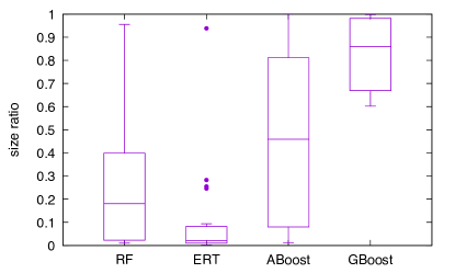
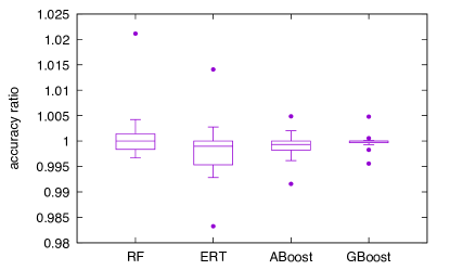
Table 2 shows the results for applying Min_DBN to the classifiers/regressors learned by the four tree ensemble learners from the 21 datasets. The result for each dataset consists of 5 rows, training accuracy (TrA), test accuracy (TeA), the number of distinct branching conditions in the tree ensemble classifier/regressor learned from the training data (NDC), and the ratio of NDC (SR) and accuracy (AR) after applying Min_DBN to the classifier/regressor. Figure 2 shows the distribution of NDC (size) and accuracy ratios over 21 datasets for each tree ensemble learner. You can see that our branching condition sharing reduces the number of distinct branching conditions while keeping test accuracy for all the four tree ensemble learners. Accuracy degradation is within 1% except for the outliers. Our branching condition sharing is most effective for extremely randomized trees (ERTs) and next for random forests (RFs). The size ratio medians for RF and ERT are 18.1% and 2.1%, respectively, and most size ratios are within 10% for ERT. The remarkable outlier dataset for ERT is RNA-Seq PANCAN, whose size ratio is 93.8%, and the size ratios for the other three learners are worse. The number of features in RNA-Seq PANCAN dataset is more than 30 times larger than the number of training instances, and the number of distinct features in each original component decision tree is less than 1/10 of the number of features. As a result, the number of appearing branching conditions for each feature is small, which makes condition sharing difficult. The sharing is also effective for boosting type learners, AdaBoost (ABoost) and gradient boosting (GBoost), whose median size ratios are 45.9% for ABoost and 85.9% for GBoost. Classifiers/Regressors learned by boosting type learners have small NDCs for many datasets, which indicates that their redundancy is small to reduce NDCs significantly.

6.2.2 Effectiveness of using bootstrap training samples per tree

Table 3: Effect of using bootstrap training samples per tree as feature vectors for the tree

dataset	RF	ERT	EI	dataset	RF	ERT	dataset	RF	ERT
iris	0.42004	0.074003	SR(all)①	wave-form	0.18061	0.063826	airfoil	0.11399	0.0019841
	0.35838	0.071344	SR(tree)②		0.16805	0.051071		0.11294	0.0019656
	0.85321	0.96407	②/①		0.93046	0.80016		0.99081	0.99067
	1.0211	1.0141	AR(all)③		1.0042	1.0014		1.0002	0.99960
	1.0141	1.0211	AR(tree)④		1.0033	0.99629		0.99811	0.99455
	0.99310	1.0069	④/③		0.99907	0.99491		0.99787	0.99495
parkin-son	0.39897	0.25483	SR(all)①	robot	0.31750	0.093568	blog-data	0.090640	0.0048244
	0.32510	0.20360	SR(tree)②		0.28016	0.076229		0.088017	0.0045007
	0.81485	0.79896	②/①		0.88238	0.81469		0.97106	0.93291
	1.0000	0.98324	AR(all)③		1.0000	1.0008		1.0014	0.99963
	1.0115	0.97765	AR(tree)④		1.0004	1.0002		1.0024	0.99899
	1.0115	0.99432	④/③		1.0004	0.99943		1.0010	0.99936
breast cancer	0.41953	0.28276	SR(all)①	musk	0.51039	0.24586	Ade-laide	0.017591	0.011090
	0.34647	0.22995	SR(tree)②		0.48205	0.21982		0.016816	0.0094631
	0.82587	0.81324	②/①		0.94446	0.89407		0.95593	0.85328
	1.0018	0.99817	AR(all)③		0.99907	1.0005		0.99837	0.99622
	1.0000	0.99636	AR(tree)④		0.99969	1.0005		0.99791	0.99397
	0.99818	0.99819	④/③		1.0006	1.0000		0.99954	0.99774
blood	0.45025	0.010046	SR(all)①	epi-leptic seizure	0.31092	0.081560	Perth	0.016603	0.010542
	0.39988	0.0098943	SR(tree)②		0.29422	0.066807		0.015871	0.0089568
	0.88812	0.98487	②/①		0.94627	0.81911		0.95589	0.84961
	1.0000	0.99470	AR(all)③		0.99812	0.99532		0.99815	0.99549
	0.99646	0.99823	AR(tree)④		0.99262	0.99381		0.99757	0.99270
	0.99644	1.0035	④/③		0.99448	0.99848		0.99943	0.99720
RNA-Seq PANCAN	0.95551	0.93817	SR(all)①	magic	0.084643	0.028258	Sydney	0.022288	0.014918
	0.94033	0.92062	SR(tree)②		0.076688	0.022711		0.021545	0.013568
	0.98412	0.98130	②/①		0.90602	0.80372		0.96668	0.90950
	1.0000	1.0000	AR(all)③		0.99928	0.99898		0.99868	0.99663
	1.0000	1.0000	AR(tree)④		1.0000	0.99814		0.99832	0.99491
	1.0000	1.0000	④/③		1.0007	0.99916		0.99964	0.99827
wine-quality red	0.21869	0.021399	SR(all)①	hep-mass	0.010160	0.0019280	Tas-mania	0.016625	0.010852
	0.20994	0.019813	SR(tree)②		0.0098652	0.0015365		0.015828	0.0092964
	0.96000	0.92592	②/①		0.97095	0.79695		0.95209	0.85666
	1.0027	0.99370	AR(all)③		0.99996	0.99984		0.99765	0.99410
	1.0090	0.98832	AR(tree)④		0.99991	0.99961		0.99692	0.99030
	1.0063	0.99459	④/③		0.99996	0.99977		0.99927	0.99618
wine-quality white	0.19249	0.010184	SR(all)①	Real estate	0.12487	0.029002	Year Predict MSD	0.010382	0.0044004
	0.18503	0.0094007	SR(tree)②		0.11683	0.025709		0.010117	0.0035825
	0.96123	0.92307	②/①		0.93565	0.88645		0.97448	0.81413
	0.99669	1.0000	AR(all)③		1.0029	1.0028		0.99734	0.99282
	1.0018	1.0003	AR(tree)④		1.0094	1.0043		0.99547	0.98828
	1.0051	1.0003	④/③		1.0065	1.0015		0.99813	0.99542

Figure 3: The box plots of ratios of SR(tree) to SR(all) and AR(tree) to AR(all) for classifiers/regressors learned from the 21 datasets by RF and ERT learners. In the figures, the values outside 1.5 times the interquartile range from the first and third quartile boundaries are plotted as outliers.

Next, we check the effect of using bootstrap training samples per tree as feature vectors for the tree instead of using all the training data as feature vectors for all the trees. The bootstrap training samples per tree can be referred through scikit-learn by building from a little modified source.

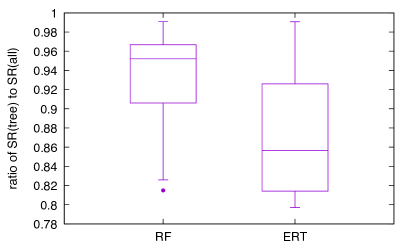
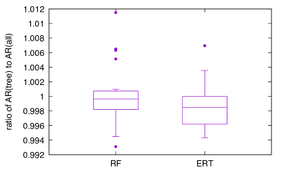
The result is shown in Table 3. In the table, SR(all) and AR(all) are the same as SR and AR in Table 2, and SR(tree) and AR(tree) are SR and AR for the case using each tree’s bootstrap training samples as the feature vectors given to the tree. The ratio of SR(tree) to SR(all) and the ratio of AR(tree) to AR(all) are also shown in the third and sixth rows, respectively, in the rows for each dataset. Figure 3 shows the distributions of those ratios over ensemble classifiers/regressors learned from the 21 datasets by RF and ERT learners. The medians of such relative size ratios for RFs and ERTs are 95.2% and 85.7%, respectively, while also keeping the relative accuracy degradation within 1%.

6.2.3 Effectiveness of further sharing

Figure 4: (accuracy ratio, size ratio)-relation line graphs for two extended Min_DBN and the clustering-based method using k-means (JINGUJI et al., 2018).

Figure 5: Pareto optimal predictors with accuracy ratio more than $0.95$ among the 18 predictors (the clustering-based method using k-means (JINGUJI et al., 2018) with $k=2,4,8,16,32,64,128$, modified Min_DBN with path-changeable-rate $\sigma=0.1,0.2,0.3,0.4,0.5$, another modified Min_DBN using Min_IntSet_wExc that allows $c=0.1,0.2,0.3,0.4,0.5\times$#(intervals for each feature), and original Min_DBN($\sigma=0$ or $c=0$)).

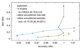
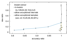
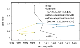
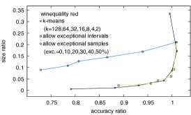
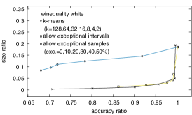
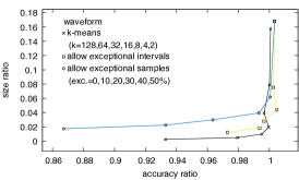
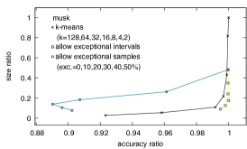
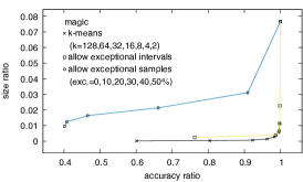
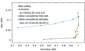
We conduct experiments to check the effectiveness of two extended versions of our branching condition sharing method. One is an extension in which the decision paths of given feature vectors are allowed to change within a given path-changeable rate $\sigma$ at each branching node, that is, an extension allowing exceptional samples. The other is an extension in which $c$ branching condition thresholds are allowed to be out of the path-invariant range for samples passing through the node, that is, an extension allowing exceptional intervals. For the 14 datasets that contain at most 20,000 instances, we run two extended versions of Min_DBN with parameters $100\sigma,100c/p=0,10,20,30,40,50$, where $p$ is the number of intervals for each feature, which depends on a dataset and a feature. We also execute the existing clustering-based method (JINGUJI et al., 2018) in which the centers of $k$-means clustering over the thresholds of branching conditions using the same feature are selected as the thresholds of shared branching conditions. In the experiment, parameter $k$ of the $k$-means clustering-based method is set to $2,4,8,16,32,64$, and $128$.

Figure 4 shows the result of the experiments. Note that the size reduces as exceptions increase for our two methods, and as $k$ decreases for $k$-means clustering-based method. Comparing our two methods, the method allowing exceptional intervals performs better than the method allowing exceptional samples excluding two datasets (blood and epileptic seizure). In most datasets, accuracy degradation by allowing more sample exceptions is larger than that by allowing more interval exceptions though the latter version of Min_DBN needs more memory and computational time than the former version. As for the comparison to $k$-means clustering-based method, the method allowing exceptional interval method performs better for some datasets (parkinson, RNA-Seq PANCAN, robot, musk) but worse for some other datasets (blood, epileptic seizure, airfoil), and similar for the rest 7 datasets. Figure 5 shows pareto optimal predictors among all the predictors with accuracy ratio more than 0.95 for each dataset, that is, predictors that have no predictors better than them in both accuracy and size ratio. The method allowing interval exceptions finds more high accuracy-ratio pareto optimal predictors than the $k$-means clustering-based method.

7 Conclusions

We formalized novel simplification problems of a tree ensemble classifier or regressor, proposed algorithms for the problems, and demonstrated their effectiveness for four major tree ensembles using 21 datasets in the UCI machine learning repository. Our algorithm Min_DBN can make a given tree ensemble share its branching conditions optimally under the constraint that the decision path for any given feature vector does not change, which ensures accuracy preservation. Simple clustering of branching condition thresholds is not easy to find the minimum number of cluster centers that surely keeps accuracy, though it more successfully shares branching conditions with high accuracy for some datasets. Loosening the constraint promotes our method more sharing of branching conditions and achieves a smaller size ratio of the number of distinct branching conditions without accuracy degradation for some datasets.

References

- Andrzejak et al. (2001) RG Andrzejak, K Lehnertz, C Rieke, F Mormann, P David, and Elger CE. Indications of nonlinear deterministic and finite dimensional structures in time series of brain electrical activity: Dependence on recording region and brain state. Phys. Rev. E, 64(061907), 2001.
- Bohanec and Bratko (1994) M. Bohanec and I. Bratko. Trading accuracy for simplicity in decision trees. Machine Learning, 15:223–250, 1994.
- Breiman (2001) Leo Breiman. Random forests. Machine Learning, 45(1):5–32, 2001.
- Breiman et al. (1984) Leo Breiman, Jerome Friedman, Charles J. Stone, and R.A. Olshen. Classification and Regression Trees. Chapman and Hall/CRC, 1984.
- Buza (2012) Krisztian Buza. Feedback prediction for blogs. In Myra Spiliopoulou, Lars Schmidt-Thieme, and Ruth Janning, editors, Data Analysis, Machine Learning and Knowledge Discovery - Proceedings of the 36th Annual Conference of the Gesellschaft für Klassifikation e. V., Hildesheim, Germany, August 2012, Studies in Classification, Data Analysis, and Knowledge Organization, pages 145–152. Springer, 2012. doi: 10.1007/978-3-319-01595-8“˙16. URL https://doi.org/10.1007/978-3-319-01595-8_16.
- Cancer Genome Atlas Research Network et al. (2013) Cancer Genome Atlas Research Network, J N Weinstein, E A Collisson, G B Mills, K R Shaw, B A Ozenberger, K Ellrott, I Shmulevich, C Sander, and J M Stuart. The cancer genome atlas pan-cancer analysis project. Nature genetics, 45(10):1113–1120, 2013.
- Cestnik and Bratko (1991) Bojan Cestnik and Ivan Bratko. On estimating probabilities in tree pruning. In Yves Kodratoff, editor, Machine Learning — EWSL-91, pages 138–150, 1991.
- Chen and Guestrin (2016) Tianqi Chen and Carlos Guestrin. Xgboost: A scalable tree boosting system. In Proceedings of the 22nd ACM SIGKDD International Conference on Knowledge Discovery and Data Mining, page 785–794, 2016.
- Cortez et al. (2009) P. Cortez, A. Cerdeira, F. Almeida, T. Matos, and J. Reis. Modeling wine preferences by data mining from physicochemical properties. Decision Support Systems, 47(4):547–553, 2009.
- Dua and Karra Taniskidou (2017) Dheeru Dua and Efi Karra Taniskidou. UCI machine learning repository, 2017. URL http://archive.ics.uci.edu/ml.
- Esposito et al. (1997) Floriana Esposito, Donato Malerba, and Giovanni Semeraro. A comparative analysis of methods for pruning decision trees. IEEE Trans. Pattern Anal. Mach. Intell., 19:476–491, 1997.
- Freund and Schapire (1997) Yoav Freund and Robert E Schapire. A decision-theoretic generalization of on-line learning and an application to boosting. Journal of Computer and System Sciences, 55(1):119–139, 1997. ISSN 0022-0000. doi: https://doi.org/10.1006/jcss.1997.1504. URL https://www.sciencedirect.com/science/article/pii/S002200009791504X.
- Friedman (2000) Jerome H. Friedman. Greedy function approximation: A gradient boosting machine. Annals of Statistics, 29:1189–1232, 2000.
- Geurts et al. (2006) Pierre Geurts, Damien Ernst, and Louis Wehenkel. Extremely randomized trees. Machine Learning, 63(1):3–42, 2006.
- Gupta et al. (2017) Chirag Gupta, Arun Sai Suggala, Ankit Goyal, Harsha Vardhan Simhadri, Bhargavi Paranjape, Ashish Kumar, Saurabh Goyal, Raghavendra Udupa, Manik Varma, and Prateek Jain. ProtoNN: Compressed and accurate kNN for resource-scarce devices. In Proceedings of the 34th International Conference on Machine Learning, volume 70 of Proceedings of Machine Learning Research, pages 1331–1340. PMLR, 06–11 Aug 2017.
- Hara and Hayashi (2018) Satoshi Hara and Kohei Hayashi. Making tree ensembles interpretable: A bayesian model selection approach. In Proceedings of the Twenty-First International Conference on Artificial Intelligence and Statistics, volume 84 of Proceedings of Machine Learning Research, pages 77–85, 2018.
- Ikeda et al. (2020) Taiga Ikeda, Kento Sakurada, Atsuyoshi Nakamura, Masato Motomura, and Shinya Takamaeda-Yamazaki. Hardware/algorithm co-optimization for fully-parallelized compact decision tree ensembles on fpgas. In Applied Reconfigurable Computing. Architectures, Tools, and Applications: 16th International Symposium, ARC 2020, Toledo, Spain, April 1–3, 2020, Proceedings, page 345–357, 2020.
- (18) Xiangkui Jiang, Chang-an Wu, and Huaping Guo. Forest pruning based on branch importance. Computational Intelligence and Neuroscience, 2017. doi: https://doi.org/10.1155/2017/3162571.
- JINGUJI et al. (2018) Akira JINGUJI, Shimpei SATO, and Hiroki NAKAHARA. An fpga realization of a random forest with k-means clustering using a high-level synthesis design. IEICE Transactions on Information and Systems, E101.D(2):354–362, 2018.
- Kulkarni and Sinha (2012) V. Y. Kulkarni and P. K. Sinha. Pruning of random forest classifiers: A survey and future directions. In 2012 International Conference on Data Science Engineering (ICDSE), pages 64–68, 2012.
- Kumar et al. (2017) Ashish Kumar, Saurabh Goyal, and Manik Varma. Resource-efficient machine learning in 2 KB RAM for the internet of things. In Proceedings of the 34th International Conference on Machine Learning, volume 70 of Proceedings of Machine Learning Research, pages 1935–1944. PMLR, 06–11 Aug 2017.
- Little et al. (2007) Max A Little, Patrick E McSharry, Stephen J Roberts, Declan AE Costello, and Irene M Moroz. Exploiting nonlinear recurrence and fractal scaling properties for voice disorder detection. BioMedical Engineering OnLine, 6(23), 2007.
- Maekawa et al. (2020) Mitsuki Maekawa, Atsuyoshi Nakamura, and Mineichi Kudo. Data-dependent conversion to a compact integer-weighted representation of a weighted voting classifier. In Proceedings of The 12th Asian Conference on Machine Learning, ACML 2020, 18-20 November 2020, Bangkok, Thailand, volume 129 of Proceedings of Machine Learning Research, pages 241–256, 2020.
- Mingers (1989) John Mingers. An empirical comparison of pruning methods for decision tree induction. Machine Learning, 4:227–243, 1989.
- Murshed et al. (2021) M. G. Sarwar Murshed, Christopher Murphy, Daqing Hou, Nazar Khan, Ganesh Ananthanarayanan, and Faraz Hussain. Machine learning at the network edge: A survey. ACM Comput. Surv., 54(8), 2021.
- Nakamura and Sakurada (2019) Atsuyoshi Nakamura and Kento Sakurada. An algorithm for reducing the number of distinct branching conditions in a decision forest. In Machine Learning and Knowledge Discovery in Databases - European Conference, ECML PKDD 2019, Würzburg, Germany, September 16-20, 2019, Proceedings, Part I, volume 11906 of Lecture Notes in Computer Science, pages 578–589, 2019.
- Nan et al. (2016) Feng Nan, Joseph Wang, and Venkatesh Saligrama. Pruning random forests for prediction on a budget. In Advances in Neural Information Processing Systems, volume 29, 2016. URL https://proceedings.neurips.cc/paper/2016/file/3948ead63a9f2944218de038d8934305-Paper.pdf.
- Niblett and Bratko (1987) T. Niblett and I Bratko. Learning decision rules in noisy domains. In Proceedings of Expert Systems ’86, The 6Th Annual Technical Conference on Research and Development in Expert Systems III, page 25–34. Cambridge University Press, 1987.
- Pedregosa et al. (2011) F. Pedregosa, G. Varoquaux, A. Gramfort, V. Michel, B. Thirion, O. Grisel, M. Blondel, P. Prettenhofer, R. Weiss, V. Dubourg, J. Vanderplas, A. Passos, D. Cournapeau, M. Brucher, M. Perrot, and E. Duchesnay. Scikit-learn: Machine learning in Python. Journal of Machine Learning Research, 12:2825–2830, 2011.
- Quinlan (1987) J.R. Quinlan. Simplifying decision trees. International Journal of Man-Machine Studies, 27(3):221–234, 1987. ISSN 0020-7373.
- Vidal and Schiffer (2020) Thibaut Vidal and Maximilian Schiffer. Born-again tree ensembles. In Proceedings of the 37th International Conference on Machine Learning, ICML 2020, 13-18 July 2020, Virtual Event, volume 119 of Proceedings of Machine Learning Research, pages 9743–9753. PMLR, 2020.
- Windeatt and Ardeshir (2001) Terry Windeatt and Gholamreza Ardeshir. An empirical comparison of pruning methods for ensemble classifiers. In Proceedings of the 4th International Conference on Advances in Intelligent Data Analysis, IDA ’01, page 208–217, 2001.
- Yeh and Hsu (2018) I-Cheng Yeh and Tzu-Kuang Hsu. Building real estate valuation models with comparative approach through case-based reasoning. Appl. Soft Comput., 65(C):260–271, apr 2018. ISSN 1568-4946. doi: 10.1016/j.asoc.2018.01.029. URL https://doi.org/10.1016/j.asoc.2018.01.029.
- Yeh et al. (2009) I-Cheng Yeh, King-Jang Yang, and Tao-Ming Ting. Knowledge discovery on rfm model using bernoulli sequence. Expert Systems with Applications, 36(3):5866–5871, 2009.
- Zhang et al. (2006) Yi Zhang, Samuel Burer, and W. Nick Street. Ensemble pruning via semi-definite programming. J. Mach. Learn. Res., 7:1315–1338, dec 2006.