Evidence of high latitude emission in the prompt phase of GRBs:
How far from the central engine are the GRBs produced?

Abstract

The physical mechanism of gamma-ray bursts (GRBs) remains elusive. One of the difficulties in nailing down their physical mechanism comes from the fact that there has been no clear observational evidence on how far from the central engine the prompt gamma-rays of GRBs are emitted while the competing physical mechanisms predict different characteristic distances. Here we present a simple study addressing this question by making use of the “high-latitude emission” (HLE). We show that our detailed numerical modeling exhibits a clear signature of HLE in the decaying phase of “broad pulses” of GRBs. We show that the HLE can emerge as a prominent spectral break in $F_{\nu}$ spectra and dominate the peak of $\nu F_{\nu}$ spectra even while the “line-of-sight emission” (LoSE) is still ongoing, hence providing a new view of HLE emergence. We remark that this “HLE break” could be hidden in some broad pulses, depending on the proximity between the peak energies of the LoSE and the HLE. Also, we present three examples of Fermi-GBM GRBs with broad pulses that exhibit the HLE signature. We show that their gamma-ray emitting region should be located at $\sim 10^{16}$ cm from the central engine, which disfavors the photosphere models and small-radii internal shock models but favors magnetic dissipation models with a large emission radius.

1 Introduction

The gamma-ray bursts (GRBs) are believed to invoke highly relativistic jets with bulk Lorentz factors of a few hundreds (Kumar & Zhang, 2015). For such a highly relativistic jet, the relativistic beaming and boosting of radiation plays an important role and gives rise to interesting results especially when combined with a spherical geometry of the emitting surface. The photons emitted from a jet location with high latitude, called the “high-latitude emission” (HLE), take longer to reach a distant observer and are boosted with a smaller Doppler factor than the photons traveling along the line of sight, called the “line-of-sight emission” (LoSE). These two aspects of HLE are known as the “curvature effect” of a relativistic spherical jet. It is known that the HLE satisfies a simple relation (Kumar & Panaitescu, 2000; Dermer, 2004; Uhm & Zhang, 2015), $\hat{\alpha}=2+\hat{\beta}$, between the temporal index $\hat{\alpha}$ and the spectral index $\hat{\beta}$ in the convention of $F_{\nu_{\rm obs}}\propto t_{\rm obs}^{-\hat{\alpha}}\,\nu_{\rm obs}^{-\hat{\beta}}$ if the emitter remains a constant Lorentz factor. Here, $F_{\nu_{\rm obs}}$ is the observed spectral energy flux, $t_{\rm obs}$ the observer time, and $\nu_{\rm obs}$ the observed frequency. This relation was generalized later for relativistic jets that undergo bulk acceleration ($\hat{\alpha}>2+\hat{\beta}$) or bulk deceleration ($\hat{\alpha}<2+\hat{\beta}$) (Uhm & Zhang, 2015).

The curvature effect of HLE is commonly invoked to account for the steep decay of X-ray and $\gamma$-ray flares seen in the afterglow phase of GRBs (Liang et al., 2006; Uhm & Zhang, 2016a; Jia et al., 2016; Ajello et al., 2019) as well as during the steep-decay phase of X-ray emission following the prompt emission (Zhang et al., 2006, 2009). As for the prompt phase of GRBs, several studies (Ryde & Petrosian, 2002; Kocevski et al., 2003; Genet & Granot, 2009; Shenoy et al., 2013) have investigated the role that the curvature effect has on temporal and spectral properties of individual pulses, but an unambiguous identification of HLE could not be achieved.

The prompt phase of GRBs contains an important observational feature called the “broad pulses”. Observationally, the broad pulses exhibit two distinct patterns of peak evolution; i.e., the peak-energy ($E_{p}$) of $\nu F_{\nu}$ spectra shows a “hard-to-soft” or a “flux-tracking” pattern across the pulses (Ford et al., 1995; Norris et al., 1996; Golenetskii et al., 1983; Lu et al., 2012). In addition, the light curves of broad pulses in different energy bands exhibit a sequential pattern in their peak time, known as the “spectral lags” (Norris et al., 1996, 2000; Kocevski & Liang, 2003); softer emission lags behind harder emission (“positive” type) in most cases, whereas harder emission can lag behind softer emission (“negative” type) in some cases. The curvature effect of HLE was traditionally suggested as a plausible explanation for the positive type of spectral lags (Shen et al., 2005), but a detailed study (Uhm & Zhang, 2016b) showed that the HLE cannot give rise to any spectral lags if the spectral shape is softer than $F_{\nu_{\rm obs}}\propto\nu_{\rm obs}^{2}$. The HLE may produce some spectral lags for a spectral shape harder than this $\nu_{\rm obs}^{2}$, but the resulting spectral lags are essentially invisible due to the significant flux-level difference between the light curves (Uhm & Zhang, 2016b).

The complex and intriguing characteristics of broad pulses carry crucial clues to unveil the nature of GRBs. For instance, a series of numerical studies (Uhm & Zhang, 2016b; Uhm et al., 2018) showed that all those features of broad pulses can be successfully reproduced within a single physical picture that invokes a bulk acceleration of the emitting region and that keeps the LoSE ongoing across the production of broad pulses. Also, Li & Zhang (2021) found evidence of jet acceleration in an effort of searching for the curvature effect.

Here, we present a simple study that identifies a clear signature of HLE in the decaying phase of broad pulses and provide a new understanding on the HLE emergence. We also present three examples of Fermi-GBM (Meegan et al., 2009) GRBs that exhibit the HLE signature in their broad pulses.

2 A simple physical model

Following the previous works (Uhm & Zhang, 2016b; Uhm et al., 2018), we adopt a simple physical picture where a thin, relativistic spherical shell expands in space radially. The radiating electrons are distributed uniformly in the shell and emit synchrotron photons (Rybicki & Lightman, 1979) isotropically in the co-moving frame. Then we take fully into account the curvature effect to compute the HLE (Uhm & Zhang, 2015). We assume a “Band” function shape (Band et al., 1993) for the emission spectrum in the co-moving frame since the observed gamma-ray spectra are traditionally fit to this function and since it is a good representation of synchrotron radiation (Uhm & Zhang, 2014; Zhang et al., 2016). The strength of magnetic field $B(r)$ in the emitting region globally decreases as the radius $r$ from the central engine increases, which is expected for a spherical jet traveling in space. We note that this was the essential physical element to explain the low-energy photon index of the Band spectra for the majority of GRBs (Uhm & Zhang, 2014; Geng et al., 2018). Moreover, the emitting region itself undergoes rapid bulk acceleration (Uhm & Zhang, 2016a, b) during which the prompt gamma-rays are produced; i.e., the bulk Lorentz factor $\Gamma(r)$ of the region has an increasing profile in radius $r$. Also, the characteristic Lorentz factor $\gamma_{\rm ch}(r)$ of electrons in the co-moving frame is allowed to evolve with radius $r$.

We present three numerical models of broad pulses: Model [u], [v], and [w]. The three models have different $\gamma_{\rm ch}(r)$ profile as described in Appendix A. Other than $\gamma_{\rm ch}$ profile, we keep all other model parameters the same for the three models, for simplicity. We assume a Band-function shape with typical low- and high-energy photon spectral index $\alpha_{\rm B}=-0.8$ and $\beta_{\rm B}=-2.3$, respectively, for the emission spectrum in the co-moving frame. The number of radiating electrons is assumed to increase at a constant injection rate $R_{\rm inj}=10^{47}$ $\mbox{s}^{-1}$. The bulk Lorentz factor of the jet takes a power-law profile in radius $r$, $\Gamma(r)=\Gamma_{0}(r/r_{0})^{s}$, with $\Gamma_{0}=250$, $r_{0}=10^{15}$ cm, and $s=0.35$, as used in Uhm & Zhang (2016b). We turn on the emission of spherical jet at radius $r_{\rm on}=10^{14}$ cm and turn off its emission at radius $r_{\rm off}=3\times 10^{16}$ cm. For the given profile of $\Gamma(r)$, this turning-off happens at about $t_{\rm obs}=4.0$ sec. We stress that the LoSE remains ongoing until this turn-off time. The magnetic field strength $B(r)$ in the co-moving frame also takes a power-law profile, $B(r)=B_{0}(r/r_{0})^{-b}$, with $B_{0}=30$ G and $b=1.5$ (Uhm & Zhang, 2016b). We calculate the luminosity distance to GRB for a flat $\Lambda$CDM universe with parameters $\Omega_{\rm m}=0.31$, $\Omega_{\rm\Lambda}=0.69$, and $H_{0}=68$ km/s/Mpc (Planck Collaboration et al., 2016) and take a typical value of redshift $z=1$.

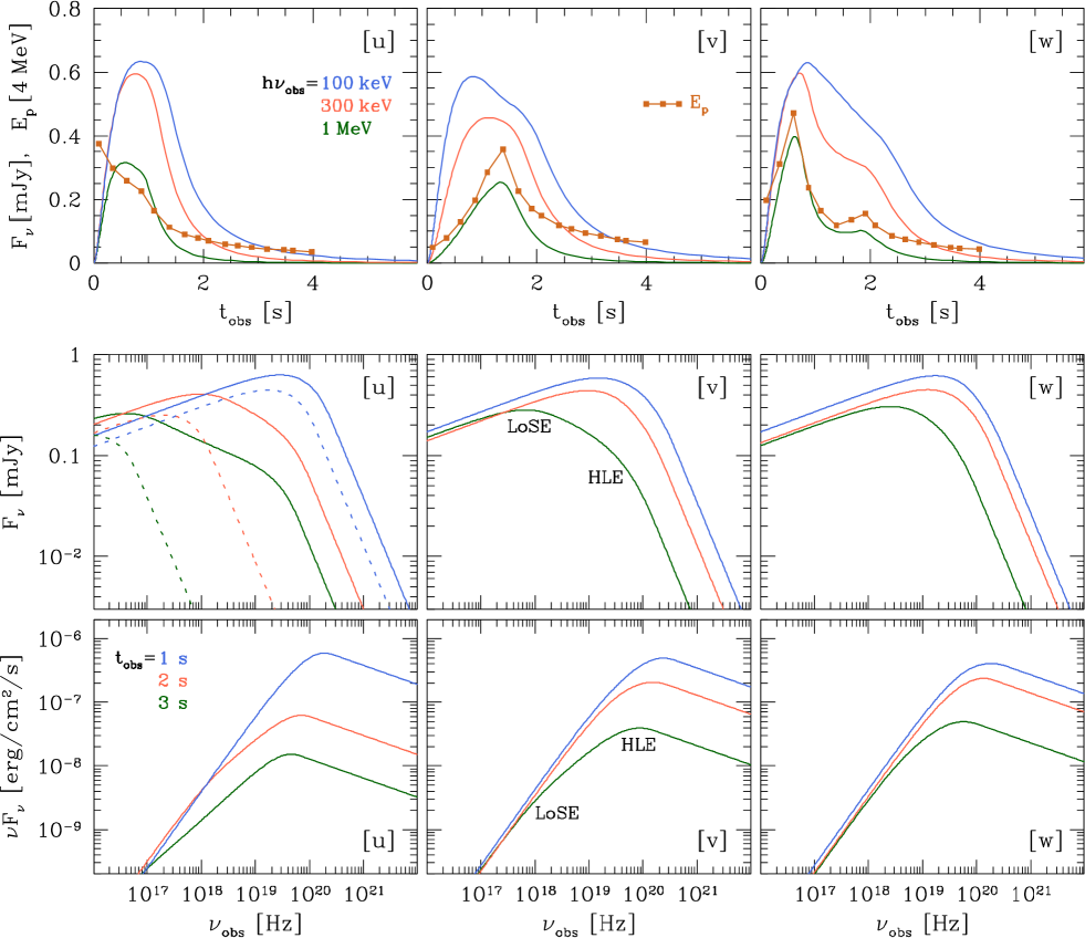
Figure 1: Light curves and time-dependent spectra of our numerical models [u], [v], and [w]. The top panels show the light curves at 100 keV, 300 keV, and 1 MeV, together with temporal evolution of $E_{p}$ curves. The middle panels show time-dependent spectra at 1 sec, 2 sec, and 3 sec, with the curvature effect of HLE (Uhm & Zhang, 2015) fully included (solid lines) or removed (dotted lines) for model [u]. The $\nu F_{\nu}$ spectra in the bottom panels are derived from the corresponding solid lines in the middle panels.

Figure 1 shows a modeling result of the three models [u], [v], and [w]. The top panels show the light curves at 100 keV, 300 keV, and 1 MeV, which exhibit both the positive and negative types of spectral lags. The top panels also show the temporal evolution of $E_{p}$ curves exhibiting both the hard-to-soft and the flux-tracking patterns across the pulses. The middle panels show the time-dependent spectra at 1 sec, 2 sec, and 3 sec (solid lines). In the co-moving frame, we inject a Band-function spectrum with fixed $\alpha_{\rm B}$ and $\beta_{\rm B}$. However, the resulting spectra in the observer frame deviate significantly from this single Band function. Hence, in order to understand this deviation, we repeat the same calculations without considering the curvature effect; the resulting spectra are shown in dotted lines in the middle panel for model [u]. Comparing the solid and dotted lines, one can clearly see that the curvature effect causes the deviation and that the HLE emerges as a prominent additional spectral break in $F_{\nu}$ spectra during the decaying phase of the broad pulses. We again stress that the jet emission is not turned off until about 4 sec in our models and, therefore, the LoSE is still active and dominates the peak of $F_{\nu}$ spectra as it should. The bottom panels show the $\nu F_{\nu}$ spectra directly calculated from the solid lines in the middle panels, in which it is clear that the “HLE break” ($\nu_{\rm\scriptscriptstyle HLE}$) in $F_{\nu}$ spectra now becomes the peak energy ($E_{p}$) in $\nu F_{\nu}$ spectra in the decaying phase of these broad pulses.

If the peak of $\nu F_{\nu}$ spectra is dominated by the HLE, there should exist a simple scaling relation

$$F_{\nu,E_{p}}\propto E_{p}^{\,2},$$ (1)

expected from the HLE theory (Dermer, 2004; Uhm & Zhang, 2015). Here, $F_{\nu,E_{p}}$ is the spectral energy flux $F_{\nu}$ measured at the peak energy $E_{p}$.

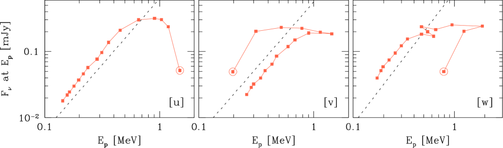
Figure 2: The peak energy $E_{p}$ vs the spectral flux $F_{\nu}$ at $E_{p}$ (i.e., $F_{\nu,E_{p}}$) across the broad pulses of our numerical models [u], [v], and [w]. An open circle in each model marks the first point in the beginning of pulses. The dotted line indicates the relation $F_{\nu,E_{p}}\propto E_{p}^{\,2}$ in Equation (1).

In Figure 2, we plot $F_{\nu,E_{p}}$ against $E_{p}$ across the broad pulses of three numerical models [u], [v], and [w]. An open circle in each model marks the first point in the beginning of the pulse. One can clearly see that the model curves closely follow Equation (1) (indicated by the dotted line) in the decaying phase of broad pulses, ascertaining that the peak of $\nu F_{\nu}$ spectra indeed originates from the HLE. This is the clear signature of HLE, produced in our numerical models of broad pulses.

3 Data Analysis

Fermi-GBM (Meegan et al., 2009) has accumulated invaluable observations for the prompt emission of GRBs. In search of the HLE signature above, we analyzed a sample of Fermi-GBM GRBs with broad pulses. We require a certain minimum on the observed fluence to select bright GRBs and then perform a Bayesian-block analysis and impose several criteria to collect relatively clean broad-pulses. We then perform a time-resolved spectral analysis on each GRB selected. Details on the analysis are presented in an accompanying paper (Tak et al. 2023, submitted).

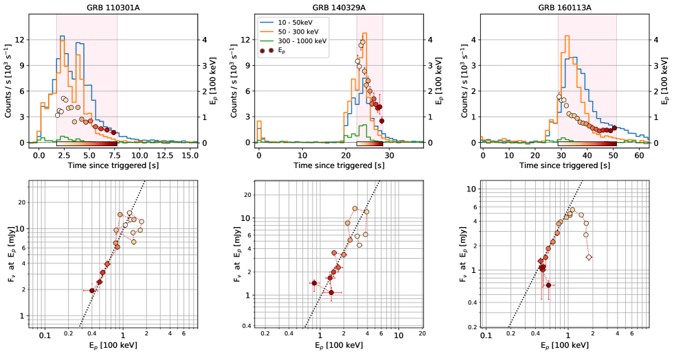
Figure 3: Results of our time-resolved spectral analysis performed on three example broad pulses in GRB 110301A, GRB 140329A, and GRB 160113A. The top panels show the light curves at three different energy bands, together with temporal evolution of $E_{p}$ points. The bottom panels show the $E_{p}$ vs $F_{\nu,E_{p}}$ points obtained from the analysis. The dotted line indicates the relation $F_{\nu,E_{p}}\propto E_{p}^{\,2}$ in Equation (1). The color gradient in the bottom panels is in accordance with the color gradient encoded in $E_{p}$ points in the top panels.

In Figure 3, we present three examples: GRB 110301A, GRB 140329A, and GRB 160113A. The top panels show the light curves at three different energy bands, together with the temporal evolution of $E_{p}$ curves. The bottom panels show $E_{p}$ vs $F_{\nu,E_{p}}$ obtained from the time-resolved spectral analysis. The dotted line indicates the theoretical HLE relation in Equation (1). As one can see, the $F_{\nu,E_{p}}$ - $E_{p}$ points obtained from the time-resolved analysis of the three bursts are in good agreement with Equation (1) in the decaying phase of their broad pulse, implying that the HLE signature is indeed identified. The color gradient used in the bottom panels is in accordance with the color gradient encoded in $E_{p}$ points in the top panels, which helps locate where in the pulse the HLE signature starts to show up.

4 Conclusions and Discussion

In this paper, we showed that the HLE can imprint a clear spectral signature in prompt-emission gamma-ray spectra (i.e., additional spectral break $\nu_{\rm\scriptscriptstyle HLE}$ in $F_{\nu}$ spectra and peak energy in $\nu F_{\nu}$ spectra) in the existence of ongoing LoSE. This result provides a new view regarding the HLE, because it has been believed so far that the HLE can show up and dominate the spectra only after the LoSE is turned off.

We remark, on the other hand, that the HLE spectral break is not required to appear in all broad pulses. It is because the HLE break could be buried under the LoSE component when the peak energy of LoSE (at a given time) is not far below that of HLE (emitted at earlier times but belonging to the same equal-arrival-time surface). Whether this condition is satisfied or not would depend on the physical parameters in the emitting region. Therefore, this new perspective on the HLE emergence provides flexibility to elucidate both detection and non-detection of HLE signatures in observations of broad pulses.

In this paper, we also showed that some Fermi-GBM broad pulses exhibit the HLE scaling relation between $E_{p}$ and $F_{\nu,E_{p}}$ (Equation 1) in their decaying phase.

The HLE signature observed in some broad pulses leads to important implication regarding the emission radius of GRBs. The HLE emitted at radius $r$ is received at an observer time given roughly by $t_{\rm obs}\sim r/(2c\,\Gamma^{2})$ like in the case of LoSE, which yields

$$r\sim 2c\,\Gamma^{2}\,t_{\rm obs}=(1.6\times 10^{16}\,\mbox{cm})\left(\frac{\Gamma}{300}\right)^{2}\,\left(\frac{t_{\rm obs}}{3\,\mbox{s}}\right),$$ (2)

where $c$ is the speed of light. The duration of broad pulses in our examples is tens of seconds, and therefore the gamma-ray emitting region of those GRBs with HLE signature should be located at $\sim 10^{16}$ cm from the central engine for a typical value of $\Gamma=300$.

This inference of the emission radius is robust (i.e., independent of details of our modeling) and sheds light on differentiating the GRB models. The estimated large emission radius $\sim 10^{16}$ cm is consistent with the ICMART model (Zhang & Yan, 2011), which invokes collision-induced magnetic dissipation as the origin of GRB prompt emission. In contrast, the photospheric emission models (Lazzati et al., 2013) and the internal shock models (Rees & Mészáros, 1994) are disfavored since the photospheric radii and the internal shock radii are typically at $\sim 10^{11}-10^{12}$ cm and at $\sim 10^{13}-10^{14}$ cm, respectively (Kumar & Zhang, 2015).

In short, we identified a clear signature of HLE in the prompt phase of GRBs both theoretically and observationally. Also, we presented a unique constraint on the validity of the competing GRB models.

Appendix A Profile of characteristic Lorentz factor $\gamma_{\rm ch}$ of electrons

The characteristic Lorentz factor $\gamma_{\rm ch}(r)$ of electrons evolves in radius $r$ in our models. Considering the energy dissipation and particle acceleration process, which would depend, for instance, on the degree of magnetic energy dissipation, it is plausible to assume that the $\gamma_{\rm ch}$-profile evolves in radius as the emitting shell expands in space. The model [u] has a broken power-law profile

$$\gamma_{\rm ch}(r)=\left\{\begin{array}[]{ll}\gamma_{\rm ch}^{0}(r/r_{0})^{g_{1}}&\mbox{if}\quad r<r_{0},\\ \gamma_{\rm ch}^{0}(r/r_{0})^{-g_{2}}&\mbox{if}\quad r\geq r_{0},\end{array}\right.$$ (A3)

with $\gamma_{\rm ch}^{0}=10^{5}$, $r_{0}=10^{15}$ cm, $g_{1}=1/2$, and $g_{2}=1$. The model [v] also takes the same form of broken power-law but with $\gamma_{\rm ch}^{0}=2\times 10^{5}$, $r_{0}=2\times 10^{15}$ cm, and $g_{1}=g_{2}=1$. The model [w] has a profile made of four power-law segments

$$\gamma_{\rm ch}(r)=\left\{\begin{array}[]{ll}\gamma_{\rm ch}^{0}(r/r_{1})&\mbox{if}\quad r<r_{1},\\ \gamma_{\rm ch}^{0}(r/r_{1})^{-1}&\mbox{if}\quad r_{1}\leq r<r_{2},\\ 2\gamma_{\rm ch}^{0}(r/r_{3})&\mbox{if}\quad r_{2}\leq r<r_{3},\\ 2\gamma_{\rm ch}^{0}(r/r_{3})^{-1}&\mbox{if}\quad r_{3}\leq r,\end{array}\right.$$ (A8)

with $\gamma_{\rm ch}^{0}=10^{5}$, $r_{1}=5\times 10^{14}$ cm, $r_{2}=10^{15}$ cm, and $r_{3}=4\times 10^{15}$ cm. These three $\gamma_{\rm ch}$ profiles are shown in Figure 4.

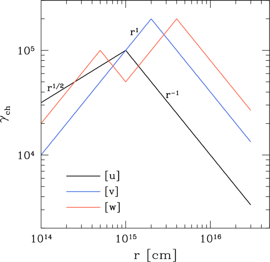
Figure 4: Profile of characteristic Lorentz factor $\gamma_{\rm ch}$ of electrons in our numerical models [u], [v], and [w].

References

- Ajello et al. (2019) Ajello, M., Arimoto, M., Asano, K., et al. 2019, ApJ, 886, L33
- Band et al. (1993) Band, D., Matteson, J., Ford, L., et al. 1993, ApJ, 413, 281
- Dermer (2004) Dermer, C. D. 2004, ApJ, 614, 284
- Ford et al. (1995) Ford, L. A., Band, D. L., Matteson, J. L., et al. 1995, ApJ, 439, 307
- Genet & Granot (2009) Genet, F., & Granot, J. 2009, MNRAS, 399, 1328
- Geng et al. (2018) Geng, J.-J., Huang, Y.-F., Wu, X.-F., Zhang, B., & Zong, H.-S. 2018, ApJS, 234, 3
- Golenetskii et al. (1983) Golenetskii, S. V., Mazets, E. P., Aptekar, R. L., & Ilinskii, V. N. 1983, Nature, 306, 451
- Jia et al. (2016) Jia, L.-W., Uhm, Z. L., & Zhang, B. 2016, ApJS, 225, 17
- Kocevski & Liang (2003) Kocevski, D., & Liang, E. 2003, ApJ, 594, 385
- Kocevski et al. (2003) Kocevski, D., Ryde, F., & Liang, E. 2003, ApJ, 596, 389
- Kumar & Panaitescu (2000) Kumar, P., & Panaitescu, A. 2000, ApJ, 541, L51
- Kumar & Zhang (2015) Kumar, P., & Zhang, B. 2015, Phys. Rep., 561, 1
- Lazzati et al. (2013) Lazzati, D., Morsony, B. J., Margutti, R., & Begelman, M. C. 2013, ApJ, 765, 103
- Li & Zhang (2021) Li, L., & Zhang, B. 2021, ApJS, 253, 43
- Liang et al. (2006) Liang, E. W., Zhang, B., O’Brien, P. T., et al. 2006, ApJ, 646, 351
- Lu et al. (2012) Lu, R.-J., Wei, J.-J., Liang, E.-W., et al. 2012, ApJ, 756, 112
- Meegan et al. (2009) Meegan, C., Lichti, G., Bhat, P. N., et al. 2009, ApJ, 702, 791
- Norris et al. (2000) Norris, J. P., Marani, G. F., & Bonnell, J. T. 2000, ApJ, 534, 248
- Norris et al. (1996) Norris, J. P., Nemiroff, R. J., Bonnell, J. T., et al. 1996, ApJ, 459, 393
- Planck Collaboration et al. (2016) Planck Collaboration, Ade, P. A. R., Aghanim, N., et al. 2016, A&A, 594, A13
- Rees & Mészáros (1994) Rees, M. J., & Mészáros, P. 1994, ApJ, 430, L93
- Rybicki & Lightman (1979) Rybicki, G. B., & Lightman, A. P. 1979, Radiative processes in astrophysics (New York, Wiley-Interscience, 1979. 393 p.)
- Ryde & Petrosian (2002) Ryde, F., & Petrosian, V. 2002, ApJ, 578, 290
- Shen et al. (2005) Shen, R.-F., Song, L.-M., & Li, Z. 2005, MNRAS, 362, 59
- Shenoy et al. (2013) Shenoy, A., Sonbas, E., Dermer, C., et al. 2013, ApJ, 778, 3
- Uhm & Zhang (2014) Uhm, Z. L., & Zhang, B. 2014, Nature Physics, 10, 351
- Uhm & Zhang (2015) —. 2015, ApJ, 808, 33
- Uhm & Zhang (2016a) —. 2016a, ApJ, 824, L16
- Uhm & Zhang (2016b) —. 2016b, ApJ, 825, 97
- Uhm et al. (2018) Uhm, Z. L., Zhang, B., & Racusin, J. 2018, ApJ, 869, 100
- Zhang et al. (2006) Zhang, B., Fan, Y. Z., Dyks, J., et al. 2006, ApJ, 642, 354
- Zhang & Yan (2011) Zhang, B., & Yan, H. 2011, ApJ, 726, 90
- Zhang et al. (2016) Zhang, B.-B., Uhm, Z. L., Connaughton, V., Briggs, M. S., & Zhang, B. 2016, ApJ, 816, 72
- Zhang et al. (2009) Zhang, B.-B., Zhang, B., Liang, E.-W., & Wang, X.-Y. 2009, ApJ, 690, L10