Significantly Improving Zero-Shot X-ray Pathology Classification
via Fine-tuning Pre-trained Image-Text Encoders

Abstract

Deep neural networks have been successfully adopted to diverse domains including pathology classification based on medical images. However, large-scale and high-quality data to train powerful neural networks are rare in the medical domain as the labeling must be done by qualified experts. Researchers recently tackled this problem with some success by taking advantage of models pre-trained on large-scale general domain data. Specifically, researchers took contrastive image-text encoders (e.g., CLIP) and fine-tuned it with chest X-ray images and paired reports to perform zero-shot pathology classification, thus completely removing the need for pathology-annotated images to train a classification model. Existing studies, however, fine-tuned the pre-trained model with the same contrastive learning objective, and failed to exploit the multi-labeled nature of medical image-report pairs. In this paper, we propose a new fine-tuning strategy based on sentence sampling and positive-pair loss relaxation for improving the downstream zero-shot pathology classification performance, which can be applied to any pre-trained contrastive image-text encoders. Our method consistently showed dramatically improved zero-shot pathology classification performance on four different chest X-ray datasets and 3 different pre-trained models (5.77% average AUROC increase). In particular, fine-tuning CLIP with our method showed much comparable or marginally outperformed to board-certified radiologists (0.619 vs 0.625 in F1 score and 0.530 vs 0.544 in MCC) in zero-shot classification of five prominent diseases from the CheXpert dataset.

1 Introduction

The success of deep neural networks (DNNs) for visual and textual data led to them being widely adopted in diverse domains and tasks including the pathology classification based on medical images. Although there were a few success stories in adopting neural networks for medical images such as classification of diabetic retinopathy [13, 19] and skin cancer [12], a wider adoption is hindered by their nature of requiring a large amount of high-quality training samples. This poses a great challenge especially in the medical imaging domain, as qualified experts are required to create labeled samples, not to mention the difficulty of collecting images to begin with as they require special machinery.

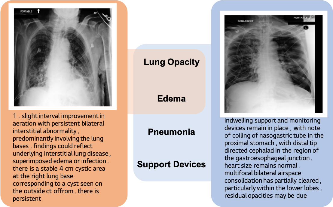
Figure 1: Example of false negatives between medical data. Two image-text pairs share two classes of disease; lung opacity and edema. Existing image-text contrastive learning frameworks deal other pair as perfectly negative one.

Recent studies tackled this problem with some success by taking advantage of the powerful pre-trained models trained on large-scale general domain data. Some demonstrated that fine-tuning a pre-trained image encoder in a supervised manner can yield impressive performance [23, 17, 3]. This approach, however, still requires some amount of expert-annotated images. Another approach, demonstrated by CheXzero [30], relies on image-text multi-modal encoder such as CLIP [27] to perform pathology classification without requiring any labeled images. CLIP is self-supervisingly trained via contrastive learning on approximately 400M image-text pairs, therefore capable of extracting generalizable representations from images and text, even demonstrated impressive zero-shot classification that outperformed supervised training in lots of datasets [27].

CheXzero harnessed CLIP’s generalization capability by fine-tuning it with over than 200,000 pairs of chest X-ray images and reports to perform zero-shot pathology classification, successfully matching the performance of board-certified radiologists. This demonstrated that, by combining the power of a heavily pre-trained model with a moderate amount of domain-specific image-text pairs, it is possible to perform pathology classification even without having to construct an expert-annotated training set.

Meanwhile, medical image-report pairs have multi-labeled nature that we should consider about. For example, let us imagine two chest X-ray studies where one has Lung Opacity, Edema, Pneumonia, Support Devices, and the other has the first two. Then, their reports must at least share the semantics of Lung Opacity and Edema (See Fig. 1), which we term partial positive. CheXzero, however, uses the vanilla contrastive learning, which regards partial positive pairs as completely negative pairs, which leads the model to learn suboptimal image-text representations. MedCLIP [31], another zero-shot pathology classification study, partially addresses this issue but requires expert labels to do so.

In this work, we propose a new fine-tuning strategy for zero-shot pathology classification by taking into account the multi-label nature of medical image-text pairs. Our method does not require any explicit labels, and can be applied to any pre-trained contrastive image-text encoders to improve the downstream zero-shot performance. Our method consists of sentence sampling and loss relaxation, which are based on two core observations: 1) Every sentence in a report contains important clinical information; 2) There are many false negative pairs, but practically no perfectly positive pairs. Our fine-tuning strategy produced consistent improvement in zero-shot pathology classification when applied to three pre-trained models on four different chest X-ray datasets, even sometimes marginally outperforming board-certified radiologists in one dataset. We further empirically proved the efficacy of our method on image-text alignment, where our method also demonstrated consistent performance improvement.

The contribution of this work is summarized below:

• In this paper, we propose a new fine-tuning strategy for zero-shot pathology classification from unannotated X-ray images. Our method does not need explicit labels, and can be applied to any pre-trained contrastive image-text encoders.

• Using four different chest X-ray datasets and three different pre-trained models, we show that the proposed method consistently improves the zero-shot pathology classification performance, with an average AUROC increase of 5.77%.

• Especially for the CheXpert dataset, fine-tuning CLIP with our method sometimes outperformed board-certified radiologists marginally in detecting five prominent diseases with 0.619 vs 0.625 in F1 scores and 0.530 vs 0.544 in MCC.

• Our fine-tuning strategy also showed consistent performance improvement for image-text alignment. Ablation studies were simultaneously conducted to verify the effectiveness of the proposed fine-tuning method.

2 Related works

Vision-text representation learning in medical domain   Following the success of large-scale image-text pre-training in the general domain, such as CLIP, medical image-text representation learning has been explored. ConVIRT [34] first proposed contrastive learning for the medical domain. ConVIRT [34] trained on paired medical images and reports via a bidirectional contrastive objective. GloRIA [14] focused on using global and local alignment. CheXzero [30] is the state-of-the-art method for achieving an expert-level zero-shot multi-pathology classification. However, these models fail to properly address the false negative cases, i.e., image-report pair with the same label from different patients. MedCLIP [31] designs a semantic similarity matrix between image and text as a soft target to eliminate false negatives. However, they need annotated data to define their objective function. Our method, on the other hand, achieves improved zero-shot classification performance compared to SOTA without any additional labels.

Text augmentation   Token-level augmentation, such as random insertion or deletion, is commonly used in the general domain regardless of the length of the input text [4]. However, this has a high risk of information loss since medical reports are composed of short information-intensive sentences. Sentence-level method [4], like back translation or text generation, also can be used but not guaranteed to preserve certain medical semantics. In the medical domain, Abdollahi et al. [1] tried to replace extracted medical concepts with corresponding scientific names in the Unified Medical Language System (UMLS). This method is limited in that it requires both a powerful extraction tool and external medical knowledge. Alternatively, we propose a simple yet powerful augmentation method, i.e. sentence-level random selection that preserves each sentence’s content as it is, without additional knowledge.

Loss relaxation for contrastive learning    Some studies try to improve the performance of contrastive learning by adjusting the loss function. Wu et al. [32] and Xie et al. [33] explore negative sampling methods. To avoid making training too hard or easy, Wu et al. [32] selects negative samples in a ring around each positive by distances in the feature space. Xie et al. [33] chooses a semi-negative sample from each instance’s top 10% nearest neighbors. On the other hand, Cho et al. [7] propose masked contrastive learning (MCL), with the regularization loss function that decreases the level of repulsion between positive view pairs (i.e., samples with the same class). MCL shows better class-conditional clustering in feature space. This method is similar to our loss relaxation method in that it controls the degree of repel for positive pairs but has the disadvantage of requiring label information. Our loss relaxation ensures that image-report pairs with the same semantic from different patients are not pushed too far apart by restraining the push of samples with cosine similarity greater than $t$, without label information.

3 Methods

In this section, we propose two fine-tuning strategies for improving zero-shot multi-pathology recognition from unannotated X-ray images. Please refer to Appendix for pseudo codes of the methods. First, we briefly explain the concept of “zero-shot” to demonstrate our methods. We present (1) sentence-level text augmentation for medical report, and (2) loss regularization to overcome data insufficient issue and false-negative problem (i.e., images and reports from different patients have same semantics, but incorrectly considered as negative pairs) in medical domain.

3.1 Zero-shot X-ray pathology classification

Zero-shot evaluation refers to the process of training or tuning a model using a large-scale dataset, and subsequently assessing its performance on a range of different data sets without requiring any further fine-tuning (i.e., cross-dataset zero-shot) [27, 28]. In this paper, we focus on the zero-shot X-ray pathology classification task defined by CheXzero [30]. First, we jointly train an image encoder $E_{img}$ and a text encoder $E_{txt}$ to predict the correct image-text pairs through InfoNCE loss (Fig. 4(a)). We do not use manual labels for X-ray image for training. To perform the zero-shot classification, we use the similarity between the image embedding for the target unseen X-ray image $\textbf{I}_{trg}$ and the text embedding for the pathology prompts $\textbf{T}_{c}$ of pathology c, which belong to C of the target dataset classes. First, we construct positive and negative prompts, $\textbf{T}_{+,c}$ and $\textbf{T}_{-,c}$, for each pathology $c$. Then we calculate the softmax probability of each pathology through the cosine similarity between the target image embedding and the embedding of the positive / negative prompt (Fig. 4(b)).

$$s_{+,c}=E_{img}(\textbf{I}_{trg})\cdot E_{txt}(\textbf{T}_{+,c}),$$ (1)

$$s_{-,c}=E_{img}(\textbf{I}_{trg})\cdot E_{txt}(\textbf{T}_{-,c}),$$

$$prob_{c}=\text{softmax}(s_{+,c},\;s_{-,c}),$$

where $c$ indicate target pathology, $s_{+,c}$ and $s_{-,c}$ are cosine similarity of positive and negative prompt, respectively.

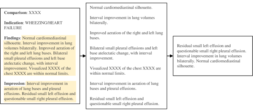
Figure 2: Example of text augmentation. Given original free-form report (Left), we extract only ”Findings” and ”Impression” section, and split them into sentences (Middle). $n$ sentences are randomly selected to make new positive text pairs (Right).

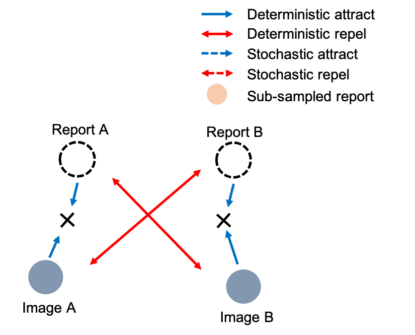
(a) Use of whole report

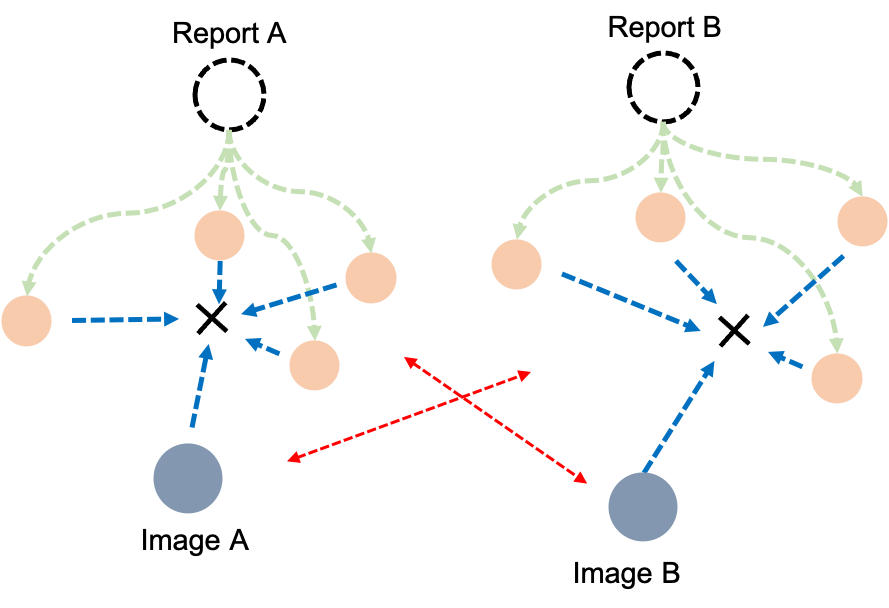
(b) Use of sub-sampled reports

Figure 3: Effect of random text augmentation. (a) When using the whole report, negative pairs deterministically repel each other. (b) However, when using random text augmentation, an image can stochastically attract various positive sub-sampled reports in each epoch.

3.2 Random text augmentation

In contrast to the general domain, the medical domain has a scarcity of large-scale and high-quality datasets because they require annotations from medical experts, which are laborious to obtain. Text augmentation is the most widely used solution to solve data shortage. However, due to the specific nature of medical reports, it is challenging to use the augmentation techniques that are typically used in general domains. Medical reports consist of meaningful content for diagnosis, and most of the sentences are short and formal (Fig. 2 (left)). Each sentence generally includes a description of different diseases or anatomical findings. Therefore, text augmentation at the token level, such as random deletion or switch, can be harmful to maintaining the correct clinical meaning of reports.

We propose a simple but effective text augmentation without any supervision to tackle this issue. We randomly subsample $n$ sentences from the report for every sample and feed them into the contrastive learning framework. Suppose that the number of sentences in the report is $m$, then the image can be matched ${}_{m}C_{n}$ positive samples by stochastic subsampling. Through this, the model can learn the rich semantics of each sentence rather than train with only one positive pair.

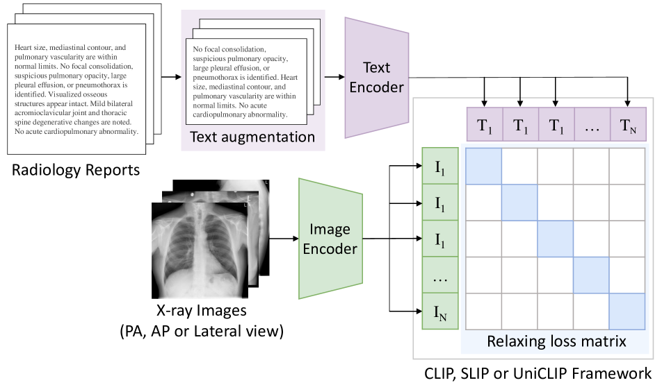
(a) Contrastive fine-tuning

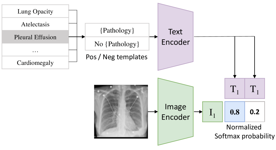
(b) Zero-shot pathology classification

Figure 4: (a) Overall of our fine-tuning strategies, text augmentation and relaxation loss, on contrastive learning frameworks with a medical multi-modal dataset. Our proposed methods could be easily applied to various image-text contrastive learniinig framework, such as CLIP, SLIP, and UniCLIP. (b) Zero-shot pathology classification. Text encoder works as a multi-label classifier by embedding the names or descriptions of the target dataset’s pathologies at test time.

3.3 Loss for relaxed image-text agreement

CLIP [27] jointly trains an image encoder and a text encoder to predict the correct pairings of image-text pairs. Given a batch of $N$ image-text pairs, CLIP maximizes the similarity between $N$ positive pairs while minimizing the similarity between $N^{2}-N$ negative pairs by the InfoNCE loss [25], as follows.

$$\mathcal{L}=-\frac{1}{2N}(\sum_{i=1}^{N}log\frac{exp(\textbf{sim}(u_{i},v_{i})/\tau)}{\sum_{j=1}^{N}exp(\textbf{sim}(u_{i},v_{j})/\tau)}+$$ (2)

$$\sum_{i=1}^{N}log\frac{exp(\textbf{sim}(v_{i},u_{i})/\tau)}{\sum_{j=1}^{N}exp(\textbf{sim}(v_{i},u_{j})/\tau)})$$

where $u,v$ are the normalized vectors from the image and text encoders and $(u_{i},v_{i})$ is a positive pair. sim is a function to calculate the similarity between two vectors, and $\tau$ denotes the learnable temperature.

However, the CLIP objective function does not consider false negative cases, which have similar semantics but are treated as negative pairs. Unfortunately, false negative pairs (Fig. 1) are more likely to occur due to the fine-grained label scope of the medical domain compared to the general domain. Thus, forcing an increase in similarity only for positive pairs, despite the existence of false-negative samples, can lead to confusion for the model. We argue that reducing the attraction between positive pairs can alleviate this problem. We propose the modified sim function that makes the model focus on perfectly negative pairs (images or reports from different patients with different semantics) instead of false negative pairs by clipping the upper bound of the similarity function.

$$\textbf{sim}(u_{i},v_{j})=\left\{\begin{array}[]{ll}\frac{1}{1+\exp(-\alpha(u_{i}\cdot v_{j}-t))}&,\begin{matrix}\text{ if }i=j\text{ and }\\ u_{i}\cdot v_{j}\geq t\end{matrix}\\ \\ u_{i}\cdot v_{j}/2t&,\begin{matrix}\text{ else if }i=j\text{ and }\\ t>u_{i}\cdot v_{j}\geq 0\end{matrix}\\ \\ u_{i}\cdot v_{j}&,\text{ otherwise}\end{array}\right.$$ (3)

, where $u_{i}\cdot v_{j}$ denotes cosine similarity between two vectors, $\alpha$ a slope coefficient of the Sigmoid function. A threshold of $t$ ($0<t<1$) is used to determine the level of attractiveness between positive pairs. With our modified similarity function, positive pairs with a similarity score $\textbf{sim}(u_{i}\cdot v_{i})\geq t$ quickly reach a maximum similarity value (i.e., loss of that pairs become minimum). Note that we separately defined the second and third terms of Eq. 3 for the continuity of the sim function when $u_{i}\cdot v_{i}=0$ and $u_{i}\cdot v_{i}=t$.

4 Experiments

In this section, we explore the contribution of our proposed fine-tuning strategy in the medical domain to zero-shot performance in three CLIP-based frameworks. We show that we can achieve performance close to or marginally exceed the expert level using our method without label information. We verify that we can get close to the expert level or marginally exceed using our method without label information. We also verify that the learned representations through the image-text alignment task.

		$\#$ of Images	$\#$ of Reports	$\#$ of classes
Fine-tuning	MIMIC-CXR [16]	377,110	227,835	-
	CheXpertvalid [15]	234	-	14
Evaluation	CheXperttest [15]	668	-	14
	Open-i [2]	2,550	2,550	14
	PadChest [5]	15,091	15,091	61
	VinDr-CXR [24]	3,000	-	20

Table 1: The statistics of datasets.

4.1 Datasets

MIMIC-CXR [16]

The MIMIC-CXR is a large-scale public database that includes 377,110 chest radiographs corresponding to 227,835 studies in free-text format. We use this dataset for fine-tuning. Since meaningful observations are mainly written in the ”Findings” or ”Impression” sections, we extract those two sections for each study. If the section is not extracted by the rule-base method, we use the last paragraph of those samples. All radiographs are used for fine-tuning regardless of views (AP, PA, and lateral).

CheXpert [15]

The CheXpert is a public dataset that includes 224,316 chest radiographs of 65,240 patients from Stanford Hospital, annotated with 14 classes. The validation and test sets have 234 and 668 images, respectively. We use CheXpert’s validation set for model selection and the testset for evaluation. We select the model by mean AUC of the validation set over the five CheXpert competition tasks: Atelectasis, Cardiomegaly, Consolidation, Edema, Pleural Effsion . For evaluation, we deal with 13 labels of CheXpert, except for ”no finding” since predicting all labels as zero has the same no finding in a multi-label setting.

PadChest [5]

The PadChest is a public dataset provided by the Medical Imaging Databank of the Valencia Region. This dataset consists of more than 160,000 chest radiograph images of 67,000 patients from San Juan Hospital (Spain) from 2009 to 2017. PadChest is annotated with 174 different findings and 19 differential diagnoses. We used only 15,091 examples ($n=15,091$) as a test set, which board-certified radiologists manually annotated. We used 61 radiographic findings where $n>100$ in the testset. We use PadChest test set to evaluate zero-shot classification performance and image-text alignment.

Open-i chest X-ray dataset

Open-i collection [8] is a service for abstract and image search by the National Library of Medicine (NLM). The Open-i chest radiograph dataset includes 7,470 images and 3,955 reports provided by Indiana University Hospital. We select the ”Finding” and ”Impression” sections which contain essential information associated with the X-ray images. We first select the image-text pair with frontal view images and filtered samples with a report length of 10 characters or more. We use preprocessed dataset with 2,550 image-text pairs as our test set to evaluate image-text similairty and zero-shot classification. For reference, the data is labelled by CheXpert-labeler provided by the authors [15].

VinDr-CXR

[24] This chest X-ray dataset includes 18,000 images, 150,000 for the train set and 3,000 for the test set, collected from two major hospitals in Vietnam. Total 17 board-certificated radiologists annotated them with 28 labels consisting of 22 local abnormalities and 6 global suspected diseases. Each scan in the test set was labeled by the consensus of 5 radiologists. We evaluated zero-shot classification for 20 labels with more than 10 samples within the test set.

Dataset statistics and their usage in this paper are summarized in Tab. 1.

4.2 Baselines

In this paper, we fine-tune three CLIP-based frameworks with proposed methods to show the effect of our strategy.

• CLIP [27]: CLIP (Contrastive Language-Image Pre-training) is a multi-modal contrastive learning framework pre-trained on 400M image-text pairs. CLIP uses InfoNCE loss to maximize mutual information of latent vectors from image and text encoders.

• SLIP [22]: SLIP is a multi-task learning framework that enhances the representation quality by combining image self-supervised learning with CLIP pre-training.

• UniCLIP [20]: UniCLIP is a unified framework for visual–language pre-training that improves data efficiency by integrating inter- and intra-domain pairs’ contrastive loss into a single universal space.

Note that the CLIP framework with ViT-B/16 without our proposed method is the same as the CheXzero setting, except for the image encoder architecture.

	CheXpert		Open-i		PadChest	VinDr-CXR
	avg. 5 AUC	avg. total AUC	avg. 5 AUC	avg. total AUC	avg. total AUC	avg. total AUC
CLIP	0.870 ± 0.006	0.771 ± 0.001	0.785 ± 0.030	0.691 ± 0.010	0.685 ± 0.026	0.801 ± 0.020
CLIP w/ ours	0.885 ± 0.007	0.789 ± 0.017	0.808 ± 0.008	0.708 ± 0.013	0.725 ± 0.014	0.842 ± 0.007
SLIP	0.831 ± 0.008	0.722 ± 0.008	0.760 ± 0.008	0.666 ± 0.004	0.684 ± 0.004	0.799 ± 0.018
SLIP w/ ours	0.884 ± 0.009	0.779 ± 0.020	0.810 ± 0.016	0.719 ± 0.018	0.741 ± 0.005	0.831 ± 0.009
UniCLIP	0.851 ± 0.008	0.741 ± 0.037	0.744 ± 0.032	0.643 ± 0.027	0.684 ± 0.009	0.759 ± 0.019
UniCLIP w/ ours	0.888 ± 0.006	0.802 ± 0.018	0.788 ± 0.016	0.694 ± 0.006	0.717 ± 0.011	0.843 ± 0.016
CheXzero	0.844 ± 0.008	0.733 ± 0.008	0.771 ± 0.006	0.684 ± 0.006	0.702 ± 0.011	0.771 ± 0.024
MedCLIP∗	0.880	0.829	0.794	0.728	0.728	0.829

• $\ast$: use label information defined in CheXpert for training

Table 2: Zero-shot classification performance on three different CLIP-based frameworks on the four different datasets (mean ± std). Best performance is in bold. For the CheXpert and Open-i datasets, the average AUC of five CheXpert competition pathologies and a total of 13 pathologies are reported. For the PadChest and VinDr-CXR dataset, an average of 61 pathologies ($n>100$) and 20 pathologies ($n>10$) is reported.

4.3 Implemetation Details

We used the $\text{BERT}_{\text{base}}$ model [10] as text encoder and ViT-B/16 [11] as image encoder for three CLIP-based frameworks as described above (i.e., CLIP, SLIP, UniCLIP). For CLIP and UniCLIP, we initialize the model using the publicly available pre-trained weight provided by OpenAI. In the case of SLIP, we use the model checkpoint that was pre-trained with the YFCC-15M dataset [29] for initialization.

For the random text augmentation, three sentences ($n=3$) are sampled from each report. The relaxation loss threshold $t$ is 0.5, and the slope coefficient $\alpha$ is fixed at 10. The type of image augmentation applied varies depending on the CLIP framework, and the details are summarized in the appendix. We set the image resolution to $224\times 224$. We implement the entire model in Pytorch [26] and train the entire network for 50 epochs with a batch size of 1024 using 8 GPUs of the A100 server (NVIDIA Crop.). We use the Adam optimizer [18] with an initial learning rate $1\times 10^{-4}$ and decay the learning rate using a cosine schedule with a warm-up for 100 iterations[21]. We repeat all experiments three times with different random seeds and report the mean and standard deviation. Although our CheXpert testset includes lateral view images, the CheXzero model was trained and tested only on PA and AP view images. Thus, we retrained CheXzero with our training set for a fair comparison. MedCLIP uses additional image/text supervision for 14 main entity types for training. Since the training data are not publicly open, we compare the evaluation performance using the pre-trained model provided by the authors.

4.4 Evaluation tasks

4.4.1 Zero-Shot Classification

We perform a zero-shot multi-label image classification on four datasets; CheXpert, PadChest, Open-i, and VinDr-CXR. We use prompts of ’{label}’ and ’no {label}’ following Tiu et al. [30] (e.g., ”Atelectasis” and ”No atelectasis”). For CheXpert and Open-i, we use all 13 pathologies. In the case of PadChest, we use 61 of 193 labels with more than 100 patients with that label. Finally, VinDR-CXR is evaluated with 20 of 28 labels being included more than 20 patients. The macro AUC (Area under the ROC Curve) for multi-label is used as an evaluation matrix.

4.4.2 Image-Text Alignment

In a medical report, each sentence generally contains different label information. Therefore, measuring the image-text alignment not only report-level but also sentence-level can indicate how learned embedding contains semantics for each label. We calculate the cosine similarity between image embedding and report embedding for each X-ray-Report pair for report-level evaluation. We also calculate the average similarity between the image and sentence embedding for all sentences in the corresponding report to measure sentence-level alignment.

5 Results and Discussion

	mean AUC	Mean F1	Mean MCC
Radiologists (mean) [30]	-	0.619	0.530
CLIP	0.870	0.578	0.423
CLIP w/ ours	0.885	0.603	0.443
CLIP${}_{\text{ensemble}}$	0.887	0.613	0.519
CLIP${}_{\text{ensemble}}$ w/ ours	0.893	0.614	0.525
SLIP	0.831	0.578	0.423
SLIP w/ ours	0.884	0.608	0.424
SLIP${}_{\text{ensemble}}$	0.845	0.564	0.456
SLIP${}_{\text{ensemble}}$ w/ ours	0.893	0.625	0.537
UniCLIP	0.851	0.561	0.458
UniCLIP w/ ours	0.888	0.610	0.522
UniCLIP${}_{\text{ensemble}}$	0.881	0.614	0.524
UniCLIP${}_{\text{ensemble}}$ w/ ours	0.900	0.623	0.544
CheXzero	0.844	0.559	0.417
CheXzero${}_{\text{ensemble}}$	0.857	0.576	0.480
MedCLIP∗	0.880	0.625	0.537

• $\ast$: use label information defined in CheXpert for training

Table 3: Comparison with the performance of three board-certified radiologists on CheXpert test dataset (mean ± std). We also report the comparison between the ensemble over the best model checkpoints from 3 runs with a different random seed. We report the average results across the five CheXpert competition pathologies. The mean AUC of radiologists is not available, as radiologist predictions are only binary. The colored cell means that the model outperformed the prediction performance of the expert radiologist. The best performance is in bold, and the second best is in underline for each framework.

Zero-Shot Classification We empirically validate that our fine-tuning strategies consistently improve the zero-shot classification performance on 4 independent datasets collected from four different countries: CheXpert, Open-i, PadChest and VinDR-CXR. CheXpert and Open-i are evaluated on the same CheXpert 13 labels. PadChest and VinDR-CXR are evaluated on 61 labels and 20 labels, respectively. A list of all labels used for evaluation is in the Appendix.

To analyze the effect of our proposed method, we experimented with a three different frameworks. In Tab. 2, we demonstrate the effectiveness and generalizability of our method by showing consistent results in different label spaces and data distribution. We show significant improvements compared to baseline (i.e. with our fine-tuning strategy) performance in all three frameworks and four datasets. Average 5.77% increase in AUROC is observed in zero-shot classification. For details, CLIP baseline improved by 3.4% increase, SLIP by 6.86%, and UniCLIP by 7.05%.

These results mean that our method successfully embeds the multi-pathology feature, reflecting the nature of the medical data well. In addition, we also show that ensembling selected models based on their performance in validation sets at each random seed bring significant improvements in all cases (Tab. 3). We also show that the model can perform comparable pathology classification performance with board-certified radiologists using our method in Tab. 3. Furthermore, in the case of SLIP and UniCLIP, they outperform the expert-level by adopting our strategy with ensembles.

We compare our results with existing state-of-the-art models for medical image-text presentation learning in Tab. 2 and Tab. 3. For single model without an ensemble, we outperform CheXzero on all datasets. In addition, our method also shows enhanced performance in all other metrics except the total AUC of Open-i. Surprisingly, although MedCLIP trained using CheXpert’s 14 label information, our model outperforms or performs similarly without any label information.

	Open-i		PadChest
	sentence-level	report-level	sentence-level	report-level
CheXzero	0.319 ± 0.015	0.387 ± 0.015	0.232 ± 0.079	0.258 ± 0.081
CLIP	0.275 ± 0.053	0.407 ± 0.007	0.102 ± 0.099	0.135 ± 0.111
CLIP w/ ours	0.658 ± 0.005	0.693 ± 0.005	0.572 ± 0.021	0.579 ± 0.015
SLIP	0.163 ± 0.021	0.287 ± 0.031	0.007 ± 0.022	0.018 ± 0.014
SLIP w/ ours	0.434 ± 0.034	0.489 ± 0.035	0.512 ± 0.008	0.500 ± 0.009
UniCLIP	0.209 ± 0.013	0.318 ± 0.016	0.096 ± 0.010	0.118 ± 0.011
UniCLIP w/ ours	0.451 ± 0.038	0.543 ± 0.024	0.396 ± 0.060	0.418 ± 0.068
MedCLIP∗	0.044	0.047	0.040	0.047

Table 4: Image-text similarity for Open-i and PadChest datasets (mean ± std). We report both sentence-level similarity and report-level similarity for each dataset.

	Text aug	Relax loss	Atelectasis	Cardiomegaly	Consolidation	Edema	Pleural Effusion	avg. 5 AUC	avg. total AUC
CLIP			0.828 ± 0.016	0.845 ± 0.012	0.895 ± 0.007	0.861 ± 0.016	0.878 ± 0.020	0.861 ± 0.002	0.787 ± 0.044
		$\checkmark$	0.858 ± 0.009	0.815 ± 0.013	0.889 ± 0.023	0.875 ± 0.022	0.890 ± 0.006	0.865 ± 0.002	0.794 ± 0.045
	$\checkmark$		0.864 ± 0.004	0.867 ± 0.008	0.904 ± 0.015	0.903 ± 0.003	0.877 ± 0.021	0.883 ± 0.005	0.820 ± 0.001
	$\checkmark$	$\checkmark$	0.859 ± 0.006	0.840 ± 0.016	0.913 ± 0.010	0.881 ± 0.009	0.869 ± 0.012	0.872 ± 0.005	0.824 ± 0.003
SLIP			0.760 ± 0.046	0.788 ± 0.008	0.877 ± 0.028	0.847 ± 0.021	0.902 ± 0.010	0.835 ± 0.010	0.791 ± 0.015
		$\checkmark$	0.826 ± 0.010	0.828 ± 0.010	0.899 ± 0.006	0.873 ± 0.013	0.899 ± 0.010	0.865 ± 0.005	0.828 ± 0.003
	$\checkmark$		0.830 ± 0.022	0.837 ± 0.021	0.864 ± 0.042	0.899 ± 0.008	0.876 ± 0.013	0.861 ± 0.004	0.800 ± 0.015
	$\checkmark$	$\checkmark$	0.845 ± 0.014	0.855 ± 0.018	0.904 ± 0.014	0.905 ± 0.016	0.868 ± 0.009	0.875 ± 0.006	0.819 ± 0.028
UniCLIP			0.774 ± 0.060	0.833 ± 0.012	0.869 ± 0.016	0.856 ± 0.033	0.882 ± 0.020	0.843 ± 0.010	0.750 ± 0.016
		$\checkmark$	0.840 ± 0.009	0.818 ± 0.021	0.870 ± 0.012	0.869 ± 0.014	0.897 ± 0.021	0.859 ± 0.008	0.808 ± 0.023
	$\checkmark$		0.860 ± 0.012	0.862 ± 0.010	0.900 ± 0.019	0.879 ± 0.005	0.887 ± 0.012	0.877 ± 0.009	0.790 ± 0.020
	$\checkmark$	$\checkmark$	0.870 ± 0.007	0.844 ± 0.007	0.911 ± 0.002	0.886 ± 0.014	0.882 ± 0.017	0.878 ± 0.001	0.825 ± 0.028

Table 5: Ablation study of different components of our proposed method on the CheXpert validation set (mean ± std). We report the zero-shot classification performance on three different CLIP-based frameworks. Best performance is in bold and second best is in underline for each framework. For the CheXpert dataset, the AUC for each of the five competition pathologies, the average value of these five pathologies, and the total of 13 pathologies of this dataset are reported.

Image-Text Alignment We analyze how our method affects the semantic presentation quality of the model through the alignment of image-text at the sentence level and the report level. Based on the observation that each sentence in the medical report usually contains different clinical findings, we hypothesize that measuring the sentence level could evaluate whether the model utilizes multi-label information in a fine-grain scale. As seen in Tab. 4, both sentence-level and report-level similarity increases significantly with our method. At the same time, our method reduces the similarity gap between the sentiment-level and report-level measurement of each dataset.

Our text augmentation prevents the representation overfitting only a part of the report by randomly selecting sentences from paired reports corresponding to the query image. It allows our model to focus on important pathology information in each sentence and aggregate it to learn report-level embeddings with rich semantics. Additionally, due to the nature of the medical domain, this learning method can reduce the domain gap between different datasets. Medical reports are often written concisely with essential information, and the form of sentences is limited. Therefore, even if the overall data distribution is different, the model might show robust domain generalization performance with recognition ability at the sentence level. The results in Tab. 4 support this argument. Padchest has a more significant gap in training data than open-i since PadChest reports are written in Spanish. Without our method, all frameworks have significant differences between open-i and padchest performance. However, our method shows a significant performance improvement while reducing these gaps.

Ablation Study We analyze and evaluate the effectiveness of the components of our method by comparing the zero-shot pathology classification performance on the CheXpert test set. In Tab. 5, we verify the benefit of each method. Even when text augmentation and loss relaxing are used independently, they show improved average AUC over baseline. While loss relaxation indirectly allows false-negative cases, Text augmentation directly increases the diversity of training data, encouraging the model to learn robust embedding. Thus, as shown in rows 2 and 3 of Table 2, the performance improvement gap was more significant when only text augmentation was applied. We can observe that the contributions for improvement differ according to pathology. Pleural effusion was mainly improved by the relax loss, while the others were improved by the text augmentation. In most cases, the performance reaches to the optimum when applied both methods, sometimes get to the sub-optimum though. We additionally show the effects of hyper-parameters of our strategy by evaluating the zero-shot classification with various hyper-parameters in Fig. 5. Following this observation, we use the text augment hyper-parameter as $n=3$, and the relaxing loss hyper-parameter as $t=0.5$.

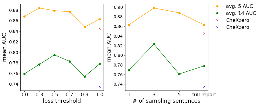
Figure 5: Effect of the relaxing threshold (left) and the number of sampling sentences of text augmentation (right). Both evaluate the performance of zero-shot classification on the CheXpert validation set.

	$n=1$	$n=2$	$n=3$	$n=4$	$n=5$
avg. $\#$ of report	8433.86	538.40	106.20	25.24	1.03

Table 6: Average number of reports which contains same label combinations for CheXpert label.

Analysis of false-negative keys Text sampling can generate false-negative pairs, since sentences extracted through random sampling can have the same labels. Tab. 6 shows that, on average, $8,433$ reports share one label, $538$ two labels, etc. From Tab. 6 and Fig. 5, we can conclude that sampling three sentences per report makes a great compromise between the number of false negatives and the effectiveness of contrastive learning. Note that there still exists partial overlap between sampled sentences, but this is addressed by our loss relaxation.

6 Conclusion

In this paper, we propose a simple yet effective fine-tuning strategy for medical image-text multi-modal learning. Our method consists of two ways, random sentence sampling, and loss relaxation, to reflect the multi-label nature of the medical image-text data. Our fine-tuning strategy improves zero-shot pathology classification performance in all three CLIP-based frameworks. In addition, our proposed method significantly outperformed board-certified radiologists without additional label information for two frameworks. Further, we validate the effect of our method through image-text alignment tasks on two radiography datasets. Although our model shows enough comparable (or sometimes exceeding) performance compared to the expert level in pathology classification performance, it is difficult to determine whether judgments are made based on where the pathology occurred. For future work, we plan to explore the medical multi-modal representation learning method that can consider these localized features.

Supplementary

1 Implementation details for the frameworks

1.1 Similarity matrices

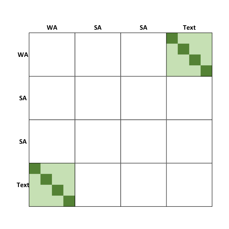
(a) CLIP

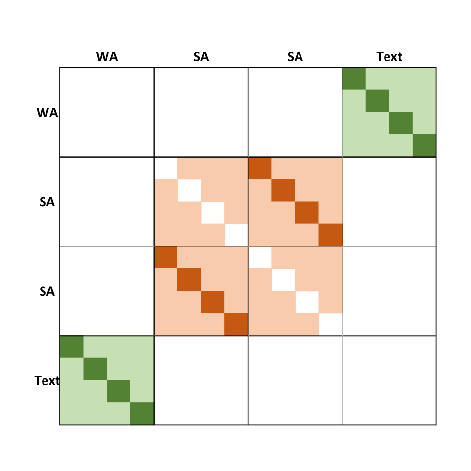
(b) SLIP

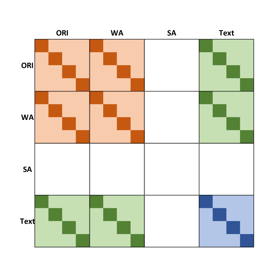
(c) UniCLIP

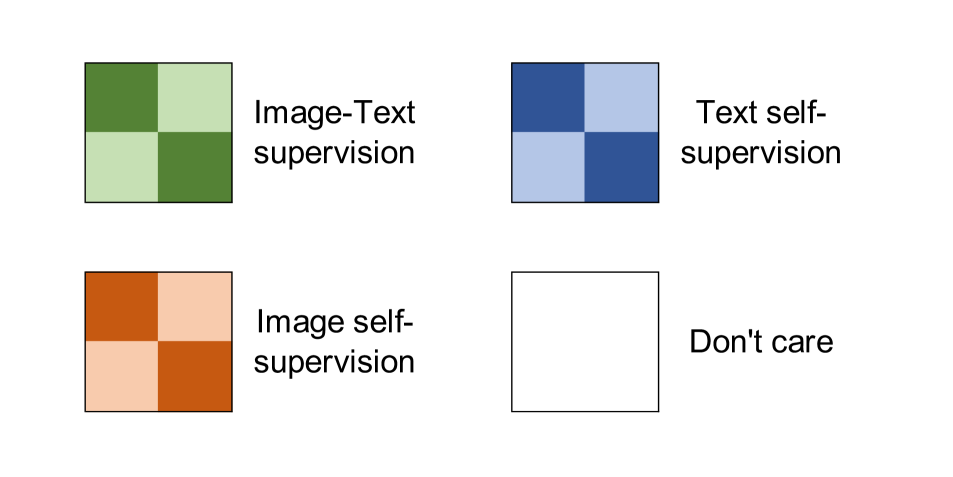
Figure 6: Similarity matrices of the frameworks used in this paper. Darker colors represent positive pairs and lighter colors negative them. ORI: Original image, WA: Weakly Augmented image, SA: Strongly Augmented image

Fig. 6 shows the similarity matrices of the frameworks used in this paper. For weakly augmented image (WA), we randomly sampled rotation (-20, 20), resized crop with scale (0.8, 1.0) and ratio (0.9, 1.1), horizontal flip (true or false) and color jitter with the brightness (0.5, 2) and contrast (0.5, 2). The hue is not adjusted due to the monochronic nature of the X-ray images. For strongly augmented image (SA), the ranges of rotation and the resized crop were expanded as follows: rotation (-30, 30), resized crop with scale (0.7, 1.0) and ratio (0.8, 1.2).

1.2 Design of loss relaxation

Section 3.3 of the main paper explains our loss relaxation for positive pairs. The repelling force between negative pairs can also be relaxed as well as positive pairs. There was no difference in performance when relaxation with a threshold ($-t$) was applied to the negative pair compared to not using this relaxation. This is because the labels of the medical domain are more fine-grained than the general domain, so the similarity of the negative pairs is biased in the positive direction. Thus, we focus on relaxing the loss for only positive pairs.

1.3 Contrastive loss functions

We describe the contrastive loss function of each framework used in this paper.

1.3.1 CLIP loss

$$l_{i}^{u\rightarrow v}=-\log{{\exp{(\textbf{sim}(u_{i},v_{i})/\tau)}}\over{\sum_{j=1}^{N}}\exp{(\textbf{sim}(u_{i},v_{j})/\tau)}}$$ (4)

, where $u,v$ are normalized vectors of the image and text encoders, respectively. $(u_{i},v_{i})$ is a positive pair, sim is a function to calculate the similarity between the vectors and $\tau$ means the learnable temperature. $N$ is the mini-batch size of image-text pairs. $l_{i}^{u\rightarrow v}$ means the InfoNCE loss from the image $i$ to the texts, and $l_{i}^{v\rightarrow u}$ means vice versa. Then, the final loss in CLIP is as follows.

$$\mathcal{L}_{\text{CLIP}}=\frac{1}{2N}\sum_{i=1}^{N}\left({l_{i}^{u\rightarrow v}+l_{i}^{v\rightarrow u}}\right)$$ (5)

1.3.2 SLIP loss

First, there are two sets of images strongly augmented (SA) from the original set ($2N$ SA images). Then, the SA image $i$ and $i+N$ get paired as positive construct self-supervised loss (SSL) as in the following.

$$l_{i}^{\text{SSL}}=\left\{\begin{array}[]{ll}-\log{\frac{\exp({\textbf{sim}(u_{i},u_{i+N}})/\tau)}{\sum_{j\neq i}^{2N}\exp(\textbf{sim}(u_{i},u_{j})/\tau)}}&\text{, if~{}~{}}i<N\\ \\ -\log{\frac{\exp({\textbf{sim}(u_{i},u_{N-i}})/\tau)}{\sum_{j\neq i}^{2N}\exp(\textbf{sim}(u_{i},u_{j})/\tau)}}&\text{, otherwise}\end{array}\right.$$ (6)

The total SSL loss for SA pairs is

$$\mathcal{L}_{\text{SSL}}=\frac{1}{2N}\sum_{i=1}^{2N}l_{i}^{\text{SSL}}$$ (7)

We define the SSL loss following the Chen et al. [6]. The final loss of the SLIP framework is the sum of the CLIP loss (Eq. 5) and the SSL loss (Eq. 7) as follows.

$$\mathcal{L}_{\text{SLIP}}=\mathcal{L}_{\text{CLIP}}+\mathcal{L}_{\text{SSL}}$$ (8)

1.3.3 UniCLIP loss

UniCLIP integrates the contrastive loss of both inter-domain and intra-domain pairs into a single universal space. Let us suppose three sets of ORI, WA, and Text. For the mini-batch size $N$, the feature vectors are yielded in $z_{i},~{}z_{i+N},~{}z_{i+2N}$, respectively. Then, the UniCLIP loss for each sample is computed as follows.

The final loss of UniCLIP is as follows.

$$\mathcal{L}_{\text{UniCLIP}}=\frac{1}{3N}\sum_{i=1}^{3N}l_{i}^{\text{UniCLIP}}$$ (10)

Please note that the augmentation feature embedding of UniCLIP was ignored in this paper because strong augmentation such as large crop ratio and RGB adjustment is useless in X-ray images.

1.4 Pseudo codes

Pseudo codes for fine-tuning with CLIP, SLIP, and UniCLIP are presented below.

  Algorithm 1 Fine-tuning with CLIP

  $N$: mini-batch size,
$f_{I}$: image encoder, $f_{T}$: text encoder,
$u$: normalized encoded image vector,
$v$: normalized encoded text vector,
$I$: input image, $T$: input text,
WA: weak augmentation, TA: random text augmentation

1:for $iteration=1,2,\ldots$ do

2:    for $i=1,\ldots,N$ do

3:        $u_{i}=f_{I}(\text{WA}(I_{i}))$

4:        if use text augmentation is True then

5:           $v_{i}=f_{T}(\text{TA}(T_{i}))$

6:        else

7:           $v_{i}=f_{T}(T_{i})$

8:        end if

9:    end for

10:    for $i=1,\ldots,N$ do

11:        for $j=1,\ldots,N$ do

12:           if use relaxing loss is True and $i==j$ then

13:               sim$(u_{i},v_{j})$ = Compute Eq. (3) in the main paper

14:           else

15:               sim$(u_{i},v_{j})=u_{i}\cdot v_{j}$

16:           end if

17:        end for

18:        Compute $l_{i}^{u\rightarrow v}$ and $l_{i}^{v\rightarrow u}$

19:    end for

20:    Optimize Eq. 5

21:end for

 

  Algorithm 2 Fine-tuning with SLIP

  $N$: mini-batch size,
$f_{I}$: image encoder, $f_{T}$: text encoder,
$u$: normalized encoded image vector,
$v$: normalized encoded text vector,
$I$: input image, $T$: input text,
WA: weak augmentation, SA: strong augmentation,
TA: random text augmentation

1:for $iteration=1,2,\ldots$ do

2:    for $i=1,\ldots,N$ do

3:        $u_{i}=f_{I}(\text{WA}(I_{i}))$

4:        $u_{i+N}=f_{I}(\text{SA}(I_{i}))$

5:        $u_{i+2N}=f_{I}(\text{SA}(I_{i}))$ #another SA

6:        if use text augmentation is True then

7:           $v_{i}=f_{T}(\text{TA}(T_{i}))$

8:        else

9:           $v_{i}=f_{T}(T_{i})$

10:        end if

11:    end for

12:    for $i=1,\ldots,N$ do

13:        for $j=1,\ldots,N$ do

14:           if use relaxing loss is True and $i==j$  then

15:               sim$(u_{i},v_{j})$ = Compute Eq. (3) in the main paper

16:           else

17:               sim$(u_{i},v_{j})=u_{i}\cdot v_{j}$

18:           end if

19:        end for

20:        Compute $l_{i}^{u\rightarrow v}$, $l_{i}^{v\rightarrow u}$

21:    end for

22:    for $i=1,\ldots,2N$ do

23:        for $j=\{1,\ldots,2N\}\setminus i$ do

24:           sim$(u_{i+N},u_{j+N})=u_{i+N}\cdot u_{j+N}$

25:        end for

26:        Compute $l_{i}^{SSL}$

27:    end for

28:    Optimize Eq. 8

29:end for

 

  Algorithm 3 Fine-tuning with UniCLIP

  $N$: mini-batch size,
$f_{I}$: image encoder, $f_{T}$: text encoder,
$z$: normalized encoded feature vector,
$I$: input image, $T$: input text,
WA: weak augmentation, TA: random text augmentation

1:for $iteration=1,2,\ldots$ do

2:    for $i=1,\ldots,N$ do

3:        $z_{i}=f_{I}(I_{i})$

4:        $z_{i+N}=f_{I}(\text{WA}(I_{i}))$

5:        if use text augmentation is True then

6:           $z_{i+2N}=f_{T}(\text{TA}(T_{i}))$

7:        else

8:           $z_{i+2N}=f_{T}(T_{i})$

9:        end if

10:    end for

11:    for $i=1,\ldots,3N$ do

12:        for $j=1,\ldots,N$ do

13:           if use relaxing loss is True and ($i-j==2N$) then

14:               sim$(z_{i},z_{j})$ = Compute Eq. (3) in the main paper

15:           else

16:               sim$(z_{i},z_{j})=z_{i}\cdot z_{j}$

17:           end if

18:        end for

19:        for $j=N+1,\ldots,2N$ do

20:           if use relaxing loss is True and ($i-j==N$) then

21:               sim$(z_{i},z_{j})$ = Compute Eq. (3) in the main paper

22:           else

23:               sim$(z_{i},z_{j})=z_{i}\cdot z_{j}$

24:           end if

25:        end for

26:        for $j=2N+1,\ldots,3N$ do

27:           if use relaxing loss is True and ($j-i==N$ or $2N$) then

28:               sim$(z_{i},z_{j})$ = Compute Eq. (3) in the main paper

29:           else

30:               sim$(z_{i},z_{j})=z_{i}\cdot z_{j}$

31:           end if

32:        end for

33:        Compute $l_{i}^{\text{UniCLIP}}$

34:    end for

35:    Optimize Eq. 10

36:end for

 

2 Additional Results

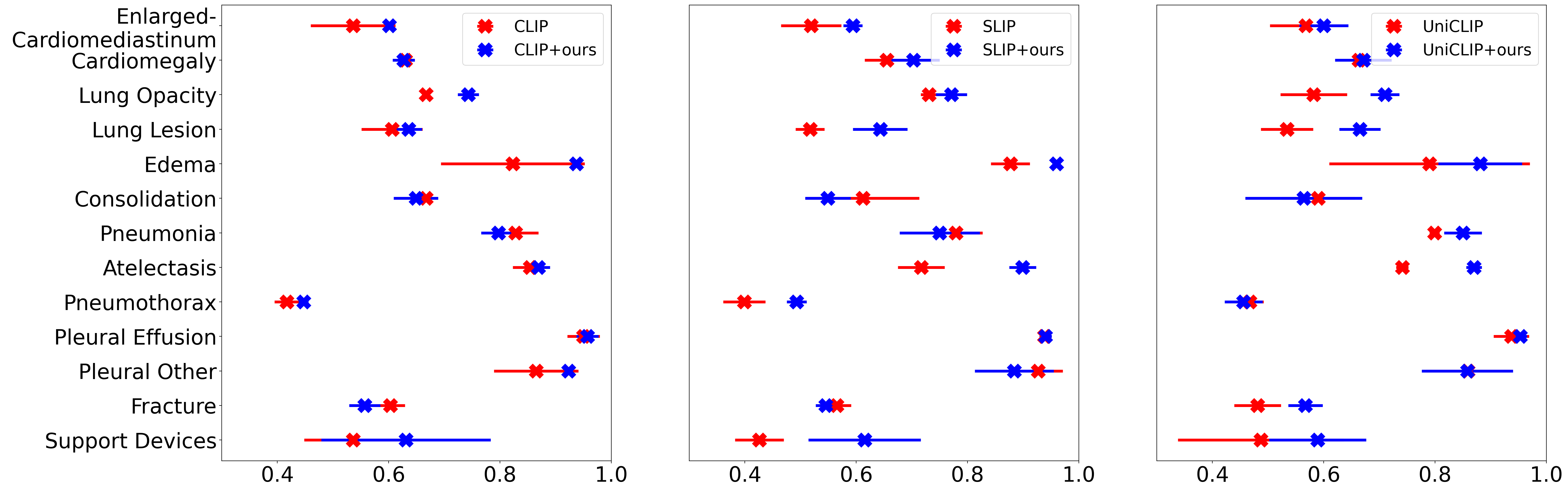
Figure 8: AUROC plot on Open-i testset of each framework

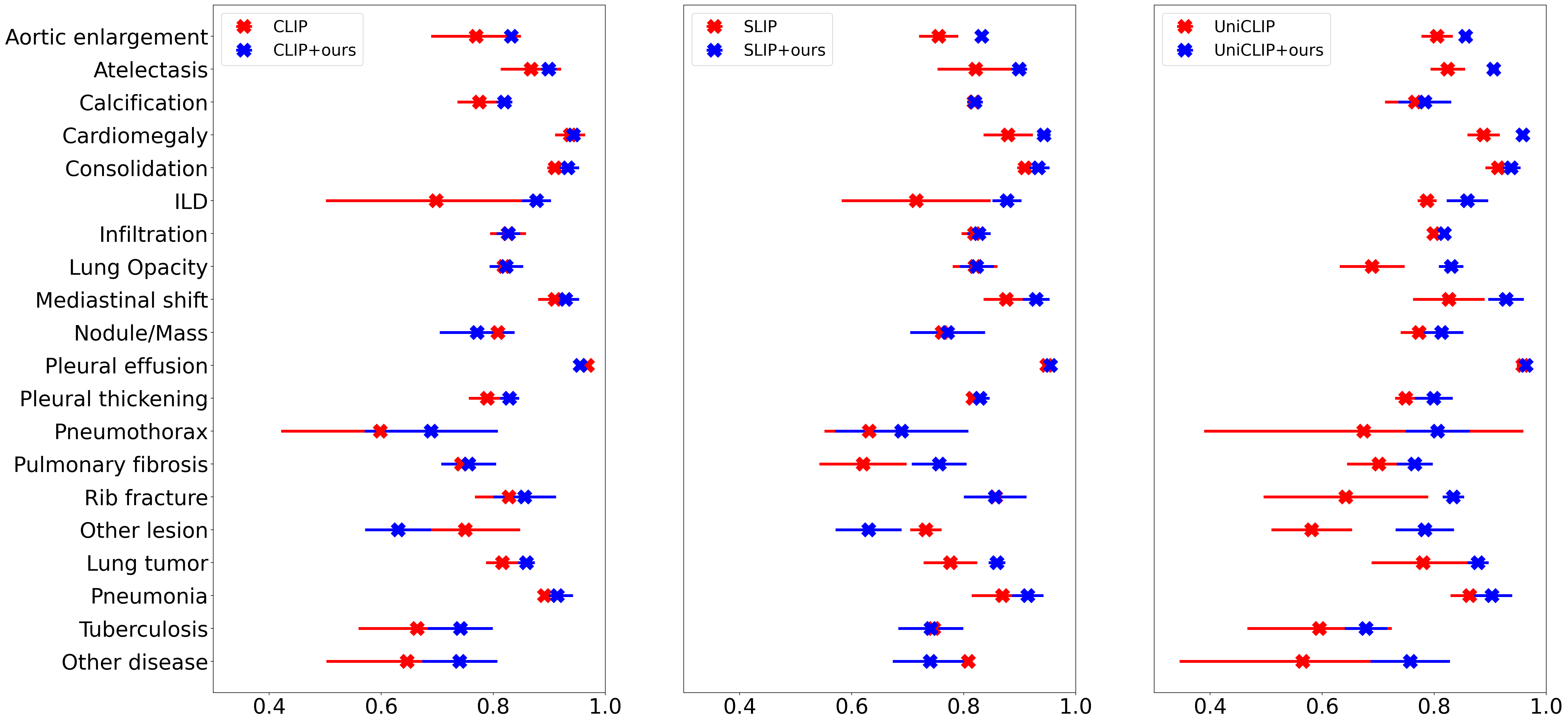
Figure 9: AUROC plot on VinDR-CXR testset of each framework

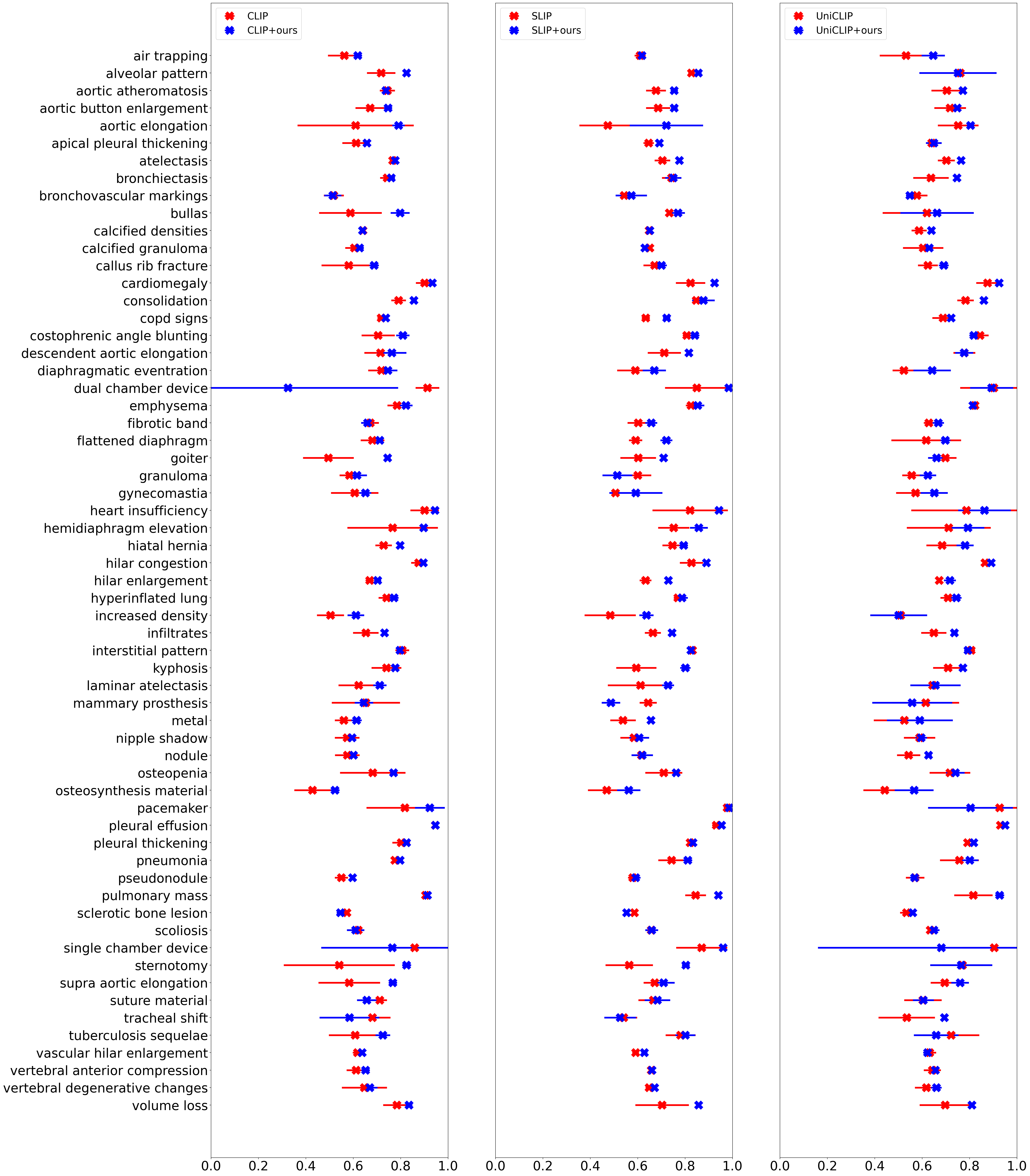
Figure 10: AUROC plot on PadChest testset of each framework

In this section, we provide detailed results for each label on CheXpert, Open-i, VinDR-CXR, and PadChest. All the label information we used is described in  Tab. 7. We provide AUROC performance for all pathologies in each test dataset in Tab. 8, Tab. 9, Tab. 10 and Tab. 11. These results are also plotted in Fig. 7, Fig. 8, Fig. 9, and Fig. 10.

	names
CheXpert [15]	Enlarged Cardiomediastinum, Cardiomegaly, Lung Opacity, Lung Lesion, Edema, Consolidation, Pneumonia, Atelectasis, Pneumothorax, Pleural Effusion, Pleural Other, Fracture, Support Devices
Open-i [9]	Enlarged Cardiomediastinum, Cardiomegaly, Lung Opacity, Lung Lesion, Edema, Consolidation, Pneumonia, Atelectasis, Pneumothorax, Pleural Effusion, Pleural Other, Fracture, Support Devices
PadChest [5]	Air Trapping, Alveolar Pattern, Aortic Atheromatosis, Aortic Button Enlargement, Aortic Elongation, Apical Pleural Thickening, Atelectasis, Bronchiectasis, Bronchovascular Markings, Bullas, Calcified Densities, Calcified Granuloma, Callus Rib Fracture, Cardiomegaly, Consolidation, Copd Signs, Costophrenic Angle Blunting, Descendent Aortic Elongation, Diaphragmatic Eventration, Dual Chamber Device, Emphysema, Fibrotic Band, Flattened Diaphragm, Goiter, Granuloma, Gynecomastia, Heart Insufficiency, Hemidiaphragm Elevation, Hiatal Hernia, Hilar Congestion, Hilar Enlargement, Hyperinflated Lung, Increased Density, Infiltrates, Interstitial Pattern, Kyphosis, Laminar Atelectasis, Mammary Prosthesis, Metal, Nipple Shadow, Nodule, Osteopenia, Osteosynthesis Material, Pacemaker, Pleural Effusion, Pleural Thickening, Pneumonia, Pseudonodule, Pulmonary Mass, Sclerotic Bone Lesion, Scoliosis, Single Chamber Device, Sternotomy, Supra Aortic Elongation, Suture Material, Tracheal Shift, Tuberculosis Sequelae, Vascular Hilar Enlargement, Vertebral Anterior Compression, Vertebral Degenerative Changes, Volume Loss
VinDr-CXR [24]	Aortic enlargement, Atelectasis, Calcification, Cardiomegaly, Consolidation, ILD, Infiltration, Lung Opacity, Mediastinal Shift, Nodule/Mass, Pleural Effusion, Pleural Thickening, Pneumothorax, Pulmonary Fibrosis, Rib Fracture, Other Lesion, Lung Tumor, Pneumonia, Tuberculosis, Other Disease

Table 7: All labels used in this paper.

	CLIP	CLIP w/ ours	SLIP	SLIP w/ ours	UniCLIP	UniCLIP w/ ours	CheXzero	MedCLIP∗
Enlarged Cardiomediastinum	0.883 ± 0.022	0.885 ± 0.016	0.841 ± 0.028	0.862 ± 0.048	0.866 ± 0.008	0.867 ± 0.044	0.893 ± 0.004	0.780
Cardiomegaly	0.876 ± 0.012	0.885 ± 0.014	0.833 ± 0.021	0.895 ± 0.015	0.870 ± 0.014	0.893 ± 0.009	0.880 ± 0.007	0.808
Lung Opacity	0.854 ± 0.033	0.913 ± 0.001	0.882 ± 0.013	0.906 ± 0.011	0.760 ± 0.080	0.857 ± 0.070	0.872 ± 0.008	0.906
Lung Lesion	0.773 ± 0.051	0.675 ± 0.048	0.661 ± 0.061	0.784 ± 0.020	0.728 ± 0.136	0.827 ± 0.149	0.647 ± 0.068	0.630
Edema	0.885 ± 0.010	0.884 ± 0.010	0.868 ± 0.009	0.905 ± 0.002	0.842 ± 0.040	0.892 ± 0.009	0.824 ± 0.019	0.903
Consolidation	0.887 ± 0.023	0.889 ± 0.016	0.811 ± 0.009	0.886 ± 0.020	0.836 ± 0.014	0.894 ± 0.020	0.838 ± 0.007	0.898
Pneumonia	0.770 ± 0.061	0.820 ± 0.037	0.655 ± 0.053	0.854 ± 0.046	0.739 ± 0.076	0.807 ± 0.051	0.723 ± 0.046	0.880
Atelectasis	0.810 ± 0.013	0.860 ± 0.003	0.735 ± 0.049	0.848 ± 0.022	0.799 ± 0.046	0.850 ± 0.013	0.784 ± 0.034	0.839
Pneumothorax	0.643 ± 0.054	0.800 ± 0.007	0.574 ± 0.049	0.641 ± 0.084	0.620 ± 0.241	0.766 ± 0.066	0.579 ± 0.016	0.972
Pleural Effusion	0.891 ± 0.019	0.908 ± 0.010	0.906 ± 0.005	0.886 ± 0.013	0.907 ± 0.010	0.909 ± 0.016	0.894 ± 0.010	0.950
Pleural Other	0.502 ± 0.060	0.537 ± 0.053	0.521 ± 0.065	0.452 ± 0.036	0.638 ± 0.092	0.617 ± 0.040	0.509 ± 0.009	0.653
Fracture	0.529 ± 0.092	0.511 ± 0.042	0.550 ± 0.077	0.499 ± 0.040	0.411 ± 0.096	0.556 ± 0.041	0.416 ± 0.025	0.597
Support Devices	0.716 ± 0.144	0.692 ± 0.119	0.659 ± 0.026	0.706 ± 0.069	0.620 ± 0.162	0.687 ± 0.021	0.694 ± 0.043	0.961

• $\ast$: use label information defined in CheXpert for training

Table 8: Zero-shot classification performance measured by AUROC on three different CLIP-based frameworks on the CheXpert testset (mean ± std).

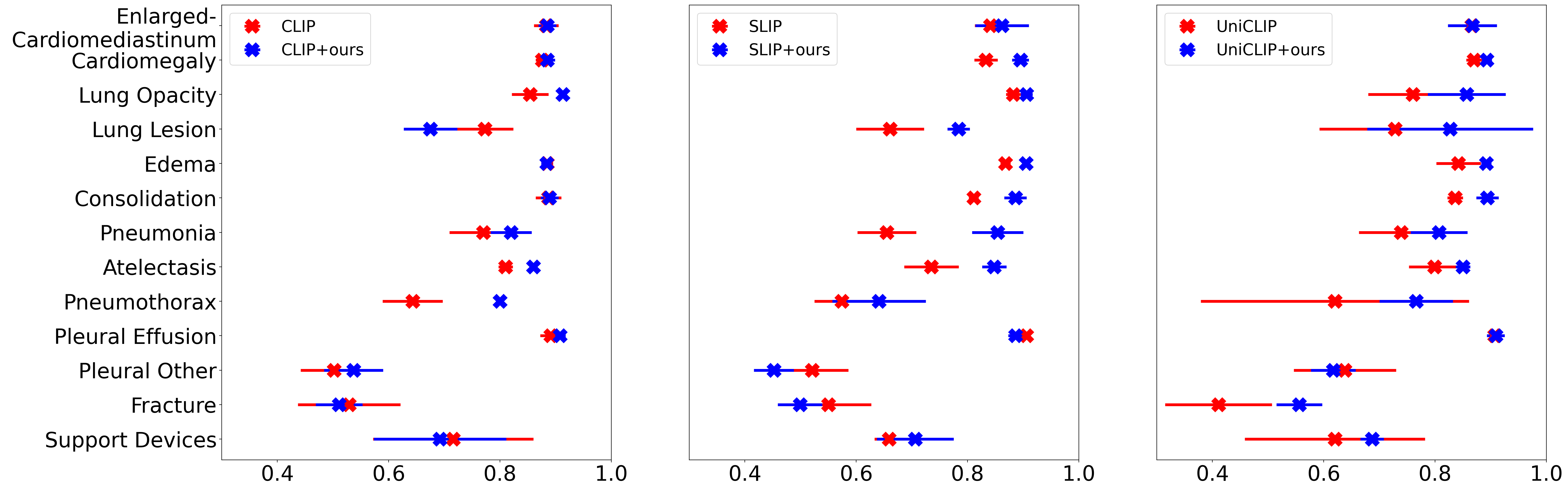
Figure 7: AUROC plot on CheXpert testset of each framework

	CLIP	CLIP w/ ours	SLIP	SLIP w/ ours	UniCLIP	UniCLIP w/ ours	CheXzero	MedCLIP∗
Enlarged Cardiomediastinum	0.536 ± 0.076	0.601 ± 0.005	0.519 ± 0.054	0.594 ± 0.017	0.568 ± 0.065	0.600 ± 0.044	0.580 ± 0.035	0.542
Cardiomegaly	0.630 ± 0.015	0.627 ± 0.020	0.655 ± 0.040	0.703 ± 0.047	0.663 ± 0.010	0.671 ± 0.051	0.637 ± 0.012	0.715
Lung Opacity	0.667 ± 0.007	0.743 ± 0.019	0.731 ± 0.015	0.771 ± 0.028	0.582 ± 0.060	0.710 ± 0.026	0.679 ± 0.026	0.768
Lung Lesion	0.606 ± 0.055	0.636 ± 0.024	0.517 ± 0.026	0.643 ± 0.049	0.534 ± 0.047	0.665 ± 0.037	0.535 ± 0.024	0.581
Edema	0.823 ± 0.129	0.937 ± 0.004	0.877 ± 0.035	0.960 ± 0.007	0.790 ± 0.180	0.881 ± 0.075	0.859 ± 0.065	0.965
Consolidation	0.667 ± 0.020	0.649 ± 0.040	0.612 ± 0.101	0.549 ± 0.041	0.590 ± 0.066	0.564 ± 0.105	0.628 ± 0.040	0.462
Pneumonia	0.828 ± 0.041	0.797 ± 0.031	0.779 ± 0.048	0.750 ± 0.072	0.799 ± 0.009	0.850 ± 0.034	0.785 ± 0.025	0.858
Atelectasis	0.854 ± 0.031	0.869 ± 0.021	0.717 ± 0.042	0.899 ± 0.024	0.741 ± 0.011	0.870 ± 0.014	0.824 ± 0.025	0.898
Pneumothorax	0.417 ± 0.022	0.447 ± 0.009	0.399 ± 0.038	0.493 ± 0.018	0.467 ± 0.025	0.456 ± 0.034	0.416 ± 0.028	0.505
Pleural Effusion	0.950 ± 0.029	0.957 ± 0.020	0.938 ± 0.007	0.940 ± 0.011	0.937 ± 0.032	0.953 ± 0.012	0.904 ± 0.040	0.929
Pleural Other	0.865 ± 0.076	0.923 ± 0.004	0.927 ± 0.044	0.884 ± 0.071	0.859 ± 0.075	0.858 ± 0.082	0.938 ± 0.021	0.898
Fracture	0.603 ± 0.026	0.557 ± 0.028	0.565 ± 0.026	0.545 ± 0.018	0.481 ± 0.042	0.567 ± 0.031	0.567 ± 0.024	0.540
Support Devices	0.536 ± 0.088	0.631 ± 0.152	0.426 ± 0.044	0.615 ± 0.101	0.487 ± 0.149	0.589 ± 0.087	0.538 ± 0.051	0.806

• $\ast$: use label information defined in CheXpert for training

Table 9: Zero-shot classification performance on three different CLIP-based frameworks on the Open-i testset (mean ± std).

	CLIP	CLIP w/ ours	SLIP	SLIP w/ ours	UniCLIP	UniCLIP w/ ours	CheXzero	MedCLIP∗
Aortic Enlargement	0.769 ± 0.080	0.832 ± 0.005	0.755 ± 0.035	0.832 ± 0.005	0.805 ± 0.028	0.856 ± 0.009	0.834 ± 0.020	0.800
Atelectasis	0.867 ± 0.054	0.899 ± 0.014	0.821 ± 0.068	0.899 ± 0.014	0.824 ± 0.031	0.906 ± 0.009	0.785 ± 0.017	0.911
Calcification	0.775 ± 0.039	0.820 ± 0.014	0.818 ± 0.004	0.820 ± 0.014	0.766 ± 0.054	0.783 ± 0.047	0.804 ± 0.042	0.779
Cardiomegaly	0.937 ± 0.027	0.943 ± 0.012	0.879 ± 0.044	0.943 ± 0.012	0.888 ± 0.029	0.958 ± 0.008	0.941 ± 0.014	0.857
Consolidation	0.910 ± 0.014	0.933 ± 0.020	0.909 ± 0.014	0.933 ± 0.020	0.914 ± 0.023	0.937 ± 0.017	0.823 ± 0.035	0.954
ILD	0.698 ± 0.197	0.877 ± 0.026	0.715 ± 0.133	0.877 ± 0.026	0.787 ± 0.017	0.859 ± 0.037	0.733 ± 0.075	0.735
Infiltration	0.826 ± 0.032	0.827 ± 0.021	0.819 ± 0.023	0.827 ± 0.021	0.799 ± 0.007	0.818 ± 0.008	0.780 ± 0.008	0.877
Lung Opacity	0.819 ± 0.009	0.823 ± 0.030	0.820 ± 0.040	0.823 ± 0.030	0.689 ± 0.058	0.830 ± 0.022	0.765 ± 0.040	0.861
Mediastinal Shift	0.910 ± 0.030	0.929 ± 0.024	0.876 ± 0.041	0.929 ± 0.024	0.826 ± 0.064	0.928 ± 0.032	0.790 ± 0.133	0.855
Nodule/Mass	0.808 ± 0.025	0.771 ± 0.067	0.761 ± 0.043	0.771 ± 0.067	0.773 ± 0.033	0.813 ± 0.039	0.702 ± 0.133	0.850
Pleural Effusion	0.968 ± 0.005	0.955 ± 0.004	0.948 ± 0.008	0.955 ± 0.004	0.958 ± 0.011	0.964 ± 0.004	0.911 ± 0.036	0.983
Pleural Thickening	0.789 ± 0.033	0.829 ± 0.017	0.816 ± 0.009	0.829 ± 0.017	0.749 ± 0.019	0.799 ± 0.034	0.779 ± 0.018	0.829
Pneumothorax	0.598 ± 0.177	0.689 ± 0.119	0.631 ± 0.080	0.689 ± 0.119	0.674 ± 0.285	0.806 ± 0.057	0.637 ± 0.039	0.969
Pulmonary Fibrosis	0.743 ± 0.014	0.756 ± 0.049	0.620 ± 0.078	0.756 ± 0.049	0.701 ± 0.057	0.765 ± 0.032	0.714 ± 0.090	0.822
Rib Fracture	0.828 ± 0.061	0.856 ± 0.056	0.857 ± 0.031	0.856 ± 0.056	0.642 ± 0.147	0.834 ± 0.019	0.861 ± 0.022	0.809
Other Lesion	0.750 ± 0.098	0.630 ± 0.059	0.732 ± 0.028	0.630 ± 0.059	0.581 ± 0.072	0.783 ± 0.052	0.632 ± 0.162	0.525
Lung Tumor	0.816 ± 0.029	0.859 ± 0.015	0.776 ± 0.048	0.859 ± 0.015	0.780 ± 0.092	0.878 ± 0.019	0.779 ± 0.032	0.926
Pneumonia	0.891 ± 0.003	0.914 ± 0.028	0.869 ± 0.055	0.914 ± 0.028	0.863 ± 0.034	0.903 ± 0.036	0.836 ± 0.033	0.933
Tuberculosis	0.664 ± 0.105	0.741 ± 0.058	0.746 ± 0.036	0.741 ± 0.058	0.595 ± 0.129	0.678 ± 0.038	0.643 ± 0.038	0.717
Other Disease	0.646 ± 0.144	0.740 ± 0.067	0.808 ± 0.003	0.740 ± 0.067	0.565 ± 0.220	0.757 ± 0.071	0.662 ± 0.160	0.584

• $\ast$: use label information defined in CheXpert for training

Table 10: Zero-shot classification performance on three different CLIP-based frameworks on the VinDR-CXR testset (mean ± std).

	CLIP	CLIP w/ ours	SLIP	SLIP w/ ours	UniCLIP	UniCLIP w/ ours	CheXzero	MedCLIP∗
Air Trapping	0.562 ± 0.069	0.619 ± 0.018	0.610 ± 0.023	0.618 ± 0.009	0.532 ± 0.111	0.647 ± 0.049	0.596 ± 0.047	0.598
Alveolar Pattern	0.718 ± 0.060	0.825 ± 0.012	0.827 ± 0.014	0.856 ± 0.013	0.761 ± 0.045	0.751 ± 0.163	0.751 ± 0.065	0.840
Aortic Atheromatosis	0.744 ± 0.032	0.738 ± 0.008	0.677 ± 0.042	0.754 ± 0.015	0.704 ± 0.065	0.772 ± 0.012	0.750 ± 0.011	0.754
Aortic Button Enlargement	0.671 ± 0.062	0.747 ± 0.017	0.686 ± 0.051	0.754 ± 0.014	0.718 ± 0.067	0.748 ± 0.006	0.721 ± 0.027	0.763
Aortic Elongation	0.610 ± 0.245	0.791 ± 0.026	0.474 ± 0.120	0.721 ± 0.155	0.752 ± 0.086	0.804 ± 0.016	0.765 ± 0.070	0.707
Apical Pleural Thickening	0.612 ± 0.058	0.658 ± 0.001	0.646 ± 0.022	0.691 ± 0.008	0.640 ± 0.008	0.649 ± 0.033	0.628 ± 0.025	0.637
Atelectasis	0.766 ± 0.012	0.777 ± 0.010	0.704 ± 0.033	0.776 ± 0.005	0.702 ± 0.036	0.764 ± 0.003	0.712 ± 0.017	0.798
Bronchiectasis	0.743 ± 0.030	0.760 ± 0.016	0.743 ± 0.041	0.750 ± 0.034	0.637 ± 0.075	0.747 ± 0.009	0.684 ± 0.015	0.760
Bronchovascular Markings	0.518 ± 0.042	0.514 ± 0.036	0.543 ± 0.015	0.573 ± 0.066	0.578 ± 0.044	0.548 ± 0.016	0.518 ± 0.020	0.594
Bullas	0.588 ± 0.132	0.798 ± 0.040	0.733 ± 0.007	0.770 ± 0.029	0.620 ± 0.187	0.663 ± 0.155	0.744 ± 0.046	0.781
Calcified Densities	0.641 ± 0.009	0.639 ± 0.011	0.648 ± 0.004	0.651 ± 0.007	0.587 ± 0.032	0.639 ± 0.012	0.620 ± 0.022	0.635
Calcified Granuloma	0.605 ± 0.039	0.627 ± 0.018	0.651 ± 0.006	0.630 ± 0.010	0.604 ± 0.085	0.630 ± 0.014	0.622 ± 0.013	0.610
Callus Rib Fracture	0.581 ± 0.115	0.688 ± 0.020	0.671 ± 0.047	0.700 ± 0.023	0.624 ± 0.042	0.691 ± 0.021	0.681 ± 0.022	0.733
Cardiomegaly	0.901 ± 0.037	0.934 ± 0.003	0.823 ± 0.062	0.924 ± 0.009	0.876 ± 0.048	0.925 ± 0.007	0.921 ± 0.007	0.822
Consolidation	0.791 ± 0.031	0.856 ± 0.012	0.847 ± 0.009	0.877 ± 0.048	0.783 ± 0.035	0.860 ± 0.005	0.793 ± 0.011	0.941
COPD Signs	0.718 ± 0.016	0.737 ± 0.010	0.634 ± 0.017	0.722 ± 0.015	0.688 ± 0.045	0.722 ± 0.009	0.686 ± 0.030	0.697
Costophrenic Angle Blunting	0.705 ± 0.070	0.809 ± 0.028	0.807 ± 0.017	0.841 ± 0.019	0.844 ± 0.036	0.818 ± 0.019	0.769 ± 0.011	0.831
Descendent Aortic Elongation	0.715 ± 0.068	0.763 ± 0.061	0.712 ± 0.070	0.816 ± 0.008	0.778 ± 0.046	0.777 ± 0.038	0.726 ± 0.021	0.482
Diaphragmatic Eventration	0.719 ± 0.056	0.746 ± 0.040	0.590 ± 0.077	0.670 ± 0.049	0.523 ± 0.048	0.642 ± 0.079	0.666 ± 0.099	0.622
Dual Chamber Device	0.913 ± 0.050	0.325 ± 0.464	0.849 ± 0.134	0.984 ± 0.013	0.902 ± 0.142	0.893 ± 0.091	0.920 ± 0.058	0.995
Emphysema	0.785 ± 0.041	0.822 ± 0.028	0.825 ± 0.022	0.853 ± 0.028	0.823 ± 0.013	0.814 ± 0.011	0.815 ± 0.009	0.654
Fibrotic Band	0.672 ± 0.036	0.660 ± 0.027	0.602 ± 0.045	0.657 ± 0.025	0.628 ± 0.021	0.668 ± 0.024	0.604 ± 0.074	0.670
Flattened Diaphragm	0.681 ± 0.050	0.712 ± 0.014	0.591 ± 0.028	0.721 ± 0.025	0.617 ± 0.147	0.698 ± 0.021	0.618 ± 0.020	0.689
Goiter	0.495 ± 0.107	0.745 ± 0.013	0.602 ± 0.075	0.709 ± 0.009	0.698 ± 0.047	0.661 ± 0.036	0.665 ± 0.071	0.667
Granuloma	0.584 ± 0.042	0.616 ± 0.042	0.600 ± 0.057	0.514 ± 0.063	0.556 ± 0.040	0.624 ± 0.035	0.611 ± 0.021	0.574
Gynecomastia	0.606 ± 0.100	0.651 ± 0.025	0.506 ± 0.021	0.592 ± 0.112	0.572 ± 0.082	0.651 ± 0.057	0.660 ± 0.020	0.604
Heart Insufficiency	0.901 ± 0.060	0.945 ± 0.004	0.821 ± 0.159	0.943 ± 0.008	0.787 ± 0.233	0.863 ± 0.111	0.939 ± 0.002	0.958
Hemidiaphragm Elevation	0.766 ± 0.191	0.897 ± 0.006	0.752 ± 0.066	0.858 ± 0.038	0.712 ± 0.177	0.793 ± 0.069	0.835 ± 0.021	0.751
Hiatal Hernia	0.728 ± 0.035	0.798 ± 0.006	0.747 ± 0.043	0.794 ± 0.018	0.684 ± 0.066	0.781 ± 0.036	0.758 ± 0.011	0.727
Hilar Congestion	0.876 ± 0.032	0.896 ± 0.007	0.827 ± 0.049	0.890 ± 0.006	0.865 ± 0.003	0.891 ± 0.006	0.896 ± 0.005	0.797
Hilar Enlargement	0.669 ± 0.017	0.703 ± 0.015	0.633 ± 0.025	0.729 ± 0.004	0.672 ± 0.005	0.717 ± 0.025	0.659 ± 0.049	0.679
Hyperinflated Lung	0.741 ± 0.034	0.772 ± 0.019	0.769 ± 0.017	0.787 ± 0.024	0.709 ± 0.032	0.744 ± 0.022	0.752 ± 0.012	0.715
Increased Density	0.504 ± 0.057	0.611 ± 0.035	0.484 ± 0.108	0.637 ± 0.030	0.509 ± 0.051	0.501 ± 0.120	0.546 ± 0.040	0.694
Infiltrates	0.653 ± 0.054	0.732 ± 0.010	0.664 ± 0.034	0.745 ± 0.012	0.649 ± 0.053	0.736 ± 0.013	0.674 ± 0.017	0.768
Interstitial Pattern	0.807 ± 0.029	0.797 ± 0.014	0.831 ± 0.005	0.824 ± 0.009	0.807 ± 0.016	0.793 ± 0.016	0.739 ± 0.015	0.706
Kyphosis	0.740 ± 0.063	0.777 ± 0.010	0.594 ± 0.085	0.801 ± 0.022	0.709 ± 0.063	0.772 ± 0.011	0.743 ± 0.023	0.765
Laminar Atelectasis	0.623 ± 0.085	0.712 ± 0.028	0.612 ± 0.138	0.728 ± 0.025	0.644 ± 0.069	0.656 ± 0.106	0.675 ± 0.013	0.820
Mammary Prosthesis	0.653 ± 0.144	0.645 ± 0.039	0.644 ± 0.036	0.487 ± 0.039	0.615 ± 0.141	0.558 ± 0.169	0.671 ± 0.141	0.753
Metal	0.560 ± 0.038	0.614 ± 0.022	0.538 ± 0.054	0.656 ± 0.010	0.525 ± 0.129	0.590 ± 0.139	0.594 ± 0.068	0.692
Nipple Shadow	0.574 ± 0.052	0.595 ± 0.006	0.584 ± 0.057	0.606 ± 0.042	0.589 ± 0.066	0.596 ± 0.024	0.530 ± 0.032	0.559
Nodule	0.575 ± 0.052	0.601 ± 0.009	0.616 ± 0.020	0.619 ± 0.045	0.543 ± 0.049	0.627 ± 0.013	0.587 ± 0.022	0.648
Osteopenia	0.682 ± 0.138	0.770 ± 0.014	0.710 ± 0.078	0.762 ± 0.008	0.717 ± 0.086	0.740 ± 0.039	0.732 ± 0.021	0.681
Osteosynthesis Material	0.428 ± 0.077	0.523 ± 0.019	0.469 ± 0.079	0.562 ± 0.049	0.442 ± 0.090	0.566 ± 0.082	0.498 ± 0.073	0.694
Pacemaker	0.818 ± 0.162	0.923 ± 0.063	0.977 ± 0.014	0.986 ± 0.007	0.927 ± 0.073	0.804 ± 0.179	0.929 ± 0.011	0.997
Pleural Effusion	0.946 ± 0.003	0.947 ± 0.008	0.931 ± 0.017	0.954 ± 0.003	0.930 ± 0.011	0.950 ± 0.003	0.918 ± 0.016	0.954
Pleural Thickening	0.802 ± 0.037	0.825 ± 0.006	0.821 ± 0.008	0.833 ± 0.009	0.791 ± 0.010	0.818 ± 0.011	0.780 ± 0.025	0.842
Pneumonia	0.775 ± 0.010	0.798 ± 0.012	0.743 ± 0.056	0.811 ± 0.019	0.757 ± 0.082	0.801 ± 0.036	0.741 ± 0.016	0.765
Pseudonodule	0.550 ± 0.028	0.597 ± 0.002	0.579 ± 0.020	0.591 ± 0.021	0.570 ± 0.039	0.568 ± 0.020	0.558 ± 0.006	0.600
Pulmonary Mass	0.905 ± 0.010	0.913 ± 0.009	0.844 ± 0.044	0.940 ± 0.006	0.816 ± 0.081	0.927 ± 0.019	0.875 ± 0.034	0.927
Sclerotic Bone Lesion	0.573 ± 0.011	0.546 ± 0.016	0.586 ± 0.008	0.553 ± 0.007	0.534 ± 0.027	0.560 ± 0.008	0.583 ± 0.006	0.578
Scoliosis	0.621 ± 0.024	0.610 ± 0.037	0.657 ± 0.005	0.659 ± 0.027	0.634 ± 0.010	0.649 ± 0.024	0.619 ± 0.025	0.612
Single Chamber Device	0.859 ± 0.097	0.765 ± 0.300	0.870 ± 0.108	0.960 ± 0.011	0.904 ± 0.135	0.681 ± 0.521	0.673 ± 0.528	0.990
Sternotomy	0.541 ± 0.234	0.825 ± 0.019	0.564 ± 0.100	0.803 ± 0.016	0.770 ± 0.086	0.765 ± 0.131	0.742 ± 0.066	0.843
Supra Aortic Elongation	0.583 ± 0.130	0.767 ± 0.018	0.672 ± 0.047	0.709 ± 0.047	0.695 ± 0.059	0.760 ± 0.037	0.735 ± 0.060	0.737
Suture Material	0.712 ± 0.030	0.657 ± 0.041	0.666 ± 0.063	0.683 ± 0.054	0.603 ± 0.079	0.605 ± 0.044	0.653 ± 0.039	0.708
Tracheal Shift	0.681 ± 0.076	0.584 ± 0.126	0.541 ± 0.057	0.526 ± 0.067	0.535 ± 0.119	0.694 ± 0.001	0.595 ± 0.077	0.665
Tuberculosis Sequelae	0.608 ± 0.111	0.725 ± 0.031	0.781 ± 0.063	0.801 ± 0.042	0.722 ± 0.119	0.659 ± 0.094	0.653 ± 0.028	0.661
Vascular Hilar Enlargement	0.618 ± 0.020	0.638 ± 0.010	0.591 ± 0.014	0.628 ± 0.013	0.632 ± 0.027	0.623 ± 0.019	0.644 ± 0.018	0.492
Vertebral Anterior Compression	0.612 ± 0.040	0.652 ± 0.018	0.657 ± 0.010	0.660 ± 0.011	0.643 ± 0.036	0.656 ± 0.012	0.644 ± 0.017	0.638
Vertebral Degenerative Changes	0.647 ± 0.095	0.670 ± 0.032	0.648 ± 0.015	0.671 ± 0.011	0.618 ± 0.049	0.660 ± 0.022	0.653 ± 0.049	0.661
Volume Loss	0.784 ± 0.058	0.835 ± 0.014	0.703 ± 0.113	0.857 ± 0.011	0.697 ± 0.108	0.810 ± 0.010	0.748 ± 0.023	0.852

• $\ast$: use label information defined in CheXpert for training

Table 11: Zero-shot classification performance on three different CLIP-based frameworks on the PadChest testset (mean ± std).

References

- [1] Mahdi Abdollahi et al. Ontology-guided data augmentation for medical document classification. In Artificial Intelligence in Medicine, 2020.
- [2] Open Ai. https://github.com/openai/clip.
- [3] Shekoofeh Azizi, Basil Mustafa, Fiona Ryan, Zachary Beaver, Jan Freyberg, Jonathan Deaton, Aaron Loh, Alan Karthikesalingam, Simon Kornblith, Ting Chen, et al. Big self-supervised models advance medical image classification. In Proceedings of the IEEE/CVF International Conference on Computer Vision, pages 3478–3488, 2021.
- [4] Markus Bayer et al. A survey on data augmentation for text classification. ACM Computing Surveys, 2022.
- [5] Aurelia Bustos, Antonio Pertusa, Jose-Maria Salinas, and Maria de la Iglesia-Vayá. Padchest: A large chest x-ray image dataset with multi-label annotated reports. Medical image analysis, 66:101797, 2020.
- [6] Ting Chen, Simon Kornblith, Mohammad Norouzi, and Geoffrey Hinton. A simple framework for contrastive learning of visual representations. In International conference on machine learning, pages 1597–1607. PMLR, 2020.
- [7] Hyunsoo Cho, Jinseok Seol, and Sang-goo Lee. Masked contrastive learning for anomaly detection. In IJCAI, 2021.
- [8] Dina Demner-Fushman, Sameer Antani, Matthew Simpson, and George R Thoma. Design and development of a multimodal biomedical information retrieval system. Journal of Computing Science and Engineering, 6(2):168–177, 2012.
- [9] Dina Demner-Fushman, Marc Kohli, Marc Rosenman, Sonya Shooshan, Laritza Rodriguez, Sameer Antani, George Thoma, and Clement Mcdonald. Preparing a collection of radiology examinations for distribution and retrieval. Journal of the American Medical Informatics Association : JAMIA, 23, 07 2015.
- [10] Jacob Devlin, Ming-Wei Chang, Kenton Lee, and Kristina Toutanova. BERT: Pre-training of deep bidirectional transformers for language understanding. In Proceedings of the 2019 Conference of the North American Chapter of the Association for Computational Linguistics: Human Language Technologies, Volume 1 (Long and Short Papers), 2019.
- [11] Alexey Dosovitskiy, Lucas Beyer, Alexander Kolesnikov, Dirk Weissenborn, Xiaohua Zhai, Thomas Unterthiner, Mostafa Dehghani, Matthias Minderer, Georg Heigold, Sylvain Gelly, Jakob Uszkoreit, and Neil Houlsby. An image is worth 16x16 words: Transformers for image recognition at scale. In International Conference on Learning Representations, 2021.
- [12] Andre Esteva, Brett Kuprel, Roberto A Novoa, Justin Ko, Susan M Swetter, Helen M Blau, and Sebastian Thrun. Dermatologist-level classification of skin cancer with deep neural networks. nature, 542(7639):115–118, 2017.
- [13] Varun Gulshan, Lily Peng, Marc Coram, Martin C Stumpe, Derek Wu, Arunachalam Narayanaswamy, Subhashini Venugopalan, Kasumi Widner, Tom Madams, Jorge Cuadros, Ramasamy Kim, Rajiv Raman, Philip Q Nelson, Jessica Mega, and Dale Webster. Development and validation of a deep learning algorithm for detection of diabetic retinopathy in retinal fundus photographs. JAMA, 2016.
- [14] Shih-Cheng Huang, Liyue Shen, Matthew P. Lungren, and Serena Yeung. Gloria: A multimodal global-local representation learning framework for label-efficient medical image recognition. In 2021 IEEE/CVF International Conference on Computer Vision (ICCV), pages 3922–3931, 2021.
- [15] Jeremy Irvin, Pranav Rajpurkar, Michael Ko, Yifan Yu, Silviana Ciurea-Ilcus, Chris Chute, Henrik Marklund, Behzad Haghgoo, Robyn Ball, Katie Shpanskaya, et al. Chexpert: A large chest radiograph dataset with uncertainty labels and expert comparison. In Proceedings of the AAAI conference on artificial intelligence, volume 33, pages 590–597, 2019.
- [16] Alistair EW Johnson, Tom J Pollard, Seth J Berkowitz, Nathaniel R Greenbaum, Matthew P Lungren, Chih-ying Deng, Roger G Mark, and Steven Horng. Mimic-cxr, a de-identified publicly available database of chest radiographs with free-text reports. Scientific data, 6(1):1–8, 2019.
- [17] Alexander Ke, William Ellsworth, Oishi Banerjee, Andrew Y Ng, and Pranav Rajpurkar. Chextransfer: performance and parameter efficiency of imagenet models for chest x-ray interpretation. In Proceedings of the Conference on Health, Inference, and Learning, pages 116–124, 2021.
- [18] Diederik P. Kingma and Jimmy Ba. Adam: A method for stochastic optimization. In ICLR, 2015.
- [19] Jonathan Krause, Varun Gulshan, Ehsan Rahimy, Peter Karth, Kasumi Widner, Greg S Corrado, Lily Peng, and Dale R Webster. Grader variability and the importance of reference standards for evaluating machine learning models for diabetic retinopathy. Ophthalmology, 125(8):1264–1272, 2018.
- [20] Janghyeon Lee, Jongsuk Kim, Hyounguk Shon, Bumsoo Kim, Seung Hwan Kim, Honglak Lee, and Junmo Kim. Uniclip: Unified framework for contrastive language-image pre-training. arXiv preprint arXiv:2209.13430, 2022.
- [21] Ilya Loshchilov and Frank Hutter. Sgdr: Stochastic gradient descent with warm restarts. arXiv preprint arXiv:1608.03983, 2016.
- [22] Norman Mu, Alexander Kirillov, David Wagner, and Saining Xie. Slip: Self-supervision meets language-image pre-training. arXiv preprint arXiv:2112.12750, 2021.
- [23] Basil Mustafa, Aaron Loh, Jan Freyberg, Patricia MacWilliams, Megan Wilson, Scott Mayer McKinney, Marcin Sieniek, Jim Winkens, Yuan Liu, Peggy Bui, et al. Supervised transfer learning at scale for medical imaging. arXiv preprint arXiv:2101.05913, 2021.
- [24] Ha Q Nguyen, Khanh Lam, Linh T Le, Hieu H Pham, Dat Q Tran, Dung B Nguyen, Dung D Le, Chi M Pham, Hang TT Tong, Diep H Dinh, et al. Vindr-cxr: An open dataset of chest x-rays with radiologist’s annotations. Scientific Data, 9(1):1–7, 2022.
- [25] Aaron van den Oord, Yazhe Li, and Oriol Vinyals. Representation learning with contrastive predictive coding. arXiv preprint arXiv:1807.03748, 2018.
- [26] Adam Paszke, Sam Gross, Francisco Massa, Adam Lerer, James Bradbury, Gregory Chanan, Trevor Killeen, Zeming Lin, Natalia Gimelshein, Luca Antiga, Alban Desmaison, Andreas Kopf, Edward Yang, Zachary DeVito, Martin Raison, Alykhan Tejani, Sasank Chilamkurthy, Benoit Steiner, Lu Fang, Junjie Bai, and Soumith Chintala. Pytorch: An imperative style, high-performance deep learning library. In NeurIPS. 2019.
- [27] Alec Radford, Jong Wook Kim, Chris Hallacy, Aditya Ramesh, Gabriel Goh, Sandhini Agarwal, Girish Sastry, Amanda Askell, Pamela Mishkin, Jack Clark, et al. Learning transferable visual models from natural language supervision. In International Conference on Machine Learning, pages 8748–8763. PMLR, 2021.
- [28] Aditya Ramesh, Mikhail Pavlov, Gabriel Goh, Scott Gray, Chelsea Voss, Alec Radford, Mark Chen, and Ilya Sutskever. Zero-shot text-to-image generation. In International Conference on Machine Learning, pages 8821–8831. PMLR, 2021.
- [29] Bart Thomee, David A. Shamma, Gerald Friedland, Benjamin Elizalde, Karl Ni, Douglas Poland, Damian Borth, and Li-Jia Li. YFCC100M: The new data in multimedia research. Communications of the ACM, 59(2):64–73, 2016.
- [30] Ekin Tiu, Ellie Talius, Pujan Patel, Curtis P Langlotz, Andrew Y Ng, and Pranav Rajpurkar. Expert-level detection of pathologies from unannotated chest x-ray images via self-supervised learning. Nature Biomedical Engineering, pages 1–8, 2022.
- [31] Zifeng Wang, Zhenbang Wu, Dinesh Agarwal, and Jimeng Sun. Medclip: Contrastive learning from unpaired medical images and text. In EMNLP, 2022.
- [32] Mike Wu et al. Conditional negative sampling for contrastive learning of visual representations. arXiv, 2020.
- [33] Jiahao Xie et al. Delving into inter-image invariance for unsupervised visual representations. IJCV, 2022.
- [34] Yuhao Zhang, Hang Jiang, Yasuhide Miura, Christopher D Manning, and Curtis P Langlotz. Contrastive learning of medical visual representations from paired images and text. arXiv preprint arXiv:2010.00747, 2020.