Safety Correction from Baseline: Towards the Risk-aware Policy in Robotics via Dual-agent Reinforcement Learning

Abstract

Learning a risk-aware policy is essential but rather challenging in unstructured robotic tasks. Safe reinforcement learning methods open up new possibilities to tackle this problem. However, the conservative policy updates make it intractable to achieve sufficient exploration and desirable performance in complex, sample-expensive environments. In this paper, we propose a dual-agent safe reinforcement learning strategy consisting of a baseline and a safe agent. Such a decoupled framework enables high flexibility, data efficiency and risk-awareness for RL-based control. Concretely, the baseline agent is responsible for maximizing rewards under standard RL settings. Thus, it is compatible with off-the-shelf training techniques of unconstrained optimization, exploration and exploitation. On the other hand, the safe agent mimics the baseline agent for policy improvement and learns to fulfill safety constraints via off-policy RL tuning. In contrast to training from scratch, safe policy correction requires significantly fewer interactions to obtain a near-optimal policy. The dual policies can be optimized synchronously via a shared replay buffer, or leveraging the pre-trained model or the non-learning-based controller as a fixed baseline agent. Experimental results show that our approach can learn feasible skills without prior knowledge as well as deriving risk-averse counterparts from pre-trained unsafe policies. The proposed method outperforms the state-of-the-art safe RL algorithms on difficult robot locomotion and manipulation tasks with respect to both safety constraint satisfaction and sample efficiency.

I INTRODUCTION

Learning-based methods have achieved significant success in many long-standing, difficult robotic tasks [1, 2, 3]. These advances also raise concerns about the safety of autonomous agents in practical applications: It makes sense to maximize total rewards in the context of a specific task, but is very likely to cause unexpected side-effects to the surroundings [4]. In this paper, we focus on the topic of learning “safety” in order to obtain a stationary policy that can finish the original task and deliberately avoid the risks in the environment, which is distinguished from learning “safely”. This problem used to be solved with robust model predictive control [5], Gaussian process regression [6], etc. Safe reinforcement learning (Safe RL) opens up new possibilities for risk-aware policy optimization and continues to gain traction in recent literature [7].

Safe RL aims to maximize cumulative rewards under the precondition that all the given safety constraints are satisfied. However, it is cumbersome to solve such a constrained sequential decision-making problem in a large parametric space, because most of the existing algorithms are sample inefficient due to the on-policy episodic cost evaluation [8] and conservative policy updates [9]. Even worse, many off-the-shelf training techniques in standard RL are less studied in this scope and do not necessarily work when considering the safety constraints. Consequently, directly applying safe RL to robotic tasks is intractable and usually stuck in a dilemma: The agent needs adequate experiences by trial-and-error to master complex skills, but the safe RL algorithm often limits its exploration within safety-proven behaviors, and the poor data efficiency also makes it impractical on risky, sample-expensive robot learning scenarios.

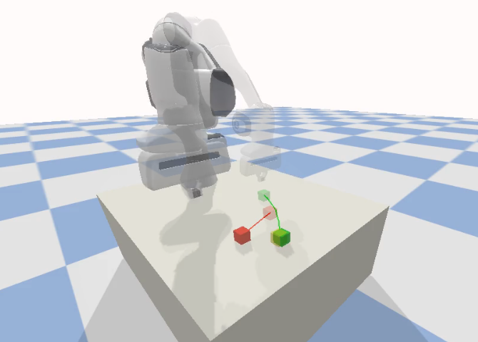
(a) Rollout of Baseline Policy

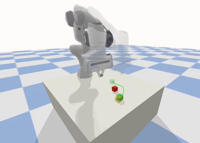
(b) Rollout of Safe Policy

Figure 1: Illustration of the risk-aware policy correction. The robotic arm is required to push the green cube to the destination in the yellow shadow. The baseline policy will move the object along the shortest path, regardless of the obstacle in its way. The safe policy will correct the trajectory slightly to a curve to avoid potential risks instead.

As the example of safe manipulation in Fig. 1, we notice that in most robot learning tasks, the safe policy (considering safety constraints) is similar to the baseline policy (ignoring safety constraints) on the general trend, but with modified actions or trajectories in a few dangerous situations. Motivated by that, we propose a dual-agent algorithm as the alternative for previous safe RL to tackle the above issues in robotic tasks. Concretely, one agent (i.e., the baseline agent) explores the environment and only aims to maximize cumulative rewards. The other (i.e., the safe agent) learns to satisfy given constraints while mimicking the former via online imitation learning to obtain basic skills quickly.

From the perspective of optimization, separating the optimization objective and the constraint can degrade the difficulty of obtaining a feasible solution. We summarize the strengths of the proposed decoupled framework as four-fold: (1) The baseline policy learning is an independent and unconstrained RL task, where most of the training techniques and exploration strategies are available. (2) The difficulty of finding a near-optimal safe policy is reduced due to the online behavior cloning at the early stage and the synchronous constrained RL tuning. (3) The baseline policy guides the safe policy correction and can be in any form. Thus, it is especially pragmatic when we already have pre-trained models or non-learning-based controllers without specific safety considerations, which are common and well-studied in many standard robotic tasks. (4) When it comes to new risky environments, we can execute the safe policy correction with the baseline policy frozen. This significantly increases the sample efficiency compared to training from scratch.

To demonstrate the efficacy of our approach, we design and conduct experiments on different safe robot learning tasks. For the quadruped robot locomotion task, the baseline policy learning and safe policy correction are performed simultaneously without any prior knowledge. For the robotic arm manipulation task, the safe policy is corrected based on a fixed baseline policy which is pre-trained with Hindsight Experience Replay (HER) [10] technique. The empirical results show that our approach can find a near-optimal policy through very limited interactions and outperforms the state-of-the-art safe RL algorithms with respect to safety constraint satisfaction and reward improvement.

II RELATED WORK

II-A Safe Reinforcement Learning

The safety problem in reinforcement learning has become a research hot spot in recent years [11]. In most works, it is regarded as a constrained RL problem, where the agent receives additional cost signals and learns to satisfy the cost constraints. A popular way is leveraging Lagrangian duality for hard constraints [12], but it is rather data inefficient and sensitive to Lagrangian multipliers. As an alternative, Constrained Policy Optimization (CPO) [9] directly searches the feasible policy in the trust-region and guarantees a monotonic performance improvement while satisfying constraints by solving an approximated quadratic optimization problem. Unfortunately, this method suffers from approximation errors and heavy computational burdens for Hessian Matrix inversion, making it incompetent for complex tasks. Another approach is to correct the action at each step by projecting it onto a feasible space. It can be implemented by adding a safety layer [13] or solving a quadratic programming problem [14]. In contrast to training safe policies from scratch, it is much easier to obtain an unconstrained baseline policy and locally modifies it for safety.

II-B Reinforcement Learning from Demonstration

Since we use the baseline policy as guidance, the study of Reinforcement Learning from Demonstration (RLfD) is also related to our work. Previous methods [15, 16, 17] try to combine behavioral cloning (BC) with RL to speed up training and improve the exploration efficiency. Extensive studies [18, 19, 20] show that even imperfect demonstrations are allowed to guide the policy improvement. The key principle of those methods is to find an optimal policy that maximizes the return while mimicking the expert strategy, where a combined loss function of RL and supervised learning is widely used for training. However, such a setting is sensitive to the initialization of the weight coefficients and the learning rate. Furthermore, [21] considers safety issues in RLfD to avoid undesirable behaviors, where Lagrangian relaxation is applied to solve the constrained optimization problem.

II-C Decoupled Policy Learning

Decoupled reinforcement learning (DeRL) is a very new concept and formally raised in [22]. The main purpose of their decoupled framework is to solve the dilemma of exploration and exploitation in meta reinforcement learning. A similar idea can be referred to [23], which demonstrates decoupling exploration with policy learning enables a several-fold improvement in data efficiency on sparse reward environments. To the best of our knowledge, our approach is the first algorithm to apply decoupled policy learning to the safety of autonomous systems.

III PROBLEM FORMULATION

In this work, we consider the risk-aware policy optimization in an constrained Markov Decision Process [24], represented by a tuple $(\mathcal{S,A,R,P,C})$. $\mathcal{S}$ and $\mathcal{A}$ denote the state space and the action space, respectively. $\mathcal{R}:\mathcal{S}\times\mathcal{A}\times\mathcal{S}\mapsto\mathbb{R}$ is the reward function and $\mathcal{P}:\mathcal{S}\times\mathcal{A}\times\mathcal{S}\mapsto[0,1]$ is the transition probability function to describe the dynamics of the environment. $\mathcal{C}:\mathcal{S}\times\mathcal{A}\times\mathcal{S}\mapsto[0,+\infty]$ is a cost function, that reflects the violation of safety requirements.

The stochastic policy $\pi(\cdot|s)$ maps the given state $s$ to a probability distribution over action space (using Dirac delta distribution for the deterministic policy). The goal of the agent is to maximize the expected discounted return $J_{R}(\pi)=\mathop{\mathbb{E}}_{\tau\sim\pi}\big{[}\sum^{T}_{t=0}\gamma^{t}r_{t}\big{]}$. Here $\tau=\{(s_{t},a_{t},r_{t})\}^{T}_{t\geq 0}$ is a sampled trajectory and the discounted factor $\gamma\in(0,1]$ guarantees the geometric series vanishes when the time horizon $T$ goes towards infinity. The value function is defined as $V_{R}^{\pi}(s)=\mathop{\mathbb{E}}_{\tau\sim\pi}\big{[}\sum^{T}_{k=t}\gamma^{k}r_{k}|s_{t}=s\big{]}$, and the action-value function is defined as $Q_{R}^{\pi}(s,a)=\mathop{\mathbb{E}}_{\tau\sim\pi}\big{[}\sum^{T}_{k=t}\gamma^{k}r_{k}|s_{t}=s,a_{t}=a\big{]}$. Then the optimization problem of RL can be formulated as:

$$\mathop{\max}_{\pi}\mathop{\mathbb{E}}_{s\sim\tau}\big{[}V_{R}^{\pi}(s)\big{]}$$ (1)

As is discussed in Section I, solving problem (1) often leads to a unsafe policy with the potential risk to the environment or the agent itself. Therefore, we define an safety indicator $I$ at each time-step:

$$I(s_{t},a_{t})=\left\{\begin{aligned} &\ 1\quad\mathcal{C}(s_{t},a_{t},s_{t+1})=0\\ &\ 0\quad\mathcal{C}(s_{t},a_{t},s_{t+1})>0\\ \end{aligned}\right.$$ (2)

Then we give the following definition for state-wise safety.

Definition: The policy $\pi$ is $(1-\delta)$-safe if for each time-step $t$ we have

$$\mathbb{E}[I(s_{t},a_{t})]\geq 1-\delta.$$ (3)

Considering the impact of sequential decision-making, we define $V_{I}^{\pi}(s)=\mathop{\mathbb{E}}_{\tau\sim\pi}\big{[}\sum^{T}_{k=t}\bar{\gamma}^{k}I_{k}|s_{t}=s\big{]}$, and then reformulate (3) in the context of RL:

$$V_{I}^{\pi}(s)=\sum_{k=t}^{T}\bar{\gamma}^{k}\mathbb{E}\big{[}I_{k}|s_{t}=s\big{]}\geq(1-\delta)\frac{1-\bar{\gamma}^{T-k}}{1-\bar{\gamma}}$$ (4)

Thus, we derive the expectation of $V_{I}^{\pi}(s)$ sampled from experience replay buffer as:

$$\mathop{\mathbb{E}}_{s\sim\tau}\big{[}V_{I}^{\pi}(s)\big{]} \geq\frac{1}{T}\sum_{k=0}^{T-1}(1-\delta)\frac{1-\bar{\gamma}^{T-k}}{1-\bar{\gamma}}$$ (5)

$$=(1-\delta)\frac{T\cdot(1-\bar{\gamma})-\bar{\gamma}(1-\bar{\gamma}^{T})}{T\cdot(1-\bar{\gamma})^{2}}$$ (6)

If $T\rightarrow+\infty$, we have the following approximation:

$$\mathop{\mathbb{E}}_{s\sim\tau}\big{[}V_{I}^{\pi}(s)\big{]}\geq(1-\delta)/(1-\bar{\gamma})$$ (7)

Hence, the safe robot learning problem is given by:

$$\max_{\pi} \mathop{\mathbb{E}}_{s\sim\tau}\big{[}V_{R}^{\pi}(s)\big{]}$$ (8)

$$\mathrm{s.t.} \mathop{\mathbb{E}}_{s\sim\tau}\big{[}V_{I}^{\pi}(s)\big{]}\geq\Gamma$$

$\Gamma$ is a consistent associated with $(1-\delta)$-safe requirement:

$$\Gamma=(1-\delta)\frac{T\cdot(1-\bar{\gamma})-\bar{\gamma}(1-\bar{\gamma}^{T})}{T\cdot(1-\bar{\gamma})^{2}}$$ (9)

IV METHODS

IV-A Dual-agent Framework for Safe Robot Learning

Directly solving problem (8) is feasible theoretically but intractable practically in safe robot learning. Because it often struggles with the dilemma of exploration and exploitation: Mastering a difficult task requires adequate exploration in unknown environments, but the hard constraint restricts output actions in a small, safety-proven region. Besides, the conservative policy updates limit the data efficiency, making it impractical on complex and sample-expensive scenarios.

As we argued in Section I, in most robotic tasks, the risk-aware policy is usually similar to the unconstrained one in general, but with modified outputs to avoid dangerous situations. As is illustrated in Fig. 2, we decouple the safe robot learning problem (8) into two separated agents: One agent (in the dashed box below) aims to learn the baseline policy $\pi_{B}$ that maximizes cumulative rewards:

$$\max_{\pi_{B}}\mathop{\mathbb{E}}_{s\sim\tau}\big{[}V_{R}^{\pi_{B}}(s)\big{]},$$ (10)

the other agent (in the dashed box above) aims to learn the risk-aware policy $\pi_{S}$ from interactions while getting close to the baseline policy as possible:

$$\min_{\pi_{S}} \ \ \mathrm{D}(\pi_{S}||\pi_{B})$$ (11)

$$\mathrm{s.t.} \mathop{\mathbb{E}}_{s\sim\tau}\big{[}V_{I}^{\pi_{S}}(s)\big{]}\geq\Gamma$$

Notably, we can take advantage of pre-trained models or non-learning-based controllers as guidance. Nevertheless, we will focus on the case that two agents are trained simultaneously from scratch in this section.

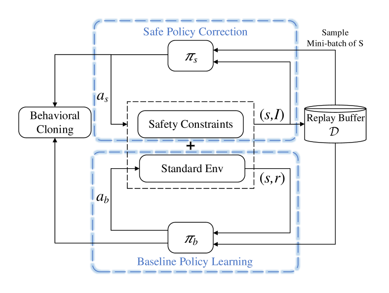
Figure 2: Dual-agent framework for safe robot learning. The baseline policy learning is the standard RL whose objective is the maximization of cumulative rewards. The safe policy correction learns safe behaviors from safety indicator $I$ and imitates the baseline policy via online behavioral cloning.

IV-B Baseline Policy Learning

Baseline policy learning, i.e., problem (10), is a basic RL task that can be solved with a bunch of effective techniques in optimization, exploration and exploitation.

Considering a parametric deterministic policy $\pi_{B}(s;\theta)$, problem (10) is equivalent to:

$$\max_{\theta}\mathop{\mathbb{E}}_{s\sim\mathcal{D}}\big{[}Q_{R}^{\pi_{B}}\big{(}s,\pi_{B}(s;\theta)\big{)}\big{]},$$ (12)

whose parameters can be updated by the deterministic policy gradient (DPG) [25]:

$$\theta\leftarrow\theta+\eta_{\theta}\nabla_{\theta}\pi_{B}(s;\theta)\big{[}\nabla_{a}Q_{R}^{\pi_{B}}(s,a)\big{]}_{a=\pi_{B}(s;\theta)}$$ (13)

IV-C Safe Policy Correction

Safe policy correction, i.e. problem (11), is a constrained optimization problem. Considering a parametric deterministic policy $\pi_{S}(s;\phi)$ and the $L^{2}$-norm distance, problem (11) can be reformulated as:

$$\min_{\phi} \mathop{\mathbb{E}}_{s\sim\mathcal{D}}||\pi_{S}(s;\phi)-\pi_{B}(s;\theta)||^{2}_{2}$$ (14)

$$\mathrm{s.t.} \mathop{\mathbb{E}}_{s\sim\mathcal{D}}\big{[}Q_{I}^{\pi_{S}}\big{(}s,\pi_{S}(s;\phi)\big{)}\big{]}\geq\Gamma$$

Similar to the strong Lagrangian duality in [12], the primal problem (14) can be solved through its dual problem:

$$\max_{\lambda\geq 0}\min_{\phi}\bar{D}(\phi)+\lambda(\Gamma-\bar{Q}(\phi)),$$ (15)

where $\bar{D}(\phi)=\mathop{\mathbb{E}}_{s\sim\mathcal{D}}||\pi_{S}(s;\phi)-\pi_{B}(s;\theta)||^{2}_{2}$ and $\bar{Q}(\phi)=\mathop{\mathbb{E}}_{s\sim\mathcal{D}}\big{[}Q_{I}^{\pi_{S}}\big{(}s,\pi_{S}(s;\phi)\big{)}\big{]}$.

Stochastic primal-dual optimization [26] is applied here to update primal and dual variables alternatively:

(17)

Algorithm 1 Dual-agent Risk-aware Policy Learning.

1:  Initialize safe critics $Q_{\xi_{1}},Q_{\xi_{2}}$ and the risk-aware policy $\pi_{\phi}$.

2:  Initialize target networks ${\xi^{\prime}_{1}}\leftarrow{\xi_{1}},{\xi^{\prime}_{2}}\leftarrow{\xi_{2}},{\phi^{\prime}}\leftarrow{\phi}$.

3:  Initialize the replay buffer $\mathcal{D}$, $\lambda=0$ and $\Gamma$ as in (6).

4:  if the baseline policy $\pi_{\theta}$ is learnable then

5:     Initialize critic $Q_{\omega_{1}},Q_{\omega_{2}}$ and the baseline policy $\pi_{\theta}$.

6:     Initialize target networks ${\omega^{\prime}_{1}}\leftarrow{\omega_{1}},{\omega^{\prime}_{2}}\leftarrow{\omega_{2}},{\theta^{\prime}}\leftarrow{\theta}$.

7:  else

8:     Load the fixed baseline policy $\pi_{\theta}$.

9:  end if

10:  for $t=1$ to $T$ do

11:     if $\upsilon\sim\mathcal{U}(0,1)<0.5$ then

12:        Select action $a\sim\pi_{\theta}(s)+\epsilon,\ \ \epsilon\sim\mathcal{N}(0,\sigma)$.

13:     else

14:        Select action $a\sim\pi_{\phi}(s)+\epsilon,\ \ \epsilon\sim\mathcal{N}(0,\sigma)$.

15:     end if

16:     Calculate safe indicator $I$ as in (2).

17:     Store transition $(s,a,r,I,s^{\prime})$ in the replay buffer $\mathcal{D}$.

18:     Sample mini-batch of N transitions from $\mathcal{D}$.

19:     $//$ Baseline Policy Learning;

20:     if the baseline policy $\pi_{\theta}$ is learnable then

21:        $y\leftarrow r+\gamma\min_{i=1,2}Q_{\omega^{\prime}_{i}}(s^{\prime},\pi_{\theta^{\prime}}(s^{\prime}))$.

22:        Update $\omega_{i}\leftarrow\arg\min_{\omega_{i}}N^{-1}\sum(y-Q_{\omega_{i}}(s,a))^{2}$.

23:        Update $\theta$ as in (13).

24:        Update target networks with Polyak Averaging.

25:     end if

26:     $//$ Safe Policy Correction;

27:     $\bar{y}\leftarrow I+\bar{\gamma}\min_{i=1,2}Q_{\xi^{\prime}_{i}}(s^{\prime},\pi_{\phi^{\prime}}(s^{\prime}))$.

28:     Update $\xi_{i}\leftarrow\arg\min_{\xi_{i}}N^{-1}\sum(\bar{y}-Q_{\xi_{i}}(s,a))^{2}$.

29:     Calculate $\bar{D}(\phi)=\mathop{\mathbb{E}}_{s\sim\mathcal{D}}||\pi_{S}(s;\phi)-\pi_{B}(s;\theta)||^{2}_{2}$.

30:     Update $\phi$ as in (LABEL:phi).

31:     Evaluate $\bar{Q}(\phi)=\mathop{\mathbb{E}}_{s\sim\mathcal{D}}\big{[}Q_{I}^{\pi_{S}}\big{(}s,\pi_{S}(s;\phi)\big{)}\big{]}$.

32:     Update $\lambda$ as in (17).

33:     Update target networks with Polyak Averaging.

34:  end for

Technically, the timescales of primal variable updates are required to be faster than those of Lagrange multipliers (i.e., $\eta_{\phi}\gg\eta_{\lambda}$) [27] to replace the computationally prohibitive minimization of primal variables by a single gradient descent step (LABEL:phi).

IV-D Further Discussion and Detailed Algorithm

We provide further discussions on several useful tricks and insights for better policy improvement in practice. The detailed algorithm is summarized in Algorithm 34.

IV-D1 Initialization

Primal-dual optimization is sensitive to the initialization and learning rate of Lagrange multipliers. In our implementation, we set $\lambda=0$ at the beginning and let $\eta_{\lambda}=0.001$, which enables the agent to learn skills from the baseline policy rapidly and correct dangerous behaviors progressively through interactions.

IV-D2 Exploration

The decoupled framework enables each agent to have an independent reinforcement learning objective, which facilitates the exploration naturally. We suggest selecting actions randomly and alternatively from the two policies, thus each is likely to see more novel and valuable state-action pairs. Moreover, other exploration strategies can be applied directly to the baseline policy learning as in [28].

IV-D3 Over-estimation

The over-estimation due to off-policy Q-learning is catastrophic to $Q^{\pi_{S}}_{I}$ evaluation. To address this issue, the same technique of double Q-learning in [29] is applied, and we suggest a small $\bar{\gamma}$ which is myopic for future safety.

IV-D4 Optimality

Decoupling baseline policy learning and safe policy correction isn’t strictly equivalent to the safe RL problem (8). Thus, our approach only finds a near-optimal policy compared to the primal formulation. Nevertheless, the desirable performance with high sample efficiency usually outweighs the theoretical optimality for most safe robot learning tasks.

$\pi_{b}:t=0$

(a) *

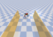
$\pi_{b}:t=100$

(b) *

$\pi_{b}:t=200$

(c) *

$\pi_{b}:t=300$

(d) *

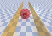
$\pi_{b}:t=400$

(e) *

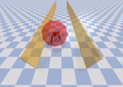
$\pi_{b}:t=500$

(f) *

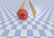
$\pi_{s}:t=0$

(g) *

$\pi_{s}:t=100$

(h) *

$\pi_{s}:t=200$

(i) *

$\pi_{s}:t=300$

(j) *

$\pi_{s}:t=400$

(k) *

$\pi_{s}:t=500$

(l) *

Figure 3: Quadruped robot locomotion task. The agent is rewarded for running through an avenue [30], but violates the safety requirement (marked with a red ball) if it oversteps the non-physical boundaries or exceed the velocity threshold. Rollouts of the baseline policy $\pi_{B}$ and the safe policy $\pi_{S}$ are shown on the top line and bottom line, respectively.

&

$\pi_{b}:t=0$

(a) *

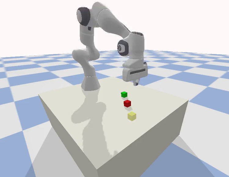
$\pi_{b}:t=10$

(b) *

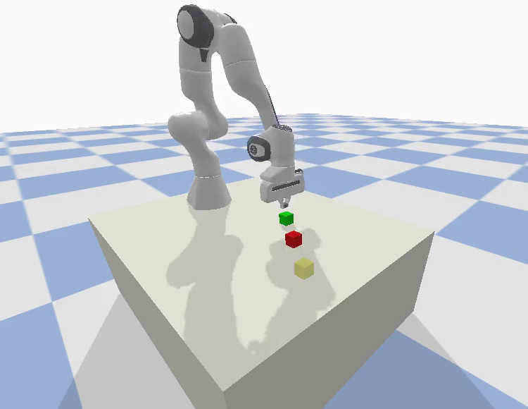
$\pi_{b}:t=20$

(c) *

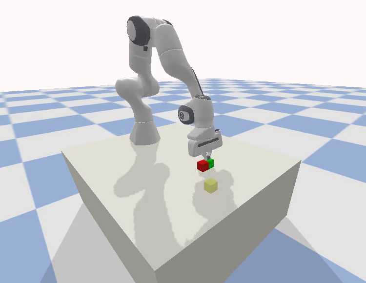
$\pi_{b}:t=30$

(d) *

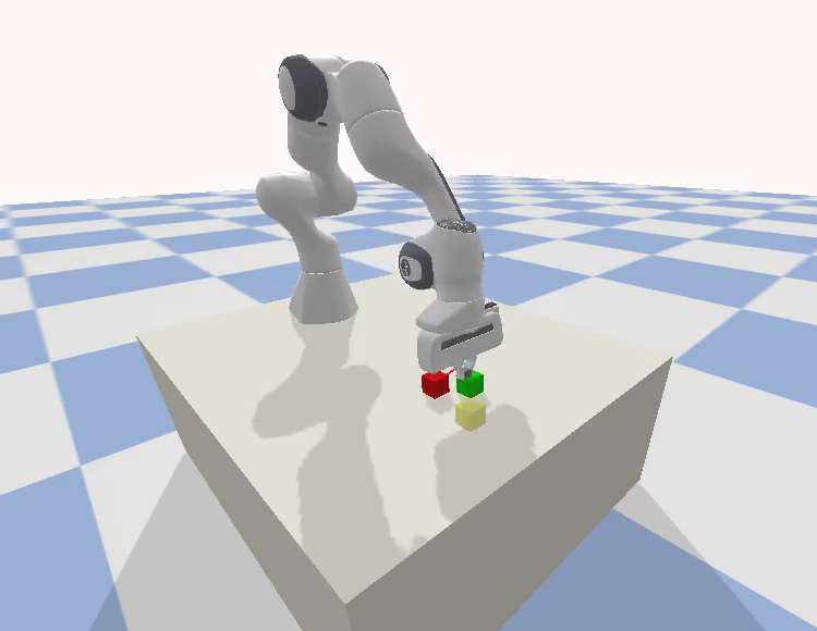
$\pi_{b}:t=40$

(e) *

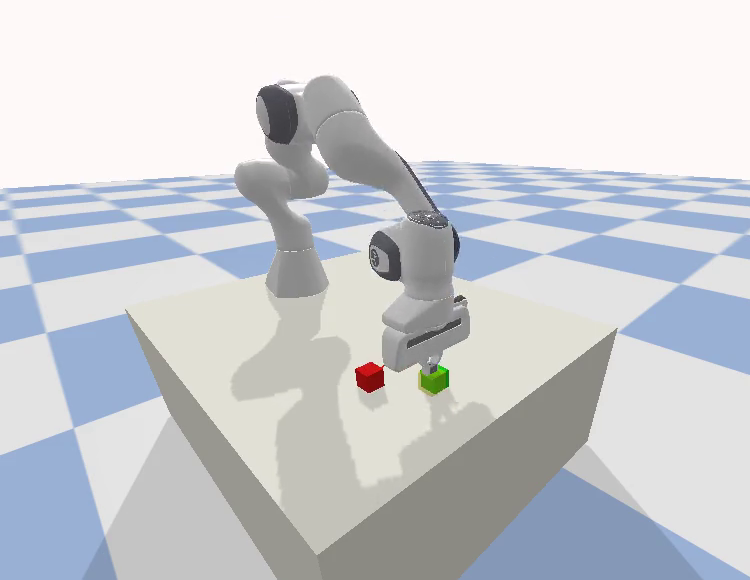
$\pi_{b}:t=50$

(f) *

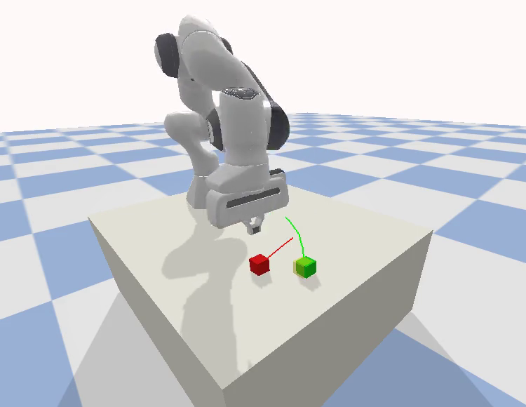
$\pi_{s}:t=0$

(g) *

$\pi_{s}:t=10$

(h) *

$\pi_{s}:t=20$

(i) *

$\pi_{s}:t=30$

(j) *

$\pi_{s}:t=40$

(k) *

$\pi_{s}:t=50$

(l) *

Figure 4: Robotic arm manipulation task. The agent is rewarded for moving the green cube to the destination in yellow, but violates the safety requirement if it collides with the movable red cube. Rollouts of the baseline policy $\pi_{B}$ and the safe policy $\pi_{S}$ are shown on the top line and bottom line, respectively.

&

V EXPERIMENTS

In the experiments, we answer the following questions:

1. Can the baseline agent and the target safe agent learn from scratch synchronously and achieve their goals respectively?

2. Can we correct the safe policy from a pre-trained unsafe model with significantly fewer interactions?

3. Compare to the state-of-art Safe RL algorithms, how much sample efficiency our algorithm improves, and how much difference there is in the final performance?

4. Can our decoupled algorithm leverage pre-trained models and succeed for difficult tasks where previous methods barely learn feasible skills without prior knowledge?

V-A Experimental Setup

We demonstrate the proposed algorithm via two challenging safe robot learning tasks, i.e., the quadruped robot locomotion task and the robotic arm manipulation task. In particular, we train the baseline policy and safe policy synchronously from scratch in the quadruped robot locomotion task, whereas we utilize a fixed pre-trained baseline policy in the robotic arm manipulation task.

The baseline policy (if learnable) and the target safe policy are deterministic with $(400,300)$ hidden layers and activated with $\tanh$ function to restrict the output within action limits.

We compare our algorithm to the state-of-the-art safe RL algorithms, including Constrained Policy Optimization (CPO) [9], Lagrangian relaxation with various RL algorithms (i.e. PPO-L, TRPO-L and SAC-L) [8] and the safety layer correction [13]. To be fair in comparison, we use online supervised learning to initialize agents in the above algorithms if we have already had a baseline controller.

Each experiment is tested over three random seeds.

V-B Environment Details

V-B1 Quadruped Robot Locomotion Environment

As illustrated in Fig. IV-D4, the four-legged ant has to run along the x-direction and is penalized ($I_{t}=1$) for exceeding the velocity limit $1.5m/s$ or crossing the safety boundaries. The observation ($\mathcal{S}\in\mathbb{R}^{33}$) includes the information on the position, velocity and quaternion of each link and joint. The action ($\mathcal{A}\in\mathbb{R}^{8}$) consists of each joint’s torque. $\mathcal{R}$ is calculated by x-velocity. In this experiment, we set time horizon $T=500$ and $\delta=0.05$ (i.e. 0.95-safe policy correction).

V-B2 Robotic Arm Manipulation Environment

The simulated environment is built based on the Panda-gym [31], where the 7-DoF Franka Emika Panda manipulator is used to implement the push task as in Fig. IV-D4. The agent has to push the objective (denoted by a green box) to a target position (denoted by a yellow shadow), but is penalized ($I_{t}=1$) for colliding with the obstacle (denoted by a red box). We adopt position control to move the manipulator end-effector, i.e., the action ($\mathcal{A}\in\mathbb{R}^{3}$) is the increments on X-Y-Z axis. The observation ($\mathcal{S}\in\mathbb{R}^{21}$) consists of (1) the velocity and position of the end-effector, (2) the velocity, rotation and position of the objective, (3) the obstacle position and target position. The environment returns a sparse reward (0 for finished and -1 for unfinished). The time horizon is set as $T=50$, and the positions of the objective and target will be randomly initialized at each round. The obstacle will be placed in the way to target.

V-C Results on Safe Locomotion Task

In this task, the baseline agent and the safe agent are trained synchronously from scratch. Fig. 5 shows the learning processes of the baseline policy $\pi_{B}$ and the target safe policy $\pi_{S}$. At the beginning stage, $\lambda$ is close to zero. Thus $\pi_{S}$ imitates unconstrained $\pi_{B}$, and improves its performance at almost the same speed. The safe agent estimates the future cost and becomes risk-aware via past experiences. As $\lambda$ increases, the penalty for unsafe behaviors dominates the objective function and the return curve of $\pi_{S}$ in Fig. 5(a) falls behind $\pi_{B}$ gradually. Meanwhile, the cost curve of $\pi_{S}$ in Fig. 5(b) drops quickly and satisfies the 0.95-safe requirement at convergence. By contrast, the average episode cost of baseline policy $\pi_{B}$ is close to the episode horizon $500$, which means it violates the safety constraint at almost every step.

As we discussed in Section IV, the decoupled formulation often converges to a reasonable and near-optimal policy at a fast speed. In Table I, we report the performance of our method and other Safe RL methods that solve problem (8) directly. We find our approach has much better sample efficiency than baseline algorithms. After $1\times 10^{6}$ interactions which are relatively expensive in the real-world problem, our method has already converged to a desirable safe policy, whereas other methods still struggle for reward improvement. Generally, previous Safe RL algorithms need 10 to 20 times experience samples than ours for convergence.

It should be noted that the formulation of safe policy correction won’t guarantee a theoretically optimal solution, thus in this task traditional Safe RL algorithms that directly solve (8) would achieve sightly better performance at convergence. Nevertheless, the poor data efficiency makes them impractical in use.

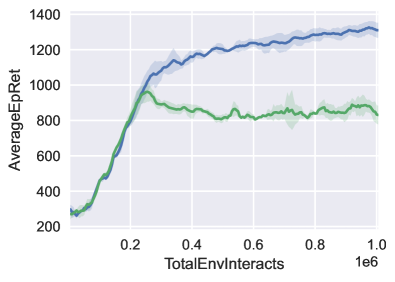
(a) Average Episode Return

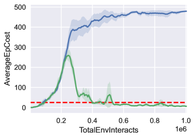
(b) Average Episode Cost

Figure 5: Learning curves of the baseline policy $\pi_{B}$ and the safe policy $\pi_{S}$ on the safe locomotion task. The two agents are trained synchronously in loop. The x-axis is the number of interactions with the emulator. The solid line is the mean and the shaded area is the standard deviation. The dashed line is the expected threshold for 0.95-safe policy.

	Ours	CPO	PPO-L	TRPO-L	SAC-L
Return	898.20	550.43	571.23	546.45	329.87
(1E6 steps)	$\pm 12.29$	$\pm 8.86$	$\pm 11.03$	$\pm 12.55$	$\pm 27.65$
Cost	1.77	3.63	3.33	3.49	2.88
(1E6 steps)	$\pm 0.22$	$\pm 0.86$	$\pm 0.83$	$\pm 0.54$	$\pm 0.26$
Return	898.20	915.36	944.27	917.63	450.24
(Convergence)	$\pm 12.29$	$\pm 10.23$	$\pm 12.77$	$\pm 11.27$	$\pm 22.59$
Cost	1.77	2.65	2.71	2.15	2.12
(Convergence)	$\pm 0.22$	$\pm 0.49$	$\pm 0.51$	$\pm 0.57$	$\pm 0.20$
Total samples	5E5	1E7	1E7	1E7	6E6
	1x	20x	20x	20x	12x

TABLE I: We report average episode return (cumulative rewards) and cost (safety violations) on the safe locomotion task after $10^{6}$ interactions and at convergence. We also show the sample multiples required by baseline algorithms compared to our method.

V-D Results on Safe Manipulation Task

In this task, the baseline agent is pre-trained with Hindsight Experience Replay (HER) [10]. This method is proved to be effective for standard robotic arm manipulation but hasn’t been introduced into Safe RL yet. Thus, it is an actual example explaining how we can directly leverage well-studied techniques in standard RL to our decoupled safe robot learning framework.

Fig. 6 shows the learning processes of the safe policy $\pi_{S}$. At the very beginning, the agent learns some helpful but unsafe behaviors from the fixed baseline. Nevertheless, the off-policy safe RL tuning prohibits it from acting the same as the baseline but modifies its outputs to reduce safety violations under the expected threshold, as illustrated in Fig. 6(b). Also, moving the cube on a curved trajectory degrades the maximum of episode return.

We also plot the evaluation curves of success rate for different algorithms on this task in Fig. 7. Notably, the cube-push task is too difficult to learn for any previous Safe RL algorithm, and none of them can successfully finish the job even once time. Here, we only take CPO as a representative in the plot. In contrast, our approach corrects the safe policy from the pre-trained agent, which requires a small number of interactions and has a high success rate at around 80% finally. To leverage the pre-trained model and be fair in comparison, we also perform the behavior cloning to initialize the agent in Safety Layer and CPO algorithms. This helps them obtain basic skills, but it is still hard to entirely avoid the risk. The success rate stays below 30% after the same number of interactions as our method. We also incorporate a safety layer into the pre-trained model via offline data. The first-order Taylor’s approximation on risk-estimation and overly short-sighted safe action correction limit its success rate at around 50%. Conclusively, our approach has the best the trade-off for desirable performance and sample efficiency.

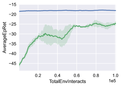
(a) Average Episode Return

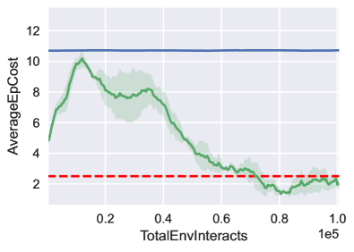
(b) Average Episode Cost

Figure 6: Learning curves of the safe policy $\pi_{S}$ on the safe manipulation task. The pre-trained baseline policy $\pi_{B}$ is fixed during the process. The x-axis is the number of interactions with the emulator. The solid line is the mean and the shaded area is the standard deviation. The dashed line is the expected threshold for 0.95-safe policy.

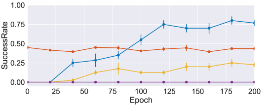
Figure 7: Success rate of different algorithms on the safe manipulation task. A success round counts if the target object is pushed to the destination without the obstacle touched. 20 rounds are evaluated and averaged every 25 epoch (500 steps for each epoch).

VI CONCLUSIONS

In this paper, we propose a dual-agent risk-aware policy learning algorithm for safe policy in robotics. The main idea is to decouple the task into the baseline policy learning and the safe policy correction. The baseline agent can leverage useful techniques in standard RL and even non-learning-based controllers in typical robotic applications; The safe agent is corrected from the baseline with limited data via online behavioral cloning and off-policy constrained RL tuning. Compared to previous Safe RL algorithms, our approach is more data efficient for sample-expensive robotic tasks and achieves more extensive exploration for mastering hard-to-learn skills. Experimental results demonstrate that the proposed method is effective on different, challenging safe robot learning tasks and can obtain a safe and reasonable solution much faster than prior work.

References

- [1] Anthony Francis, Aleksandra Faust, Hao-Tien Lewis Chiang, Jasmine Hsu, J Chase Kew, Marek Fiser, and Tsang-Wei Edward Lee. Long-range indoor navigation with prm-rl. IEEE Transactions on Robotics, 36(4):1115–1134, 2020.
- [2] Aravind Rajeswaran, Vikash Kumar, Abhishek Gupta, Giulia Vezzani, John Schulman, Emanuel Todorov, and Sergey Levine. Learning complex dexterous manipulation with deep reinforcement learning and demonstrations. arXiv preprint arXiv:1709.10087, 2017.
- [3] Sang-Yun Shin, Yong-Won Kang, and Yong-Guk Kim. Obstacle avoidance drone by deep reinforcement learning and its racing with human pilot. Applied sciences, 9(24):5571, 2019.
- [4] Dario Amodei, Chris Olah, Jacob Steinhardt, Paul Christiano, John Schulman, and Dan Mané. Concrete problems in ai safety. arXiv preprint arXiv:1606.06565, 2016.
- [5] Lukas Hewing, Kim P Wabersich, Marcel Menner, and Melanie N Zeilinger. Learning-based model predictive control: Toward safe learning in control. Annual Review of Control, Robotics, and Autonomous Systems, 3:269–296, 2020.
- [6] Yanan Sui, Alkis Gotovos, Joel Burdick, and Andreas Krause. Safe exploration for optimization with gaussian processes. In International conference on machine learning, pages 997–1005. PMLR, 2015.
- [7] Lukas Brunke, Melissa Greeff, Adam W Hall, Zhaocong Yuan, Siqi Zhou, Jacopo Panerati, and Angela P Schoellig. Safe learning in robotics: From learning-based control to safe reinforcement learning. Annual Review of Control, Robotics, and Autonomous Systems, 5, 2021.
- [8] Alex Ray, Joshua Achiam, and Dario Amodei. Benchmarking safe exploration in deep reinforcement learning. arXiv preprint arXiv:1910.01708, 7, 2019.
- [9] Joshua Achiam, David Held, Aviv Tamar, and Pieter Abbeel. Constrained policy optimization. In Doina Precup and Yee Whye Teh, editors, Proceedings of the 34th International Conference on Machine Learning, ICML 2017, Sydney, NSW, Australia, 6-11 August 2017, volume 70 of Proceedings of Machine Learning Research, pages 22–31. PMLR, 2017.
- [10] Marcin Andrychowicz, Filip Wolski, Alex Ray, Jonas Schneider, Rachel Fong, Peter Welinder, Bob McGrew, Josh Tobin, OpenAI Pieter Abbeel, and Wojciech Zaremba. Hindsight experience replay. Advances in neural information processing systems, 30, 2017.
- [11] Yongshuai Liu, Avishai Halev, and Xin Liu. Policy learning with constraints in model-free reinforcement learning: A survey. In Zhi-Hua Zhou, editor, Proceedings of the Thirtieth International Joint Conference on Artificial Intelligence, IJCAI 2021, Virtual Event / Montreal, Canada, 19-27 August 2021, pages 4508–4515. ijcai.org, 2021.
- [12] Santiago Paternain, Miguel Calvo-Fullana, Luiz F. O. Chamon, and Alejandro Ribeiro. Learning safe policies via primal-dual methods. In 2019 IEEE 58th Conference on Decision and Control (CDC), pages 6491–6497, 2019.
- [13] Gal Dalal, Krishnamurthy Dvijotham, Matej Vecerík, Todd Hester, Cosmin Paduraru, and Yuval Tassa. Safe exploration in continuous action spaces. CoRR, abs/1801.08757, 2018.
- [14] Tom Hirshberg, Sai Vemprala, and Ashish Kapoor. Safety considerations in deep control policies with safety barrier certificates under uncertainty. In IEEE/RSJ International Conference on Intelligent Robots and Systems, IROS 2020, Las Vegas, NV, USA, October 24, 2020 - January 24, 2021, pages 6245–6251. IEEE, 2020.
- [15] Todd Hester, Matej Vecerík, Olivier Pietquin, Marc Lanctot, Tom Schaul, Bilal Piot, Dan Horgan, John Quan, Andrew Sendonaris, Ian Osband, Gabriel Dulac-Arnold, John P. Agapiou, Joel Z. Leibo, and Audrunas Gruslys. Deep q-learning from demonstrations. In Sheila A. McIlraith and Kilian Q. Weinberger, editors, Proceedings of the Thirty-Second AAAI Conference on Artificial Intelligence, (AAAI-18), the 30th innovative Applications of Artificial Intelligence (IAAI-18), and the 8th AAAI Symposium on Educational Advances in Artificial Intelligence (EAAI-18), New Orleans, Louisiana, USA, February 2-7, 2018, pages 3223–3230. AAAI Press, 2018.
- [16] Matej Vecerík, Todd Hester, Jonathan Scholz, Fumin Wang, Olivier Pietquin, Bilal Piot, Nicolas Heess, Thomas Rothörl, Thomas Lampe, and Martin A. Riedmiller. Leveraging demonstrations for deep reinforcement learning on robotics problems with sparse rewards. CoRR, abs/1707.08817, 2017.
- [17] Bingyi Kang, Zequn Jie, and Jiashi Feng. Policy optimization with demonstrations. In Jennifer G. Dy and Andreas Krause, editors, Proceedings of the 35th International Conference on Machine Learning, ICML 2018, Stockholmsmässan, Stockholm, Sweden, July 10-15, 2018, volume 80 of Proceedings of Machine Learning Research, pages 2474–2483. PMLR, 2018.
- [18] Mingxuan Jing, Xiaojian Ma, Wenbing Huang, Fuchun Sun, Chao Yang, Bin Fang, and Huaping Liu. Reinforcement learning from imperfect demonstrations under soft expert guidance. In The Thirty-Fourth AAAI Conference on Artificial Intelligence, AAAI 2020, The Thirty-Second Innovative Applications of Artificial Intelligence Conference, IAAI 2020, The Tenth AAAI Symposium on Educational Advances in Artificial Intelligence, EAAI 2020, New York, NY, USA, February 7-12, 2020, pages 5109–5116. AAAI Press, 2020.
- [19] Yang Gao, Huazhe Xu, Ji Lin, Fisher Yu, Sergey Levine, and Trevor Darrell. Reinforcement learning from imperfect demonstrations. In 6th International Conference on Learning Representations, ICLR 2018, Vancouver, BC, Canada, April 30 - May 3, 2018, Workshop Track Proceedings. OpenReview.net, 2018.
- [20] Vinicius G. Goecks, Gregory M. Gremillion, Vernon J. Lawhern, John Valasek, and Nicholas R. Waytowich. Integrating behavior cloning and reinforcement learning for improved performance in dense and sparse reward environments. In Amal El Fallah Seghrouchni, Gita Sukthankar, Bo An, and Neil Yorke-Smith, editors, Proceedings of the 19th International Conference on Autonomous Agents and Multiagent Systems, AAMAS ’20, Auckland, New Zealand, May 9-13, 2020, pages 465–473. International Foundation for Autonomous Agents and Multiagent Systems, 2020.
- [21] Zhaorong Wang, Meng Wang, Jingqi Zhang, Yingfeng Chen, and Chongjie Zhang. Reward-constrained behavior cloning. In Zhi-Hua Zhou, editor, Proceedings of the Thirtieth International Joint Conference on Artificial Intelligence, IJCAI 2021, Virtual Event / Montreal, Canada, 19-27 August 2021, pages 3169–3175. ijcai.org, 2021.
- [22] Lukas Schäfer, Filippos Christianos, Josiah Hanna, and Stefano V Albrecht. Decoupling exploration and exploitation in reinforcement learning. arXiv preprint arXiv:2107.08966, 2021.
- [23] William F Whitney, Michael Bloesch, Jost Tobias Springenberg, Abbas Abdolmaleki, Kyunghyun Cho, and Martin Riedmiller. Decoupled exploration and exploitation policies for sample-efficient reinforcement learning. arXiv preprint arXiv:2101.09458, 2021.
- [24] Eitan Altman. Constrained Markov decision processes, volume 7. CRC Press, 1999.
- [25] David Silver, Guy Lever, Nicolas Heess, Thomas Degris, Daan Wierstra, and Martin Riedmiller. Deterministic policy gradient algorithms. In International conference on machine learning, pages 387–395. PMLR, 2014.
- [26] David G Luenberger, Yinyu Ye, et al. Linear and nonlinear programming, volume 2. Springer, 1984.
- [27] Chen Tessler, Daniel J Mankowitz, and Shie Mannor. Reward constrained policy optimization. In International Conference on Learning Representations, 2018.
- [28] Tianpei Yang, Hongyao Tang, Chenjia Bai, Jinyi Liu, Jianye Hao, Zhaopeng Meng, and Peng Liu. Exploration in deep reinforcement learning: a comprehensive survey. arXiv preprint arXiv:2109.06668, 2021.
- [29] Scott Fujimoto, Herke Hoof, and David Meger. Addressing function approximation error in actor-critic methods. In International conference on machine learning, pages 1587–1596. PMLR, 2018.
- [30] Yinlam Chow, Ofir Nachum, Aleksandra Faust, Edgar Duenez-Guzman, and Mohammad Ghavamzadeh. Lyapunov-based safe policy optimization for continuous control. arXiv preprint arXiv:1901.10031, 2019.
- [31] Quentin Gallouédec, Nicolas Cazin, Emmanuel Dellandréa, and Liming Chen. Multi-goal reinforcement learning environments for simulated franka emika panda robot. CoRR, abs/2106.13687, 2021.